the multi-item capacitated lot-sizing problem with … · abstract — this paper proposes a new...

Abstract— This paper proposes a new mixed integer

programming model for multi-item capacitated lot-sizing problem

with setup times, safety stock and demand shortages in closed-loop

supply chain the returned products from customers can either be

disposed or be remanufactured to be sold as new ones again. The

problem is NP-hard and to solve it, a simulated annulling approach is

used. To verify and validate the efficiency of the SA algorithm, the

results are compared with those of the Lingo 8 software. Results

suggest that the SA algorithm have good ability of solving the

problem, especially in the case of large and medium-sized problems

for which Lingo 8 cannot produce solutions.

Keywords— Closed-loop supply chain, Lot-sizing, Safety stocks,

Simulated annealing.

I. INTRODUCTION

HE production planning problems encountered in real-

life situations are generally intractable due to a number of

practical constraints. The decision maker has to find a good

feasible solution in a reasonable execution time rather than an

optimal one. Their main idea was to find relationships

between the performance of the heuristic and the

computational burden involved in finding the solution. Chen

and Thizy proved that the multi-item capacitated lot-sizing

problem with setup times is strongly NP-hard. There are many

references dealing with the capacitated lot-sizing problem and

to explain why one of the most popular among exact and

approximate solution methods used lagrangian relaxation of

the capacity constraint and compare this approach with every

alternate relaxation of the classical formulation of the

problem[1]. Absi and Kedad-Sidhoum addressed a multi-item

capacitated lot-sizing problem with setup times, safety stock

and demand shortages. They proposed a Lagrangian

relaxation of the resource capacity constraints and developed a

dynamic programming algorithm to solve the problem [2].

Süral et al. considered a lot-sizing problem with setup times

where the objective is to minimize the total inventory carrying

cost only. They proposed some efficient Lagrangian relaxation

Esmaeil. Mehdizadeh, Department of Industrial and Mechanical

Engineering, Qazvin Branch, Islamic Azad University (corresponding author’s

phone: +982813675784; fax: +982813675784; e-mail: [email protected]).

Amir. Fatehi Kivi, Department of Industrial and Mechanical Engineering,

Qazvin Branch, Islamic Azad University (e-mail: [email protected] ).

based heuristics for a lot-sizing problem [3]. Chu et al.

addressed a real-life production planning problem arising in a

manufacturer of luxury goods. This problem can be modeled

as a single-item dynamic lot-sizing model with backlogging,

outsourcing and inventory capacity. They showed that this

problem can be solved in O(T4logT) time where T is the

number of periods in the planning horizon [4]. Golany et al.

studied a production planning problem with remanufacturing.

They proved the problem is NP-complete and obtain an O(T3)

algorithm for solve the problem [5]. Li et al. analyzed a

version of the capacitated dynamic lot-sizing problem with

substitutions and return products. They first applied a genetic

algorithm to determine all periods requiring setups for batch

manufacturing and batch remanufacturing, and then developed

a dynamic programming approach to provide the optimal

solution to determine how many new products are

manufactured or return products are remanufactured in each of

these periods [6]. Pan et al. addressed the capacitated dynamic

lot- sizing problem arising in closed-loop supply chain where

returned products are collected from customers. They assumed

that the capacities of production, disposal and

remanufacturing are limited, and backlogging is not allowed.

Moreover, they proposed a pseudo-polynomial algorithm for

solving the problem with both capacitated disposal and

remanufacturing [7]. Zhang et al. investigated the capacitated

lot-sizing problem in closed-loop supply chain considering

setup costs, product returns, and remanufacturing. They

formulated the problem as a mixed integer program and

propose a Lagrangian relaxation-based solution approach [8].

Tang provides a brief presentation of simulated annealing

techniques and their application in lot-sizing problems [9].

The main contribution of this paper is twofold. First, we

develop the multi-item capacitated lot-sizing problem with

demand shortage, safety stock, deficit costs, capacity stock

and several manners in closed-loop supply chain where

returned products are collected from customers. Then we

design simulated annealing (SA) algorithm to solve the

problem.

II. MATHEMATICAL FORMULATION

In this section, we present an MIP formulation of the

problem. In order to close the gap between the conditions of

The Multi-Item Capacitated Lot-Sizing

Problem With Safety Stocks In Closed-Loop

Supply Chain

Esmaeil Mehdizadeh, and Amir Fatehi Kivi

T

International Journal of Mining, Metallurgy & Mechanical Engineering (IJMMME) Volume 1, Issue 5 (2013) ISSN 2320-4052; EISSN 2320-4060

336

mailto:[email protected]

mailto:[email protected]

the problem and the real world conditions in this research, the

multi-item lot-size problem has been studied with

considerations of production line equilibrium limitation and

capacity limitation. Not only has there been a consideration of

different production manners for products, but also the model

has been designed in the conditions of having safety stock and

shortage being allowed. Also the factory is responsible for

processing used products returned from customers. Two

options are available for these returned products:

remanufacturing and disposal. Remanufactured products can

be sold as new ones with the same quality commitment

[7].The main goal is to present a mathematical model to

optimize production, inventory, outsourcing, shortage,

remanufactured and disposal quantities as well as determine

the best production manner.

A. Assumptions

Before the formulation is considered, the following

assumptions are made on the problem:

I. The demand is considered deterministic. II. The amount of the returned products is regarded

deterministic over the planning horizon. III. Shortage is backlogged. IV. Shortage and inventory costs must be taken into

consideration at the end. V. Raw material resource with given capacities are

considered. VI. The quantity of inventory and shortage at the

beginning of the planning horizon is zero. VII. The quantity of inventory and shortage at the end

of the planning horizon is zero.

B. Parameters

T: Number of periods, indexed from 1 to T, involved in the

planning horizon

N: Number of products, i = 1, …, N

J: Number of production manner, j = 1,…, J

dit: The demand for product i in the period t

Lit: The quantity of the safety stock of product i in the

period t

rit: The selling price per unit of product i in the period t

Cijt: The production cost of each unit of product i in the

period t through the manner j

Aijt: The setup cost of the production of product i in the

period t through the manner j

:ith The unit holding cost of product i in the period t

:ith Unitary safety stock deficit cost of product i in period

t

:it Unitary shortage cost of product i in period t

Bkt: The capacity of the K source at hand in the period t

αik: The quantity of the K source used by each unit of the

product i

fijk: The quantity of wasted K source for product i produced

through the manner j

:it Unit out-sourcing cost of each unit of product i in the

period t

Mi : A large number

:ik The K source consumption for repair of item i

vi : Space needs for per unit of product i

:t The total available space in period t

Fit: The cost of disposing returned products for each unit of

product i in period t

git: The cost of remanufacturing returned products for each

unit of product i in period t

:it The unit holding cost of product i of returned products

in period t

:d

itC The maximum number of returned products of product

i that could be disposed in period t

:r

itC The maximum number of returned products of product

i that could be remanufactured in period t

Rit: the number of returned products of product i in period t

Decision Variables

Xijt: Production quantity for product i in the period t

through the manner j

:f

itX The number of returned products of product i that

remanufactured in period t

:s

itX The number of returned products of product i that

disposed in period t

yijt: Binary variable; 1 if the product i is produced in the

period t through the manner j, otherwise ijty =0

Uit: Out-sourcing level of product i in the period t

:r

itI The number of returned products of product i held that

in inventory at the end of period t

:itI The quantity of shortage of product i in the period t

:itS The quantity of overstock deficit of product i in the

period t

:itS The quantity of safety stock deficit of product i in the

period t

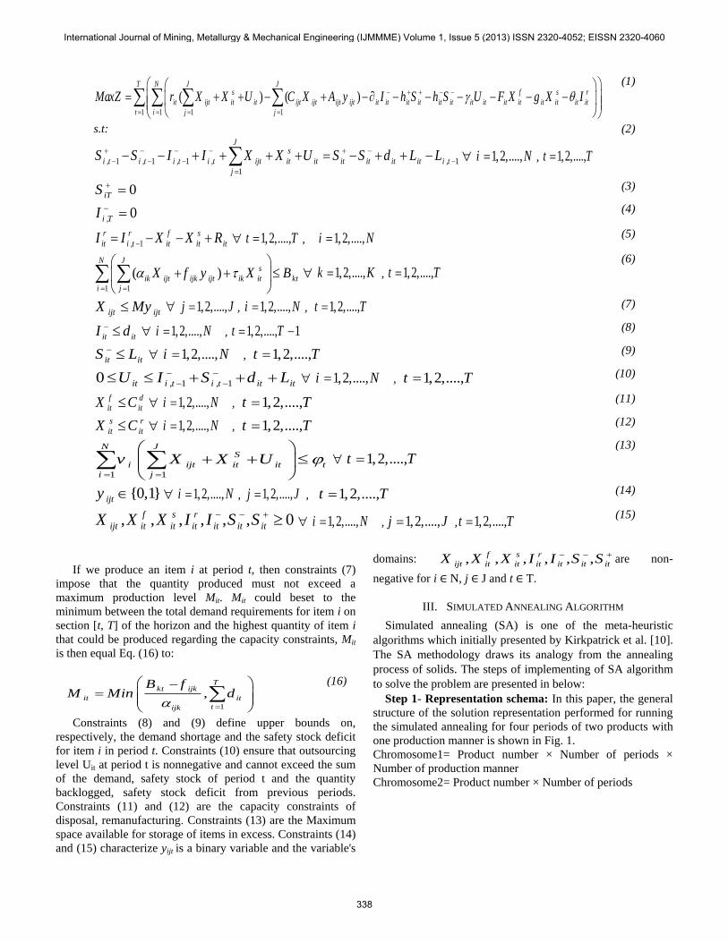
The objective function (1) shows difference between selling

price with the total cost. Constraints (2) are the inventory flow

conservation equations through the planning horizon.

Constraints (3) and (4) define respectively, the demand

shortage and the safety stock deficit for item i at end period is

zero. Constraints (5) are the inventory flow conservation

equations for returned products. Constraints (6) are the

capacity constraints; the overall consumption must remain

lower than or equal to the available capacity.


337

1 1 1 1

( ) ( )T N J J

s f s r

it ijt it it ijt ijt ijt ijt it it it it it it it it it it it it it it

t i j j

MaxZ r X X U C X A y I h S h S U F X g X I

(1)

s.t:

, 1 , 1 , 1 , , 1

1

Js

i t i t i t i t ijt it it it it it it i t

j

S S I I X X U S S d L L

1,2,....,i N , 1,2,....,t T

(2)

0iTS (3)

, 0i TI (4)

, 1

r r f s

it i t it it itI I X X R 1,2,....,t T , 1,2,....,i N (5)

1 1

( )N J

s

ik ijt ijk ijt ik it kt

i j

X f y X B

1,2,....,k K , 1,2,....,t T

(6)

ijt ijtX My 1,2,....,j J , 1,2,....,i N , 1,2,....,t T (7)

it itI d 1,2,....,i N , 1,2,...., 1t T (8)

it itS L 1,2,....,i N , 1,2,....,t T (9)

, 1 , 10 it i t i t it itU I S d L

1,2,....,i N , 1,2,....,t T (10)

f d

it itX C 1,2,....,i N , 1,2,....,t T (11)

s r

it itX C 1,2,....,i N , 1,2,....,t T (12)

1 1

N JS

i ijt it it t

i j

v X X U

1,2,....,t T

(13)

{0,1}ijty 1,2,....,i N , 1,2,....,j J , 1,2,....,t T (14)

, , , , , , 0f s r

ijt it it it it it itX X X I I S S 1,2,....,i N , 1,2,....,j J , 1,2,....,t T (15)

If we produce an item i at period t, then constraints (7)

impose that the quantity produced must not exceed a

maximum production level Mit. Mit could beset to the

minimum between the total demand requirements for item i on

section [t, T] of the horizon and the highest quantity of item i

that could be produced regarding the capacity constraints, Mit

is then equal Eq. (16) to:

1

,T

kt ijk

it it

tijk

B fM Min d

(16)

Constraints (8) and (9) define upper bounds on,

respectively, the demand shortage and the safety stock deficit

for item i in period t. Constraints (10) ensure that outsourcing

level Uit at period t is nonnegative and cannot exceed the sum

of the demand, safety stock of period t and the quantity

backlogged, safety stock deficit from previous periods.

Constraints (11) and (12) are the capacity constraints of

disposal, remanufacturing. Constraints (13) are the Maximum

space available for storage of items in excess. Constraints (14)

and (15) characterize yijt is a binary variable and the variable's

domains: , , , , , ,f s r

ijt it it it it it itX X X I I S S are non-

negative for i ∈ N, j ∈ J and t ∈ T.

III. SIMULATED ANNEALING ALGORITHM

Simulated annealing (SA) is one of the meta-heuristic

algorithms which initially presented by Kirkpatrick et al. [10].

The SA methodology draws its analogy from the annealing

process of solids. The steps of implementing of SA algorithm

to solve the problem are presented in below:

Step 1- Representation schema: In this paper, the general

structure of the solution representation performed for running

the simulated annealing for four periods of two products with

one production manner is shown in Fig. 1.

Chromosome1= Product number × Number of periods ×

Number of production manner

Chromosome2= Product number × Number of periods


338

Fig. 1 Solution representation

Step 2- Neighborhood scheme: At each temperature level

a search process is applied to explore the neighborhoods of

the current solution. In this paper we use mutation scheme,

Fig. 2 illustrates this operation on the each of four periods of

two products with one production manner.

Fig. 2 An example of the neighborhood structure

Step 3- Cooling schedule scheme: Initially, T is set to a

high value, Ti, and it can be reduced with some patterns at

each step of algorithm. The cooling schedule with Ti = α × Ti -

1 (where α is the cooling factor constant α ϵ (0, 1) is

considered as cooling pattern for this research.

Step 4- Termination condition: The SA continues the

above procedure until the termination condition is satisfied (T

< TF). Initial and final temperatures have pre-determined

constant set.

Remark: because in this model objective function is type of

maximum, we have to multiply our objective function in the

negative.

IV. EXPERIMENTAL RESULTS

We try to test the performance of the SA in finding good

quality solutions in reasonable time for the problem. For this

purpose, 15 problems with different sizes are generated. These

test problems are classified into three classes: small size,

medium size and large size multi-item capacitated lot-sizing

problem with safety stocks in closed-loop supply chain

problems. The number of products, production manners and

periods has the most impact on problem hardness. The

proposed model coded with Lingo (ver.8) software using for

solving the instances and the SA is implemented to solve each

instance in five times to obtain more reliable data. For

implementation SA algorithm, the parameters set as: T0 =

1000, α=0.99, L=50 and Tf =0. The best results are recorded

as a measure for the related problem. Table 1 shows details of

computational Selection: Highlight all author and affiliation

lines.

TABLE I.

DETAILS OF COMPUTATIONAL RESULTS FOR ALL TEST PROBLEMS

Objective Function Value (OFV)

No Class

Product

manner Period

Lingo SA

OFV Time OFV Time

1 Small 2 2 3 1366842 0 1366842 6

2 2 2 5 2170470 0 2165482 26

3 2 3 5 2180288 1 2165482 31

4 5 3 5 4692306 100 4286763 62

5 5 2 6 5497372 300 5037989 75

6 Medium 5 3 6 5621934 750 4997012 341

7 5 4 7 6832705 1011 5950741 369

8 5 3 8 ------- ------- 6754581 388

9 5 4 8 ------- ------- 10134054 400

10 6 3 9 ------- ------- 8551200 680

11 Large 5 3 10 ------- ------- 8624198 700

12 6 3 11 ------- ------- 9571335 735

13 6 4 12 ------- ------- 10601543 760

14 6 3 12 ------- ------- 19109673 850

15 6 4 12 ------- ------- 11650807 900

— Means that a feasible solution has not been found after 3600 s of computing time.


339

[50000,70000], [60,95], [16000,30000], [1,8], [12,18]

[7,11], [12,17], 1 [1,4]

[65,85], [65,85], [

2, 20,

15,20]

1, 1, f 1,

[1,2, [7,9], ], [

it ijt ijt it it

it it kt it

it it

t i ijk ijk

d r

ii it tt ti

r C A d

h h B V

C C

L

F F g

1,3], [1,3]itR

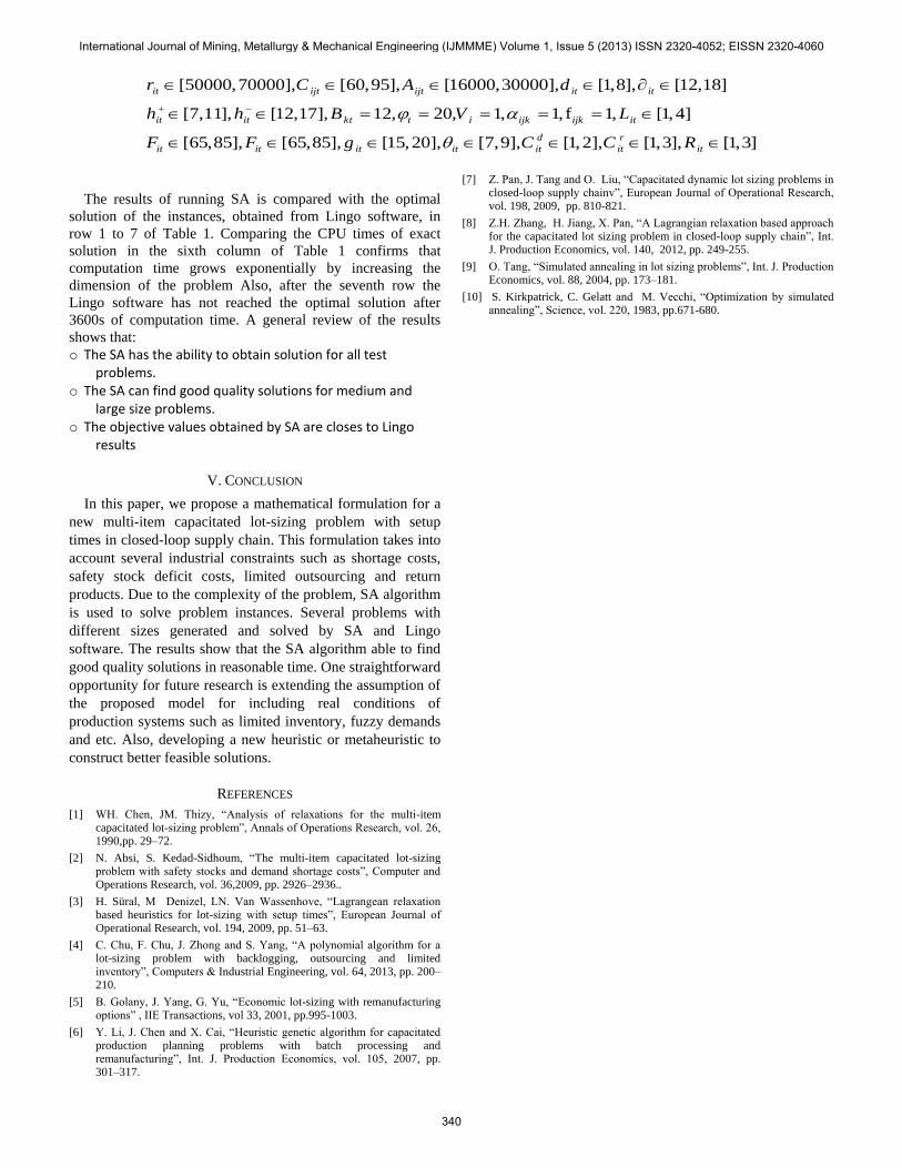
The results of running SA is compared with the optimal

solution of the instances, obtained from Lingo software, in

row 1 to 7 of Table 1. Comparing the CPU times of exact

solution in the sixth column of Table 1 confirms that

computation time grows exponentially by increasing the

dimension of the problem Also, after the seventh row the

Lingo software has not reached the optimal solution after

3600s of computation time. A general review of the results

shows that:

o The SA has the ability to obtain solution for all test problems.

o The SA can find good quality solutions for medium and large size problems.

o The objective values obtained by SA are closes to Lingo results

V. CONCLUSION

In this paper, we propose a mathematical formulation for a

new multi-item capacitated lot-sizing problem with setup

times in closed-loop supply chain. This formulation takes into

account several industrial constraints such as shortage costs,

safety stock deficit costs, limited outsourcing and return

products. Due to the complexity of the problem, SA algorithm

is used to solve problem instances. Several problems with

different sizes generated and solved by SA and Lingo

software. The results show that the SA algorithm able to find

good quality solutions in reasonable time. One straightforward

opportunity for future research is extending the assumption of

the proposed model for including real conditions of

production systems such as limited inventory, fuzzy demands

and etc. Also, developing a new heuristic or metaheuristic to

construct better feasible solutions.

REFERENCES

[1] WH. Chen, JM. Thizy, “Analysis of relaxations for the multi-item capacitated lot-sizing problem”, Annals of Operations Research, vol. 26, 1990,pp. 29–72.

[2] N. Absi, S. Kedad-Sidhoum, “The multi-item capacitated lot-sizing problem with safety stocks and demand shortage costs”, Computer and Operations Research, vol. 36,2009, pp. 2926–2936..

[3] H. Süral, M Denizel, LN. Van Wassenhove, “Lagrangean relaxation based heuristics for lot-sizing with setup times”, European Journal of Operational Research, vol. 194, 2009, pp. 51–63.

[4] C. Chu, F. Chu, J. Zhong and S. Yang, “A polynomial algorithm for a lot-sizing problem with backlogging, outsourcing and limited inventory”, Computers & Industrial Engineering, vol. 64, 2013, pp. 200–210.

[5] B. Golany, J. Yang, G. Yu, “Economic lot-sizing with remanufacturing options” , IIE Transactions, vol 33, 2001, pp.995-1003.

[6] Y. Li, J. Chen and X. Cai, “Heuristic genetic algorithm for capacitated production planning problems with batch processing and remanufacturing”, Int. J. Production Economics, vol. 105, 2007, pp. 301–317.

[7] Z. Pan, J. Tang and O. Liu, “Capacitated dynamic lot sizing problems in closed-loop supply chainv”, European Journal of Operational Research, vol. 198, 2009, pp. 810-821.

[8] Z.H. Zhang, H. Jiang, X. Pan, “A Lagrangian relaxation based approach for the capacitated lot sizing problem in closed-loop supply chain”, Int. J. Production Economics, vol. 140, 2012, pp. 249-255.

[9] O. Tang, “Simulated annealing in lot sizing problems”, Int. J. Production Economics, vol. 88, 2004, pp. 173–181.

[10] S. Kirkpatrick, C. Gelatt and M. Vecchi, “Optimization by simulated annealing”, Science, vol. 220, 1983, pp.671-680.


340

the multi-item capacitated lot-sizing problem with … · abstract — this paper proposes a new...

Documents