1

An HNP-MP Approach for the CapacitatedMulti-item Lot Sizing Problem with Setup Times

Tao Wu, Leyuan Shi, Senior Member, IEEE, and Neil A. Duffie

Abstract—In this paper we consider the capacitated multi-itemlot sizing problem with setup times. The problem is to scheduleJ different items over a horizon of T periods with the objectiveto minimize the sum of setup cost and inventory holding cost. Toachieve feasible high quality solutions, we propose a new solutionapproach which hybrids Nested Partitions and MathematicalProgramming (HNP-MP). Nested Partitions is a partitioning andsampling based heuristic method with a global perspective onthe problem. In the proposed new method the MathematicalProgramming method is implemented to calculate the promisingindex and to provide a good guidance on partitioning in theNested Partitions framework. A time-oriented decompositionheuristic method, Relax-and-Fix, is also implemented to obtaingood promising regions and speed up the computational process.Computational results based on benchmark test problems showthat the approach is computationally tractable and is able toobtain good results. The approach outperforms other state-of-the-art approaches found in the literature.

Note to Practitioners—The capacitated multi-item lot sizingproblem with setup times considered in this paper is motivatedby the attempt of effectively planning the production with lowersetup cost and inventory holding cost under the constraints oflimited capacities. An effective production planning on a lotsizing problem can provide a good guidance on the decisionmade by a Material Requirements Planning (MRP) system, andcheck for the conflicts with available capacities. Two areas ofapproaches are implemented to deal with the problem: the exactapproach and the heuristic approach. The main drawback ofthe exact approach is the excessive computational time whenthe problem size becomes large. On the other hand, the maindrawback of the heuristic approach is an inefficient objectivesolution. The goal of this paper is to propose a heuristic approachwhich outperforms other state-of-the-art approaches found in theliterature. Practitioners can apply the proposed method into theextensions of lot sizing problems which consider backlogging,overtime, and shortage.

Index Terms—Capacitated Multi-item Lot Sizing, Dantzig-Wolfe Decomposition, Nested Partitions, Column Generation,Relax-and-Fix.

I. INTRODUCTION

The paper addresses the capacitated single-level multi-itemlot sizing problem with setup times (CLST). The problemis to plan the production of J items over a horizon of T

Tao Wu is with the Department of Industrial and Systems Engineer-ing, University of Wisconsin-Madison, Madison, WI, 53706 USA (e-mail:twu5@wisc.edu).

Leyuan Shi is with the Department of Industrial and Systems Engineer-ing, University of Wisconsin-Madison, Madison, WI, 53706 USA (e-mail:leyuan@engr.wisc.edu).

Neil A. Duffie is with the Department of Mechanical Engineering,University of Wisconsin-Madison, Madison, WI, 53706 USA (e-mail:duffie@engr.wisc.edu).

Manuscript received Feb. 16, 2009.

periods in which the throughput time is one period. Demandsare specified for each item in each period and should besatisfied without backlogging. However, initial inventory isallowed to avoid the infeasibility of a production plan. Theobjective is to find a minimum cost production plan withoutviolating the capacity constraints in each period. The total costof any production plan contains three components: setup cost,inventory holding cost and initial inventory holding cost. Thefollowing assumptions are addressed in the problem. Setuptimes and cost are non-sequence dependent. There are nolinked lot sizes, e.g. no distinction between major setups forproduct types and minor setups for items. The possibility ofsetup carryover between periods is neglected. The investigatedmodel is of the big-bucket type that does not consider the time-phasing of production activities within a period. In particular,the investigated model does not exclude interferences betweenthe production activities at different machines. The lot sizingproblem reflects the settings of an MRP and control environ-ment based on the push principle. The solution procedures thathave been applied to solve the CLST can be generally dividedinto two areas.

The first area encompasses the exact solution approachesrelated to Mathematical Programming, which itself containstwo groups. The first group strengthens the original formu-lation by adding valid inequalities. Barany et al. [1] proposevalid inequalities that define the polytope of the uncapacitatedsingle-item lot sizing problem. Pochet and Wolsey [2], Wolsey[3], and Miller et al. [4] add strong valid inequalities to theoriginal model formulation to speedup solving these lot sizingproblems. The second group within this method attemptsto create strong reformulations. Two of the most prominentreformulation models are the Facility Location reformulationand the Shortest Path reformulation proposed by Krarup andBilde [5] and Eppen and Martin [6], respectively. Stadtler [7]proposes another reformulation model. However, experienceshows that exact solution approaches cannot handle largemathematical mixed-integer programming problems becauseof unacceptably long solution times; only small probleminstances can be solved within reasonable time limits.

The other area of solution procedures involves heuristicmethods, such as the neighborhood search, item orienteddecomposition, and time-oriented decomposition approaches.Such methods are more often implemented in research papersthan exact solution approaches because even the capacitatedsingle-item lot sizing problem has been shown to be NP-hard by Florian et al. [8]. Belvaux and Wolsey [9] proposea method, which is a specialized Branch-and-Cut and time-oriented decomposition heuristic method for lot sizing prob-

2

lems. Federgruen et al. [10] develop and analyze a classof so-called progressive interval heuristics to the CLST. Inaddition, Degraeve and Jans [11] describe an implementationof a Branch-and-Price algorithm to the CLST. A combinationof simplex optimization and subgradient updating is used tospeed up the Column Generation process.

In other heuristic implementations, Trigeiro et al. [12] andTempelmeier and Derstroff [13] propose Lagrangian baseddecomposition methods for the large scale lot sizing problem.Salomon [14] develops a tabu search procedure where thesolution set is searched quickly in a greedy fashion. Simpsonand Erenguc [15] develop a neighborhood search heuristicmethod. Sahling et al. [16] propose an MIP-based fix-and-optimize approach that solves a series of mixed-integer linearprograms iteratively for the dynamic multi-level capacitated lotsizing problem with setup carry-overs. Absi et al. [17] proposemixed integer programming heuristics based on a planninghorizon decomposition strategy to find a feasible solution forthe multi-item capacitated lot-sizing problem with setup timesand shortage costs. Pochet et al. [18] develop a library oftools for solving production planning problems that is calledas LS-LIB. LS-LIB is embedded into an optimization software,XPRESS, and is very powerful to solve production planningproblems. The strength of the heuristic methods is their abilityto obtain the fairly good feasible solutions or upper boundswithin a reasonable time frame. However, the duality gapbetween the upper bound and lower bound can be unacceptablebecause the upper bounds achieved by the heuristic methodsare insufficient. We therefore propose a new solution approachwhich is called the Hybrid Nested Partitions and MathematicalProgramming approach (HNP-MP).

Nested Partitions is a partitioning and sampling basedmethod that focuses computational effort on the most promis-ing region of the solution space while maintaining a globalperspective on the problem [19]. It has been efficiently appliedto a wide range of Mixed Integer Programming problems suchas the traveling salesman problem [20], the product designproblem [21], and the local pickup and delivery problem [22].In the Nested Partitions framework, calculating the promisingindex of each region is critical to having the fast convergencerate and obtaining good feasible solutions. Nested Partitionscould be implemented to the CLST directly. However, it wouldbe hard to find a good partitioning and sampling strategy if itis just used individually. Here, the lower bounds found usingColumn Generation or Simplex and upper bounds found usinga time-oriented decomposition heuristic method, Relax-and-Fix, are used to define intelligent partitioning that improvesthe efficiency of the Nested Partitions method. The solutions inboth upper bounds and lower bounds are utilized and provideguidance on partitioning and sampling in Nested Partitions.Also, the efficiency of the method could be achieved by settinga comparatively small mount of time to each subproblem forthe Relax-and-Fix algorithm; it then would not consume muchcomputational effort.

The remainder of the paper is organized as follows: AFacility Location model formulation for the CLST is givenin Section II. In Section III, a Dantzig-Wolfe Decompositionreformulation of the Facility Location model is described and

a Column Generation algorithm is proposed to solve its LinearProgramming (LP) relaxation problem. Nested Partitions andRelax-and-Fix are also introduced in this section. After that theHNP-MP approach is proposed. In Section IV, a further ex-tension analysis of HNP-MP is given. Detailed computationaltests based on benchmark problems are given in Section V.Finally, our conclusions and future research are presented inSection VI.

II. THE MODEL FORMULATION FOR THE CLSTSeveral model formulations yielding different model sizes

and lower bounds have been proposed for the CLST in theliterature. We formulate the problem as a Facility Locationproblem, which was originally proposed by Krarup and Bilde[5] for single-item problems. The Facility Location formu-lation is able to provide a strong lower bound when its LPrelaxation problem is solved. In order to present the modelformulation clearly, notations are given as follows:

Indices and Index Sets:

T Number of periods.J Number of items.M Number of machines.t, s Periods, t, s = 1, . . . , T .j Items, j = 1, . . . , J .m Machines, m = 1, . . . , M .

Parameters:

scj Setup cost for a lot of item j.STjm Setup time for item j on machine m.Cmt Available capacity of machine m in period t.hcj Inventory holding cost for one unit of item j in a

period.gcjt Unit cost of initial inventory for item j to be used

in period t.ajm Production time necessary to produce one unit of

item j on machine m.djt Demand for item j in period t.

Variables:

Xjts The amount of item j produced in period t to meetdemand in period s (t ≤ s).

Ijt The amount of initial inventories of item j to meetdemand in period t, these variables are similar to lo-st sales or shortages known in the literature [23] or[17].

Yjt Binary setup variable (=1, if item j is produced inperiod t; 0 otherwise).

The formulation of the problem, which we refer to as theFacility Location (FL) model formulation, can be then statedas follows:

FL:

min

J∑j=1

T∑t=1

scjYjt +

J∑j=1

T∑t=1

T∑s=t

(s− t)hcjXjts

3

+J∑

j=1

T∑t=1

gcjtIjt. (1)

s.t.s∑

t=1

Xjts + Ijs = djs ∀ j = 1, . . . , J, s = 1, . . . , T. (2)

J∑j=1

T∑s=t

ajmXjts +

J∑j=1

STjmYjt ≤ Cmt

∀ m = 1, . . . ,M, t = 1, . . . , T. (3)

Xjts ≤ djsYjt ∀ j = 1, . . . , J, t = 1, . . . , T,

s = t, . . . , T. (4)

Ijt ≥ 0; Xjts ≥ 0; Yjt ∈ {0, 1} ∀ j = 1, . . . , J,

t, s = 1, . . . , T. (5)

The objective function (1) minimizes total setup, inventoryholding, and initial inventory holding costs during the plan-ning horizon. Constraints (2) ensure demand satisfaction inall periods for all items. Constraints (3) enforce capacityrequirements. Constraint set (4) ensures that the total amountof production is less than sufficiently large value and that asetup is performed in period t for item j if any demand issatisfied using the corresponding production. Constraints (5)enforce the binary and nonnegative requirements for differentvariables.

III. THE HNP-MP APPROACH FOR THE CLST

In order to present the HNP-MP approach clearly, we firstlymake a brief introduction to the Nested Partitions method inthis section. A Dantzig-Wolfe Decomposition reformulation ofthe FL model is presented and a Column Generation algorithmis implemented to solve its LP relaxation problem, whichprovides a strong lower bound and a guideline on calculatingthe promising index for HNP-MP. A Relax-and-Fix method isalso implemented, it helps find a good promising region andimproves the computational speed for HNP-MP. Finally, wemake a detailed explanation of the implementation of HNP-MP.

A. Nested Partitions

The Nested Partitions method is a partitioning and samplingbased strategy that focuses computational effort on the mostpromising region of the solution space while maintaining aglobal perspective on the problem. In each iteration of thealgorithm, the entire solution space is viewed as the unionof a promising region and a surrounding region. The actualNested Partitions iteration comprises four steps, which weoutline below:

The first step of each iteration is to partition the current mostpromising region into several subregions and aggregate thesurrounding region into one region. The partitioning strategyimposes a structure on the feasible region and is therefore very

important for the convergence algorithm. If the partitioning issuch that most of the good solutions to the problem tend to beclustered together in subregions, it is likely that the algorithmquickly concentrates the search in these subsets of the feasibleregion. It should be noted that a good partitioning strategyalways exists but may not be easy to identify.

The next step of the algorithm is to randomly sample fromeach of the subregions and from the aggregated surroundingregion. This can be done in almost any fashion. The onlycondition is that each solution in a given sampling regionshould be selected with a positive probability. Clearly, uni-form sampling can always be chosen as the generic option.However, it may often be worthwhile to incorporate a specialstructure into the sampling procedure. The aim of such asampling method should be to select good solutions with ahigher probability than poor solutions

Once each region has been sampled, the next step is touse the sample points to calculate the promising index ofeach region. Again, the Nested Partitions methodology offersa great deal of flexibility. The only requirement imposed on apromising index is that it agrees with the original performancefunction on regions of maximum depth, i.e., on singletonsthat are regions containing only a single point. Due to such asimple requirement, many local search heuristics can be usedin this step to construct a promising index [19].

If one of the subregions has the best promising index, thealgorithm moves to this region and considers it to be themost promising region in the next iteration. If the surroundingregion has the best promising index, the algorithm backtracks.This can be done in several manners; two of which will bediscussed here. The first alternative considered is backtrackingall the way to the top, i.e., to the entire feasible region.The second is to backtrack to the superregion of the currentmost promising region. Both of these backtracking rulesensure asymptotic convergence. [19] can be referred for moreinformation on Nested Partitions.

B. The Dantzig-Wolfe Decomposition and Column GenerationApproach for the CLST

The Dantzig-Wolfe Decomposition approach is an applica-tion of using a pricing mechanism that has been developedfor a wide class of mathematical programs, especially forthose problems with complicating or linking constraints. Itchooses to solve a large number of smaller size, typicallywell-structured, subproblems instead of solving the originalproblem whose size and complexity are beyond what canbe solved within a reasonable amount of time. Also, thelower bound provided by the relaxation problem of Dantzig-Wolfe Decomposition is stronger than that obtained fromthe relaxation of the original problem. For the CLST, theoriginal problem is here separated into a master problem andJ subproblems in the Dantzig-Wolfe Decomposition method.All generated columns in the master problem are the vertexpoints of the convex space defined by the constraints in Jsubproblems. The master problem has capacity constraints andconvexity constraints for all columns. While J subproblemsare independent uncapacitated single item lot sizing problems.

4

The Dantzig-Wolfe Decomposition approach for the CLSTis addressed by a number of authors including Vanderbecket al. [24] and Degraeve and Jans [11]. Most of them dealwith the LP relaxation of the master problem in order toobtain a lower bound. In this paper we implement the Dantzig-Wolfe Decomposition into the FL model formulation (FL-DD) because it provides a strong lower bound. It is similarto those used by Manne [25] and Degraeve and Jans [11].However, the lower bounds achieved by the Dantzig-WolfeDecomposition used in the paper are better than theirs becausethey implement the Dantzig-Wolfe Decomposition on a weakformulation. Please refer [25] for more details. Let q ∈ Qj

where Qj is defined as the set of all possible setup schedulesfor item j, Qj = (Yj1, . . . , YjT )|Yjt ∈ (0, 1) ∀ t ∈ 1, . . . , T .Y qjt is one if there is a setup for item j in period t in setup

schedule q; zero otherwise. Xqjts is defined as the amount of

item j produced in period t to meet the demand in periods (t ≤ s) in setup schedule q, Iqjt is defined as the amountof initial inventories of item j to meet demand in period t insetup schedule q, and zjq is defined as the fraction of scheduleq for product j that will be produced. The master problemformulation of FL-DD, which is referred to as FLM, is thengiven as follows:

FLM:

min

J∑j=1

T∑t=1

∑q∈Qj

scjYqjtzjq+

J∑j=1

T∑t=1

T∑s=t

∑q∈Qj

(s−t)hcjXqjts·

zjq +J∑

j=1

T∑t=1

∑q∈Qj

gcjIqjtzjq (6)

s.t. ∑q∈Qj

zjq = 1 ∀ j = 1, . . . , J (7)

J∑j=1

∑q∈Qj

T∑s=t

ajmXqjtszjq +

J∑j=1

∑q∈Qj

STjYqjtzjq ≤ Cmt

∀ m = 1, . . . ,M, t = 1, . . . , T (8)

zjq ≥ 0 ∀ j = 1, . . . , J, q ∈ Qj (9)

For the CLST, Column Generation starts with a restrictedmaster problem with only a few columns obtained from the un-capacitated single-item lot sizing pricing problem. Therefore,the initial restricted master problem FLM may be infeasiblebecause the integrality capacity constraints may not be satis-fied. In order to get a feasible initial FLM, we can either use aheuristic method to generate some feasible initial columns inFLM, or slightly modify FLM by adding an artificial variableto the right-hand side of each of the integrality capacityconstraints (8) and considering this artificial variable as theobjective function. The second technique, adding an artificialvariable, is used in this paper, and the problem is referredto as being in Phase1 when the added artificial variable ispositive. Note that the feasible polyhedron for the lot sizingproblem is bounded because the ending inventory must bezero. Otherwise, a linear combination of extreme rays needs

also to be considered. The master problem FLM1 and thepricing subproblem FLS1 in Phase1 are stated as follows. Notethat the artificial variable Of is introduced in Phase1 to avoidinfeasible initial columns. Below we will use πmt (m = 1,. . . , M , t = 1, . . . , T ) as the dual variables associated withthe joint capacity constraints (11), and uj (j = 1, . . . , J) asdual variables for the second set of constraints (12), known asconvexity constraints.

FLM1:

min Of (10)

s.t.J∑

j=1

∑q∈Qj

T∑s=t

ajmXqjtszjq +

J∑j=1

∑q∈Qj

STjmY qjtzjq ≤ Cmt

+Of ∀ t = 1, .., T, m = 1, ..,M (11)

∑q∈Qj

zjq = 1 ∀ j = 1, . . . , J (12)

zjq ≥ 0. ∀ j = 1, . . . , J, q ∈ Qj (13)

FLS1:

maxT∑

t=1

T∑s=t

M∑m=1

ajmπmtXjts +T∑

t=1

M∑m=1

STjmπmtYjt

+uj ∀ j = 1, . . . , J (14)

s.t. (2), (4), (5)

When the optimal solution of Of in FLM1 is non-positiveafter plugging more and more columns into the master problemFLM1. The problem is moved to Phase2, in which the masterproblem FLM2 and the pricing subproblem FLS2 are given asfollows. Note that Of is set as 0 in Phase2.

FLM2:

minJ∑

j=1

∑q∈Qj

T∑t=1

T∑s=t

(s− t)hcjXqjtszjq +

J∑j=1

∑q∈Qj

T∑t=1

scjYqjtzjq +

J∑j=1

∑q∈Qj

T∑t=1

gcjtIqjtzjq (15)

s.t. (11), (12), (13).

FLS2:

max

T∑t=1

T∑s=t

M∑m=1

ajmπmtXjts +

T∑t=1

M∑m=1

STjmπmtYjt

+uj −T∑

t=1

scjYjt −T∑

t=1

T∑s=t

(s− t)hcjXjts

−T∑

t=1

gcjtIjt ∀ j = 1, . . . , J (16)

5

s.t. (2), (4), (5)

At each iteration of the Column Generation algorithm inPhase2, each uncapacitated single-item subproblem FLS2 foreach item j is solved to minimize the reduced cost. Columnswith a negative reduced cost are added to the master problemFLM2. Next, the master problem is solved again as an LPproblem and try to find new columns that price out with thenew dual prices in a new iteration. If any new column with anegative reduced cost can not be found, the optimal solutionof the restricted master problem is the final optimal solutionfor the original problem.

Several techniques can be implemented to accelerate theColumn Generation process. If more than one column witha negative reduced cost is available from the subproblemsolution, it may be beneficial to add multiple columns, insteadof only the column with the most negative reduced cost, tothe restricted master problem. In addition, the subproblemsare independent, so a parallel-computing environment can beimplemented to solve subproblems, accelerating the solvingprocess. The Column Generation algorithm is follows:

Column Generation algorithmStep1: Solve J subproblems FLS2 in Phase1 by setting thedual multipliers πmt, uj to zero, and then plug solutions intothe restricted master problem FLM1 as the first J initialcolumns. Go to Step2.Step2: Solve the restricted master problem FLM1. If theoptimal solution of Of is nonpositive, go to Step4; otherwisego to Step3.Step3: Get J subproblems FLS1 based on the dual multipliersof the constraints of FLM1, and then solve them to plug morecolumns into FLM1. Go to Step2.Step4: Set the artificial variable Of to zero in Phase2, andthen solve the master problem FLM2 to be optimal. Go toStep5Step5: Get J subproblems FLS2 based on the constraintsdual multipliers of FLM2, and then solve them to plug morecolumns into FLM2. If all optimal solutions of J subproblemsFLS2 are nonnegative, stop the algorithm; otherwise go toStep4.

C. The Relax-and-Fix Algorithm for the CLST

Relax-and-Fix is a time-oriented decomposition heuristicmethod well-suited to the lot-sizing problem. It is a relativelysimple and straightforward approach for decomposing theoriginal MILP lot-sizing problem into several smaller MILPproblems by fixing the binary variables in some periods andrelaxing the binary variables so they are continuous in theremaining periods. Belvaux and Wolsey [9] propose a branch-and-cut system that is the first production planning tool usingthis technique. Stadtler [26] proposes another heuristic ap-proach based on Relax-and-Fix, which uses internally rollingschedules with overlapping lot-sizing windows and relaxedintegrality constraints.

The Relax-and-Fix method we attempt to apply is similarto but much simpler than the Stadtler’s Heuristic method. In

this method, the predefined length α of periods is chosen as”time window”, and β indicates the number of periods thatdo not overlap with the next window. We solve the problemby using the technique proposed by Belvaux and Wolsey [9],but the difference is that we only fix the binary variables forβ periods that do not overlap with the next window.

To present the sub-model formulations used in the Relax-and-Fix algorithm clearly, we introduce three sets for the setupdecision variables: TF which is the set of the binary setupvariables Yjt fixed in the previous iterations; TI which is theset of the binary setup variables Yjt that remain to be binary;and TR which is the set of the temporary LP relaxations of thesetup variables Yjt. We also assume that the setup variables inthe sets TF, TI, and TR are Y tf

jt , Y tijt and Y tr

jt , respectively. Thesum of TF, TI, and TR is the full set for the setup decisionvariables. The sub-model names of FL are given as SubFLand its formulation is stated as follows. Note that, in theformulation, new variables Zjt, the summative variables ofY tfjt:jt∈TF , Y ti

jt:jt∈TI and Y trjt:jt∈TR, are introduced.

SubFL:

minJ∑

j=1

T∑t=1

scjZjt +J∑

j=1

T∑t=1

T∑s=t

(s− t)hcjXjts

+

J∑j=1

T∑t=1

gcjtIjt. (17)

s.t.Zjt = Y tf

jt:jt∈TF + Y tijt:jt∈TI + Y tr

jt:jt∈TR

∀ j = 1, . . . , J, t = 1, . . . , T. (18)

s∑t=1

Xjts + Ijs = djs ∀j = 1, . . . , J, t = 1, . . . , T. (19)

J∑j=1

T∑s=t

ajmXjts +J∑

j=1

STjmZjt ≤ Cmt

∀ m = 1, . . . ,M, t = 1, . . . , T. (20)

Xjts ≤ djsZjt ∀ j = 1, . . . , J, t = 1, . . . , T,

s = t, . . . , T. (21)

Ijt ≥ 0; Xjts ≥ 0; Y tijt:jt∈TI ∈ {0, 1}; 0 ≤ Y tr

jt:jt∈TR

≤ 1 ∀ j = 1, . . . , J, t, s = 1, . . . , T. (22)

In the above sub-models, TF is the set including all setupvariables in the beginning periods of the problem which havealready been fixed as binary values during previous iterations.We assume all of the period numbers form the set TFP and|TFP| is the size of TFP. For example, if TF is the set includingall setup variables from periods 1 to 4, then TFP is a setwhich includes 1, 2, 3, and 4, and |TFP| equals to 4. TI is theset including those in α subsequent periods, and all of theseperiod numbers are assumed to form the set TIP and |TIP| isthe size of TIP. While TR is the set including those in the

6

remaining periods, we assume the period numbers form theset TRP and |TRP| is the size of TRP. After that the Relax-and-Fix algorithm can be stated as follows. Note that, in thealgorithm, all period numbers that are larger than T are invalidand will not be input into the corresponding set.The Relax-and-Fix AlgorithmSet the iteration number, iter = 0, and TFP as an empty set.do

Set TIP = {|TFP| + 1, . . . , |TFP|+α}.Set TRP = {|TFP|+α+1, . . . , T} (If |TFP|+α+1 > T , TRPis an empty set.).Solve SubSE-I&L by using an MIP solver in limited time,and then obtain the solutions of yit.Set iter = iter + 1.Set TFP = {1, . . . , iter · β}.Fix all binary solutions into setup variables yit if t ∈ TFP.

while (TIP ̸= ∅).

D. The Detailed Analysis of the HNP-MP Algorithm

To present the HNP-MP algorithm clearly, we consideran illustrative example here that plans the production of 1item over a horizon of 6 periods. In the example there are afinite number of continuous variables and only 6 binary setupdecision variables, Y11, Y12, . . . , Y16, so the finite solution setΘ for all binary variables contains all enumeration alternativesof 6 binary variables with binary values 0 or 1. Our purposeis to find a point with the best performance within theenumeration alternatives. Because of the special characteristicsof the CLST, we decide to fix setup decision variables periodsby periods in the HNP-MP algorithm. In this trivial example,let us assume we plan to fix 3 periods of binary variables ineach iteration, this is to say that we fix all 6 binary variableswith two iterations. Y11, Y12, Y13 are fixed in the first iteration,and Y14, Y15, Y16 are fixed in the second.

In the first iteration, nothing is assumed to be known aboutwhere good solutions are, hence we use the entire feasibleregion Θ as the most promising region. The Dantzig-WolfeDecomposition is applied to the LP relaxation of the FLformulation, and then the Column Generation algorithm isapplied to achieve the LP relaxation solutions, which arereferred to as Linear Solutions. Meanwhile, the Relax-and-Fixalgorithm is also implemented to solve the FL formulationto achieve feasible binary solutions, which are referred toas Binary Solutions. The Linear Solutions and the BinarySolutions of the binary variables Y11, Y12, and Y13 are thencompared, the variables are fixed with the solution valuesif they are the same. The binary variables having the samesolutions are referred to as EquSolution Variables. Let usassume the solutions of Y11 are the same and Y11 is theEquSolution Variable in the example shown in Figure 1. Undersuch conditions, the Promising Region is the region in whichY11 is fixed with the value of 1 and other binary variables arearbitrary but satisfying constraints, which is a subset of Θ. Theremaining region in the set Θ is considered as the SurroundingRegion. Because we need to fix Y11, Y12, and Y13 in the firstiteration and the EquSolution Variable Y11 has already beenfixed, we then only need to sample the binary variables Y12

and Y13 in the Promising Region. Such variables are referredto as Partitioning Variables.

Let us assume we do sampling on Y12 and Y13 for 50times in the Promising Region to get 50 sample problems.A weighted sampling strategy is used here to improve thequality of samples. It utilizes both of Linear Solutions andBinary Solutions. If the summed solution value of a binaryvariable is found to be larger than 1, it will then have ahigher probability, say 0.65, to be selected as 1 in sampling;If the total value is smaller than 1, the binary variable will bethen selected as 1 in sampling with a lower probability, say0.35. Otherwise the binary variable will be randomly selectedas 0 or 1 with the same probability. Each of these sampleproblems is derived from the FL formulation where Y11 isfixed as a constant with the binary value of 1, and Y12 andY13 are temporarily fixed into the sampling values. Other 5sample problems are obtained by sampling on Y11, Y12, andY13 for 5 times in the Surrounding Region. Each of these5 problems is derived from the FL formulation where Y11,Y12, and Y13 are temporarily fixed into the sampling values.The Dantzig-Wolfe Decomposition method and the ColumnGeneration algorithm are then applied to solve each of theLP relaxation problems of these 55 sample problems to getlower bounds. The lower bound provides guidance for the nextPromising Region because the sample problem with a betterlower bound is more promising to achieve a better binarysolution. Therefore, in this example, we pick out 4 sampleproblems with better lower bounds within these 55 problems,they are solved by using the Relax-and-Fix algorithm. Thesample problem achieving the best solution is then consideredas the most promising sample. The Partitioning VariablesY12 and Y13 in this sample problem will be fixed if thesample problem is from the Promising Region; otherwise webacktrack. It is assumed here that the best sample problem isin the Promising Region and the fixed values of Y12 and Y13

are 0 and 1. Finally the binary variables Y11, Y12, and Y13 arefixed as 1, 0, and 1, respectively, in the first iteration and thePromising Region now becomes the region in which Y11, Y12,and Y13 are fixed as 1, 0, and 1 and other integer variablesare arbitrary but satisfying constraints. The remaining regionin the set Θ is then the new Surrounding Region.

In the second iteration, we solve the FL formulation whereY11, Y12, and Y13 have already been fixed as 1, 0, and 1using the Column Generation algorithm and the Relax-and-Fix algorithm. Let us assume, in this example, that Y14 isthe EquSolution Variable having the same solution value of 0,and the variables Y15 and Y16 are the Partitioning Variables.Therefore, the Promising Region becomes the region in whichY11, Y12, Y13, and Y14 are fixed as 1, 0, 1 and 0, and othervariables are arbitrary but satisfying constraints. We only dosampling on Y15 and Y16 in the Promising Region, and dosampling on Y11, Y12, . . . , and Y16 in the Surrounding Region.Then similar procedure needs to be done as we did in the firstiteration. Let us assume the sample problem with samplingvalues 1 and 0 of Y15 and Y16 finally has the best feasiblesolution, then the final solution of binary variables Y11, Y12,Y13, Y14, Y15, and Y16 is 1, 0, 1, 0, 1, and 0, respectively.Once all binary variables are fixed, the final solution of Xjts

7

1 1

1

0

0.80.2

1 0 0 1 1 1 1 0 1

x x x

x x x

x x x x x x x x x

1 0 1 0 0 1

1 0 1 0 0 1

1 0 1 0 0 0

1 0 1

1 0 1 0 1 1

1 0 1 0 0.4 0.6

{4

{{

4

3

{ 3

50

50

x x x

Surrounding Region

Surrounding Region

Promising Region

Promising Region

1 0 1 0 1 0 Final Solutions

Y11Y12Y13Y14Y15Y16

Fig. 1. An Illustrative Example of HNP-MP

is trivial to achieve by applying the LP based method.To present a detailed implementation of the HNP-MP algo-

rithm we need the following notations:

υ The number of the periods of setup decision va-riables fixed in one iteration.

ℓ The depth of iteration.PFL(ℓ) The subproblem of the FL in which binary vari-

ables Yjt from the period 1 to the period (ℓ− 1)∗υ have already been fixed into binary values.PFL(ℓ) is the same with FL when ℓ=1.

fℓ The set of binary variables fixed in the ℓ iterati-on.

Yfℓ The binary variables fixed in the ℓ iteration.PR(ℓ) The Promising Region in the ℓth iteration.SR(ℓ) The Surrounding Region in the ℓth iteration.N1(ℓ) The number of samples in the Promising Region

PR(ℓ) in the ℓth iteration.N2(ℓ) The number of samples in the Surrounding Reg-

ion SR(ℓ) in the ℓth iteration.N(ℓ) The total number of samples in the ℓth iteration,

and N(ℓ) = N1(ℓ) +N2(ℓ).N3(ℓ) The number of sample problems having better

promising indices than others within the N(ℓ)sample problems.

The HNP-MP algorithm is as follows:

The HNP-MP AlgorithmStep0: Initialization. Set the depth of iteration ℓ = 1, the

initial Promising Region as the entire feasible solution spaceΘ, and the initial Surrounding Region as an empty set ∅.

Step1: Solving PFL(ℓ) using an MIP solver. The problemPFL(ℓ) is solved using an MIP solver within a limited time,such as 10 seconds. If it can achieve optimality, we save thesolution and stop the algorithm; otherwise, go to Step2.

Step2: Obtaining the Promising Region PR(ℓ) and theSurrounding Region SR(ℓ). The problem PFL(ℓ) is solvedusing the Relax-and-Fix algorithm, and its LP relaxation issolved by applying the Dantzig-Wolfe Decomposition methodand the Column Generation algorithm or by using the Sim-plex method. The EquSolution Variables for Yfℓ are thenknown by comparing both of the Linear Solutions and theBinary Solutions. After fixing the EquSolution Variables, thePromising Region PR(ℓ) is then known. It is a subset ofΘ where Yf1 , Yf2 , . . . , Yfℓ−1

and EquSolution Variables ofYfℓ are fixed as constants, and other binary variables arearbitrary but satisfying constraints. The remaining regions areaggregated together to form the Surrounding Region SR(ℓ).Go to Step3.

Step3: Sampling-based partitioning. In Step 2, the Par-titioning Variables for Yfℓ are also known by comparingboth of the Linear Solutions and the Binary Solutions. Wethen get N1(ℓ) sample problems from the Promising RegionPR(ℓ) by sampling the Partitioning Variables. Each of theseN1(ℓ) sample problems is derived from PFL(ℓ) where theEquSolution Variables for Yfℓ are fixed as the solution valuesand the Partitioning Variables for Yfℓ are temporarily fixed asthe sampling values. We also get N2(ℓ) sample problems fromthe Surrounding Region SR(ℓ) by sampling Yf1 , Yf2 , . . . , Yfℓ .Each of these N2(ℓ) sample problems are derived from the FLformulation where Yf1 , Yf2 , . . . , Yfℓ are temporarily fixed asthe sampling values. Go to Step4.

Step4: Estimating the promising index. The N(ℓ) sampleproblems are LP relaxed and solved by applying the Dantzig-Wolfe Decomposition method and the Column Generationalgorithm or using the Simplex method to estimate theirpromising indices. We then pick out N3(ℓ) sample problemshaving better promising indices than others within these N(ℓ)sample problems. They are solved again by using the Relax-and-Fix algorithm. The sample problem achieving the best

8

solution is then considered as the most promising sample.Also, its solution is saved. If the best sample problem isobtained from the Surrounding Region SR(ℓ), go to Step5.Or if the best sample problem is obtained from the PromisingRegion PR(ℓ), the Partitioning Variables for Yfℓ are fixed asthe sampling values. Let ℓ = ℓ+1. Go to step1.

Step5: Backtracking. Backtrack to the problem PFL(ℓ−1)in the previous larger region, and let ℓ = ℓ− 1. Go to Step1.

As shown in Figure 2, in the first iteration of the HNP-MP approach, we could apply an LP based MathematicalProgramming method to the LP relaxation of the problemPFL(1) in order to achieve Linear Solutions or lower boundsolutions. Meanwhile, Relax-and-Fix is also implemented tosolve the problem PFL(1) to achieve Binary Solutions or upperbound solutions. The upper bound solutions and the lowerbound solutions for Yf1 are then compared, the variables arefixed with the values of the binary solutions if the solutionsare the same. The Promising Region PR(1) and SurroundingRegion SR(1) are obtained according to the solutions, we thendo sampling to get N1(1) sample problems in the PromisingRegion, and get N2(1) sample problems in the SurroundingRegion. An LP based Mathematical programming method isthen applied to solve each of the LP relaxations of thesesample problems to get promising indices. We pick out N3(1)sample problems with better lower bounds within these sampleproblems, they are solved again by Relax-and-Fix. The sampleproblem achieving the best solution is considered as the mostpromising sample. The Partitioning Variables in Yf1 in thissample problem will be fixed if the sample problem is from thePromising Region; otherwise do backtracking. In the seconditeration, the same strategy can be used to fix Yf2 . The problemis solved by doing this iteratively. The algorithm stops whenthe subproblem is small and easy to be solved into optimalitywith a small amount of time.

IV. THE EXTENDED ANALYSIS OF THE HNP-MPAPPROACH

The approach used to obtain random samples from eachregion in each iteration is flexible for the Nested Partitionsalgorithm. The only requirement is that each point in asampling region should have a positive probability of beingselected. Uniform distribution sampling scheme works well inmost cases. However, integrating Relax-and-Fix and ColumnGeneration into the sampling scheme can significantly improvethe sampling quality for the CLST. In HNP-MP, we implementa weighted solution-based sampling method by utilizing thesolutions obtained from the LP based algorithm and the Relax-and-Fix algorithm. In addition, we also utilize the specialcharacteristics of the CLST to obtain good samples. Forinstance, if scj is comparatively higher than hcj ∗ dj(t+1) fort = 1, . . . , T , then the setup decision variables of this itemin each period will be sparser. Therefore, we will give muchhigher probability to sample the binary variable Yj(t+1) to be0 if we find Yjt equals to 1 for such item. In each iteration ofthe HNP-MP algorithm, we also implement a data structurethat is used to store samples, and then we can neglect a sampleif it is identical with one of the previous sampled points.

{

N1(1)

Relax-and-Fix Solutions of Yf1, Yf2,…,Yfn

Promising Region: PR(1) Surrounding Region: SR(1)

Compare

N2(1)SP(1) SP(1) SP(1) SP(1)

Get N3(1) sample problems with the best promising indices

Get the sample problem with the best upper bound and then fix

all Yf1. If the sample problem is from the Surrounding Region, do

backtracking.

{Yf1fix, Relax-and-Fix Solutions of Yf2,…,Yfn

Yf1fix, Lower Bound Solutions of Yf2,…,Yfn

Compare

Lower Bound Solutions of Yf1, Yf2,…,Yfn

Yf1fix,Yf2

fix, Relax-and-Fix Solutions of Yf3,…,Yfn

Yf1fix,Yf2

fix, Lower Bound Solutions of Yf3,…,Yfn

Compare{

Stop the algorithm when the sub-problem

that has fixed variables is small.

N1(2)

Promising Region: PR(2) Surrounding Region: SR(2)

N2(2)SP(2) SP(2) SP(2) SP(2)

Get N3(2) sample problems with the best promising indices

Get the sample problem with the best upper bound and then fix

all Yf2. If the sample problem is from the Surrounding Region, do

backtracking.

Fig. 2. The HNP-MP algorithm

A. Sampling-based Partitioning

Efficient partitioning has an impact on the efficiency ofthe algorithm because an effective partitioning scheme willkeep good solutions clustered in the next Promising Region,and HNP-MP can then quickly identify a set of near optimalsolutions. In the ℓth iteration of the HNP-MP algorithm, weknow EquSolution Variables and Partitioning Variables forYfℓ by comparing Linear Solutions with Binary Solutions.Because the amount of Partitioning Variables of Yfℓ mightbe large, solving all enumerated possible partitioning problemalternatives will be time consuming.

We therefore obtain and solve a fraction of all possibleenumeration problem alternatives by applying a sampling-based partitioning strategy. Random sampling-based partition-ing might produce efficient sample problems. However, apply-ing a special strategy in sampling-based partitioning processis likely to lead more efficient sample problems. Therefore,we use the domain knowledge based on the Linear Solutionsand Binary Solutions in the HNP-MP algorithm in order toget highly efficient sample problems.

9

B. Calculating the Promise Index, Backtracking, and StoppingRules

The promising indices for sample problems in the ℓ iterationof the HNP-MP algorithm are determined by the lower boundsobtained from the LP relaxations of sample problems. In ourproposed hybrid method, We can either use the Dantzig-WolfeDecomposition method to the LP relaxations first and thenimplement the Column Generation algorithm to solve them,or use the Simplex method to solve them directly. Both of themethods have their own advantages and disadvantages.

There are many backtracking rule alternatives for the HNP-MP algorithm. The following options for backtracking areconsidered because they are easy to implement. BacktrackingRule I: Backtrack to the superregion of the current mostPromising Region. Backtracking Rule II: Backtrack to theentire feasible region. The difference between these two rulescan be thought of in terms of long-term memory. If Rule IIis used, then we can move immediately out of that region ina single transition. For Rule I, on the other hand, completelymoving out of regions of more depth than one requires morethan one transition. Therefore, Rule I has long-term memory,but Rule II does not. In this paper Rule I is used.

In the general Nested Partitions method, the algorithm stopswhen all integer variables are fixed and the subregion is asingleton. However, we find that stopping partitioning of thecurrent Promising Region in an iteration before a singleton isreached may be advantageous in finding a good approximatesolution. Because standard MIP solvers can quickly find agood or even optimal solution within a small region, we adoptthe following rule in the HNP-MP algorithm: we check to seeif PFL(ℓ) becomes sufficiently small in the ℓ iteration, and thealgorithm stops if PFL(ℓ) can be solved using standard MIPsolvers in a small amount of time.

V. COMPUTATIONAL RESULTS

In the computational tests of all problem instances, we setthe total number of samples N(ℓ) as 300 in the ℓth iteration ofthe LugNP algorithm. After solving all of the relaxed sampleproblems, 3 sample problems that have better lower boundsthan others are solved by the Relax-and-Fix algorithm, andonly the sample problem with the best feasible solution amongthese 3 problems is considered as the most promising and isused to obtain the next Promising Region and SurroundingRegion. In the ℓth iteration of the algorithm, the MIP solvertime is set as 30 seconds to solve the problem PFL(ℓ), thealgorithm stops if it can be solved to be optimal. The MIPsolver time is set as 50 seconds to solve the subproblem inthe Relax-and-Fix algorithm, in which α and β are set as4 and 2, respectively. In Column Generation, the maximumnumber of iteration is set as 500, and the algorithm stops ifthe optimal solutions of J subproblems are all less than -10−5.In the first several iterations of LugNP, the Dantzig-WolfeDecomposition method and the Column Generation algorithmare used to obtain good original Promising Regions. In thelater iterations, The LP Simplex method is used by replacingthe Dantzig-Wolfe Decomposition method and the ColumnGeneration algorithm to solve the sample problems in orderto save the computational time.

LugNP is coded in GAMS using a solver, CPLEX 10. Thetests are done on a computer with the Windows XP OperatingSystem with a 3.0 GHz CPU and 2.0 G RAM. CPU times aregiven in seconds, the gap is calculated as (the upper bound -the lower bound)/the lower bound. The computational tests onthe same instances are also conducted on the methods used inthe literature that include the heuristic methods in the LS-LIBand a commercial MIP solver, CPLEX 10. For fair comparison,all approaches are tested in the same computer. Also, the samelower bounds are used to calculate the duality gaps that arelisted in the following result tables. The lower bounds usedin the paper are generated by the LP relaxations of the FLformulation.

In Subsection V-A and V-B, we report in detail on ourcomputational results with the test instances generated fromTrigeiro et al. [12], and compare them with those obtained byheuristic methods in LS-LIB proposed by Pochet et al. [18].Here we would highlight that LugNP targets on improving up-per bound solutions, not lower bound solutions. In SubsectionV-C, the computational results are compared among heuristicmethods in LS-LIB, CPLEX, and LugNP for hard instances.LS-LIB provides primitives for problem reformulation, cutgeneration, and heuristics to find good feasible solutionsquickly. For the CLST specifically, the most suitable problemreformulation form in the LS-LIB is XFormWWCC(S, Y,D, C, NT, TK, MC), the most suitable cut generation isXCutWWCC(S, Y, D, C, NT). XFormWWCC denotes thesingle item subproblem reformulation of the Wagner-Whitinrelaxation and the CLST with constant production capacityin each period, XCutWWCC represents the cut generation ofthe Wagner-Whitin relaxation and the CLST with constantproduction capacity in each period. The parameters in themare explained in the following. S denotes the stock vector,Y denotes the setup vector, D denotes the demand vector,C denotes the constant capacity or the capacity vector, NTdenotes the number of time periods, TK is the approximationparameter controlling the size and quality of the reformulation,MC indicates if constraints are added as Model Cuts or areadded a priori to the reformulation.

The heuristic methods in the LS-LIB include Relax-and-Fix,Local Branching (LB), Relaxation-Induced-Neighborhood-Search (RINS), and Exchange or Fix-and-Relax, all ofthese heuristic methods have the forms XHeurRF(CY, SOL,NI, NT, MAXT, FIX, BIN), XHeurLB(CY, SOL, NI, NT,MAXT, PAR), XHeurRINS(CY, SOL, NI, NT, MAXT), andXHeurEXCH(CY, SOL, NI, NT, MAXT, PAR), respectively.In the parameters of these heuristic methods, NI denotes thenumber of items, NT denotes the number of time periods,CY denotes the constraints indexed over 1..NI, 1..NT definingthe Y variables as binary variables, SOL indexed over 1..NI,1..NT contains as input as initial feasible solution if it is animprovement heuristic, and as output the heuristic solutionfound, MAXT indicates the maximum time allowed to solvethe subproblems. Specifically, in XHeurRF, BIN is the numberof binary variables in each subproblem, FIX is the number ofadditional binary variables fixed in each iteration of Relax-and-Fix, while in others, PAR denotes the number of binaryvariables relaxed to continuous variables in each iteration.

10

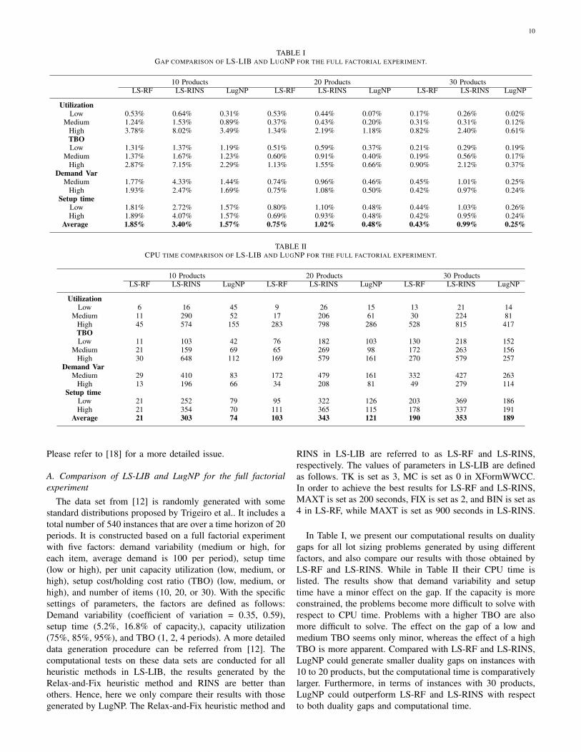
TABLE IGAP COMPARISON OF LS-LIB AND LUGNP FOR THE FULL FACTORIAL EXPERIMENT.

10 Products 20 Products 30 ProductsLS-RF LS-RINS LugNP LS-RF LS-RINS LugNP LS-RF LS-RINS LugNP

UtilizationLow 0.53% 0.64% 0.31% 0.53% 0.44% 0.07% 0.17% 0.26% 0.02%

Medium 1.24% 1.53% 0.89% 0.37% 0.43% 0.20% 0.31% 0.31% 0.12%High 3.78% 8.02% 3.49% 1.34% 2.19% 1.18% 0.82% 2.40% 0.61%TBOLow 1.31% 1.37% 1.19% 0.51% 0.59% 0.37% 0.21% 0.29% 0.19%

Medium 1.37% 1.67% 1.23% 0.60% 0.91% 0.40% 0.19% 0.56% 0.17%High 2.87% 7.15% 2.29% 1.13% 1.55% 0.66% 0.90% 2.12% 0.37%

Demand VarMedium 1.77% 4.33% 1.44% 0.74% 0.96% 0.46% 0.45% 1.01% 0.25%

High 1.93% 2.47% 1.69% 0.75% 1.08% 0.50% 0.42% 0.97% 0.24%Setup time

Low 1.81% 2.72% 1.57% 0.80% 1.10% 0.48% 0.44% 1.03% 0.26%High 1.89% 4.07% 1.57% 0.69% 0.93% 0.48% 0.42% 0.95% 0.24%

Average 1.85% 3.40% 1.57% 0.75% 1.02% 0.48% 0.43% 0.99% 0.25%

TABLE IICPU TIME COMPARISON OF LS-LIB AND LUGNP FOR THE FULL FACTORIAL EXPERIMENT.

10 Products 20 Products 30 ProductsLS-RF LS-RINS LugNP LS-RF LS-RINS LugNP LS-RF LS-RINS LugNP

UtilizationLow 6 16 45 9 26 15 13 21 14

Medium 11 290 52 17 206 61 30 224 81High 45 574 155 283 798 286 528 815 417TBOLow 11 103 42 76 182 103 130 218 152

Medium 21 159 69 65 269 98 172 263 156High 30 648 112 169 579 161 270 579 257

Demand VarMedium 29 410 83 172 479 161 332 427 263

High 13 196 66 34 208 81 49 279 114Setup time

Low 21 252 79 95 322 126 203 369 186High 21 354 70 111 365 115 178 337 191

Average 21 303 74 103 343 121 190 353 189

Please refer to [18] for a more detailed issue.

A. Comparison of LS-LIB and LugNP for the full factorialexperiment

The data set from [12] is randomly generated with somestandard distributions proposed by Trigeiro et al.. It includes atotal number of 540 instances that are over a time horizon of 20periods. It is constructed based on a full factorial experimentwith five factors: demand variability (medium or high, foreach item, average demand is 100 per period), setup time(low or high), per unit capacity utilization (low, medium, orhigh), setup cost/holding cost ratio (TBO) (low, medium, orhigh), and number of items (10, 20, or 30). With the specificsettings of parameters, the factors are defined as follows:Demand variability (coefficient of variation = 0.35, 0.59),setup time (5.2%, 16.8% of capacity,), capacity utilization(75%, 85%, 95%), and TBO (1, 2, 4 periods). A more detaileddata generation procedure can be referred from [12]. Thecomputational tests on these data sets are conducted for allheuristic methods in LS-LIB, the results generated by theRelax-and-Fix heuristic method and RINS are better thanothers. Hence, here we only compare their results with thosegenerated by LugNP. The Relax-and-Fix heuristic method and

RINS in LS-LIB are referred to as LS-RF and LS-RINS,respectively. The values of parameters in LS-LIB are definedas follows. TK is set as 3, MC is set as 0 in XFormWWCC.In order to achieve the best results for LS-RF and LS-RINS,MAXT is set as 200 seconds, FIX is set as 2, and BIN is set as4 in LS-RF, while MAXT is set as 900 seconds in LS-RINS.

In Table I, we present our computational results on dualitygaps for all lot sizing problems generated by using differentfactors, and also compare our results with those obtained byLS-RF and LS-RINS. While in Table II their CPU time islisted. The results show that demand variability and setuptime have a minor effect on the gap. If the capacity is moreconstrained, the problems become more difficult to solve withrespect to CPU time. Problems with a higher TBO are alsomore difficult to solve. The effect on the gap of a low andmedium TBO seems only minor, whereas the effect of a highTBO is more apparent. Compared with LS-RF and LS-RINS,LugNP could generate smaller duality gaps on instances with10 to 20 products, but the computational time is comparativelylarger. Furthermore, in terms of instances with 30 products,LugNP could outperform LS-RF and LS-RINS with respectto both duality gaps and computational time.

11

TABLE IIICOMPARISON OF LS-RF, LS-RINS, AND LUGNP

LS-RF LS-RINS LugNPLB UB D-Gap Time UB D-Gap Time UB D-Gap Time

Tr6-15(G30) 37,103.1 37,996.9 2.41% 3 38,595.7 4.02% 2 37,809 1.90% 10Tr6-30(G62) 60,946.2 61,907 1.58% 10 62,340 2.29% 235 61,746 1.31% 111Tr12-15(G53) 73,848.0 74,754 1.23% 10 75,348 2.03% 15 74,634 1.06% 10Tr12-30(G69) 130,177.2 130,711 0.41% 19 130,859 0.52% 15 130,596 0.32% 182Tr24-15(G57) 136,365.7 136,537 0.13% 12 136,840 0.35% 14 136,509 0.11% 50Tr24-30(G72) 287,753.4 288,163 0.14% 26 288,112 0.12% 12 287,937 0.06% 106

*Note that LB denotes lower bounds, UB denotes upper bounds, and D-Gap indicates duality gaps.

TABLE IVCOMPARISON OF LS-RF, CPLEX, AND LUGNP FOR HARD INSTANCES.

LS-RF-G LS-RF-T CPLEX-G CPLEX-T LugNP-G LugNP-T

TBOLow 18.79% 1185 13.66% 3000 8.13% 871

Medium 13.65% 1164 6.68% 3000 5.78% 884High 7.19% 977 4.63% 3000 3.05% 983

Demand VarMedium 15.21% 1512 9.29% 3000 6.06% 1223

High 11.22% 704 7.37% 3000 5.25% 602Setup time

Low 6.77% 930 6.45% 3000 3.45% 829High 19.66% 1287 10.20% 3000 7.86% 996

Average 13.22% 1108 8.33% 3000 5.66% 912*Note that -G indicates the duality gap for the corresponding methods, and -T denotes the computational time correspondingly.

B. Comparison of LugNP, LS-RF, and LS-RINS with OtherData Sets

Compared to LS-RF and LS-RINS, LugNP would providesmaller duality gaps. For more comparisons, we take sixprominent instances taken from a test set used by [12]. InTable III, we make a comparison on LS-RF and LS-RINS andour proposed LugNP algorithm. Although we cannot make avery robust conclusion based on such a limited comparison, theresults of gap improvements show that LugNP could achievemuch better solution qualities with a comparatively largercomputational time.

C. More Results and Comparisons on Hard Instances

From the computational results presented above, LugNPis able to reduce the duality gaps substantially further whencompared to several other heuristic algorithms used in LS-LIB. Here we would like to present computational results onhard problems that have a high capacity utilization. We pickout some hard problems from the full factorial experimentgenerated by Trigeiro et al. [12]. These hard problems have30 items and 20 periods with high capacity utilization. Slightchanges are made to the settings of parameters for theseproblems to make them harder, both parameters of setup costsand setup times for all items and periods are multiplied by 4.Table IV shows the comparison results among LS-RF, CPLEX,and LugNP. Only results from LS-RF are listed here becauseit obtains the best results among all heuristic methods in LS-LIB. From the results, we know that LugNP has a betterperformance when compared with LS-RF and CPLEX withrespect to both duality gaps and computing time, and thatLugNP is especially suitable for hard instances.

VI. CONCLUSION AND FUTURE RESEARCH

In this paper, we propose a new LugNP approach for thecapacitated multi-item lot sizing problem with setup times.In the hybrid approach we combine three approaches, NestedPartitions, Column Generation, and Relax-and-Fix togetherto solve the problem efficiently. To achieve strong lowerbounds, we formulate the problem into the classical FLformulation, which is known to provide strong lower bounds.We propose a Dantzig-Wolfe Decomposition reformulation ofthe FL formulation, and a Column Generation algorithm isimplemented to solve its LP relaxation problem, which isable to provide a strong lower bound and a good guidanceon Nested Partitions in the hybrid approach. A time-orienteddecomposition heuristic, Relax-and-Fix, is also proposed inthe hybrid approach to obtain a good initial Promising Regionand speed up the algorithm. Computational results show thatthe LugNP approach provides good results for the CLST. Alimited comparison suggests that it is superior to a state-of-the-art system, LS-LIB, and a commercial MIP solver, CPLEX 10.Extensions of this research can focus on both the reformulationand the algorithm. Many extensions of the lot sizing problemhave been proposed, such as the overtime allowance case,the backlogging case, the shortage allowance case, and themultilevel production case. It would be interesting to adaptour proposed hybrid approach to all of these extensions.

ACKNOWLEDGMENT

This research was supported in part by the National ScienceFoundation under grant CMMI-00646697, and by the AirForce Office of Scientific Research under grant FA9550-07-1-0390.

12

REFERENCES

[1] T.J. Barany, V. Roy, and L.A. Wolsey, ”Uncapacitated lot sizing: Theconvex hull of solutions,” Mathematical Programming Study, vol. 43, no.10, pp. 22-32, 1984.

[2] Y. Pochet and L.A. Wolsey, ”Solving multi-item lot-sizing problems usingstrong cutting planes,” Management Science, vol. 37, no. 1, pp. 53-67,1991.

[3] L.A. Wolsey, ”Integer Programming,” John Wiley & Sons, Inc, 1998.[4] A.J. Miller, G.L. Nemhauser, and M.W.P. Savelsbergh, ”On the polyhedral

structure of a multi-item production planning model with setup times,”Mathematical Programming, vol. 94, no. 2-3, pp. 375-405, 2003.

[5] J. Krarup and O. Bilde, ”Plant location, set covering and economiclotsizes: An O(mn) algorithm for structured problems,” Optimierung beiGraphentheoretischen und Ganzzahligen Probleme, BirkhauserVerlag, pp.155-180, 1977.

[6] G.D. Eppen and R.K. Martin, ”Solving multi-item capacitated lot-sizingproblems using variable redefinition,” Operations Research, vol. 35, no.6, pp. 832-848, 1987.

[7] H. Stadtler, ”Reformulations of the shortest route model for dynamicmulti-item multi-level capacitated lotsizing,” OR Spectrum, vol. 19, no.2, pp. 87-96, 1997.

[8] M. Florian, J.K. Lenstra, and H.G.K. Rinnooy, ”Deterministic productionplanning: Algorithms and complexity,” Management Science. vol. 26, no.7, pp. 669-679, 1980.

[9] G. Belvaux and L.A. Wolsey, ”bc-prod: A specialized branch-and-cutsystem for lot-sizing problems,” Management Science, vol. 46, no. 5, pp.724-738, 2000.

[10] A. Federgruen, M. Joern, and T. Michal, ”Progressive interval heuristicsfor multi-item capacitated lot-sizing problems,” Operations Research, vol.55, no. 3, pp. 490-502, 2007.

[11] Z. Degraeve and R. Jans, ”A new Dantzig-Wolfe reformulation andbranch-and-price algorithm for the capacitated lot-sizing problem withsetup times,” Operations Research, vol. 55, no. 5, pp. 909-920, 2007.

[12] W. Trigeiro, L.J. Thomas, and O.M. John, ”Capacitated lot sizing withsetup times,” Management Science, vol. 35 no. 3, pp. 353-366, 1989.

[13] H. Tempelmeier and M. Derstroff, ”A lagrangian-based heuristic fordynamic multilevel multiitem constrained lotsizing with setup times,”Management Science, vol. 42, no. 5, pp. 738-757, 1996.

[14] M. Salomon, ”Deterministic lot sizing models for production planning,”Spinger, Inc, 1991.

[15] N.C. Simpson and S.S. Erenguc, ”Modeling multiple stage manufactur-ing systems with generalized costs and capacity issues,” Naval ResearchLogistics, vol. 52, no. 6, pp. 560-570, 2005.

[16] F. Sahling, L. Buschkuhl, H. Tempelmeier, and S. Helber, ”Solving amulti-level capacitated lot sizing problem with multi-period setup carry-over via a fix-and-optimize heuristic,” Computers & Operations Research,vol. 36, no. 9, pp. 2546-2553, 2009.

[17] N. Absi and S. Kedad-Sidhoum, ”MIP-based heuristics for multi-itemcapacitated lot-sizing problem with setup times and shortage costs,”RAIRO-Operations Research, vol. 41, no. 2, pp. 171-192, 2007.

[18] Y. Pochet, M. Van Vyve, and L.A. Wolsey, ”LS-LIB: A library oftools for solving production planning problems,” Research Trends inCombinatorial Optimization, pp. 317-346, 2009.

[19] L. Shi and S. Olafsson, ”Nested partitions method for global optimiza-tion,” Operations Research, vol. 48, no. 3, pp. 390-407, 2000.

[20] L. Shi, S. Olafsson, and N. Sun, ”New parallel randomized algorithmsfor the traveling salesman problem,” Computers & Operations Research,vol. 26, pp. 371-394, 1999.

[21] L. Shi, S. Olafsson, and Q. Chen, ”An optimization framework forproduct design,” Management Science, vol. 47, no. 12, pp. 1681-1692,2001.

[22] L. Pi, Y. Pan, and L. Shi, ”Hybrid nested partitions and mathematicalprogramming approach and its applications,” IEEE transaction on Au-tomation Science and Engineering, vol. 5, no. 4, pp. 573-586, 2008.

[23] D. Aksen, K. Altinkemer, and S. Chand, ”The single-item lot-sizingproblem with immediate lost sales,” European Journal of OperationalResearch, vol. 147, no. 3, pp. 558-566, 2003.

[24] F. Vanderbeck and M.W.P. Savelsbergh, ”A generic view of Dantzig-Wolfe decomposition in mixed integer programming,” Operation ResearchLetters, vol. 34, no. 3, pp. 296-306, 2006.

[25] A.S. Manne, ”Programming of Economic Lot Sizes,” ManagementScience, vol. 4, no. 2, pp. 115-135, 1958.

[26] H. Stadtler, ”Multilevel lot sizing with setup times and multiple con-strained resources: internally rolling schedules with lot-sizing windows,”Operations Research, vol. 51, no. 3, pp. 487-506, 2003.

Tao Wu received his undergraduate degree fromMechanical Engineering at Nanchang University in2001, his master degree from Mechanical Engineer-ing at Chongqing University in 2005, his masterdegrees from Industrial Engineering and ComputerSciences at University of Wisconsin-Madison in2006 and 2009, respectively, and his Ph.D degreefrom Industrial and Systems Engineering at Uni-versity of Wisconsin-Madison in 2010. He is nowworking at Meda Engineering as a research engi-neer, but assigned to R&D at General Motors. His

research interests are in the arena of building mathematical, analytical, andstatistical models, and developing algorithms, methodologies, and theories forsolving real industrial problems. His work has been applied in manufacturingsystems, data mining, process control, production planning, and supplychain management. The work has appeared or is forthcoming in Journalof Global Optimization, Annals of Operations Research, European Journalof Operational Research, Computers & Operations Research, InternationalJournal of Production Research, IEEE Trans. on Automation Science andEngineering, and Journal of Systems Science and Systems Engineering.

Leyuan Shi is a Professor with Department ofIndustrial and Systems Engineering at Universityof Wisconsin-Madison. She received her Ph.D inApplied Mathematics from Harvard Universityin 1992, her M.S in Engineering from HarvardUniversity in 1990, her M.S in Applied Mathematicsfrom Tsinghua University in 1985, and her B.S inMathematics from Nanjing Normal University in1982. Dr. Shi has been involved in undergraduateand graduate teaching, as well as research andprofessional service. Dr. Shi’s research is devoted

to the theory and applications of large-scale optimization algorithms, discreteevent simulation and modeling and analysis of discrete dynamic systems. Shehas published many papers in these areas. Her work has appeared in DiscreteEvent Dynamic Systems, Operations Research, Management Science, IEEETrans., and IIE Trans. She is currently a member of the editorial board forJournal of Manufacturing & Service Operations Management, and is anAssociate Editor of Journal of Discrete Event Dynamic Systems. Dr. Shi isa member of IEEE and INFORMS.

Neil A. Duffie is a Professor with Department ofMechanical Engineering at University of Wisconsin-Madison. He received his Ph.D in Mechanical En-gineering from University of Wisconsin-Madisonin 1980, his M.S in Mechanical Engineering fromUniversity of Wisconsin-Madison in 1974, and hisB.S in Mechanical Engineering from University ofWisconsin-Madison in 1972. Professor Duffie’s re-search in manufacturing systems involves integratingsensors, actuators, computers and data bases intoadvanced automated production systems. He has

developed controls for self-guided inspection machines and welding robots,high-performance material handling systems, and automated finishing systemsfor mold and die production and rework. He is studying highly distributed,non-hierarchical system control architectures in hope of reducing cost andcomplexity in large-scale, computer-controlled manufacturing systems whileincreasing flexibility and fault tolerance.