Verma & Sharma, Cogent Engineering (2015), 2: 1008861http://dx.doi.org/10.1080/23311916.2015.1008861

PRODUCTION & MANUFACTURING | RESEARCH ARTICLE

Lagrangian based approach to solve a two level capacitated lot sizing problemMayank Verma1,2* and R.R.K. Sharma1

Abstract: Two-level, multi-item, multi-period-capacitated dynamic lot-sizing prob-lem with inclusions of backorders and setup times, TL_CLSP_BS, a well-known NP-hard problem, is solved using a novel procedure. Lagrangian relaxation of the material balance constraint reduces TL_CLSP_BS to a single-constraint continu-ous knapsack problem. Reduced problem is solved using bounded variable linear programs (BVLPs). We obtain promising bounds, which provides a better start to the branch-and-bound procedure. Limited empirical investigations are carried out on four problem sizes. In terms of computational time, the developed procedure is efficient than the CPLEX solver of GAMS. Further, while GAMS could not solve the largest problem size considered here, our procedure could solve the same in around one second time. This clearly highlights the efficacy of the developed procedure. The solution technique is applicable to any problem structure, which is reducible to the application of BVLPs.

Subjects: Operations Research; Production Systems; Manufacturing & Processing; Supply Chain Management

Keywords: multi-level; lot sizing; Lagrangian; knapsack; bounded variable linear program

*Corresponding author: Mayank Verma, Department of Industrial & Management Engineering, Indian Institute of Technology Kanpur, Kanpur 208 016, India; Scientific Officer, Atomic Energy Regulatory Board, Mumbai, IndiaE-mail: mayankverma.p@gmail.com

Reviewing editor:Zude Zhou, Wuhan University of Technology, China

Additional information is available at the end of the article

ABOUT THE AUTHORSMayank Verma is a PhD in Operations Research from the Indian Institute of Technology Kanpur. He is currently working as a scientific officer with the Indian Atomic Energy Regulatory Board.

R.R.K. Sharma is a professor of Management at the Department of Industrial and Management Engineering, Indian Institute of Technology Kanpur. He is a PhD in Management from the Indian Institute of Management Ahmedabad. He has 20+ years of teaching and research experience and published around 80 papers in international/national journals and reputed conference proceedings. He has also authored a book on MRP systems.

PUBLIC INTEREST STATEMENTA two-level-, multi-item-, multi-period-capacitated dynamic lot-sizing problem with inclusions of backorders and setup times—TL_CLSP_BS—a well-known NP-hard problem, is solved using a novel procedure. Lagrangian relaxation of the material balance constraint reduces TL_CLSP_BS to a single-constraint continuous knapsack problem. Reduced problem is solved using bounded variable linear programs. We obtain promising bounds, which provides a better start to the branch-and-bound procedure. Limited empirical investigations are carried out on four problem sizes. In terms of computational time, the developed procedure is efficient than the CPLEX solver of GAMS. Further, while GAMS could not solve the largest problem size considered here, our procedure could solve the same in around one second time. This clearly highlights the efficacy of the developed procedure. The solution technique is applicable to any problem structure, which is reducible to the application of bounded variable linear programs.

Received: 21 May 2014Accepted: 12 January 2015Published: 13 February 2015

© 2015 The Author(s). This open access article is distributed under a Creative Commons Attribution (CC-BY) 4.0 license.

Page 1 of 13

Page 2 of 13

Verma & Sharma, Cogent Engineering (2015), 2: 1008861http://dx.doi.org/10.1080/23311916.2015.1008861

1. IntroductionTo create a production plan over a finite number of periods, where the demand has to be fulfilled while facing finite capacities is known to be a difficult problem. It is even harder in case of a multi-level product structure, where items are related to each other by successor–predecessor relation-ship, as per the bill of material. For the dynamic multi-item multi-level-capacitated lot-sizing problem (ML_CLSP_BS) considered here, the following assumptions apply (Maes, McClain, & Van Wassenhove, 1991):

(1) A general two-level product structure is present, without loops in the bill of material.

(2) The planning horizon is divided into a number of periods.

(3) Items with dynamic external demands are arranged in the product structure.

(4) Inventory holding costs are computed based on the end-of-period inventory.

(5) Backorders are allowed and have a backorder cost.

(6) Once an item is produced, a fixed setup time and a fixed setup cost occur in addition to vari-able production cost.

(7) The objective is to minimize the sum of holding costs, setup costs, backorder costs, and the variable production costs.

There had been studies addressing the solution to a multi-level CLSP in the past, but certain real-istically relevant variables were excluded to simplify the solution procedure. Billington, McClain, and Thomas (1986) consider a general product structure and Billington, Blackburn, Maes, Millen, and Van Wassenhove (1994) assume a linear product structure with uniform processing times; they however did not consider the setup times. Maes and Van Wassenhove (1986) and Maes et al. (1991) devel-oped heuristics for the case of linear product structure, where capacity is not shared in between different levels. Kuik, Salomon, Van Wassenhove, and Maes (1993) worked on a linear product struc-ture, for which only a capacitated level exists among multiple levels, they too did not consider setup times. Tempelmeier and Helber (1994) then developed a heuristic for the case of a general product structure, where multiple resources share their capacities by items appearing in different levels of the product structure. Tempelmeier and Derstroff (1996) applied Lagrangian relaxation, França, Armentano, Berretta, and Clark (1997) developed a heuristic procedure, and Segerstedt (1996) used dynamic programming for the general product structure with setup times. Recent reviews of mod-eling and solution approaches of lot-sizing problems are provided by Drexl and Kimms (1997), Karimi, Fatemi Ghomi, and Wilson (2003) and Jans and Degraeve (2007). Other recent works on multi-level lot-sizing problems are Tempelmeier and Buschkühl (2009), Sahling, Buschkuhl, Tempelmeier, and Helber (2009), Han, Tang, Kaku, and Mu (2008), Pitakaso, Almeder, Doerner, and Hartl (2004), and Dellaert and Jeunet (2003).

This paper has attempted a two-level-capacitated lot-sizing problem. Some of the recent litera-tures on two-level lot-sizing problems are Melo and Wolsey (2010) and Toledo, Arantes, and França (2011).

In Section 2, we discuss the formulation of multi-level CLSP_BS. Section 3 explains a two-level product structure and formulates two-level CLSP_BS by modifying the formulation of multi-level CLSP_BS. In Section 4, the Lagrangian relaxation is applied to the formulation of TL_CLSP_BS and the problem reduces to a knapsack problem. Section 5 details the solution procedure for the reduced knapsack problem. Section 6 provides the computational details of the described approach. Finally, the work and its significance is concluded in Section 7.

2. FormulationBasic formulation structure of a multi–level-capacitated lot-sizing problem is borrowed from the literature (Özdamar & Barbarosoglu, 2000; Stadtler, 1996; Tempelmeier & Derstroff, 1996). The model is suitably adapted for the considered variables and situations.

Page 3 of 13

Verma & Sharma, Cogent Engineering (2015), 2: 1008861http://dx.doi.org/10.1080/23311916.2015.1008861

Decision variables

XPit number of items “i” to be produced during the period “t”XINVit number of items “i” carried as inventory at the end of period “t”XBOit number of items “i” that will be backordered from period “t”YSit binary variable for setup of the resource for item “i” during the period “t” ∈ {0, 1} i.e. 0

(if there is no setup required), 1 otherwise

Parameters

CPit unit cost of producing item “i” in period “t”CSit unit cost of setup, for item “i” in period “t”CINVit unit cost of holding inventory of item “i” for 1 periodCBOit unit cost of Backordering item “i”, which was demanded during the period “t”CAPit capacity available to produce item “i” during the period “t” CAPTt capacity available in time units, in a period “t”Dit external demand of item “i” during the period “t”TPi time required to process the item “i”TSi time required to setup the production for item “i”Si set of successors of item “i” in the product structureNij number of items “i” required to produce 1 unit of its successor “j” in the product structure

Index used in the model

i, j item, i = 1, … , I; j ∈ Si

t planning period, t = 1, … , T

Formulation of multi-level-capacitated lot-sizing problem with considerations of backorders and setup times (ML_CLSP_BS) is given as follows:

subject to:

Equation 1 gives the objective function intending to minimize the production, setup, inventory, and backorders cost, summed over all items and time periods. Equation 2 is the material balance con-straint for each item and time period.

∑j∈SiXPjtNij represents the internal demand of a non-end item

(1)Min Z =∑

i

∑

t

{CPitXPit + CSitYSit + CINVitXINVit + CBOitXBOit

}

(2)XPit + XINVi,t−1 + XBOit = Dit + XINVit + XBOi,t−1 +∑

j∈Si

XPjtNij ∀i,t

(3)∑

i=1

(TPiXP

it+ TS

iYS

it) ≤ CAPT

t∀t

(4)XPit≤ CAP

itYS

it∀i, t

(5)XPit≥ 0 ∀i, t

(6)XINVit, XBO

it≥ 0 ∀i, t

(7)XINVi0, XINViT , XBOi0, XBOi,T = 0 ∀i

(8)YSit∈ [0, 1] ∀i, t

Page 4 of 13

Verma & Sharma, Cogent Engineering (2015), 2: 1008861http://dx.doi.org/10.1080/23311916.2015.1008861

“i,” for the production of next level of item “j.” Refer Figure 1 for a better idea about connection between levels of “i” and “j.” Also note that non-end items may have an external demand in addition to the demand that is generated by its successor (internal demand); hence the presence of Dit is justified for non-end items too. Equation 3 is the time capacity constraint ensuring that the total time utilized in doing production of all the items is always less than or equal to the maximum time available in any period. Equation 4 is the production capacity constraint, which ensures the produc-tion quantity to be always less than or equal to the maximum production capacity available for all items and time periods. Equation 5 is the non-negativity restriction. Equations 6 and 7 assumes that there are no initial or final inventory and backorders. Equation 8 enforces binary restriction on the setup variables. The setup variable is equal to one when setup takes place for an item in a period, otherwise zero.

3. Two-level problem formulationFigure 2 is a typical example of the product structure with four items in two levels, showing the suc-cessor–predecessor relationship. Item 1 is the end item or the final assembly, for which an external demand would be known as a result of the forecast. Items 2, 3, and 4 are the non-end items or the intermediate sub-assemblies, required in 6, 4, and 8 numbers, respectively, to produce one unit of Item 1.

For the two-level product structure, constraint (2) can be written as:

Equation 2′ is true for end as well as non-end items in a two-level product structure. So, formulation of TL_CLSP_BS is given by P: Minimize Equation 1, subject to Equations 2′, and 3–8.

4. Relaxation and reductionIt is evident from the formulation of the TL_CLSP_BS that Equation 2 is the only constraint that links the two levels of the product structure. Equation 2 is relaxed using Lagrangian procedure to solve a two-level version of the problem.

(2′)XPit + XINVi,t−1 + XBOit = Dit + XINVit + XBOi,t−1 + XP1tNi1 ∀i,t

Figure 2. A two-level product structure. 1

(1)

2 (6)

3 (4)

4 (8)

Level 1

Level 2

Figure 1. Relation between the two levels of product structure.

End Items

Raw Materials

N

j

i ii

Page 5 of 13

Verma & Sharma, Cogent Engineering (2015), 2: 1008861http://dx.doi.org/10.1080/23311916.2015.1008861

4.1. Relaxing material balance constraintWe use an unrestricted Lagrangian multiplier λ2it to relax (2), an equality constraint. The problem (P2) takes the following shape for a TL_CLSP_BS.

P2:

Subject to: (Equations 3–8).

4.2. Reduction to continuous knapsack problemTo solve P2, we temporarily omit the term Ditλ2it, λ2itXP1tNi1 and also the terms containing inventory and backorder variables. The problem takes the following shape:

Subject to: (Equations 3–5) and (Equation 8).

Note that the omission of some terms at this step is just to make the problem structure amenable to application of the bounded variable linear program (BVLP) solution procedure. The terms omitted now will be included back to the solution procedure at an appropriate step, so that the intent of their presence in the problem structure is not lost. Equation 4 gives an upper bound (=CAPit) on the value of the production variable XPit. If a procedure can take care of this upper bound in its steps, we can eliminate Equation 4 from the problem structure. The problem now takes a special structure of a single-constraint continuous knapsack problem (Pk) for each time period “t”, where the variable XPit has an upper bound (=CAPit).

This single-constraint continuous knapsack problem can be solved efficiently using the concept of BVLP as described in the following section.

5. Solution procedureWe now devise a very efficient and easy to implement solution scheme using BVLP (Murty, 1976). BVLP is solved inside the iterations of sub-gradient optimization. This is detailed out as follows.

5.1. Determining production and setup variablesThe procedure starts with sub-gradient optimization by assuming an initial value for the Lagrangian multipliers. We arrange the set (i, t) in the sequence of ascending ratio of the term CPit−�2it

TPi

. In this order of (i, t), we replace XPit by its upper bound CAPit till the right-hand resource is available. All XPit, which remain unallocated, are made zero. For each set of (i, t), we now determine the sense (nega-tive or positive) of the term [(CPit − �2it)XPit + CSit]. For those set of (i, t), for which the term is nega-tive, we make YSit = 1; and for all other (i, t), we make YSit = 0.

In case of two-level problems, capacities of the second-level items are substantially higher, when compared to its individual demand Dit, where i ∈ {2, I}. Because of this, the lower bounds obtained with these values of XPit (=CAPit) may be higher than the optimal solution. It is hence necessary to

(9)

Max�2

MinXP, YS, XINV, XBO

Z2=

I∑i=1

T∑t=1

�(CP

it− �2

it)XP

it+ CS

itYS

it+ D

it�2

it+ �2

itXP

1tNi1

(CINVit+ �2

it)XINV

it− (�2

it)XINV

i,t−i+ (CBO

it− �2

it)XBO

it+ (�2

it)XBO

i,t−1

�

⎫⎪⎬⎪⎭

(10)Max�2

MinXP,YS

Z2=

I∑

i=1

T∑

t=1

[(CP

it− �2

it)XP

it+ CS

itYS

it

]

(11)Pk: Max�2

MinXP,YS

Z2 =

I∑

i=1

T∑

t=1

[(CPit − �2it)XPit + CSitYSit

]

(3)Subject to

I∑

i=1

(TPiXPit + TSiYSit

)≤ CAPTt ∀t

Page 6 of 13

Verma & Sharma, Cogent Engineering (2015), 2: 1008861http://dx.doi.org/10.1080/23311916.2015.1008861

adjust the values of XPit i ∈ {2, I}. The values of XPit i ∈ {2, I} are reduced from CAPit to the range [(Range of Dit) × T) + (Range of CAP1t) × (Range of Nij)].

5.2. Inventory and backorder variablesWe now get back the values of inventory and backorder variables, which were lost due to the proce-dure of Lagrangian relaxation and BVLPs.

Let �_INVit = CINVit + �2it − �2i,t+1 and �_BOit = CBOit − �2it + �2i,t+1. If α_BOit  <  0 and α_INVit  >  0, we assign XBOit = |XPit  −  Dit| and XINVit  =  0. If α_BOit  >  0 and α_INVit  <  0, we assign XINVit = |XPit − Dit| and XBOit = 0. In case both α_BOit < 0 and α_INVit < 0, the term corresponding to the lower of the two is assigned a magnitude equal to |XPit  −  Dit|; that is, if α_INVit  <  α_BOit, assign XINVit = |XPit − Dit| and XBOit = 0, otherwise XBOit = |XPit − Dit| and XINVit = 0. Similar is the case if both α_BOit > 0 and α_INVit > 0, we then allocate a zero value to both variables XBOit = 0 and XINVit = 0.

In this way, we now have determined the values of XPit, YSit, λ2it, XINVit, and XBOit. We start the sub-gradient optimization iterations to update the value of λ2it. At each iteration of the sub-gradient optimization procedure, we have an updated λ2it, and hence a correspondingly updated XPit, YSit, XINVit, and XBOit. Continue sub-gradient iterations till the improvement is very less (say < 0.001). At the end of sub-gradient iterations, we have the final updated values of XPit, YSit, λ2it, XINVit, XBOit that are used to obtain the value of the “lower bound”.

5.3. Determining upper boundIn Section 5.2, in order to determine the variables using BVLPs, we may have ended up getting an infeasible solution. To obtain an upper bound, we modify the solution to obtain a feasible solution. Constraints (3–8) are all taken care by the procedure and only constraint left out is Equation 2, which was relaxed using a Lagrangian multiplier. Mathematically,

∑tXP

it=∑

tDit;∀i, if inventory and

backorders are to be zero at the start and end of the planning horizon. But the total quantity of an item produced over the complete planning horizon (all time periods) is not equal to the total quan-tity of that item in demand over all time periods, due to the used procedure. This causes infeasibility, which needs to be appropriately dealt with.

In order to find a feasible solution (upper bound), we check if ∑

t XPit >∑

t Dit, then XPit is reduced where CPit is maximum; till either XPit = Dit or

∑t XPit =

∑t Dit is satisfied. In case if

∑t XPit <

∑t Dit,

increase XPit for the time period for which CPit is minimum; till either XPit = CAPit or ∑

t XPit =∑

t Dit is satisfied. After doing this adjustment, we move period by period from the first time period, for which Dit and XPit are both known. If XPit − Dit is positive, it indicates an overproduction and hence an inven-tory will be carried. Otherwise, the negative value of XPit − Dit suggests that a backorder is to be car-ried. In this way, we obtain the values of XINVi1 and XBOi1 by observing the sense (negative or positive) of the term XPit − Dit, and numerically equal to |XPit − Dit|.

From the second period to all the subsequent periods, we watch the sense of the term XP

it+ XINV

i,t−1− D

it− XBO

i,t−1 to be positive or negative. A positive value of this term implies an

inventory; else, a negative value means the backorders to be carried. The values of respective inven-tory and backorder variables is given by |XP

it+ XINV

i,t−1− D

it− XBO

i,t−1|.

So now, we get the values of production, setup, inventory, and backorder variables, which can be substituted in the problem “P” to obtain its objective value, which is the “feasible solution” or the “upper bound.” In later part of this paper, this upper bound obtained is referred to as the “Initial” solution obtained by “Procedure”.

5.4. Improvement by branch and boundWe apply branch-and-bound procedure to search the better solutions and prune the branches con-taining inferior solutions. We use the upper bound obtained above (referred as “current best” in the enumeration procedure) and the lower bound obtained at the end of sub-gradient optimization pro-cedure as the root node of the search tree and then do branching on this root node.

Page 7 of 13

Verma & Sharma, Cogent Engineering (2015), 2: 1008861http://dx.doi.org/10.1080/23311916.2015.1008861

At root node, we have obtained the initial best solution keeping all the binary setup variables free to take any value (0 or 1). As we move forward, we consider the binary variables one by one and start to fix their value to 0 or 1. The solution procedure is applied keeping these binary variables fixed at each branch. If the solution obtained at a branch is better than the “current best,” it is updated with this solution, else the branch is pruned. We keep moving from one node to the other by branching on the binary variables and keeping the previous binary variable fixed at which we obtained a better “current best” solution. In this way, all binary variables are considered one by one; the procedure is stopped when all branches are explored or pruned and all binary variables are fixed to either 0 or 1. At the end of this enumeration procedure, we obtain the “current best” feasible solution to the prob-lem CLSP_BS, which is either equal to the optimal solution or acts as an upper bound to the optimal solution with very low duality gap.

The efficacy of this procedure is checked by implementing it through the developed computer codes on a variety of randomly generated problem sets of different sizes. In later part of this paper (Section 6), this upper bound obtained is referred to as the “After Enumeration” solution obtained by “Procedure”.

5.5. Minimum cost network flow problemMinimum cost network flow (MCF) problem is solved by obtaining information about the value of setup variables from the procedure discussed in previous sub-sections. In this way, MCF provides us with yet another and a very good upper bound (feasible solution). When MCF is solved on the values of setup variables obtained in “Initial” procedure, the solution thus obtained is called “Initial” solu-tion obtained from MCF. Also during enumeration, at each node, as soon as we get the information about the value of setup variables, a MCF problem is thus solved. The solution so obtained at the end of this enumeration is called “After Enumeration” solution of MCF. It is expected that MCF will give very promising duality gaps in shorter computational times.

6. Computational experiencesTo check the performance of the solution procedure described in the previous section, the computa-tional experiments on the randomized data-sets are performed. The procedure was coded in C and run on 2.40 GHz, 3.87 GB RAM, 64-bit operating system, Intel (R) Core (TM) i5 CPU M 450 stand-alone PCs. Initially, the code was developed in MATLAB, but after running those codes, it was realized that MATLAB was only marginally efficient, when compared with the GAMS performance. As this was against our expectations, we proceed to test a single common routine written in MATLAB and also in C. It was observed that to get the same output, the computational time taken by MATLAB is 6–20 times that of C. The reason to this inefficiency of MATLAB is probably due to its large overheads, that C does not possess. Therefore, we moved on to convert the developed MATLAB code into C; the results given in this paper are hence those obtained by the C code only.

6.1. DataThe cost parameters used in the formulation is generated by coding a random generator in C lan-guage. We choose uniform distribution to generate parameters which is widely used in the literature of CLSP for this purpose. The following Table 1 states the range of values of different parameters that are taken to form the random problems.

Table 1. Range of parametersParameter Range Parameter RangeCINV_CLit U (10, 20) TPi U (50, 80)

CBO_CLit U (20, 30) TSi U (250, 300)

CSit U (500, 600) Dit U (20, 30)

CPit U (80, 100) CAP1t U (25, 35)

Nij U (1, 10) CAPit for i ∈ {2, I} U (250, 300)

Page 8 of 13

Verma & Sharma, Cogent Engineering (2015), 2: 1008861http://dx.doi.org/10.1080/23311916.2015.1008861

It is clear from Table 1 that we assume backorder costs to be higher as compared to the inventory carrying costs, as backorder costs also account for the loss of goodwill for the customer, who could not be served instantly. It also implies that our model is comparatively more open to inventory as compared to the backorders, as prompt satisfaction of the demand is primarily important in today’s competitive environment. Also, setup costs are considerably larger as compared to the production cost; similarly, setup time is assumed notably larger than the production time.

Range of the randomly generated values of demand and production capacity almost overlap each other, but the upper and lower limits of capacity is assumed slightly higher than that of demand, so that the scope of inventory is ensured in the model while at the same time allowing backorders too when demand is more than the production capacity. The relation between demand and production capacity can also be stated in terms of tightness factor, which can be defined as the ratio of average periodic demand and production capacity. For an uncapacitated problem, the value of tightness fac-tor will be 0; while for the case when required capacity is exactly equal to the available capacity, the tightness factor is 1. As one can observe that for the data considered in this work, the tightness fac-tor is roughly about 0.8. With such a rigid tightness factor, it is possible that some infeasible prob-lems are generated, such infeasible problems however are selectively eliminated from the problem sets.

6.2. Time complexityComplexity of a mixed-integer programming problem is hard to measure mathematically, as it depends on many factors for a given model. Hence, experimental approach to determine the com-plexity is the most favorable and adopted practical indicator. Though number of variables (integer/continuous) and constraints may not necessarily correspond to the computing burden, we provide a summary of the four sizes of problems considered to show the relationships. Number of constraints and variables in the problem are a fair indicator of the computational time. While the number of binary variables is of the order (IT), the order of continuous variables is (3IT) and the number of con-straints is (2IT + T).

As the problem size grows, number of variables and constraints increase. Note that the sizes (5 × 10 and 10 × 5) are almost the same as far as the number of binary and continuous variables is considered; there is, however, a change in the number of constraints for the two sizes. It would be interesting to note the relative behavior of these sizes with each other, when we compare their aver-age computational times on the same platform and similar problems (Table 2).

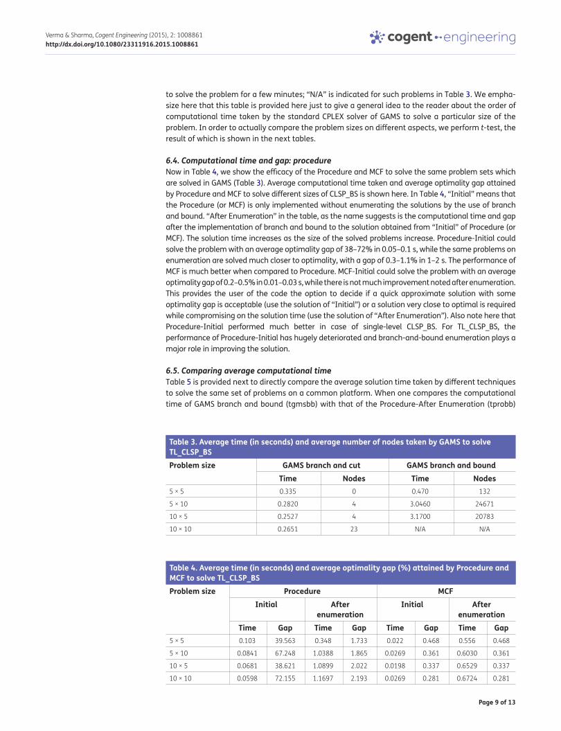
6.3. Computational time and nodes: GAMSNext in Table 3, we note the average computational time and the number of nodes taken by GAMS to solve the problems of various sizes, using the method of branch and bound and also branch and cut. One may note that as the problem size increases, the computational time as well as the number of nodes increases. Also, it is noted that branch and cut is much more efficient when compared to branch and bound. All problem sizes considered in this work are solvable by branch and cut within a second; however, computational time using branch and bound is 3–4 s. For small-sized problems, while branch and bound appears to be more efficient than branch and cut, as problem size grows, computational time of branch and bound grows to the order of around 4 s. For further large-sized problems, branch and bound cease to perform at all, as the solver went out of memory after trying

Table 2. Model statistics—number of variables and constraints in different formulationsProblem size Binary variables Continuous variables Constraints5 × 5 25 75 55

5 × 10 50 150 110

10 × 5 50 150 105

10 × 10 100 300 210

Page 9 of 13

Verma & Sharma, Cogent Engineering (2015), 2: 1008861http://dx.doi.org/10.1080/23311916.2015.1008861

to solve the problem for a few minutes; “N/A” is indicated for such problems in Table 3. We empha-size here that this table is provided here just to give a general idea to the reader about the order of computational time taken by the standard CPLEX solver of GAMS to solve a particular size of the problem. In order to actually compare the problem sizes on different aspects, we perform t-test, the result of which is shown in the next tables.

6.4. Computational time and gap: procedureNow in Table 4, we show the efficacy of the Procedure and MCF to solve the same problem sets which are solved in GAMS (Table 3). Average computational time taken and average optimality gap attained by Procedure and MCF to solve different sizes of CLSP_BS is shown here. In Table 4, “Initial” means that the Procedure (or MCF) is only implemented without enumerating the solutions by the use of branch and bound. “After Enumeration” in the table, as the name suggests is the computational time and gap after the implementation of branch and bound to the solution obtained from “Initial” of Procedure (or MCF). The solution time increases as the size of the solved problems increase. Procedure-Initial could solve the problem with an average optimality gap of 38–72% in 0.05–0.1 s, while the same problems on enumeration are solved much closer to optimality, with a gap of 0.3–1.1% in 1–2 s. The performance of MCF is much better when compared to Procedure. MCF-Initial could solve the problem with an average optimality gap of 0.2–0.5% in 0.01–0.03 s, while there is not much improvement noted after enumeration. This provides the user of the code the option to decide if a quick approximate solution with some optimality gap is acceptable (use the solution of “Initial”) or a solution very close to optimal is required while compromising on the solution time (use the solution of “After Enumeration”). Also note here that Procedure-Initial performed much better in case of single-level CLSP_BS. For TL_CLSP_BS, the performance of Procedure-Initial has hugely deteriorated and branch-and-bound enumeration plays a major role in improving the solution.

6.5. Comparing average computational timeTable 5 is provided next to directly compare the average solution time taken by different techniques to solve the same set of problems on a common platform. When one compares the computational time of GAMS branch and bound (tgmsbb) with that of the Procedure-After Enumeration (tprobb)

Table 4. Average time (in seconds) and average optimality gap (%) attained by Procedure and MCF to solve TL_CLSP_BSProblem size Procedure MCF

Initial After enumeration

Initial After enumeration

Time Gap Time Gap Time Gap Time Gap5 × 5 0.103 39.563 0.348 1.733 0.022 0.468 0.556 0.468

5 × 10 0.0841 67.248 1.0388 1.865 0.0269 0.361 0.6030 0.361

10 × 5 0.0681 38.621 1.0899 2.022 0.0198 0.337 0.6529 0.337

10 × 10 0.0598 72.155 1.1697 2.193 0.0269 0.281 0.6724 0.281

Table 3. Average time (in seconds) and average number of nodes taken by GAMS to solve TL_CLSP_BSProblem size GAMS branch and cut GAMS branch and bound

Time Nodes Time Nodes5 × 5 0.335 0 0.470 132

5 × 10 0.2820 4 3.0460 24671

10 × 5 0.2527 4 3.1700 20783

10 × 10 0.2651 23 N/A N/A

Page 10 of 13

Verma & Sharma, Cogent Engineering (2015), 2: 1008861http://dx.doi.org/10.1080/23311916.2015.1008861

and MCF-After Enumeration (tmcfbb), the efficacy of the developed algorithms is indubitably illus-trated. While for the largest sized problems, GAMS branch and bound went out of memory, “Procedure” could solve the problem in around 1 s and “MCF” solved the problem in around 0.6 s. For problem size 10 × 5, GAMS branch and bound solved the problem in around 3 s, but Procedure and MCF after enumeration could solve the problem closer to optimality in around (or less than) 1 s. The computational time taken by Procedure-Initial (tproin) and MCF-Initial (tmcfin) are shown here to compare with the computational time of GAMS branch and cut (tgmsbc), which is probably one of the fastest solving techniques available commercially. While for the largest sized problems, GAMS branch and cut took around 0.28 s to solve the problem, “Procedure-Initial” and “MCF-Initial” could solve the problem (of course with some optimality gap) in around 50th fraction of a second. This clearly highlights the efficacy of the developed algorithms. Though, however, Procedure-Initial and MCF-Initial used for the computation of the upper bounds were there to provide a starting point to the branch-and-bound procedure, it actually generated reasonably good bounds.

6.6. Comparing computational time and optimality gap of different problem sizesIn Table 6, we show the t-test results comparing the computational times and the optimality gaps of the different size problems. This is done to statistically compare the observations of one size with the other. Note that in the following table, against 5 × 10–5 × 5 row, the column “tgmsbb” or “tgmsbc” indicates the “t” calculated for difference between the GAMS branch-and-cut computational times of (5 × 10/5 × 5) and 1; and “tgmsbb” is the “t” calculated for difference between GAMS branch-and-bound computational time for 5 × 10/5 × 5 and 1. Similarly, for “tproin,” “gproin,” “tprobb,” “tmcfin,” “gmcfin,” “tmcfbb,” and all other rows of the table. The t values in Table 6 are compared with the t-critical values given in Table 7 to determine the significance. One may note that in general, the computational time increases as the size of problem increases. Similarly the optimality gap; smaller problems are solved much closer to optimality as compared to the large-sized problems. That is, smaller the problem, efficient is the procedure devised in this work to solve that problem. Note that

Table 5. Average computational time taken by different methods to solve the same set of 20 problems for each sizeSize tgmsbc tgmsbb tproin tprobb tmcfin tmcfbb5 × 5 0.335 0.470 0.103 0.348 0.022 0.556

5 × 10 0.2820 3.0460 0.0841 1.0388 0.0269 0.6030

10 × 5 0.2527 3.1700 0.0681 1.0899 0.0198 0.6529

10 × 10 0.2651 N/A 0.0598 1.1697 0.0269 0.6724

Notes: tgmsbc: Computational time taken by GAMS using branch and cut.tgmsbb: Computational time taken by GAMS using branch and bound.tproin: Computational time taken by procedure, without branch and bound.tprobb: Computational time taken by procedure, with branch and bound.tmcfin: Computational time taken by MCF, without branch and bound.tmcfbb: Computational time taken by MCF, with branch and bound.

Table 6. t values comparing computational times and optimality gaps of different-sized problemsCompare size tgmsbc tgmsbb tproin gproin tprobb gprobb tmcfin gmcfin tmcfbb gmcfbb5 × 10–5 × 5 0.12 2.43 0.37 13.5 4.71 1.55 2.13 0.47 1.42 0.47

10 × 10–10 × 5 2.0 N/A 0.03 15.15 2.33 1.022 3.52 1.45 1.6 1.45

10 × 5–5 × 5 −0.84 2.75 −1.64 −0.46 1.9 1.48 1.04 0.36 1.7 0.36

10 × 10–5 × 10 1.33 N/A −1.47 2.94 1.74 1.31 1.83 1.04 2.08 1.04

Notes: gproin: Optimality gap at the end of procedure, without branch and bound.gprobb: Optimality gap at the end of procedure, with branch and bound.gmcfin: Optimality gap at the end of MCF, without branch and bound.gmcfbb: Optimality gap at the end of MCF, with branch and bound.

Page 11 of 13

Verma & Sharma, Cogent Engineering (2015), 2: 1008861http://dx.doi.org/10.1080/23311916.2015.1008861

against some columns, we have few negative values, for example, the row 10 × 5–5 × 5. This means that statistically the optimality gap obtained by Procedure-Initial of size 5 × 5 is more than that of the size 5 × 10. Similar is the explanation for other rows/columns with a negative value. “N/A” in the third column (tgmsbb) indicates that the computational time to solve one or both of these problems is not available as the solver went out of memory.

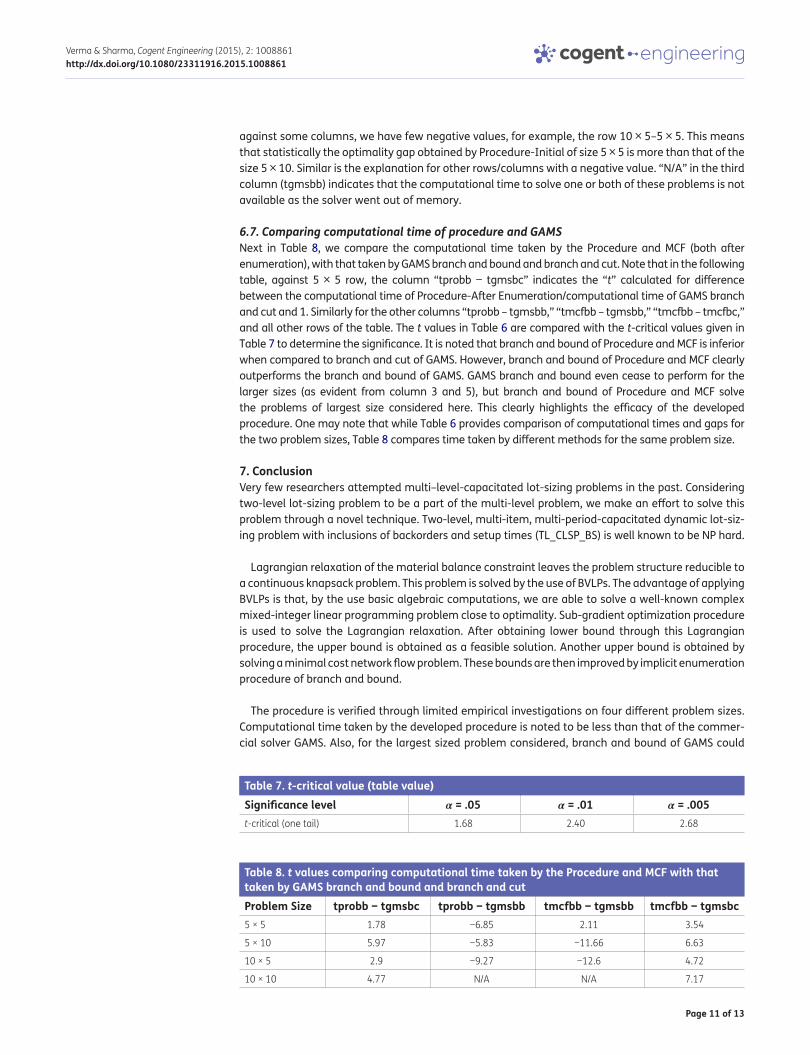
6.7. Comparing computational time of procedure and GAMSNext in Table 8, we compare the computational time taken by the Procedure and MCF (both after enumeration), with that taken by GAMS branch and bound and branch and cut. Note that in the following table, against 5  ×  5 row, the column “tprobb  −  tgmsbc” indicates the “t” calculated for difference between the computational time of Procedure-After Enumeration/computational time of GAMS branch and cut and 1. Similarly for the other columns “tprobb – tgmsbb,” “tmcfbb – tgmsbb,” “tmcfbb – tmcfbc,” and all other rows of the table. The t values in Table 6 are compared with the t-critical values given in Table 7 to determine the significance. It is noted that branch and bound of Procedure and MCF is inferior when compared to branch and cut of GAMS. However, branch and bound of Procedure and MCF clearly outperforms the branch and bound of GAMS. GAMS branch and bound even cease to perform for the larger sizes (as evident from column 3 and 5), but branch and bound of Procedure and MCF solve the problems of largest size considered here. This clearly highlights the efficacy of the developed procedure. One may note that while Table 6 provides comparison of computational times and gaps for the two problem sizes, Table 8 compares time taken by different methods for the same problem size.

7. ConclusionVery few researchers attempted multi–level-capacitated lot-sizing problems in the past. Considering two-level lot-sizing problem to be a part of the multi-level problem, we make an effort to solve this problem through a novel technique. Two-level, multi-item, multi-period-capacitated dynamic lot-siz-ing problem with inclusions of backorders and setup times (TL_CLSP_BS) is well known to be NP hard.

Lagrangian relaxation of the material balance constraint leaves the problem structure reducible to a continuous knapsack problem. This problem is solved by the use of BVLPs. The advantage of applying BVLPs is that, by the use basic algebraic computations, we are able to solve a well-known complex mixed-integer linear programming problem close to optimality. Sub-gradient optimization procedure is used to solve the Lagrangian relaxation. After obtaining lower bound through this Lagrangian procedure, the upper bound is obtained as a feasible solution. Another upper bound is obtained by solving a minimal cost network flow problem. These bounds are then improved by implicit enumeration procedure of branch and bound.

The procedure is verified through limited empirical investigations on four different problem sizes. Computational time taken by the developed procedure is noted to be less than that of the commer-cial solver GAMS. Also, for the largest sized problem considered, branch and bound of GAMS could

Table 7. t-critical value (table value)Significance level α = .05 α = .01 α = .005t-critical (one tail) 1.68 2.40 2.68

Table 8. t values comparing computational time taken by the Procedure and MCF with that taken by GAMS branch and bound and branch and cutProblem Size tprobb − tgmsbc tprobb − tgmsbb tmcfbb − tgmsbb tmcfbb − tgmsbc5 × 5 1.78 −6.85 2.11 3.54

5 × 10 5.97 −5.83 −11.66 6.63

10 × 5 2.9 −9.27 −12.6 4.72

10 × 10 4.77 N/A N/A 7.17

Page 12 of 13

Verma & Sharma, Cogent Engineering (2015), 2: 1008861http://dx.doi.org/10.1080/23311916.2015.1008861

not solve the problem and went out of memory, while through the developed procedure, the same problem could be solved in around 1 s time. This clearly highlights the efficacy of the developed procedure. The solution technique is applicable to any problem, the structure of which is amenable or reducible to the application of BVLPs.

As a future research, we propose to apply the procedure developed in this work to multi-level prob-lems, which are much closer to reality. Also, while improving the solution by implicit enumeration procedure, branch and cut may be used instead of branch and bound, which is observed to be the better performer.

FundingThis work was done as a part of the PhD thesis of Dr Mayank Verma.

Author detailsMayank Verma1,2

E-mail: mayankverma.p@gmail.comR.R.K. Sharma1

E-mail: rrks@iitk.ac.in1 Department of Industrial & Management Engineering,

Indian Institute of Technology Kanpur, Kanpur 208 016, India.

2 Scientific Officer, Atomic Energy Regulatory Board, Mumbai, India.

Citation informationCite this article as: Lagrangian based approach to solve a two level capacitated lot sizing problem, Mayank Verma & R.R.K. Sharma, Cogent Engineering (2015), 2: 1008861.

ReferencesBillington, P. J., Blackburn, J., Maes, J., Millen, R., & Van

Wassenhove, L. N. (1994). Multi-item lotsizing in capacitated multi-stage serial systems. IIE Transactions, 26, 12–18. http://dx.doi.org/10.1080/07408179408966591

Billington, P. J., McClain, J. O., & Thomas, L. J. (1986). Heuristics for multilevel lot sizing with a bottleneck. Management Science, 32, 989–1006.

Dellaert, N. P., & Jeunet, J. (2003). Randomized multi-level lot-sizing heuristics for general product structures. European Journal of Operational Research, 148, 211–228. http://dx.doi.org/10.1016/S0377-2217(02)00403-4

Drexl, A., & Kimms, A. (1997). Lot sizing and scheduling—Survey and extensions. European Journal of Operational Research, 99, 221–235. http://dx.doi.org/10.1016/S0377-2217(97)00030-1

França, P. M., Armentano, V. A., Berretta, R. E., & Clark, A. R. (1997). A heuristic method for lot sizing in multi-stage systems. Computers and Operations Research, 24, 861–874. http://dx.doi.org/10.1016/S0305-0548(96)00097-4

Han, Y., Tang, J., Kaku, I., & Mu, L. (2008). Solving uncapacitated multilevel lot-sizing problems using a particle swarm optimization with flexible inertial weight. Computers and Mathematics with Applications, 57, 1748–1755. doi:10.1016/j.camwa.2008.10.024

Jans, R., & Degraeve, Z. (2007). Meta-heuristics for dynamic lot sizing: A review and comparison of solution approaches. European Journal of Operational Research, 177, 1855–1875. http://dx.doi.org/10.1016/j.ejor.2005.12.008

Karimi, B., Fatemi Ghomi, S. M., & Wilson, J. M. (2003). The capacitated lot sizing problem: A review of models and algorithms. Omega, 31, 365–378. http://dx.doi.org/10.1016/S0305-0483(03)00059-8

Kuik, R., Salomon, M., Van Wassenhove, L. N., & Maes, J. (1993). Linear programming, simulated annealing and tabu search heuristics for lot sizing in bottleneck assembly systems. IIE Transactions, 11, 319–326.

Maes, J., McClain, J. O., & Van Wassenhove, L. N. (1991). Multilevel capacitated lotsizing complexity and LP-based heuristics. European Journal of Operational Research, 53, 131–148. http://dx.doi.org/10.1016/0377-2217(91)90130-N

Maes, J., & Van Wassenhove, L. N. (1986). A simple heuristic for the multi item single level capacitated lotsizing problem. Operations Research Letters, 4, 265–273. http://dx.doi.org/10.1016/0167-6377(86)90027-1

Melo, R. A., & Wolsey, L. A. (2010). Uncapacitated two-level lot-sizing. Operations Research Letter, 38, 241–245.

Murty, K. G. (1976). Bounded variable linear programs. In K. G. Murty (Ed.), Linear and combinatorial programming (pp. 271–287). Wiley.

Özdamar, L., & Barbarosoglu, G. (2000). An integrated Lagrangean relaxation-simulated annealing approach to the multi-level multi-item capacitated lot sizing problem. International Journal of Production Economics, 68, 319–331. http://dx.doi.org/10.1016/S0925-5273(99)00100-0

Pitakaso, R., Almeder, C., Doerner, K. F., & Hartl, R. F. (2004). Combining population-based and exact methods for multi-level capacitated lot-sizing problems. International Journal of Production Research, 44, 4755–4771.

Sahling, F., Buschkuhl, L., Tempelmeier, H., & Helber, S. (2009). Solving a multi-level capacitated lotsizing problem with multi-period setup carry-over via a fix-and-optimize heuristic. Computers & Operations Research, 36, 2546–2553.

Segerstedt, A. (1996). A capacity-constrained multi-level inventory and production control problem. International Journal of Production Economics, 45, 449–461. http://dx.doi.org/10.1016/0925-5273(96)00017-5

Stadtler, H. (1996). Mixed integer programming model formulations for dynamic multi-item multi-level capacitated lotsizing. European Journal of Operational Research, 94, 561–581. http://dx.doi.org/10.1016/0377-2217(95)00094-1

Tempelmeier, H., & Buschkühl, L. (2009). A heuristic for the dynamic multi-level capacitated lotsizing problem with linked lotsizes for general product structures. OR Spectrum, 31, 385–404. http://dx.doi.org/10.1007/s00291-008-0130-y

Tempelmeier, H., & Derstroff, M. (1996). A Lagrangean-based heuristic for dynamic multilevel multiitem constrained lotsizing with setup times. Management Science, 42, 738–757. http://dx.doi.org/10.1287/mnsc.42.5.738

Tempelmeier, H., & Helber, S. (1994). A heuristic for dynamic multi-item multi-level capacitated lotsizing for general product structures. European Journal of Operational Research, 75, 296–311. http://dx.doi.org/10.1016/0377-2217(94)90076-0

Toledo, C. F., Arantes, M. S., & França, P. M. (2011). Tabu search to solve the synchronized and integrated two-level lot sizing and scheduling problem. In 13th Annual Genetic and Evolutionary Computation Conference, GECCO 2011, Proceedings. Dublin, Ireland. doi:10.1145/2001576.2001638

Page 13 of 13

Verma & Sharma, Cogent Engineering (2015), 2: 1008861http://dx.doi.org/10.1080/23311916.2015.1008861

© 2015 The Author(s). This open access article is distributed under a Creative Commons Attribution (CC-BY) 4.0 license.You are free to: Share — copy and redistribute the material in any medium or format Adapt — remix, transform, and build upon the material for any purpose, even commercially.The licensor cannot revoke these freedoms as long as you follow the license terms.

Under the following terms:Attribution — You must give appropriate credit, provide a link to the license, and indicate if changes were made. You may do so in any reasonable manner, but not in any way that suggests the licensor endorses you or your use. No additional restrictions You may not apply legal terms or technological measures that legally restrict others from doing anything the license permits.

Cogent Engineering (ISSN: 2331-1916) is published by Cogent OA, part of Taylor & Francis Group. Publishing with Cogent OA ensures:• Immediate, universal access to your article on publication• High visibility and discoverability via the Cogent OA website as well as Taylor & Francis Online• Download and citation statistics for your article• Rapid online publication• Input from, and dialog with, expert editors and editorial boards• Retention of full copyright of your article• Guaranteed legacy preservation of your article• Discounts and waivers for authors in developing regionsSubmit your manuscript to a Cogent OA journal at www.CogentOA.com