eindhoven university of technology master a robust ... · abstract in this thesis the capacitated...
TRANSCRIPT
Eindhoven University of Technology
MASTER
A robust optimization approach to the capacitated lot sizing problem
van Pelt, T.D.
Award date:2015
DisclaimerThis document contains a student thesis (bachelor's or master's), as authored by a student at Eindhoven University of Technology. Studenttheses are made available in the TU/e repository upon obtaining the required degree. The grade received is not published on the documentas presented in the repository. The required complexity or quality of research of student theses may vary by program, and the requiredminimum study period may vary in duration.
General rightsCopyright and moral rights for the publications made accessible in the public portal are retained by the authors and/or other copyright ownersand it is a condition of accessing publications that users recognise and abide by the legal requirements associated with these rights.
• Users may download and print one copy of any publication from the public portal for the purpose of private study or research. • You may not further distribute the material or use it for any profit-making activity or commercial gain
Take down policyIf you believe that this document breaches copyright please contact us providing details, and we will remove access to the work immediatelyand investigate your claim.
Download date: 16. Jul. 2018
Eindhoven, December 2015
by
Thomas Daniël van Pelt
BSc Computer Science and Engineering
Student identity number 0618184
In partial fulfilment of the requirements for the degree of
Master of Science
in Operations Management and Logistics
Supervisors
Prof.dr.ir. J.C. Fransoo, Eindhoven University of Technology
Prof.dr. A.G. de Kok, Eindhoven University of Technology
A Robust Optimization Approach to
the Capacitated Lot Sizing Problem

TUE. School of Industrial Engineering.
Series Master Theses Operations Management and Logistics
Subject headings: production planning, lot sizing, robust optimization
Contents
Abstract 5
1 Introduction 11
1.1 The Capacitated Lot Sizing Problem . . . . . . . . . . . . . . . . . . . . . . . . . . . 11
1.2 Motivation and Background . . . . . . . . . . . . . . . . . . . . . . . . . . . . . . . . 12
1.3 Problem Statement and Research Questions . . . . . . . . . . . . . . . . . . . . . . . 13
1.4 Experimental Framework . . . . . . . . . . . . . . . . . . . . . . . . . . . . . . . . . 15
1.5 Research Design and Outline of the Thesis . . . . . . . . . . . . . . . . . . . . . . . . 16
2 Models for Robust Production Planning 17
2.1 Introduction . . . . . . . . . . . . . . . . . . . . . . . . . . . . . . . . . . . . . . . . 17
2.2 Multi-Stage Decision Problems . . . . . . . . . . . . . . . . . . . . . . . . . . . . . . 18
2.3 Production Planning as Linear Optimization Problem . . . . . . . . . . . . . . . . . . 18
2.4 Static Robust Optimization Models . . . . . . . . . . . . . . . . . . . . . . . . . . . . 20
2.4.1 Introducing Uncertainty . . . . . . . . . . . . . . . . . . . . . . . . . . . . . . 20
2.4.2 A Conservative Robust Counterpart: l∞-norm . . . . . . . . . . . . . . . . . . 20
2.4.3 A Less Conservative Robust Counterpart: l1-norm . . . . . . . . . . . . . . . . 23
2.4.4 Cardinality Constrained Robust Counterpart . . . . . . . . . . . . . . . . . . . 24
2.5 On Optimality of Static Robust Optimization . . . . . . . . . . . . . . . . . . . . . . 25
2.5.1 Notes on Interval Uncertainty . . . . . . . . . . . . . . . . . . . . . . . . . . . 25
2.5.2 The Effect of Using the l∞-norm or l1-norm . . . . . . . . . . . . . . . . . . . 26
2.6 Multi-Stage Robust Optimization . . . . . . . . . . . . . . . . . . . . . . . . . . . . . 27
2.6.1 Affinely Adjustable Robust Counterpart . . . . . . . . . . . . . . . . . . . . . 27
2.6.2 Adjustable Robust Mixed-Integer Optimization . . . . . . . . . . . . . . . . . 32
2.7 Distributionally Robust Optimization . . . . . . . . . . . . . . . . . . . . . . . . . . . 33
2.8 Conclusion . . . . . . . . . . . . . . . . . . . . . . . . . . . . . . . . . . . . . . . . . 33
3 The Capacitated Lot-Sizing Problem under Demand Uncertainty 35
3.1 Introduction . . . . . . . . . . . . . . . . . . . . . . . . . . . . . . . . . . . . . . . . 35
3.2 The Deterministic Capacitated Lot Sizing Problems . . . . . . . . . . . . . . . . . . . 35
3.2.1 The Problem . . . . . . . . . . . . . . . . . . . . . . . . . . . . . . . . . . . 35
3.2.2 A Mixed Integer Programming Formulation . . . . . . . . . . . . . . . . . . . 36
3.2.3 Heuristics for the Deterministic Capacitated Lot-Sizing Problem . . . . . . . . 36
3.3 The Stochastic Capacitated Lot Sizing Problem . . . . . . . . . . . . . . . . . . . . . 38
3.3.1 The Introduction of Demand Uncertainty . . . . . . . . . . . . . . . . . . . . 38
3.3.2 An Explicit Derivation for the Expected Backlog and Inventory Level . . . . . . 40
3.3.3 Linearizing the Expected Backlog and Expected Inventory Level Functions . . . 41
3.3.4 The Approximated Stochastic Capacitated Lot Sizing Problem . . . . . . . . . 43
3.3.5 Corrigendum to the Work of Tempelmeier and Hilger (2015) . . . . . . . . . . 45
3.4 A Robust Counterpart of the Capacitated Lot Sizing Problem under Interval Uncertainty 46
3.5 Conclusion . . . . . . . . . . . . . . . . . . . . . . . . . . . . . . . . . . . . . . . . . 47
3
4 CONTENTS
4 Simulation Study 494.1 Introduction . . . . . . . . . . . . . . . . . . . . . . . . . . . . . . . . . . . . . . . . 494.2 Methodology . . . . . . . . . . . . . . . . . . . . . . . . . . . . . . . . . . . . . . . . 49
4.2.1 A Discrete-Event Simulation in a Rolling Horizon Setting . . . . . . . . . . . . 494.2.2 Simulation Framework . . . . . . . . . . . . . . . . . . . . . . . . . . . . . . 50
4.3 Experimental Design . . . . . . . . . . . . . . . . . . . . . . . . . . . . . . . . . . . . 534.4 Experimental Results . . . . . . . . . . . . . . . . . . . . . . . . . . . . . . . . . . . 53
4.4.1 Experiment 1: Setting the Stage . . . . . . . . . . . . . . . . . . . . . . . . . 534.4.2 Experiment 2: Influencing the Service Level . . . . . . . . . . . . . . . . . . . 544.4.3 Experiment 3: Relative Performance under Low and High Ratios of Demand to
Capacity . . . . . . . . . . . . . . . . . . . . . . . . . . . . . . . . . . . . . . 554.5 Conclusion . . . . . . . . . . . . . . . . . . . . . . . . . . . . . . . . . . . . . . . . . 58
5 Conclusions and Future Research 595.1 Introduction . . . . . . . . . . . . . . . . . . . . . . . . . . . . . . . . . . . . . . . . 595.2 Main Research Findings . . . . . . . . . . . . . . . . . . . . . . . . . . . . . . . . . . 59
5.2.1 Using Robust Optimization in Production Planning Models . . . . . . . . . . . 595.2.2 Deriving a Stochastic Counterpart . . . . . . . . . . . . . . . . . . . . . . . . 605.2.3 Influencing the Realized β-Service Level . . . . . . . . . . . . . . . . . . . . . 605.2.4 Relative Performance under Low and High Ratios of Demand to Capacity . . . 605.2.5 General Conclusion . . . . . . . . . . . . . . . . . . . . . . . . . . . . . . . . 61
5.3 Future Research . . . . . . . . . . . . . . . . . . . . . . . . . . . . . . . . . . . . . . 61
Bibliography 64
Summary 67
Appendices 71
A Notation and Abbreviations 73
B Mathematical Preliminaries 75B.1 From Mathematical Optimization to Linear Optimization . . . . . . . . . . . . . . . . 75B.2 Norms . . . . . . . . . . . . . . . . . . . . . . . . . . . . . . . . . . . . . . . . . . . 76B.3 Integration . . . . . . . . . . . . . . . . . . . . . . . . . . . . . . . . . . . . . . . . . 76
C Proofs of Theorems 77
Abstract
In this thesis the Capacitated Lot Sizing Problem under demand uncertainty is considered. In thisproblem production has to be planned for a single resource over a finite horizon for a fixed numberof products while being constraint by per period capacity restrictions. Costs are incurred for settingup production, holding inventory and back-orders. Based on a Mixed Integer Linear Optimizationformulation we have derived a Stochastic Counterpart that assumes demand to be normally distributedas well as a Robust Counterpart that assumes demand to range in a specified interval. The realizedservice level when using the Stochastic Counterpart can be influenced by means of a β-service levelconstraint whereas for the Robust Counterpart we can set the back-order cost and the size of thedemand interval.
Both methods were compared in a simulation study in a rolling horizon setting whereby the perperiod demands for each product are drawn from the Normal distribution. First, we fitted the rightparameters to a realized service level. Second, we assessed how these models performed under variouscircumstances. We observed that the Robust Counterpart delivers more stable service levels at lowercost when capacity decreases and demand uncertainty gets higher. In general, the Robust Counterpartis superior of the Stochastic Counterpart.
5

6 CONTENTS

Acknowledgements
The completion of this thesis would not have been possible without the help of many whom I’d like tothank. First of all I would like to express the most true and deepest gratitude of all, to my first supervisor:Prof.dr.ir. Jan Fransoo. Jan, without your guidance and advice during our always challenging meetings,it would not have been possible for me to learn so much during this beautiful process. I am more thanthankful for the knowledge you have shared during this process. Second, I would like to thank mysecond supervisor Prof.dr. Ton de Kok for the valuable remarks he made during the process and theability to learn from his knowledge too. I am looking forward to work together with you in the nextphase of my studies. Third, I would like to thank Dr.ir Joachim Arts. Joachim, thank you for beingsuch a great teacher.
I could not have started working on this thesis if it weren’t for the support and love of many others.That starts with my parents. Well, mum and dad, you now have to deal with the consequence of alwaysallowing me to ask way. It continues with my brothers who are always there for me. It is awesome tohave a bear-like brother like Robert-Jan, to grow up under the safe wings of David. And life would bea hack of a lot more boring without my long lasting friend Wouter. Dude, I value every moment wemake fun. Though, it is safe to say that I would have never came so far without the never ending loveof Laurey. Moreover, I would like to thank Gal Askenazi for the love and guidance he gave me whendiscovering the place I call home.
Of course, during my studies I met a lot of people a long the way as well. Jeroen, I would liketo thank you for the enormous amount of fun we made during class or after class by generating thiswhole new form of Bits-and-Bytes cabaret. Second, you might be resembling the living definition ofperseverance as I noted during the challenge of implementing some classification algorithm... Ellen,I truly value our friendship and will miss our long coffee breaks. Furthermore, I would like to thankMatthieu and Patrick for being friends for such a long time.
There have been some great teachers that I have met along the way as well. During my stay atthe Technion - Israel Institute of Technology, I have been able to learn from the knowledge of Prof.Yale Herer and Shimrit Shtern. Furthermore, I would like to thank Prof.dr.ir. Dick den Hertog for thevaluable remarks on the mathematics of Robust Optimization.
7

8 CONTENTS

Dedicated to the living memory of Richard Geoffrey Jeanne Brounts
9

10 CONTENTS
Chapter 1
Introduction
1.1 The Capacitated Lot Sizing Problem
In this thesis we will study the Capacitated Lot Sizing Problem (CLSP) under demand uncertainty.More specifically, we will take a Robust Optimization (RO) approach based on the work of Ben-Taland Nemirovski (1998) to deal with demand uncertainty. We will start with a thorough introductioninto the field of RO based on a basic production planning problem. It should provide solid ground toexplain our new approach to the CLSP. In a simulation study this model will be compared to two othermodels: the nominal model and its Stochastic Counterpart. The former of these assumes deterministicdemand whereas the latter assumes demand to be randomly distributed. All models will be comparedin an simulated environment in a rolling horizon setting where demand is randomly generated from aknown probability distribution.
Karimi et al. (2003) define production planning to be “the activity that considers the best useof production resources in order to satisfy production goals (satisfying production requirements andanticipating sales opportunities) over a certain period named the planning horizon”. One of the problemsin production planning is the lot sizing problem, which according to Karimi et al. (2003) revolves arounddeciding on “when and how much of a product to produce such that set-up, production and holdingcosts are minimised”. We can account the first lot sizing model to Wagner and Whitin (1958). Theyconsidered time-varying but deterministic demand without any capacity restrictions. When a capacityrestriction is introduced we get the CLSP. When demand is stationary and randomly distributed wetalk about the Stochastic Economic Lot Sizing Problem, while in case demand is non-stationary, butindependent, we talk about the Stochastic CLSP.
Production planning typically encompasses three levels of decision making: strategic, tactical andoperational. Besides that, it encompasses three time ranges for decision making: long-term, medium-term and short-term. Long-term and strategic usually revolves around deciding on the product mix tooffer or where to locate a new facility. In general, one may regard this level as one where the primefocus is on anticipating aggregate needs (Karimi et al. (2003)). Medium-term planning revolves aroundMaterial Requirements Planning and determining production plans. This is the level at which the lotsizing decision resides. The production plans are then disaggregated into day-to-day schedules and thisis the level of short-term operational planning.
The lot sizing decision can be found in many companies. Winands et al. (2011) state that it is acommon problem for glass and paper production, injection molding, metal tamping, semi-continuouschemical processes and in bulk production of consumer products. For example, Fransoo et al. (1995)describe a situation at a glass-containers manufacturing company. There exists a lot sizing decisionin this situation, because if a different colour product needs to be produced, then the temperature ofthe oven in which the glass is heated has to change, which takes fours days. These four days can beregarded as the setup time and this leads to a lot sizing decision. Hence, production has to be plannedin a optimal (or near optimal) way while costs are minimized. Since there is a trade-off in inventoryholding costs and setup costs, we do not want to produce too long as inventory builds up, nor do wewant to switch too often between producing different products as it costs money and consumes valuablecapacity.
Clearly, from a practical point of view, the CLSP is worth studying for successful operations planning
11
12 CHAPTER 1. INTRODUCTION
and control. Besides a practical motivation, there is a scientific one as well. Therefore, we will continuein the next section with providing more background on the problem as well as giving a more thoroughmotivation for taking a RO approach to the CLSP under demand uncertainty.
1.2 Motivation and Background
In the previous section we gave a brief introduction to the CLSP, its relation to other decision problemsin Operations Management and the relevance of studying the problem for practice. In this section wewill dive deeper in the background of the problem and we will motivate this research. This motivationis predominantly based on existing research in which future directions are recommended. As we willdiscuss next, the first reason for this research is that the developments in the field of RO might providebetter ways to deal with uncertainty and the second reason stems from the fact that most, if not all,of the research done on the CLSP does not perform a simulation study in which the models are run ina rolling horizon setting.
When studying literature there are two aspects of research on the CLSP that stand out: increasethe computation speed and deal with uncertainty. Both Allahverdi et al. (1999) and Jans and Degraeve(2008) state that one of the major limitations of the lot sizing problems they discuss is the assumptionof deterministic demand and their inability to deal with demand uncertainty. From the work of Belvauxand Wolsey (2001), Wolsey (2002) and Pochet and Wolsey (2006) we know that we can formulatethe CLSP as a Mixed Integer Linear Optimization (LO) problem. Now given the desire to deal withuncertainty, the questions rises if we can deal with these type of problems.
The work of Dantzig (1955) can be regarded as one of the first accounts to incorporate uncertaintyinto LO problems. This was done by letting the parameters of the LO problem belong to a uncertainbut known distribution of demand. A few years later, Wagner and Whitin (1958) proposed their famousmodel for determining ordering quantities under time-varying deterministic demand. Around that timeManne (1958) came up with a LO problem for economic lot sizing models. Dzielinksi et al. (1963)simulated the models of Manne (1958) in an uncertainty environment and observe that models thatdon’t take uncertainty explicitly into account perform reasonably well in a rolling horizon. Thereafter,attention for the subject was lost for quite a while until it was revived by the work of Soyster (1973).However, the model proposed by Soyster (1973) and others have some undesirable properties: they areeither too conservative or non-linear (Soyster (1973); Bertsimas and Sim (2004)).
However, the work of Soyster (1973) has been significantly improved later on by Ben-Tal andNemirovski (1998, 1999 and 2000). The later authors developed methodologies to deal with uncertaintyin LO problems in which conservativeness can be controlled and that are computationally tractable inmost cases. By introducing uncertainty into these problems, they become Semi-Infinite Optimizationproblems. Ben-Tal and Nemirovski show that under certain circumstances these can be rewritten intotheir so called Robust Counterpart, that are again LO problems in most cases. After the work of theaforementioned authors the field of RO was born and a lot of research followed.
For example, Bertsimas and Sim (2004) propose an approach to solve uncertain LO by means of arobust formulation that is linear and has a parameter to regulate per period the conservativeness. Thework of Bertsimas and Thiele (2006) show the usefulness of this technique by applying it to problemsin inventory theory. Furthermore, this work can be regarded as the spark that led to the widespreadattention for the use of RO. The work of Ben-Tal et al. (2004) introduces multi-stage RO. In terms ofproduction planning this would mean that instead of considering the production quantities in the nextT periods as here and now decisions, we would let the production quantities in period t depend in anaffine fashion on the realizations of demand in previous periods. Some interesting results based on thistechnique have been achieved by Ben-Tal et al. (2005) regarding retailer-supplier flexible commitmentcontracts, and Ben-Tal et al. (2009b) in relation to multi-echelon inventory theory.
Furthermore, it is worth noticing that the work of Ben-Tal et al. (2009a, pp. 4-7) illustrates theimpact of minor deviations in the nominal values of the parameters used in LO problems. In theirwork they show that even the slightest deviation from the chosen parameter might render an optimalsolution infeasible and thereby meaningless. In such situation the RO techniques show their capabilityin coming up with a more robust solution which can deal with uncertainty. All in all, it can be said thatRO became a proven technique to deal with uncertainty in Mathematical Optimization problems.
With the ascent of RO we can now distinct two different approaches to deal with uncertainty: one in
1.3. PROBLEM STATEMENT AND RESEARCH QUESTIONS 13
which uncertainty is defined by means of probability distribution and one where there is a more geometricinterpretation of uncertainty. In the former case a probability distribution is underlying demand, whilein the latter we extend the polyhedron of the solution space. There are examples of applications of theformer to the CLSP like the work of Helber et al. (2013), Rossi et al. (2015) and Tempelmeier and Hilger(2015) shows. They take the nominal CLSP as starting point and deal with it from a stochastic pointof view. This means that demand is assumed to be identically and independently normally distributed.
However, in case of taking a stochastic approach two additional complexities are introduced asWinands et al. (2011) and Ben-Tal et al. (2005) point out. The first is that in practice informationregarding the demand distribution is unavailable or hard (costly) to obtain. Second, the curse ofdimensionality might render it (computationally) impossible to consider multiple products or a realisticnumber of time periods. When taking a RO approach we do not suffer from these complexities. So,with the possibility to formulate the CLSP as a Mixed Integer LO problem, a RO approach lends itselfvery well to deal with uncertainty, while avoiding the aforementioned complexities.
The second shortcoming of previous research that we mentioned and that we want to overcomeis the fact that little is known about the performance of CLSP models in a rolling horizon setting.Dzielinksi et al. (1963) were most likely one of the first to note the importance of studying productionplanning problems in a rolling horizon and more specifically, Bookbinder and Tan (1988) in relation tolot sizing. Drexl and Kimms (1997) as well as Helber et al. (2013) mention the importance of futureresearch on simulating lot sizing problems in a rolling horizon setting. This becomes even more clearif we look at the work of Tempelmeier and Hilger (2015). The model proposed herein is run and theyonly look at the objective value and this tells us nothing on how such model would perform in practice.If we want to assess how this model would perform in practice we should conduct a simulation studyin a rolling horizon setting. We are very eager to get to know how this model would perform and forthat reason we will investigated their approach.
Above we discussed two shortcomings in present day research on the CLSP. These shortcomingsmotivate our research and we want to contribute to the field by coming up with solutions for theseshortcomings. Hence, our contributions to the field are as follows:
� We will take a novel approach based on RO to deal with demand uncertainty in the nominalCLSP. This has not been done before at the scale we will do it in this research. This step will leadto the so called Robust Counterpart of the nominal CLSP under the assumption that demand isknown to range in an interval.
� We will derive our own Stochastic Counterpart of the nominal CLSP and compare it to the oneof Tempelmeier and Hilger (2015). Contrary to before, we will now assume demand to randomlydistributed.
� We will conduct an extensive simulation study in which the various models will be compared ina rolling horizon setting. Literature is scarce, if not non-existing, on the effects of running CLSPmodels under demand uncertainty in a rolling horizon, despite the fact that in practice modelsrun in such a setting. This way we hope to shed light on the effects a rolling horizon.
In the next section we translate these contributions in a research proposition. We define the problemwe want to study and come up with related research questions.
1.3 Problem Statement and Research Questions
In this section we start by giving a more formal introduction to the CLSP. We start by expressing theproblem as a Mixed Integer LO Problem. Thereafter, we discuss relevant aspects to the problem. Incombination with the motivation of the research this will lead to the research questions.
From the description of the CLSP in the previous section it became clear that we have a trade-offbetween holding inventory or setting up production for a specific product more frequently. This trade-off should be represented in the objective function of a Mixed Integer LO formulation. Furthermore,there are some aspects to take into account. First, if demand is deterministic then the resulting lotsize will not account for any other realization of demand. Hence, we might get some back-orders if itturns out to be higher than expected in case of demand uncertainty. This means that we should allowfor negative inventory contrary to a lot of other models. Second, if we allow for negative inventory
14 CHAPTER 1. INTRODUCTION
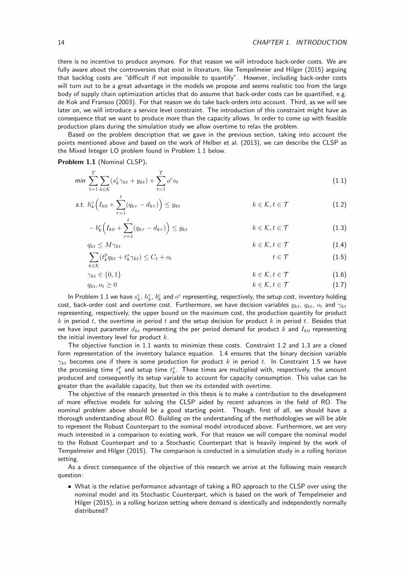
there is no incentive to produce anymore. For that reason we will introduce back-order costs. We arefully aware about the controversies that exist in literature, like Tempelmeier and Hilger (2015) arguingthat backlog costs are “difficult if not impossible to quantify”. However, including back-order costswill turn out to be a great advantage in the models we propose and seems realistic too from the largebody of supply chain optimization articles that do assume that back-order costs can be quantified, e.g.de Kok and Fransoo (2003). For that reason we do take back-orders into account. Third, as we will seelater on, we will introduce a service level constraint. The introduction of this constraint might have asconsequence that we want to produce more than the capacity allows. In order to come up with feasibleproduction plans during the simulation study we allow overtime to relax the problem.
Based on the problem description that we gave in the previous section, taking into account thepoints mentioned above and based on the work of Helber et al. (2013), we can describe the CLSP asthe Mixed Integer LO problem found in Problem 1.1 below.
Problem 1.1 (Nominal CLSP).
minT∑t=1
∑k∈K
(sckγkt + ykt) +
T∑t=1
ocot (1.1)
s.t. hck
(Ik0 +
t∑τ=1
(qkτ − dkτ ))≤ ykt k ∈ K, t ∈ T (1.2)
− bck(Ik0 +
t∑τ=1
(qkτ − dkτ ))≤ ykt k ∈ K, t ∈ T (1.3)
qkt ≤Mγkt k ∈ K, t ∈ T (1.4)∑k∈K
(tpkqkt + tskγkt) ≤ Ct + ot t ∈ T (1.5)
γkt ∈ {0, 1} k ∈ K, t ∈ T (1.6)
qkt, ot ≥ 0 k ∈ K, t ∈ T (1.7)
In Problem 1.1 we have sck, hck, bck and oc representing, respectively, the setup cost, inventory holdingcost, back-order cost and overtime cost. Furthermore, we have decision variables ykt, qkt, ot and γktrepresenting, respectively, the upper bound on the maximum cost, the production quantity for productk in period t, the overtime in period t and the setup decision for product k in period t. Besides thatwe have input parameter dkt representing the per period demand for product k and Ik0 representingthe initial inventory level for product k.
The objective function in 1.1 wants to minimize these costs. Constraint 1.2 and 1.3 are a closedform representation of the inventory balance equation. 1.4 ensures that the binary decision variableγkt becomes one if there is some production for product k in period t. In Constraint 1.5 we havethe processing time tpk and setup time tsk. These times are multiplied with, respectively, the amountproduced and consequently its setup variable to account for capacity consumption. This value can begreater than the available capacity, but then we its extended with overtime.
The objective of the research presented in this thesis is to make a contribution to the developmentof more effective models for solving the CLSP aided by recent advances in the field of RO. Thenominal problem above should be a good starting point. Though, first of all, we should have athorough understanding about RO. Building on the understanding of the methodologies we will be ableto represent the Robust Counterpart to the nominal model introduced above. Furthermore, we are verymuch interested in a comparison to existing work. For that reason we will compare the nominal modelto the Robust Counterpart and to a Stochastic Counterpart that is heavily inspired by the work ofTempelmeier and Hilger (2015). The comparison is conducted in a simulation study in a rolling horizonsetting.
As a direct consequence of the objective of this research we arrive at the following main researchquestion:
� What is the relative performance advantage of taking a RO approach to the CLSP over using thenominal model and its Stochastic Counterpart, which is based on the work of Tempelmeier andHilger (2015), in a rolling horizon setting where demand is identically and independently normallydistributed?
1.4. EXPERIMENTAL FRAMEWORK 15
In order to answer this question we will formulate the following sub questions,
1. How can we apply the methodologies of RO to production planning problems?
2. How can we derive a Stochastic Counterpart in case we take a stochastic perspective on demanduncertainty?
3. Can we formulate a Robust Counterpart for the nominal CLSP if demand is known to range in aspecified interval?
4. How should we setup an experimental framework and measure the relative performance of themodels?
5. We know that we can influence the realized β-service level in the Stochastic Counterpart by meansof a parameter. However, is the required service level equal to the realized one? If not, how canwe fit the right input to the desired output?
6. How can we influence the realized β-service level in the Robust Counterpart?
7. How much does either of the two models, the Stochastic and Robust Counterpart, perform betterthan the other under different circumstances?
These sub questions conclude this section. We have seen our motivation, research problem, objec-tives and research questions. In the next sections we will discuss the experimental framework that weuse and describe the research design.
1.4 Experimental Framework
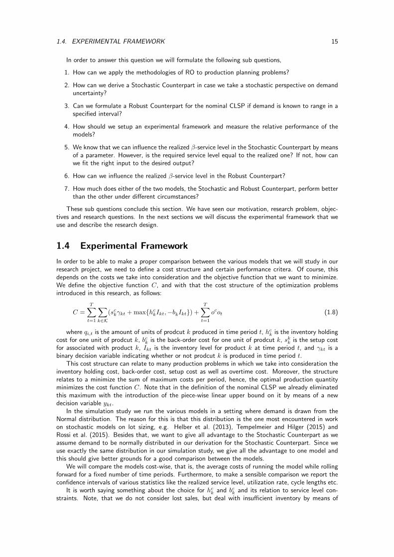
In order to be able to make a proper comparison between the various models that we will study in ourresearch project, we need to define a cost structure and certain performance critera. Of course, thisdepends on the costs we take into consideration and the objective function that we want to minimize.We define the objective function C, and with that the cost structure of the optimization problemsintroduced in this research, as follows:
C =
T∑t=1
∑k∈K
(sckγkt + max{hckIkt,−bkIkt}) +
T∑t=1
ocot (1.8)
where qi,t is the amount of units of prodcut k produced in time period t, hck is the inventory holdingcost for one unit of prodcut k, bck is the back-order cost for one unit of prodcut k, skk is the setup costfor associated with product k, Ikt is the inventory level for product k at time period t, and γkt is abinary decision variable indicating whether or not prodcut k is produced in time period t.
This cost structure can relate to many production problems in which we take into consideration theinventory holding cost, back-order cost, setup cost as well as overtime cost. Moreover, the structurerelates to a minimize the sum of maximum costs per period, hence, the optimal production quantityminimizes the cost function C. Note that in the definition of the nominal CLSP we already eliminatedthis maximum with the introduction of the piece-wise linear upper bound on it by means of a newdecision variable ykt.
In the simulation study we run the various models in a setting where demand is drawn from theNormal distribution. The reason for this is that this distribution is the one most encountered in workon stochastic models on lot sizing, e.g. Helber et al. (2013), Tempelmeier and Hilger (2015) andRossi et al. (2015). Besides that, we want to give all advantage to the Stochastic Counterpart as weassume demand to be normally distributed in our derivation for the Stochastic Counterpart. Since weuse exactly the same distribution in our simulation study, we give all the advantage to one model andthis should give better grounds for a good comparison between the models.
We will compare the models cost-wise, that is, the average costs of running the model while rollingforward for a fixed number of time periods. Furthermore, to make a sensible comparison we report theconfidence intervals of various statistics like the realized service level, utilization rate, cycle lengths etc.
It is worth saying something about the choice for hck and bck and its relation to service level con-straints. Note, that we do not consider lost sales, but deal with insufficient inventory by means of
16 CHAPTER 1. INTRODUCTION
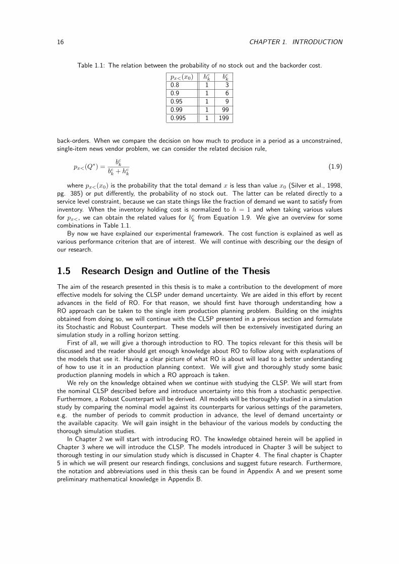
Table 1.1: The relation between the probability of no stock out and the backorder cost.
px<(x0) hck bck0.8 1 30.9 1 60.95 1 90.99 1 990.995 1 199
back-orders. When we compare the decision on how much to produce in a period as a unconstrained,single-item news vendor problem, we can consider the related decision rule,
px<(Q∗) =bck
bck + hck(1.9)
where px<(x0) is the probability that the total demand x is less than value x0 (Silver et al., 1998,pg. 385) or put differently, the probability of no stock out. The latter can be related directly to aservice level constraint, because we can state things like the fraction of demand we want to satisfy frominventory. When the inventory holding cost is normalized to h = 1 and when taking various valuesfor px<, we can obtain the related values for bck from Equation 1.9. We give an overview for somecombinations in Table 1.1.
By now we have explained our experimental framework. The cost function is explained as well asvarious performance criterion that are of interest. We will continue with describing our the design ofour research.
1.5 Research Design and Outline of the Thesis
The aim of the research presented in this thesis is to make a contribution to the development of moreeffective models for solving the CLSP under demand uncertainty. We are aided in this effort by recentadvances in the field of RO. For that reason, we should first have thorough understanding how aRO approach can be taken to the single item production planning problem. Building on the insightsobtained from doing so, we will continue with the CLSP presented in a previous section and formulateits Stochastic and Robust Counterpart. These models will then be extensively investigated during ansimulation study in a rolling horizon setting.
First of all, we will give a thorough introduction to RO. The topics relevant for this thesis will bediscussed and the reader should get enough knowledge about RO to follow along with explanations ofthe models that use it. Having a clear picture of what RO is about will lead to a better understandingof how to use it in an production planning context. We will give and thoroughly study some basicproduction planning models in which a RO approach is taken.
We rely on the knowledge obtained when we continue with studying the CLSP. We will start fromthe nominal CLSP described before and introduce uncertainty into this from a stochastic perspective.Furthermore, a Robust Counterpart will be derived. All models will be thoroughly studied in a simulationstudy by comparing the nominal model against its counterparts for various settings of the parameters,e.g. the number of periods to commit production in advance, the level of demand uncertainty orthe available capacity. We will gain insight in the behaviour of the various models by conducting thethorough simulation studies.
In Chapter 2 we will start with introducing RO. The knowledge obtained herein will be applied inChapter 3 where we will introduce the CLSP. The models introduced in Chapter 3 will be subject tothorough testing in our simulation study which is discussed in Chapter 4. The final chapter is Chapter5 in which we will present our research findings, conclusions and suggest future research. Furthermore,the notation and abbreviations used in this thesis can be found in Appendix A and we present somepreliminary mathematical knowledge in Appendix B.
Chapter 2
Models for Robust ProductionPlanning
“If a man will begin with certainties, heshall end in doubts; but if he will be contentto begin with doubts, he shall end incertainties.”
Francis Bacon, The Advancement ofLearning
2.1 Introduction
In this chapter we give an introduction into RO and explain its concepts using a basic productionplanning problem. The nominal production planning model that we present in this chapter is one forplanning production for a single item, at a single location, under a per period capacity restriction.Demand needs to be satisfied either by the end of the period in which it occurs or at a later stage whenput on back-order. This basic problem deals with the trade-off between holding inventory and acceptingback-orders. Costs are incurred for holding inventory and putting demand on back-order. Hence, theobjective of the problem is to minimize the maximum of inventory holding costs and back-order costssubject to the given constraints.
We start this chapter with discussing multi-stage decision problems in general. This should providea solid foundation for understanding the nominal production planning problem that we will introduce.This problem serves us in explaining the concepts and methodologies behind RO. Although we couldhave only referred to the numerous of introductory papers on RO, we will give a thorough introductionourself by using the nominal production planning model as starting point. Nevertheless, we couldcertainly recommend the interested reader the work of Ben-Tal et al. (2009a), Bertsimas et al. (2011)and Gorissen et al. (2015) for a more general introduction to the field.
After introducing our nominal problem, we will introduce uncertainty into it. The problem thenbecomes a semi-infinite optimization problem, which is computationally untractable. However, forspecific types of uncertainty sets we will show how to come up with tractable representations, i.e.their Robust Counterparts. The Robust Counterparts range from the most conservative to the leastconservative, one where conservatives can be controlled by means of a parameter and the AffinelyAdjustable Robust Counterpart (AARC). These Robust Counterparts can be classified under the headingof static or multi-stage RO. The former only considers “here and now” decisions, while the latter letsthe current period production quantity depend on the demand in pervious periods in an affine fashion.Using this dependency in the form of Linear Decision Rules results in the so called AARC. We concludewith a future outlook of RO and we especially discuss Distributionally RO and Multi-Stage AdjustableRobust Mixed-Integer Optimization.
17
18 CHAPTER 2. MODELS FOR ROBUST PRODUCTION PLANNING
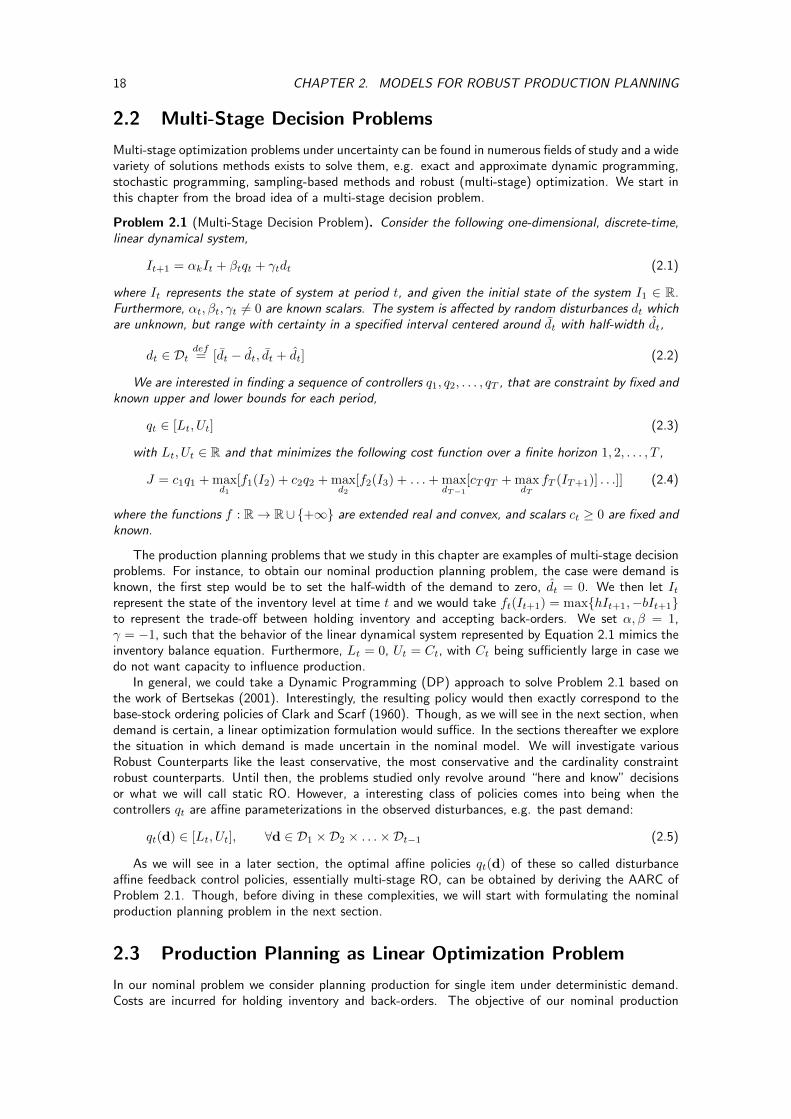
2.2 Multi-Stage Decision Problems
Multi-stage optimization problems under uncertainty can be found in numerous fields of study and a widevariety of solutions methods exists to solve them, e.g. exact and approximate dynamic programming,stochastic programming, sampling-based methods and robust (multi-stage) optimization. We start inthis chapter from the broad idea of a multi-stage decision problem.
Problem 2.1 (Multi-Stage Decision Problem). Consider the following one-dimensional, discrete-time,linear dynamical system,
It+1 = αkIt + βtqt + γtdt (2.1)
where It represents the state of system at period t, and given the initial state of the system I1 ∈ R.Furthermore, αt, βt, γt 6= 0 are known scalars. The system is affected by random disturbances dt whichare unknown, but range with certainty in a specified interval centered around dt with half-width dt,
dt ∈ Dtdef= [dt − dt, dt + dt] (2.2)
We are interested in finding a sequence of controllers q1, q2, . . . , qT , that are constraint by fixed andknown upper and lower bounds for each period,
qt ∈ [Lt, Ut] (2.3)
with Lt, Ut ∈ R and that minimizes the following cost function over a finite horizon 1, 2, . . . , T ,
J = c1q1 + maxd1
[f1(I2) + c2q2 + maxd2
[f2(I3) + . . .+ maxdT−1
[cT qT + maxdT
fT (IT+1)] . . .]] (2.4)
where the functions f : R→ R∪{+∞} are extended real and convex, and scalars ct ≥ 0 are fixed andknown.
The production planning problems that we study in this chapter are examples of multi-stage decisionproblems. For instance, to obtain our nominal production planning problem, the case were demand isknown, the first step would be to set the half-width of the demand to zero, dt = 0. We then let Itrepresent the state of the inventory level at time t and we would take ft(It+1) = max{hIt+1,−bIt+1}to represent the trade-off between holding inventory and accepting back-orders. We set α, β = 1,γ = −1, such that the behavior of the linear dynamical system represented by Equation 2.1 mimics theinventory balance equation. Furthermore, Lt = 0, Ut = Ct, with Ct being sufficiently large in case wedo not want capacity to influence production.
In general, we could take a Dynamic Programming (DP) approach to solve Problem 2.1 based onthe work of Bertsekas (2001). Interestingly, the resulting policy would then exactly correspond to thebase-stock ordering policies of Clark and Scarf (1960). Though, as we will see in the next section, whendemand is certain, a linear optimization formulation would suffice. In the sections thereafter we explorethe situation in which demand is made uncertain in the nominal model. We will investigate variousRobust Counterparts like the least conservative, the most conservative and the cardinality constraintrobust counterparts. Until then, the problems studied only revolve around “here and know” decisionsor what we will call static RO. However, a interesting class of policies comes into being when thecontrollers qt are affine parameterizations in the observed disturbances, e.g. the past demand:
qt(d) ∈ [Lt, Ut], ∀d ∈ D1 ×D2 × . . .×Dt−1 (2.5)
As we will see in a later section, the optimal affine policies qt(d) of these so called disturbanceaffine feedback control policies, essentially multi-stage RO, can be obtained by deriving the AARC ofProblem 2.1. Though, before diving in these complexities, we will start with formulating the nominalproduction planning problem in the next section.
2.3 Production Planning as Linear Optimization Problem
In our nominal problem we consider planning production for single item under deterministic demand.Costs are incurred for holding inventory and back-orders. The objective of our nominal production
2.3. PRODUCTION PLANNING AS LINEAR OPTIMIZATION PROBLEM 19
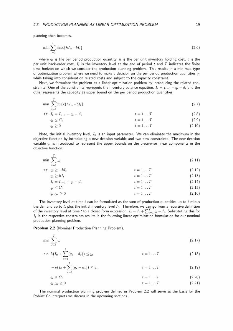
planning then becomes,
min
T∑t=1
max{hIt,−bIt} (2.6)
where qt is the per period production quantity, h is the per unit inventory holding cost, b is theper unit back-order cost, It is the inventory level at the end of period t and T indicates the finitetime horizon on which we consider the production planning problem. This results in a min-max typeof optimization problem where we need to make a decision on the per period production quantities qtwhile taking into consideration related costs and subject to the capacity constraint.
Next, we formulate the problem as a linear optimization problem by introducing the related con-straints. One of the constraints represents the inventory balance equation, It = It−1 + qt − dt and theother represents the capacity as upper bound on the per period production quantities.
minT∑t=1
max{hIt,−bIt} (2.7)
s.t. It = It−1 + qt − dt t = 1 . . . T (2.8)
qt ≤ Ct t = 1 . . . T (2.9)
qt ≥ 0 t = 1 . . . T (2.10)
Note, the initial inventory level, I0 is an input parameter. We can eliminate the maximum in theobjective function by introducing a new decision variable and two new constraints. The new decisionvariable yt is introduced to represent the upper bounds on the piece-wise linear components in theobjective function.
minT∑t=1
yt (2.11)
s.t. yt ≥ −bIt t = 1 . . . T (2.12)
yt ≥ hIt t = 1 . . . T (2.13)
It = It−1 + qt − dt t = 1 . . . T (2.14)
qt ≤ Ct t = 1 . . . T (2.15)
qt, yt ≥ 0 t = 1 . . . T (2.16)
The inventory level at time t can be formulated as the sum of production quantities up to t minusthe demand up to t, plus the initial inventory level I0. Therefore, we can go from a recursive definitionof the inventory level at time t to a closed form expression, It = I0 +
∑Tt=1 qt−dt. Substituting this for
It in the respective constraints results in the following linear optimization formulation for our nominalproduction planning problem.
Problem 2.2 (Nominal Production Planning Problem).
minT∑t=1
yt (2.17)
s.t. h(I0 +
t∑s=1
(qs − ds))≤ yt t = 1 . . . T (2.18)
− b(I0 +
t∑s=1
(qs − ds))≤ yt t = 1 . . . T (2.19)
qt ≤ Ct t = 1 . . . T (2.20)
qt, yt ≥ 0 t = 1 . . . T (2.21)
The nominal production planning problem defined in Problem 2.2 will serve as the basis for theRobust Counterparts we discuss in the upcoming sections.
20 CHAPTER 2. MODELS FOR ROBUST PRODUCTION PLANNING
2.4 Static Robust Optimization Models
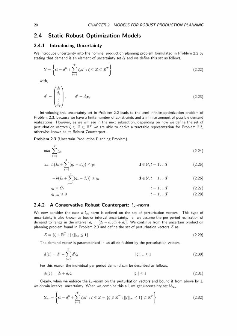
2.4.1 Introducing Uncertainty
We introduce uncertainty into the nominal production planning problem formulated in Problem 2.2 bystating that demand is an element of uncertainty set U and we define this set as follows,
U =
{d = d0 +
T∑t=1
ζtdt : ζ ∈ Z ⊂ RT
}(2.22)
with,
d0 =
d1d1...dT
, dt = dtet (2.23)
Introducing this uncertainty set in Problem 2.2 leads to the semi-infinite optimization problem ofProblem 2.3, because we have a finite number of constraints and a infinite amount of possible demandrealizations. However, as we will see in the next subsection, depending on how we define the set ofperturbation vectors ζ ∈ Z ⊂ RT we are able to derive a tractable representation for Problem 2.3,otherwise known as its Robust Counterpart.
Problem 2.3 (Uncertain Production Planning Problem).
minT∑t=1
yt (2.24)
s.t. h(I0 +
t∑s=1
(qs − ds))≤ yt d ∈ U , t = 1 . . . T (2.25)
− b(I0 +
t∑s=1
(qs − ds))≤ yt d ∈ U , t = 1 . . . T (2.26)
qt ≤ Ct t = 1 . . . T (2.27)
qt, yt ≥ 0 t = 1 . . . T (2.28)
2.4.2 A Conservative Robust Counterpart: l∞-norm
We now consider the case a l∞-norm is defined on the set of perturbation vectors. This type ofuncertainty is also known as box or interval uncertainty, i.e. we assume the per period realization ofdemand to range in the interval dt = [dt − dt, dt + dt]. We continue from the uncertain productionplanning problem found in Problem 2.3 and define the set of perturbation vectors Z as,
Z = {ζ ∈ RT : ‖ζ‖∞ ≤ 1} (2.29)
The demand vector is parameterized in an affine fashion by the perturbation vectors,
d(ζ) = d0 +
T∑t=1
dtζt ‖ζ‖∞ ≤ 1 (2.30)
For this reason the individual per period demand can be described as follows,
dt(ζ) = dt + dtζt |ζt| ≤ 1 (2.31)
Clearly, when we enforce the l∞-norm on the perturbation vectors and bound it from above by 1,we obtain interval uncertainty. When we combine this all, we get uncertainty set U∞,
U∞ =
{d = d0 +
T∑t=1
ζtdt : ζ ∈ Z = {ζ ∈ RT : ‖ζ‖∞ ≤ 1} ⊂ RT
}(2.32)
2.4. STATIC ROBUST OPTIMIZATION MODELS 21
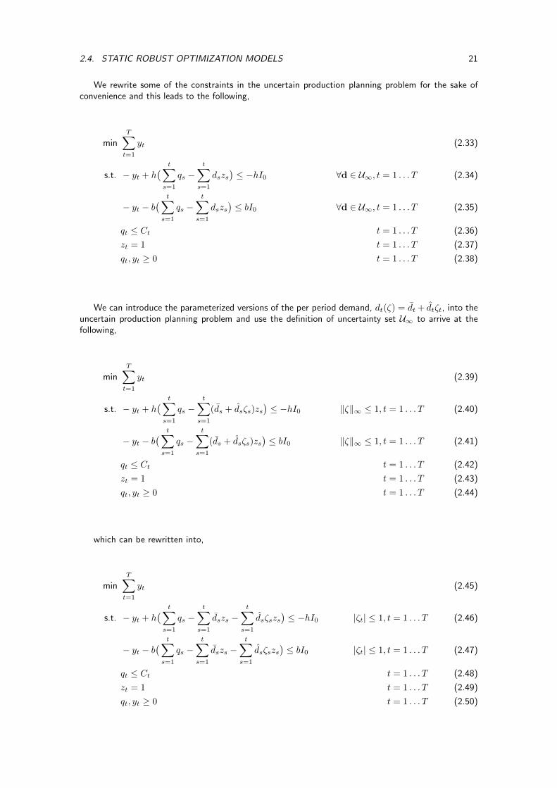
We rewrite some of the constraints in the uncertain production planning problem for the sake ofconvenience and this leads to the following,
minT∑t=1
yt (2.33)
s.t. − yt + h( t∑s=1
qs −t∑
s=1
dszs)≤ −hI0 ∀d ∈ U∞, t = 1 . . . T (2.34)
− yt − b( t∑s=1
qs −t∑
s=1
dszs)≤ bI0 ∀d ∈ U∞, t = 1 . . . T (2.35)
qt ≤ Ct t = 1 . . . T (2.36)
zt = 1 t = 1 . . . T (2.37)
qt, yt ≥ 0 t = 1 . . . T (2.38)
We can introduce the parameterized versions of the per period demand, dt(ζ) = dt + dtζt, into theuncertain production planning problem and use the definition of uncertainty set U∞ to arrive at thefollowing,
minT∑t=1
yt (2.39)
s.t. − yt + h( t∑s=1
qs −t∑
s=1
(ds + dsζs)zs)≤ −hI0 ‖ζ‖∞ ≤ 1, t = 1 . . . T (2.40)
− yt − b( t∑s=1
qs −t∑
s=1
(ds + dsζs)zs)≤ bI0 ‖ζ‖∞ ≤ 1, t = 1 . . . T (2.41)
qt ≤ Ct t = 1 . . . T (2.42)
zt = 1 t = 1 . . . T (2.43)
qt, yt ≥ 0 t = 1 . . . T (2.44)
which can be rewritten into,
minT∑t=1
yt (2.45)
s.t. − yt + h( t∑s=1
qs −t∑
s=1
dszs −t∑
s=1
dsζszs)≤ −hI0 |ζt| ≤ 1, t = 1 . . . T (2.46)
− yt − b( t∑s=1
qs −t∑
s=1
dszs −t∑
s=1
dsζszs)≤ bI0 |ζt| ≤ 1, t = 1 . . . T (2.47)
qt ≤ Ct t = 1 . . . T (2.48)
zt = 1 t = 1 . . . T (2.49)
qt, yt ≥ 0 t = 1 . . . T (2.50)
22 CHAPTER 2. MODELS FOR ROBUST PRODUCTION PLANNING
and from this, we obtain,
minT∑t=1
yt (2.51)
s.t. − yt + h( t∑s=1
qs −t∑
s=1
dszs + maxζ:‖ζ‖∞≤1
t∑s=1
dsζszs)≤ −hI0 t = 1 . . . T (2.52)
− yt − b( t∑s=1
bqs −t∑
s=1
dszs − maxζ:‖ζ‖∞≤1
t∑s=1
dsζszs ≤ bI0 t = 1 . . . T (2.53)
qt ≤ Ct t = 1 . . . T (2.54)
zt = 1 t = 1 . . . T (2.55)
qt, yt ≥ 0 t = 1 . . . T (2.56)
In general, and as a consequence of Holder’s inequality (see Appendix B), when p, q ∈ [1,∞] and1p + 1
q = 1, then the norms ‖.‖p and ‖.‖q are conjugates of each other,
‖x‖p = maxy:‖y‖q≤1
|〈x, y〉| (2.57)
We can use this to find the maximum in our constraints,
maxζ:‖ζ‖∞≤1
t∑s=1
dsζszs = maxζ:‖ζ‖∞≤1
|〈ζ, dz>〉| = ‖
d1z1d2z2
...
dszT
‖1 =
t∑s=1
|dszs| (2.58)
Therefore, using U∞ as our uncertainty set, we arrive at the following Robust Counterpart of Problem2.3,
Problem 2.4 (Robust Counterpart l∞-norm).
minT∑t=1
yt (2.59)
s.t. h(I0 +
t∑s=1
qs −t∑
s=1
dszs +
t∑s=1
ωs
)≤ yt t = 1 . . . T (2.60)
− b(I0 +
t∑s=1
qs −t∑
s=1
dszs −t∑
s=1
ωs
)≤ yt t = 1 . . . T (2.61)
− ωt ≤ dtzt ≤ ωt t = 1 . . . T (2.62)
qt ≤ Ct t = 1 . . . T (2.63)
zt = 1 t = 1 . . . T (2.64)
qt, yt ≥ 0 t = 1 . . . T (2.65)
What is of interest is the fact that when introducing uncertainty into our nominal production plan-ning problem, formulated as linear optimization problem, we got a semi-infinite optimization problemwhich in itself is intractable. However, when using interval uncertainty, we showed how to rewritethis problem to obtain a tractable formulation known as its Robust Counterpart. The beauty in thisderivation lies in the fact that its Robust Counterpart happens to be a linear optimization problemagain.
Furthermore, we see that the Robust Counterpart is indeed the most conservative approach todeal with demand uncertainty, because for each period it penalizes the constraints in the model by∑ts=1 |dszs|, being the worst-case deviation. The interested reader might find more about the conser-
vativeness in RO in the work of Gorissen and den Hertog (2013). Though, one should keep in mind,
2.4. STATIC ROBUST OPTIMIZATION MODELS 23
even though the model is conservative, as far as the objective value concerned, nothing is said by thaton how the model would perform in a simulation study in a rolling horizon setting. Moreover, as wewill see later when discussing optimality, the parameters for the inventory holding cost and back-ordercost in Problem 2.4 lend themselves very well to control the conservativeness of the model.
2.4.3 A Less Conservative Robust Counterpart: l1-norm
In the this subsection we investigate the least conservative Robust Counterpart. We will start again fromthe uncertain production planning problem of Problem 2.3. Though, now define the set of perturbationvectors as Z = {ζ ∈ RT : ‖ζ‖1 ≤ γ}. Therefore, we obtain the following uncertainty set,
U1 =
{d = d0 +
T∑t=1
ζtdt : ζ ∈ Z = {ζ ∈ RT : ‖ζ‖1 ≤ γ} ⊂ RT
}(2.66)
Analogous to what we have done in case of interval uncertainty, we can introduce the parameterizedversions of demand, dt(ζ) = dt + dtζt, into the problem and arrive at the following,
minT∑t=1
yt (2.67)
s.t. − yt +
t∑s=1
hqs − ht∑
s=1
(ds + dsζs)zs ≤ −hI0 t = 1 . . . T (2.68)
− yt −t∑
s=1
bqs + b
t∑s=1
(ds + dsζt)zs ≤ bI0 t = 1 . . . T (2.69)
qt ≤ Ct t = 1 . . . T (2.70)
zt = 1 t = 1 . . . T (2.71)
qt, yt ≥ 0 t = 1 . . . T (2.72)
which can be rewritten in the same fashion as before into,
minT∑t=1
yt (2.73)
s.t. − yt +
t∑s=1
hqs − ht∑
s=1
dszs − h maxζ:‖ζ‖1≤γ
t∑s=1
dsζszs ≤ −hI0 t = 1 . . . T (2.74)
− yt −t∑
s=1
bqs + b
t∑s=1
dszs + b maxζ:‖ζ‖1≤γ
t∑s=1
dsζszs ≤ bI0 t = 1 . . . T (2.75)
qt ≤ Ct t = 1 . . . T (2.76)
zt = 1 t = 1 . . . T (2.77)
qt, yt ≥ 0 t = 1 . . . T (2.78)
We again use the fact that the l1-norm and l∞-norm are conjugates of each other to obtain themaximum in our constraints,
maxζ:‖ζ‖1≤γ
t∑s=1
dsζszs = maxζ:‖ζ‖1≤γ
|〈ζ, dz>〉| = ‖
d1z1d2z2
...
dszT
‖∞ = γmaxs|dszs| (2.79)
Therefore, when using U1 as our uncertainty set, we arrive at the following Robust Counterpart ofProblem 2.3,
24 CHAPTER 2. MODELS FOR ROBUST PRODUCTION PLANNING
Problem 2.5 (Robust Counterpart l1-norm).
minT∑t=1
yt (2.80)
s.t. − yt +
t∑s=1
hqs − ht∑
s=1
dszs − γhmaxs:s<t
|dszs| ≤ −hI0 t = 1 . . . T (2.81)
− yt −t∑
s=1
bqs + b
t∑s=1
dszs + γbmaxs:s<t
|dszs| ≤ bI0 t = 1 . . . T (2.82)
qt ≤ Ct t = 1 . . . T (2.83)
zt = 1 t = 1 . . . T (2.84)
qt, yt ≥ 0 t = 1 . . . T (2.85)
The Robust Counterpart found in Problem 2.5 gets a penalty for robustness of γmaxs |dszs| orthe maximum deviation over all possible deviations for the planning horizon t = 1 . . . T times γ, aparameter set to be set by the decision maker. We explore this more in the one of the next subsectionwhen we compare it to the conservative Robust Counterpart.
2.4.4 Cardinality Constrained Robust Counterpart
In this section we assume cardinality constrained uncertainty and derive a robust counterpart for thenominal problem found in Problem 2.2. This type of uncertainty was first introduced by Bertsimasand Sim (2004) and gained widespread attention after showing its usefulness in a supply chain settingby Bertsimas and Thiele (2006). Other examples include the work of Alem and Morabito (2012) infurniture production and the work of Aouam and Brahimi (2013) on integrated production planningand order acceptance.
When using this type of uncertainty the per period demand dt is still assumed to range in theinterval, [dt − dt, dt + dt], though, each period the maximum allowed deviation of the center is dif-ferent and constraint from above. The set of perturbation is defined in this case as, ζ ∈ Z ={ζ ∈ RT : ‖ζ‖∞ ≤ 1 ∧
∑ts=1 |ζs| ≤ Γt
}and hence, we obtain the following uncertainty set,
Uc =
{d = d0 +
T∑t=1
ζtdt : ζ ∈ Z =
{ζ ∈ RT : ‖ζ‖∞ ≤ 1 ∧
t∑s=1
|ζs| ≤ Γt
}⊂ RT
}(2.86)
Again, demand is parameterized by the perturbation vectors, hence, dt(ζ) = dt + dtζt. We cansubstitute this in the nominal problem and obtain the following,
minT∑t=1
(cqt + yt) (2.87)
s.t. yt ≥ h
(I0 +
t∑s=1
(qs − (dt + dtζt))
)∀d ∈ Uc, t = 1 . . . T (2.88)
yt ≥ −b
(I0 +
t∑s=1
(qs − (dt + dtζt))
)∀d ∈ Uc, t = 1 . . . T (2.89)
qt ≤ Ct t = 1 . . . T (2.90)
qt, yt ≥ 0 t = 1 . . . T (2.91)
2.5. ON OPTIMALITY OF STATIC ROBUST OPTIMIZATION 25
Clearly, we have to solve the following auxiliary linear programming problem for all periods t,
maxt∑
s=1
dtζt (2.92)
s.t.t∑
s=1
ζt ≤ Γt (2.93)
0 ≤ ‖ζt‖ ≤ 1 (2.94)
Following Theorem C.1 we obtain the dual which we can substitute back in the aforementionedproblem. It readily follows that the robust counterpart is as follows,
Problem 2.6 (Robust Counterpart Cardinality Constrained Uncertainty).
minT∑t=1
(cqt + yt) (2.95)
s.t. yt ≥ h(I0 +
t∑s=1
(qs − dt) + vtΓk +
t∑i=1
rit) t = 1 . . . T (2.96)
yt ≥ b(−I0 −t∑
s=1
(qs − dt) + vtΓk +
t∑i=1
rit) t = 1 . . . T (2.97)
vt + rit ≥ di i < t, t = 1 . . . T (2.98)
vt ≥ 0 i < t, t = 1 . . . T (2.99)
rit ≥ 0 i < t, t = 1 . . . T (2.100)
qt ≤ Ct t = 1 . . . T (2.101)
2.5 On Optimality of Static Robust Optimization
2.5.1 Notes on Interval Uncertainty
Bertsimas and Thiele (2006) derive some interesting properties for the Robust Counterpart under car-dinality constraint uncertainty. In this subsection we extend them to the case of interval uncertainty.Though, we only consider the case where there are no fixed ordering costs, because we didn’t takethose into account thus far. In order to comprehend these results we have to start with the followingdefinition,
Definition 2.1 ((S,S) and (s,S) Policies, cf. Bertsimas and Thiele (2006)). The optimal policy ofan inventory optimization problem is (s, S), or base-stock, if there exists a threshold sequence (st, St)such that at each period it is optimal to let the linear dynamical system of Problem 2.1 be correctedby qt = St − dt if It < st and zero otherwise. If there is no fixed ordering cost, st = St.
This definition is essential in the theorem and corollary that we will see shortly. Below we repeat atheorem from Bertsimas and Thiele (2006) on the optimal robust policy in case of cardinality constraintuncertainty.
Theorem 2.1 (Optimal Robust Policy for Uc, cf. Bertsimas and Thiele (2006)). 1. In case ofcardinality constraint uncertainty, the optimal policy for the Robust Counterpart found in Problem2.6, evaluated at time 1 for the rest of the horizon, is the optimal policy for the nominal problemwith the modified demand,
d′t = dt +b− hb+ h
(At −At−1) (2.102)
where At = v?t Γt +∑ti=1 r
∗it is the deviation of the cumulative demand from its mean at time t,
v?t and r?it being the optimal variables in Problem 2.6.
26 CHAPTER 2. MODELS FOR ROBUST PRODUCTION PLANNING
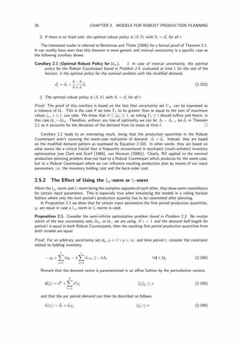
2. If there is no fixed cost, the optimal robust policy is (S, S) with St = d′t for all t.
The interested reader is referred to Bertsimas and Thiele (2006) for a formal proof of Theorem 2.1.It can readily been seen that this theorem is more generic and interval uncertainty is a specific case asthe following corollary shows.
Corollary 2.1 (Optimal Robust Policy for U∞). 1. In case of interval uncertainty, the optimalpolicy for the Robust Counterpart found in Problem 2.4, evaluated at time 1 for the rest of thehorizon, it the optimal policy for the nominal problem with the modified demand,
d′t = dt +b− hb+ h
dt (2.103)
2. The optimal robust policy is (S, S) with St = d′t for all t.
Proof. The proof of this corollary is based on the fact that uncertainty set U∞ can be expressed asa instance of Uc. This is the case if we take Γt to be greater than or equal to the sum of maximumvalues ζs, s ≤ t, can take. We know that 0 ≤ |ζt| ≤ 1, so taking Γt ≥ t should suffice and hence, inthis case Uc = U∞. Therefore, without any loss of optimality we can let At − At−1 be dt in Theorem2.1 as it accounts for the deviation of the demand from its mean at time t.
Corollary 2.1 leads to an interesting result, being that the production quantities in the RobustCounterpart aren’t covering the worst-case realization of demand: dt + dt. Instead, they are basedon the modified demand pattern as expressed by Equation 2.103. In other words, they are based onwhat seems like a critical fractal that is frequently encountered in stochastic (multi-echelon) inventoryoptimization (see Clark and Scarf (1960), van Houtum (2006)). Clearly, RO applied to the nominalproduction planning problem does not lead to a Robust Counterpart which produces for the worst-case,but to a Robust Counterpart where we can influence resulting production plan by means of our inputparameters, i.e. the inventory holding cost and the back-order cost.
2.5.2 The Effect of Using the l∞-norm or l1-norm
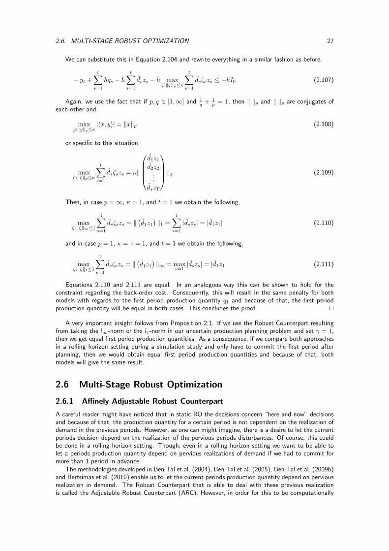
Albeit the l∞-norm and l1-norm being the complete opposite of each other, they show some resemblancefor certain input parameters. This is especially true when simulating the models in a rolling horizonfashion where only the next period’s production quantity has to be committed after planning.
In Proposition 2.1 we show that for certain input parameters the first period production quantities,q1 are equal in case a l∞-norm or l1-norms is used.
Proposition 2.1. Consider the semi-infinite optimization problem found in Problem 2.3. No matterwhich of the two uncertainty sets, U∞ or U1, we are using, if γ = 1 and the demand half-length forperiod t is equal in both Robust Counterparts, then the resulting first period production quantities fromboth models are equal.
Proof. For an arbitrary uncertainty set Up, p = 1 ∨ p =∞, and time period t, consider the constraintrelated to holding inventory,
− yt +
t∑s=1
hqs − ht∑
s=1
dszs ≤ −hI0 ∀d ∈ Up (2.104)
Remark that the demand vector is parameterized in an affine fashion by the perturbation vectors,
d(ζ) = d0 +
T∑t=1
dtζt ‖ζ‖p ≤ κ (2.105)
and that the per period demand can then be described as follows,
dt(ζ) = dt + dtζt |ζt| ≤ κ (2.106)
2.6. MULTI-STAGE ROBUST OPTIMIZATION 27
We can substitute this in Equation 2.104 and rewrite everything in a similar fashion as before,
− yt +
t∑s=1
hqs − ht∑
s=1
dszs − h maxζ:‖ζ‖p≤κ
t∑s=1
dsζszs ≤ −hI0 (2.107)
Again, we use the fact that if p, q ∈ [1,∞] and 1q + 1
p = 1, then ‖.‖p and ‖.‖p are conjugates ofeach other and,
maxy:‖y‖q≤κ
|〈x, y〉| = ‖x‖p (2.108)
or specific to this situation,
maxζ:‖ζ‖p≤κ
t∑s=1
dsζszs = κ‖
d1z1d2z2
...
dszT
‖q (2.109)
Then, in case p =∞, κ = 1, and t = 1 we obtain the following,
maxζ:‖ζ‖∞≤1
1∑s=1
dsζszs = ‖(d1z1
)‖1 =
1∑s=1
|dszs| = |d1z1| (2.110)
and in case p = 1, κ = γ = 1, and t = 1 we obtain the following,
maxζ:‖ζ‖1≤1
1∑s=1
dsζszs = ‖(d1z1
)‖∞ = max
s=1|dszs| = |d1z1| (2.111)
Equations 2.110 and 2.111 are equal. In an analogous way this can be shown to hold for theconstraint regarding the back-order cost. Consequently, this will result in the same penalty for bothmodels with regards to the first period production quantity q1 and because of that, the first periodproduction quantity will be equal in both cases. This concludes the proof.
A very important insight follows from Proposition 2.1. If we use the Robust Counterpart resultingfrom taking the l∞-norm or the l1-norm in our uncertain production planning problem and set γ = 1,then we get equal first period production quantities. As a consequence, if we compare both approachesin a rolling horizon setting during a simulation study and only have to commit the first period afterplanning, then we would obtain equal first period production quantities and because of that, bothmodels will give the same result.
2.6 Multi-Stage Robust Optimization
2.6.1 Affinely Adjustable Robust Counterpart
A careful reader might have noticed that in static RO the decisions concern “here and now” decisionsand because of that, the production quantity for a certain period is not dependent on the realization ofdemand in the previous periods. However, as one can might imagine, there is a desire to let the currentperiods decision depend on the realization of the pervious periods disturbances. Of course, this couldbe done in a rolling horizon setting. Though, even in a rolling horizon setting we want to be able tolet a periods production quantity depend on pervious realizations of demand if we had to commit formore than 1 period in advance.
The methodologies developed in Ben-Tal et al. (2004), Ben-Tal et al. (2005), Ben-Tal et al. (2009b)and Bertsimas et al. (2010) enable us to let the current periods production quantity depend on perviousrealization in demand. The Robust Counterpart that is able to deal with these previous realizationis called the Adjustable Robust Counterpart (ARC). However, in order for this to be computationally
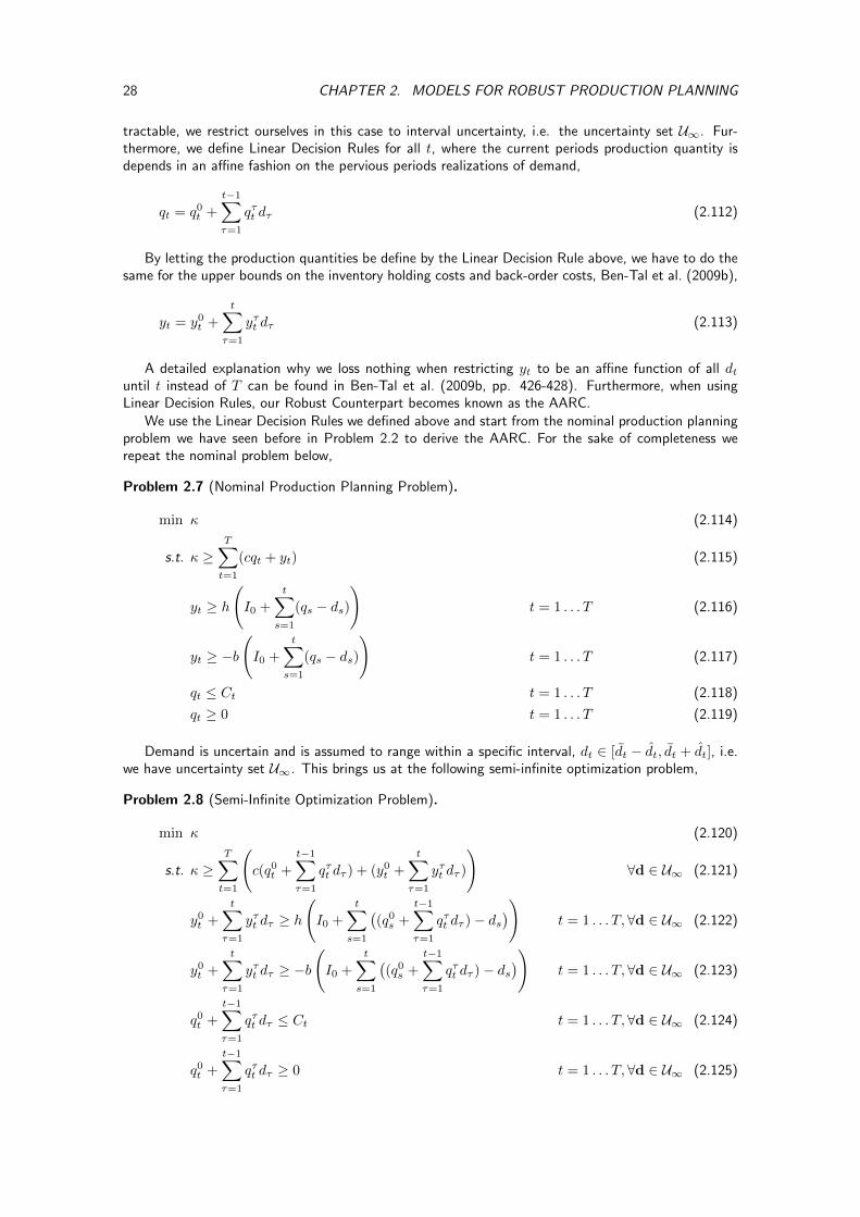
28 CHAPTER 2. MODELS FOR ROBUST PRODUCTION PLANNING
tractable, we restrict ourselves in this case to interval uncertainty, i.e. the uncertainty set U∞. Fur-thermore, we define Linear Decision Rules for all t, where the current periods production quantity isdepends in an affine fashion on the pervious periods realizations of demand,
qt = q0t +
t−1∑τ=1
qτt dτ (2.112)
By letting the production quantities be define by the Linear Decision Rule above, we have to do thesame for the upper bounds on the inventory holding costs and back-order costs, Ben-Tal et al. (2009b),
yt = y0t +
t∑τ=1
yτt dτ (2.113)
A detailed explanation why we loss nothing when restricting yt to be an affine function of all dtuntil t instead of T can be found in Ben-Tal et al. (2009b, pp. 426-428). Furthermore, when usingLinear Decision Rules, our Robust Counterpart becomes known as the AARC.
We use the Linear Decision Rules we defined above and start from the nominal production planningproblem we have seen before in Problem 2.2 to derive the AARC. For the sake of completeness werepeat the nominal problem below,
Problem 2.7 (Nominal Production Planning Problem).
min κ (2.114)
s.t. κ ≥T∑t=1
(cqt + yt) (2.115)
yt ≥ h
(I0 +
t∑s=1
(qs − ds)
)t = 1 . . . T (2.116)
yt ≥ −b
(I0 +
t∑s=1
(qs − ds)
)t = 1 . . . T (2.117)
qt ≤ Ct t = 1 . . . T (2.118)
qt ≥ 0 t = 1 . . . T (2.119)
Demand is uncertain and is assumed to range within a specific interval, dt ∈ [dt − dt, dt + dt], i.e.we have uncertainty set U∞. This brings us at the following semi-infinite optimization problem,
Problem 2.8 (Semi-Infinite Optimization Problem).
min κ (2.120)
s.t. κ ≥T∑t=1
(c(q0t +
t−1∑τ=1
qτt dτ ) + (y0t +
t∑τ=1
yτt dτ )
)∀d ∈ U∞ (2.121)
y0t +
t∑τ=1
yτt dτ ≥ h
(I0 +
t∑s=1
((q0s +
t−1∑τ=1
qτt dτ )− ds))
t = 1 . . . T, ∀d ∈ U∞ (2.122)
y0t +
t∑τ=1
yτt dτ ≥ −b
(I0 +
t∑s=1
((q0s +
t−1∑τ=1
qτt dτ )− ds))
t = 1 . . . T, ∀d ∈ U∞ (2.123)
q0t +
t−1∑τ=1
qτt dτ ≤ Ct t = 1 . . . T, ∀d ∈ U∞ (2.124)
q0t +
t−1∑τ=1
qτt dτ ≥ 0 t = 1 . . . T, ∀d ∈ U∞ (2.125)
2.6. MULTI-STAGE ROBUST OPTIMIZATION 29
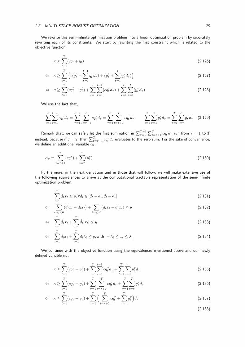
We rewrite this semi-infinite optimization problem into a linear optimization problem by separatelyrewriting each of its constraints. We start by rewriting the first constraint which is related to theobjective function,
κ ≥T∑t=1
(cqt + yt) (2.126)
⇔ κ ≥T∑t=1
(c(q0t +
t−1∑τ=1
qτt dτ ) + (y0t +
t∑τ=1
yτt dτ ))
(2.127)
⇔ κ ≥T∑t=1
(cq0t + y0t ) +
T∑t=1
t−1∑τ=1
(cqτt dτ ) +
T∑t=1
t∑τ=1
(yτt dτ ) (2.128)
We use the fact that,
T∑t=1
t−1∑τ=1
cqτt dτ =
T−1∑τ=1
T∑t=τ+1
cqτt dτ =
T∑τ=1
T∑t=τ+1
cqτt dτ ,
T∑t=1
t∑τ=1
yτt dτ =
T∑τ=1
T∑t=τ
yτt dτ (2.129)
Remark that, we can safely let the first summation in∑T−1τ=1
∑Tt=τ+1 cq
τt dτ run from τ = 1 to T
instead, because if τ = T then∑Tt=τ+1 cq
τt dτ evaluates to the zero sum. For the sake of convenience,
we define an additional variable αt,
ατ ≡T∑
t=τ+1
(cqτt ) +
T∑t=τ
(yτt ) (2.130)
Furthermore, in the next derivation and in those that will follow, we will make extensive use ofthe following equivalences to arrive at the computational tractable representation of the semi-infiniteoptimization problem.
T∑t=1
dtxt ≤ y,∀dt ∈ [dt − dt, dt + dt] (2.131)
⇔∑t:xt<0
(dtxt − dtxt) +∑t:xt>0
(dtxt + dtxt) ≤ y (2.132)
⇔T∑t=1
dtxt +
T∑t=1
dt|xt| ≤ y (2.133)
⇔T∑t=1
dtxt +
T∑t=1
dtλt ≤ y,with − λt ≤ xt ≤ λt (2.134)
We continue with the objective function using the equivalences mentioned above and our newlydefined variable ατ .
κ ≥T∑t=1
(cq0t + y0t ) +
T∑t=1
t−1∑τ=1
cqτt dτ +
T∑t=1
t∑τ=1
yτt dτ (2.135)
⇔ κ ≥T∑t=1
(cq0t + y0t ) +
T∑τ=1
T∑t=τ+1
cqτt dτ +
T∑τ=1
T∑t=τ
yτt dτ (2.136)
⇔ κ ≥T∑t=1
(cq0t + y0t ) +
T∑τ=1
( T∑t=τ+1
cqτt +
T∑t=τ
yτt
)dτ (2.137)
(2.138)
30 CHAPTER 2. MODELS FOR ROBUST PRODUCTION PLANNING
⇔ κ ≥T∑t=1
(cq0t + y0t ) +
T∑τ=1
ατdτ (2.139)
⇔ κ ≥T∑t=1
(cq0t + y0t ) +
T∑τ=1
ατ dτ +
T∑τ=1
|ατ |dτ (2.140)
⇔ κ ≥T∑t=1
(cq0t + y0t ) +
T∑τ=1
ατ dτ +
T∑τ=1
λτ dτ (2.141)
with −λτ ≤ ατ ≤ λτ . In a similar fashion we continue by rewriting the constraint related to theinventory balance equation, starting with the part related to the inventory holding costs.
yt ≥ h
(I0 +
t∑s=1
(qs − ds)
)(2.142)
⇔ yt ≥ hI0 + h
t∑s=1
qs − ht∑
s=1
ds (2.143)
⇔ y0t +
t∑τ=1
yτt dτ ≥ hI0 + h
t∑s=1
(q0s +
s−1∑τ=1
qτs dτ )− ht∑
s=1
ds (2.144)
⇔ y0t +
t∑τ=1
yτt dτ ≥ hI0 + h
t∑s=1
q0s + h
t∑s=1
s−1∑τ=1
qτs dτ − ht∑
s=1
ds (2.145)
⇔ y0t +
t∑τ=1
yτt dτ ≥ hI0 + h
t∑s=1
q0s + h
t−1∑τ=1
t∑s=τ+1
qτs dτ − ht∑
τ=1
dτ (2.146)
⇔ − hI0 ≥ ht∑
s=1
q0s − y0t −t∑
τ=1
yτt dτ + h
t−1∑τ=1
t∑s=τ+1
qτs dτ − ht∑
τ=1
dτ (2.147)
Again, remark that in case τ = t, then the summation∑ts=τ+1 q
τs evaluates to the zero sum.
Therefore, we can extend the range of the summation in a similar way as before. Furthermore, wedefine additional variable γτt ,
γτt ≡ yτt − ht∑
s=τ+1
qτs + h (2.148)
and use this to obtain,
∀t, − hI0 ≥ ht∑
s=1
q0s − y0t −t∑
τ=1
((yτt − h
t∑s=τ+1
qτs + h)dτ)
(2.149)
⇔ − hI0 ≥ ht∑
s=1
q0s − y0t −t∑
τ=1
γτt dτ (2.150)
⇔ − hI0 ≥ ht∑
s=1
q0s − y0t −t∑
τ=1
γτt dτ +
t∑τ=1
|γτt |dτ (2.151)
⇔ − hI0 ≥ ht∑
s=1
q0s − y0t −t∑
τ=1
γτt dτ +
t∑τ=1
πτt dτ (2.152)
with −πτt ≤ γτt ≤ πτt . Analogous to the constraint related to the inventory holding costs we rewrite
2.6. MULTI-STAGE ROBUST OPTIMIZATION 31
the part related to the back-order costs.
∀t, yt ≥ −b
(I0 +
t∑s=1
(qs − ds)
)(2.153)
⇔ yt ≥ −bI0 − bt∑
s=1
qs + b
t∑s=1
ds (2.154)
⇔ y0t +
t∑τ=1
yτt dτ ≥ −bI0 − bt∑
s=1
(q0s +
s−1∑τ=1
qτs dτ ) + b
t∑s=1
ds (2.155)
⇔ y0t +
t∑τ=1
yτt dτ ≥ −bI0 − bt∑
s=1
q0s − bt∑
s=1
s−1∑τ=1
qτs dτ + b
t∑s=1
ds (2.156)
⇔ y0t +
t∑τ=1
yτt dτ ≥ −bI0 − bt∑
s=1
q0s − bt−1∑τ=1
t∑s=τ+1
qτs dτ + b
t∑τ=1
dτ (2.157)
⇔ bI0 ≥ −bt∑
s=1
q0s − y0t −t∑
τ=1
yτt dτ − bt−1∑τ=1
t∑s=τ+1
qτs dτ + b
t∑τ=1
dτ (2.158)
We define additional variable ωτt ,
ωτt ≡ yτt + b
t∑s=τ+1
qτs − b (2.159)
and use this to obtain,
∀t, bI0 ≥ −bt∑
s=1
q0s − y0t −t∑
τ=1
((yτt + b
t∑s=τ+1
qτs − b)dτ)
(2.160)
⇔ bI0 ≥ −bt∑
s=1
q0s − y0t −t∑
τ=1
ωτt dτ (2.161)
⇔ bI0 ≥ −bt∑
s=1
q0s − y0t −t∑
τ=1
ωτt dτ +
t∑τ=1
|ωτt |dτ (2.162)
⇔ bI0 ≥ −bt∑
s=1
q0s − y0t −t∑
τ=1
ωτt dτ +
t∑τ=1
φτt dτ (2.163)
with −φτt ≤ ωτt ≤ φτt . Next is the capacity related constraint, it readily follows from using theequivalences that,
qt ≤ Ct (2.164)
⇔ q0t +
t−1∑τ=1
qτt dτ ≤ Ct (2.165)
⇔ q0t +
t−1∑τ=1
qτt dτ +
t−1∑τ=1
|qτt |dτ ≤ Ct (2.166)
⇔ q0t +
t−1∑τ=1
qτt dτ +
t−1∑τ=1
ψτt dτ ≤ Ct (2.167)
32 CHAPTER 2. MODELS FOR ROBUST PRODUCTION PLANNING
with, −ψτt ≤ qτt ≤ ψτt . Likewise for the lower bound on qt,
∀t, qt ≥ 0 (2.168)
⇔ q0t +
t−1∑τ=1
qτt dτ ≥ 0 (2.169)
⇔ q0t +
t−1∑τ=1
qτt dτ +
t−1∑τ=1
|qτt |dτ ≥ 0 (2.170)
⇔ q0t +
t−1∑τ=1
qτt dτ +
t−1∑τ=1
ψτt dτ ≥ 0 (2.171)
with, −ψτt ≤ qτt ≤ ψτt . Finally, we are able to combine each of the constraints that we haverewritten, to obtain the the AARC of the Semi-Infinite Optimization that we started with.
Problem 2.9 (Affinely Adjustable Robust Counterpart for U∞).
min κ (2.172)
s.t. κ ≥T∑t=1
(cq0t + y0t ) +
T∑τ=1
ατ dτ +
T∑τ=1
λτ dτ (2.173)
ατ =
T∑t=τ+1
(cqτt ) +
T∑t=τ
(yτt ) τ = 1 . . . T (2.174)
− λτ ≤ ατ ≤ λτ τ = 1 . . . T (2.175)
− hI0 ≥ ht∑
s=1
q0s − y0t −t∑
τ=1
γτt dτ +
t∑τ=1
πτt dτ t = 1 . . . T (2.176)
bI0 ≥ −bt∑
s=1
q0s − y0t −t∑
τ=1
ωτt dτ +
t∑τ=1
φτt dτ t = 1 . . . T (2.177)
γτt = yτt − ht∑
s=τ+1
qτs + h τ = 1 . . . T, t = 1 . . . T (2.178)
ωτt = yτt + b
t∑s=τ+1
qτs − b τ = 1 . . . T, t = 1 . . . T (2.179)
− πτt ≤ γτt ≤ πτt τ = 1 . . . T, t = 1 . . . T (2.180)
− φτt ≤ ωτt ≤ φτt τ = 1 . . . T, t = 1 . . . T (2.181)
q0t +
t−1∑τ=1
qτt dτ +
t−1∑τ=1
ψτt dτ ≤ Ct t = 1 . . . T (2.182)
q0t +
t−1∑τ=1
qτt dτ +
t−1∑τ=1
ψτt dτ ≥ 0 t = 1 . . . T (2.183)
− ψτt ≤ qτt ≤ ψτt t = 1 . . . T, τ < t (2.184)
where κ, {qτt }, {yτt }, {ατ}, {λτ}, {γτt }, {πτt }, {ωτt }, {φτt } and {ψτt } are the decision variables thattogether make up the decision vector.
2.6.2 Adjustable Robust Mixed-Integer Optimization
So far we have discussed the techniques and methodologies of RO based on a basic production planningproblem. These techniques and methodologies form the state of the art. Though, as in most fields,things will continue to evolve and this will lead to new opportunities. This is also the case for AdjustableRO in case of integer (or binary) decision variables. It must be mentioned that the AARC will not work
2.7. DISTRIBUTIONALLY ROBUST OPTIMIZATION 33
in case of integer (or binary) decision variables, because this would mean that the integer (or binary)decision variable has be expressed as a Linear Decision Rule and this is clearly not possible. This makesit impossible to use this technique in the next chapter, because we will work with a binary decisionvariable there to decide on production setups.
However, it is worth mentioning that work has been done to deal with integer (or binary) decisionvariables in Adjustable RO, but according to Bertsimas and Georghiou (2015) the results are far fromoptimal. Though, at the time of writing two articles came into being that seem to be promising insolving this issue, but they emerged to late to incorporate in this work. Nevertheless, the interestedreader is recommended to look at the work of Bertsimas and Georghiou (2015) or Postek and denHertog (2015)).
2.7 Distributionally Robust Optimization
We concluded the last section with some kind of a future outlook with regards to Adjustable RO.Besides that development, there is another one worth mentioning, namely Distributionally RO (DRO).
We started in this chapter with a generic representation of multi-stage decision problems. This ledto our nominal production planning problem and eventually, we introduced uncertainty in it. We didso in a more or less geometrical way, so to say, because we extended the normal polyhedron to whicha optimal solution should belong, e.g. by using interval uncertainty. However, there is a significantpart of research that deals with uncertainty by means of a probability distribution, i.e. the techniquesaround Stochastic Programming. So traditionally, there are two ways to deal with uncertainty, i.e. ina geometrical way as RO does or in a stochastic way as in Stochastic Programming.
However, quite recently, DRO gained widespread attention and can be regarded as a third method.This method appears to be closing the gap between the two fields, because it borrows the probabilisticnotion of uncertainty from the stochastic world and combines it with the ability to come up with tractableresults from RO. The latter is something Stochastic Programming suffers from for large instances andthis issue is known as the curse of dimensionality.
We have discussed before that in case of RO we want our constraints to hold for each possiblerealization of the parameters z belonging to uncertainty set U ,
supz∈U
f(x, z) ≤ 0 (2.185)
Though, in case of Stochastic Programming, parameter z would be a random variable belonging toa known probability distribution and we start solving the problem from there. However, it is not strictlythe case that this probability distribution is known, or known with certainty. DRO takes a differentapproach in this. It still assumes parameter z to be a random variable, but the probability distribution isunknown. The only information known are the first few moments, e.g. the mean, variance and perhapsskewness. The random parameter z has a distribution Pz and belongs to the so called ambiguity set P.In this setting there are two constraints one can distinct: the worst-case expected feasibility constraint,
supPz∈P
EPz[f(x, z)] ≤ 0 (2.186)
and chance constraints,
supPz∈P
P [f(x, z)] ≤ ε (2.187)
The literature of this type of problem started with the work of Scarf et al. (1958), but meanwhile itgained more and more attention and quite recently a paper by Postek et al. (2015) puts it back on themap. With most work still being of aimed at developing methodologies, the techniques of DRO are inits infancy, but they are worth to keep an eye on in the future.
2.8 Conclusion
In this chapter we started with a generic multi-stage decision problem and showed that a simple produc-tion planning problem can be represented as such. This problem took the form of a Linear Optimization
34 CHAPTER 2. MODELS FOR ROBUST PRODUCTION PLANNING
problem. We have introduced demand uncertainty herein in a geometrical way. For various types ofuncertainty sets we have shown how to come up with its Robust Counterpart. We have even seen one,the one with cardinality constraint uncertainty, where the uncertainty can be controlled per period bymeans of a parameter. Thereafter, we made the extension to the Affinely Adjustable Robust Counter-part. This enabled us to take into consideration the pervious realizations of demand if we are planningfor the next period. Furthermore, we have discussed some interesting properties with regards of theoptimality and we concluded this chapter with a future outlook on RO. The outlook is mend to bemore of a reminder of the potential of RO. With the knowledge gained in this chapter, we will be ableto apply its techniques and methodologies to a more complicated production planning problem whichforms the core of this thesis: the CLSP. For sure, we can answer confirmative to the first of our researchquestions: yes, we can apply the methodologies of RO to production planning problems.
Chapter 3
The Capacitated Lot-Sizing Problemunder Demand Uncertainty
3.1 Introduction
In this chapter we study the CLSP in case of deterministic demand and in case of uncertain demand.We start in the next section with formulating the problem as a Mixed Integer LO problem in caseof dynamic and time-varying demand. Despite the computational challenges that come with such aformulation, we do stick with it as it provides nice grounds for introducing a stochastic as well as arobust counterpart. In the next chapter we discuss the simulation study in which these models will besubject to thorough testing and analysis.
3.2 The Deterministic Capacitated Lot Sizing Problems
3.2.1 The Problem
The CLSP discussed in this chapter is a finite-horizon, periodic review, multi-item, single locationproduction planning problem. Basically, we extend the single item production planning situation of theprevious chapter, into one where we have to plan production for multiple items on one machine withlimited capacity, while incurring setup and holding costs. The presence of inventory holding costs andsetup costs leads to the trade-off between holding more inventory or switching between producing acertain item more often. Of course, all while taking into account the per period capacity restrictions.The capacity restriction in case of deterministic demand makes the CLSP an extension of the well-knowndynamic lot sizing problem by Wagner and Whitin (1958).
In our case it is allowed to produce different types of products in one period. Hence, the CLSP is ofa “big bucket” type of problem (Helber et al. (2013)). Contrary to “small-bucket” problems where theperiods are set smaller and we have to decide how much periods to produce a certain product beforeswitching to producing another product in a later period.
Capacity is expressed as the amount of time units available for production and setting up production.Capacity is then only consumed by the time required to setup the machine before production cancommence and capacity is consumed by the time needed to produce the items of that time period.
As has been mentioned before, we first assume demand to be deterministic and that the availablecapacity is sufficiently large to satisfy demand. However, when capacity becomes a scares resource andwhen demand becomes stochastic, we might run into trouble. The reason for this is that we mightneed more capacity than available due to an extreme realization of demand to satisfy our service levelconstraint. Therefore, we relax the model in order to overcome this problem and to ensure that westill end up with a feasible production plan. We do so by introducing overtime, which evidently comesat a certain cost. The price of overtime is set in such a way that it is undesirable to use it, becausethis would result in the most fair way to study the trade of between holding inventory and setting upproduction. Note, that the aim is to come up with a feasible production plan, not really to have extracapacity.
35
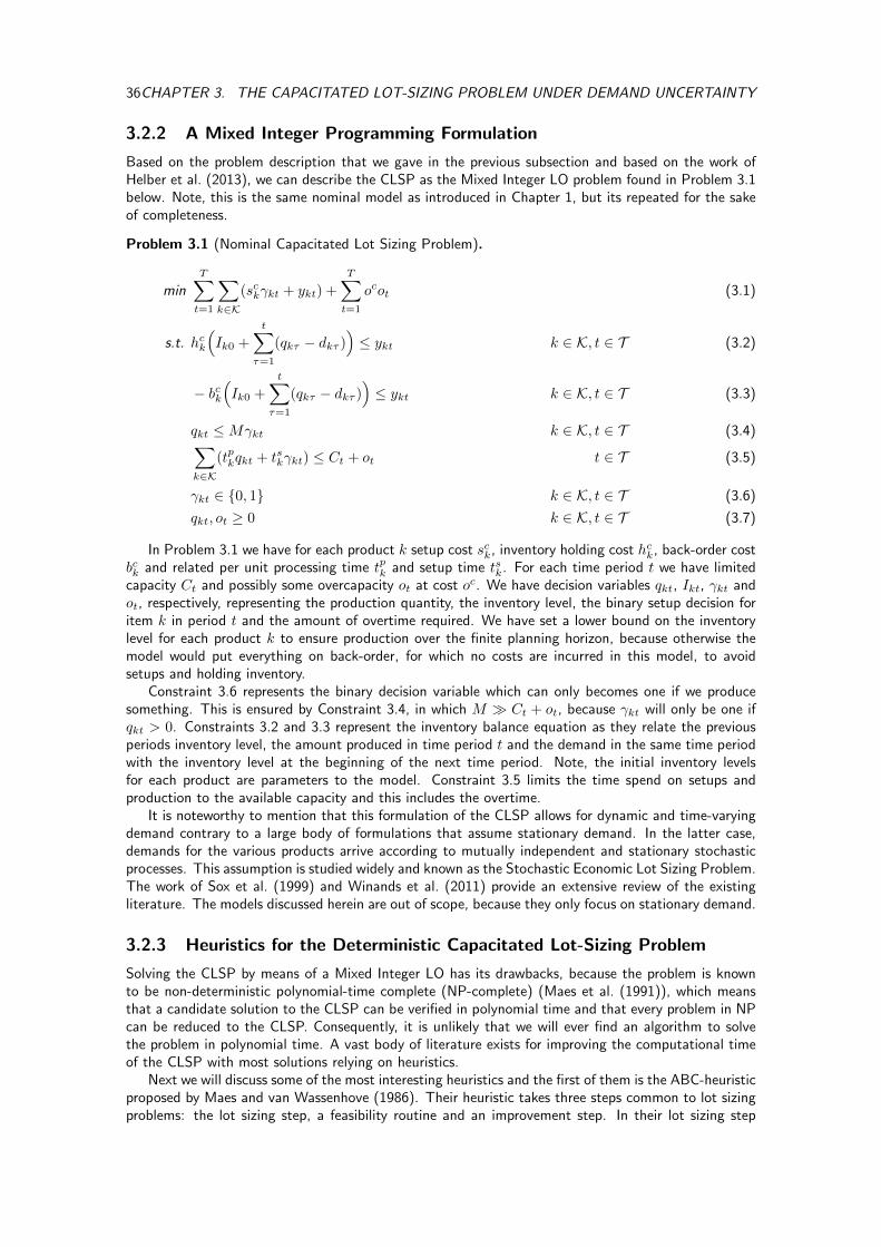
36CHAPTER 3. THE CAPACITATED LOT-SIZING PROBLEM UNDER DEMAND UNCERTAINTY
3.2.2 A Mixed Integer Programming Formulation
Based on the problem description that we gave in the previous subsection and based on the work ofHelber et al. (2013), we can describe the CLSP as the Mixed Integer LO problem found in Problem 3.1below. Note, this is the same nominal model as introduced in Chapter 1, but its repeated for the sakeof completeness.
Problem 3.1 (Nominal Capacitated Lot Sizing Problem).
minT∑t=1
∑k∈K
(sckγkt + ykt) +
T∑t=1
ocot (3.1)
s.t. hck
(Ik0 +
t∑τ=1
(qkτ − dkτ ))≤ ykt k ∈ K, t ∈ T (3.2)
− bck(Ik0 +
t∑τ=1
(qkτ − dkτ ))≤ ykt k ∈ K, t ∈ T (3.3)
qkt ≤Mγkt k ∈ K, t ∈ T (3.4)∑k∈K
(tpkqkt + tskγkt) ≤ Ct + ot t ∈ T (3.5)
γkt ∈ {0, 1} k ∈ K, t ∈ T (3.6)
qkt, ot ≥ 0 k ∈ K, t ∈ T (3.7)
In Problem 3.1 we have for each product k setup cost sck, inventory holding cost hck, back-order costbck and related per unit processing time tpk and setup time tsk. For each time period t we have limitedcapacity Ct and possibly some overcapacity ot at cost oc. We have decision variables qkt, Ikt, γkt andot, respectively, representing the production quantity, the inventory level, the binary setup decision foritem k in period t and the amount of overtime required. We have set a lower bound on the inventorylevel for each product k to ensure production over the finite planning horizon, because otherwise themodel would put everything on back-order, for which no costs are incurred in this model, to avoidsetups and holding inventory.
Constraint 3.6 represents the binary decision variable which can only becomes one if we producesomething. This is ensured by Constraint 3.4, in which M � Ct + ot, because γkt will only be one ifqkt > 0. Constraints 3.2 and 3.3 represent the inventory balance equation as they relate the previousperiods inventory level, the amount produced in time period t and the demand in the same time periodwith the inventory level at the beginning of the next time period. Note, the initial inventory levelsfor each product are parameters to the model. Constraint 3.5 limits the time spend on setups andproduction to the available capacity and this includes the overtime.
It is noteworthy to mention that this formulation of the CLSP allows for dynamic and time-varyingdemand contrary to a large body of formulations that assume stationary demand. In the latter case,demands for the various products arrive according to mutually independent and stationary stochasticprocesses. This assumption is studied widely and known as the Stochastic Economic Lot Sizing Problem.The work of Sox et al. (1999) and Winands et al. (2011) provide an extensive review of the existingliterature. The models discussed herein are out of scope, because they only focus on stationary demand.
3.2.3 Heuristics for the Deterministic Capacitated Lot-Sizing Problem
Solving the CLSP by means of a Mixed Integer LO has its drawbacks, because the problem is knownto be non-deterministic polynomial-time complete (NP-complete) (Maes et al. (1991)), which meansthat a candidate solution to the CLSP can be verified in polynomial time and that every problem in NPcan be reduced to the CLSP. Consequently, it is unlikely that we will ever find an algorithm to solvethe problem in polynomial time. A vast body of literature exists for improving the computational timeof the CLSP with most solutions relying on heuristics.
Next we will discuss some of the most interesting heuristics and the first of them is the ABC-heuristicproposed by Maes and van Wassenhove (1986). Their heuristic takes three steps common to lot sizingproblems: the lot sizing step, a feasibility routine and an improvement step. In their lot sizing step
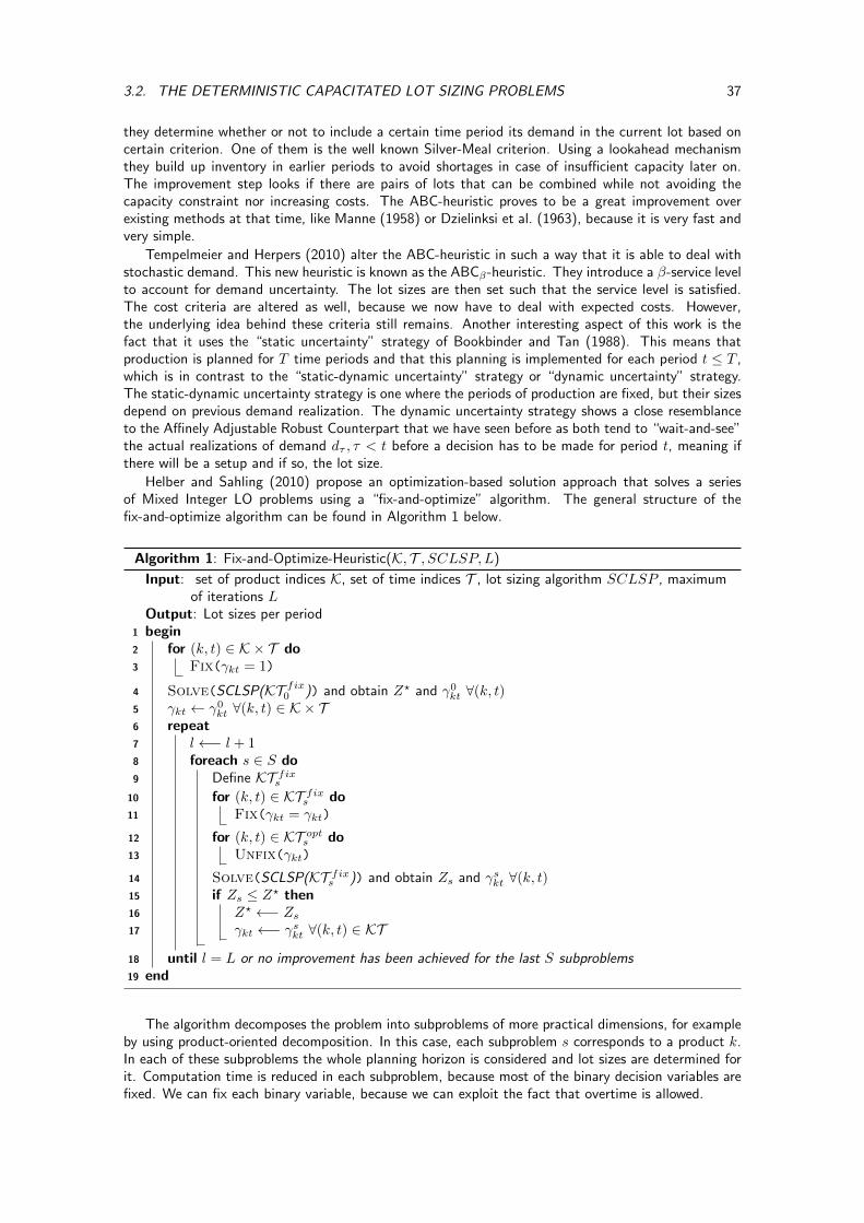
3.2. THE DETERMINISTIC CAPACITATED LOT SIZING PROBLEMS 37
they determine whether or not to include a certain time period its demand in the current lot based oncertain criterion. One of them is the well known Silver-Meal criterion. Using a lookahead mechanismthey build up inventory in earlier periods to avoid shortages in case of insufficient capacity later on.The improvement step looks if there are pairs of lots that can be combined while not avoiding thecapacity constraint nor increasing costs. The ABC-heuristic proves to be a great improvement overexisting methods at that time, like Manne (1958) or Dzielinksi et al. (1963), because it is very fast andvery simple.
Tempelmeier and Herpers (2010) alter the ABC-heuristic in such a way that it is able to deal withstochastic demand. This new heuristic is known as the ABCβ-heuristic. They introduce a β-service levelto account for demand uncertainty. The lot sizes are then set such that the service level is satisfied.The cost criteria are altered as well, because we now have to deal with expected costs. However,the underlying idea behind these criteria still remains. Another interesting aspect of this work is thefact that it uses the “static uncertainty” strategy of Bookbinder and Tan (1988). This means thatproduction is planned for T time periods and that this planning is implemented for each period t ≤ T ,which is in contrast to the “static-dynamic uncertainty” strategy or “dynamic uncertainty” strategy.The static-dynamic uncertainty strategy is one where the periods of production are fixed, but their sizesdepend on previous demand realization. The dynamic uncertainty strategy shows a close resemblanceto the Affinely Adjustable Robust Counterpart that we have seen before as both tend to “wait-and-see”the actual realizations of demand dτ , τ < t before a decision has to be made for period t, meaning ifthere will be a setup and if so, the lot size.
Helber and Sahling (2010) propose an optimization-based solution approach that solves a seriesof Mixed Integer LO problems using a “fix-and-optimize” algorithm. The general structure of thefix-and-optimize algorithm can be found in Algorithm 1 below.
Algorithm 1: Fix-and-Optimize-Heuristic(K, T , SCLSP,L)
Input: set of product indices K, set of time indices T , lot sizing algorithm SCLSP , maximumof iterations L
Output: Lot sizes per periodbegin1
for (k, t) ∈ K × T do2
Fix(γkt = 1)3
Solve(SCLSP(KT fix0 )) and obtain Z? and γ0kt ∀(k, t)4
γkt ← γ0kt ∀(k, t) ∈ K × T5
repeat6
l←− l + 17
foreach s ∈ S do8
Define KT fixs9
for (k, t) ∈ KT fixs do10
Fix(γkt = γkt)11
for (k, t) ∈ KT opts do12
Unfix(γkt)13
Solve(SCLSP(KT fixs )) and obtain Zs and γskt ∀(k, t)14
if Zs ≤ Z? then15
Z? ←− Zs16
γkt ←− γskt ∀(k, t) ∈ KT17
until l = L or no improvement has been achieved for the last S subproblems18
end19
The algorithm decomposes the problem into subproblems of more practical dimensions, for exampleby using product-oriented decomposition. In this case, each subproblem s corresponds to a product k.In each of these subproblems the whole planning horizon is considered and lot sizes are determined forit. Computation time is reduced in each subproblem, because most of the binary decision variables arefixed. We can fix each binary variable, because we can exploit the fact that overtime is allowed.
38CHAPTER 3. THE CAPACITATED LOT-SIZING PROBLEM UNDER DEMAND UNCERTAINTY
For the remainder of this chapter as well as for the remainder of this thesis, we will leave theheuristics mentioned above out of consideration. We will only focus on comparing methods purelybased on mathematical optimization, because these are the ones that lend themselves very well for aRobust Optimization approach. Nevertheless, it should be mentioned that in future research, some ofthese heuristics, like the fix-and-optimize algorithm, might be used to improve the computation time.
3.3 The Stochastic Capacitated Lot Sizing Problem
3.3.1 The Introduction of Demand Uncertainty
In the previous section we looked at methods to solve the CLSP when the per period demand wasknown at the beginning of the planning horizon. In this section we only consider the case wheredemand is uncertain. More specifically, first we let the per period demands be random variables of aknown probability distribution, the Normal distribution. From the work of Helber et al. (2013), Rossiet al. (2015) and Tempelmeier and Hilger (2015) it becomes clear that literature is dominated by theuse of the Normal distribution. That is why we will use this distribution in our model too. However,it must be noted that the methods and techniques found in this section can be made specific to otherprobability distributions as well. After considering stochastic models that deal with demand uncertainty,we continue with a Robust Optimization approach to the problem.
With the introduction of uncertainty by means of random variables, we arrive at the stochasticcounterpart of the CLSP. For each product k the per period demands are independently and identicallydistributed with dkt ∼ Normal(µdk , σdk). For each product k in each time period t we have, probabilitydensity function fdkt
, cumulative density function Fdkt, forecasted expected value E[dkt] = µdk and
variance V ar[dkt] = σ2dkt
. From now on we no longer talk about demand, back-orders or inventorylevel, but we have to work with their expected values. Therefore, we have to rewrite the nominal CLSPfound in Problem 3.1 to account for the stochastic nature of the per period demand.
First, we take a look at the inventory level Ikt variable that occurs in the objective function andthe inventory balance equation. The expected inventory level for product k is determined based onthe cumulative demand Dkt and cumulative production quantity Qkt up to period t. The cumulativedemand Dkt equals the sum of t independent and identically normally distributed random variables.
Hence, cumulative demand is Normal, Dkt ∼ Normal(µDk=∑tτ=1 µdk , σDk
=√∑t
τ=1 σ2dk
) with
fDktand FDkt
, respectively, being the probability density function and cumulative density function(Ross, 2010, pp. 67-68). Using these cumulative measures we can express the expected inventory levelas follows,
E[Ikt] = E[max{0, Qkt −Dkt}] =
∫ Qkt
0
(Qkt − x)fDkt(x)dx k ∈ K, t ∈ T (3.8)
Working with the cumulative measures combined with the fact that the inventory balance equationcan be written in a closed form, results in the following expression for the inventory level,
Ikt = Ik,t−1 + qkt − dkt k ∈ K, t ∈ T (3.9)
= Ik0 +
t∑τ=1
qkτ − dkτ k ∈ K, t ∈ T (3.10)
= Ik0 +Qkt −Dkt k ∈ K, t ∈ T (3.11)
This expression can be substituted in the objective function of the nominal CLSP such that we caneliminate the inventory balance equation. For now, we assume that the initial inventory level Ik0 equalszero. Later on, we will extend the model to work with an arbitrary initial inventory level unequal tozero.
Second, in the Stochastic CLSP we do allow back-orders and we have control over them by means ofthe β-service level constraint. This means that the back-order cost become obsolete. The use of a servicelevel constraint is rather important in general, because it enables us to control the production quantitywith respect to demand. We have an infinitely large tail of probable demand realizations, becausedemand is normally distributed. This means that if we want to be able to satisfy all possible realizations
3.3. THE STOCHASTIC CAPACITATED LOT SIZING PROBLEM 39
of demand, we would need to produce an infinite amount of items for each product. Evidently, thisis impossible due to physical as well as financial reasons. Hence, the need for a service level becomesclear, because it allows us to specify the fraction of demand we want to satisfy.
Analogous to the expected inventory level, we can express the expected backlog, also known as thefirst order loss function, as follows,
L1Dkt
(Qkt) = E[Blkt] k ∈ T , t ∈ T (3.12)
= E[max{0, Dkt −Qkt}] k ∈ T , t ∈ T (3.13)
=
∫ ∞Qkt
(x−Qkt)fDkt(x)dx k ∈ T , t ∈ T (3.14)
Note the difference between backlog and back-orders. Back-orders are determined periodically,whereas backlog is a measure for the the cumulative amount of back-orders. So, period t its expectedback-orders equals,
E[Bkt] = L1Dkt
(Qkt)− L1Dk,t−1
(Qkt) (3.15)
The most common service level constraints are the α- and β-service level. They are, respectively,expressed as the probability of no stock-out or the percentage of demand directly satisfied from stock.For this reason the latter is also known as the fill-rate constraints. Besides that, both service levels arealso known in literature as the P1 service level and the P2 service level (see Silver et al. (1998)). Theinterested reader might consult the work of Helber and Sahling (2010) to get to known more aboutother service levels.
When combining all of the above and using an arbitrary service level constraint, we can formulatethe Stochastic CLSP found in Problem 3.2.
Problem 3.2 (Stochastic Capacitated Lot Sizing Problem).
minT∑t=1
∑k∈K
(sckγkt + hckE[Ikt]) +
T∑t=1
ocot (3.16)
s.t. qkt ≤Mγkt k ∈ K, t ∈ T (3.17)∑k∈K
tpkqkt + tskγkt ≤ Ct + ot t ∈ T (3.18)
service level constraint, to be specified (3.19)
γkt ∈ {0, 1} k ∈ K, t ∈ T (3.20)
qkt, ot ≥ 0 k ∈ K, t ∈ T (3.21)
In the remainder of this work we will stick to the β-service level for two reasons. First, according toTempelmeier and Hilger (2015) this is the one most used in practice and second, it is the one most widelyused in mathematical programming formulations for the SCLSP (see Tempelmeier (2007), Tempelmeierand Herpers (2010), Tempelmeier (2011) and Tempelmeier and Hilger (2015)). We mentioned beforethat the β-service level is the percentage of demand that should be directly satisfied from inventory.An exact definition is as follows,
1−∑Tt=1E[Bkt]∑Tt=1 dkt
≥ β k ∈ K (3.22)
If we want to work with the β-service level in the SCLSP found in Problem 3.2, then we replaceConstraint 3.19 with Equation 3.22.
Tempelmeier and Hilger (2015) however, define another service level constraint as well, i.e. theβc-service level. This service level ensures that the service level is achieved per cycle, because it relates
40CHAPTER 3. THE CAPACITATED LOT-SIZING PROBLEM UNDER DEMAND UNCERTAINTY
back-orders and demand during the cycle. They define it as follows,∑ti=1E[Bki]∑ti=1E[dki]
≥ 1− βc − (1− γk,t+1) k ∈ K, t ∈ T (3.23)∑ti=1E[Bki]∑ti=1E[dki]
≤ 1− βc + (1− γk,t+1) k ∈ K, t ∈ T (3.24)
γk,T+1 = 1 k ∈ K (3.25)
A careful reader might already have noticed that the use of the expected inventory level and expectedbacklog make the problem no longer a Linear Optimization problem, because their respective functionsare non-linear in the cumulative production quantity. We will continue in the next section with anexplicit derivation for both the expected inventory level and the expected backlog. These explicitderivations will be used to linearize both functions. Using the linearized versions of these function wewill be able to formulate the problem again as a Linear Optimization problem.
3.3.2 An Explicit Derivation for the Expected Backlog and Inventory Level
We start out with an explicit derivation for the expected backlog function. The backlog for product kdepends on the cumulative demand Dkt and cumulative quantity produced Qkt up to period t to fulfildemand. The backlog for product k in period k can be defined as follows,
Blkt(Qkt) =
{0 if Dkt ≤ QktDkt −Qkt if Dkt > Qkt
(3.26)
Using the definition above we can start our derivation, for any product k ∈ K and period t ∈ T ,
L1Dkt
(Qkt) = E[Blkt(Qkt)] (3.27)
= E[max{0, Dkt −Qkt}] (3.28)
=
∫ ∞−∞
max{0, x−Qkt}fDkt(x)dx (3.29)
=
∫ ∞Qkt
(x−Qkt)fDkt(x)dx (3.30)
The next step in the derivation relies on the fact that the PDF f(.) of the Normal distribution can be
written in terms of the standard Normal PDF, f(x) = 1σφ(x−µσ ). Furthermore, we define z =
Qkt−µDk
σDk.
L1Dkt
(Qkt) =
∫ ∞Qkt
(Dkt −Qkt)1
σDk
φ(x− µDk
σx
)dx (3.31)
= σDk
∫ ∞Qkt
((x− µDk
σDk
)− z) 1
σDk
φ(x− µDk
σDk
)dx (3.32)
In the next steps we, respectively, use the substitution rule for integration as expressed in EquationB.6 and integration by parts which is expressed in Equation B.7. Both rules for integration can befound in Appendix B.
{Using Equation B.6, substitution rule for integration }
L1Dkt
(Qkt) = σDk
∫ ∞z
(t− z)φ(t)dt (3.33)
= σDk
(∫ ∞z
tφ(t)dt−∫ ∞z
zφ(t)dt)
(3.34)
{Using Equation B.7, integration by parts }
= σDk
([tΦ(t)−
∫ ∞z
Φ(t)dt]]∣∣∣∞t=z− z(1− Φ(z))
)(3.35)
3.3. THE STOCHASTIC CAPACITATED LOT SIZING PROBLEM 41
The best way to understand the step made in going from Equation 3.32 to Equation 3.33, is to lookat it the other way around. Then think of (t− z)φ(t) as being the function f(x) in the integration bysubstitution rule of Equation B.6. Besides that, remark that the first derivative of z is as follows,
d
dQktz =
d
dQkt
(Qkt − µDk
σDk
)=
1
σDk
(3.36)
To rewrite the integrand in the last equation we use the fact that the antiderivative of the standardNormal CDF equals,
∫Φ(t)dt = tΦ(t) + φ(t).
L1kt(Qkt) = σDk
([tΦ(t)−
[tΦ(t) + φ(t)
]]∣∣∣∞t=z− z(1− Φ(z))
)(3.37)
= σDk
([− φ(t)
]∣∣∣∞t=z− z(1− Φ(z))
)(3.38)
= σDk
((−φ(∞) + φ(z)
)− z(1− Φ(z))
)(3.39)
= σDk
(φ(z)− z(1− Φ(z))
)(3.40)
This concludes our explicit derivation for the expected backlog. In an analogous fashion we canderive the expected inventory level for any t ∈ T and k ∈ K. This results in,
E[Ikt(Qkt)] = Qkt −Dkt + L1Dkt
(Qkt) (3.41)
= σDk
(φ(z) + z(1− Φ(−z))
)z =
Qkt − µDk
σDk
(3.42)
Clearly, the functions for the expected backlog and the expected inventory level are non-linear andwe have to linearize both to work with them in the Problem 3.2. Therefore, we will continue in thenext section with a piecewise linear approximation of both functions.
3.3.3 Linearizing the Expected Backlog and Expected Inventory Level Func-tions
In this section we describe how to linearize the functions for the expected inventory level and the expectedbacklog. We can approximate both functions over the range [0, uLkt] with an arbitrary precision using asufficient number of L line segments (see Helber et al. (2013), Rossi et al. (2014), Tempelmeier andHilger (2015) and Rossi et al. (2015)). An illustration of how such linearized functions would look likefor L = 12, uLkt = 200, E[Dkt] = 100 and V ar[Dkt] = 30 is shown in Figure 3.1. The figure showsthat the expected backlog drops as we produce more, while the expected inventory increases. Since,we only allow a certain number of expected back-orders, we have to produce to ensure the expectedbacklog is in line with our service level constraint. This directly relates to an increase in the expectedinventory level. This increase is not only influenced by the service level constraint, but also by thetrade-off between holding inventory and setting up more frequently. Therefore, choosing the optimalcumulative production quantity Qkt depends on achieving the required service level at minimum costwhile respecting the capacity constraint.
We can approximate the expected backlog and inventory level as follows. First, we have to definethe relevant region and divide this range into L closed intervals with endpoints ulkt. Endpoint u0ktequals zero, because is is not necessarily the case that we have to produce and because of that, weshould allow for zero production. Of course, this is still under the assumption of zero initial inventory.Furthermore, endpoint uLkt should be sufficiently large to account for the extra production required bythe service level constraint and the trade-off between holding inventory and setting up production. Ingeneral it should account for the following: the cumulative production in the past Qk,t−1 =
∑t−1τ=1 dkτ ,
the current periods demand dkt and the minimum of the available capacity and the optimal amount toproduce in advance.
We should include future demand dkτ , τ > t, into the current production lot qkt, if some costcriterion tells us that the costs are lower if we include it, then if we were not to include it. For example,we could take the cost criterion of Wagner and Whitin (1958) and define the following cost function,
Kww(t, x) = (sk + hk
x∑τ=t
(τ − t)dkτ )/(x− t) (3.43)
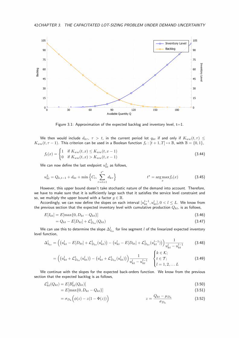
42CHAPTER 3. THE CAPACITATED LOT-SIZING PROBLEM UNDER DEMAND UNCERTAINTY
0 30 60 90 120 150 180
Available Quantity Q
0
15
30
45
60
75
90
105
Back
log
0
15
30
45
60
75
90
105In
vento
ry Le
vel
Inventory Level
Backlog
Figure 3.1: Approximation of the expected backlog and inventory level, t=1.
We then would include dkτ , τ > t, in the current period lot qkt if and only if Kww(t, τ) ≤Kww(t, τ − 1). This criterion can be used in a Boolean function ft : [t+ 1, T ] 7→ B, with B = {0, 1},
ft(x) =
{1 if Kww(t, x) ≤ Kww(t, x− 1)
0 if Kww(t, x) > Kww(t, x− 1)(3.44)
We can now define the last endpoint uLkt as follows,
uLkt = Qk,t−1 + dkt + min{Ct,
t?∑τ=t+1
dkτ
}t? = arg max
xft(x) (3.45)
However, this upper bound doesn’t take stochastic nature of the demand into account. Therefore,we have to make sure that it is sufficiently large such that it satisfies the service level constraint andso, we multiply the upper bound with a factor g ∈ R.
Accordingly, we can now define the slopes on each interval [ul−1kt , ulkt], 0 < l ≤ L. We know from
the previous section that the expected inventory level with cumulative production Qkt, is as follows,
E[Ikt] = E[max{0, Dkt −Qkt}] (3.46)
= Qkt − E[Dkt] + L1Dkt
(Qkt) (3.47)
We can use this to determine the slope ∆lIkt
for line segment l of the linearized expected inventorylevel function,
∆lIkt
=((ulkt − E[Dkt] + L1
Dkt(ulkt)
)−(ulkt − E[Dkt] + L1
Dkt(ul−1kt )
)) 1
ulkt − ul−1kt
(3.48)
=((ulkt + L1
Dkt(ulkt)
)−(ulkt + L1
Dkt(ulkt)
)) 1
ulkt − ul−1kt
k ∈ K;
t ∈ T ;
l = 1, 2, . . . L
(3.49)
We continue with the slopes for the expected back-orders function. We know from the previoussection that the expected backlog is as follows,
L1kt(Qkt) = E[Blkt(Qkt)] (3.50)
= E[max{0, Dkt −Qkt}] (3.51)
= σDk
(φ(z)− z(1− Φ(z))
)z =
Qkt − µDk
σDk
(3.52)
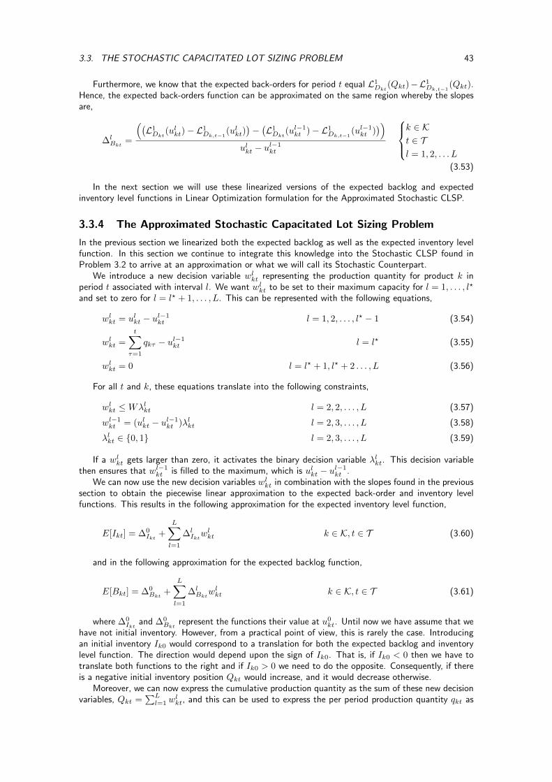
3.3. THE STOCHASTIC CAPACITATED LOT SIZING PROBLEM 43
Furthermore, we know that the expected back-orders for period t equal L1Dkt
(Qkt)−L1Dk,t−1
(Qkt).Hence, the expected back-orders function can be approximated on the same region whereby the slopesare,
∆lBkt
=
((L1Dkt
(ulkt)− L1Dk,t−1
(ulkt))−(L1Dkt
(ul−1kt )− L1Dk,t−1
(ul−1kt )))
ulkt − ul−1kt
k ∈ Kt ∈ Tl = 1, 2, . . . L
(3.53)
In the next section we will use these linearized versions of the expected backlog and expectedinventory level functions in Linear Optimization formulation for the Approximated Stochastic CLSP.
3.3.4 The Approximated Stochastic Capacitated Lot Sizing Problem
In the previous section we linearized both the expected backlog as well as the expected inventory levelfunction. In this section we continue to integrate this knowledge into the Stochastic CLSP found inProblem 3.2 to arrive at an approximation or what we will call its Stochastic Counterpart.
We introduce a new decision variable wlkt representing the production quantity for product k inperiod t associated with interval l. We want wlkt to be set to their maximum capacity for l = 1, . . . , l?
and set to zero for l = l? + 1, . . . , L. This can be represented with the following equations,
wlkt = ulkt − ul−1kt l = 1, 2, . . . , l? − 1 (3.54)
wlkt =
t∑τ=1
qkτ − ul−1kt l = l? (3.55)
wlkt = 0 l = l? + 1, l? + 2 . . . , L (3.56)
For all t and k, these equations translate into the following constraints,
wlkt ≤Wλlkt l = 2, 2, . . . , L (3.57)
wl−1kt = (ulkt − ul−1kt )λlkt l = 2, 3, . . . , L (3.58)
λlkt ∈ {0, 1} l = 2, 3, . . . , L (3.59)
If a wlkt gets larger than zero, it activates the binary decision variable λlkt. This decision variablethen ensures that wl−1kt is filled to the maximum, which is ulkt − u
l−1kt .
We can now use the new decision variables wlkt in combination with the slopes found in the previoussection to obtain the piecewise linear approximation to the expected back-order and inventory levelfunctions. This results in the following approximation for the expected inventory level function,
E[Ikt] = ∆0Ikt
+
L∑l=1
∆lIktwlkt k ∈ K, t ∈ T (3.60)
and in the following approximation for the expected backlog function,
E[Bkt] = ∆0Bkt
+
L∑l=1
∆lBkt
wlkt k ∈ K, t ∈ T (3.61)
where ∆0Ikt
and ∆0Bkt
represent the functions their value at u0kt. Until now we have assume that wehave not initial inventory. However, from a practical point of view, this is rarely the case. Introducingan initial inventory Ik0 would correspond to a translation for both the expected backlog and inventorylevel function. The direction would depend upon the sign of Ik0. That is, if Ik0 < 0 then we have totranslate both functions to the right and if Ik0 > 0 we need to do the opposite. Consequently, if thereis a negative initial inventory position Qkt would increase, and it would decrease otherwise.
Moreover, we can now express the cumulative production quantity as the sum of these new decisionvariables, Qkt =
∑Ll=1 w
lkt, and this can be used to express the per period production quantity qkt as
44CHAPTER 3. THE CAPACITATED LOT-SIZING PROBLEM UNDER DEMAND UNCERTAINTY
follows,
L∑l=1
wlkt −L∑l=1
wlk,t−1 = qkt (3.62)
Besides that, we can use the summation to introduce the inequality stating that the cumulativeproduction quantity of the previous period cannot exceed that of the current one,
L∑l=1
wlk,t−1 ≤L∑l=1
wlkt (3.63)
We can combine all of these equations, inequalities and approximations and substitute them intothe Stochastic CLSP found in Problem 3.2 to arrive at the approximated version that can be foundbelow.
Problem 3.3 (Approximated Stochastic Capacitated Lot Sizing Problem).
minT∑t=1
∑k∈K
(sckγkt + hck[∆0Ikt
+
L∑l=1
∆lIktwlkt]) +
T∑t=1
ocot (3.64)
s.t. wlkt ≤Wλlkt
k ∈ Kt ∈ Tl = 1, 2, . . . , L
(3.65)
wl−1kt = (ulkt − ul−1kt )λlkt
k ∈ Kt ∈ Tl = 2, 3, . . . , L
(3.66)
L∑l=1
wlk,t−1 ≤L∑l=1
wlkt k ∈ K, t ∈ T (3.67)
L∑l=1
wlk,t −L∑l=1
wlk,t−1 = qkt k ∈ K, t ∈ T (3.68)
qkt ≤Mγkt k ∈ K, t ∈ T (3.69)∑k∈K
tpkqkt + tskγkt ≤ Ct + ot t ∈ T (3.70)
∑ti=1E[Bki]∑ti=1E[dki]
≥ 1− βc − (1− γk,t+1) k ∈ K, t ∈ T (3.71)∑ti=1E[Bki]∑ti=1E[dki]
≤ 1− βc + (1− γk,t+1) k ∈ K, t ∈ T (3.72)
γk,T+1 = 1 k ∈ K (3.73)
γkt, λkt ∈ {0, 1}
k ∈ Kt ∈ Tl = 1, 2, . . . , L
(3.74)
λkt ∈ {0, 1}
k ∈ Kt ∈ Tl = 2, 3, . . . , L
(3.75)
wkt ≥ 0
k ∈ Kt ∈ Tl = 1, 2, . . . , L
(3.76)
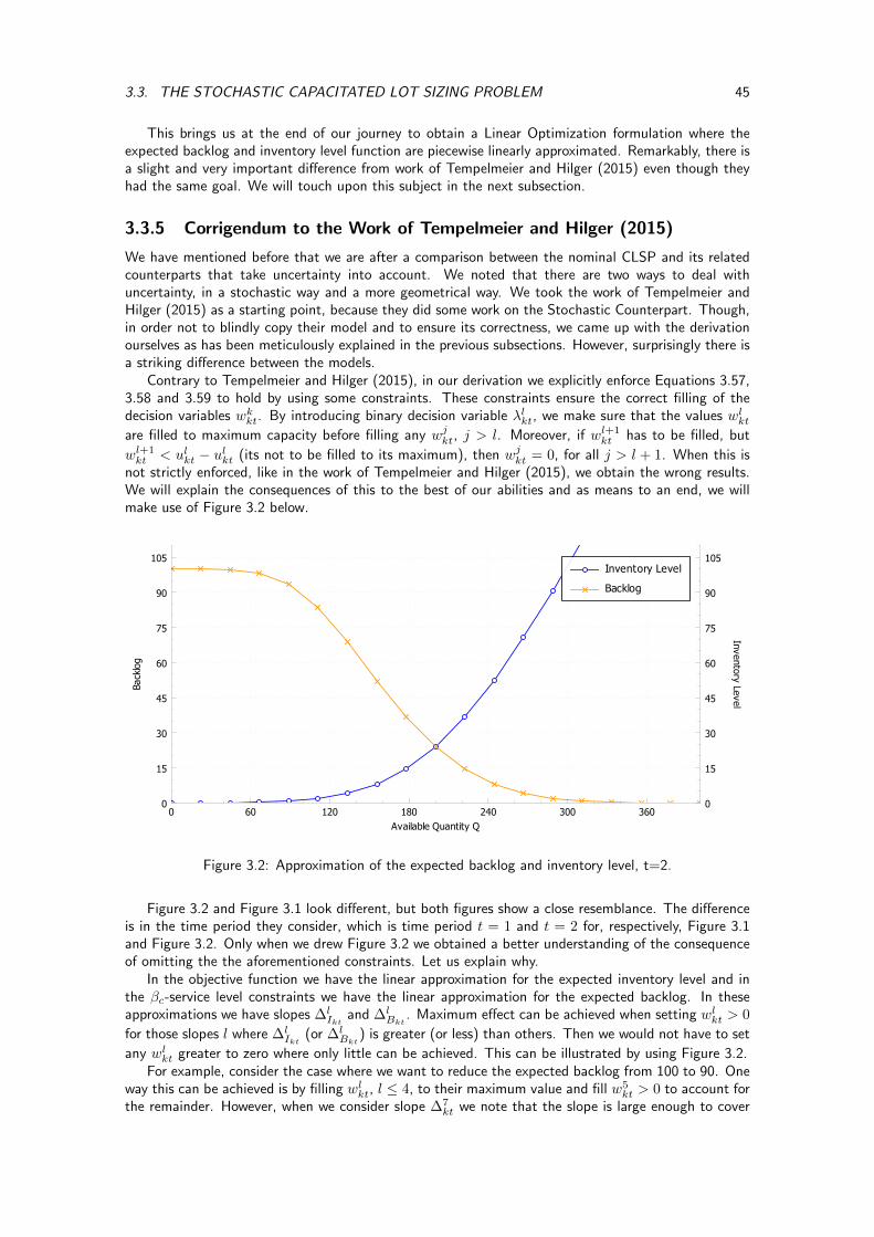
3.3. THE STOCHASTIC CAPACITATED LOT SIZING PROBLEM 45
This brings us at the end of our journey to obtain a Linear Optimization formulation where theexpected backlog and inventory level function are piecewise linearly approximated. Remarkably, there isa slight and very important difference from work of Tempelmeier and Hilger (2015) even though theyhad the same goal. We will touch upon this subject in the next subsection.
3.3.5 Corrigendum to the Work of Tempelmeier and Hilger (2015)
We have mentioned before that we are after a comparison between the nominal CLSP and its relatedcounterparts that take uncertainty into account. We noted that there are two ways to deal withuncertainty, in a stochastic way and a more geometrical way. We took the work of Tempelmeier andHilger (2015) as a starting point, because they did some work on the Stochastic Counterpart. Though,in order not to blindly copy their model and to ensure its correctness, we came up with the derivationourselves as has been meticulously explained in the previous subsections. However, surprisingly there isa striking difference between the models.
Contrary to Tempelmeier and Hilger (2015), in our derivation we explicitly enforce Equations 3.57,3.58 and 3.59 to hold by using some constraints. These constraints ensure the correct filling of thedecision variables wkkt. By introducing binary decision variable λlkt, we make sure that the values wlktare filled to maximum capacity before filling any wjkt, j > l. Moreover, if wl+1
kt has to be filled, but
wl+1kt < ulkt − ulkt (its not to be filled to its maximum), then wjkt = 0, for all j > l + 1. When this is
not strictly enforced, like in the work of Tempelmeier and Hilger (2015), we obtain the wrong results.We will explain the consequences of this to the best of our abilities and as means to an end, we willmake use of Figure 3.2 below.
0 60 120 180 240 300 360
Available Quantity Q
0
15
30
45
60
75
90
105
Back
log
0
15
30
45
60
75
90
105
Invento
ry Le
vel
Inventory Level
Backlog
Figure 3.2: Approximation of the expected backlog and inventory level, t=2.
Figure 3.2 and Figure 3.1 look different, but both figures show a close resemblance. The differenceis in the time period they consider, which is time period t = 1 and t = 2 for, respectively, Figure 3.1and Figure 3.2. Only when we drew Figure 3.2 we obtained a better understanding of the consequenceof omitting the the aforementioned constraints. Let us explain why.
In the objective function we have the linear approximation for the expected inventory level and inthe βc-service level constraints we have the linear approximation for the expected backlog. In theseapproximations we have slopes ∆l
Iktand ∆l
Bkt. Maximum effect can be achieved when setting wlkt > 0
for those slopes l where ∆lIkt
(or ∆lBkt
) is greater (or less) than others. Then we would not have to set
any wlkt greater to zero where only little can be achieved. This can be illustrated by using Figure 3.2.For example, consider the case where we want to reduce the expected backlog from 100 to 90. One
way this can be achieved is by filling wlkt, l ≤ 4, to their maximum value and fill w5kt > 0 to account for
the remainder. However, when we consider slope ∆7kt we note that the slope is large enough to cover
46CHAPTER 3. THE CAPACITATED LOT-SIZING PROBLEM UNDER DEMAND UNCERTAINTY
the desired 10 units decrease in the expected backlog right away. Hence, if we only fill w7kt we would
still achieve the 10 units decrease, but produce significantly less. This is an interesting insight, becauseapparently we can reduce the expected backlog by “producing” less and this is of interest, because weincur setup costs if we want to produce and inventory holding costs for excessive amounts of productsproduced. Please, note that this way of hacking the model does not violate any of the constraints.
Now we know that we do not necessarily have to “produce” a lot to significantly reduce the expectedbacklog function, we just have to choose the intervals that correspond to steep slopes. From thedefinition of the βc-service level constraint we know that a reduction in the expected backlog functioncorresponds to a better service level. This is a desirable effect and the insight obtained above wouldimply that we can do so by producing less. Of course, is should be duly noted that this is abuse ofterms in some sense, because setting wlkt larger than zero does not necessarily corresponds to producingproducts. The result is interesting, to say the least, but its consequence became fully clear during anextensive investigation of this problem by means of a simulation study.
The simulation study confirmed the idea that the Tempelmeier and Hilger (2015) selectively fills wlkt,i.e. they are not filled to their maximum for increasing numbers in l. Moreover, it does so while satisfyingeach of the constraints, also the service level constraint. First of all, it fills those wlkt that reduces the
expected backlog the most, but second it manages to let the constraint∑Ll=1 w
lk,t−
∑Ll=1 w
lk,t−1 = qkt,
result in zero production for 2 ≤ t. This is because for t = 1 the constraint would read∑Ll=1 w
lk,t = qkt
and we have some products k produced. However, since we are able to freely chose wlkt, it is possible
to let∑Ll=1 w
lk,t −
∑Ll=1 w
lk,t−1 = qkt = 0. Consequently, we do not have any setup costs in periods
2 ≤ t, because qkt = 0 in those periods. We can conclude that the model of Tempelmeier and Hilger(2015) has its flaws, because it does not strictly enforce the wlkt to be filled in the correct way. Clearly,the constraints mentioned above are of utmost importance and should be incorporated in a stochasticapproximation to the CLSP for things to work out correctly.
3.4 A Robust Counterpart of the Capacitated Lot Sizing Prob-lem under Interval Uncertainty
Deriving the robust counterpart of the nominal CLSP introduced in Problem 3.1 is rather straightforward based on the knowledge we obtained in the previous chapter. In a similar fashion as has beendone in case of the single item production planning problem, can derive the Robust Counterpart.
We start from the nominal CLSP found in Problem 3.1. In typical formulations of the CLSP theincentive to produce comes from the fact that negative inventory is not allowed. However, as we haveexplained before, negative inventory, or back-orders, are unavoidable in the case of demand uncertainty.If demand for each product is identically and independently normally distributed and we want to havezero expected back-orders each period, then we should have an infinite amount of inventory. In case ofstochastic uncertainty we have introduced the βc-service level as an incentive to produce. In case ofthe robust approach we will rely on the back-order cost parameter.
In the nominal CLSP problem we can introduce uncertainty by means of uncertainty sets. In our casewe will only restrict ourselves to the most conservative Robust Counterpart, i.e. taking the l∞-norm onthe demand which is otherwise known as interval uncertainty. This means that the per period demandranges with a certain interval, dt ∈ [dt − dt, dt − dt]. More formally, like before, the demand vector isparameterized in an affine fashion by the perturbation vectors,
d(ζ) = d0 +
T∑t=1
dtζt ‖ζ‖∞ ≤ 1 (3.77)
In a similar way as before, we have the following uncertainty set U∞,
U∞ =
{d = d0 +
T∑t=1
ζtdt : ζ ∈ Z = {ζ ∈ RT : ‖ζ‖∞ ≤ 1} ⊂ RT
}(3.78)
We can substitute this uncertainty set in Problem 3.1 to arrive at,
3.5. CONCLUSION 47
Problem 3.4 (Uncertain Capacitated Lot Sizing Problem).
minT∑t=1
∑k∈K
(sckγkt + ykt) +
T∑t=1
ocot (3.79)
s.t. hck
(Ik0 +
t∑s=1
qks −t∑
s=1
dks
)≤ ykt ∀d ∈ U∞, k ∈ K, t ∈ T (3.80)
− bck(Ik0 +
t∑s=1
qks −t∑
s=1
dks
)≤ ykt ∀d ∈ U∞, k ∈ K, t ∈ T (3.81)
qkt ≤Mγkt k ∈ K, t ∈ T (3.82)∑k∈K
(tpkqkt + tskγkt) ≤ Ct + ot t ∈ T (3.83)
γkt ∈ {0, 1} k ∈ K, t ∈ T (3.84)
qkt, ot ≥ 0 k ∈ K, t ∈ T (3.85)
We have uncertainty in exactly the same constraints as we had in the previous chapter. The onlydifference is that we have k of such constraints, for each product one. Since the other constraints arenot affected by the uncertainty, we can leave them out of consideration with regards to determining theRobust Counterpart of the problem above. This means that we can borrow heavily from the derivationin the previous chapter to come up with the Robust Counterpart found in Problem 3.5 below,
Problem 3.5 (Robust Counterpart Capacitated Lot Sizing Problem with an l∞-norm).
minT∑t=1
∑k∈K
(sckγkt + ykt) +
T∑t=1
ocot (3.86)
s.t. hck
(Ik0 +
t∑s=1
qks −t∑
s=1
dkszks +
t∑s=1
ωks
)≤ ykt k ∈ K, t ∈ T (3.87)
− bck(Ik0 +
t∑s=1
qks −t∑
s=1
dkszks −t∑
s=1
ωks
)≤ ykt k ∈ K, t ∈ T (3.88)
− ωkt ≤ dktzkt ≤ ωkt k ∈ K, t ∈ T (3.89)
qkt ≤Mγkt k ∈ K, t ∈ T (3.90)∑k∈K
(tpkqkt + tskγkt) ≤ Ct + ot t ∈ T (3.91)
γkt ∈ {0, 1} k ∈ K, t ∈ T (3.92)
zt = 1 k ∈ K, t ∈ T (3.93)
qkt, ot ≥ 0 k ∈ K, t ∈ T (3.94)
3.5 Conclusion
In this chapter we discussed models for the CLSP in case of deterministic demand and uncertaindemand. We started by discussing the case where demand is known in advance and this has led to thenominal problem. We have seen that for computational reasons various heuristics have been developed.Nevertheless, we stayed with mathematical programming formulations and basically, we extended theproduction planning problem of the pervious chapter by considering multiple items, setup costs andpossibly, setup times.
We introduced demand uncertainty in the nominal problem in two ways. First, we took a stochasticapproach and second, we took a Robust Optimization approach. The introduction of demand uncer-tainty gave rise to a challenge, because if demand would realize in such a way that we can’t satisfy it,we would end up in having back-orders. However, only a certain amount of back-orders is allowed andthis may mean that the βc-service level could be violated if there is not enough capacity. Therefore, we
48CHAPTER 3. THE CAPACITATED LOT-SIZING PROBLEM UNDER DEMAND UNCERTAINTY
relaxed the problem by introducing overtime. We meticulously described the derivation of the stochasticcounterpart as well as flaws that were discovered in existing approaches.
At last, we took a Robust Optimization approach to the problem and introduced interval demanduncertainty. The derivation of the robust Counterpart was merely a straight forward execution of thesame steps taken in the previous chapter, because most of the complexities were already discussed thatchapter.
So, we have been able to formulate the a Stochastic and Robust Counterpart of the nominal CLSP.This means that we can confirm two more of our research questions. In the next chapter we will comparethe models introduced in this chapter to assess their performance in case of demand uncertainty duringa simulation study in a rolling horizon setting.
Chapter 4
Simulation Study
4.1 Introduction
This chapter deals with a comparison between the models that we have introduced in the previouschapter for solving the Capacitated Lot Sizing Problem. Our primary goal is to achieve a certain β-service level for a product when demand is uncertain and secondary to that we will try to minimizethe costs involved. Hence, we are interested in the model that achieves the required service level atminimum cost. Since we investigate how these models perform under demand uncertainty, we expect theStochastic and Robust Counterpart of the nominal problem to perform better under demand uncertaintythan the nominal problem, because both have mechanisms to deal with uncertainty.
In order to establish statistically significant results, we conducted a simulation study. In this studywe run the various production planning models in a rolling horizon setting. We start this chapter withdiscussing the methodology behind this simulation study. We will explain the type of simulation studyconducted, convince you as reader about the validity of the implementation of the models, explain thesimulation framework we have build and the statistics we will measure. Thereafter, we continue withexperimental design and the results we have obtained.
4.2 Methodology
4.2.1 A Discrete-Event Simulation in a Rolling Horizon Setting
By definition of Law (2015, pp. 5-6), we conduct a dynamic, stochastic, discrete-event simulation whichin our case concerns the modeling of a production system as it evolves over time. State variables suchas the inventory level change instantaneously and at only a countable number of points in time, i.e. ourreview period. The stochastic component stems from the fact that demand is uncertain and randomlydistributed. We will assume demand to be identically and independently normally distributed. However,the distribution is truncated such that no demand will be realized lower than zero, i.e. negative demandis not allowed.
We will employ our lot sizing models in a rolling horizon setting. The reason for this is becuaseprevious research by Drexl and Kimms (1997) and Helber et al. (2013) suggest that research should bedone on how lot sizing models perform in a rolling horizon setting. Furthermore, lot sizing models areinherently employed in practice in a rolling horizon setting. Therefore, in order to asses the whether ornot our models are suitable for practice we have to simulate them in a rolling horizon setting.
In essence, a rolling horizon settings means the following. At t = 1, we have a finite planninghorizon [t, t+T −1] for which we want to determine the lot sizes. We employ our models and receive aproduction plan. Of the resulting production plan we have to commit the first Tc periods. With commitwe mean that we have to implement production for these periods and even as time increases and newinformation comes available, we are not allowed to alter the production quantities set for those specificperiods. Hence, after we have planned production, we observe the next Tc periods before planningproduction again. This means that we have rolled Tc periods forward. We continue to roll forward aslong as t+T ≤ H. Note, it goes without saying that all models will be subject to the same realizations
49
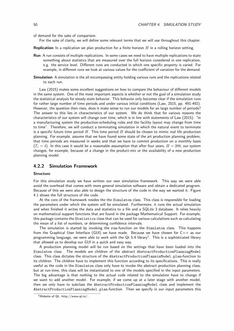
50 CHAPTER 4. SIMULATION STUDY
of demand for the sake of comparison.For the sake of clarity, we will define some relevant terms that we will use throughout this chapter.
Replication In a replication we plan production for a finite horizon H in a rolling horizon setting.
Run A run consists of multiple replications. In some cases we need to have multiple replications to statesomething about statistics that are measured over the full horizon considered in one replication,e.g. the service level. Different runs are conducted in which one specific property is varied. Forexample, in different runs we look at various values for the coefficient of variation for the demand.
Simulation A simulation is the all encompassing entity holding various runs and the replications relatedto each run.
Law (2015) makes some excellent suggestions on how to compare the behaviour of different modelsin the same system. One of the most important aspects is whether or not the goal of a simulation studythe statistical analysis for steady state behavior. This behavior only becomes clear if the simulation runsfor rather large number of time periods and under various initial conditions (Law, 2015, pp. 491-492).However, the question then rises, does it make sense to run our models for an large number of periods?The answer to this lies in characteristics of our system. We do think that for various reasons thecharacteristics of our system will change over time, which is in line with statements of Law (2015): “ina manufacturing system the production-scheduling rules and the facility layout may change from timeto time”. Therefore, we will conduct a terminating simulation in which the natural event to terminateis a specific future time period H. This time period H should be chosen to mimic real life productionplanning. For example, assume that we have found some state of the art production planning problem,that time periods are measured in weeks and that we have to commit production on a monthly basis(Tc = 4). In this case it would be a reasonable assumption that after four years, H = 208, our systemchanges, for example, because of a change in the product-mix or the availability of a new productionplanning model.
4.2.2 Simulation Framework
Structure
For this simulation study we have written our own simulation framework. This way we were ableavoid the overhead that comes with more general simulation software and obtain a dedicated program.Because of this we were also able to design the structure of the code in the way we wanted it. Figure4.1 shows the full structure of the code.
At the core of the framework resides the the Simulaton class. This class is responsible for loadingthe parameters under which the system will be simulated. Furthermore, it runs the actual simulationand when finished it writes the data and statistics to a file and a SQLite 3 database. It relies heavilyon mathematical support functions that are found in the package Mathematical Support. For example,this package contains the Statistics class that can be used for various calculations such as calculatingthe mean of a list of numbers, or determining confidence intervals.
The simulation is started by invoking the run-function on the Simulaton class. This happensfrom the Graphical User Interface (GUI) we have made. Because we have chosen for C++ as ourprogramming language, we were able to work with the Qt 5.4 library1. This is a sophisticated librarythat allowed us to develop our GUI in a quick and easy way.
A production planning model will be run based on the settings that have been loaded into theSimulaton class. The models are children of the abstract AbstractProductionPlanningModel
class. This class dictates the structure of the AbstractProductionPlanninModel.plan-function toits children. The children have to implement this function according to its specifications. This is reallyuseful as the code in the Simulaton class only have to invoke the abstract production planning class,but at run-time, this class will be instantiated to one of the models specified in the input parameters.The big advantage is that nothing to the actual code related to the simulation have to change ifwe want to add another model. For example, if we come up at a later stage with another model,then we only have to subclass the AbstractProductionPlanningModel class and implement theAbstractProductionPlanningModel.plan-function. Then we specify in our input parameters this
1Website of Qt: http://www.qt.io/.
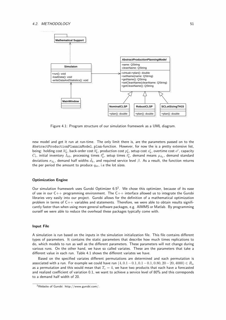
4.2. METHODOLOGY 51
AbstractProductionPlanningModel
-name: QString-cleanName: QString
«virtual»+plan(): double+setName(name: QString)+getName(): QString+setCleanName(cleanName: QString)+getCleanName(): QString
NominalCLSP
+plan(): double
RobustCLSP
+plan(): double
SCLotSizingTH15
+plan(): double
Simulaton
+run(): void-loadData(): void-writeDataAndStatistics(): void
MainWindow
Mathematical Support
Model::Main
Figure 4.1: Program structure of our simulation framework as a UML diagram.
new model and get it run at run-time. The only limit there is, are the parameters passed on to theAbstractProductionPlanninModel.plan-function. However, for now the is a pretty extensive list,being: holding cost hck, back-order cost bck, production cost pck, setup cost sck, overtime cost oc, capacityCt, initial inventory Ik0, processing times tpk, setup times tsk, demand means µdk , demand standard
deviations σdk , demand half widths dk, and required service level β. As a result, the function returnsthe per period the amount to produce qkt, i.e the lot sizes.
Optimization Engine
Our simulation framework uses Gurobi Optimizer 6.52. We chose this optimizer, because of its easeof use in our C++ programming environment. The C++ interface allowed us to integrate the Gurobilibraries very easily into our project. Gurobi allows for the definition of a mathematical optimizationproblem in terms of C++ variables and statements. Therefore, we were able to obtain results signifi-cantly faster than when using more general software packages, e.g. AIMMS or Matlab. By programmingourself we were able to reduce the overhead these packages typically come with.
Input File
A simulation is run based on the inputs in the simulation initialization file. This file contains differenttypes of parameters. It contains the static parameters that describe how much times replications todo, which models to run as well as the different parameters. These parameters will not change duringvarious runs. On the other hand, we have so called variates. These are the parameters that take adifferent value in each run. Table 4.1 shows the different variates we have.
Based on the specified variates different permutations are determined and each permutation isassociated with a run. For example we could have run (4, 0.1−0.1, 0.1−0.1, 0.80, 20−20, 4000) ∈ Rnas a permutation and this would mean that Tc = 4, we have two products that each have a forecastedand realized coefficient of variation 0.1, we want to achieve a service level of 80% and this correspondsto a demand half width of 20.
2Website of Gurobi: http://www.gurobi.com/.
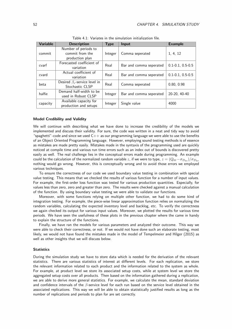
52 CHAPTER 4. SIMULATION STUDY
Table 4.1: Variates in the simulation initialization file.
Variable Description Type Input Example
commitNumber of periods to
commit from theproduction plan
Integer Comma seperated 1, 4, 12
cvarfForecasted coefficient of
variationReal Bar and comma seperated 0.1-0.1, 0.5-0.5
cvardActual coefficient of
variationReal Bar and comma seperated 0.1-0.1, 0.5-0.5
betaDesired βc-service level in
Stochastic CLSPReal Comma seperated 0.80, 0.98
halfieDemand half-width to be
used in Robust CLSPInteger Bar and comma seperated 20-20, 40-40
capacityAvailable capacity forproduction and setups
Integer Single value 4000
Model Credibility and Validity
We will continue with describing what we have done to increase the credibility of the models weimplemented and discuss their validity. For sure, the code was written in a neat and tidy way to avoid“spaghetti”-code and since we used C++ as our programming language we were able to use the benefitsof an Object Oriented Programming language. However, employing sound testing methods is of essenceas mistakes are made pretty easily. Mistakes made in the syntaxis of the programming used are quicklynoticed at compile time and various run time errors such as an index out of bounds is discovered prettyeasily as well. The real challenge lies in the conceptual errors made during programming. An examplecould be the calculation of the normalized random variable z, if we were to type, z = (Qkt−σDkt
)/σDkt
nothing would go wrong. However, this is conceptually wrong and to avoid those errors we employedvarious techniques.
To ensure the correctness of our code we used boundary value testing in combination with specialvalue testing. This means that we checked the results of various function for a number of input values.For example, the first-order loss function was tested for various production quantities. Especially, forvalues less than zero, zero and greater than zero. The results were checked against a manual calculationof the function. By using boundary value testing we were able to validate our functions.
Moreover, with some functions relying on multiple other function, we had to do some kind ofintegration testing. For example, the piece-wise linear approximation function relies on normalizing therandom variables, calculating the expected inventory level and backlog, etc. To verify the correctnesswe again checked its output for various input values. Moreover, we plotted the results for various timeperiods. We have seen the usefulness of these plots in the previous chapter where the came in handyto explain the structure of the functions.
Finally, we have ran the models for various parameters and analyzed their outcome. This way wewere able to check their correctness, or not. If we would not have done such an elaborate testing, mostlikely, we would not have found the mistakes made in the model of Tempelmeier and Hilger (2015) aswell as other insights that we will discuss below.
Statistics
During the simulation study we have to store data which is needed for the derivation of the relevantstatistics. There are various statistics of interest at different levels. For each replication, we storethe relevant information related to each product and the information related to the system as whole.For example, at product level we store its associated setup costs, while at system level we store theaggregated setup costs over all products. Then based on the information gathered during a replication,we are able to derive more general statistics. For example, we calculate the mean, standard deviationand confidence intervals of the β-service level for each run based on the service level obtained in theassociated replications. This way we will be able to obtain statistically justified results as long as thenumber of replications and periods to plan for are set correctly.
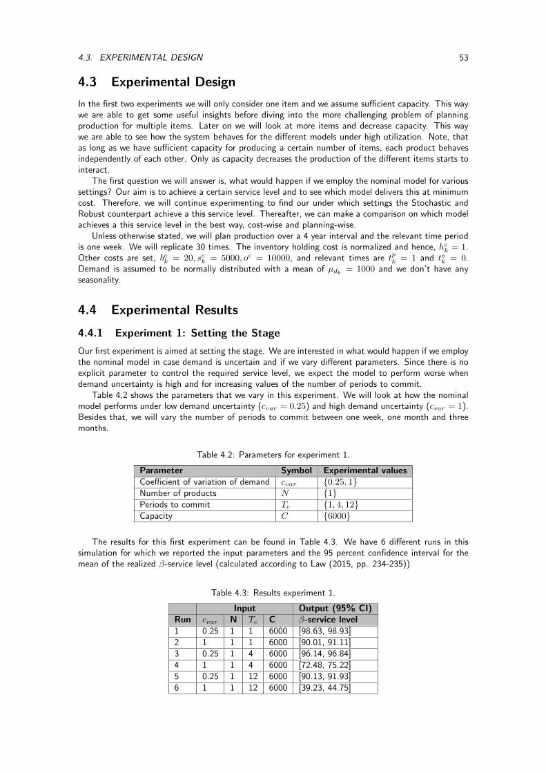
4.3. EXPERIMENTAL DESIGN 53
4.3 Experimental Design
In the first two experiments we will only consider one item and we assume sufficient capacity. This waywe are able to get some useful insights before diving into the more challenging problem of planningproduction for multiple items. Later on we will look at more items and decrease capacity. This waywe are able to see how the system behaves for the different models under high utilization. Note, thatas long as we have sufficient capacity for producing a certain number of items, each product behavesindependently of each other. Only as capacity decreases the production of the different items starts tointeract.
The first question we will answer is, what would happen if we employ the nominal model for varioussettings? Our aim is to achieve a certain service level and to see which model delivers this at minimumcost. Therefore, we will continue experimenting to find our under which settings the Stochastic andRobust counterpart achieve a this service level. Thereafter, we can make a comparison on which modelachieves a this service level in the best way, cost-wise and planning-wise.
Unless otherwise stated, we will plan production over a 4 year interval and the relevant time periodis one week. We will replicate 30 times. The inventory holding cost is normalized and hence, hck = 1.Other costs are set, bck = 20, sck = 5000, oc = 10000, and relevant times are tpk = 1 and tsk = 0.Demand is assumed to be normally distributed with a mean of µdk = 1000 and we don’t have anyseasonality.
4.4 Experimental Results
4.4.1 Experiment 1: Setting the Stage
Our first experiment is aimed at setting the stage. We are interested in what would happen if we employthe nominal model in case demand is uncertain and if we vary different parameters. Since there is noexplicit parameter to control the required service level, we expect the model to perform worse whendemand uncertainty is high and for increasing values of the number of periods to commit.
Table 4.2 shows the parameters that we vary in this experiment. We will look at how the nominalmodel performs under low demand uncertainty (cvar = 0.25) and high demand uncertainty (cvar = 1).Besides that, we will vary the number of periods to commit between one week, one month and threemonths.
Table 4.2: Parameters for experiment 1.
Parameter Symbol Experimental valuesCoefficient of variation of demand cvar {0.25, 1}Number of products N {1}Periods to commit Tc {1, 4, 12}Capacity C {6000}
The results for this first experiment can be found in Table 4.3. We have 6 different runs in thissimulation for which we reported the input parameters and the 95 percent confidence interval for themean of the realized β-service level (calculated according to Law (2015, pp. 234-235))
Table 4.3: Results experiment 1.
Input Output (95% CI)Run cvar N Tc C β-service level1 0.25 1 1 6000 [98.63, 98.93]2 1 1 1 6000 [90.01, 91.11]3 0.25 1 4 6000 [96.14, 96.84]4 1 1 4 6000 [72.48, 75.22]5 0.25 1 12 6000 [90.13, 91.93]6 1 1 12 6000 [39.23, 44.75]
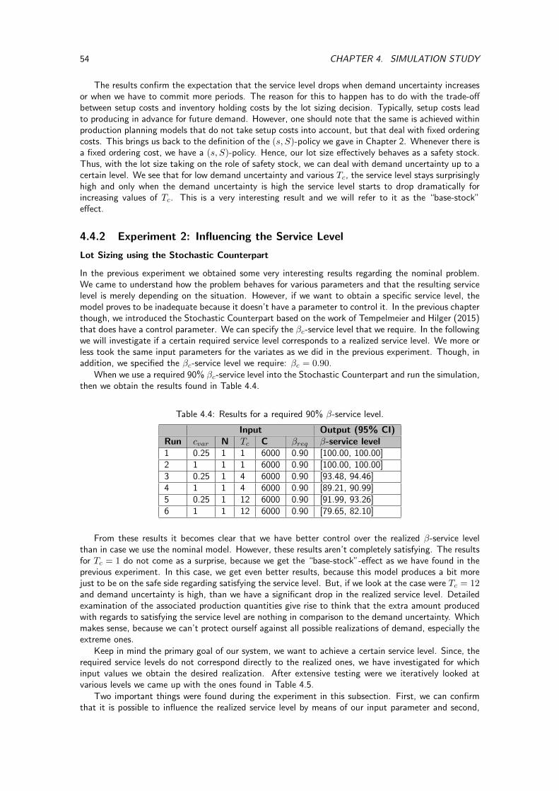
54 CHAPTER 4. SIMULATION STUDY
The results confirm the expectation that the service level drops when demand uncertainty increasesor when we have to commit more periods. The reason for this to happen has to do with the trade-offbetween setup costs and inventory holding costs by the lot sizing decision. Typically, setup costs leadto producing in advance for future demand. However, one should note that the same is achieved withinproduction planning models that do not take setup costs into account, but that deal with fixed orderingcosts. This brings us back to the definition of the (s, S)-policy we gave in Chapter 2. Whenever there isa fixed ordering cost, we have a (s, S)-policy. Hence, our lot size effectively behaves as a safety stock.Thus, with the lot size taking on the role of safety stock, we can deal with demand uncertainty up to acertain level. We see that for low demand uncertainty and various Tc, the service level stays surprisinglyhigh and only when the demand uncertainty is high the service level starts to drop dramatically forincreasing values of Tc. This is a very interesting result and we will refer to it as the “base-stock”effect.
4.4.2 Experiment 2: Influencing the Service Level
Lot Sizing using the Stochastic Counterpart
In the previous experiment we obtained some very interesting results regarding the nominal problem.We came to understand how the problem behaves for various parameters and that the resulting servicelevel is merely depending on the situation. However, if we want to obtain a specific service level, themodel proves to be inadequate because it doesn’t have a parameter to control it. In the previous chapterthough, we introduced the Stochastic Counterpart based on the work of Tempelmeier and Hilger (2015)that does have a control parameter. We can specify the βc-service level that we require. In the followingwe will investigate if a certain required service level corresponds to a realized service level. We more orless took the same input parameters for the variates as we did in the previous experiment. Though, inaddition, we specified the βc-service level we require: βc = 0.90.
When we use a required 90% βc-service level into the Stochastic Counterpart and run the simulation,then we obtain the results found in Table 4.4.
Table 4.4: Results for a required 90% β-service level.
Input Output (95% CI)Run cvar N Tc C βreq β-service level1 0.25 1 1 6000 0.90 [100.00, 100.00]2 1 1 1 6000 0.90 [100.00, 100.00]3 0.25 1 4 6000 0.90 [93.48, 94.46]4 1 1 4 6000 0.90 [89.21, 90.99]5 0.25 1 12 6000 0.90 [91.99, 93.26]6 1 1 12 6000 0.90 [79.65, 82.10]
From these results it becomes clear that we have better control over the realized β-service levelthan in case we use the nominal model. However, these results aren’t completely satisfying. The resultsfor Tc = 1 do not come as a surprise, because we get the “base-stock”-effect as we have found in theprevious experiment. In this case, we get even better results, because this model produces a bit morejust to be on the safe side regarding satisfying the service level. But, if we look at the case were Tc = 12and demand uncertainty is high, than we have a significant drop in the realized service level. Detailedexamination of the associated production quantities give rise to think that the extra amount producedwith regards to satisfying the service level are nothing in comparison to the demand uncertainty. Whichmakes sense, because we can’t protect ourself against all possible realizations of demand, especially theextreme ones.
Keep in mind the primary goal of our system, we want to achieve a certain service level. Since, therequired service levels do not correspond directly to the realized ones, we have investigated for whichinput values we obtain the desired realization. After extensive testing were we iteratively looked atvarious levels we came up with the ones found in Table 4.5.
Two important things were found during the experiment in this subsection. First, we can confirmthat it is possible to influence the realized service level by means of our input parameter and second,
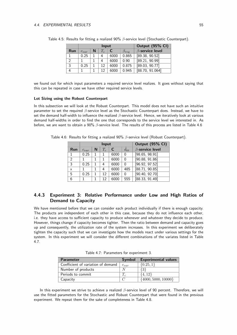
4.4. EXPERIMENTAL RESULTS 55
Table 4.5: Results for fitting a realized 90% β-service level (Stochastic Counterpart).
Input Output (95% CI)Run cvar N Tc C βreq β-service level1 0.25 1 4 6000 0.865 [89.38, 90.52]2 1 1 4 6000 0.90 [89.21, 90.99]3 0.25 1 12 6000 0.875 [89.03, 90.77]4 1 1 12 6000 0.945 [88.70, 91.064]
we found out for which input parameters a required service level realizes. It goes without saying thatthis can be repeated in case we have other required service levels.
Lot Sizing using the Robust Counterpart
In this subsection we will look at the Robust Counterpart. This model does not have such an intuitiveparameter to set the required β-service level as the Stochastic Counterpart does. Instead, we have toset the demand half-width to influence the realized β-service level. Hence, we iteratively look at variousdemand half-widths in order to find the one that corresponds to the service level we interested in. Asbefore, we are want to obtain a 90% β-service level. The results of this process are listed in Table 4.6
Table 4.6: Results for fitting a realized 90% β-service level (Robust Counterpart).
Input Output (95% CI)
Run cvar N Tc C dkt β-service level1 0.25 1 1 6000 0 [98.65, 98.91]2 1 1 1 6000 0 [90.88, 91.86]3 0.25 1 4 6000 0 [96.92, 97.52]x 1 1 4 6000 485 [88.71, 90.85]5 0.25 1 12 6000 0 [90.40, 92.70]6 1 1 12 6000 555 [88.33, 91.49]
4.4.3 Experiment 3: Relative Performance under Low and High Ratios ofDemand to Capacity
We have mentioned before that we can consider each product individually if there is enough capacity.The products are independent of each other in this case, because they do not influence each other,i.e. they have access to sufficient capacity to produce whenever and whatever they decide to produce.However, things change if capacity becomes tighter. Then the ratio between demand and capacity goesup and consequently, the utilization rate of the system increases. In this experiment we deliberatelytighten the capacity such that we can investigate how the models react under various settings for thesystem. In this experiment we will consider the different combinations of the variates listed in Table4.7.
Table 4.7: Parameters for experiment 3.
Parameter Symbol Experimental valuesCoefficient of variation of demand cvar {0.25, 1}Number of products N {3}Periods to commit Tc {4, 12}Capacity C {4000, 5000, 10000}
In this experiment we strive to achieve a realized β-service level of 90 percent. Therefore, we willuse the fitted parameters for the Stochastic and Robust Counterpart that were found in the previousexperiment. We repeat them for the sake of completeness in Table 4.8.
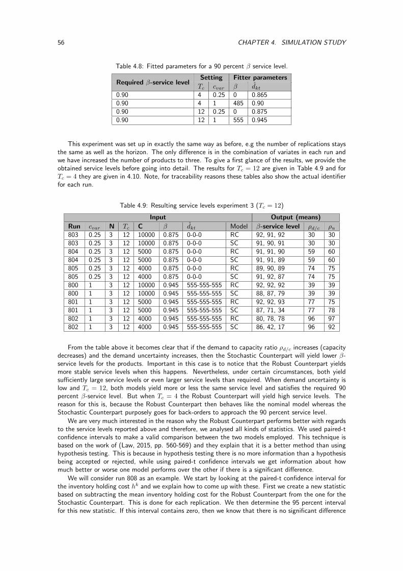
56 CHAPTER 4. SIMULATION STUDY
Table 4.8: Fitted parameters for a 90 percent β service level.
Setting Fitter parametersRequired β-service level
Tc cvar β dkt0.90 4 0.25 0 0.8650.90 4 1 485 0.900.90 12 0.25 0 0.8750.90 12 1 555 0.945
This experiment was set up in exactly the same way as before, e.g the number of replications staysthe same as well as the horizon. The only difference is in the combination of variates in each run andwe have increased the number of products to three. To give a first glance of the results, we provide theobtained service levels before going into detail. The results for Tc = 12 are given in Table 4.9 and forTc = 4 they are given in 4.10. Note, for traceability reasons these tables also show the actual identifierfor each run.
Table 4.9: Resulting service levels experiment 3 (Tc = 12)
Input Output (means)
Run cvar N Tc C β dkt Model β-service level ρd/c ρu803 0.25 3 12 10000 0.875 0-0-0 RC 92, 91, 92 30 30803 0.25 3 12 10000 0.875 0-0-0 SC 91, 90, 91 30 30804 0.25 3 12 5000 0.875 0-0-0 RC 91, 91, 90 59 60804 0.25 3 12 5000 0.875 0-0-0 SC 91, 91, 89 59 60805 0.25 3 12 4000 0.875 0-0-0 RC 89, 90, 89 74 75805 0.25 3 12 4000 0.875 0-0-0 SC 91, 92, 87 74 75800 1 3 12 10000 0.945 555-555-555 RC 92, 92, 92 39 39800 1 3 12 10000 0.945 555-555-555 SC 88, 87, 79 39 39801 1 3 12 5000 0.945 555-555-555 RC 92, 92, 93 77 75801 1 3 12 5000 0.945 555-555-555 SC 87, 71, 34 77 78802 1 3 12 4000 0.945 555-555-555 RC 80, 78, 78 96 97802 1 3 12 4000 0.945 555-555-555 SC 86, 42, 17 96 92
From the table above it becomes clear that if the demand to capacity ratio ρd/c increases (capacitydecreases) and the demand uncertainty increases, then the Stochastic Counterpart will yield lower β-service levels for the products. Important in this case is to notice that the Robust Counterpart yieldsmore stable service levels when this happens. Nevertheless, under certain circumstances, both yieldsufficiently large service levels or even larger service levels than required. When demand uncertainty islow and Tc = 12, both models yield more or less the same service level and satisfies the required 90percent β-service level. But when Tc = 4 the Robust Counterpart will yield high service levels. Thereason for this is, because the Robust Counterpart then behaves like the nominal model whereas theStochastic Counterpart purposely goes for back-orders to approach the 90 percent service level.
We are very much interested in the reason why the Robust Counterpart performs better with regardsto the service levels reported above and therefore, we analysed all kinds of statistics. We used paired-tconfidence intervals to make a valid comparison between the two models employed. This technique isbased on the work of (Law, 2015, pp. 560-569) and they explain that it is a better method than usinghypothesis testing. This is because in hypothesis testing there is no more information than a hypothesisbeing accepted or rejected, while using paired-t confidence intervals we get information about howmuch better or worse one model performs over the other if there is a significant difference.
We will consider run 808 as an example. We start by looking at the paired-t confidence interval forthe inventory holding cost hk and we explain how to come up with these. First we create a new statisticbased on subtracting the mean inventory holding cost for the Robust Counterpart from the one for theStochastic Counterpart. This is done for each replication. We then determine the 95 percent intervalfor this new statistic. If this interval contains zero, then we know that there is no significant difference
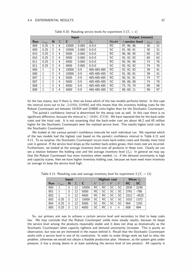
4.4. EXPERIMENTAL RESULTS 57
Table 4.10: Resulting service levels for experiment 3 (Tc = 4)
Input Output (means)
Run cvar N Tc C β dkt Model β-service level ρd/c ρu809 0.25 3 4 10000 0.865 0-0-0 RC 97, 96, 96 30 31809 0.25 3 4 10000 0.865 0-0-0 SC 91, 90, 91 30 31810 0.25 3 4 5000 0.865 0-0-0 RC 96, 96, 95 60 62810 0.25 3 4 5000 0.865 0-0-0 SC 92, 92, 92 60 62811 0.25 3 4 4000 0.865 0-0-0 RC 95, 95, 96 74 76811 0.25 3 4 4000 0.865 0-0-0 SC 92, 92, 92 74 76806 1 3 4 10000 0.9 485-485-485 RC 92, 92, 92 39 41806 1 3 4 10000 0.9 485-485-485 SC 91, 90, 91 39 41807 1 3 4 5000 0.9 485-485-485 RC 90, 91, 91 74 77807 1 3 4 5000 0.9 485-485-485 SC 89, 88, 98 74 78808 1 3 4 4000 0.9 485-485-485 RC 75, 76, 74 99 98808 1 3 4 4000 0.9 485-485-485 SC 89, 69, 11 99 97
for the two means, but if there is, then we know which of the two models performs better. In this casethe interval turns out to be: [141924, 318800] and this means that the inventory holding costs for theRobust Counterpart are between 141924 and 318800 units higher than for the Stochastic Counterpart.
The paired-t confidence interval is determined for the setup cost as well. In this case there is nosignificant difference, because the interval is [−59491, 47158]. We have repeated this for the back-ordercosts and the total cost. It is not surprising that the back-order cost are about 46.2 and 65 millionhigher for the Stochastic Counterpart seen the realized service level. This results higher total cost forthe Stochastic Counterpart.
We looked at the various paired-t confidence intervals for each individual run. We reported whichof the two models had the highest cost based on the paired-t confidence interval in Table 4.11 and4.11. To no surprise, the Stochastic Counterpart incurs more back-orders costs and thereby more totalcost in general. If the service level drops as the number back-orders grows, then more cost are incurred.Furthermore, we looked at the average inventory level over all products in these runs. Clearly we cansee a relation between the holding cost and the average inventory level (Ik). In general we may saythat the Robust Counterpart has more inventory when needed, i.e. if the demand uncertainty is highand capacity scares, then we have higher inventory holding cost, because we have need more inventoryon average to keep the service level high.
Table 4.11: Resulting cost and average inventory level for experiment 3 (Tc = 12)
Input Highest cost Mean IkRun cvar N Tc C hc sc bc tc RC SC800 1 3 12 10000 RC RC SC SC 2830 2198801 1 3 12 5000 RC SC SC SC 2791 -786802 1 3 12 4000 RC RC SC SC 1512 -4525803 0.25 3 12 10000 SC RC SC SC 1032 1372804 0.25 3 12 5000 SC RC SC SC 904 1201805 0.25 3 12 4000 SC RC 0 0 808 994
So, our primary aim was to achieve a certain service level and secondary to that to keep costslow. We may conclude that the Robust Counterpart yields more steady results, because its keepsthe service level among the products reasonably stable and it does not drop as dramatically as theStochastic Counterpart when capacity tightens and demand uncertainty increases. This is purely anobservation, but now we are interested in the reason behind it. Recall that the Stochastic Counterpartworks with a service level in one of its constraints. In order to make things work we had to relax theproblem, otherwise we would not obtain a feasible production plan. However, as the system gets underpressure, it has a strong desire in at least satisfying the service level of one product. All capacity is
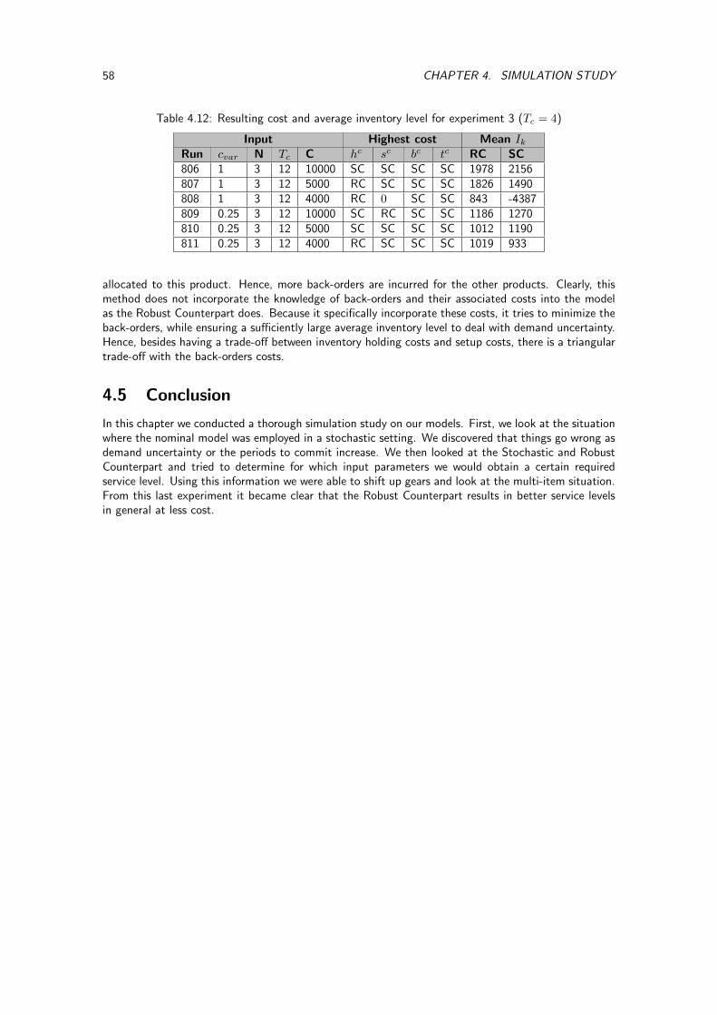
58 CHAPTER 4. SIMULATION STUDY
Table 4.12: Resulting cost and average inventory level for experiment 3 (Tc = 4)
Input Highest cost Mean IkRun cvar N Tc C hc sc bc tc RC SC806 1 3 12 10000 SC SC SC SC 1978 2156807 1 3 12 5000 RC SC SC SC 1826 1490808 1 3 12 4000 RC 0 SC SC 843 -4387809 0.25 3 12 10000 SC RC SC SC 1186 1270810 0.25 3 12 5000 SC SC SC SC 1012 1190811 0.25 3 12 4000 RC SC SC SC 1019 933
allocated to this product. Hence, more back-orders are incurred for the other products. Clearly, thismethod does not incorporate the knowledge of back-orders and their associated costs into the modelas the Robust Counterpart does. Because it specifically incorporate these costs, it tries to minimize theback-orders, while ensuring a sufficiently large average inventory level to deal with demand uncertainty.Hence, besides having a trade-off between inventory holding costs and setup costs, there is a triangulartrade-off with the back-orders costs.
4.5 Conclusion
In this chapter we conducted a thorough simulation study on our models. First, we look at the situationwhere the nominal model was employed in a stochastic setting. We discovered that things go wrong asdemand uncertainty or the periods to commit increase. We then looked at the Stochastic and RobustCounterpart and tried to determine for which input parameters we would obtain a certain requiredservice level. Using this information we were able to shift up gears and look at the multi-item situation.From this last experiment it became clear that the Robust Counterpart results in better service levelsin general at less cost.
Chapter 5
Conclusions and Future Research
5.1 Introduction
In this chapter we will go over the main research findings and make suggestions for future research.First, we will go over the main research question and the related sub questions that we posed in thefirst chapter. In the last three chapters we have been able to answer them. Closely related to theseanswers are the research findings, or implications, that we will discuss in this chapter. We conclude thischapter by discussing possible future research.
For the sake of completeness, we will repeat the main research questions and the related subquestions below,
� What is the relative performance advantage of taking a RO approach to the CLSP over using thenominal model and its Stochastic Counterpart, which is based on the work of Tempelmeier andHilger (2015), in a rolling horizon setting where demand is identically and independently normallydistributed?
and the sub questions,
1. How can we apply the methodologies of RO to production planning problems?
2. How can we derive a Stochastic Counterpart in case we take a stochastic perspective on demanduncertainty?
3. Can we formulate a Robust Counterpart for the nominal CLSP if demand is known to range in aspecified interval?
4. How should we setup an experimental framework and measure the relative performance of themodels?
5. We know that we can influence the realized β-service level in the Stochastic Counterpart by meansof a parameter. However, is the required service level equal to the realized one? If not, how canwe fit the right input to the desired output?
6. How can we influence the realized β-service level in the Robust Counterpart?
7. How much does either of the two models, the Stochastic and Robust Counterpart, perform betterthan the other under different circumstances?
5.2 Main Research Findings
5.2.1 Using Robust Optimization in Production Planning Models
We started our research by explaining the methodologies behind Robust Optimization in 2. Basedon a basic production planning problem we have been able to discuss how this approach deals withuncertainty. Moreover, we have been able to discuss some of the implications of using this method.
59
60 CHAPTER 5. CONCLUSIONS AND FUTURE RESEARCH
Based on results from the work of Bertsimas and Thiele (2006) we have been able to show that theoptimal robust policy for this basic problem in case of interval uncertainty is a base-stock policy. Moreon the implications of this result later. From this chapter it became clear that we could answer thefirst of our sub research questions, Question 1, because we can apply the methodologies of RobustOptimization to production planning models.
In Chapter 3 we again took a Robust Optimization approach, but this time for the Capacitated LotSizing Problem. We started from the nominal problem and showed that it is possible to come up with aRobust Counterpart. So, again we were able to apply the methodologies of Robust Optimization. Thisstrengthens the answer to the Question 1 and answers Question 3.
5.2.2 Deriving a Stochastic Counterpart
So, we derived a Robust and Stochastic Counterpart. The differences between the two is in theway the look at demand uncertainty. The Robust Counterpart looks at uncertainty in a more or lessgeometrical way, because it extends the polyhedron in which it looks for solutions. Contrary, theStochastic Counterpart deals with uncertainty in a stochastic way. This means that it assumes demandto be randomly distributed. In this case, it assumes demand to be identically and independently normallydistributed. However, we saw that it is not straightforward to incorporate this notion of uncertaintyin the nominal CLSP. We had to approximate the functions for the expected inventory level and back-orders.
We started the approximation of the functions for the expected inventory level and back-orders bydefining them in terms of cumulative production quantities. Then we derived an explicit formulation forboth and these formulations allowed us to linearize both. Finally, we were able to come up with the Ap-proximated Stochastic Capacitated Lot Sizing Problem in which these linearizations were incorporated.Hence, we ended up with the Stochastic Counterpart to the nominal problem. This answers Question2, yes we can derive a Stochastic Counterpart for the nominal Capacitated Lot Sizing Problem.
An interesting result followed from preliminary research on this model in our simulation framework.Our model is based predominantly on the work of Tempelmeier and Hilger (2015). But when weimplemented this model we encountered some counter-intuitive behavior. To give a small recapitulationon what goes wrong, the initial model does not properly fill the intervals that are associated withthe parts of the linearized functions. This allows the model to select only those that yield morefavorable values for the expected inventory level and back-order function. It still satisfies the servicelevel constraint, but it no longer results in a sensible production plan. Hence, we showed that the modelof Tempelmeier and Hilger (2015) has its flaws and explained how this could be improved. Of course,our model incorporated these improvements.
5.2.3 Influencing the Realized β-Service Level
Two of our sub research questions, Question 6 and 5 we aimed at investigating if we could influence therealized β-service level. Before we started researching this question in the simulation study, we alreadyknew that the Stochastic Counterpart had a parameter for the required β-service level. We filled insome values to check whether the required service levels correspond to the realized service levels. Wefound a relation between input and output. This enabled us to fit the desired output with the requiredinput. We repeated this for the Robust Counterpart as well and we discovered a relation between theoutputs and the required demand half-widths as inputs. So, yes, we can influence the realized β-servicelevel the way we want it to be.
5.2.4 Relative Performance under Low and High Ratios of Demand to Ca-pacity
We looked at how the models perform if we have three products in our system and if we were totighten capacity. From the last experiment in the previous chapter it became clear that the RobustCounterpart is superior to the Stochastic Counterpart. It makes sense that the service levels drop ascapacity tightens, but clearly, they dropped more in case of the Stochastic Counterpart. As reason forthis phenomenon we gave the strong desire of the Stochastic Counterpart to satisfy the service levelconstraint. This model doesn’t have the trade-off with back-order costs as the Robust Counterpart has.
5.3. FUTURE RESEARCH 61
This gives reason to think that the Robust Counterpart aims at minimizing back-orders costs, inventoryholding cost and setup costs, while the Stochastic Counterpart wants to minimize inventory holdingcosts and setup costs, while satisfying the service levels. However, when the models end up in theposition of significant back-orders the Robust Counterpart acknowledges the importance of reducingthe back-orders for all products, while the Stochastic Counterpart only focusses on achieving the servicelevels (most of the times at cost of the other products).
5.2.5 General Conclusion
In general we may conclude that a Robust Optimization lends itself for the use in production planningmodels, e.g. our single-item problem and the CLSP. Furthermore, we showed how to derive a StochasticCounterpart. By doing so we found out that the model of Tempelmeier and Hilger (2015) has it flaw.Hence, we suggested how to improve this. Furthermore, it is safe to say that the Robust Optimizationapproach leads to a better β-service level at less cost than the Stochastic Counterpart.
We conclude this section by repeating the contributions we made to the field. We showed how totake a Robust Optimization approach to the Capacitated Lot Sizing Problem, we corrected an existingstochastic model and came up with our own Stochastic Counterpart, we simulated our models in arolling horizon setting and gave insight in how to take a Robust Optimization approach.
5.3 Future Research
In this final section of this final chapter we will make recommendations for future research regardingproduction planning and more specific to the Capacitated Lot Sizing Problem. First, we want to saysomething about further use of Robust Optimization. Then we state something about the use of arolling horizon setting in a simulation study. Then we recommend where to go next with regards tostudying a Robust Optimization approach to lot sizing problems.
We touched slightly upon the new developments around Distributionally Robust Optimization inChapter 2 and argued that this might become a third paradigm besides looking at uncertainty from aStochastic or Robust Optimization approach. Though, the word paradigm might be an overstatement asall three methods are closely related. It seems that DRO combines the best of both worlds. It borrowsfrom the notion of probability distributions from the stochastic side, i.e. uncertainty is specified bymoments and other deviation measures. Based on this information a formulation is made using theRobust Optimization methodologies. Although these developments are in its infancy, they are worthkeeping an eye on, because in practice it is hard (and costly) to obtain information about the demanddistribution. Though, the first moments are generally easy to obtain. Hence, DRO sounds promisingwith this respect.
Then with regards to the rolling horizon setting that we took in our simulation study. Previousresearch already suggested to do so, but it is seldom, if not non-existing, encountered in works on theCapacitated Lot Sizing Problem. This is quite remarkable seen the fact that most models employed inpractice run in a rolling horizon. Therefore, in our opinion, performing a simulation study in a rollinghorizon is of utmost importance and intrinsically bound together with proper research. If one doesn’tknow how a model performs in a rolling horizon it is to be expected that nothing can be said aboutits relevance for practice. Hence, we highly recommend future research to run simulations in a rollinghorizon setting.
In our simulation study we have looked at low and high ratios of demand to capacity. While mostworks do not consider high ratios, we explicitly did, because it is important for practice to do so. Thework of Fransoo et al. (1995) pointed out the importance of stable cycle lengths at high ratios ofdemand to capacity. To illustrate this take a look at Figure 5.1. In this figure we have plotted theinventory levels for three products. Clearly, this system is under high pressure, because each setup isfollowed by the respective production of the product. And as production ends, the setup of the nextproduct immediately commences.
In this system it is interesting to see if demand becomes uncertain and we have a higher realizationof demand for a certain product. This situation is illustrated in Figure 5.2. We see an increase in thedemand rate which depletes the inventory for this product much faster. Hence, a setup is required toproduce new products. However, to do so, we have to make a shorter production run for the third
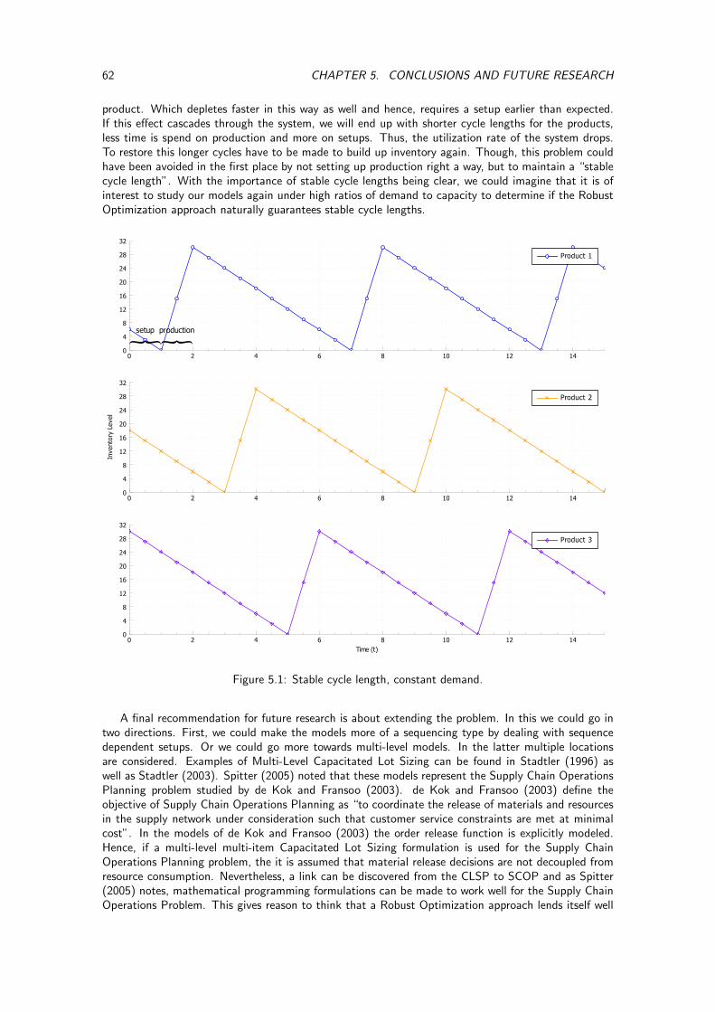
62 CHAPTER 5. CONCLUSIONS AND FUTURE RESEARCH
product. Which depletes faster in this way as well and hence, requires a setup earlier than expected.If this effect cascades through the system, we will end up with shorter cycle lengths for the products,less time is spend on production and more on setups. Thus, the utilization rate of the system drops.To restore this longer cycles have to be made to build up inventory again. Though, this problem couldhave been avoided in the first place by not setting up production right a way, but to maintain a “stablecycle length”. With the importance of stable cycle lengths being clear, we could imagine that it is ofinterest to study our models again under high ratios of demand to capacity to determine if the RobustOptimization approach naturally guarantees stable cycle lengths.
productionsetup
0 2 4 6 8 10 12 14
0
4
8
12
16
20
24
28
32
Product 1
0 2 4 6 8 10 12 14
0
4
8
12
16
20
24
28
32
Invento
ry L
evel
Product 2
0 2 4 6 8 10 12 14
Time (t)
0
4
8
12
16
20
24
28
32
Product 3
Figure 5.1: Stable cycle length, constant demand.
A final recommendation for future research is about extending the problem. In this we could go intwo directions. First, we could make the models more of a sequencing type by dealing with sequencedependent setups. Or we could go more towards multi-level models. In the latter multiple locationsare considered. Examples of Multi-Level Capacitated Lot Sizing can be found in Stadtler (1996) aswell as Stadtler (2003). Spitter (2005) noted that these models represent the Supply Chain OperationsPlanning problem studied by de Kok and Fransoo (2003). de Kok and Fransoo (2003) define theobjective of Supply Chain Operations Planning as “to coordinate the release of materials and resourcesin the supply network under consideration such that customer service constraints are met at minimalcost”. In the models of de Kok and Fransoo (2003) the order release function is explicitly modeled.Hence, if a multi-level multi-item Capacitated Lot Sizing formulation is used for the Supply ChainOperations Planning problem, the it is assumed that material release decisions are not decoupled fromresource consumption. Nevertheless, a link can be discovered from the CLSP to SCOP and as Spitter(2005) notes, mathematical programming formulations can be made to work well for the Supply ChainOperations Problem. This gives reason to think that a Robust Optimization approach lends itself well
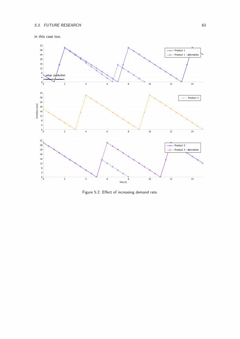
5.3. FUTURE RESEARCH 63
in this case too.
productionsetup
0 2 4 6 8 10 12 14
0
4
8
12
16
20
24
28
32
Product 1
Product 1 - alternative
0 2 4 6 8 10 12 14
0
4
8
12
16
20
24
28
32
Invento
ry L
evel
Product 2
0 2 4 6 8 10 12 14
Time (t)
0
4
8
12
16
20
24
28
32
Product 3
Product 3 - alternative
Figure 5.2: Effect of increasing demand rate.

64 CHAPTER 5. CONCLUSIONS AND FUTURE RESEARCH
Bibliography
Alem, D. and Morabito, R. (2012). Production planning in furniture settings via robust optimization.Computers and Operations Research, 39:139–150.
Allahverdi, A., Gupta, J., and Aldowaisan, T. (1999). A review of scheduling research involving setupconsiderations. Omega, 1999:219–239.
Aouam, T. and Brahimi, N. (2013). Integrated production planning and order acceptance under uncer-tainty: A robust optimization approach. European Journal of Operational Research, 228:504–515.
Belvaux, G. and Wolsey, L. (2001). Modelling practical lot-sizing problems as mixed-integer programs.Management Science, 47(7):993–1007.
Ben-Tal, A., Ghaoui, L. E., and Nemirovski, A. (2009a). Robust Optimization. Princeton UniversityPress, Princeton and Oxford.
Ben-Tal, A., Golany, B., Nemirovski, A., and Vial, J. (2005). Retailer-supplier flexible commitmentcontracts: A robust optimization approach. Manufacturing and Service Operations Management,7(3):248–271.
Ben-Tal, A., Golany, B., and Shtern, S. (2009b). Robust multi-echelon multi-period inventory constrol.European Journal of Operational Research, 199:922–935.
Ben-Tal, A., Goryashko, A., Guslitzer, E., and Nemirovski, A. (2004). Adjustable robust solutions ofuncertain linear programs. Mathematical Programming, Series A, 99:351–376.
Ben-Tal, A. and Nemirovski, A. (1998). Robust convex optimization. Mathematics of OperationsResearch, 23(4):769–805.
Ben-Tal, A. and Nemirovski, A. (1999). Robust solutions of uncertain linear programs. OperationsResearch Letters, 25:1–13.
Ben-Tal, A. and Nemirovski, A. (2000). Robust solutions of linear programming problems contaminatedwith uncertain data. Mathematical Programming, Series A, 88:411–424.
Bertsekas, D. (2001). Dynamic Programming and Optimal Control. Athena Scientific, Belmont.
Bertsimas, D., Brown, D., and Caramanis, C. (2011). Theory and applications of robust optimization.Society for Industrial and Applied Mathematics, 53(3):464–501.
Bertsimas, D. and Georghiou, A. (2015). Design of near optimal decision rules in multistage adaptivemixed-integer optimization. Operations Research, 63(3):610–627.
Bertsimas, D., Iancu, D., and Parrilo, P. (2010). Optimality of affine policies in multistage robustoptimization. Mathematics of Operations Research, 35(2):363–394.
Bertsimas, D. and Sim, M. (2004). The price of robustness. Operations Research, 52(1):35–53.
Bertsimas, D. and Thiele, A. (2006). A robust optimization approach to inventory theory. OperationsResearch, 54(1):150–168.
65
66 BIBLIOGRAPHY
Bertsimas, D. and Tsitsiklis, J. (1997). Introduction to Linear Optimization. Althena Scientific, Nashua,NH.
Bookbinder, J. and Tan, J.-Y. (1988). Strategies for the probabilistic lot-sizing problem with service-level constraints. Management Science, 34(9):1096–1108.
Boyd, S. and Vandenberghe, L. (2004). Convex Optimization. Cambridge University Press, Cambridge.
Clark, A. and Scarf, H. (1960). Optimal policies for a multi-echelon inventory problem. ManagementScience, 6(4):475–490.
Dantzig, G. (1955). Linear programming under uncertainty. Management Science, 1(3/4):197–206.
de Kok, A. and Fransoo, J. (2003). Planning supply chain operations: Definition and comparison ofplanning concepts. In de Kok, A. and Graves, S., editors, Handbooks in Operations Research andManagement Science, volume 11, chapter 12, pages 597–675. Elsevier, Amsterdam, the Netherlands.
Drexl, A. and Kimms, A. (1997). Lot sizing and scheduling - survey and extensions. European Journalof Operational Research, 99:221–235.
Dzielinksi, B., Baker, C., and Manne, A. (1963). Simulation tests of lot size programming. ManagementScience, 9(2):229–258.
Fransoo, J., Sridharan, V., and Bertrand, J. (1995). A hierarchical approach for capacity coordinationin multiple products single-machine production systems with stationary stochastic demand. EuropeanJournal of Operational Research, 86:57–72.
Gorissen, B. and den Hertog, D. (2013). Robust counterparts of inequalities containing sums of maximaof linear functions. European Journal of Operational Research, 227:30–43.
Gorissen, B., Yahnikoglu, I., and den Hertog, D. (2015). A practical guide to robust optimization.Omega, 53:124–137.
Helber, S. and Sahling, F. (2010). A fix-and-optimize approach for the multi-level capacitated lot sizingproblem. International Journal of Production Economics, 123:247–256.
Helber, S., Sahling, F., and Schimmelpfeng, K. (2013). Dynamic capacitated lot sizing with randomdemand and dynamic safety stock. OR Spectrum, 35:75–105.
Jans, R. and Degraeve, Z. (2008). Modeling industrial lot sizing problems: A review. InternationalJournal of Production Research, 46(6):1619–1643.
Karimi, B., Ghomi, S. F., and Wilson, J. (2003). The capacitated lot sizing problem: A review ofmodels and algorithms. Omega, 31:365–378.
Law, A. (2015). Simulation Modeling and Analysis. McGraw-Hill, New York.
Maes, J., McClain, J., and van Wassenhove, L. (1991). Multilevel capacitated lotsizing complexity andlp-based heuristics. European Journal of Operational Research, 53:131–148.
Maes, J. and van Wassenhove, L. (1986). A simple heuristic for the multi item single level capacitatedlotsizing problem. Operations Research Letters, 4(6):265–273.
Manne, A. (1958). Programming of economic lot sizes. Management Science, 4(2):115–135.
Pochet, Y. and Wolsey, L. (2006). Production Planning by Mixed Integer Programming. Springer,Berlin.
Postek, K., Ben-Tal, A., den Hertog, D., and Melenberg, B. (2015). Exact robust counterparts ofambiguous stochastic constraints under mean and dispersion information. CentER Discussion Paper,No. 2015-030.
Postek, K. and den Hertog, D. (2015). Multi-stage adjustable robust mixed-integer optimization viaiterative splitting of the uncertainty set. CentER Discussion Paper, No. 2014-056.
BIBLIOGRAPHY 67
Ross, S. (2010). Introduction to Probability Models. Elsevier, Amsterdam.
Rossi, R., Kilic, N., and Tarim, S. (2015). Piecewise linear approximations for the static-dynamicuncertainty strategy in stochastic lot-sizing. Omega, 50:126–140.
Rossi, R., Tarim, S., Presetwich, S., and Hnich, B. (2014). Piecewise linear lower and upper bounds forthe standard normal first order loss function. Applied Mathematics and Computation, 231:489–502.
Scarf, H., Arrow, K., and Karlin, S. (1958). A min-max solution to an inventory problem. Studies inthe Mathematical Theory of Inventory and Production, pages 201–209.
Silver, E., Pyke, D., and Peterson, R. (1998). Inventory Management and Production Planning andScheduling. John Wiley and Sons, New York.
Sox, C., Jackson, P., Bowman, A., and Muckstadt, J. (1999). A review of the stochastic lot schedulingproblem. International Journal of Production Economics, 62:181–200.
Soyster, A. (1973). Convex programming with set-inclusive constraints and applications to inexactlinear programming. Operations Research, 21(5):1154–1157.
Spitter, J. (2005). Rolling Schedule Approaches for Supply Chain Operations Planning. Beta ResearchSchool for Operations Management and Logistics, Eindhoven University of Technology, Eindhoven.
Stadtler, H. (1996). A lagrangean-based heuristic for dynamic multi-item multi-level constrained lotsizing with setup times. Management Science, 42:738–757.
Stadtler, H. (2003). Multilevel lot sizing with setup times and multiple constrained resources: Internallyrolling schedules with lot sizing windows. Operations Research, 51(3):487–502.
Tempelmeier, H. (2007). On the stochastic uncapacitated dynamic single-item lotsizing problem withservice level constraints. European Journal of Operational Research, 181:184–194.
Tempelmeier, H. (2011). A column generation heuristic for dynamic capacitated lot sizing with randomdemand under a fill rate constraint. Omega, 39:627–633.
Tempelmeier, H. and Herpers, S. (2010). ABCβ - a heuristic for dynamic capacitated lot sizing with ran-dom demand under a fill rate constraint. International Journal of Production Research, 48(17):5181–5193.
Tempelmeier, H. and Hilger, T. (2015). Linear programming models for a stochastic dynamic capaci-tated lot sizing problem. Computers and Operations Research, 59:119–125.
van Houtum, G. (2006). Multiechelon production/inventory systems: Optimal policies, heuristics,and algorithms. In Gray, P., editor, Tutorials in Operations Research, chapter 7, pages 163–199.INFORMS, Hanover, MD.
Wagner, H. and Whitin, T. (1958). Dynamic version of the economic lot size model. ManagementScience, 5:89–96.
Winands, E., Adan, I., and van Houtum, G. (2011). The stochastic economic lot scheduling problem:A survey. European Journal of Operational Research, 210:1–9.
Wolsey, L. (2002). Solving multi-item lot-sizing problems with mip solver using classification andreformulation. Management Science, 48(12):1587–1602.

68 BIBLIOGRAPHY
Summary
In this thesis the Capacitated Lot Sizing Problem under demand uncertainty is considered. This problemdeals with determining a production plan for one machine over a finite horizon for a fixed number ofproducts while being constraint by per period capacity restrictions. Costs are incurred for setting upproduction, holding inventory and incurring back-orders. First a general introduction is given to thethesis. In this introduction we see that the the problem can very well be formulated as a Mixed IntegerLinear Optimization problem. Besides that we gave a motivation for this research. The most importantmotivations for this research are the fact that a thorough study on how lot sizing models behave in arolling horizon is not found in literature and not many models that uncertainty into account. Hence,various researchers have suggested to conduct such a study (see Karimi et al. (2003), Allahverdi et al.(1999) and Jans and Degraeve (2008)). Both are of importance for practice as well, because mostdemand in practice is inherently uncertain and models are most likely to be employed in a rollinghorizon setting.
Two different methods have been taken to deal with uncertainty, i.e. a Robust Optimizationapproach and a Stochastic approach. The methodologies regarding the former originates from the workof Ben-Tal and Nemirovski (1998) and recently gained widespread attention. The reason for this isthat a Robust Optimization doesn’t suffer from the curse of dimensionality as Stochastic Programmingdoes for example, because it deals with uncertainty in a geometrical way. What this means is that thepolyhedron with possible solutions to a mathematical problem is extended. A solution is said to berobust if it resides in this new polyhedron. Another big advantage of this method is that a problemcan be formulated as (Mixed Integer) Linear Optimization problem and stays as such when the RobustCounterpart is derived in most cases.
When dealing with the Stochastic approach we have to take into account that we can no longertalk about inventory level, demand or back-orders. We have to express those in their expected values.However, we can’t deal with these straight away in a Mixed Integer Linear Optimization problem.Therefore, we have determined the Piece-Wise Linear Approximations of the functions for these expectedvalues. These approximations have then be substituted back into the problem to obtain again a linearproblem. Interestingly, while deriving our own model we compared it to the one of Tempelmeier andHilger (2015). We found that their model does not correctly fills the intervals corresponding to thedifferent slopes in the approximation. Their model can be hacked in such a way that only those intervalsare chosen that have the largest slope. This way we can still achieve the requirements of the servicelevel constraint in this model, while incurring less cost. We have tackled this problem and came upwith the so called Stochastic Counterpart.
All models have been compared in an simulated environment in a rolling horizon setting wheredemand is randomly generated from the Normal distribution. First, the nominal problem is investigatedand some interesting property came to light. The results confirm the expectation that the service leveldrops when demand uncertainty increases or when we have to commit more periods. The reason for thisto happen has to do with the trade-off between setup costs and inventory holding costs by the lot sizingdecision. As a consequence of this trade-off the lot size will be larger than the required demand forone period. Hence, our lot size effectively behaves as a safety stock. So, under various circumstanceswe have seen reasonable service levels. Though, a decrease in the realized service level is observed asdemand uncertainty increases or we have to commit more periods.
The realized service level when using the Stochastic Counterpart can be influenced by means of aβ-service level constraint whereas for the Robust Counterpart we can set the back-order cost and thesize of the demand interval. Therefore, we continued with fitting the right parameters to a realizedservice level. This enabled us to asses how these models perform under various circumstances. We
69
70 BIBLIOGRAPHY
observed that the Robust Counterpart delivers more stable service levels at lower cost when capacitydecreases and demand uncertainty gets higher. By careful investigation of the results in this experimentwe found out the reason for this, which we will explain next.
Our primary aim was to achieve a certain service level and secondary to that to keep costs low.The Robust Counterpart yields more steady results, because its keeps the service level among theproducts reasonably stable and it does not drop as dramatically as the Stochastic Counterpart whencapacity tightens and demand uncertainty increases. To understand the reason behind it, recall thatthe Stochastic Counterpart works with a service level in one of its constraints. Then as the system getsunder pressure, it has a strong desire in at least satisfying the service level of one product. All capacityis allocated to this product. Hence, more back-orders are incurred for the other products. Since itdoesn’t take back-order cost into account it has no incentive to reduce the back-orders. Contrary,the Robust Counterpart does take the knowledge of the back-orders and their associated cost intoaccount. Because it specifically incorporates this cost, it tries to minimize the back-orders, while itensures a sufficiently large average inventory level to deal with demand uncertainty. Therefore, besideshaving a trade-off between inventory holding costs and setup costs, it has a triangular trade-off withthe back-orders costs.
In short, we can summarize our contributions as follows. We have taken two approaches to dealwith demand uncertainty and this has led to the Robust and Stochastic Counterpart. The former isbased on the methodologies from Robust Optimization, and such an approach have not yet been taken,while the latter is inspired by the work of, Tempelmeier and Hilger (2015). We have shown that themodel introduced in Tempelmeier and Hilger (2015) does not work correctly. Hence, we have improvedthis model. Thus we contribute two new models to deal with demand uncertainty for the CapacitatedLot Sizing Problem. Furthermore, we have studied how the nominal model, the Robust and StochasticCounterpart perform in a rolling horizon setting under demand uncertainty. Surprisingly, the nominalmodel performs reasonably well in certain circumstances as its lot size effectively behaves like safetystock. In another experiment we have shown that the realized β-service level can be influenced for bothcounterparts. This made them suitable for a comparison under various circumstances. It was foundthat the Robust Counterpart is more stable and results in less cost. Therefore, we have shown that aRobust Optimization approach is not only possible, but leads to better results in general.
Appendices
71

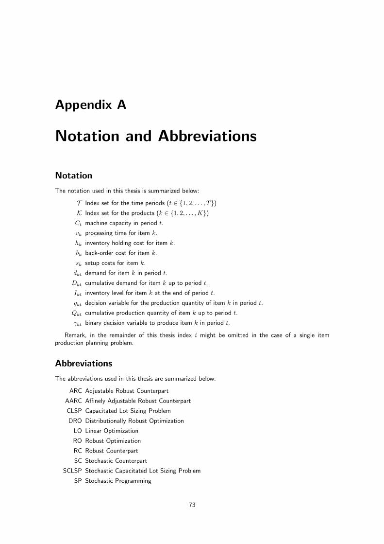
Appendix A
Notation and Abbreviations
Notation
The notation used in this thesis is summarized below:
T Index set for the time periods (t ∈ {1, 2, . . . , T})K Index set for the products (k ∈ {1, 2, . . . ,K})Ct machine capacity in period t.
vk processing time for item k.
hk inventory holding cost for item k.
bk back-order cost for item k.
sk setup costs for item k.
dkt demand for item k in period t.
Dkt cumulative demand for item k up to period t.
Ikt inventory level for item k at the end of period t.
qkt decision variable for the production quantity of item k in period t.
Qkt cumulative production quantity of item k up to period t.
γkt binary decision variable to produce item k in period t.
Remark, in the remainder of this thesis index i might be omitted in the case of a single itemproduction planning problem.
Abbreviations
The abbreviations used in this thesis are summarized below:
ARC Adjustable Robust Counterpart
AARC Affinely Adjustable Robust Counterpart
CLSP Capacitated Lot Sizing Problem
DRO Distributionally Robust Optimization
LO Linear Optimization
RO Robust Optimization
RC Robust Counterpart
SC Stochastic Counterpart
SCLSP Stochastic Capacitated Lot Sizing Problem
SP Stochastic Programming
73

74 APPENDIX A. NOTATION AND ABBREVIATIONS
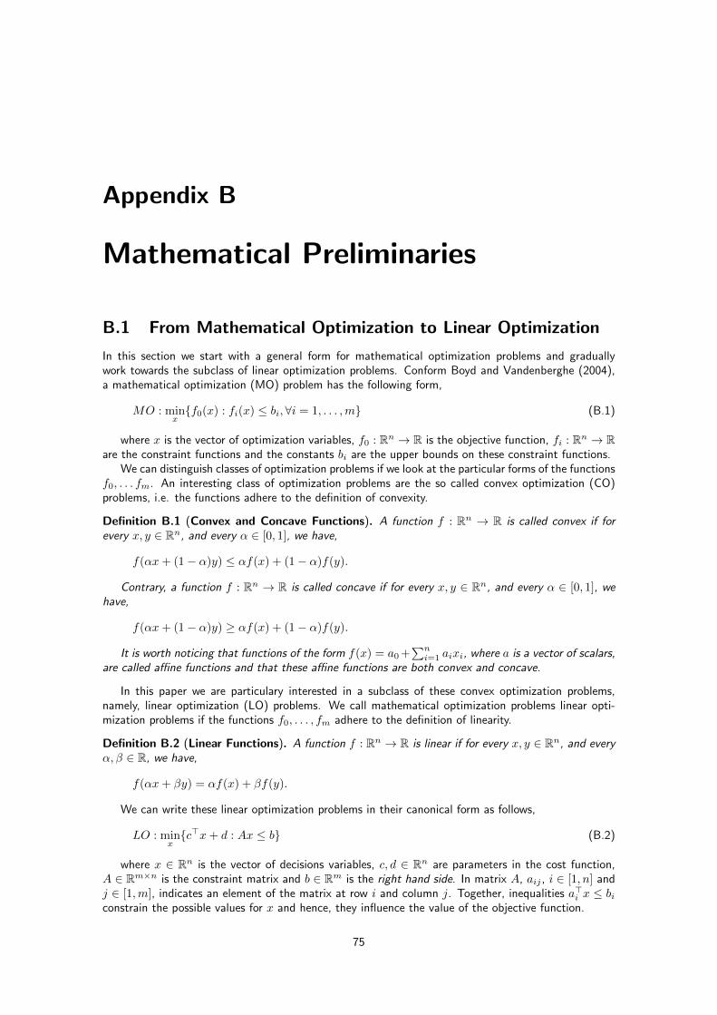
Appendix B
Mathematical Preliminaries
B.1 From Mathematical Optimization to Linear Optimization
In this section we start with a general form for mathematical optimization problems and graduallywork towards the subclass of linear optimization problems. Conform Boyd and Vandenberghe (2004),a mathematical optimization (MO) problem has the following form,
MO : minx{f0(x) : fi(x) ≤ bi,∀i = 1, . . . ,m} (B.1)
where x is the vector of optimization variables, f0 : Rn → R is the objective function, fi : Rn → Rare the constraint functions and the constants bi are the upper bounds on these constraint functions.
We can distinguish classes of optimization problems if we look at the particular forms of the functionsf0, . . . fm. An interesting class of optimization problems are the so called convex optimization (CO)problems, i.e. the functions adhere to the definition of convexity.
Definition B.1 (Convex and Concave Functions). A function f : Rn → R is called convex if forevery x, y ∈ Rn, and every α ∈ [0, 1], we have,
f(αx+ (1− α)y) ≤ αf(x) + (1− α)f(y).
Contrary, a function f : Rn → R is called concave if for every x, y ∈ Rn, and every α ∈ [0, 1], wehave,
f(αx+ (1− α)y) ≥ αf(x) + (1− α)f(y).
It is worth noticing that functions of the form f(x) = a0 +∑ni=1 aixi, where a is a vector of scalars,
are called affine functions and that these affine functions are both convex and concave.
In this paper we are particulary interested in a subclass of these convex optimization problems,namely, linear optimization (LO) problems. We call mathematical optimization problems linear opti-mization problems if the functions f0, . . . , fm adhere to the definition of linearity.
Definition B.2 (Linear Functions). A function f : Rn → R is linear if for every x, y ∈ Rn, and everyα, β ∈ R, we have,
f(αx+ βy) = αf(x) + βf(y).
We can write these linear optimization problems in their canonical form as follows,
LO : minx{c>x+ d : Ax ≤ b} (B.2)
where x ∈ Rn is the vector of decisions variables, c, d ∈ Rn are parameters in the cost function,A ∈ Rm×n is the constraint matrix and b ∈ Rm is the right hand side. In matrix A, aij , i ∈ [1, n] andj ∈ [1,m], indicates an element of the matrix at row i and column j. Together, inequalities a>i x ≤ biconstrain the possible values for x and hence, they influence the value of the objective function.
75
76 APPENDIX B. MATHEMATICAL PRELIMINARIES
B.2 Norms
Definition B.3 (Norms). For p ∈ [1,∞], we define the p-norm ‖.‖p on Rn by the relation,
‖x‖p =
{(∑i |xi|p)1/p, 1 ≤ p <∞
limp→∞ ‖x‖p = maxi{xi}, p =∞.(B.3)
When p, q ∈ [1,∞] and 1p + 1
q = 1, then the norms ‖.‖p and ‖.‖q are conjugates of each other,
‖x‖p = maxy:‖y‖q≤1
|〈x, y〉| (B.4)
In particular, Holder inequality is true, which means that,
|〈x, y〉| ≤ ‖x‖p‖y‖q (B.5)
B.3 Integration
Integration by substitution∫ ψ(b)
ψ(a)
f(x)dx =
∫ b
a
f(ψ(d))ψ′(d)dd (B.6)
Integration by parts∫u(x)v′(x)dx = u(x)v(x)−
∫v(x)u′(x)dx (B.7)
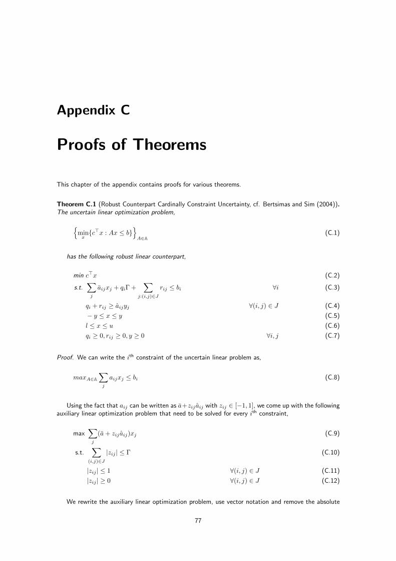
Appendix C
Proofs of Theorems
This chapter of the appendix contains proofs for various theorems.
Theorem C.1 (Robust Counterpart Cardinally Constraint Uncertainty, cf. Bertsimas and Sim (2004)).The uncertain linear optimization problem,
{minx{c>x : Ax ≤ b}
}A∈A
(C.1)
has the following robust linear counterpart,
min c>x (C.2)
s.t.∑j
aijxj + qiΓ +∑
j:(i,j)∈J
rij ≤ bi ∀i (C.3)
qi + rij ≥ aijyj ∀(i, j) ∈ J (C.4)
− y ≤ x ≤ y (C.5)
l ≤ x ≤ u (C.6)
qi ≥ 0, rij ≥ 0, y ≥ 0 ∀i, j (C.7)
Proof. We can write the ith constraint of the uncertain linear problem as,
maxA∈A∑j
aijxj ≤ bi (C.8)
Using the fact that aij can be written as a+zij aij with zij ∈ [−1, 1], we come up with the followingauxiliary linear optimization problem that need to be solved for every ith constraint,
max∑j
(a+ zij aij)xj (C.9)
s.t.∑
(i,j)∈J
|zij | ≤ Γ (C.10)
|zij | ≤ 1 ∀(i, j) ∈ J (C.11)
|zij | ≥ 0 ∀(i, j) ∈ J (C.12)
We rewrite the auxiliary linear optimization problem, use vector notation and remove the absolute
77

78 APPENDIX C. PROOFS OF THEOREMS
values using |zij | = z+ij + z−ij (Bertsimas and Tsitsiklis, 1997, pg. 18),
max(ai1x1 −ai1x1 · · · aijxj −aijxj
)z+i1z−i1...z+ijz−ij
s.t.
1 1 1 1 · · · 1 11 1 0 0 · · · 0 00 0 1 1 · · · 0 0...
......
.... . . 0 0
0 0 0 0 · · · 1 1
z+i1z−i1...z+ijz−ij
≤
Γ11...1
z+ij , z
−ij ≥ 0
The feasible set is non-empty and bounded (z = 0 is a solution), and hence, we can apply strongduality to arrive at the following,
min(Γ 1 1 · · · 1
)qiri1ri2...rij
s.t.
1 1 0 · · · 01 1 0 · · · 01 0 1 · · · 01 0 1 · · · 0...
......
. . ....
1 0 0 · · · 11 0 0 · · · 1
qiri1ri2...rij
≥ai1x1−ai1x1
...aijxj−aijxj
qi ≥ 0, rij ≥ 0
We can introduce the absolute values again, because qi + rij ≥ ai1x1 and qi + rij ≥ −ai1x1(Bertsimas and Tsitsiklis, 1997, pg. 18) and this results in,
min(Γ 1 1 · · · 1
)qiri1ri2...rij
s.t.
1 1 0 · · · 01 0 1 · · · 0...
......
. . ....
1 0 0 · · · 1
qiri1ri2...rij
≥ai1|x1|ai2|x1|
...aij |xj |
qi ≥ 0, rij ≥ 0
We can rewrite the this into the following problem without vector notation,
min qiΓ +∑
j:(i,j)∈J
rij
s.t. qi + rij ≥ aij |xj | ∀j : (i, j) ∈ Jqi ≥ 0, rij ≥ 0 ∀j : (i, j) ∈ J
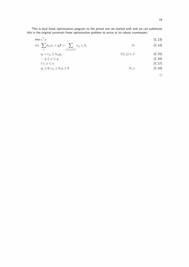
79
This is dual linear optimization program to the primal one we started with and we can substitutethis in the original uncertain linear optimization problem to arrive at its robust counterpart,
min c>x (C.13)
s.t.∑j
aijxj + qiΓ +∑
j:(i,j)∈J
rij ≤ bi ∀i (C.14)
qi + rij ≥ aijyj ∀(i, j) ∈ J (C.15)
− y ≤ x ≤ y (C.16)
l ≤ x ≤ u (C.17)
qi ≥ 0, rij ≥ 0, y ≥ 0 ∀i, j (C.18)