mixed integer programming in production planning with bill...

Submitted tomanuscript (Please, provide the mansucript number!)

Mixed Integer Programming in Production Planningwith Bill-of-materials Structures: Modeling and

AlgorithmsTao Wu∗,†, Leyuan Shi†, Kerem Akartunalı‡

† University of Wisconsin-Madison, Madison, WI 53706, USA, [email protected],

‡ Department of Management Science, University of Strathclyde, Glasgow, G1 1QE, United Kingdom.

[email protected]

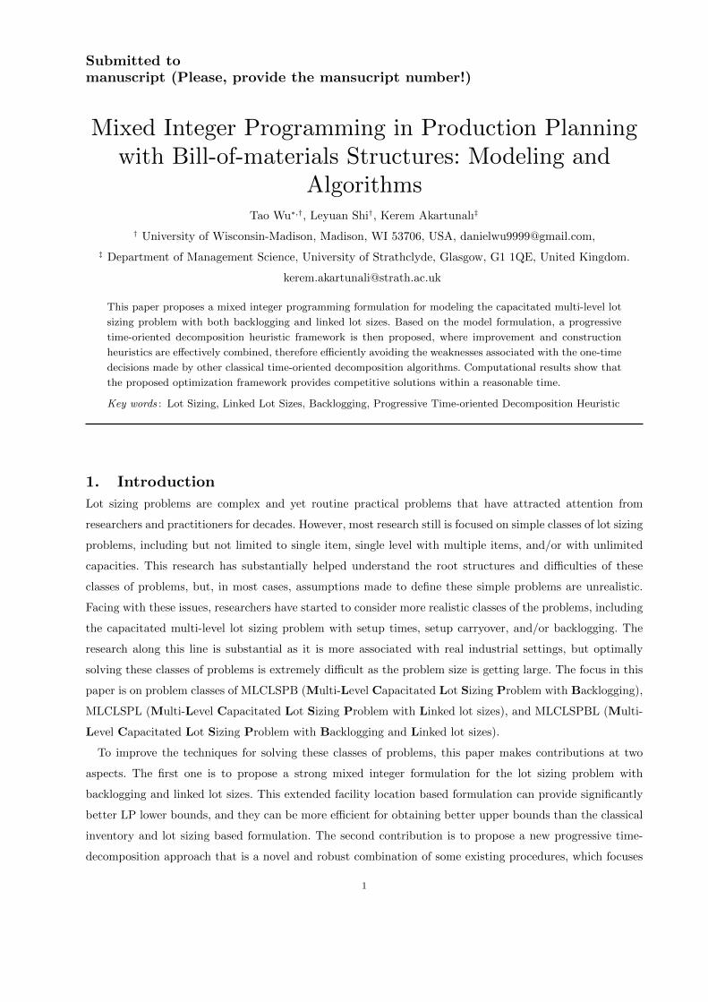
This paper proposes a mixed integer programming formulation for modeling the capacitated multi-level lot

sizing problem with both backlogging and linked lot sizes. Based on the model formulation, a progressive

time-oriented decomposition heuristic framework is then proposed, where improvement and construction

heuristics are effectively combined, therefore efficiently avoiding the weaknesses associated with the one-time

decisions made by other classical time-oriented decomposition algorithms. Computational results show that

the proposed optimization framework provides competitive solutions within a reasonable time.

Key words : Lot Sizing, Linked Lot Sizes, Backlogging, Progressive Time-oriented Decomposition Heuristic

1. Introduction

Lot sizing problems are complex and yet routine practical problems that have attracted attention from

researchers and practitioners for decades. However, most research still is focused on simple classes of lot sizing

problems, including but not limited to single item, single level with multiple items, and/or with unlimited

capacities. This research has substantially helped understand the root structures and difficulties of these

classes of problems, but, in most cases, assumptions made to define these simple problems are unrealistic.

Facing with these issues, researchers have started to consider more realistic classes of the problems, including

the capacitated multi-level lot sizing problem with setup times, setup carryover, and/or backlogging. The

research along this line is substantial as it is more associated with real industrial settings, but optimally

solving these classes of problems is extremely difficult as the problem size is getting large. The focus in this

paper is on problem classes of MLCLSPB (Multi-Level Capacitated Lot Sizing Problem with Backlogging),

MLCLSPL (Multi-Level Capacitated Lot Sizing Problem with Linked lot sizes), and MLCLSPBL (Multi-

Level Capacitated Lot Sizing Problem with Backlogging and Linked lot sizes).

To improve the techniques for solving these classes of problems, this paper makes contributions at two

aspects. The first one is to propose a strong mixed integer formulation for the lot sizing problem with

backlogging and linked lot sizes. This extended facility location based formulation can provide significantly

better LP lower bounds, and they can be more efficient for obtaining better upper bounds than the classical

inventory and lot sizing based formulation. The second contribution is to propose a new progressive time-

decomposition approach that is a novel and robust combination of some existing procedures, which focuses

1

Author: Article Short Title2 Article submitted to ; manuscript no. (Please, provide the mansucript number!)

on the strengths of these methods but avoids their weaknesses. Decomposition is a common technique used in

the literature due to problem complexity in industrial instances. The novelty and difference of our approach

is that many promising subproblems are found in the solution process, increasing the chance of progressively

finding good solutions for the original problem.

To summarize our approach, we first combine the prominent relax-and-fix procedure (SHRF) proposed by

Stadtler (2003) to quickly find an initial feasible solution. This is because the SHRF can efficiently reduce

decomposed problem size as it considers only inventory balance constraints and capacity constraints to

anticipate future capacity bottlenecks in a large number of periods. However, not fully considering capacity

bottlenecks for all periods has a big possibility of deteriorating the solution quality. This is especially true

for the high capacitated lot sizing problem with high seasonality. To avoid the weakness associated with the

SHRF, our solution approach therefore also combines other procedures, including weighted sampling and a

relax-and-fix procedure (AHRF) proposed by Akartunalı and Miller (2010). The weighted sampling procedure

is applied to select a subset of binary setup decision and carryover variables, and then all the variables in this

subset is then fixed to the solution obtained by the SHRF. By doing this way, many promising subproblems

can be found where the size of binary variables is relatively small compared with the original problem. To

solve these subproblems, the AHRF is applied. The advantage of the AHRF over the SHRF is that it always

fully considers the entire planning horizon, ensuring capacity bottlenecks for the periods following the time

windows are well considered. Meanwhile, a quadratically-increasing number of variables associated with the

AHRF is not a big concern anymore as the subproblem with fixed variables is usually relatively small.

The remainder of this paper is organized as follows: Section 2 presents a literature review. Section 3

presents alternative formulations and also makes a brief overview of several time-oriented decomposition

heuristic methods from the literature, with their strengths and weaknesses. Next, Section 4 proposes a

progressive time-oriented decomposition heuristic framework. Section 5 discusses the results of computational

experiments conducted on a number of data sets via a comparison with a commercial solver. Finally, Section

6 concludes and suggests directions for future research.

2. Literature Review

Solution procedures for lot sizing problems vary from exact methods (such as mathematical program-

ming techniques and dynamic programming algorithms) to heuristic methodologies (decomposition-based,

relaxation-based, neighborhood search, to name a few types of heuristics). Exact methodologies are in general

limited to special instances, however they provide us valuable insight. On the other hand, heuristic method-

ologies are crucial for solving problems in the practice, in particular in the industrial settings, although they

might lack of solution quality guarantees. In the following, we present a brief overview of these methods,

covering a few key references as well as recent examples.

The literature on exact methods for lot sizing problems cover a broad range of mathematical programming

techniques. In particular, extended reformulations and valid inequalities have been popular tools. The facility

location reformulation of Krarup and Bilde (1977) and the shortest route reformulation of Eppen and Martin

(1987) have been widely used in the following decades. The family of valid inequalities defined by Barany et al.

Author: Article Short TitleArticle submitted to ; manuscript no. (Please, provide the mansucript number!) 3

(1984) are proven to be useful in practice, in addition to the theoretical fact that, with trivial inequalities,

they define the convex hull of the uncapacitated single-item problem. For various valid inequalities for various

types of lot sizing problems, we refer the interested reader to Pochet and Wolsey (1988), Pochet and Wolsey

(1991), and Miller and Wolsey (2003). Particularly for problems with backlogging, Mathieu (2006) presented

two extended linear programming reformulations of the single-item problem with constant capacities, and

Kucukyavuz and Pochet (2009) recently provided the full definition of the convex hull for the uncapacitated

single item problem. On the other hand, dynamic programming (DP) has been used for some problems,

although DP has been limited to polynomially solvable cases, see e.g. Federgruen and Tzur (1993), Ganas

and Papachristos (2005) and Song and Chan (2005) proposing DP algorithms for various single-item lot

sizing problem with backlogging.

The majority of the heuristic methods presented in the literature for lot sizing problems are construction

heuristics, i.e., heuristics that generate a feasible solution from scratch, and we will provide an overview of

these in the following. However, it is also important to note that there are some good examples of improvement

heuristics, i.e., methods that build up on a given initial solution. One recent example is the fix-and-optimize

heuristic of Sahling et al. (2009) proposed for solving the capacitated multi-level lot sizing problem with

general product structures and with setup-carryover. We refer the interested reader also to ? and ? for other

recent examples.

Decomposition based heuristics include time-oriented or item-oriented decomposition based heuristics. For

example, Kim et al. (2010) proposed a solution approach for lot sizing problems by dividing a time period into

a number of micro time periods, in which a time horizon is treated as a continuum, instead of as a collection

of discrete time periods. Belvaux and Wolsey (2000), Suerie and Stadtler (2003), Federgruen et al. (2007),

and Akartunalı and Miller (2009) are successful examples of time-oriented decomposition approaches. ? and

? used relax-and-fix heuristics in industrial settings for combinations of lot sizing and scheduling problems.

Relaxation based heuristics usually employ Lagrangean relaxation. Millar and Yang (1994) proposed two

Lagrangian decomposition and relaxation algorithms for solving the capacitated single-level multi-item lot

sizing problem with backlogging. Sox and Gao (1999) proposed a Lagrangian decomposition heuristic for

solving large capacitated multi-item lot sizing problems without setup times, but with setup-carryover.

Briskorn (2006) later claimed that the Lagrangian heuristic proposed by Sox and Gao (1999) can not guar-

antee an optimal solution when solving Lagrangian relaxation subproblems, and they revised the heuristic to

ensure the optimality. Tempelmeier and Buschkuhl (2009) proposed a Lagrangean heuristic for the dynamic

capacitated multi-level lot sizing problem with linked lot sizes.

Neighborhood search heuristic is another group of heuristics. The LP-based heuristic of Kuik et al. (1993)

was well compared to the performance of other approaches based on simulated annealing and tabu search

techniques. Tabu search was extensively employed by various researchers, see e.g. Gopalakrishnan et al.

(2001) (problems with set-up carryover), Hung et al. (2003) (problems with multiple items and machines,

setup times and costs), Karimi et al. (2006) (capacitated problem with setup-carryover) and Almada-Lobo

and James (2010) (incorporating with a neighborhood search heuristic to handle sequence-dependent setup

times and costs).


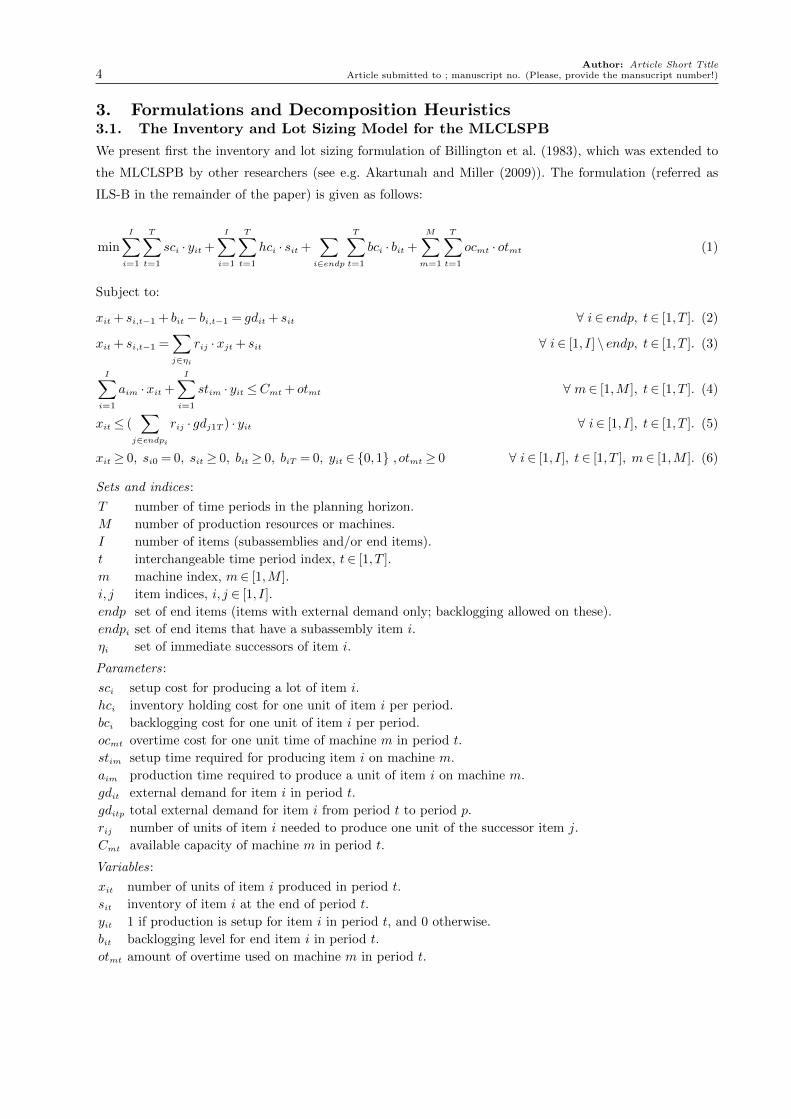
3. Formulations and Decomposition Heuristics3.1. The Inventory and Lot Sizing Model for the MLCLSPB

We present first the inventory and lot sizing formulation of Billington et al. (1983), which was extended to

the MLCLSPB by other researchers (see e.g. Akartunalı and Miller (2009)). The formulation (referred as

ILS-B in the remainder of the paper) is given as follows:

min

I∑i=1

T∑t=1

sci · yit +

I∑i=1

T∑t=1

hci · sit +∑i∈endp

T∑t=1

bci · bit +

M∑m=1

T∑t=1

ocmt · otmt (1)

Subject to:

xit + si,t−1 + bit− bi,t−1 = gdit + sit ∀ i∈ endp, t∈ [1, T ]. (2)

xit + si,t−1 =∑j∈ηi

rij ·xjt + sit ∀ i∈ [1, I] \ endp, t∈ [1, T ]. (3)

I∑i=1

aim ·xit +

I∑i=1

stim · yit ≤Cmt + otmt ∀ m∈ [1,M ], t∈ [1, T ]. (4)

xit ≤ (∑

j∈endpi

rij · gdj1T ) · yit ∀ i∈ [1, I], t∈ [1, T ]. (5)

xit ≥ 0, si0 = 0, sit ≥ 0, bit ≥ 0, biT = 0, yit ∈ {0,1} , otmt ≥ 0 ∀ i∈ [1, I], t∈ [1, T ], m∈ [1,M ]. (6)

Sets and indices:

T number of time periods in the planning horizon.

M number of production resources or machines.

I number of items (subassemblies and/or end items).

t interchangeable time period index, t∈ [1, T ].

m machine index, m∈ [1,M ].

i, j item indices, i, j ∈ [1, I].

endp set of end items (items with external demand only; backlogging allowed on these).

endpi set of end items that have a subassembly item i.

ηi set of immediate successors of item i.

Parameters:

sci setup cost for producing a lot of item i.

hci inventory holding cost for one unit of item i per period.

bci backlogging cost for one unit of item i per period.

ocmt overtime cost for one unit time of machine m in period t.

stim setup time required for producing item i on machine m.

aim production time required to produce a unit of item i on machine m.

gdit external demand for item i in period t.

gditp total external demand for item i from period t to period p.

rij number of units of item i needed to produce one unit of the successor item j.

Cmt available capacity of machine m in period t.

Variables:

xit number of units of item i produced in period t.

sit inventory of item i at the end of period t.

yit 1 if production is setup for item i in period t, and 0 otherwise.

bit backlogging level for end item i in period t.

otmt amount of overtime used on machine m in period t.


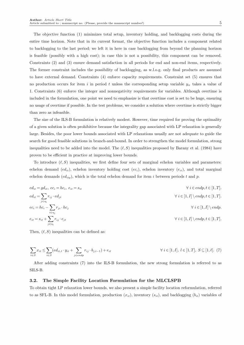
The objective function (1) minimizes total setup, inventory holding, and backlogging costs during the

entire time horizon. Note that in its current format, the objective function includes a component related

to backlogging to the last period; we left it in here in case backlogging from beyond the planning horizon

is feasible (possibly with a high cost); in case this is not a possibility, this component can be removed.

Constraints (2) and (3) ensure demand satisfaction in all periods for end and non-end items, respectively.

The former constraint includes the possibility of backlogging, as w.l.o.g. only final products are assumed

to have external demand. Constraints (4) enforce capacity requirements. Constraint set (5) ensures that

no production occurs for item i in period t unless the corresponding setup variable yit takes a value of

1. Constraints (6) enforce the integer and nonnegativity requirements for variables. Although overtime is

included in the formulation, one point we need to emphasize is that overtime cost is set to be huge, ensuring

no usage of overtime if possible. In the test problems, we consider a solution where overtime is strictly bigger

than zero as infeasible.

The size of the ILS-B formulation is relatively modest. However, time required for proving the optimality

of a given solution is often prohibitive because the integrality gap associated with LP relaxation is generally

large. Besides, the poor lower bounds associated with LP relaxations usually are not adequate to guide the

search for good feasible solutions in branch-and-bound. In order to strengthen the model formulation, strong

inequalities need to be added into the model. The (`,S) inequalities proposed by Barany et al. (1984) have

proven to be efficient in practice at improving lower bounds.

To introduce (`,S) inequalities, we first define four sets of marginal echelon variables and parameters:

echelon demand (edit), echelon inventory holding cost (eci), echelon inventory (eit), and total marginal

echelon demands (editp), which is the total echelon demand for item i between periods t and p.

edit = gdit, eci = hci, eit = sit ∀ i∈ endp, t∈ [1, T ].

edit =∑j∈ηi

rij · edjt ∀ i∈ [1, I] \ endp, t∈ [1, T ].

eci = hci−∑i∈ηj

rji ·hcj ∀ i∈ [1, I] \ endp.

eit = sit +∑j∈ηi

rij · ejt ∀ i∈ [1, I] \ endp, t∈ [1, T ].

Then, (`,S) inequalities can be defined as:

∑t∈S

xit ≤∑t∈S

(edit,` · yit +∑

j∈endp

rij · bj,t−1) + ei` ∀ i∈ [1, I], l ∈ [1, T ], S ⊆ [1, `]. (7)

After adding constraints (7) into the ILS-B formulation, the new strong formulation is referred to as

SILS-B.

3.2. The Simple Facility Location Formulation for the MLCLSPB

To obtain tight LP relaxation lower bounds, we also present a simple facility location reformulation, referred

to as SFL-B. In this model formulation, production (xit), inventory (sit), and backlogging (bit) variables of


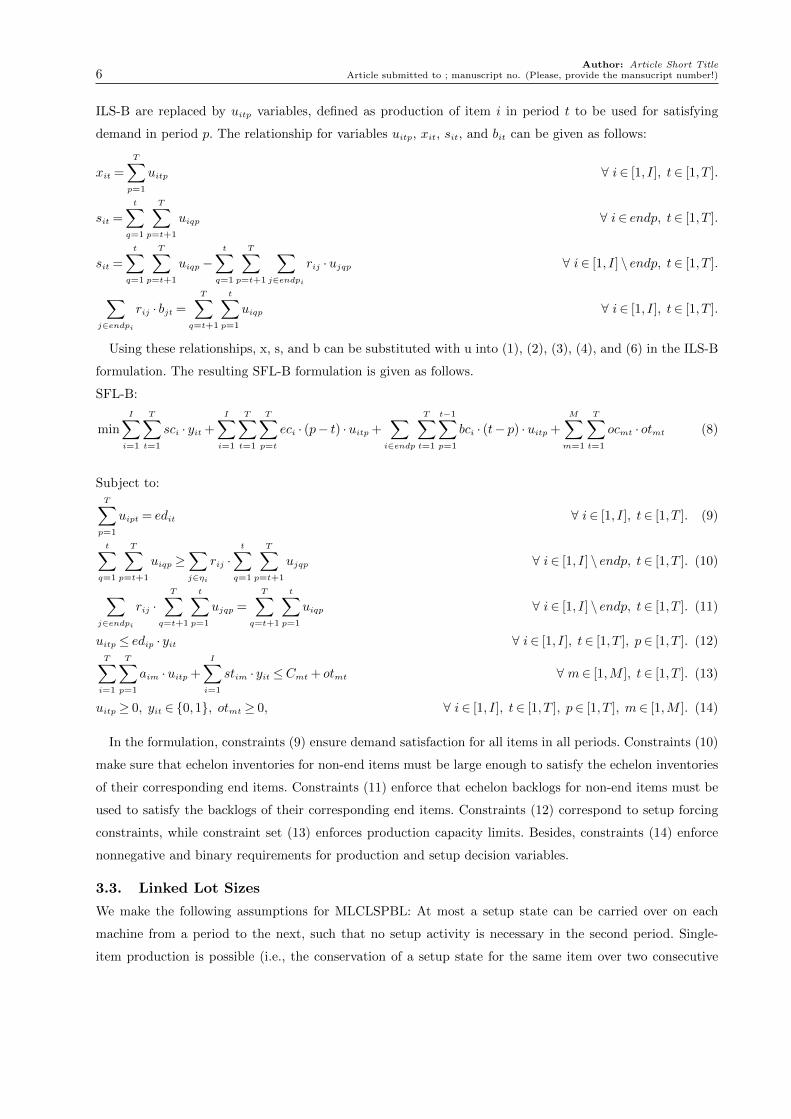
ILS-B are replaced by uitp variables, defined as production of item i in period t to be used for satisfying

demand in period p. The relationship for variables uitp, xit, sit, and bit can be given as follows:

xit =

T∑p=1

uitp ∀ i∈ [1, I], t∈ [1, T ].

sit =

t∑q=1

T∑p=t+1

uiqp ∀ i∈ endp, t∈ [1, T ].

sit =

t∑q=1

T∑p=t+1

uiqp−t∑

q=1

T∑p=t+1

∑j∈endpi

rij ·ujqp ∀ i∈ [1, I] \ endp, t∈ [1, T ].

∑j∈endpi

rij · bjt =

T∑q=t+1

t∑p=1

uiqp ∀ i∈ [1, I], t∈ [1, T ].

Using these relationships, x, s, and b can be substituted with u into (1), (2), (3), (4), and (6) in the ILS-B

formulation. The resulting SFL-B formulation is given as follows.

SFL-B:

min

I∑i=1

T∑t=1

sci · yit +

I∑i=1

T∑t=1

T∑p=t

eci · (p− t) ·uitp +∑i∈endp

T∑t=1

t−1∑p=1

bci · (t− p) ·uitp +

M∑m=1

T∑t=1

ocmt · otmt (8)

Subject to:T∑p=1

uipt = edit ∀ i∈ [1, I], t∈ [1, T ]. (9)

t∑q=1

T∑p=t+1

uiqp ≥∑j∈ηi

rij ·t∑

q=1

T∑p=t+1

ujqp ∀ i∈ [1, I] \ endp, t∈ [1, T ]. (10)

∑j∈endpi

rij ·T∑

q=t+1

t∑p=1

ujqp =

T∑q=t+1

t∑p=1

uiqp ∀ i∈ [1, I] \ endp, t∈ [1, T ]. (11)

uitp ≤ edip · yit ∀ i∈ [1, I], t∈ [1, T ], p∈ [1, T ]. (12)T∑i=1

T∑p=1

aim ·uitp +

I∑i=1

stim · yit ≤Cmt + otmt ∀ m∈ [1,M ], t∈ [1, T ]. (13)

uitp ≥ 0, yit ∈ {0,1}, otmt ≥ 0, ∀ i∈ [1, I], t∈ [1, T ], p∈ [1, T ], m∈ [1,M ]. (14)

In the formulation, constraints (9) ensure demand satisfaction for all items in all periods. Constraints (10)

make sure that echelon inventories for non-end items must be large enough to satisfy the echelon inventories

of their corresponding end items. Constraints (11) enforce that echelon backlogs for non-end items must be

used to satisfy the backlogs of their corresponding end items. Constraints (12) correspond to setup forcing

constraints, while constraint set (13) enforces production capacity limits. Besides, constraints (14) enforce

nonnegative and binary requirements for production and setup decision variables.

3.3. Linked Lot Sizes

We make the following assumptions for MLCLSPBL: At most a setup state can be carried over on each

machine from a period to the next, such that no setup activity is necessary in the second period. Single-

item production is possible (i.e., the conservation of a setup state for the same item over two consecutive


bucket boundaries). A setup state is not lost if there is no production on a machine within a period. These

assumptions are realistic and common, see e.g. Suerie and Stadtler (2003).

To include setup-carryover into the model formulation, two new sets of variables have to be introduced.

The first set is lkit, the binary setup-carryover decision variable vector. lkit is 1 if a setup state for item i is

carried over from period t− 1 to period t, and 0 otherwise. The second set of variables is zmt, which become

1 if the production on resource m in period t is limited to at most an item for which no setup has to be

performed because the setup state for this specific item is linked to both the preceding and next periods,

and 0 otherwise. We also define Rm to be the subset of items that are processed on resource m.

To formulate the MLCLSPBL, constraints (15) - (19) have to be added:∑i∈Rm

lkit ≤ 1 ∀ m∈ [1,M ], t∈ [2, T ]. (15)

lkit ≤ yi(t−1) + lki(t−1) ∀ i∈ [1, I], t∈ [2, T ]. (16)

lki(t+1) + lkit ≤ 1 + zmt ∀ i∈Rm, t∈ [1, T − 1], m∈ [1,M ]. (17)

yit + zmt ≤ 1 ∀ i∈Rm, t∈ [1, T ], m∈ [1,M ]. (18)

lkit ∈ {0,1}, zmt ∈ {0,1} ∀ i∈ [1, I], t∈ [1, T ], m∈ [1,M ]. (19)

uitp ≤ edip · (yit + lkit) ∀ i∈ [1, I], t∈ [1, T ], p∈ [t, T ]. (20)

In addition, setup constraints (12) within SFL-B have to be substituted by constraints (20). The new

formulation for the MLCLSPBL is referred to as SFL-BL. In the formulation, constraints (15) guarantee

that at most one setup state can be preserved from one period to the next on each machine. Constraints

(16) make sure that a setup can be carried over to period t only if either item i is setup in period t− 1 or

the setup state already has been carried over from period t− 2 to period t− 1. Constraints (17) ensure zmt

be equal to 1 if a setup state is preserved both over period t− 1 to period t and over period t to period

t+ 1. Constraints (18) enforce that a performance of a setup and a preservation of a setup status can not

happen simultaneously for a machine within a period. Constraints (19) enforce integrality and nonnegativity

requirements for setup linkage variables. Constraints (20) ensure that the total amount of production is less

than a sufficiently large value and that either a setup or a setup-carryover is performed in period t for item

i if any demand is satisfied using the corresponding production.

Similarly, to formulate MLCLSPL, constraints (15) - (19) have to be added to the classical formulation for

the multi-level capacitated lot sizing problem. We omit the details here as it is trivial to switch the ILS-B

and SFL-B formulations to model the multi-level capacitated lot sizing problem with linked lot sizes without

consideration of backlogging.

3.4. Time-Oriented Decomposition Heuristics

Time-oriented decomposition heuristics, including relax-and-fix, are efficiently used for lot sizing problems.

We discuss here three previously developed heuristics that use relax-and-fix.

Belvaux and Wolsey (2000) proposed the first systematic production planning tool (bc-prod) that uses

relax-and-fix, a specialized branch-and-cut system for lot sizing problems. Bc-prod first generates cutting


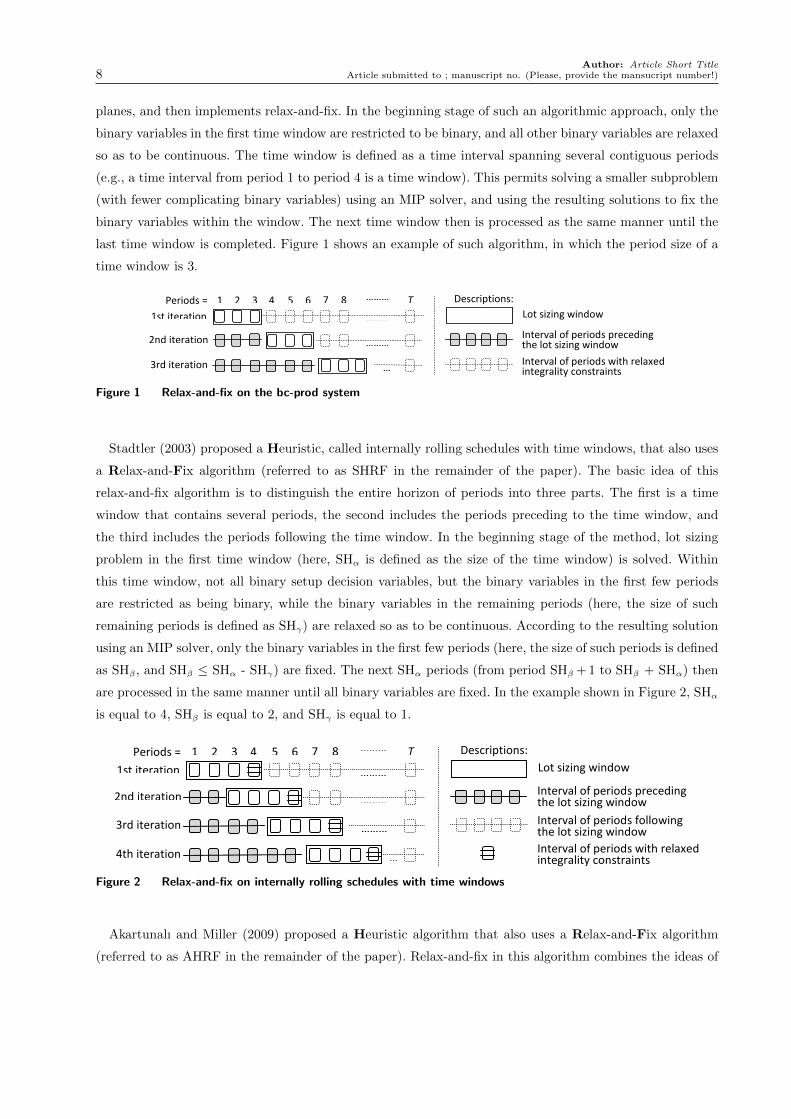
planes, and then implements relax-and-fix. In the beginning stage of such an algorithmic approach, only the

binary variables in the first time window are restricted to be binary, and all other binary variables are relaxed

so as to be continuous. The time window is defined as a time interval spanning several contiguous periods

(e.g., a time interval from period 1 to period 4 is a time window). This permits solving a smaller subproblem

(with fewer complicating binary variables) using an MIP solver, and using the resulting solutions to fix the

binary variables within the window. The next time window then is processed as the same manner until the

last time window is completed. Figure 1 shows an example of such algorithm, in which the period size of a

time window is 3.

Descriptions: Periods = 1

3rd iteration

2nd iteration

1st iteration ………

………

………

2 3 4 5 6 7 8 T ……… Lot sizing window

Interval of periods preceding the lot sizing window Interval of periods with relaxed integrality constraints

Figure 1 Relax-and-fix on the bc-prod system

Stadtler (2003) proposed a Heuristic, called internally rolling schedules with time windows, that also uses

a Relax-and-Fix algorithm (referred to as SHRF in the remainder of the paper). The basic idea of this

relax-and-fix algorithm is to distinguish the entire horizon of periods into three parts. The first is a time

window that contains several periods, the second includes the periods preceding to the time window, and

the third includes the periods following the time window. In the beginning stage of the method, lot sizing

problem in the first time window (here, SHα is defined as the size of the time window) is solved. Within

this time window, not all binary setup decision variables, but the binary variables in the first few periods

are restricted as being binary, while the binary variables in the remaining periods (here, the size of such

remaining periods is defined as SHγ) are relaxed so as to be continuous. According to the resulting solution

using an MIP solver, only the binary variables in the first few periods (here, the size of such periods is defined

as SHβ, and SHβ ≤ SHα - SHγ) are fixed. The next SHα periods (from period SHβ + 1 to SHβ + SHα) then

are processed in the same manner until all binary variables are fixed. In the example shown in Figure 2, SHα

is equal to 4, SHβ is equal to 2, and SHγ is equal to 1.

………


3rd iteration

2nd iteration


………

………

2 3 4 5 6 7 8 T ……… Lot sizing window

Interval of periods preceding the lot sizing window Interval of periods following the lot sizing window

4th iteration Interval of periods with relaxed integrality constraints

Figure 2 Relax-and-fix on internally rolling schedules with time windows

Akartunalı and Miller (2009) proposed a Heuristic algorithm that also uses a Relax-and-Fix algorithm

(referred to as AHRF in the remainder of the paper). Relax-and-fix in this algorithm combines the ideas of


two previously mentioned methods. Specifically, it emphasizes the entire time horizon by relaxing all binary

decision variables in the periods following the time window as bc-prod does, but it does not fix all binary

decision variables in the time window after one iteration as SHRF does. One example of AHRF is shown in

Figure 3, in which the window size (here, we define the window size as AHα) is 4, and the size of overlapping

periods (here, the size of overlapping periods is defined as AHβ) is 2.


3rd iteration

2nd iteration


………

………

2 3 4 5 6 7 8 T ……… Interval of time with binary setup variables

Interval of time with fixed setup variables

Interval of time with relaxed setup variables

Figure 3 Relax-and-fix on the Akartunalı and Miller (2009)’s heuristic algorithm

These three methods are efficient at solving capacitated lot sizing problems. The advantage of bc-prod and

AHRF is that the entire planning horizon is always fully considered, ensuring capacity bottlenecks for the

periods following the time windows are well considered. SHRF treats the periods following a time window

in a different way. Instead of relaxing all binary variables in these periods, as bc-prod and AHRF do, SHRF

considers only inventory balance constraints and capacity constraints (i.e. it does not consider setup times)

included in the model formulation to anticipate future capacity bottlenecks. The reason for this approach is

that a tight extended model is just formulated inside the lot sizing window, not for the entire time horizon.

Consequently, the drawback of an inflated matrix caused by the extended variables can be avoided.

The disadvantage of bc-prod and AHRF is that, under a limited solution time, solution qualities might be

not as good when the problem size gets larger. This issue has a low impact on solution qualities obtained by

SHRF. However, not fully considering capacity bottlenecks for the periods following the time window might

deteriorate the solution quality. This is especially true for the high capacitated lot sizing problem with high

seasonality, for which unexpected effects caused by previously-made bad decisions in the early iteration(s)

could be growing with time windows rolling, resulting in the final solution being bad. The progressive time-

oriented decomposition framework proposed in this paper is designed in an attempt to reduce the risk of

unfavorable setup decisions being made on relax-and-fix, and to utilize the advantages of both AHRF and

SHRF.

4. The Progressive Time-Oriented Decomposition HeuristicFramework

The Progressive Time-oriented decomposition Heuristic (PTH) framework is designed to systematically fix

binary decision variables in order to improve solution quality. Rather than solving initial problems that are

difficult to solve, the framework focuses on solving promising subproblems, where some binary variables are

fixed. Several techniques are incorporated into the framework, including LP-fix, SHRF, AHRF, and weighted

sampling. In this paper, three different scenarios of the framework are proposed. The first scenario combines


the techniques of SHRF and AHRF, the second scenario incorporates the LP-fix technique as well, and the

third scenario incorporates all the techniques.

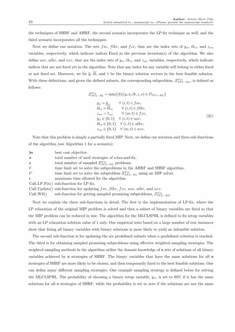
Next we define our notation. The sets fsv, flkv, and fzv, that are the index sets of yit, lkit, and zmt

variables, respectively, which indicate indices f ixed in the previous iteration(s) of the algorithm. We also

define usv, ulkv, and uzv, that are the index sets of yit, lkit, and zmt variables, respectively, which indicate

indices that are not fixed yet in the algorithm. Note that any index for any variable will belong to either fixed

or not fixed set. Moreover, we let y, lk, and z be the binary solution vectors in the best feasible solution.

With these definitions, and given the defined subsets, the corresponding subproblem, ZFixSFL−BL, is defined as

follows:

ZFixSFL−BL = min{(8)|(y,u, lk, z, o)∈ PSFL−BL}

yit = yit ∀ (i, t)∈ fsv,lkit = lkit ∀ (i, t)∈ flkv,zmt = zmt ∀ (m,t)∈ fzv,yit ∈ {0,1} ∀ (i, t)∈ usv,lkit ∈ {0,1} ∀ (i, t)∈ ulkv,zmt ∈ {0,1} ∀ (m,t)∈ uzv.

(21)

Note that this problem is simply a partially fixed MIP. Next, we define our notation and three sub-functions

of the algorithm (see Algorithm 1 for a scenario):

bs best cost objective.

n total number of used strategies of relax-and-fix.

s total number of sampled ZFixSFL−BL problems.

t′ time limit set to solve the subproblems in the AHRF and SHRF algorithm.

t′′ time limit set to solve the subproblem ZFixSFL−BL using an MIP solver.

t maximum time allowed for the algorithm.

Call LP Fix() sub-function for LP-fix.

Call Update() sub-function for updating fsv, flkv, fzv, usv, ulkv, and uzv.

Call WS() sub-function for getting sampled promising subproblems, ZFixSFL−BL.

Next we explain the three sub-functions in detail. The first is the implementation of LP-fix, where the

LP relaxation of the original MIP problem is solved and then a subset of binary variables are fixed so that

the MIP problem can be reduced in size. The algorithm for the MLCLSPBL is defined to fix setup variables

with an LP relaxation solution value of 1 only. Our empirical tests based on a large number of test instances

show that fixing all binary variables with binary solutions is more likely to yield an infeasible solution.

The second sub-function is for updating the six predefined subsets when a predefined criterion is reached.

The third is for obtaining sampled promising subproblems using effective weighted sampling strategies. The

weighted sampling methods in the algorithm utilize the domain knowledge of n sets of solutions of all binary

variables achieved by n strategies of SHRF. The binary variables that have the same solutions for all n

strategies of SHRF are more likely to be chosen, and then temporarily fixed to the best feasible solutions. One

can define many different sampling strategies. One example sampling strategy is defined below for solving

the MLCLSPBL. The probability of choosing a binary setup variable, yit, is set to 80% if it has the same

solutions for all n strategies of SHRF, while the probability is set to zero if the solutions are not the same


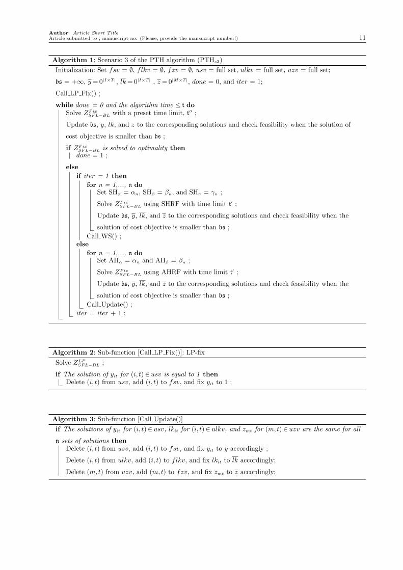
Algorithm 1: Scenario 3 of the PTH algorithm (PTHs3)

Initialization: Set fsv = ∅, flkv = ∅, fzv = ∅, usv = full set, ulkv = full set, uzv = full set;

bs = +∞, y= 0|I×T |, lk= 0|I×T | , z = 0|M×T |, done = 0, and iter = 1;

Call LP Fix() ;

while done = 0 and the algorithm time ≤ t doSolve ZFixSFL−BL with a preset time limit, t′′ ;

Update bs, y, lk, and z to the corresponding solutions and check feasibility when the solution of

cost objective is smaller than bs ;

if ZFixSFL−BL is solved to optimality thendone = 1 ;

else

if iter = 1 then

for n = 1,..., n doSet SHα = αn, SHβ = βn, and SHγ = γn ;

Solve ZFixSFL−BL using SHRF with time limit t′ ;

Update bs, y, lk, and z to the corresponding solutions and check feasibility when the

solution of cost objective is smaller than bs ;

Call WS() ;else

for n = 1,..., n doSet AHα = αn and AHβ = βn ;

Solve ZFixSFL−BL using AHRF with time limit t′ ;

Update bs, y, lk, and z to the corresponding solutions and check feasibility when the

solution of cost objective is smaller than bs ;

Call Update() ;

iter = iter + 1 ;

Algorithm 2: Sub-function [Call LP Fix()]: LP-fix

Solve ZLPSFL−BL ;

if The solution of yit for (i, t)∈ usv is equal to 1 thenDelete (i, t) from usv, add (i, t) to fsv, and fix yit to 1 ;

Algorithm 3: Sub-function [Call Update()]

if The solutions of yit for (i, t)∈ usv, lkit for (i, t)∈ ulkv, and zmt for (m,t)∈ uzv are the same for all

n sets of solutions thenDelete (i, t) from usv, add (i, t) to fsv, and fix yit to y accordingly ;

Delete (i, t) from ulkv, add (i, t) to flkv, and fix lkit to lk accordingly;

Delete (m,t) from uzv, add (m,t) to fzv, and fix zmt to z accordingly;


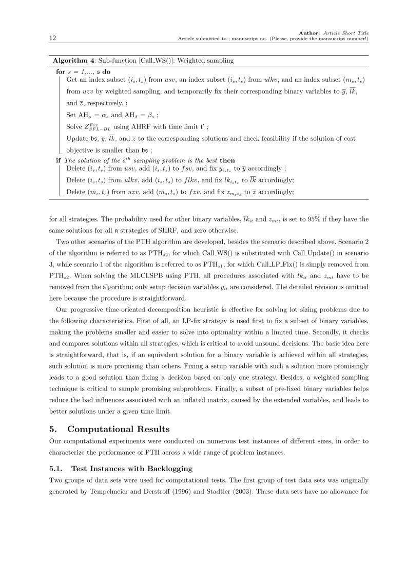
Algorithm 4: Sub-function [Call WS()]: Weighted sampling

for s = 1,..., s doGet an index subset (is, ts) from usv, an index subset (is, ts) from ulkv, and an index subset (ms, ts)

from uzv by weighted sampling, and temporarily fix their corresponding binary variables to y, lk,

and z, respectively. ;

Set AHα = αs and AHβ = βs ;

Solve ZFixSFL−BL using AHRF with time limit t′ ;

Update bs, y, lk, and z to the corresponding solutions and check feasibility if the solution of cost

objective is smaller than bs ;

if The solution of the sth sampling problem is the best thenDelete (is, ts) from usv, add (is, ts) to fsv, and fix yists to y accordingly ;

Delete (is, ts) from ulkv, add (is, ts) to flkv, and fix lkists to lk accordingly;

Delete (ms, ts) from uzv, add (ms, ts) to fzv, and fix zmsts to z accordingly;

for all strategies. The probability used for other binary variables, lkit and zmt, is set to 95% if they have the

same solutions for all n strategies of SHRF, and zero otherwise.

Two other scenarios of the PTH algorithm are developed, besides the scenario described above. Scenario 2

of the algorithm is referred to as PTHs2, for which Call WS() is substituted with Call Update() in scenario

3, while scenario 1 of the algorithm is referred to as PTHs1, for which Call LP Fix() is simply removed from

PTHs2. When solving the MLCLSPB using PTH, all procedures associated with lkit and zmt have to be

removed from the algorithm; only setup decision variables yit are considered. The detailed revision is omitted

here because the procedure is straightforward.

Our progressive time-oriented decomposition heuristic is effective for solving lot sizing problems due to

the following characteristics. First of all, an LP-fix strategy is used first to fix a subset of binary variables,

making the problems smaller and easier to solve into optimality within a limited time. Secondly, it checks

and compares solutions within all strategies, which is critical to avoid unsound decisions. The basic idea here

is straightforward, that is, if an equivalent solution for a binary variable is achieved within all strategies,

such solution is more promising than others. Fixing a setup variable with such a solution more promisingly

leads to a good solution than fixing a decision based on only one strategy. Besides, a weighted sampling

technique is critical to sample promising subproblems. Finally, a subset of pre-fixed binary variables helps

reduce the bad influences associated with an inflated matrix, caused by the extended variables, and leads to

better solutions under a given time limit.

5. Computational Results

Our computational experiments were conducted on numerous test instances of different sizes, in order to

characterize the performance of PTH across a wide range of problem instances.

5.1. Test Instances with Backlogging

Two groups of data sets were used for computational tests. The first group of test data sets was originally

generated by Tempelmeier and Derstroff (1996) and Stadtler (2003). These data sets have no allowance for


backlogging; therefore, we alter the problem instances to permit backlogging. We use a ratio of backlogging

costs to inventory costs such that bci = 10*hci for i∈ endp. Also, for each test instance, the demand for all

items are increased by 20% for the first half of the time horizon, while the resource capacities are increased

by 10% over the entire time horizon. The second group of test data stems from Simpson and Erenguc

(2005), with no permission of backlogging. Akartunalı and Miller (2009) modified the data sets by adding

backlogging. For more details about these two groups of instances, see Stadtler (2003) and ?.

As the improvement on solution qualities of hard instances is more crucial than improvement on solution

qualities of easy instances, we chose the hardest instances from these two groups for our computations: From

the first group, 10 general and 10 assembly instances from data set C and 10 general instances from data set

D with the highest duality gaps on the basis of the results of Stadtler (2003) are selected. From the second

group, we selected all test instances of SET3 and SET4. The first group has problems with 40 items, 16

periods, and 6 machines, and the second group has problems with 16 periods, 78 items, and 6 machines.

In addition to these test instances, we also randomly generated 14 large instances with 600 items, 90

machines, and 16 periods, in order to have problems with sizes encountered in industrial practice. In these

large test instances, subgroups of 40 items and 6 machines have a similar bill-of-materials structure to those

problems in groups C and D of Tempelmeier and Derstroff (1996), and the data parameters were generated

with the same random ranges. For example, EG501322 was generated with the same rules of CG501322. In

addition, we alter the problem instances to permit backlogging, where we set the ratio of backlogging costs

to inventory costs as 10 for all items. Moreover, for each test instance, the demand for all items are increased

by 20% for the first four periods of the time horizon.

PTHs1 is compared with the heuristic method proposed by Akartunalı and Miller (2009) (Aheur) and

the commercial MIP solver Cplex 11.2 to establish its efficiency. The algorithm Aheur is able to obtain

good quality results for MLCLSPB instances, and Cplex 11.2 is a state-of-the-art solver. For ensuring fair

comparisons, all three approaches are implemented on the same SFL-B model for sets C and D, while they

are implemented on the same inventory and lot sizing formulation with backlogging presented by Akartunalı

and Miller (2009) for sets SET3 and SET4, in which a setup can be used for a family of products, instead of

only one product, making that formulation different from the SILS-B formulation presented in this paper.

We used a PC with Intel Pentium 4 3.16 GHz processor for all the tests. All approaches are programmed

using GAMS, a high-level algebraic modeling language, and Cplex 11.2 is the available solver.

A total computing time of 300 seconds is assigned for each test instance and for each benchmark from

Stadtler (2003) and ?, and a total time of 1200 seconds is assigned for each large test instance generated

by us, to ensure a fair comparison between different methods. The parameter settings for all three methods

are defined as follows. In PTH, for the test instances from Stadtler (2003) and ?, the value of t′ is set to

the total number of binary variables in the test instance divided by 60, but for the large test instances, the

value of t′ is set to 100. For other parameters, both n and s are set to 2, the values of α1 and α2 are set to

3 and 4, respectively, while both β1 and β2 are set to 2, and γ1 and γ2 are set to 1 and 2, respectively. The

value of t′′ is set to 5. For Aheur, the strategy recommended by Akartunalı and Miller (2009) is applied to


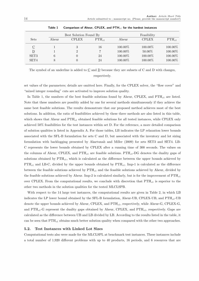
Table 1 Comparison of Aheur, CPLEX, and PTHs1 for the hardest instances

Best Solution Found By Feasibility

Sets Aheur CPLEX PTHs1 Aheur CPLEX PTHs1

C 1 3 16 100.00% 100.00% 100.00%

D 1 2 7 100.00% 50.00% 100.00%

SET3 6 0 24 100.00% 100.00% 100.00%

SET4 8 0 24 100.00% 100.00% 100.00%

The symbol of an underline is added to C and D because they are subsets of C and D with changes,

respectively.

set values of the parameters; details are omitted here. Finally, for the CPLEX solver, the “flow cover” and

“mixed integer rounding” cuts are activated to improve solution quality.

In Table 1, the numbers of the best feasible solutions found by Aheur, CPLEX, and PTHs1 are listed.

Note that these numbers are possibly added by one for several methods simultaneously if they achieve the

same best feasible solutions. The results demonstrate that our proposed method achieves most of the best

solutions. In addition, the ratio of feasibilities achieved by these three methods are also listed in this table,

which shows that Aheur and PTHs1 obtained feasible solutions for all tested instances, while CPLEX only

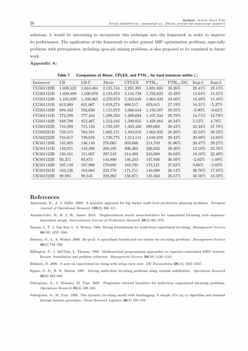
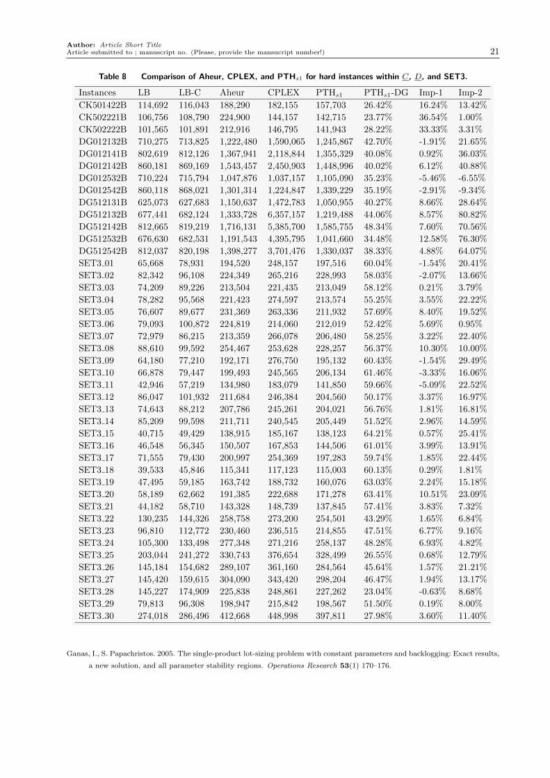
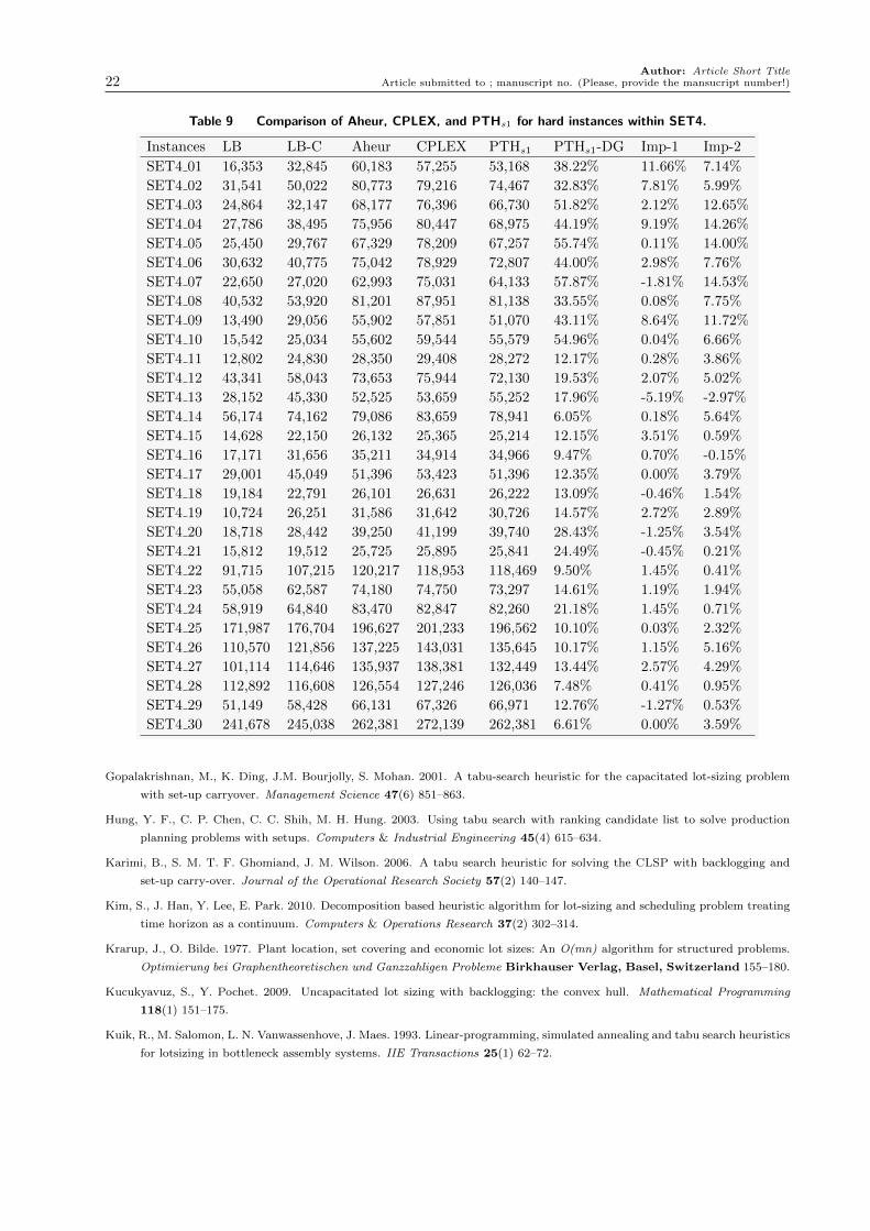
achieved 50% feasibilities for the test instances within set D. For the reference, a more detailed comparison

of solution qualities is listed in Appendix A. For those tables, LB indicates the LP relaxation lower bounds

associated with the SFL-B formulation for sets C and D, but associated with the inventory and lot sizing

formulation with backlogging presented by Akartunalı and Miller (2009) for sets SET3 and SET4. LB-

C represents the lower bounds obtained by CPLEX after a running time of 300 seconds. The values on

the columns of Aheur, CPLEX, and PTHs1 are feasible solutions. PTHs1-DG denotes the duality gaps of

solutions obtained by PTHs1, which is calculated as the difference between the upper bounds achieved by

PTHs1 and LB-C, divided by the upper bounds obtained by PTHs1. Imp-1 is calculated as the difference

between the feasible solutions achieved by PTHs1 and the feasible solutions achieved by Aheur, divided by

the feasible solutions achieved by Aheur. Imp-2 is calculated similarly, but is for the improvement of PTHs1

over CPLEX. From the computational results, we conclude with discretion that PTHs1 is superior to the

other two methods in the solution qualities for the tested MLCLSPB.

With respect to the 14 large test instances, the computational results are given in Table 2, in which LB

indicates the LP lower bound obtained by the SFL-B formulation, Aheur-UB, CPLEX-UB, and PTHs1-UB

denote the upper bounds achieved by Aheur, CPLEX, and PTHs1, respectively, while Aheur-G, CPLEX-G,

and PTHs1-G represent the duality gaps obtained by Aheur, CPLEX, and PTHs1, respectively. Gaps are

calculated as the difference between UB and LB divided by LB. According to the results listed in the table, it

can be seen that PTHs1 obtains much better solution quality when compared with the other two approaches.

5.2. Test Instances with Linked Lot Sizes

Computational tests also were made for the MLCLSPL at benchmark test instances. These instances include

a total number of 1,920 different problems with up to 40 products, 16 periods, and 6 resources that are


Table 2 Comparison of Aheur, CPLEX, and PTHs1 for large instances with 600 items, 90 machines, and 16

periods.

Instances LB Aheur-UB CPLEX-UB PTHs1-UB Aheur-G CPLEX-G PTHs1-G

EG501322 1007974.2 * 2165212.3 1234013.6 * 114.8% 22.4%

EG501332 611988.6 * 1110356.6 682980.9 * 81.4% 11.6%

EG501342 742285.9 1042958.0 1030618.1 818233.9 40.5% 38.8% 10.2%

EG501422 5692200.2 * 6916668.3 7064132.8 * 21.5% 24.1%

EG502322 1016122.5 * 2232185.7 1240374.8 * 119.7% 22.1%

EG502332 618685.4 * 1013634.6 681449.4 * 63.8% 10.1%

EG502422 10316942.9 * 11451008.4 10777368.2 * 11.0% 4.5%

EG502432 9848174.9 * 10332100.9 10072945.0 * 4.9% 2.3%

EG502442 9971797.3 * 10555222.5 10426393.6 * 5.9% 4.6%

EK501122 6229289.7 * 6383151.7 6369507.6 * 2.5% 2.3%

EK501322 140858.5 * 285081.1 171486.0 * 102.4% 21.7%

EK501332 85484.6 106953.1 139315.7 95071.5 25.1% 63.0% 11.2%

EK501342 96805.4 116890.6 145345.0 106748.4 20.7% 50.1% 10.3%

EK502332 84954.2 109279.6 127581.9 94295.6 28.6% 50.2% 11.0%

The symbol, *, represents that no solutions are found.

grouped into six classes with five factors, capacity, setup time, setup costs, demand variation, and bill-of-

materials structures. As the tests for larger size problems are more interesting, we choose test instances

in Classes 5 and 6 with setup costs that have a setting, 1, defined by Sahling et al. (2009), this is a total

number of 240 test instances. To show the efficiency of PTH, we made comparisons with the effective fix-

and-optimize (referred as FAO) method proposed by Tempelmeier and Buschkuhl (2009). The FAO method

was implemented in Delphi on a 2.13 GHz Intel Pentium Core2 machine, whereby the CPLEX 10.2 callable

library was used. To ensure a fair comparison, we directly used the same mixed integer model developed by

Sahling et al. (2009), and their best computational results, and implement PTHs1 in GAMS on a 1.7 GHz

PC. The computational time limit used by PTHs1 is set to 7.6 and 19.0 seconds for test instances in Classes

5 and 6, respectively, to match the average computational usage by the FAO method.

According to our computational tests, PTHs1 achieved better solution qualities compared with FAO. Out

of 120 instances we tested in Class 5, PHs1 achieved better solutions at 85 instances, tied solution qualities

at 25 instances, and obtained worse solution qualities at only 10 instances. Similarly, for the test instances in

Class 6, PHs1 achieved better solutions at 78 instances, tied solution qualities at 12 instances, and got worse

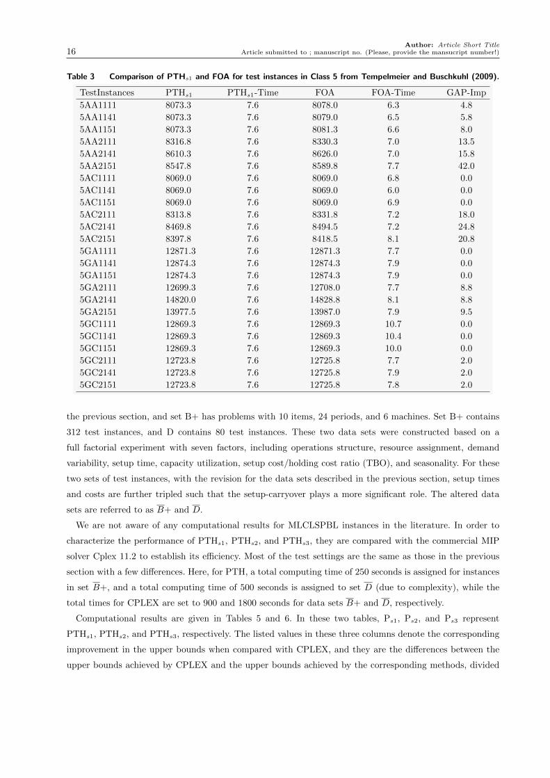
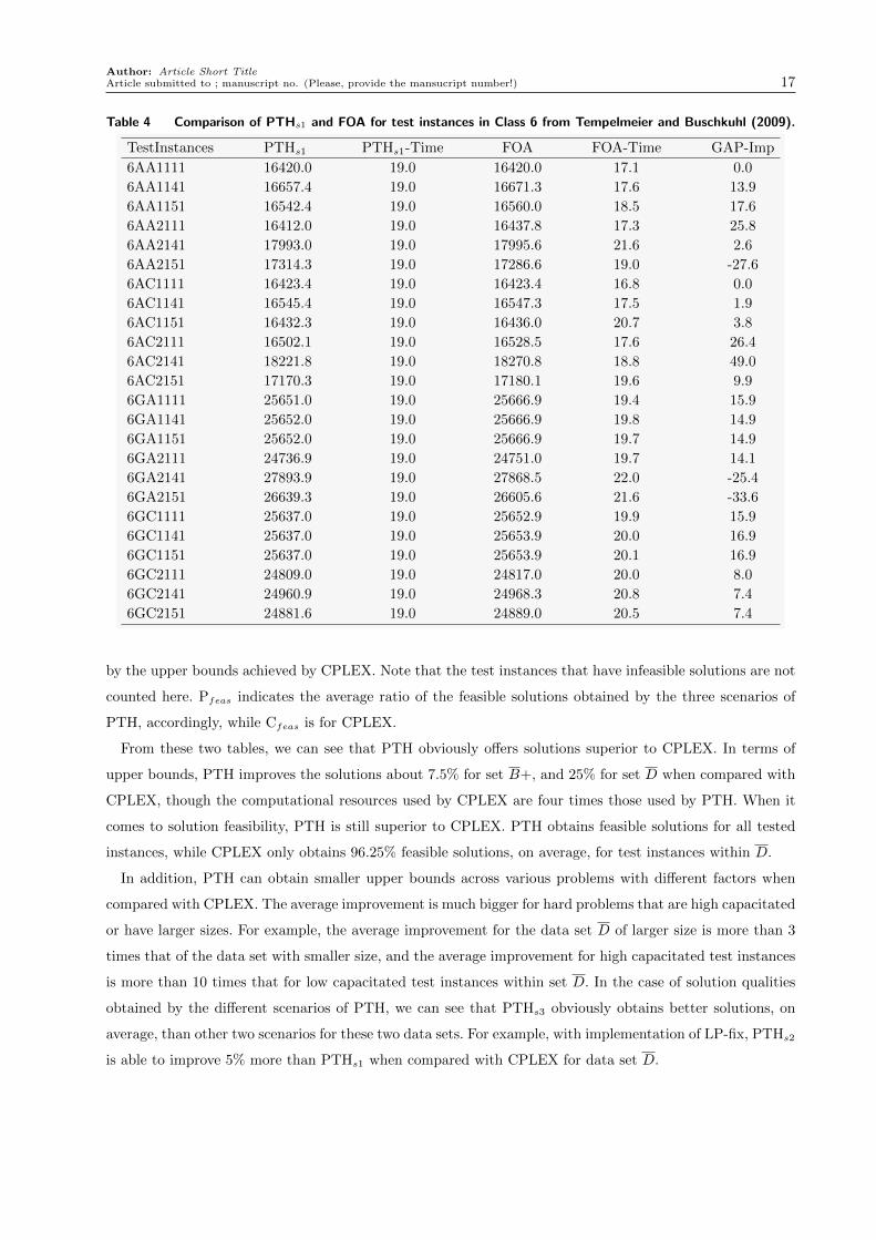
solution qualities at only 30 instances. For reference, we provide a partial set of solutions in Tables 3 and

4. In these two tables, the columns associated with PTHs1 and FOA provide objective solutions achieved

by these two methods, respectively, PTHs1-Time and FOA-Time indicate the computational time used by

these two methods, while GAP-Imp indicates the solution improved achieved by PTHs1 when compared with

FOA.

5.3. Test Instances with Backlogging and Linked Lot Sizes

In order to provide more computational insight, we selected all test instances within sets B+ and D with

setup times of Tempelmeier and Derstroff (1996) and Stadtler (2003). Set D has been briefly introduced in


Table 3 Comparison of PTHs1 and FOA for test instances in Class 5 from Tempelmeier and Buschkuhl (2009).

TestInstances PTHs1 PTHs1-Time FOA FOA-Time GAP-Imp

5AA1111 8073.3 7.6 8078.0 6.3 4.8

5AA1141 8073.3 7.6 8079.0 6.5 5.8

5AA1151 8073.3 7.6 8081.3 6.6 8.0

5AA2111 8316.8 7.6 8330.3 7.0 13.5

5AA2141 8610.3 7.6 8626.0 7.0 15.8

5AA2151 8547.8 7.6 8589.8 7.7 42.0

5AC1111 8069.0 7.6 8069.0 6.8 0.0

5AC1141 8069.0 7.6 8069.0 6.0 0.0

5AC1151 8069.0 7.6 8069.0 6.9 0.0

5AC2111 8313.8 7.6 8331.8 7.2 18.0

5AC2141 8469.8 7.6 8494.5 7.2 24.8

5AC2151 8397.8 7.6 8418.5 8.1 20.8

5GA1111 12871.3 7.6 12871.3 7.7 0.0

5GA1141 12874.3 7.6 12874.3 7.9 0.0

5GA1151 12874.3 7.6 12874.3 7.9 0.0

5GA2111 12699.3 7.6 12708.0 7.7 8.8

5GA2141 14820.0 7.6 14828.8 8.1 8.8

5GA2151 13977.5 7.6 13987.0 7.9 9.5

5GC1111 12869.3 7.6 12869.3 10.7 0.0

5GC1141 12869.3 7.6 12869.3 10.4 0.0

5GC1151 12869.3 7.6 12869.3 10.0 0.0

5GC2111 12723.8 7.6 12725.8 7.7 2.0

5GC2141 12723.8 7.6 12725.8 7.9 2.0

5GC2151 12723.8 7.6 12725.8 7.8 2.0

the previous section, and set B+ has problems with 10 items, 24 periods, and 6 machines. Set B+ contains

312 test instances, and D contains 80 test instances. These two data sets were constructed based on a

full factorial experiment with seven factors, including operations structure, resource assignment, demand

variability, setup time, capacity utilization, setup cost/holding cost ratio (TBO), and seasonality. For these

two sets of test instances, with the revision for the data sets described in the previous section, setup times

and costs are further tripled such that the setup-carryover plays a more significant role. The altered data

sets are referred to as B+ and D.

We are not aware of any computational results for MLCLSPBL instances in the literature. In order to

characterize the performance of PTHs1, PTHs2, and PTHs3, they are compared with the commercial MIP

solver Cplex 11.2 to establish its efficiency. Most of the test settings are the same as those in the previous

section with a few differences. Here, for PTH, a total computing time of 250 seconds is assigned for instances

in set B+, and a total computing time of 500 seconds is assigned to set D (due to complexity), while the

total times for CPLEX are set to 900 and 1800 seconds for data sets B+ and D, respectively.

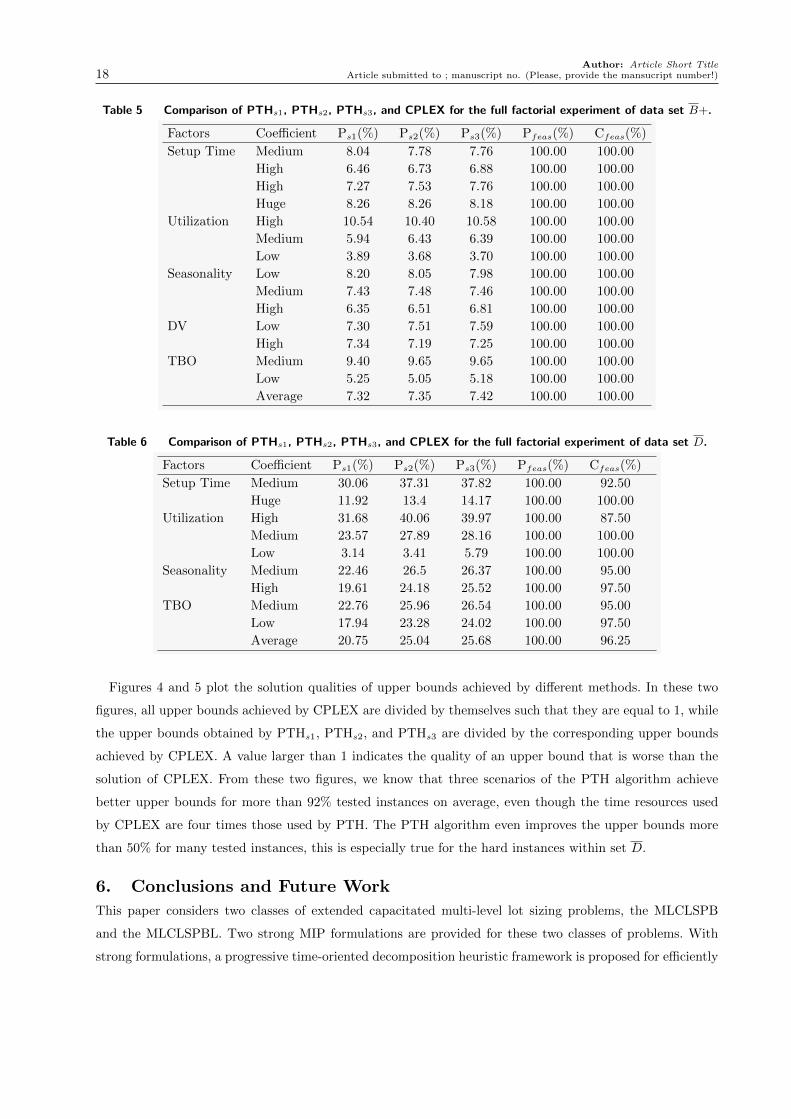
Computational results are given in Tables 5 and 6. In these two tables, Ps1, Ps2, and Ps3 represent

PTHs1, PTHs2, and PTHs3, respectively. The listed values in these three columns denote the corresponding

improvement in the upper bounds when compared with CPLEX, and they are the differences between the

upper bounds achieved by CPLEX and the upper bounds achieved by the corresponding methods, divided


Table 4 Comparison of PTHs1 and FOA for test instances in Class 6 from Tempelmeier and Buschkuhl (2009).

TestInstances PTHs1 PTHs1-Time FOA FOA-Time GAP-Imp

6AA1111 16420.0 19.0 16420.0 17.1 0.0

6AA1141 16657.4 19.0 16671.3 17.6 13.9

6AA1151 16542.4 19.0 16560.0 18.5 17.6

6AA2111 16412.0 19.0 16437.8 17.3 25.8

6AA2141 17993.0 19.0 17995.6 21.6 2.6

6AA2151 17314.3 19.0 17286.6 19.0 -27.6

6AC1111 16423.4 19.0 16423.4 16.8 0.0

6AC1141 16545.4 19.0 16547.3 17.5 1.9

6AC1151 16432.3 19.0 16436.0 20.7 3.8

6AC2111 16502.1 19.0 16528.5 17.6 26.4

6AC2141 18221.8 19.0 18270.8 18.8 49.0

6AC2151 17170.3 19.0 17180.1 19.6 9.9

6GA1111 25651.0 19.0 25666.9 19.4 15.9

6GA1141 25652.0 19.0 25666.9 19.8 14.9

6GA1151 25652.0 19.0 25666.9 19.7 14.9

6GA2111 24736.9 19.0 24751.0 19.7 14.1

6GA2141 27893.9 19.0 27868.5 22.0 -25.4

6GA2151 26639.3 19.0 26605.6 21.6 -33.6

6GC1111 25637.0 19.0 25652.9 19.9 15.9

6GC1141 25637.0 19.0 25653.9 20.0 16.9

6GC1151 25637.0 19.0 25653.9 20.1 16.9

6GC2111 24809.0 19.0 24817.0 20.0 8.0

6GC2141 24960.9 19.0 24968.3 20.8 7.4

6GC2151 24881.6 19.0 24889.0 20.5 7.4

by the upper bounds achieved by CPLEX. Note that the test instances that have infeasible solutions are not

counted here. Pfeas indicates the average ratio of the feasible solutions obtained by the three scenarios of

PTH, accordingly, while Cfeas is for CPLEX.

From these two tables, we can see that PTH obviously offers solutions superior to CPLEX. In terms of

upper bounds, PTH improves the solutions about 7.5% for set B+, and 25% for set D when compared with

CPLEX, though the computational resources used by CPLEX are four times those used by PTH. When it

comes to solution feasibility, PTH is still superior to CPLEX. PTH obtains feasible solutions for all tested

instances, while CPLEX only obtains 96.25% feasible solutions, on average, for test instances within D.

In addition, PTH can obtain smaller upper bounds across various problems with different factors when

compared with CPLEX. The average improvement is much bigger for hard problems that are high capacitated

or have larger sizes. For example, the average improvement for the data set D of larger size is more than 3

times that of the data set with smaller size, and the average improvement for high capacitated test instances

is more than 10 times that for low capacitated test instances within set D. In the case of solution qualities

obtained by the different scenarios of PTH, we can see that PTHs3 obviously obtains better solutions, on

average, than other two scenarios for these two data sets. For example, with implementation of LP-fix, PTHs2

is able to improve 5% more than PTHs1 when compared with CPLEX for data set D.


Table 5 Comparison of PTHs1, PTHs2, PTHs3, and CPLEX for the full factorial experiment of data set B+.

Factors Coefficient Ps1(%) Ps2(%) Ps3(%) Pfeas(%) Cfeas(%)

Setup Time Medium 8.04 7.78 7.76 100.00 100.00

High 6.46 6.73 6.88 100.00 100.00

High 7.27 7.53 7.76 100.00 100.00

Huge 8.26 8.26 8.18 100.00 100.00

Utilization High 10.54 10.40 10.58 100.00 100.00

Medium 5.94 6.43 6.39 100.00 100.00

Low 3.89 3.68 3.70 100.00 100.00

Seasonality Low 8.20 8.05 7.98 100.00 100.00

Medium 7.43 7.48 7.46 100.00 100.00

High 6.35 6.51 6.81 100.00 100.00

DV Low 7.30 7.51 7.59 100.00 100.00

High 7.34 7.19 7.25 100.00 100.00

TBO Medium 9.40 9.65 9.65 100.00 100.00

Low 5.25 5.05 5.18 100.00 100.00

Average 7.32 7.35 7.42 100.00 100.00

Table 6 Comparison of PTHs1, PTHs2, PTHs3, and CPLEX for the full factorial experiment of data set D.

Factors Coefficient Ps1(%) Ps2(%) Ps3(%) Pfeas(%) Cfeas(%)

Setup Time Medium 30.06 37.31 37.82 100.00 92.50

Huge 11.92 13.4 14.17 100.00 100.00

Utilization High 31.68 40.06 39.97 100.00 87.50

Medium 23.57 27.89 28.16 100.00 100.00

Low 3.14 3.41 5.79 100.00 100.00

Seasonality Medium 22.46 26.5 26.37 100.00 95.00

High 19.61 24.18 25.52 100.00 97.50

TBO Medium 22.76 25.96 26.54 100.00 95.00

Low 17.94 23.28 24.02 100.00 97.50

Average 20.75 25.04 25.68 100.00 96.25

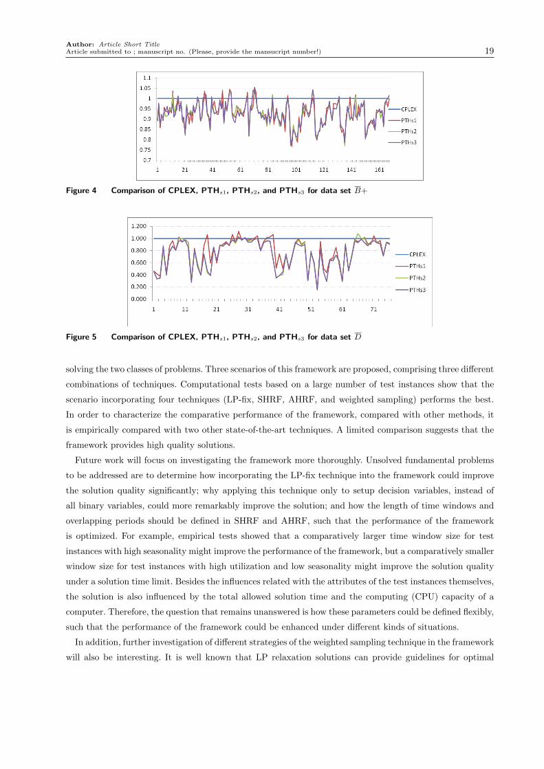
Figures 4 and 5 plot the solution qualities of upper bounds achieved by different methods. In these two

figures, all upper bounds achieved by CPLEX are divided by themselves such that they are equal to 1, while

the upper bounds obtained by PTHs1, PTHs2, and PTHs3 are divided by the corresponding upper bounds

achieved by CPLEX. A value larger than 1 indicates the quality of an upper bound that is worse than the

solution of CPLEX. From these two figures, we know that three scenarios of the PTH algorithm achieve

better upper bounds for more than 92% tested instances on average, even though the time resources used

by CPLEX are four times those used by PTH. The PTH algorithm even improves the upper bounds more

than 50% for many tested instances, this is especially true for the hard instances within set D.

6. Conclusions and Future Work

This paper considers two classes of extended capacitated multi-level lot sizing problems, the MLCLSPB

and the MLCLSPBL. Two strong MIP formulations are provided for these two classes of problems. With

strong formulations, a progressive time-oriented decomposition heuristic framework is proposed for efficiently


Figure 4 Comparison of CPLEX, PTHs1, PTHs2, and PTHs3 for data set B+

Figure 5 Comparison of CPLEX, PTHs1, PTHs2, and PTHs3 for data set D

solving the two classes of problems. Three scenarios of this framework are proposed, comprising three different

combinations of techniques. Computational tests based on a large number of test instances show that the

scenario incorporating four techniques (LP-fix, SHRF, AHRF, and weighted sampling) performs the best.

In order to characterize the comparative performance of the framework, compared with other methods, it

is empirically compared with two other state-of-the-art techniques. A limited comparison suggests that the

framework provides high quality solutions.

Future work will focus on investigating the framework more thoroughly. Unsolved fundamental problems

to be addressed are to determine how incorporating the LP-fix technique into the framework could improve

the solution quality significantly; why applying this technique only to setup decision variables, instead of

all binary variables, could more remarkably improve the solution; and how the length of time windows and

overlapping periods should be defined in SHRF and AHRF, such that the performance of the framework

is optimized. For example, empirical tests showed that a comparatively larger time window size for test

instances with high seasonality might improve the performance of the framework, but a comparatively smaller

window size for test instances with high utilization and low seasonality might improve the solution quality

under a solution time limit. Besides the influences related with the attributes of the test instances themselves,

the solution is also influenced by the total allowed solution time and the computing (CPU) capacity of a

computer. Therefore, the question that remains unanswered is how these parameters could be defined flexibly,

such that the performance of the framework could be enhanced under different kinds of situations.

In addition, further investigation of different strategies of the weighted sampling technique in the framework

will also be interesting. It is well known that LP relaxation solutions can provide guidelines for optimal


solutions; it would be interesting to incorporate this technique into the framework in order to improve

its performance. The application of the framework to other general MIP optimization problems, especially

problems with prerequisites, including open-pit mining problems, is also proposed to be examined in future

work.

Appendix A:

Table 7 Comparison of Aheur, CPLEX, and PTHs1 for hard instances within C.

Instances LB LB-C Aheur CPLEX PTHs1 PTHs1-DG Imp-1 Imp-2

CG501120B 1,039,522 1,044,484 2,125,744 2,201,391 1,691,803 38.26% 20.41% 23.15%

CG501121B 1,028,889 1,030,976 2,125,073 2,116,728 1,792,622 42.49% 15.64% 15.31%

CG501122B 1,105,629 1,108,865 2,270,973 2,323,648 1,964,833 43.56% 13.48% 15.44%

CG501131B 613,969 621,067 1,019,274 809,517 853,015 27.19% 16.31% -5.37%

CG501132B 694,442 702,630 1,115,072 1,066,644 1,158,587 39.35% -3.90% -8.62%

CG501141B 773,599 777,444 1,298,350 1,269,694 1,107,344 29.79% 14.71% 12.79%

CG501142B 848,798 852,467 1,512,416 1,500,655 1,428,884 40.34% 5.52% 4.78%

CG501222B 710,289 715,123 1,729,587 1,383,430 999,069 28.42% 42.24% 27.78%

CG502221B 759,515 764,581 1,602,151 1,483,852 1,064,932 28.20% 33.53% 28.23%

CG502222B 734,617 739,676 1,720,775 1,214,141 1,048,070 29.42% 39.09% 13.68%

CK501120B 145,805 146,140 270,065 303,666 214,783 31.96% 20.47% 29.27%

CK501121B 143,071 143,398 269,195 306,362 236,632 39.40% 12.10% 22.76%

CK501122B 150,161 151,007 297,545 314,389 243,688 38.03% 18.10% 22.49%

CK501132B 93,371 93,875 144,896 146,243 147,826 36.50% -2.02% -1.08%

CK501142B 107,149 107,996 179,695 163,795 173,121 37.62% 3.66% -5.69%

CK501221B 103,136 104,064 222,778 171,711 140,890 26.14% 36.76% 17.95%

CK501222B 98,985 99,545 228,062 156,871 135,563 26.57% 40.56% 13.58%

ReferencesAkartunalı, K., A. J. Miller. 2009. A heuristic approach for big bucket multi-level production planning problems. European

Journal of Operational Research 193(2) 396–411.

Almada-Lobo, B., R. J. W. James. 2010. Neighbourhood search meta-heuristics for capacitated lot-sizing with sequence-

dependent setups. International Journal of Production Research 48(3) 861–878.

Barany, I., T. J. Van Roy, L. A. Wolsey. 1984. Strong formulations for multi-item capacitated lot-sizing. Management Science

30(10) 1255–1261.

Belvaux, G., L. A. Wolsey. 2000. Bc-prod: A specialized branch-and-cut system for lot-sizing problems. Management Science

46(5) 724–738.

Billington, P., J. McClain, L. Thomas. 1983. Mathematical programming approaches to capacity-constrained MRP systems:

Review, formulation and problem reduction. Management Science 29(10) 1126–1141.

Briskorn, D. 2006. A note on capacitated lot sizing with setup carry over. IIE Transactions 38(11) 1045–1047.

Eppen, G. D., R. K. Martin. 1987. Solving multi-item lot-sizing problems using variable redefinition. Operations Research

35(6) 832–848.

Federgruen, A., J. Meissner, M. Tzur. 2007. Progressive interval heuristics for multi-item capacitated lot-sizing problems.

Operations Research 55(3) 490–502.

Federgruen, A., M. Tzur. 1993. The dynamic lot-sizing model with backlogging: A simple O(n log n) algorithm and minimal

forecast horizon procedure. Naval Research Logistics 40(4) 459–478.


Table 8 Comparison of Aheur, CPLEX, and PTHs1 for hard instances within C, D, and SET3.


CK501422B 114,692 116,043 188,290 182,155 157,703 26.42% 16.24% 13.42%

CK502221B 106,756 108,790 224,900 144,157 142,715 23.77% 36.54% 1.00%

CK502222B 101,565 101,891 212,916 146,795 141,943 28.22% 33.33% 3.31%

DG012132B 710,275 713,825 1,222,480 1,590,065 1,245,867 42.70% -1.91% 21.65%

DG012141B 802,619 812,126 1,367,941 2,118,844 1,355,329 40.08% 0.92% 36.03%

DG012142B 860,181 869,169 1,543,457 2,450,903 1,448,996 40.02% 6.12% 40.88%

DG012532B 710,224 715,794 1,047,876 1,037,157 1,105,090 35.23% -5.46% -6.55%

DG012542B 860,118 868,021 1,301,314 1,224,847 1,339,229 35.19% -2.91% -9.34%

DG512131B 625,073 627,683 1,150,637 1,472,783 1,050,955 40.27% 8.66% 28.64%

DG512132B 677,441 682,124 1,333,728 6,357,157 1,219,488 44.06% 8.57% 80.82%

DG512142B 812,665 819,219 1,716,131 5,385,700 1,585,755 48.34% 7.60% 70.56%

DG512532B 676,630 682,531 1,191,543 4,395,795 1,041,660 34.48% 12.58% 76.30%

DG512542B 812,037 820,198 1,398,277 3,701,476 1,330,037 38.33% 4.88% 64.07%

SET3 01 65,668 78,931 194,520 248,157 197,516 60.04% -1.54% 20.41%

SET3 02 82,342 96,108 224,349 265,216 228,993 58.03% -2.07% 13.66%

SET3 03 74,209 89,226 213,504 221,435 213,049 58.12% 0.21% 3.79%

SET3 04 78,282 95,568 221,423 274,597 213,574 55.25% 3.55% 22.22%

SET3 05 76,607 89,677 231,369 263,336 211,932 57.69% 8.40% 19.52%

SET3 06 79,093 100,872 224,819 214,060 212,019 52.42% 5.69% 0.95%

SET3 07 72,979 86,215 213,359 266,078 206,480 58.25% 3.22% 22.40%

SET3 08 88,610 99,592 254,467 253,628 228,257 56.37% 10.30% 10.00%

SET3 09 64,180 77,210 192,171 276,750 195,132 60.43% -1.54% 29.49%

SET3 10 66,878 79,447 199,493 245,565 206,134 61.46% -3.33% 16.06%

SET3 11 42,946 57,219 134,980 183,079 141,850 59.66% -5.09% 22.52%

SET3 12 86,047 101,932 211,684 246,384 204,560 50.17% 3.37% 16.97%

SET3 13 74,643 88,212 207,786 245,261 204,021 56.76% 1.81% 16.81%

SET3 14 85,209 99,598 211,711 240,545 205,449 51.52% 2.96% 14.59%

SET3 15 40,715 49,429 138,915 185,167 138,123 64.21% 0.57% 25.41%

SET3 16 46,548 56,345 150,507 167,853 144,506 61.01% 3.99% 13.91%

SET3 17 71,555 79,430 200,997 254,369 197,283 59.74% 1.85% 22.44%

SET3 18 39,533 45,846 115,341 117,123 115,003 60.13% 0.29% 1.81%

SET3 19 47,495 59,185 163,742 188,732 160,076 63.03% 2.24% 15.18%

SET3 20 58,189 62,662 191,385 222,688 171,278 63.41% 10.51% 23.09%

SET3 21 44,182 58,710 143,328 148,739 137,845 57.41% 3.83% 7.32%

SET3 22 130,235 144,326 258,758 273,200 254,501 43.29% 1.65% 6.84%

SET3 23 96,810 112,772 230,460 236,515 214,855 47.51% 6.77% 9.16%

SET3 24 105,300 133,498 277,348 271,216 258,137 48.28% 6.93% 4.82%

SET3 25 203,044 241,272 330,743 376,654 328,499 26.55% 0.68% 12.79%

SET3 26 145,184 154,682 289,107 361,160 284,564 45.64% 1.57% 21.21%

SET3 27 145,420 159,615 304,090 343,420 298,204 46.47% 1.94% 13.17%

SET3 28 145,227 174,909 225,838 248,861 227,262 23.04% -0.63% 8.68%

SET3 29 79,813 96,308 198,947 215,842 198,567 51.50% 0.19% 8.00%

SET3 30 274,018 286,496 412,668 448,998 397,811 27.98% 3.60% 11.40%

Ganas, I., S. Papachristos. 2005. The single-product lot-sizing problem with constant parameters and backlogging: Exact results,

a new solution, and all parameter stability regions. Operations Research 53(1) 170–176.


Table 9 Comparison of Aheur, CPLEX, and PTHs1 for hard instances within SET4.


SET4 01 16,353 32,845 60,183 57,255 53,168 38.22% 11.66% 7.14%

SET4 02 31,541 50,022 80,773 79,216 74,467 32.83% 7.81% 5.99%

SET4 03 24,864 32,147 68,177 76,396 66,730 51.82% 2.12% 12.65%

SET4 04 27,786 38,495 75,956 80,447 68,975 44.19% 9.19% 14.26%

SET4 05 25,450 29,767 67,329 78,209 67,257 55.74% 0.11% 14.00%

SET4 06 30,632 40,775 75,042 78,929 72,807 44.00% 2.98% 7.76%

SET4 07 22,650 27,020 62,993 75,031 64,133 57.87% -1.81% 14.53%

SET4 08 40,532 53,920 81,201 87,951 81,138 33.55% 0.08% 7.75%

SET4 09 13,490 29,056 55,902 57,851 51,070 43.11% 8.64% 11.72%

SET4 10 15,542 25,034 55,602 59,544 55,579 54.96% 0.04% 6.66%

SET4 11 12,802 24,830 28,350 29,408 28,272 12.17% 0.28% 3.86%

SET4 12 43,341 58,043 73,653 75,944 72,130 19.53% 2.07% 5.02%

SET4 13 28,152 45,330 52,525 53,659 55,252 17.96% -5.19% -2.97%

SET4 14 56,174 74,162 79,086 83,659 78,941 6.05% 0.18% 5.64%

SET4 15 14,628 22,150 26,132 25,365 25,214 12.15% 3.51% 0.59%

SET4 16 17,171 31,656 35,211 34,914 34,966 9.47% 0.70% -0.15%

SET4 17 29,001 45,049 51,396 53,423 51,396 12.35% 0.00% 3.79%

SET4 18 19,184 22,791 26,101 26,631 26,222 13.09% -0.46% 1.54%

SET4 19 10,724 26,251 31,586 31,642 30,726 14.57% 2.72% 2.89%

SET4 20 18,718 28,442 39,250 41,199 39,740 28.43% -1.25% 3.54%

SET4 21 15,812 19,512 25,725 25,895 25,841 24.49% -0.45% 0.21%

SET4 22 91,715 107,215 120,217 118,953 118,469 9.50% 1.45% 0.41%

SET4 23 55,058 62,587 74,180 74,750 73,297 14.61% 1.19% 1.94%

SET4 24 58,919 64,840 83,470 82,847 82,260 21.18% 1.45% 0.71%

SET4 25 171,987 176,704 196,627 201,233 196,562 10.10% 0.03% 2.32%

SET4 26 110,570 121,856 137,225 143,031 135,645 10.17% 1.15% 5.16%

SET4 27 101,114 114,646 135,937 138,381 132,449 13.44% 2.57% 4.29%

SET4 28 112,892 116,608 126,554 127,246 126,036 7.48% 0.41% 0.95%

SET4 29 51,149 58,428 66,131 67,326 66,971 12.76% -1.27% 0.53%

SET4 30 241,678 245,038 262,381 272,139 262,381 6.61% 0.00% 3.59%

Gopalakrishnan, M., K. Ding, J.M. Bourjolly, S. Mohan. 2001. A tabu-search heuristic for the capacitated lot-sizing problem

with set-up carryover. Management Science 47(6) 851–863.

Hung, Y. F., C. P. Chen, C. C. Shih, M. H. Hung. 2003. Using tabu search with ranking candidate list to solve production

planning problems with setups. Computers & Industrial Engineering 45(4) 615–634.

Karimi, B., S. M. T. F. Ghomiand, J. M. Wilson. 2006. A tabu search heuristic for solving the CLSP with backlogging and

set-up carry-over. Journal of the Operational Research Society 57(2) 140–147.

Kim, S., J. Han, Y. Lee, E. Park. 2010. Decomposition based heuristic algorithm for lot-sizing and scheduling problem treating

time horizon as a continuum. Computers & Operations Research 37(2) 302–314.

Krarup, J., O. Bilde. 1977. Plant location, set covering and economic lot sizes: An O(mn) algorithm for structured problems.

Optimierung bei Graphentheoretischen und Ganzzahligen Probleme Birkhauser Verlag, Basel, Switzerland 155–180.

Kucukyavuz, S., Y. Pochet. 2009. Uncapacitated lot sizing with backlogging: the convex hull. Mathematical Programming

118(1) 151–175.

Kuik, R., M. Salomon, L. N. Vanwassenhove, J. Maes. 1993. Linear-programming, simulated annealing and tabu search heuristics

for lotsizing in bottleneck assembly systems. IIE Transactions 25(1) 62–72.


Mathieu, V. V. 2006. Linear-programming extended formulations for the single-item lot-sizing problem with backlogging and

constant capacity. Mathematical Programming 108(1) 53–77.

Millar, H. H., M. Z. Yang. 1994. Lagrangian heuristics for the capacitated multiitem lot-sizing problem with backordering.

International Journal of Production Economics 34(1) 1–15.

Miller, A. J., L. A. Wolsey. 2003. Tight MIP formulations for multi-item discrete lot-sizing problems. Operations Research

51(4) 557–565.

Pochet, Y., L. A. Wolsey. 1988. Lot-size models with backlogging: Strong reformulations and cutting planes. Mathematical

Programming 40(3) 317–335.

Pochet, Y., L. A. Wolsey. 1991. Solving multi-item lot-sizing problems using strong cutting planes. Management Science 37(1)

53–67.

Sahling, F., L. Buschkuhl, H. Tempelmeier, S. Helber. 2009. Solving a multi-level capacitated lot sizing problem with multi-

period setup carry-over via a fix-and-optimize heuristic. Computers & Operations Research 36(9) 2546–2553.

Simpson, N.C., S.S. Erenguc. 2005. Modeling multiple stage manufacturing systems with generalized costs and capacity issues.

Naval Research Logistics 52(6) 560570.

Song, Y.Y., G.H. Chan. 2005. Single item lot-sizing problems with backlogging on a single machine at a finite production rate.

European Journal of Operational Research 161(1) 191–202.

Sox, C.R., Y.B. Gao. 1999. The capacitated lot sizing problem with setup carry-over. IIE Transactions 31(2) 173–181.

Stadtler, H. 2003. Multilevel lot sizing with setup times and multiple constrained resources: Internally rolling schedules with

lot-sizing windows. Operations Research 51(3) 487–502.

Suerie, C., H. Stadtler. 2003. The capacitated lot-sizing with linked lot sizes. Management Science 49(8) 1039–1054.

Tempelmeier, H., L. Buschkuhl. 2009. A heuristic for the dynamic multi-level capacitated lotsizing problem with linked lotsizes

for general product structures. OR Spectrum 31(2) 385–404.

Tempelmeier, H., M. Derstroff. 1996. A lagrangian-based heuristic for dynamic multilevel multiitem constrained lotsizing with

setup times. Management Science 42(5) 738–757.

mixed integer programming in production planning with bill...

Documents