Analysis of Bounds for a Capacitated Single-item

Lot-sizing Problem

Jill R. Hardin ?†

George L. Nemhauser ??

Martin W. P. Savelsbergh ??

? Department of Statistical Sciences and Operations ResearchVirginia Commonwealth University

1001 West Main StreetP.O. Box 843083

Richmond, VA 23284-3083jrhardin@vcu.edu

?? School of Industrial and Systems EngineeringGeorgia Institute of Technology

765 Ferst Drive, NWAtlanta, GA 30332-0205

{george.nemhauser,martin.savelsbergh}@isye.gatech.edu

Abstract

Lot-sizing problems are cornerstone optimization problems for production planningwith time varying demand. We analyze the quality of bounds, both lower and upper,provided by a range of fast algorithms. Special attention is given to LP-based roundingalgorithms.

1 Introduction

Lot-sizing problems have attracted attention for decades because they form the cornerstoneoptimization problems for production planning with time varying demand (the economicorder quantity model being the cornerstone optimization problem for production planningwith stationary demand). One of the chief difficulties in solving lot-sizing problems arisesfrom capacity restrictions in each time period. In fact, the problem is polynomially solvablewhen capacities are absent [19], as well as when production capacities are identical in eachperiod of the planning horizon [5]. When capacities are allowed to vary over the planninghorizon, however, the problem is NP-hard.

Lot-sizing problems are well studied. A good exact approach for the single-item lot-sizing problem with general capacities comes from Chen & Lee [3], who provide a dynamic

†Corresponding author

1

program to solve it. Polyhedral results for these problems are especially plentiful. Notableresults are found in, among others, [9], [12], and [13] (see [10] for a more comprehensivereview). The abundance of polyhedral results has resulted in more effective integer pro-gramming based solution approaches, but many instances still require prohibitive amountsof computation time. Van Hoesel & Wagelmans [17] approach the problem differently andpresent a fully polynomial approximation scheme for single-item capacitated lot-sizing,with the time required to find a solution depending on the desired nearness of the valueof the resulting solution to the optimal value. Unfortunately, the practical value of thisapproach is limited as the computational requirements are high even for moderate approx-imation factors.

Therefore, we focus our efforts on developing quick procedures that provide qualitybounds (both lower and upper) for lot-sizing problems. We pared the problem down toits simplest form by assuming the absence of unit production and holding costs. The onlyfactors then influencing solution feasibility and quality are the setup costs and productioncapacities. By doing so, we hope to gain better understanding of the interaction betweensetup costs and capacities and how they influence the quality of bounding and solutiontechniques. This variant of the lot-sizing problem is polynomially solvable when the in-stance data satisfy certain conditions. For instance, when capacities are nonincreasing andsetup costs are nondecreasing over time, then the problem can be easily solved. However,when capacities and setup costs are allowed to vary arbitrarily the problem is NP-hard(see [2] for a more thorough discussion of complexity results for capacitated lot-sizing).

Another motivation for studying approximation algorithms for lot-sizing problems isthe recent success of LP-based approximation algorithms for a variety of discrete opti-mization problems [18], in particular scheduling problems ([1, 6, 7, 14, 15], to name afew). Given the serial component common to both scheduling and lot-sizing problems, itis natural to investigate the potential of LP-based techniques for lot-sizing problems.

We begin, in Section 2, by formally defining the problem we consider, by identifyingassumptions we make throughout the paper, and by presenting the integer programmingformulation on which our studies are based. Then, in Section 3, we examine a specialcase of the problem, providing a polynomial-time algorithm to solve it. Subsequently, inSection 4, we return to the general case and study various lower bounds. We start bypresenting an algorithm to solve the LP relaxation in quadratic time. Next, we analyzethe strength of the LP relaxation, of a ratio-based lower bound inspired by our algorithmto solve the LP relaxation, and of a constant capacity relaxation. Following the studyof lower bounds, we introduce, in Section 5, several upper bounds based on LP roundingand one upper bound inspired by our algorithm to solve the LP relaxation, offering aworst-case analysis of each.

The performance guarantees derived are data dependent. The typical guarantee is thatthe relative deviation from the optimal value is not larger than the maximum capacity.Even though such guarantees may be weak, they are shown to be tight. Therefore, it

2

appears unlikely that the success of LP-based approximations algorithms can easily bereplicated in the context of lot-sizing problems.

2 Problem Description (LSZIP)

For each period t in the discrete planning horizon {1, . . . , T}, we are given demand dt,production capacity Ct, and cost ft which is incurred if any positive level of productiontakes place in period t. The objective, then, is to schedule production that respects allcapacities and satisfies all demands, where production in period t may be used to satisfydemand in any of periods {t, . . . , T}. We denote this problem LSZIP. Let dst = ds+· · ·+dt

for 1 ≤ s ≤ t ≤ T , and

yt ={

1 if production takes place in period t0 otherwise.

Our studies are based on the following integer programming formulation for LSZIP:

minT∑

t=1

ftyt (1)

t∑i=1

Ciyi ≥ d1t t ∈ {1, . . . , T} (2)

yt ∈ {0, 1} t ∈ {1, . . . , T}. (3)

Note that since production and inventory costs are zero, we may assume that production inany period takes place at capacity or not at all. Constraints (2) ensure that, in any periodt, enough production has been scheduled to meet demand up to that point. Constraints(3) ensure that we pay the entire setup cost if any positive level of production is scheduledin a given period.

We assume integral data throughout. We define Cmax = max{Ct : t ∈ {1, . . . , T}},fmax = max{ft : t ∈ {1, . . . , T}}, and fmin = min{ft : t ∈ {1, . . . , T}}. Furthermore, werefer to the formulation (1)–(3) as IPLS , and we assume

• Ct ≤ dtT . Since production can only be used to satisfy demand in present and futureperiods, we will never need to produce more than dtT in period t.

• dT > 0. If dT = 0, then production in period T cannot satisfy any demand, thus wemay solve the problem limited to time horizon {1, . . . , T − 1}.

• ft > 0. Since we are minimizing total cost, if ft ≤ 0, we can fix yt = 1.

3

We let yIP and zIP denote, respectively, an optimal solution to IPLS and its objectivevalue. For convenience, we will often say that a set S ⊆ {1, . . . , T} is a solution to IPLS .By this, we mean that the solution given by yt = 1 ⇔ t ∈ S is a solution to IPLS . Also,when discussing a solution y of IPLS , we say that period t is open if yt = 1, and closed ifyt = 0.

When considering upper bounding methods, it is useful to analyze the quality of thesolutions they provide. Suppose we wish to solve an NP-hard minimization problemconsisting of instances in I. For each instance I ∈ I, let z(I) denote the objective valueof an optimal solution. Furthermore, let A be an algorithm that operates on instances inI, and let A(I) be the objective value resulting from the application of A to I. Let ρ ≥ 1and assume z(I) > 0.

Definition 1. A is a ρ-approximation algorithm for I if for each I ∈ I, A(I) ≤ ρz(I). Ais also said to have approximation factor ρ.

Note that the approximation factor ρ is defined by comparison with z(I), the optimalvalue for instance I. Direct comparison with z(I), however, is impractical, since if weknow z(I) there is no need to approximate it. In light of this observation, the validity ofρ is established in practice via comparison with a lower bound for z(I). Let L(I) be sucha lower bound. Then

A(I) ≤ ρL(I) =⇒ A(I) ≤ ρz(I).

Definition 2. The approximation factor ρ is said to be tight if for any ε > 0, there existsan I ∈ I such that A(I) ≥ ρz(I)− ε.

Proving that ρ is tight for A reveals that, if any improvement is to be made to ρ, thealgorithm, and not its analysis, must be refined. In order to establish that ρ is tight, wemust construct tight examples.

Definition 3. A sequence I(n) ⊆ I is said to be a sequence of tight examples if

limn→∞

ρz(I(n))−A(I(n)) = 0.

In the definitions above, it has been assumed that the approximation factor ρ is aconstant that is independent of the instance data. In our analysis, we derive approximationfactors that do depend on the instance data, typically on Cmax. Making statements aboutthe tightness of an approximation factor Cmax is more difficult, because Cmax can takeon many values depending on the instance data. In such situations, the following types ofresults are of interest. First, it may be possible to show that there exist values of Cmax

for which there exist instances for which the approximation factor Cmax is tight. Second,it may be possible to show that the ratio A(I)/z(I) grows with Cmax. Finally, it may bepossible to show that for every integer k > 1 and every ε > 0, there exist instances withCmax = k, and A(I) ≥ kz(I)− ε.

4

3 A Polynomially Solvable Case

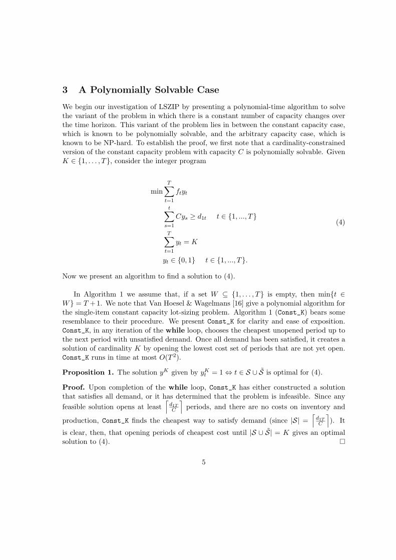
We begin our investigation of LSZIP by presenting a polynomial-time algorithm to solvethe variant of the problem in which there is a constant number of capacity changes overthe time horizon. This variant of the problem lies in between the constant capacity case,which is known to be polynomially solvable, and the arbitrary capacity case, which isknown to be NP-hard. To establish the proof, we first note that a cardinality-constrainedversion of the constant capacity problem with capacity C is polynomially solvable. GivenK ∈ {1, . . . , T}, consider the integer program

minT∑

t=1

ftyt

t∑s=1

Cys ≥ d1t t ∈ {1, ..., T}

T∑t=1

yt = K

yt ∈ {0, 1} t ∈ {1, ..., T}.

(4)

Now we present an algorithm to find a solution to (4).

In Algorithm 1 we assume that, if a set W ⊆ {1, . . . , T} is empty, then min{t ∈W} = T +1. We note that Van Hoesel & Wagelmans [16] give a polynomial algorithm forthe single-item constant capacity lot-sizing problem. Algorithm 1 (Const_K) bears someresemblance to their procedure. We present Const_K for clarity and ease of exposition.Const_K, in any iteration of the while loop, chooses the cheapest unopened period up tothe next period with unsatisfied demand. Once all demand has been satisfied, it creates asolution of cardinality K by opening the lowest cost set of periods that are not yet open.Const_K runs in time at most O(T 2).

Proposition 1. The solution yK given by yKt = 1⇔ t ∈ S ∪ S is optimal for (4).

Proof. Upon completion of the while loop, Const_K has either constructed a solutionthat satisfies all demand, or it has determined that the problem is infeasible. Since anyfeasible solution opens at least

⌈d1TC

⌉periods, and there are no costs on inventory and

production, Const_K finds the cheapest way to satisfy demand (since |S| =⌈

d1TC

⌉). It

is clear, then, that opening periods of cheapest cost until |S ∪ S| = K gives an optimalsolution to (4).

5

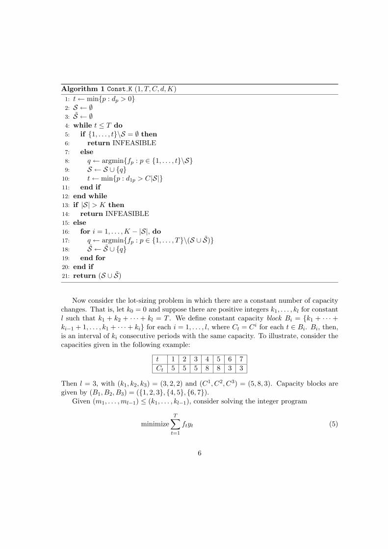
Algorithm 1 Const K (1, T, C, d, K)1: t← min{p : dp > 0}2: S ← ∅3: S ← ∅4: while t ≤ T do5: if {1, . . . , t}\S = ∅ then6: return INFEASIBLE7: else8: q ← argmin{fp : p ∈ {1, . . . , t}\S}9: S ← S ∪ {q}

10: t← min{p : d1p > C|S|}11: end if12: end while13: if |S| > K then14: return INFEASIBLE15: else16: for i = 1, . . . ,K − |S|, do17: q ← argmin{fp : p ∈ {1, . . . , T}\(S ∪ S)}18: S ← S ∪ {q}19: end for20: end if21: return (S ∪ S)

Now consider the lot-sizing problem in which there are a constant number of capacitychanges. That is, let k0 = 0 and suppose there are positive integers k1, . . . , kl for constantl such that k1 + k2 + · · · + kl = T . We define constant capacity block Bi = {k1 + · · · +ki−1 + 1, . . . , k1 + · · ·+ ki} for each i = 1, . . . , l, where Ct = Ci for each t ∈ Bi. Bi, then,is an interval of ki consecutive periods with the same capacity. To illustrate, consider thecapacities given in the following example:

t 1 2 3 4 5 6 7Ct 5 5 5 8 8 3 3

Then l = 3, with (k1, k2, k3) = (3, 2, 2) and (C1, C2, C3) = (5, 8, 3). Capacity blocks aregiven by (B1, B2, B3) = ({1, 2, 3}, {4, 5}, {6, 7}).

Given (m1, . . . ,ml−1) ≤ (k1, . . . , kl−1), consider solving the integer program

minimizeT∑

t=1

ftyt (5)

6

subject tot∑

j=1

Cjyj ≥ d1t t ∈ {1, ..., T} (6)

∑j∈Bi

yj = mi i = 1, . . . , l − 1 (7)

yt ∈ {0, 1} t ∈ {1, ..., T}. (8)

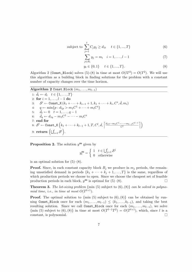
Algorithm 2 (Const_Block) solves (5)-(8) in time at most O(lT 2) = O(T 2). We will usethis algorithm as a building block in finding solutions for the problem with a constantnumber of capacity changes over the time horizon.

Algorithm 2 Const Block (m1, . . . ,ml−1)1: dt ← dt t ∈ {1, . . . , T}2: for i = 1, . . . , l − 1 do3: Si ← Const_K (k1 + · · ·+ ki−1 + 1, k1 + · · ·+ ki, C

i, d,mi)4: q ← min{p : d1p > m1C

1 + · · ·+ miCi}

5: dt ← 0 t = 1, . . . , q − 16: dq ← d1q −m1C

1 − · · · −miCi

7: end for8: S l ← Const_K

(k1 + · · ·+ kl−1 + 1, T, C l, d,

⌈d1T−m1C1−···−ml−1Cl−1

Cl

⌉)9: return

(⋃li=1 Si

).

Proposition 2. The solution ym given by

ymt =

{1 t ∈

⋃lj=1 Sj

0 otherwise

is an optimal solution for (5)–(8).

Proof. Since, in each constant capacity block Bj we produce in mj periods, the remain-ing unsatisfied demand in periods {k1 + · · · + kj + 1, . . . , T} is the same, regardless ofwhich production periods we choose to open. Since we choose the cheapest set of feasibleproduction periods in each block, ym is optimal for (5)–(8).

Theorem 3. The lot-sizing problem {min (5) subject to (6), (8)} can be solved in polyno-mial time, i.e., in time at most O(T l+1).

Proof. The optimal solution to {min (5) subject to (6), (8)} can be obtained by run-ning Const_Block once for each (m1, . . . ,ml−1) ≤ (k1, . . . , kl−1), and taking the bestresulting solution. Since we call Const_Block once for each (m1, . . . ,ml−1), we solve{min (5) subject to (6), (8)} in time at most O(T l−1T 2) = O(T l+1), which, since l is aconstant, is polynomial.

7

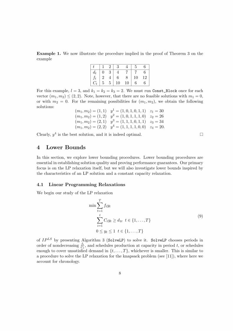
Example 1. We now illustrate the procedure implied in the proof of Theorem 3 on theexample

t 1 2 3 4 5 6dt 0 3 4 7 7 6ft 2 4 6 8 10 12Ct 5 5 10 10 6 6

For this example, l = 3, and k1 = k2 = k3 = 2. We must run Const_Block once for eachvector (m1,m2) ≤ (2, 2). Note, however, that there are no feasible solutions with m1 = 0,or with m2 = 0. For the remaining possibilities for (m1,m2), we obtain the followingsolutions:

(m1,m2) = (1, 1) y1 = (1, 0, 1, 0, 1, 1) z1 = 30(m1,m2) = (1, 2) y2 = (1, 0, 1, 1, 1, 0) z2 = 26(m1,m2) = (2, 1) y3 = (1, 1, 1, 0, 1, 1) z3 = 34(m1,m2) = (2, 2) y4 = (1, 1, 1, 1, 0, 0) z4 = 20.

Clearly, y4 is the best solution, and it is indeed optimal.

4 Lower Bounds

In this section, we explore lower bounding procedures. Lower bounding procedures areessential in establishing solution quality and proving performance guarantees. Our primaryfocus is on the LP relaxation itself, but we will also investigate lower bounds inspired bythe characteristics of an LP solution and a constant capacity relaxation.

4.1 Linear Programming Relaxations

We begin our study of the LP relaxation

minT∑

t=1

ftyt

t∑i=1

Ctyt ≥ d1t t ∈ {1, . . . , T}

0 ≤ yt ≤ 1 t ∈ {1, . . . , T}

(9)

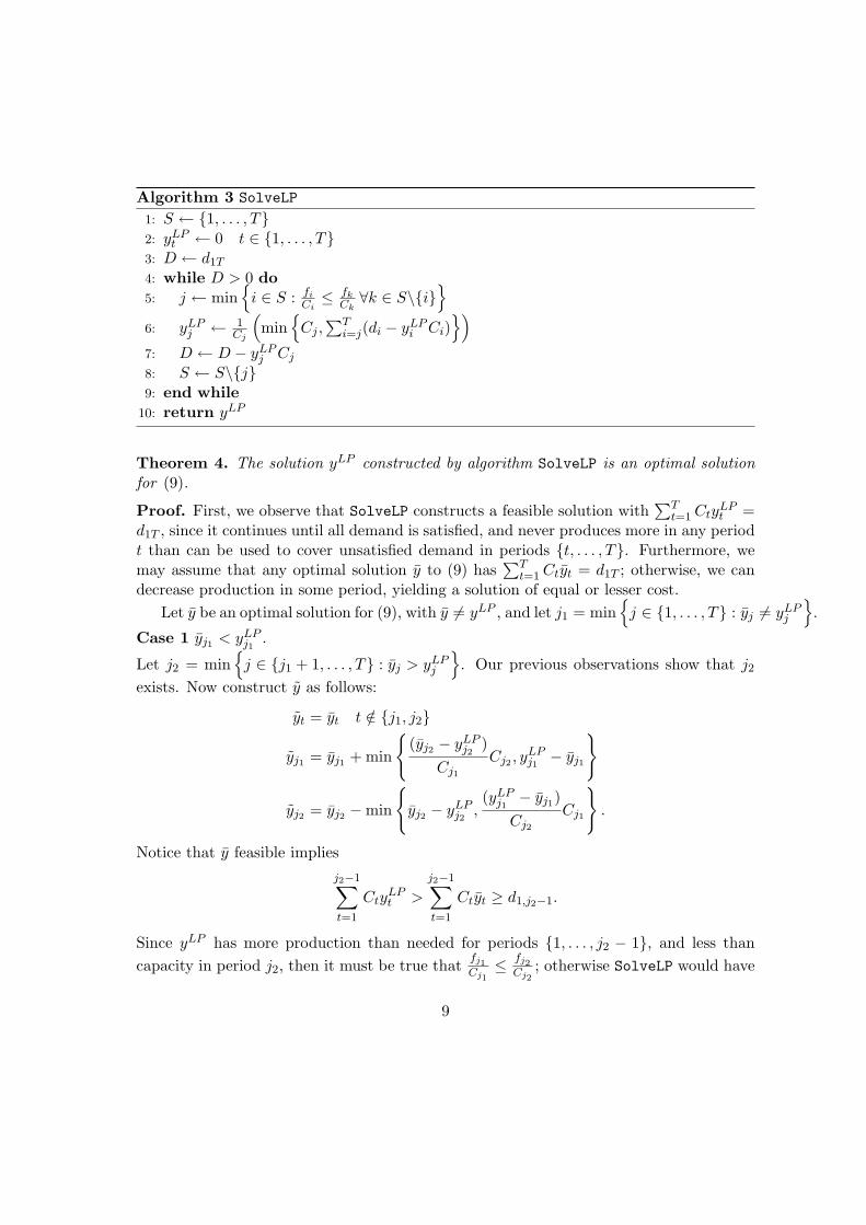
of IPLS by presenting Algorithm 3 (SolveLP) to solve it. SolveLP chooses periods inorder of nondecreasing ft

Ct, and schedules production at capacity in period t, or schedules

enough to cover unsatisfied demand in {t, . . . , T}, whichever is smaller. This is similar toa procedure to solve the LP relaxation for the knapsack problem (see [11]), where here weaccount for chronology.

8

Algorithm 3 SolveLP

1: S ← {1, . . . , T}2: yLP

t ← 0 t ∈ {1, . . . , T}3: D ← d1T

4: while D > 0 do5: j ← min

{i ∈ S : fi

Ci≤ fk

Ck∀k ∈ S\{i}

}6: yLP

j ← 1Cj

(min

{Cj ,∑T

i=j(di − yLPi Ci)

})7: D ← D − yLP

j Cj

8: S ← S\{j}9: end while

10: return yLP

Theorem 4. The solution yLP constructed by algorithm SolveLP is an optimal solutionfor (9).

Proof. First, we observe that SolveLP constructs a feasible solution with∑T

t=1 CtyLPt =

d1T , since it continues until all demand is satisfied, and never produces more in any periodt than can be used to cover unsatisfied demand in periods {t, . . . , T}. Furthermore, wemay assume that any optimal solution y to (9) has

∑Tt=1 Ctyt = d1T ; otherwise, we can

decrease production in some period, yielding a solution of equal or lesser cost.Let y be an optimal solution for (9), with y 6= yLP , and let j1 = min

{j ∈ {1, . . . , T} : yj 6= yLP

j

}.

Case 1 yj1 < yLPj1

.

Let j2 = min{

j ∈ {j1 + 1, . . . , T} : yj > yLPj

}. Our previous observations show that j2

exists. Now construct y as follows:

yt = yt t /∈ {j1, j2}

yj1 = yj1 + min

{(yj2 − yLP

j2)

Cj1

Cj2 , yLPj1 − yj1

}

yj2 = yj2 −min

{yj2 − yLP

j2 ,(yLP

j1− yj1)

Cj2

Cj1

}.

Notice that y feasible impliesj2−1∑t=1

CtyLPt >

j2−1∑t=1

Ctyt ≥ d1,j2−1.

Since yLP has more production than needed for periods {1, . . . , j2 − 1}, and less thancapacity in period j2, then it must be true that fj1

Cj1≤ fj2

Cj2; otherwise SolveLP would have

9

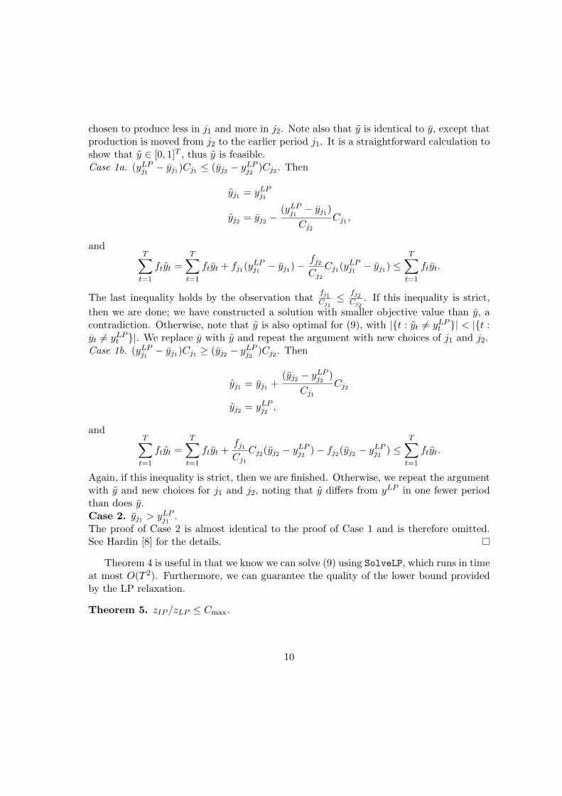
chosen to produce less in j1 and more in j2. Note also that y is identical to y, except thatproduction is moved from j2 to the earlier period j1. It is a straightforward calculation toshow that y ∈ [0, 1]T , thus y is feasible.Case 1a. (yLP

j1− yj1)Cj1 ≤ (yj2 − yLP

j2)Cj2 . Then

yj1 = yLPj1

yj2 = yj2 −(yLP

j1− yj1)

Cj2

Cj1 ,

andT∑

t=1

ftyt =T∑

t=1

ftyt + fj1(yLPj1 − yj1)−

fj2

Cj2

Cj1(yLPj1 − yj1) ≤

T∑t=1

ftyt.

The last inequality holds by the observation that fj1Cj1≤ fj2

Cj2. If this inequality is strict,

then we are done; we have constructed a solution with smaller objective value than y, acontradiction. Otherwise, note that y is also optimal for (9), with |{t : yt 6= yLP

t }| < |{t :yt 6= yLP

t }|. We replace y with y and repeat the argument with new choices of j1 and j2.Case 1b. (yLP

j1− yj1)Cj1 ≥ (yj2 − yLP

j2)Cj2 . Then

yj1 = yj1 +(yj2 − yLP

j2)

Cj1

Cj2

yj2 = yLPj2 ,

andT∑

t=1

ftyt =T∑

t=1

ftyt +fj1

Cj1

Cj2(yj2 − yLPj2 )− fj2(yj2 − yLP

j2 ) ≤T∑

t=1

ftyt.

Again, if this inequality is strict, then we are finished. Otherwise, we repeat the argumentwith y and new choices for j1 and j2, noting that y differs from yLP in one fewer periodthan does y.Case 2. yj1 > yLP

j1.

The proof of Case 2 is almost identical to the proof of Case 1 and is therefore omitted.See Hardin [8] for the details.

Theorem 4 is useful in that we know we can solve (9) using SolveLP, which runs in timeat most O(T 2). Furthermore, we can guarantee the quality of the lower bound providedby the LP relaxation.

Theorem 5. zIP /zLP ≤ Cmax.

10

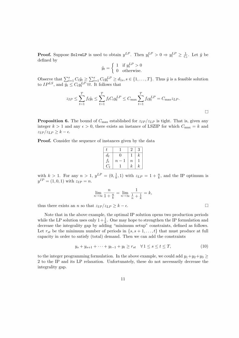
Proof. Suppose SolveLP is used to obtain yLP . Then yLPt > 0 ⇒ yLP

t ≥ 1Ct

. Let y bedefined by

yt ={

1 if yLPt > 0

0 otherwise.

Observe that∑s

t=1 Ctyt ≥∑s

t=1 CtyLPt ≥ d1s, s ∈ {1, . . . , T}. Thus y is a feasible solution

to IPLS , and yt ≤ CtyLPt ∀t. It follows that

zIP ≤T∑

t=1

ftyt ≤T∑

t=1

ftCtyLPt ≤ Cmax

T∑t=1

ftyLPt = CmaxzLP .

Proposition 6. The bound of Cmax established for zIP /zLP is tight. That is, given anyinteger k > 1 and any ε > 0, there exists an instance of LSZIP for which Cmax = k andzIP /zLP ≥ k − ε.

Proof. Consider the sequence of instances given by the data

t 1 2 3dt 0 1 kft n− 1 n 1Ct 1 k k

with k > 1. For any n > 1, yLP = (0, 1k , 1) with zLP = 1 + n

k , and the IP optimum isyIP = (1, 0, 1) with zIP = n.

limn→∞

n

1 + nk

= limn→∞

11n + 1

k

= k,

thus there exists an n so that zIP /zLP ≥ k − ε.

Note that in the above example, the optimal IP solution opens two production periodswhile the LP solution uses only 1+ 1

k . One may hope to strengthen the IP formulation anddecrease the integrality gap by adding “minimum setup” constraints, defined as follows.Let rst be the minimum number of periods in {s, s + 1, . . . , t} that must produce at fullcapacity in order to satisfy (total) demand. Then we can add the constraints

ys + ys+1 + · · ·+ yt−1 + yt ≥ rst ∀ 1 ≤ s ≤ t ≤ T, (10)

to the integer programming formulation. In the above example, we could add y1+y2+y3 ≥2 to the IP and its LP relaxation. Unfortunately, these do not necessarily decrease theintegrality gap.

11

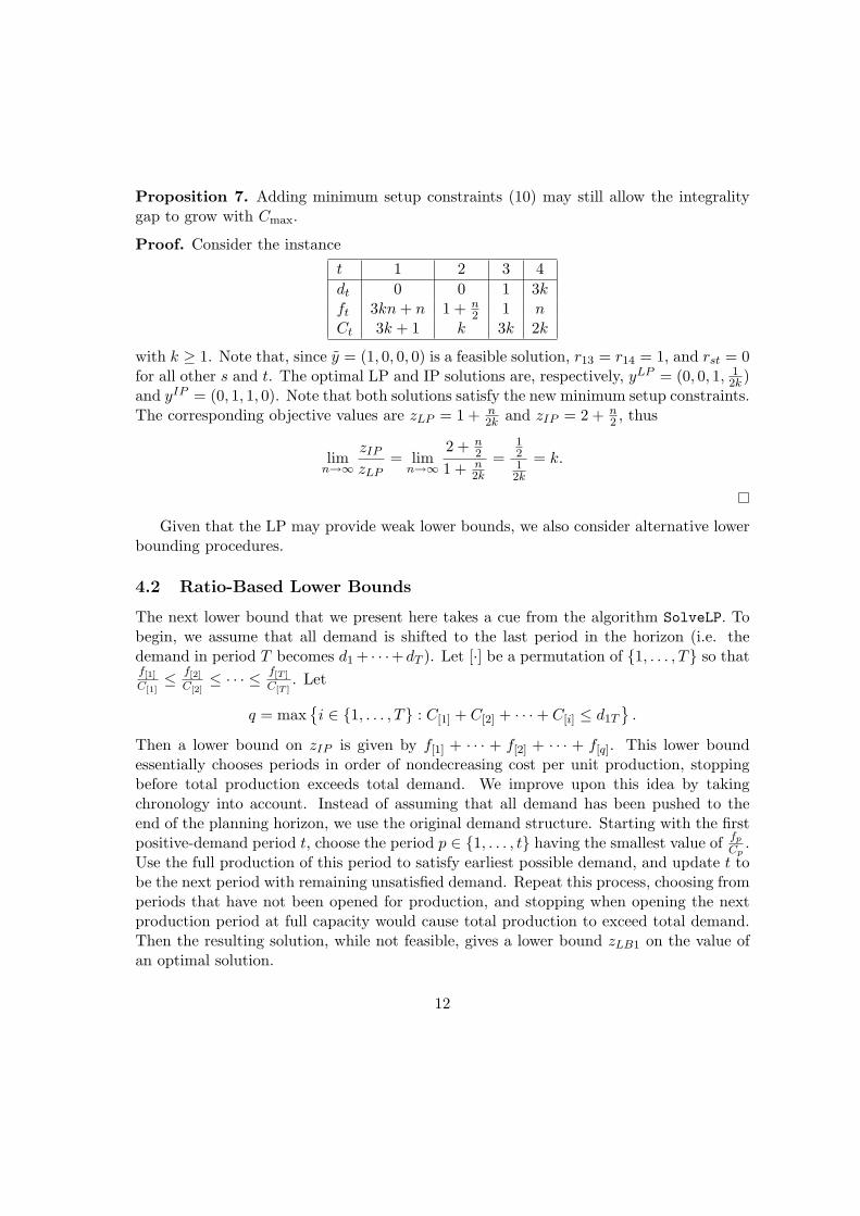
Proposition 7. Adding minimum setup constraints (10) may still allow the integralitygap to grow with Cmax.

Proof. Consider the instance

t 1 2 3 4dt 0 0 1 3kft 3kn + n 1 + n

2 1 nCt 3k + 1 k 3k 2k

with k ≥ 1. Note that, since y = (1, 0, 0, 0) is a feasible solution, r13 = r14 = 1, and rst = 0for all other s and t. The optimal LP and IP solutions are, respectively, yLP = (0, 0, 1, 1

2k )and yIP = (0, 1, 1, 0). Note that both solutions satisfy the new minimum setup constraints.The corresponding objective values are zLP = 1 + n

2k and zIP = 2 + n2 , thus

limn→∞

zIP

zLP= lim

n→∞

2 + n2

1 + n2k

=1212k

= k.

Given that the LP may provide weak lower bounds, we also consider alternative lowerbounding procedures.

4.2 Ratio-Based Lower Bounds

The next lower bound that we present here takes a cue from the algorithm SolveLP. Tobegin, we assume that all demand is shifted to the last period in the horizon (i.e. thedemand in period T becomes d1 + · · ·+dT ). Let [·] be a permutation of {1, . . . , T} so thatf[1]

C[1]≤ f[2]

C[2]≤ · · · ≤ f[T ]

C[T ]. Let

q = max{i ∈ {1, . . . , T} : C[1] + C[2] + · · ·+ C[i] ≤ d1T

}.

Then a lower bound on zIP is given by f[1] + · · · + f[2] + · · · + f[q]. This lower boundessentially chooses periods in order of nondecreasing cost per unit production, stoppingbefore total production exceeds total demand. We improve upon this idea by takingchronology into account. Instead of assuming that all demand has been pushed to theend of the planning horizon, we use the original demand structure. Starting with the firstpositive-demand period t, choose the period p ∈ {1, . . . , t} having the smallest value of fp

Cp.

Use the full production of this period to satisfy earliest possible demand, and update t tobe the next period with remaining unsatisfied demand. Repeat this process, choosing fromperiods that have not been opened for production, and stopping when opening the nextproduction period at full capacity would cause total production to exceed total demand.Then the resulting solution, while not feasible, gives a lower bound zLB1 on the value ofan optimal solution.

12

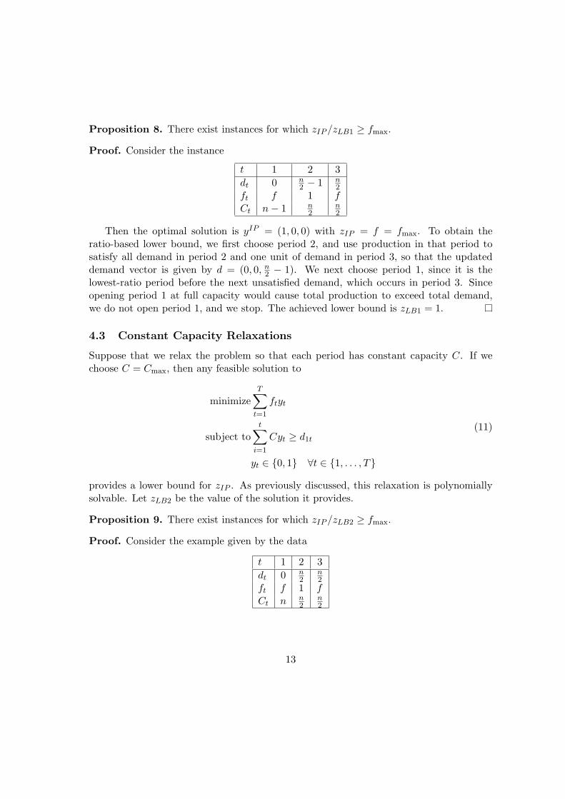
Proposition 8. There exist instances for which zIP /zLB1 ≥ fmax.

Proof. Consider the instance

t 1 2 3dt 0 n

2 − 1 n2

ft f 1 fCt n− 1 n

2n2

Then the optimal solution is yIP = (1, 0, 0) with zIP = f = fmax. To obtain theratio-based lower bound, we first choose period 2, and use production in that period tosatisfy all demand in period 2 and one unit of demand in period 3, so that the updateddemand vector is given by d = (0, 0, n

2 − 1). We next choose period 1, since it is thelowest-ratio period before the next unsatisfied demand, which occurs in period 3. Sinceopening period 1 at full capacity would cause total production to exceed total demand,we do not open period 1, and we stop. The achieved lower bound is zLB1 = 1.

4.3 Constant Capacity Relaxations

Suppose that we relax the problem so that each period has constant capacity C. If wechoose C = Cmax, then any feasible solution to

minimizeT∑

t=1

ftyt

subject tot∑

i=1

Cyt ≥ d1t

yt ∈ {0, 1} ∀t ∈ {1, . . . , T}

(11)

provides a lower bound for zIP . As previously discussed, this relaxation is polynomiallysolvable. Let zLB2 be the value of the solution it provides.

Proposition 9. There exist instances for which zIP /zLB2 ≥ fmax.

Proof. Consider the example given by the data

t 1 2 3dt 0 n

2n2

ft f 1 fCt n n

2n2

13

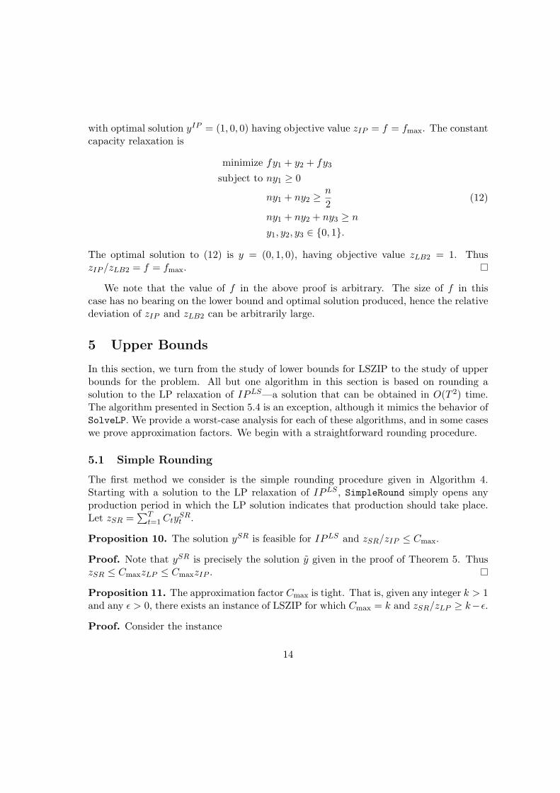
with optimal solution yIP = (1, 0, 0) having objective value zIP = f = fmax. The constantcapacity relaxation is

minimize fy1 + y2 + fy3

subject to ny1 ≥ 0

ny1 + ny2 ≥n

2ny1 + ny2 + ny3 ≥ n

y1, y2, y3 ∈ {0, 1}.

(12)

The optimal solution to (12) is y = (0, 1, 0), having objective value zLB2 = 1. ThuszIP /zLB2 = f = fmax.

We note that the value of f in the above proof is arbitrary. The size of f in thiscase has no bearing on the lower bound and optimal solution produced, hence the relativedeviation of zIP and zLB2 can be arbitrarily large.

5 Upper Bounds

In this section, we turn from the study of lower bounds for LSZIP to the study of upperbounds for the problem. All but one algorithm in this section is based on rounding asolution to the LP relaxation of IPLS—a solution that can be obtained in O(T 2) time.The algorithm presented in Section 5.4 is an exception, although it mimics the behavior ofSolveLP. We provide a worst-case analysis for each of these algorithms, and in some caseswe prove approximation factors. We begin with a straightforward rounding procedure.

5.1 Simple Rounding

The first method we consider is the simple rounding procedure given in Algorithm 4.Starting with a solution to the LP relaxation of IPLS , SimpleRound simply opens anyproduction period in which the LP solution indicates that production should take place.Let zSR =

∑Tt=1 Cty

SRt .

Proposition 10. The solution ySR is feasible for IPLS and zSR/zIP ≤ Cmax.

Proof. Note that ySR is precisely the solution y given in the proof of Theorem 5. ThuszSR ≤ CmaxzLP ≤ CmaxzIP .

Proposition 11. The approximation factor Cmax is tight. That is, given any integer k > 1and any ε > 0, there exists an instance of LSZIP for which Cmax = k and zSR/zLP ≥ k−ε.

Proof. Consider the instance

14

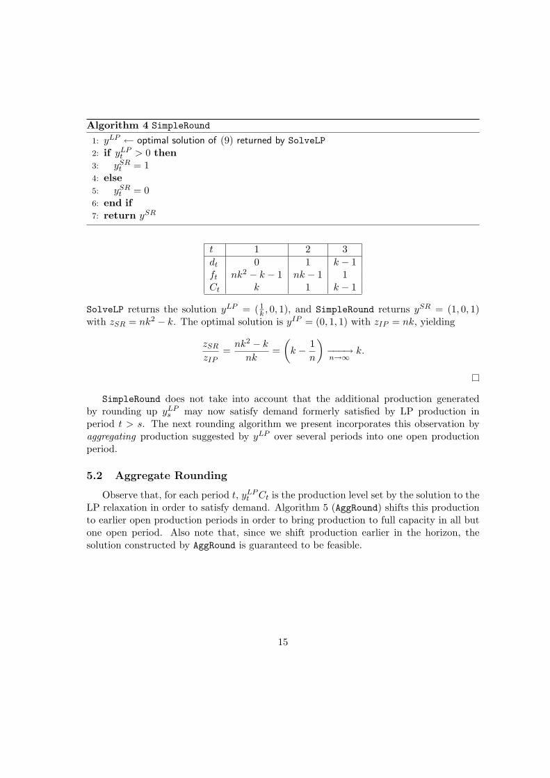
Algorithm 4 SimpleRound

1: yLP ← optimal solution of (9) returned by SolveLP2: if yLP

t > 0 then3: ySR

t = 14: else5: ySR

t = 06: end if7: return ySR

t 1 2 3dt 0 1 k − 1ft nk2 − k − 1 nk − 1 1Ct k 1 k − 1

SolveLP returns the solution yLP = ( 1k , 0, 1), and SimpleRound returns ySR = (1, 0, 1)

with zSR = nk2 − k. The optimal solution is yIP = (0, 1, 1) with zIP = nk, yielding

zSR

zIP=

nk2 − k

nk=(

k − 1n

)−−−→n→∞

k.

SimpleRound does not take into account that the additional production generatedby rounding up yLP

s may now satisfy demand formerly satisfied by LP production inperiod t > s. The next rounding algorithm we present incorporates this observation byaggregating production suggested by yLP over several periods into one open productionperiod.

5.2 Aggregate Rounding

Observe that, for each period t, yLPt Ct is the production level set by the solution to the

LP relaxation in order to satisfy demand. Algorithm 5 (AggRound) shifts this productionto earlier open production periods in order to bring production to full capacity in all butone open period. Also note that, since we shift production earlier in the horizon, thesolution constructed by AggRound is guaranteed to be feasible.

15

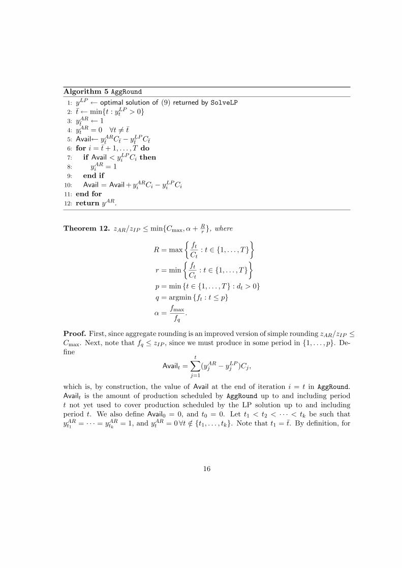
Algorithm 5 AggRound

1: yLP ← optimal solution of (9) returned by SolveLP2: t← min{t : yLP

t > 0}3: yAR

t ← 14: yAR

t = 0 ∀t 6= t5: Avail← yAR

t Ct − yLPt Ct

6: for i = t + 1, . . . , T do7: if Avail < yLP

i Ci then8: yAR

i = 19: end if

10: Avail = Avail + yARi Ci − yLP

i Ci

11: end for12: return yAR.

Theorem 12. zAR/zIP ≤ min{Cmax, α + Rr }, where

R = max{

ft

Ct: t ∈ {1, . . . , T}

}r = min

{ft

Ct: t ∈ {1, . . . , T}

}p = min {t ∈ {1, . . . , T} : dt > 0}q = argmin {ft : t ≤ p}

α =fmax

fq.

Proof. First, since aggregate rounding is an improved version of simple rounding zAR/zIP ≤Cmax. Next, note that fq ≤ zIP , since we must produce in some period in {1, . . . , p}. De-fine

Availt =t∑

j=1

(yARj − yLP

j )Cj ,

which is, by construction, the value of Avail at the end of iteration i = t in AggRound.Availt is the amount of production scheduled by AggRound up to and including periodt not yet used to cover production scheduled by the LP solution up to and includingperiod t. We also define Avail0 = 0, and t0 = 0. Let t1 < t2 < · · · < tk be such thatyAR

t1 = · · · = yARtk

= 1, and yARt = 0∀t /∈ {t1, . . . , tk}. Note that t1 = t. By definition, for

16

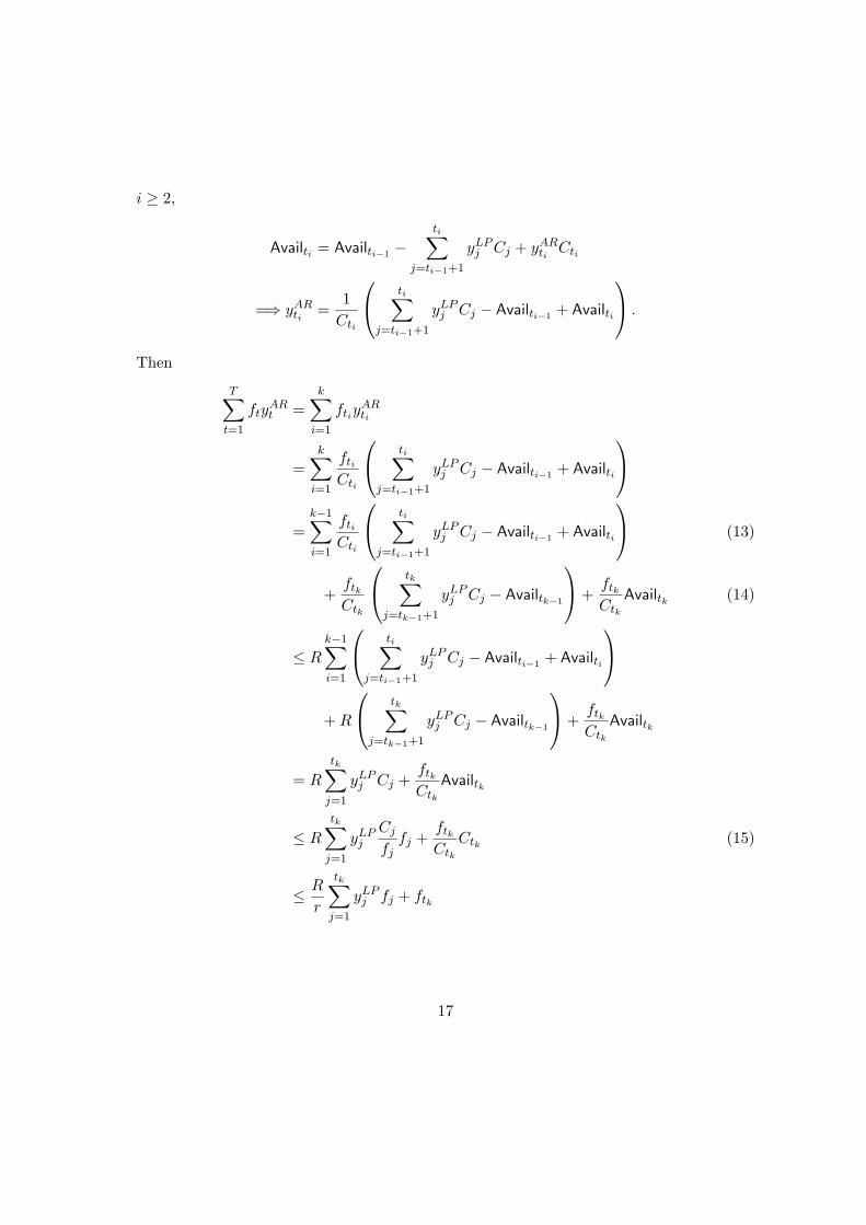
i ≥ 2,

Availti = Availti−1 −ti∑

j=ti−1+1

yLPj Cj + yAR

ti Cti

=⇒ yARti =

1Cti

ti∑j=ti−1+1

yLPj Cj − Availti−1 + Availti

.

Then

T∑t=1

ftyARt =

k∑i=1

ftiyARti

=k∑

i=1

fti

Cti

ti∑j=ti−1+1

yLPj Cj − Availti−1 + Availti

=

k−1∑i=1

fti

Cti

ti∑j=ti−1+1

yLPj Cj − Availti−1 + Availti

(13)

+ftk

Ctk

tk∑j=tk−1+1

yLPj Cj − Availtk−1

+ftk

Ctk

Availtk (14)

≤ Rk−1∑i=1

ti∑j=ti−1+1

yLPj Cj − Availti−1 + Availti

+ R

tk∑j=tk−1+1

yLPj Cj − Availtk−1

+ftk

Ctk

Availtk

= R

tk∑j=1

yLPj Cj +

ftk

Ctk

Availtk

≤ R

tk∑j=1

yLPj

Cj

fjfj +

ftk

Ctk

Ctk (15)

≤ R

r

tk∑j=1

yLPj fj + ftk

17

≤ R

r

T∑j=1

yIPj fj +

fmax

fqfq

≤(

R

r+ α

)zIP .

The parenthetical term in (13) equals yARti Cti and is therefore nonnegative. As AggRound

chooses to produce in period tk, Availtk−1is insufficient to satisfy LP production in periods

tk−1 + 1, . . . , tk and therefore the parenthetical term in (14) is also nonnegative. At thesame time, this implies that Availtk ≤ Ctk (because some of the capacity of period tkmust be used to satisfy LP production in that period) hence inequality (15) holds. Thiscompletes the proof.

Proposition 13. The approximation factor Cmax is tight. That is, given any integer k > 1and any ε > 0, there exists an instance of LSZIP for which Cmax = k and zAR/zLP ≥ k−ε.

Proof. Consider the instance used in the proof of Proposition 11. Algorithm AggRoundreturns yAR = (1, 0, 0) with zAR = nk2 − k − 1. The optimal solution is yIP = (0, 1, 1)with zIP = nk.

zAR

zIP=

nk2 − k − 1nk

=(

k − 1n− 1

nk

)−−−→n→∞

k.

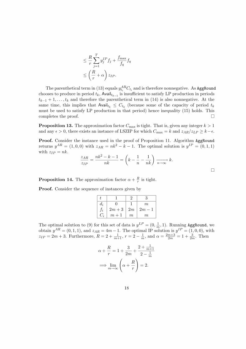
Proposition 14. The approximation factor α + Rr is tight.

Proof. Consider the sequence of instances given by

t 1 2 3di 0 1 mfi 2m + 3 2m 2m− 1Ci m + 1 m m

The optimal solution to (9) for this set of data is yLP = (0, 1m , 1). Running AggRound, we

obtain yAR = (0, 1, 1), and zAR = 4m− 1. The optimal IP solution is yIP = (1, 0, 0), withzIP = 2m + 3. Furthermore, R = 2 + 1

m+1 , r = 2− 1m , and α = 2m+3

2m = 1 + 32m . Then

α +R

r= 1 +

32m

+2 + 1

m+1

2− 1m

=⇒ limm→∞

(α +

R

r

)= 2.

18

Observe that α + Rr < Cmax. Moreover,

zAR/zIP =4m− 12m + 3

=4− 1

m

2 + 3m

=⇒ limm→∞

zAR/zIP = 2.

Observe that in this example AggRound and SimpleRound produce the same solution,and in this case the solution is minimal (closing any open production period creates aninfeasible solution).

5.3 Greedy Rounding

GreedyRound, as its name suggests, selects production periods greedily, using the solutionto the LP relaxation as a guide. It selects the earliest period p with positive production inthe LP solution. It then finds the cheapest period in which it can produce at least Cpy

LPp

before that production is actually needed to satisfy demand. This production is used tosatisfy demand and to replace production in the LP solution. GreedyRound repeats thisprocess until all demand is satisfied. We present a formal description of GreedyRound inAlgorithm 6.

Proposition 15. zGR/zIP ≤ Cmax.

Proof. GreedyRound considers each period t with positive production (say p units) in theLP. It then tries to find a period with capacity at least p before the next positive demand,but that has lower setup cost than period t. Therefore, GreedyRound is no worse thanSimpleRound, so it must have a performance guarantee of Cmax.

Proposition 16. There exist instances for which Cmax is tight.

Proof. To establish this result, we examine the sequence of instances in which T = 2n+1and

d2i−1 = 0 C2i−1 = 1 f2i = 2(n− i + 2) i = 1, . . . , n

d2i = 1 C2i = 2 f2i+1 = 2(n− i) + 1 i = 1, . . . , n

d2n+1 = 1 C2n+1 = 1 f1 = n + 2

19

Algorithm 6 GreedyRound

1: S ← ∅2: yLP ← optimal solution to (9) returned by SolveLP3: dt ← dt t ∈ {1, . . . , T}4: while

∑Tt=1 yLP

t > 0 and∑T

t=1 dt > 0 do5: p← min{t : yLP

t > 0}6: s← min{t : dt > 0}7: q ← argmin{t ∈ {1, . . . , s}\S and Ct ≥ Cpy

LPp : ft}

8: S ← S ∪ {q}9: A← Cq, B ← Cq

10: while A > 0 and p ≤ T do11: yLP

p ← 1Cp

(CpyLPp −min{A,Cpy

LPp })

12: A← A−min{A,CpyLPp }

13: p← p + 114: end while15: while B > 0 and s ≤ T do16: ds ← ds −min{B, ds}17: B ← B −min{B, ds}18: s← s + 119: end while20: end while21: return S

The solutions yLP given by SolveLP and yGR given by GreedyRound are given by

yLP2i =

12

i = 1, . . . , n yGR2i = 0 i = 0, . . . , n

yLP2i+1 = 0 i = 0, . . . , n− 1 yGR

2i+1 = 1 i = 1, . . . , n

yLP2n+1 = 1

with zGR = n2 + n + 2. The optimal solution to IPLS is given by yIP2(2i+1) = 1, i =

0, . . . , n2 − 1, yIP

2n+1 = 1, and yIPi = 0 otherwise, with zIP = n2

2 + 2n + 1. Then

limn→∞

zGR

zIP= lim

n→∞

n2 + n + 2n2

2 + 2n + 1= lim

n→∞

1 + 1n + 2

n2

12 + 2

n + 1n2

= 2.

Proposition 17. There exist instances for which zGR/zIP grows with Cmax.

Proof. Consider the instance

20

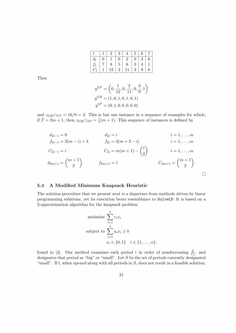
t 1 2 3 4 5 6 7dt 0 1 0 2 0 3 6ft 7 8 5 6 3 4 1Ct 1 12 2 11 3 9 6

Then

yLP =(

0,112

, 0,211

, 0,39, 1)

yGR = (1, 0, 1, 0, 1, 0, 1)

yIP = (0, 1, 0, 0, 0, 0, 0)

and zGR/zIP = 16/8 = 2. This is but one instance in a sequence of examples for which,if T = 2m + 1, then zGR/zIP = 1

2(m + 1). This sequence of instances is defined by

d2i−1 = 0 d2i = i i = 1, . . . ,m

f2i−1 = 2(m− i) + 3 f2i = 2(m + 2− i) i = 1, . . . ,m

C2i−1 = i C2i = m(m + 1)−(

i

2

)i = 1, . . . ,m

d2m+1 =(

m + 12

)f2m+1 = 1 C2m+1 =

(m + 1

2

).

5.4 A Modified Minimum Knapsack Heuristic

The solution procedure that we present next is a departure from methods driven by linearprogramming solutions, yet its execution bears resemblance to SolveLP. It is based on a2-approximation algorithm for the knapsack problem

minimizen∑

i=1

cixi

subject ton∑

i=1

aixi ≥ b

xi ∈ {0, 1} i ∈ {1, . . . , n}.

found in [4]. Our method examines each period t in order of nondecreasing ft

Ct, and

designates that period as “big” or “small”. Let S be the set of periods currently designated“small”. If t, when opened along with all periods in S, does not result in a feasible solution,

21

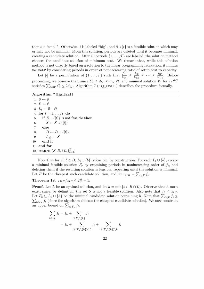
then t is “small”. Otherwise, t is labeled “big”, and S∪{t} is a feasible solution which mayor may not be minimal. From this solution, periods are deleted until it becomes minimal,creating a candidate solution. After all periods {1, . . . , T} are labeled, the solution methodchooses the candidate solution of minimum cost. We remark that, while this solutionmethod is not directly based on a solution to the linear programming relaxation, it mimicsSolveLP by considering periods in order of nondecreasing ratio of setup cost to capacity.

Let [·] be a permutation of {1, . . . , T} such that f[1]

C[1]≤ f[2]

C[2]≤ · · · ≤ f[T ]

C[T ]. Before

proceeding, we observe that, since Ct ≤ dtT ≤ d1T ∀t, any minimal solution W for IPLS

satisfies∑

t∈W Ct ≤ 2d1T . Algorithm 7 (Big_Small) describes the procedure formally.

Algorithm 7 Big Small

1: S ← ∅2: B ← ∅3: Lt ← ∅ ∀t4: for t = 1, . . . , T do5: if S ∪ {[t]} is not feasible then6: S ← S ∪ {[t]}7: else8: B ← B ∪ {[t]}9: L[t] ← S

10: end if11: end for12: return (S, B, {Lt}Tt=1)

Note that for all b ∈ B, Lb ∪ {b} is feasible, by construction. For each Lb ∪ {b}, createa minimal feasible solution Fb by examining periods in nonincreasing order of ft, anddeleting them if the resulting solution is feasible, repeating until the solution is minimal.Let F be the cheapest such candidate solution, and let zMK =

∑t∈F ft.

Theorem 18. zMK/zIP ≤ 2Rr + 1.

Proof. Let L be an optimal solution, and let h = min{t ∈ B ∩ L}. Observe that h mustexist, since, by definition, the set S is not a feasible solution. Also note that fh ≤ zIP .Let Fh ⊆ Lh ∪ {h} be the minimal candidate solution containing h. Note that

∑t∈F ft ≤∑

t∈Fhft (since the algorithm chooses the cheapest candidate solution). We now construct

an upper bound on∑

t∈Fhft.∑

t∈Fh

ft = fh +∑

t∈Fh\{h}

ft

= fh +∑

t∈(Fh\{h})∩L

ft +∑

t∈(Fh\{h})\L

ft

22

≤ fh +∑

t∈(Fh\{h})∩L

ft +∑

t∈(Fh\{h})\L

fh

ChCt (16)

≤ fh +∑

t∈(Fh\{h})∩L

ft +fh

Ch

2d1T −∑

t∈(Fh\{h})∩L

Ct

(17)

≤ fh +∑

t∈(Fh\{h})∩L

ft +fh

Ch

∑t∈L\(Fh\{h})

Ct +fh

Chd1T (18)

≤ fh +R

r

∑t∈(Fh\{h})∩L

ft +fh

Ch

∑t∈L\(Fh\{h})

Ctft

ft+

fh

Ch

∑t∈L

Ctft

ft

≤ fh +R

r

∑t∈L

ft +R

r

∑t∈L

ft

≤(

2R

r+ 1)

zIP .

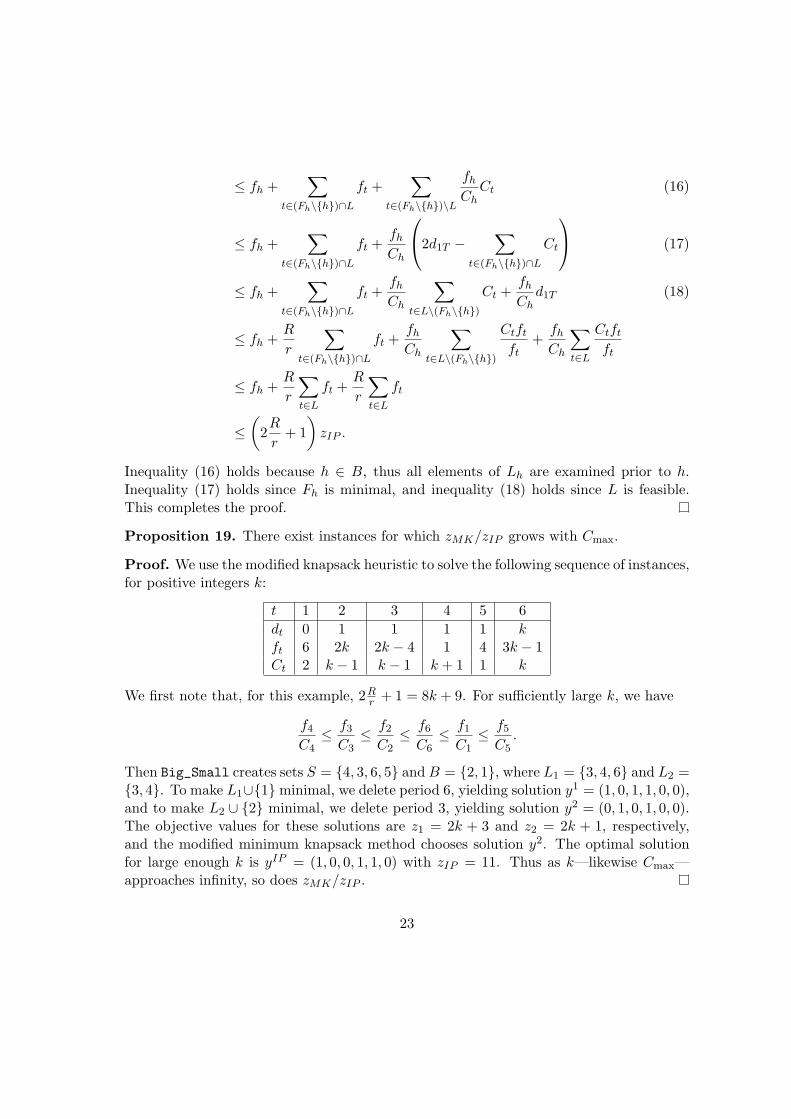
Inequality (16) holds because h ∈ B, thus all elements of Lh are examined prior to h.Inequality (17) holds since Fh is minimal, and inequality (18) holds since L is feasible.This completes the proof.

Proposition 19. There exist instances for which zMK/zIP grows with Cmax.

Proof. We use the modified knapsack heuristic to solve the following sequence of instances,for positive integers k:

t 1 2 3 4 5 6dt 0 1 1 1 1 kft 6 2k 2k − 4 1 4 3k − 1Ct 2 k − 1 k − 1 k + 1 1 k

We first note that, for this example, 2Rr + 1 = 8k + 9. For sufficiently large k, we have

f4

C4≤ f3

C3≤ f2

C2≤ f6

C6≤ f1

C1≤ f5

C5.

Then Big_Small creates sets S = {4, 3, 6, 5} and B = {2, 1}, where L1 = {3, 4, 6} and L2 ={3, 4}. To make L1∪{1}minimal, we delete period 6, yielding solution y1 = (1, 0, 1, 1, 0, 0),and to make L2 ∪ {2} minimal, we delete period 3, yielding solution y2 = (0, 1, 0, 1, 0, 0).The objective values for these solutions are z1 = 2k + 3 and z2 = 2k + 1, respectively,and the modified minimum knapsack method chooses solution y2. The optimal solutionfor large enough k is yIP = (1, 0, 0, 1, 1, 0) with zIP = 11. Thus as k—likewise Cmax—approaches infinity, so does zMK/zIP .

23

6 Future Research

We have analyzed a variety of fast algorithms for a core variant of the single-item lot-sizingproblem. All these algorithms are based, either directly or indirectly, on the solution ofthe LP relaxation of the natural formulation of the problem. For each algorithm, we haveproved a data dependent performance guarantee, typically dependent on the maximumcapacity Cmax and have shown that these performance guarantees are tight. These re-sults suggest that it will be difficult, if not impossible, to derive LP-based approximationalgorithms with a constant performance guarantee. However, we have to realize that wehave carried out a worst-case analysis and that it may well be the case that in practicethe bounds produced by the algorithms proposed are quite good. We plan to carry outan empirical study to establish the practical performance of our algorithms in the nearfuture.

24

References

[1] Bar-Noy, A., Guha, S., Naor, J., & Schieber, B. (2001). Approximating the Through-put of Multiple Machines in Real-Time Scheduling. SIAM Journal on Computing 31,331-352.

[2] Bitran, G. & Yanasse, H. (1982). Computational Complexity of the Capacitated LotSize Problem. Management Science 29, 1174–1186.

[3] Chen, H.-D. & Lee, C.-Y. (1994). A New Dynamic Programming Algorithm for theSingle Item Capacitated Dynamic Lot-size model. Journal of Global Optimization 4,285-300.

[4] Csirik, J., Frenk, J., Labbe, M., & Zhang, S. (1991). Heuristics for the 0-1 Min-Knapsack Problem. Acta Cybernetica 10, 15–20.

[5] Florian, M. & Klein, M. (1971). Deterministic Production Planning with ConcaveCosts and Capacity Constraints. Management Science 18, 12–20.

[6] Goemans, M.X., Queyranne, M., Schulz, A.S., Skutella, M., & Wang, Y. (2002). Sin-gle Machine Scheduling with Release Dates. SIAM Journal on Discrete Mathematics15, 165-192.

[7] Hall, L.A., Schulz, A.S., Shmoys, D.B., & Wein, J. (1997). Scheduling to MinimizeAverage Completion Time: Off-line and On-line Approximation Algorithms. Mathe-matics of Operations Research 22, 513-544.

[8] Hardin, J.R. (2001). Resource-constrained Scheduling and Production Planning: Lin-ear Programming-based Studies. PhD thesis, Georgia Institute of Technology.

[9] Leung, J., Magnanti, T., & Vachani, R. (1989). Facets and Algorithms for CapacitatedLot-Sizing. Mathematical Programming 45, 331–359.

[10] Miller, A. (1999). Polyhedral Approaches to Capacitated Lot-Sizing Problems. PhDthesis, Georgia Institute of Technology.

[11] Nemhauser, G. & Wolsey, L. (1988). Integer and Combinatorial Optimization. NewYork: Wiley.

[12] Pochet, Y. (1988). Valid Inequalities and Separation for Capacitated Economic Lot-Sizing. Operations Research Letters 7, 109–116.

[13] Pochet, Y. & Wolsey, L. (1994). Polyhedra for Lot-Sizing with Wagner-Whitin Costs.Mathematical Programming 67, 297–323.

25

[14] Savelsbergh, M., Uma, R., & Wein, J. (2005). An Experimental Study of LP-BasedApproximation Algorithms for Scheduling Problems. INFORMS Journal on Com-puting 17, 123-134.

[15] Schulz, A.S. & Skutella, M. (2002). Scheduling Unrelated Machines by RandomizedRounding. SIAM Journal of Discrete Mathematics 15, 450-469.

[16] Van Hoesel, C. & Wagelmans, A. (1996). An O(T 3) Algorithm for the EconomicLot-Sizing Problem with Constant Capacities. Management Science 42, 142-150.

[17] Van Hoesel, C. & Wagelmans, A. (2001). Fully polynomial approximation schemesfor single-item capacitated economic lot-sizing problems. Mathematics of OperationsResearch 26, 339–357.

[18] Vazirani, V. (2001). Approximation Algorithms. New York: Springer.

[19] Wagner, H. & Whitin, T. (1958). A Dynamic Version of the Economic Lot SizeModel. Management Science 5, 89–96.

26