Lead Time Considerations for the Multi-Level Capacitated

Lot-sizing Problem∗

Christian Almedera,c, Diego Klabjanb, Bernardo Almada-Loboc

August 26, 2009

aUniversity of Vienna, Faculty of Economics, Business and Statistics, Brünnerstr. 72, A-1210

Vienna, Austria.b Department of Industrial Engineering and Management Sciences, Northwestern University,

2145 Sheridan Road, Tech M239 Evanston, IL 60208-3119, USA.cFaculdade de Engenharia da Universidade do Porto, Rua Dr. Roberto Frias s/n, Porto

4200-465, Portugal.

Abstract

The classical multi-level capacitated lot-sizing problem is often not suitable to correctly

capture resource requirements and precedence relations. We tackle this issue by explicitly

modeling these two aspects. Two models are presented; one considering batch production

and the other one allowing lot-streaming. Comparisons with traditional models demonstrate

the capability of the new approach to deliver more realistic and practically feasible results.

Large-scale cases are solved by Benders, which has been enhanced in several novel ways.

Keywords: Lot-sizing, Scheduling, Mathematical Programming, Optimization

Mathematics Subject Classi�cation: 90B30, 90C11

1 Introduction

Extensive work has been reported in tackling the multi-level capacitated lot-sizing problem (ML-

CLSP), which lies at the core of many production planning systems. Numerous models and

solution approaches to support MLCLSP have been practically integrated with Manufacturing

Resource Planning, Master Production Scheduling or Enterprize Resource Planning systems.

MLCLSP �ts the highest level of planning in one of the most prominent hierarchical systems,

namely two-level production planning and scheduling. In fact, the complexity of the product

structure (bill-of-materials or BOM) of real-world cases has motivated researchers to decompose

hierarchically the overall planning system into a set of more manageable subsystems. At the

upper level of two-level production planning and scheduling, the tactical driver is to determine

the amount of each product that must be produced in each time-period across several resources

(sizing of lots). The production scheduling (sequencing of lots) is left to the lower operational

level of planning. In order to ensure that the plans generated at the upper-level can be scheduled

∗This research has been supported, in part, by Grant # J2815-N13 from the Austrian Science Foundation.

1

afterwards, the interdependencies between both levels should be incorporated in the solution

approaches, through top-down and bottom-up in�uences.

The majority of the models and algorithms proposed for MLCLSP rely on one of the following

two assumptions: either lead times are neglected, thus allowing predecessors and successors

to be produced in the same period; or lead times account for at least one period for each

component, forcing the throughput time (in number of periods) of the �nished products to be at

least equal to the number of levels of the BOM. Buschkühl et al. (2008) report in their review

that out of 16 papers dealing with metaheuristic solutions to MLCLSP, only one methodology

considers lead time, while all others neglect it. The present work is motivated by the observation

that the majority of the solutions published for well-known MLCLSP instances su�er from this

assumption. Indeed, the zero lead time assumption leads to plans that are not implementable,

as the lower-level scheduling problem is likely to be infeasible. This is more pronounced as the

capacity tightens. On the other hand, positive lead time usually results in huge amounts of

work-in-process, which tends to increase with a larger number of levels in the BOM.

We study synchronization of the batches of products as an important extension of standard

MLCLSP. In each time period, sizing and sequencing of production lots are simultaneously

addressed in such a way that precedence relationships of products are respected. We propose

two models, one restricted to batch production and the other one allowing lot-streaming. In the

latter case modeling is tricky and it requires a rigorous argument to establish correctness.

In order to solve large-scale instances, we resort to a well known decomposition approach,

Benders decomposition, as state-of-the-art commercial solvers are inappropriate. Benders decom-

position (Benders, 1962) is a classical solution approach for certain linear optimization problems.

The overall formulation is partitioned into two models, the restricted master problem contain-

ing only a subset of original variables and constraints, and the subproblem, obtained from the

original one by �xing some of the variables to values obtained in the restricted master problem.

In MLCLSP with synchronization of batches, the restricted master problem deals with the bi-

nary setup-related variables de�ning the sequence of batches, while the subproblem models the

continuous variables representing the production and inventory quantities, as well as the start-

ing and �nishing times of the batches. It is well known that the basic Benders decomposition

algorithm often exhibits slow convergence. We implement new variants and re�ne some well

known extensions of the standard Benders algorithm to improve its e�ciency to better solve

large instances.

The main contributions of our work are as follows. We show that most of the solutions

reported in the literature obtained by standard MLCLSP with zero lead times are infeasible, and

those that consider positive lead times entail signi�cant work-in-process. We propose two new

linear mixed-integer programming formulations. The batching formulation considers production

taking place in batches such that units produced within each lot can only be processed as raw

materials on the subsequent BOM level once the whole batch is completed. The lot-streaming

or non-batching model relaxes this requirement, allowing components to be transformed further

on as soon as they are released. We present results establishing correctness of the two models

and comparing them with respect to the produced cost. Regarding Benders decomposition,

our computational experiments show that the newly developed penalty variant outperforms all

2

other versions, and consistently beats a state-of-the-art commercial solver. The penalty variant

stabilizes the solutions of the restricted master problem by imposing a penalty for deviating from

the best known solution where the solution quality is speci�ed by the quality of the approximation

of the subproblem. To the best of our knowledge such an enhancement has not been studied in

the past.

In Section 2 we introduce MLCLSP and the major hurdles of its standard formulation pro-

posed in the literature. In Section 3 two novel multi-level formulations are developed for the ca-

pacitated lot-sizing and scheduling problem, based assumptions for batching and lot-streaming

production environments, respectively. We then address several possible extensions to these

models. Section 4 is devoted to Benders decomposition. The overall algorithm is shown, along

with several variants and sets of valid inequalities to speed up the convergence of the algorithm.

Computational results for a variety of well-known test instances reported in literature are given

in Section 5. The introduction is concluded with a literature review.

Related Literature

Lot-sizing problems have been studied by researchers in di�erent variation during the last

decades. One of the initial works describing the trade-o� between the setup and holding costs

for a dynamic demand scenario is provided by Wagner and Within (1958). Introducing capacity

limitations and considering several products simultaneously lead to the capacitated lot-sizing

problem, which Bitran and Yanasse (1982) have shown to be NP-hard. In the case of positive

setup times Maes et al. (1991) proved that already the feasibility problem is NP-complete. ML-

CLSP dealt in this paper was �rst introduced by Billington et al. (1983) and it extended the

lot-sizing models towards material requirements planning. Before this work lot-sizing problems

have mainly been applied on the �nal product level only.

A recent review about di�erent model formulations and solution methods for MLCLSP can

be found in Buschkühl et al. (2008). This review points out that it is necessary to consider

lead times, but many researchers neglect them. For example, 15 out 16 papers on metaheuristic

solution methods for MLCLSP mentioned in that review neglect lead time. The remaining work

Berretta et al. (2005) assumes that some items have no lead times and others have positive lead

times of one period or more.

The present paper deals with the lead time consideration for MLCLSP. This involves also

scheduling decisions. The class of small-bucket lot-sizing and scheduling problems try to capture

both lot-sizing and scheduling decisions, Drexl and Kimms (1997). Wolsey (2002) provides a

comprehensive study and classi�cations scheme for di�erent small- and big-bucket models. His

analysis shows that the LP relaxation of small-bucket models usually delivers very weak lower

bounds. Only with customized reformulations and valid inequalities added to the problem an

improvement of the lower bound is possible. In contrast, most big-bucket models (MLCLSP is

classi�ed as such) provide much better lower bounds.

For the class of big-bucket lot-sizing models, there are extensions to incorporate scheduling

decisions. Haase (1996), Gupta and Magnusson (2005), and Almada-Lobo et al. (2008) developed

extensions for the capacitated lot-sizing problem to deal with sequence dependent setups. The

review by Zhu and Wilhelm (2006) analyzes the research on the intersection of lot-sizing and

3

scheduling from the scheduling point of view.

Another subject related to this work is the problem of synchronizing the use of common re-

sources. Tempelmeier and Buschkühl (2008) describe a problem where a common setup operator

has to perform the setup operations on di�erent machines. Hence, it is necessary to ensure that

there are no two setup operations at the same time. In Almeder and Almada-Lobo (2009) a model

describing the synchronization of a secondary resource used in a parallel machine environment

is developed.

The paper most closely related to our work is the work by Fandel and Stammen-Hegene

(2006). They model a similar problem, but in contrast to our approach the authors develop

a non-linear formulation. The complexity of that formulation prohibits to solve even small

instances. To the best of our knowledge, e�cient solution methodologies for their model are not

known as of this date.

2 Motivation

In this paper, we study extensions to the following classical MLCLSP as formulated by Billington

et al. (1983).

We are given N products, T time periods and M machines. Each product has a manufac-

turing lead time and deterministic demand in each time period. In addition, we are given the

underlying BOM. The problem is to �nd production quantities in each time period that obey

BOM requirements, demand requirements, limited capacity resources and the production and

holding costs are minimized. It reads

minN∑i=1

T∑t=1

(ci · Yit + hi · Iit) (1)

subject to

Iit = Ii(t−1) +Xi(t−li)−∑j∈Γ(i)

aij ·Xjt − Eit i, t > 1 (2)

N∑i=1

(pmi ·Xit + smi · Yit) ≤ Lmt m, t (3)

Xit −G · Yit ≤ 0 i, t (4)

Iit ≥ 0, Xit ≥ 0,Yit ∈ {0, 1} i, t (5)

and with the decision variables:Iit inventory level of item i at the end of period t

Xit production amount of item i in period t

Yit

1 if item i is produced in period t

0 otherwise.

The parameters read

4

aij quantity of item i required to produce one unit of item j (gozinto-factor)

pmi time for producing one unit of item i on machine m

ci setup cost of item i

Eit (external) demand of item i in period t

Ii0 initial inventory level of item i

hi holding cost of item i

Lmt available capacity of machine m in period t

li lead time of item i (nonnegative integer corresponding to the number of periods)

smi time for setting up machine m for the production of item i

Γ(i) set of immediate successors of item i based on BOM.

The index set (i, j, t) is de�ned by i, j ∈ {1, 2, . . . , N}, t ∈ {1, 2, . . . , T} and m ∈ {1, 2, . . . ,M}.Objective function (1) captures the �xed setup cost and the underlying holding cost. Constraints

(2) are standard lot-sizing �ow requirements capturing BOM and lead times. Limited machine

capacity is re�ected by (3) and (4) captures the de�nition of setup variables.

Many researchers dealing with this model assume that lead times are negligible, i.e. prede-

cessors and successors might be produced in the same period (li = 0 for every i). Since MLCLSP

is a big-bucket model and periods are assumed to cover long time slots with several di�erent

production batches, the exact scheduling process is postponed to the next planning level. As-

suming that the capacity utilization is not too high and/or that there is always the possibility

of using overtime to compensate a potential lack of capacity, neglecting the lead time might be

reasonable. Nevertheless, in case of capacity tight scenarios and of a limited usage of overtime

(which happens for example in a 24-7 production system) this zero lead time assumption may

lead to plans that are not implementable in practice.

On the other hand, positive lead times of at least one period (li = 1 for every i) do deliver

feasible solutions that can be implemented. But positive lead times contradict somehow the

big-bucket assumption, because in practice they would lead to huge amounts of work-in-process.

For example, consider a time period of one day and an average production batch of 3 hours. For

a BOM with 10 levels it would take ten days to �nish a �nal item according to MLCLSP, but

less than two days in practice. Note, that in the case of positive lead times the objective function

(1) does not capture the additional work-in-process. An extra constant cost term depending on

the total demand of all periods has to be added.

2.1 Drawbacks of MLCLSP

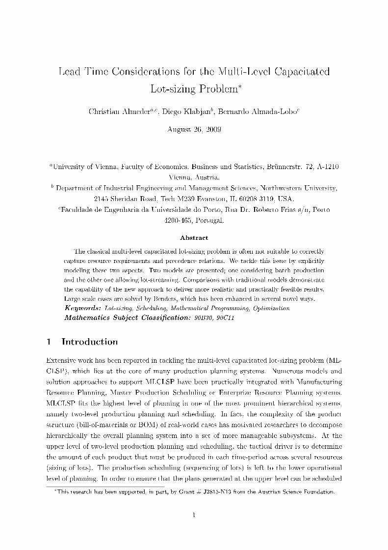
Let us assume a simple example with four items, three machines, and two periods. Table 1

contains all parameters and Figure 1 depicts the product structure. It is assumed that resource

requirements are measured in time units, each machine has a capacity of 1 meaning it is available

throughout the whole period and setup times are zero.

The optimal solution of the according MLCLSP model without lead time can be easily ob-

tained (see Table 2). The total cost is 22 units consisting of the setup cost of 20 units and the

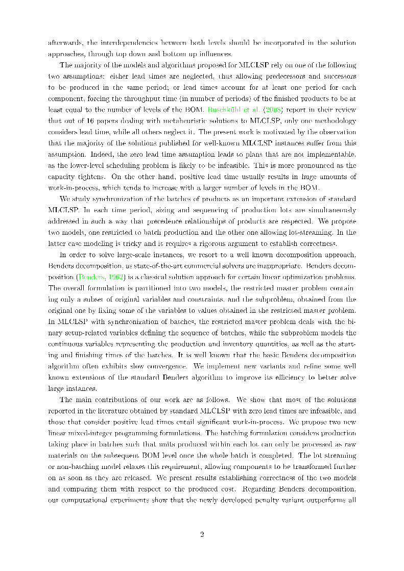
holding cost of 2 units. It is obvious that this solution is not feasible in practice, because before

item 1 can be produced in the �rst period, items 3 and 4 have to be scheduled. Figure 2 shows

two possible implementations of the solution. The �rst one violates the demand requirement, as

5

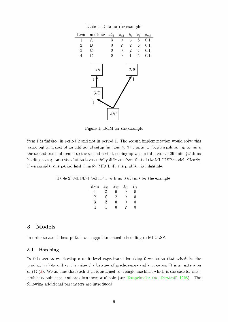
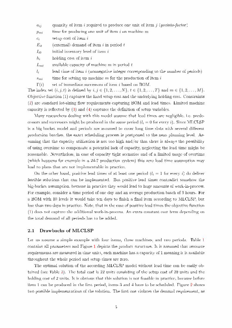
Table 1: Data for the example

item machine di1 di2 hi ci pmi1 A 3 0 3 5 0.12 B 0 2 2 5 0.13 C 0 0 2 5 0.14 C 0 0 1 5 0.1

Figure 1: BOM for the example

item 1 is �nished in period 2 and not in period 1. The second implementation would solve this

issue, but at a cost of an additional setup for item 4. The optimal feasible solution is to move

the second batch of item 4 to the second period, ending up with a total cost of 25 units (with no

holding costs), but this solution is essentially di�erent from that of the MLCLSP model. Clearly,

if we consider one period lead time for MLCLSP, the problem is infeasible.

Table 2: MLCLSP�solution with no lead time for the example

item xi1 xi2 Ii1 Ii21 3 0 0 02 0 2 0 03 3 0 0 04 5 0 2 0

3 Models

In order to avoid these pitfalls we suggest to embed scheduling to MLCLSP.

3.1 Batching

In this section we develop a multi-level capacitated lot-sizing formulation that schedules the

production lots and synchronizes the batches of predecessors and successors. It is an extension

of (1)-(5). We assume that each item is assigned to a single machine, which is the case for most

problems published and test instances available (see Tempelmeier and Derstro�, 1996). The

following additional parameters are introduced:

6

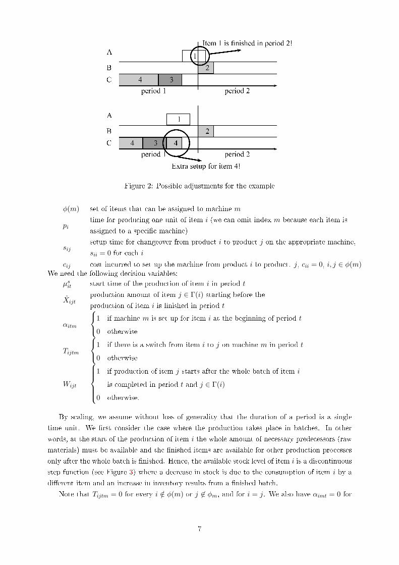
Figure 2: Possible adjustments for the example

φ(m) set of items that can be assigned to machine m

pitime for producing one unit of item i (we can omit index m because each item is

assigned to a speci�c machine)

sijsetup time for changeover from product i to product j on the appropriate machine,

sii = 0 for each i

cij cost incurred to set up the machine from product i to product. j, cii = 0, i, j ∈ φ(m)We need the following decision variables:

µsit start time of the production of item i in period t

X̂ijtproduction amount of item j ∈ Γ(i) starting before theproduction of item i is �nished in period t

αitm

1 if machine m is set up for item i at the beginning of period t

0 otherwise

Tijtm

1 if there is a switch from item i to j on machine m in period t

0 otherwise

Wijt

1 if production of item j starts after the whole batch of item i

is completed in period t and j ∈ Γ(i)

0 otherwise.

By scaling, we assume without loss of generality that the duration of a period is a single

time unit. We �rst consider the case where the production takes place in batches. In other

words, at the start of the production of item i the whole amount of necessary predecessors (raw

materials) must be available and the �nished items are available for other production processes

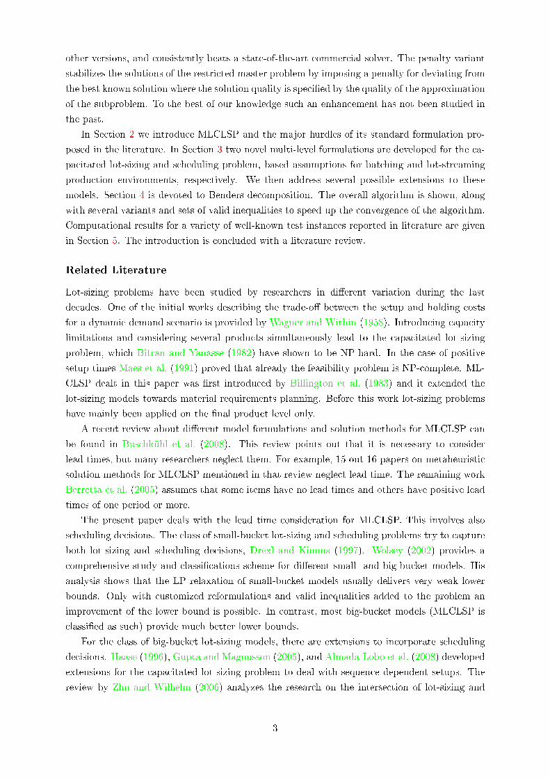
only after the whole batch is �nished. Hence, the available stock level of item i is a discontinuous

step function (see Figure 3) where a decrease in stock is due to the consumption of item i by a

di�erent item and an increase in inventory results from a �nished batch.

Note that Tijtm = 0 for every i /∈ φ(m) or j 6∈ φm, and for i = j. We also have αimt = 0 for

7

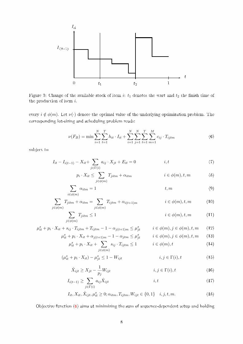
Figure 3: Change of the available stock of item i: t1 denotes the start and t2 the �nish time ofthe production of item i.

every i /∈ φ(m). Let ν(·) denote the optimal value of the underlying optimization problem. The

corresponding lot-sizing and scheduling problem reads:

ν(FB) = minN∑i=1

T∑t=1

hit · Iit +N∑i=1

N∑j=1

T∑t=1

M∑m=1

cij · Tijtm (6)

subject to

Iit − Ii(t−1) −Xit+∑j∈Γ(i)

aij ·Xjt + Eit = 0 i, t (7)

pi ·Xit ≤∑

j∈φ(m)

Tjitm + αitm i ∈ φ(m), t,m (8)

∑i∈φ(m)

αitm = 1 t,m (9)

∑j∈φ(m)

Tjitm + αitm =∑

j∈φ(m)

Tijtm + αi(t+1)m i ∈ φ(m), t,m (10)

∑j∈φ(m)

Tjitm ≤ 1 i ∈ φ(m), t,m (11)

µsit + pi ·Xit + sij · Tijtm + Tijtm − 1− αj(t+1)m ≤ µsjt i ∈ φ(m), j ∈ φ(m), t,m (12)

µsit + pi ·Xit + αj(t+1)m − 1− αjtm ≤ µsjt i ∈ φ(m), j ∈ φ(m), t,m (13)

µsit + pi ·Xit +∑

j∈φ(m)

sij · Tijtm ≤ 1 i ∈ φ(m), t (14)

(µsit + pi ·Xit)− µsjt ≤ 1−Wijt i, j ∈ Γ(i), t (15)

X̂ijt ≥ Xjt −1pjWijt i, j ∈ Γ(i), t (16)

Ii(t−1) ≥∑j∈Γ(i)

aijX̂ijt i, t (17)

Iit, Xit, X̂ijt, µsit ≥ 0;αitm, Tijtm,Wijt ∈ {0, 1} i, j, t,m. (18)

Objective function (6) aims at minimizing the sum of sequence-dependent setup and holding

8

costs. Constraints (7) represent the inventory balances for both components and end-items.

Constraints (8) guarantee that a product is produced only if the machine is set up for it. Note

that we assume that the length of one period is one time unit and capacities are measured in

time units. Therefore, in contrast to constraints (4), we can omit parameter G in this case.

Each machine has to be set up for exactly one product at the beginning of each period from (9).

Constraints (10) carry the setup con�guration state of the machines into the next period and

constraints (11) avoid that there is more than one setup for each item. Disconnected subtours

are removed from any feasible solution by (12). It is easy to see that such constraints also cut

o� subtours that appear in the middle of the sequence (see e.g. Almada-Lobo et al., 2007 or

Almada-Lobo et al., 2008 for details). These constraints also link the starting and �nishing times

of two batches produced one immediately after another. We do not impose the starting times of

the �rst batch in any period to be zero, as there might be some idle time before production starts

(as well as afterwards). Requirements (12) do not de�ne the starting time of the last product to

be produced on each machine, as they are non-active for such cases. We assume that for a cycle

of size greater than one involving item j (αjtm = αj(t+1)m = 1), there occurs only one batch of j

in the �rst position of the production sequence. In case of a path, requirements (13) determine

the starting time of the last product of the sequence. Clearly, (13) are redundant for a cycle.

Inequalities (12)�(14) ensure that the machines are used no longer than their available capacity.

Constraints (15) ensure the coherency between variables Wijt and the start and �nish times of

the batches of predecessors and successors. Note that µsit+pi ·Xit computes the production �nish

time of product i in period t. In case item j starts production before the batch of its predecessor

i is completed in the same period (or in case there is not such batch), i.e. Wijt = 0, constraints(16) and (17) force the quantity of item i required to produce j to be supplied solely from the

initial stock in that period. If Wijt = 1, then (16) and (17) are non-active, and (7) allow the

gross requirements of item i to produce j to be matched from stock and from production in the

same period.

We remark that the way depended batches are synchronized is motivated by Almeder and

Almada-Lobo (2009) where the usage of a secondary resource is synchronized across parallel

machines.

Next we show that formulation FB really models the problem correctly. Let Q be the set of

solutions satisfying constraints (7)�(15) and (18). Set Q admits solutions that have nonnegative

inventory stock for every product at the end of every period (imposed by (7)), but potentially

negative in-period stock. We show that constraints (16) and (17) avoid this case. Now consider

subsets S(i) of items in a given time period t de�ned as

S(i) = {j ∈ Γ(i) : µsjt ≤ µsit + pi ·Xit}.

The following lemma states that there are no negative in-period stocks (note that due to the

batching assumption the condition∑

j∈S(i) aij · Xjt > Ii(t−1) is equivalent to the statement of

having negative in-period stock).

Lemma 1. If x? ∈ Q and x? ful�lls (16) and (17), then∑

j∈S(i) aij ·Xjt ≤ Ii(t−1).

Proof. Let x? ∈ Q. We �rst observe that if j ∈ S(i), then µsjt ≤ µsit + pi ·Xit, which in turn from

9

(15) implies Wijt = 0. Thus if j ∈ S(i), from (16) we obtain X̂ijt ≥ Xjt.

On the other hand, if j ∈ Γ(i)\S(i), then clearly X̂ijt ≥ 0. Combining these two factors we

derive

Ii(t−1) ≥∑j∈Γ(i)

aij · X̂ijt ≥∑j∈S(i)

aij · X̂ijt +∑

j∈Γ(i)\S(i)

aij · X̂ijt ≥∑j∈S(i)

aij · X̂ijt ≥∑j∈S(i)

aij ·Xjt.

This establishes the lemma.

In addition to showing that solutions have no negative in-period stock, we need to assert that

no solutions to the problem are left out.

Lemma 2. Any x? ∈ Q satisfying∑

j∈S(i) aij ·Xjt ≤ Ii(t−1) for every i and t (x∗ has nonnegative

in-period inventory) ful�lls constraints (16) and (17).

Proof. We show this by contradiction. We �rst note that in (16) and (17) we have the freedom

of selecting X̂. As a result we can assume that we have an underlying X̂ijt satisfying (16) but

not (17) for at least one item i′ in a period t′ since otherwise we can always increase X̂ijt to

satisfy (16), but possibly violating (17) even more. Thus we have

X̂i′jt′ ≥ Xjt′ −1pjWi′jt′ j ∈ Γ(i′)

Ii′(t′−1) <∑

j∈Γ(i′)

ai′jX̂i′jt′

Among all such X̂i′jt′ , we pick the smallest one, which we denote by X̂mini′jt′ . By choice we

clearly have

Ii′(t′−1) <∑

j∈Γ(i′)

ai′jX̂mini′jt′ . (19)

According to the de�nition of S(i), the minimal values satisfying (16) are de�ned by

X̂mini′jt′ =

Xjt′ j ∈ S(i′)

0 j ∈ Γ(i′)\S(i′).

Inequality (19) yields

Ii′(t′−1) <∑

j∈Γ(i′)

ai′jX̂mini′jt′ =

∑j∈S(i′)

ai′jX̂mini′jt′ +

∑j∈Γ(i′)\S(i′)

ai′jX̂mini′jt′ =

∑j∈S(i′)

ai′jXjt′ .

This constraint indicates that there is negative in-period inventory and it contradicts our as-

sumption that∑ai′j ·Xjt ≤ Ii′(t′−1).

3.2 Lot-streaming Production (Non-batching)

In the previous model we assumed that components can only be used for the production of

successors if the production batch is completely �nished. If we relax this assumption, we allow to

10

use some already �nished parts of the current production batch for the production of successors.

For this case we assume the idealized situation that there are no transportation times between

di�erent production stages and that inventory levels increase and decrease continuously due to

production and consumption of an item. In principle we have to ensure that during the whole

period the inventory level is nonnegative. Instead of constraints (16) and (17) it is necessary to

replace them with

Ii(t−1) + min(Xit,

1pi

(τ − µsit)+

)≥

∑j∈Γ(i)

aij min(Xjt,

1pj

(τ − µsjt

)+)i, t, τ ∈ [0, 1], (20)

where x+ := max(x, 0).This set of constraints ensures that, for every time point τ in period t, the initial inventory

plus the production of item i until τ is not less than the consumption of item i due to the

production of successors. Note that the external demand Eit only occurs at the end of the

period. Unfortunately there is an in�nite number of such constraints. The next result asserts

that only a �nite number of τ values su�ces.

Theorem 3. It is su�cient and necessary to ful�ll constraints (7) and (20) at the beginning of

the production of item i (τ = µsit) and at the end of the production of each successor k ∈ Γ(i)(τ = µskt+pkXkt) in order to maintain a nonnegative inventory level throughout the whole period

t.

Proof. We �x item i. Let us �rst consider the case when there is no production of item i in

period t (Xit = 0). If there is no production, the in-period inventory level of item i is non-

increasing throughout the period. Hence it reaches the minimum at the end of the period. Since

constraints (7) ensure that there is a nonnegative stock level at the end of each period, the

in-period inventory level can never be negative. To show the other way around, because of (7),

the following derivation shows that (20) is ful�lled for all τ :

Ii(t−1) + min(Xit,

1pi

(τ − µsit)+

)= Ii(t−1) = Iit −Xit + Eit +

∑j∈Γ(i)

aijXjt ≥

≥∑j∈Γ(i)

aijXjt ≥∑j∈Γ(i)

aij min(Xjt,

1pj

(τ − µsjt

)+).

Now let us consider the case of a production of item i in period t (Xit > 0). We divide the

period into three parts. Let t1 de�ne the start of the production of item i (t1 = µsit), and t2 the

end of the production of item i (t2 = µsit + piXit). Furthermore, note that1pi

is the production

rate of item i,aij

pjis the consumption rate of item i due to the production of successor j, and

the in-period inventory level Iit(τ) is a piecewise linear function of τ .

Let �rst τ ∈ [0, t1]. During this period only consumption of item i might occur (Iit(τ) is non-increasing), so it is su�cient and necessary that at time t1 the inventory level is nonnegative,

which is equivalent to constraints (20) at τ = t1 = µsit.

Consider now τ ∈ [t2, 1]. After t2 again only consumption might occur and the in-period

inventory level is non-increasing (Iit(τ) is again non-increasing). For the the time span from t2

11

to the end of the period it is su�cient and necessary to have nonnegative inventory at the end

of the period. This is assured by constraints (7).

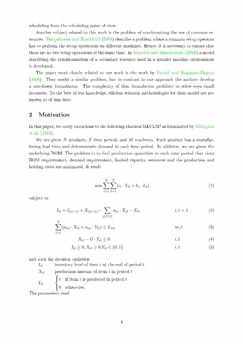
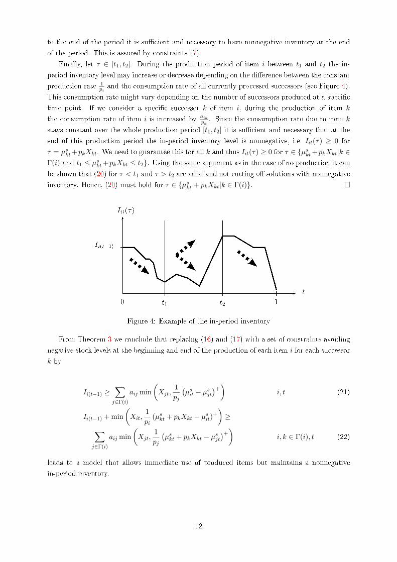
Finally, let τ ∈ [t1, t2]. During the production period of item i between t1 and t2 the in-

period inventory level may increase or decrease depending on the di�erence between the constant

production rate 1piand the consumption rate of all currently processed successors (see Figure 4).

This consumption rate might vary depending on the number of successors produced at a speci�c

time point. If we consider a speci�c successor k of item i, during the production of item k

the consumption rate of item i is increased by aikpk. Since the consumption rate due to item k

stays constant over the whole production period [t1, t2] it is su�cient and necessary that at the

end of this production period the in-period inventory level is nonnegative, i.e. Iit(τ) ≥ 0 for

τ = µskt+pkXkt. We need to guarantee this for all k and thus Iit(τ) ≥ 0 for τ ∈ {µskt+pkXkt|k ∈Γ(i) and t1 ≤ µskt+pkXkt ≤ t2}. Using the same argument as in the case of no production it canbe shown that (20) for τ < t1 and τ > t2 are valid and not cutting o� solutions with nonnegative

inventory. Hence, (20) must hold for τ ∈ {µskt + pkXkt|k ∈ Γ(i)}.

Figure 4: Example of the in-period inventory

From Theorem 3 we conclude that replacing (16) and (17) with a set of constraints avoiding

negative stock levels at the beginning and end of the production of each item i for each successor

k by

Ii(t−1) ≥∑j∈Γ(i)

aij min(Xjt,

1pj

(µsit − µsjt

)+)i, t (21)

Ii(t−1) + min(Xit,

1pi

(µskt + pkXkt − µsit)+

)≥∑

j∈Γ(i)

aij min(Xjt,

1pj

(µskt + pkXkt − µsjt

)+)i, k ∈ Γ(i), t (22)

leads to a model that allows immediate use of produced items but maintains a nonnegative

in-period inventory.

12

Hence, the model for the non-batching case reads:

ν(FNB) = minN∑i=1

T∑t=1

hit · Iit +N∑i=1

N∑j=1

T∑t=1

M∑m=1

cij · Tijtm

subject to (7)− (15), (21), (22)

Iit, Xit, µsit ≥ 0;αitm, Tijtm,Wijt ∈ {0, 1} i, j, t,m

This is a nonlinear model that can be linearized. We show the underlying linearization of

(21) and (22) in Appendix A.

We prove in the following theorem that FB is a special case of FNB and, as such, the optimal

value of FNB is at least as good as FB's.

Theorem 4. We have v(FB) ≥ v(FNB).

Proof. We demonstrate the statement by showing that adding constraints (16) and (17) to FNB

constraints (21) and (22) become redundant and can be dropped.

Consider S(i) = {j ∈ Γ(i) : µsit ≥ µsjt}. Constraints (21) are then equivalent to Ii(t−1) ≥∑j∈S(i) aij min

(Xjt,

1pj

(µsit − µsjt

)). If j ∈ S(i), then (15) imposes Wijt = 0 and X̂ijt ≥ Xjt.

Using (16) and (17), we obtain

Ii(t−1) ≥∑j∈Γ(i)

aijX̂ijt ≥∑j∈S(i)

aij ·Xjt ≥∑j∈S(i)

aij min(Xjt,

1pj

(µsit − µsjt

))i, t,

making constraint (21) redundant.

Let Q(i, k), k ∈ Γ(i) denote Q(i, k) = {j : j ∈ Γ(i) and µskt + pkXkt ≥ µsjt}. The right

hand-side of (22) can then be simpli�ed to

∑j∈Q(i,k)

aij min(Xjt,

1pj

(µskt + pkXkt − µsjt

)).

Let us now distinguish two cases: µskt + pkXkt ≤ µsit or µskt + pkXkt > µsit.

We start by µskt+pkXkt ≤ µsit. Since µskt ≤ µsit+pi ·Xit, from (15) clearlyWikt = 0. Moreover,

Wijt = 0 for every j in Q(i, k), which implies X̂ijt ≥ Xjt. Thus,

Ii(t−1) ≥∑

j∈Q(i,k)

aij ·Xjt ≥∑

j∈Q(i,k)

aij min(Xjt,

1pj

(µskt + pkXkt − µsjt

))i, k ∈ Γ(i), t.

Let now µskt + pkXkt > µsit. We have to further consider two di�erent scenarios.

If µskt + pkXkt < µsit + piXit, then similarly to the above case, it follows that Wikt = 0 and

13

Wijk = 0 for every j in Q(i, k). In terms it yields

Ii(t−1) + min(Xit,

1pi

(µskt + pkXkt − µsit))≥ Ii(t−1) ≥

≥∑

j∈Q(i,k)

aij ·Xjt ≥∑

j∈Q(i,k)

aij min(Xjt,

1pj

(µskt + pkXkt − µsjt

)),

making (22) redundant.

Finally let µskt + pkXkt ≥ µsit + piXit. In this case (22) reads

Ii(t−1) + min(Xit,

1pi

(µskt + pkXkt − µsit))

= Ii(t−1) +Xit ≥

≥∑

j∈Q(i,k)

aij min(Xjt,

1pj

(µskt + pkXkt − µsjt

)).

It is easy to see that this condition is dominated by Ii(t−1) + Xit ≥∑

j∈Γ(i) aij · Xjt, which is

derived from (7) given that Iit and Eit are non-negative.

3.3 Extensions

An interesting extension is a combination of the batching and lot-streaming cases, i.e. the raw

materials might be delivered continuously to the production process of item i, but the newly

produced items are only available if the whole batch is �nished. In such a case we have to ensure

that the whole production of successors can be supplied from stock of item i until the production

is �nished. In order to achieve this we replace (22) by

Ii(t−1) ≥∑j∈Γ(i)

aij min(Xjt, pj

(µsit + piXit − µsjt

)+)i, t. (23)

In (23) we have replaced the start time µsit of the production of item i by the �nish time

µsit + piXit.

The proposed models could be extended in several di�erent directions in order to adapt them

to other production scenarios. The option of using overtime to compensate for a lack of capacities

is easily introduced by relaxing constraints (14). Furthermore, in constraints (8), (12), (13), and

(16) a large number M must be introduced and the objective function must be extended by a

penalty term for the use of overtime.

The synchronization model could also be extended for a parallel machine scenario where

each item might be produced on several di�erent machines. For that purpose it is necessary to

di�erenciate the production amounts Xit and the starting times µsit for the the di�erent machines

m, as well as the synchronization variables would have to be extended to Wijtmm′ and X̂ijtmm′ .

Both versions, the batching and lot-streaming cases, represent extreme situations, especially

the continuous production case where it is possible to produce subsequent items in the BOM at

the same time. If we want to model a situation where it is not necessary to wait for the whole

batch to be �nished before items can be retrieved and used for further production steps, we

might introduce a minimum production lead time τi and substitute in constraints (21) and (22)

14

the starting time of item i with the term µsit + τi.

4 Benders Decomposition

Large-scale instances of the proposed models cannot be e�ciently solved by commercial IP

solvers. For this reason we resort to decomposition approaches, namely Benders decomposition,

Benders (1962). We focus on the batching case, but all other cases can be treated in a similar

fashion.

To this end, let us introduce the following function, where−→T = (Tijtm)i,j,t,m,

−→W = (Wijt)i,j,t,

−→α = (αitm)i,t,m are given:

f(−→T ,−→W,−→α ) = min

N∑i=1

T∑t=1

hit · Iit (24)

Iit − Ii(t−1) −Xit +∑j∈Γ(i)

aij ·Xjt = −Eit i, t (25)

pi ·Xit ≤∑

j∈φ(m)

Tjitm + αitm i ∈ φ(m), t,m (26)

µsit − µsjt + pi ·Xit ≤ −sij · Tijtm − Tijtm + 1 + αj(t+1)m (i, j) ∈ φ(m), t,m(27)

µsit + pi ·Xit − µsjt ≤ −αj(t+1)m + 1 + αjtm (i, j) ∈ φ(m), t,m(28)

µsit + pi ·Xit ≤ 1−∑

j∈φ(m)

sij · Tijtm i ∈ φ(m), t (29)

µsit − µsjt + pi ·Xit ≤ 1−Wijt i, j ∈ Γ(i), t (30)

Xjt − X̂ijt ≤1pjWijt i, j ∈ Γ(i), t (31)∑

j∈Γ(i)

aijX̂ijt − Ii(t−1) ≤ 0 i, t (32)

I,X, X̂, µ ≥ 0. (33)

We note that evaluation of f corresponds to solving an LP. Then our batching model can be

rewritten as

ν(FB) = minN∑i=1

N∑j=1

T∑t=1

M∑m=1

cij · Tijtm + f(−→T ,−→W,−→α ) (34)

∑i∈φ(m)

αitm = 1 t,m (35)

∑j∈φ(m)

Tjitm + αitm =∑

j∈φ(m)

Tijtm + αi(t+1)m i ∈ φ(m), t,m (36)

∑j∈φ(m)

Tjitm ≤ 1 i ∈ φ(m), t,m (37)

α, T,W binary. (38)

15

We consider the dual polyhedron of the LP de�ning f . To this end, let Π be a dual vector

corresponding to (25)-(32), respectively. For ease of notation we denote by q(−→T ,−→W,−→α ) the

vector of all right-hand sides in the same LP. Let K be the �nite set of all extreme vertices and

J the �nite set of all extreme rays of the dual polyhedron. Then by basic LP theory and the

principles of Benders we have

ν(FB) = minN∑i=1

N∑j=1

T∑t=1

M∑m=1

cij · Tijtm + s (39)

subject to (35)− (37) (40)

q(−→T ,−→W,−→α )Π− s ≥ 0 Π ∈ K (41)

q(−→T ,−→W,−→α )Π ≤ 0 Π ∈ J (42)

−→α ,−→T ,−→W binary. (43)

This reformulation has a lower number of variables, but many more rows. Indeed, the rows need

to be generated dynamically on the �y. Algorithm 1 presents the basic row generation algorithm.

(The exposition in Step 16 exploits the fact that ν(FB) > 0.)

1: Start with K = J = ∅.2: loop

3: Solve (39)-(43) by considering the incumbent K,J .4: if this mixed integer program is infeasible then5: Exit, the original problem is infeasible.6: end if

7: Let−→T ∗,−→W ∗,−→α ∗, s∗ be the resulting optimal solution.

8: Solve the linear program f(−→T ∗,−→W ∗,−→α ∗).

9: if this linear program is feasible then10: Let Π∗ be an optimal dual solution.11: Set K = K ∪ {Π∗}.12: else

13: Let Π∗ be an extreme ray.14: Set J = J ∪ {Π∗}.15: end if

16: if |s∗| > 0 and s∗−f(−→T ∗,−→W ∗,−→α ∗)

|s∗| ≤ some relative tolerance then17: Exit.18: end if

19: end loop

Algorithm 1: The Benders algorithm

The problem (39)-(43) over a subset of K,J is called the restricted master problem (RMP).

The Benders algorithm is known to exhibit slow convergence mostly due to degeneracy of the

underlying LP behind f . We have tried several variants, some of them being new. Next we

describe them one by one.

Convex Combinations This idea originates in Klabjan et al. (2000) in the context of column

generation, but it was later used in a Benders framework by Smith (2004). The key concept

is to consider prior solutions to the RMP and then to modify the evaluation of f to also

optimize over best convex combination multipliers.

16

Let (−→T ∗i,

−→W ∗i,−→α ∗i) for i = 1, . . . , κ be optimal solutions in Step 7 over the last κ iterations

with feasible f , where κ is a parameter. Instead of evaluating f , we evaluate

min f(κ∑i=1

λi−→T ∗i,

κ∑i=1

λi−→W ∗i,

κ∑i=1

λi−→α ∗i) +

κ∑k=1

λk

N∑i=1

N∑j=1

T∑t=1

M∑m=1

cij · T ∗kijtm

0 ≤ λ ≤ 1κ∑i=1

λi = 1 .

It is not di�cult to see that this is an LP with variables λ, I,X, X̂, µ.

After solving this optimization problem in a given iteration, we get the underlying dual

values and add the corresponding cut. This convex combination problem is not solved in

each iteration of Algorithm 1, but every κ iteration, i.e., once it is solved in an iteration,

standard Benders is applied for the next κ iterations, which are then followed by a single

iteration with convex combination.

Duplicate Variables A potential drawback of our reformulation is the fact that binary vari-

ables W are not present in constraints (35)-(37). To remedy this we can replicate these

variables in both the RMP and in evaluating f . To carry out this idea, the RMP remains

intact, but f is modi�ed by consideringW as a continuous variable. The resulting modi�ed

f , denoted by f̄ , becomes only a function of−→T and −→α , i.e., f̄ = f̄(

−→T ,−→α ) and W 's are

continuous variables in f̄ . The dual prices are obtained as before and the underlying cuts

do not change.

It can be shown that the optimal value of such a Benders approach is less than or equal to

ν(FB) and larger than or equal to the optimal value of the LP relaxation of ν(FB).

Deviation Penalties In column generation there are known box-step type approaches to sta-

bilize the underlying dual prices, Briant et al. (2008), du Merle et al. (1999). These

approaches impose a deviation penalty in the subproblem to smoothly guide or stabilize

the dual prices.

In Benders, the dual prices from the subproblem do not require stabilization (even though

there are other issues with the dual prices such as degeneracy and dominance), however

the solutions to RMP tend to bounce around. It thus seems plausible to speed up the

algorithm by stabilizing the RMP solutions. To this end, let−→T ′,−→W ′,−→α ′ be a past solution

of RMP and R a penalty. We modify the objective function of RMP to

N∑i=1

N∑j=1

T∑t=1

M∑m=1

cij · Tijtm + s+R‖(−→T ,−→W,−→α )− (

−→T ′,−→W ′,−→α ′)‖ .

The challenge now becomes how to update R, which is initially set to a very large number,

and−→T ′,−→W ′,−→α ′. For the latter, we keep track of the minimum h = s∗−f(

−→T ∗,−→W ∗,−→α ∗)

|s∗| observed

so far. Let us denote this value by hmin. In a given iteration, if h < hmin, we reset hmin = h

and update (−→T ′,−→W ′,−→α ′) = (

−→T ∗,−→W ∗,−→α ∗). If hmin is below the accepted tolerance level,

17

then we decrease R, e.g., R = R/2. If R becomes too small, we remove the penalty term

altogether.

A known technique for generating Pareto non-dominant cuts is presented in Magnanti and

Wong (1981). We did not evaluate it since, �rst, it is hard to �nd a core point, which is required

in their approach, and second, our past experience has shown no bene�ts by using the suggested

core approach.

To further strengthen the RMP, we add the following valid inequalities.

Vjt ≥ Vit +QmTijmt − (Qm − 1)−Qmαimt m, i ∈ φ(m), j, t (44)

Wijt ≤ αimt +∑

k∈φ(m)

Tkimt m, i ∈ φ(m), j, t

Wijt ≤ αjmt +∑

k∈φ(m)

Tkjmt m, i ∈ φ(m), j, t

Here Qm is the total number of items that can be assigned to machinem and Vit are new auxiliary

variables. The full derivation of these inequalities can be found in Almada-Lobo et al. (2007)

with appropriate adjustments. Valid inequalities (44) follow from the fact that T variables either

form a path or cycle in an appropriately de�ned network with α controlling if it is a path or

cycle.

5 Computational Experiments

All computational experiments were coded in C++ using CPLEX 11.1 and Concert 2.6 on an

Intel Pentium D with 3.2 GHz CPU and 4 GB of random access memory. In Section 5.1 we

focus on the IP formulations FB and FNB and their comparison with MLCLSP. Secion 5.2 is

dedicated to Benders.

5.1 Comparing with MLCLSP

All models in this section are solved by CPLEX. Furthermore, we used the well-known (l, S)valid inequalities adapted by Clark and Armentano (1995) for the multi-level case. We add them

dynamically within the branch-and-cut framework of CPLEX.

5.1.1 MLCLSP with Zero Lead Time and no Setup Carryover

Considering that the proposed model incorporates more details than MLCLSP, we �rst evaluate

if solutions derived from the traditional MLCLSP model would also be optimal or feasible for

our approach. For this purpose we considered 4 classes of instances proposed by Tempelmeier

and Derstro� (1996). Classes A and B are small instances with 10 items produced on 3 machines

and a planning horizon of 4 periods. Class A instances consider setup cost but no setup times,

whereas class B instances include also setup times. These classes are small enough that MLCLSP

with zero lead time and no setup carryover can be solved easily with CPLEX within a second.

Classes C and D are larger instances (40 items, 6 machines, 16 periods). For most of these

instances optimal solutions of MLCLSP are unknown. We take the best known solutions for

18

these classes obtained by a heuristic method proposed in Almeder (2009). All classes contain

instances with a general and assembly product structure, with di�erent demand pro�les and

di�erent levels of capacity utilization.

The classical MLCLSP does not consider setup carryover. To avoid setup carryover in our

formulation we introduce additional items (one for each machine) with no demand and force

that setup carryovers are only possible for those additional items. The setup times and costs

into these items are set to zero. The production quantities obtained by solving the MLCLSP

are �xed in our formulation (6)-(18) such that we only determine the production sequences and

start and �nish times. We let CPLEX run for at most ten minutes and classify the outcomes in

three di�erent categories:

Infeasible: CPLEX reports that the problem is infeasible, i.e. it is not possible to �nd a capacity

feasible solution with the given production amount respecting synchronization conditions,

Feasible: CPLEX is able to �nd a capacity feasible solution with the given production quanti-

ties, which considers synchronization,

Unknown: CPLEX is neither able to generate a feasible solution, nor to prove infeasibility.

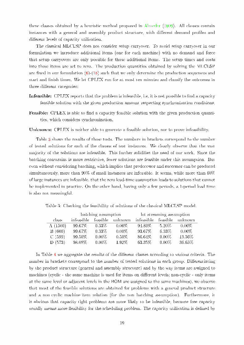
Table 3 shows the results of these tests. The numbers in brackets correspond to the number

of tested solutions for each of the classes of test instances. We clearly observe that the vast

majority of the solutions are infeasible. This further solidi�es the need of our work. Since the

batching constraint is more restrictive, fewer solutions are feasible under this assumption. But

even without considering batching, which implies that predecessor and successor can be produced

simultaneously, more than 90% of small instances are infeasible. It seems, while more than 60%

of large instances are infeasible, that the zero lead-time assumption leads to solutions that cannot

be implemented in practice. On the other hand, having only a few periods, a 1-period lead time

is also not meaningful.

Table 3: Checking the feasibility of solutions of the classical MLCLSP model.

batching assumption lot-streaming assumptionclass infeasible feasible unknown infeasible feasible unknown

A (1500) 99.67% 0.33% 0.00% 94.80% 5.20% 0.00%B (600) 99.67% 0.33% 0.00% 93.67% 6.33% 0.00%C (599) 99.50% 0.00% 0.50% 86.64% 0.00% 13.36%D (573) 98.08% 0.00% 1.92% 63.35% 0.00% 36.65%

In Table 4 we aggregate the results of the di�erent classes according to various criteria. The

number in brackets correspond to the number of tested solutions in each group. Di�erentiating

by the product structure (general and assembly structure) and by the way items are assigned to

machines (cyclic - the same machine is used for items on di�erent levels; non-cyclic - only items

at the same level or adjacent levels in the BOM are assigned to the same machines), we observe

that most of the feasible solutions are obtained for problems with a general product structure

and a non-cyclic machine-item relation (for the non batching assumption). Furthermore, it

is obvious that capacity-tight problems are more likely to be infeasible, because free capacity

usually means more �exibility for the scheduling problem. The capacity utilization is de�ned by

19

the total capacity requirement for production and setup for each machine divided by the total

available capacity of that machine. Also, the setup cost level has an impact on the feasibility

of the solution. High setup costs tend to generate solutions with large batches which are more

di�cult to schedule than smaller batches.

Table 4: Breakdown with respect to BOM structure, capacity utilization, and setup cost.

batching assumption lot-streaming assumptiongroup infeasible feasible unknown infeasible feasible unknown

general-noncyclic (823) 99.51% 0.00% 0.49% 73.27% 12.76% 13.97%general-cyclic (814) 99.02% 0.86% 0.12% 94.35% 1.35% 4.30%

assembly-noncyclic (811) 99.38% 0.00% 0.62% 91.86% 0.00% 8.14%assembly-cyclic (824) 99.51% 0.00% 0.49% 91.02% 0.00% 8.98%

capacity util. 90% (641) 100.00% 0.00% 0.00% 97.97% 0.00% 2.03%capacity util. 70% (657) 100.00% 0.00% 0.00% 87.67% 3.04% 9.28%capacity util. 50% (660) 97.42% 1.06% 1.52% 80.45% 5.91% 13.64%

setup cost - low (653) 96.78% 1.07% 2.14% 81.62% 5.97% 12.40%setup cost - med. (656) 100.00% 0.00% 0.00% 88.41% 3.51% 8.08%setup cost - high (656) 100.00% 0.00% 0.00% 91.62% 2.13% 6.25%

5.1.2 MLCLSP with Zero Lead Time and Setup Carryover

In addition to the classical MLCLSP the proposed model considers setup carryover. We have

applied the full model with synchronization to the test classes A and B in order to gain some

insights about the computational behavior of the model. The results are compared to the solution

of the classical MLCLSP with setup carryover. The solution of that model is a lower bound for

the solution of model (6)-(18).

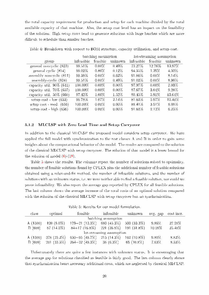
Table 5 shows the results. The columns report the number of solutions solved to optimality,

the number of feasible solutions found by CPLEX plus the additional number of feasible solutions

obtained using a relax-and-�x method, the number of infeasible solutions, and the number of

solutions with an unknown status, i.e. we were neither able to �nd a feasible solution, nor could we

prove infeasibility. We also report the average gap reported by CPLEX for all feasible solutions.

The last column shows the average increase of the total costs of an optimal solution compared

with the solution of the classical MLCLSP with setup carryover but no synchronization.

Table 5: Results for our model formulation.

class optimal feasible infeasible unknown avg. gap cost incr.

batching assumptionA (1500) 120 (8.0%) 179+21 (13.3%) 680 (45.3%) 500 (33.3%) 9.86% 27.20%B (600) 87 (14.5%) 84+17 (16.8%) 221 (36.8%) 191 (31.8%) 10.26% 25.40%

lot-streaming assumptionA (1500) 378 (25.2%) 650+95 (49.7%) 215 (14.3%) 162 (10.8%) 9.80% 8.82%B (600) 201 (33.5%) 264+32 (49.3%) 38 (6.3%) 65 (10.8%) 7.63% 8.53%

Unfortunately there are quite a few instances with unknown status. It is encouraging that

the average gap for solutions classi�ed as feasible is fairly good. The last column clearly shows

that synchronization bears necessary additional costs, which are neglected by classical MLCLSP.

20

5.1.3 MLCLSP with One Period Lead Time and Setup Carryover

One way to overcome the feasibility problem of the MLCLSP is to consider a minimum lead time

of one period. As aforementioned this lead time may cause a substantial increase of inventory.

Tempelmeier and Buschkühl (2009) used an extension of the class B test instances for MLCLSP

with lead time and setup carryover. In order to guarantee feasibility they added two additional

periods at the beginning with no external demand (in total now 6 periods). Since the problems

have a three level product structure it is possible to satisfy an end-item demand after the third

period. We will denote the new class of instances as B6.

We solve the test instances using the classical MLCLSP without synchronization, but with

one period lead time (as for example described by Tempelmeier and Buschkühl, 2009), as well

as using our new model formulation with synchronization. Since the model with synchronization

is much harder to solve, we apply a 10 minute run time limit to CPLEX. Table 6 compares the

new solutions obtained by using the synchronization feature. The columns show the number of

solutions solved to optimality, the number of feasible solutions, the number of instances where no

solution has been obtained, the number of improved solutions and the average cost improvement

(improvement of the upper bound) of the synchronization model compared with the MLCLSP

with lead time.

For the batching case we can solve 114 instances to optimality, for 483 instances we �nd a

feasible solution and only for 3 instances we are not able to compute a feasible solution within

the speci�ed run time. All those three instances have an assembly product structure, cyclic

machine-item relations and a high capacity utilization. For the non-batching case we are able

to solve more instances to optimality. For the non-batching case 140 instances can be solved to

optimality and for all other instances we obtain feasible solutions.

The column labeled UB impr. denotes the average improvement of the objective function of

the best solution found (optimal or feasible) compared to the optimal solution of the MLCLSP

with lead time. Considering lead time in a big-bucket model leads to a clear overestimate of the

optimal costs of at least 27.5% for batching and 37.6% for lot-streaming due to the increased

inventory levels carried from one-period to the next one just to maintain feasibility of the solution.

5.2 Benders Algorithms

In this section we compare the enhancement strategies of the Benders algorithm. In addition,

we compare Benders with CPLEX. All of the experiments were carried out on large instances

of class D (same as those used before) and class 6 proposed by Tempelmeier and Buschkühl

(2009) with a time limit of one hour for both Benders and CPLEX. Class 6 instances are of the

same size and similar structure as class D instances. The di�erence is that class 6 instances were

designed to be feasible for MLCLSP with lead time and setup carryover. Thus, they are also

feasible for our model formulation. Class D instances were designed for the MLCLSP without

lead time. Hence, some of them might be infeasible and backlogging is necessary. In order to

avoid technical and development di�culties with a possibly infeasible f , we allow backlogging

(see (25)), but we heavily penalize it.

Tables 7 and 8 summarize the most important �ndings. All of the values in both tables

present the relative di�erence with respect to the objective value of the solution obtained by

21

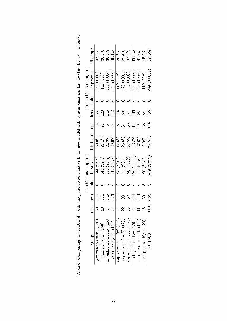
Table6:

Com

paringtheMLCLSPwithoneperiodlead

timewiththenew

modelwithsynchronizationfortheclassB6testinstances.

batchingassumption

nobatchingassumption

group

opt.

feas.

unk.

improved

UBimpr.

opt.

feas.

unk.

improved

UBimpr.

general-noncyclic(150)

39111

0144(96%

)30.0%

8466

0150(100%)

43.8%

general-cyclic(150)

49101

0146(97%

)27.1%

21129

0149(99%

)30.1%

assembly-noncyclic(150)

2145

3110(73%

)21.3%

5145

0150(100%)

36.1%

assembly-cyclic(150)

24126

0149(99%

)30.0%

38112

0150(100%)

40.4%

capacityutil.60%

(120)

0117

395

(79%

)17.6%

6114

0119(99%

)30.6%

capacityutil47%

(120)

2298

0111(93%

)26.6%

3189

0120(100%)

38.4%

capacityutil.33%

(120)

5862

0120(100%)

37.5%

6654

0120(100%)

43.6%

setupcost-low(120)

6114

0120(100%)

48.2%

14106

0120(100%)

66.6%

setupcost-med.(120)

11109

0119(99%

)27.6%

2595

0120(100%)

41.3%

setupcost-high(120)

4869

390

(75%

)9.9%

5664

0119(99%

)15.0%

all(600)

114

483

3549(92%)

27.5%

148

452

0599(100%)

37.6%

22

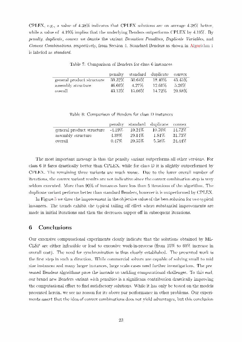
CPLEX, e.g., a value of 4.38% indicates that CPLEX solutions are on average 4.38% better,

while a value of -4.19% implies that the underlying Benders outperforms CPLEX by 4.19%. By

penalty, duplicate, convex we denote the variant Deviation Penalties, Duplicate Variables, and

Convex Combinations, respectively, from Section 4. Standard Benders as shown in Algorithm 1

is labeled as standard.

Table 7: Comparison of Benders for class 6 instances

penalty standard duplicate convex

general product structure -39.32% 30.64% 18.40% 43.45%assembly structure -46.66% 4.27% 12.61% 5.26%overall -43.13% 15.06% 14.72% 20.88%

Table 8: Comparison of Benders for class D instances

penalty standard duplicate convex

general product structure -4.19% 10.24% 10.76% 14.72%assembly structure 4.38% 29.14% 1.81% 31.73%overall 0.47% 20.55% 5.58% 24.44%

The most important message is that the penalty variant outperforms all other versions. For

class 6 it fares drastically better than CPLEX, while for class D it is slightly outperformed by

CPLEX. The remaining three variants are much worse. Due to the lower overall number of

iterations, the convex variant results are not indicative since the convex combination step is very

seldom executed. More than 90% of instances have less than 5 iterations of the algorithm. The

duplicate variant performs better than standard Benders, however it is outperformed by CPLEX.

In Figure 5 we show the improvement in the objective value of the best solution for two typical

instances. The trends exhibit the typical tailing o� e�ect where substantial improvements are

made in initial iterations and then the decreases tapper o� in subsequent iterations.

6 Conclusions

Our extensive computational experiments clearly indicate that the solutions obtained by ML-

CLSP are either infeasible or lead to excessive work-in-process (from 15% to 60% increase in

overall cost). The need for synchronization is thus clearly established. The presented work is

the �rst step in such a direction. While commercial solvers are capable of solving small to mid

size instances and many larger instances, large-scale cases need further investigations. The pre-

sented Benders algorithms pave the inroads to tackling computational challenges. To this end,

our brand new Benders variant with penalties is a signi�cant contribution drastically improving

the computational e�ort to �nd satisfactory solutions. While it has only be tested on the models

presented herein, we see no reason for its above par performance in other problems. Our experi-

ments assert that the idea of convex combinations does not yield advantages, but this conclusion

23

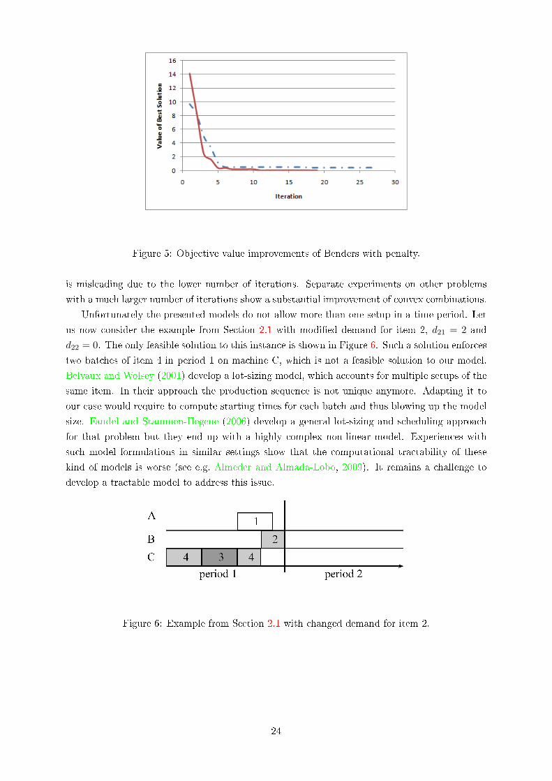
Figure 5: Objective value improvements of Benders with penalty.

is misleading due to the lower number of iterations. Separate experiments on other problems

with a much larger number of iterations show a substantial improvement of convex combinations.

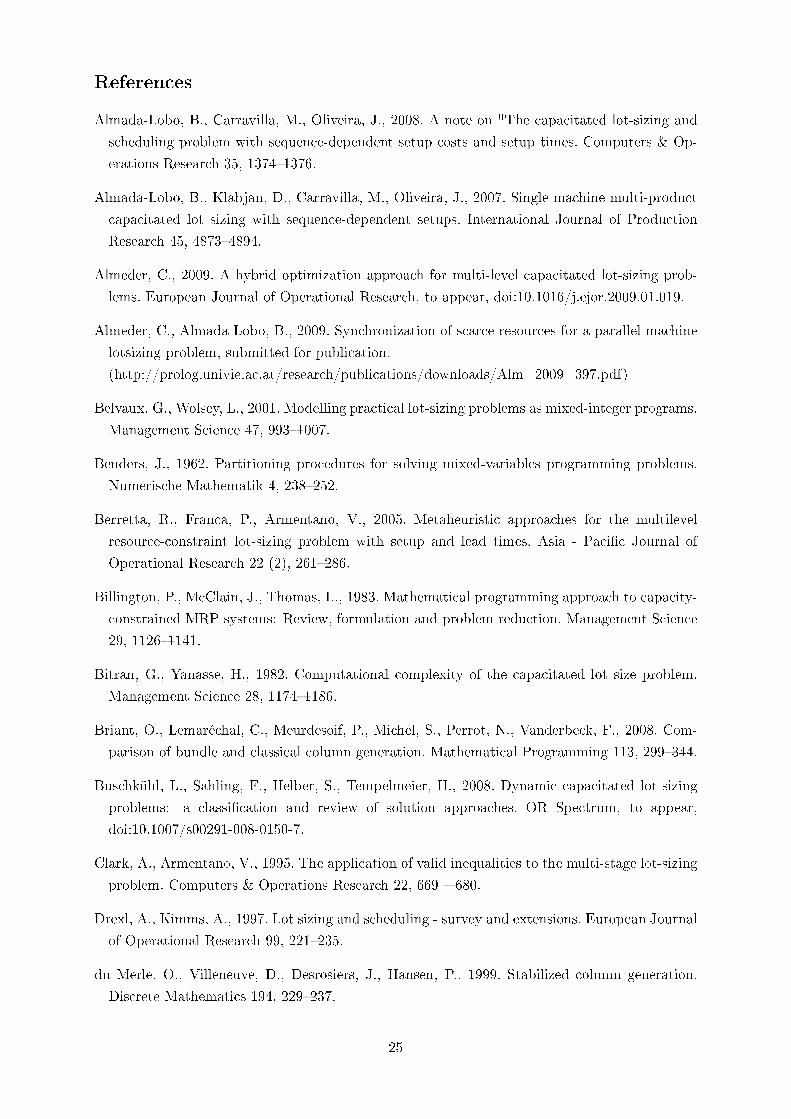
Unfortunately the presented models do not allow more than one setup in a time period. Let

us now consider the example from Section 2.1 with modi�ed demand for item 2, d21 = 2 and

d22 = 0. The only feasible solution to this instance is shown in Figure 6. Such a solution enforcestwo batches of item 4 in period 1 on machine C, which is not a feasible solution to our model.

Belvaux and Wolsey (2001) develop a lot-sizing model, which accounts for multiple setups of the

same item. In their approach the production sequence is not unique anymore. Adapting it to

our case would require to compute starting times for each batch and thus blowing up the model

size. Fandel and Stammen-Hegene (2006) develop a general lot-sizing and scheduling approach

for that problem but they end up with a highly complex non-linear model. Experiences with

such model formulations in similar settings show that the computational tractability of these

kind of models is worse (see e.g. Almeder and Almada-Lobo, 2009). It remains a challenge to

develop a tractable model to address this issue.

Figure 6: Example from Section 2.1 with changed demand for item 2.

24

References

Almada-Lobo, B., Carravilla, M., Oliveira, J., 2008. A note on "The capacitated lot-sizing and

scheduling problem with sequence-dependent setup costs and setup times. Computers & Op-

erations Research 35, 1374�1376.

Almada-Lobo, B., Klabjan, D., Carravilla, M., Oliveira, J., 2007. Single machine multi-product

capacitated lot sizing with sequence-dependent setups. International Journal of Production

Research 45, 4873�4894.

Almeder, C., 2009. A hybrid optimization approach for multi-level capacitated lot-sizing prob-

lems. European Journal of Operational Research, to appear, doi:10.1016/j.ejor.2009.01.019.

Almeder, C., Almada-Lobo, B., 2009. Synchronization of scarce resources for a parallel machine

lotsizing problem, submitted for publication.

(http://prolog.univie.ac.at/research/publications/downloads/Alm_2009_397.pdf)

Belvaux, G., Wolsey, L., 2001. Modelling practical lot-sizing problems as mixed-integer programs.

Management Science 47, 993�1007.

Benders, J., 1962. Partitioning procedures for solving mixed-variables programming problems.

Numerische Mathematik 4, 238�252.

Berretta, R., Franca, P., Armentano, V., 2005. Metaheuristic approaches for the multilevel

resource-constraint lot-sizing problem with setup and lead times. Asia - Paci�c Journal of

Operational Research 22 (2), 261�286.

Billington, P., McClain, J., Thomas, L., 1983. Mathematical programming approach to capacity-

constrained MRP systems: Review, formulation and problem reduction. Management Science

29, 1126�1141.

Bitran, G., Yanasse, H., 1982. Computational complexity of the capacitated lot size problem.

Management Science 28, 1174�1186.

Briant, O., Lemaréchal, C., Meurdesoif, P., Michel, S., Perrot, N., Vanderbeck, F., 2008. Com-

parison of bundle and classical column generation. Mathematical Programming 113, 299�344.

Buschkühl, L., Sahling, F., Helber, S., Tempelmeier, H., 2008. Dynamic capacitated lot-sizing

problems: a classi�cation and review of solution approaches. OR Spectrum, to appear,

doi:10.1007/s00291-008-0150-7.

Clark, A., Armentano, V., 1995. The application of valid inequalities to the multi-stage lot-sizing

problem. Computers & Operations Research 22, 669 � 680.

Drexl, A., Kimms, A., 1997. Lot sizing and scheduling - survey and extensions. European Journal

of Operational Research 99, 221�235.

du Merle, O., Villeneuve, D., Desrosiers, J., Hansen, P., 1999. Stabilized column generation.

Discrete Mathematics 194, 229�237.

25

Fandel, G., Stammen-Hegene, C., 2006. Simultaneous lot sizing and scheduling for multi-product

multi-level production. International Journal of Production Economics 194, 308�316.

Gupta, D., Magnusson, T., 2005. The capacitated lot-sizing and scheduling problem with

sequence-dependent setup costs and setup times. Computers & Operations Research 32, 727�

747.

Haase, K., 1996. Capacitated lot-sizing with sequence dependent setup costs. Operations Re-

search Spektrum 18, 51�59.

Klabjan, D., Johnson, E., Nemhauser, G., 2000. A parallel primal-dual algorithm. Operations

Research Letters 27, 47�55.

Maes, J., McClainLuk, J., Van Wassenhove, N., 1991. Multilevel capacitated lotsizing complexity

and LP-based heuristics. European Journal of Operational Research 53, 131�148.

Magnanti, T., Wong, R., 1981. Accelerating Benders decomposition: Algorithmic enhancement

and model selection criteria. Operations Research 29, 464�484.

Smith, B., 2004. Robust airline �eet assignment. Ph.D. thesis, Georgia Institute of Technology,

Atlanta, GA.

Tempelmeier, H., Buschkühl, L., 2008. Dynamic multi-machine lotsizing and sequencing with

simultaneous scheduling of a common setup resource. International Journal of Production

Economics 113, 401�412.

Tempelmeier, H., Buschkühl, L., 2009. A heuristic for the dynamic multi-level capacitated lot-

sizing problem with linked lotsizes for general product structures. OR Spectrum 31, 385�404.

Tempelmeier, H., Derstro�, M., 1996. A Lagrangean-based heuristic for dynamic multilevel multi-

item constrained lotsizing with setup times. Management Science 42, 738�757.

Wagner, H., Within, T., 1958. Dynamic version of the economic lot size model. Management

Science 5, 89�96.

Wolsey, L., 2002. Solving multi-item lot-sizing problems with an MIP solver using classi�cation

and reformulation. Management Science 48, 1587�1602.

Zhu, X., Wilhelm, W., 2006. Scheduling and lot sizing with sequence-dependent setup: A liter-

ature review. IIE Transactions 38, 987�1007.

A Linearized Model for the Lot-streaming Case

In order to linearize constraints (21) and (22), it is necessary to introduce two sets of binary and

two sets of continuous decision variables for each time period t. We will use Γ−1(j) to denote

the set of direct predecessors of item j and Γ(Γ−1(j)

)to denote the set of items k which have

a common direct predecessor with item j.

26

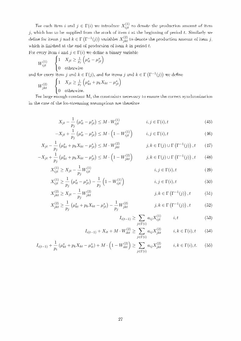
For each item i and j ∈ Γ(i) we introduce X(1)ijt to denote the production amount of item

j, which has to be supplied from the stock of item i at the beginning of period t. Similarly we

de�ne for items j and k ∈ Γ(Γ−1(j)

)variables X

(2)jkt to denote the production amount of item j,

which is �nished at the end of production of item k in period t.

For every item i and j ∈ Γ(i) we de�ne a binary variable

W(1)ijt

1 Xjt ≥ 1pj

(µsit − µsjt

)0 otherwise

and for every item j and k ∈ Γ(j), and for items j and k ∈ Γ(Γ−1(j)

)we de�ne

W(2)jkt

1 Xjt ≥ 1pj

(µskt + pkXkt − µsjt

)0 otherwise.

For large enough constant M, the constraints necessary to ensure the correct synchronization

in the case of the lot-streaming assumptions are therefore

Xjt −1pj

(µsit − µsjt

)≤M ·W (1)

ijt i, j ∈ Γ(i), t (45)

−Xjt +1pj

(µsit − µsjt

)≤M ·

(1−W (1)

ijt

)i, j ∈ Γ(i), t (46)

Xjt −1pj

(µskt + pkXkt − µsjt

)≤M ·W (2)

jkt j, k ∈ Γ(j) ∪ Γ(Γ−1(j)

), t (47)

−Xjt +1pj

(µskt + pkXkt − µsjt

)≤M ·

(1−W (2)

jkt

)j, k ∈ Γ(j) ∪ Γ

(Γ−1(j)

), t (48)

X(1)ijt ≥ Xjt −

1pjW

(1)ijt i, j ∈ Γ(i), t (49)

X(1)ijt ≥

1pj

(µsit − µsjt

)− 1pj

(1−W (1)

ijt

)i, j ∈ Γ(i), t (50)

X(2)jkt ≥ Xjt −

1pjW

(2)jkt j, k ∈ Γ

(Γ−1(j)

), t (51)

X(2)jkt ≥

1pj

(µskt + pkXkt − µsjt

)− 1pjW

(2)jkt j, k ∈ Γ

(Γ−1(j)

), t (52)

Ii(t−1) ≥∑j∈Γ(i)

aijX(1)ijt i, t (53)

Ii(t−1) +Xit +M ·W (2)ikt ≥

∑j∈Γ(i)

aijX(2)jkt i, k ∈ Γ(i), t (54)

Ii(t−1) +1pi

(µskt + pkXkt − µsit) +M ·(

1−W (2)ikt

)≥∑j∈Γ(i)

aijX(2)jkt i, k ∈ Γ(i), t. (55)

27