Fix-and-Optimize Heuristic and MP-based Approaches for Capacitated Lot Sizing

Problem with Setup Carryover, Setup Splitting and Backlogging

by

Cheng-Lung Chen

A Thesis Presented in Partial Fulfillmentof the Requirements for the Degree

Master of Science

Approved June 2015 by theGraduate Supervisory Committee:

Muhong Zhang, Co-ChairSrimathy Mohan, Co-Chair

Teresa Wu

ARIZONA STATE UNIVERSITY

August 2015

ABSTRACT

In this thesis, a single-level, multi-item capacitated lot sizing problem with setup carry-

over, setup splitting and backlogging is investigated. This problem is typically used in

the tactical and operational planning stage, determining the optimal production quantities

and sequencing for all the products in the planning horizon. Although the capacitated lot

sizing problems have been investigated with many different features from researchers, the

simultaneous consideration of setup carryover and setup splitting is relatively new. This

consideration is beneficial to reduce costs and produce feasible production schedule. Setup

carryover allows the production setup to be continued between two adjacent periods with-

out incurring extra setup costs and setup times. Setup splitting permits the setup to be

partially finished in one period and continued in the next period, utilizing the capacity more

efficiently and remove infeasibility of production schedule.

The main approaches are that first the simple plant location formulation is adopted

to reformulate the original model. Furthermore, an extended formulation by redefining

the idle period constraints is developed to make the formulation tighter. Then for the

purpose of evaluating the solution quality from heuristic, three types of valid inequalities

are added to the model. A fix-and-optimize heuristic with two-stage product decomposition

and period decomposition strategies is proposed to solve the formulation. This generic

heuristic solves a small portion of binary variables and all the continuous variables rapidly

in each subproblem. In addition, the case with demand backlogging is also incorporated to

demonstrate that making additional assumptions to the basic formulation does not require

to completely altering the heuristic.

The contribution of this thesis includes several aspects: the computational results show

the capability, flexibility and effectiveness of the approaches. The average optimality gap

is 6% for data without backlogging and 8% for data with backlogging, respectively. In

addition, when backlogging is not allowed, the performance of fix-and-optimize heuristic

is stable regardless of period length. This gives advantage of using such approach to plan

i

longer production schedule. Furthermore, the performance of the proposed solution ap-

proaches is analyzed so that later research on similar topics could compare the result with

different solution strategies.

ii

DEDICATION

To my grandma Jui-Hsun Yeh, who left us too early, your memory will always be in our

hearts.

iii

ACKNOWLEDGEMENTS

First and foremost I would like to dedicate my sincere gratitude to my thesis advisors

Dr. Muhong Zhang and Dr. Srimathy Mohan for giving me this opportunity to conduct

research with them. Thanks to their patience and continuous support, my knowledge have

been broadened and deepened, I have also acquired the essential attitude toward academic

research. Most importantly, I appreciate all their contribution of time and ideas to make

my research experience productive and stimulating. Without their guidance and persistent

help, this thesis would not have been possible.

I would also like to thank Dr. Teresa Wu for serving my thesis committee member and

sharing her invaluable comments and research experience with me. Besides them, I would

like to thank to all other professors who taught me many interesting topics to reinforce my

understanding in the field of industrial engineering and operations research, Dr. Ronald

Askin, Dr. Linda Chattin, Dr. Esma Gel, Dr. Jing Li, Dr. Pitu Mirchandani, Dr. Rong

Pan and Dr. Soroush Saghafian.

My time at Arizona State University was made enjoyable in large part because of the

many friends that became a part of my life. They helped me through the transition from

business to engineering and enabled me to obtain different perspective by discussing and

sharing ideas each other. Special thanks go to Peiyun Guo, Wei-Chieh Kao, Chao Li,

Xiaoyan Li, Jierui Liu, Lingling Ma, Polo Dening Peng, Yazhu Song and Tong Zhou, for

their encouragement and assistance during this thesis research process.

I also take this opportunity to thank my old friends Yu-Mei Tseng, Pin-Hsuan Lee, I-Yen

Tsai, Jui-Tung Hong, I-Ting Hsueh, Hui-Jin Wu, Yu-Ju Weng, Li-Chen Tu, Pei-Chun Cho,

Ai-Chen Chung, Cheng-Wei Chen and R2438 at SCU for their unconditional friendship even

though we are far apart from each other right now. True friendship means being separated

and nothing changes.

Finally, I would like to thank my parents Kun-Fu and Mei-Yu, my two younger sisters,

Ju-Lin and Ching-Hui for always believing my capability and giving all the support I need.

iv

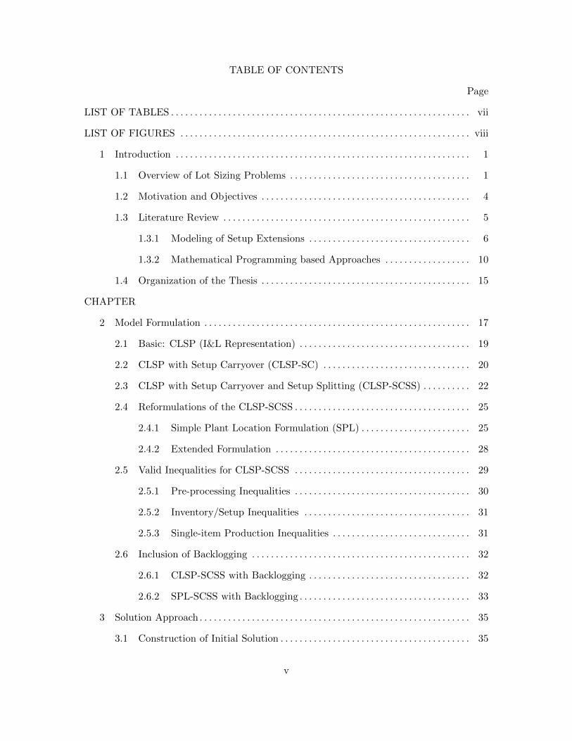
TABLE OF CONTENTS

Page

LIST OF TABLES . . . . . . . . . . . . . . . . . . . . . . . . . . . . . . . . . . . . . . . . . . . . . . . . . . . . . . . . . . . . . . . vii

LIST OF FIGURES . . . . . . . . . . . . . . . . . . . . . . . . . . . . . . . . . . . . . . . . . . . . . . . . . . . . . . . . . . . . . viii

1 Introduction . . . . . . . . . . . . . . . . . . . . . . . . . . . . . . . . . . . . . . . . . . . . . . . . . . . . . . . . . . . . . . 1

1.1 Overview of Lot Sizing Problems . . . . . . . . . . . . . . . . . . . . . . . . . . . . . . . . . . . . . . 1

1.2 Motivation and Objectives . . . . . . . . . . . . . . . . . . . . . . . . . . . . . . . . . . . . . . . . . . . . 4

1.3 Literature Review . . . . . . . . . . . . . . . . . . . . . . . . . . . . . . . . . . . . . . . . . . . . . . . . . . . . 5

1.3.1 Modeling of Setup Extensions . . . . . . . . . . . . . . . . . . . . . . . . . . . . . . . . . . 6

1.3.2 Mathematical Programming based Approaches . . . . . . . . . . . . . . . . . . 10

1.4 Organization of the Thesis . . . . . . . . . . . . . . . . . . . . . . . . . . . . . . . . . . . . . . . . . . . . 15

CHAPTER

2 Model Formulation . . . . . . . . . . . . . . . . . . . . . . . . . . . . . . . . . . . . . . . . . . . . . . . . . . . . . . . . 17

2.1 Basic: CLSP (I&L Representation) . . . . . . . . . . . . . . . . . . . . . . . . . . . . . . . . . . . . 19

2.2 CLSP with Setup Carryover (CLSP-SC) . . . . . . . . . . . . . . . . . . . . . . . . . . . . . . . 20

2.3 CLSP with Setup Carryover and Setup Splitting (CLSP-SCSS) . . . . . . . . . . 22

2.4 Reformulations of the CLSP-SCSS . . . . . . . . . . . . . . . . . . . . . . . . . . . . . . . . . . . . . 25

2.4.1 Simple Plant Location Formulation (SPL) . . . . . . . . . . . . . . . . . . . . . . . 25

2.4.2 Extended Formulation . . . . . . . . . . . . . . . . . . . . . . . . . . . . . . . . . . . . . . . . . 28

2.5 Valid Inequalities for CLSP-SCSS . . . . . . . . . . . . . . . . . . . . . . . . . . . . . . . . . . . . . 29

2.5.1 Pre-processing Inequalities . . . . . . . . . . . . . . . . . . . . . . . . . . . . . . . . . . . . . 30

2.5.2 Inventory/Setup Inequalities . . . . . . . . . . . . . . . . . . . . . . . . . . . . . . . . . . . 31

2.5.3 Single-item Production Inequalities . . . . . . . . . . . . . . . . . . . . . . . . . . . . . 31

2.6 Inclusion of Backlogging . . . . . . . . . . . . . . . . . . . . . . . . . . . . . . . . . . . . . . . . . . . . . . 32

2.6.1 CLSP-SCSS with Backlogging . . . . . . . . . . . . . . . . . . . . . . . . . . . . . . . . . . 32

2.6.2 SPL-SCSS with Backlogging . . . . . . . . . . . . . . . . . . . . . . . . . . . . . . . . . . . . 33

3 Solution Approach . . . . . . . . . . . . . . . . . . . . . . . . . . . . . . . . . . . . . . . . . . . . . . . . . . . . . . . . . 35

3.1 Construction of Initial Solution . . . . . . . . . . . . . . . . . . . . . . . . . . . . . . . . . . . . . . . . 35

v

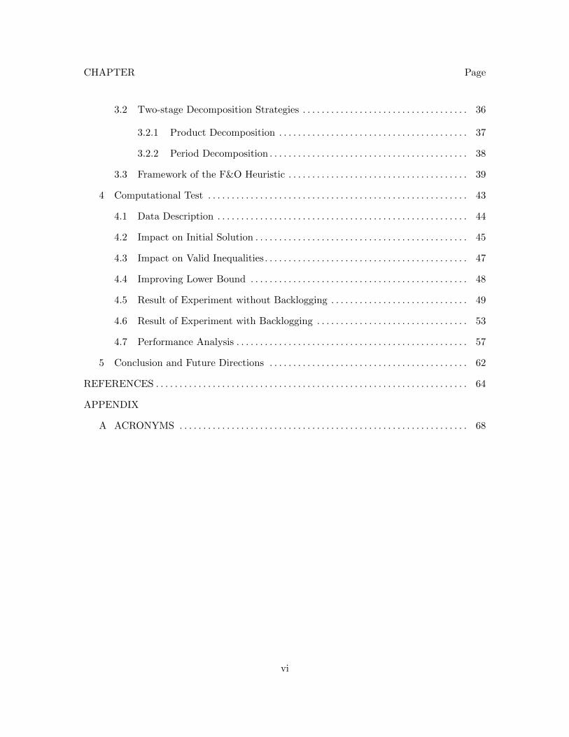
CHAPTER Page

3.2 Two-stage Decomposition Strategies . . . . . . . . . . . . . . . . . . . . . . . . . . . . . . . . . . . 36

3.2.1 Product Decomposition . . . . . . . . . . . . . . . . . . . . . . . . . . . . . . . . . . . . . . . . 37

3.2.2 Period Decomposition . . . . . . . . . . . . . . . . . . . . . . . . . . . . . . . . . . . . . . . . . . 38

3.3 Framework of the F&O Heuristic . . . . . . . . . . . . . . . . . . . . . . . . . . . . . . . . . . . . . . 39

4 Computational Test . . . . . . . . . . . . . . . . . . . . . . . . . . . . . . . . . . . . . . . . . . . . . . . . . . . . . . . 43

4.1 Data Description . . . . . . . . . . . . . . . . . . . . . . . . . . . . . . . . . . . . . . . . . . . . . . . . . . . . . 44

4.2 Impact on Initial Solution . . . . . . . . . . . . . . . . . . . . . . . . . . . . . . . . . . . . . . . . . . . . . 45

4.3 Impact on Valid Inequalities . . . . . . . . . . . . . . . . . . . . . . . . . . . . . . . . . . . . . . . . . . . 47

4.4 Improving Lower Bound . . . . . . . . . . . . . . . . . . . . . . . . . . . . . . . . . . . . . . . . . . . . . . 48

4.5 Result of Experiment without Backlogging . . . . . . . . . . . . . . . . . . . . . . . . . . . . . 49

4.6 Result of Experiment with Backlogging . . . . . . . . . . . . . . . . . . . . . . . . . . . . . . . . 53

4.7 Performance Analysis . . . . . . . . . . . . . . . . . . . . . . . . . . . . . . . . . . . . . . . . . . . . . . . . . 57

5 Conclusion and Future Directions . . . . . . . . . . . . . . . . . . . . . . . . . . . . . . . . . . . . . . . . . . 62

REFERENCES . . . . . . . . . . . . . . . . . . . . . . . . . . . . . . . . . . . . . . . . . . . . . . . . . . . . . . . . . . . . . . . . . . 64

APPENDIX

A ACRONYMS . . . . . . . . . . . . . . . . . . . . . . . . . . . . . . . . . . . . . . . . . . . . . . . . . . . . . . . . . . . . . 68

vi

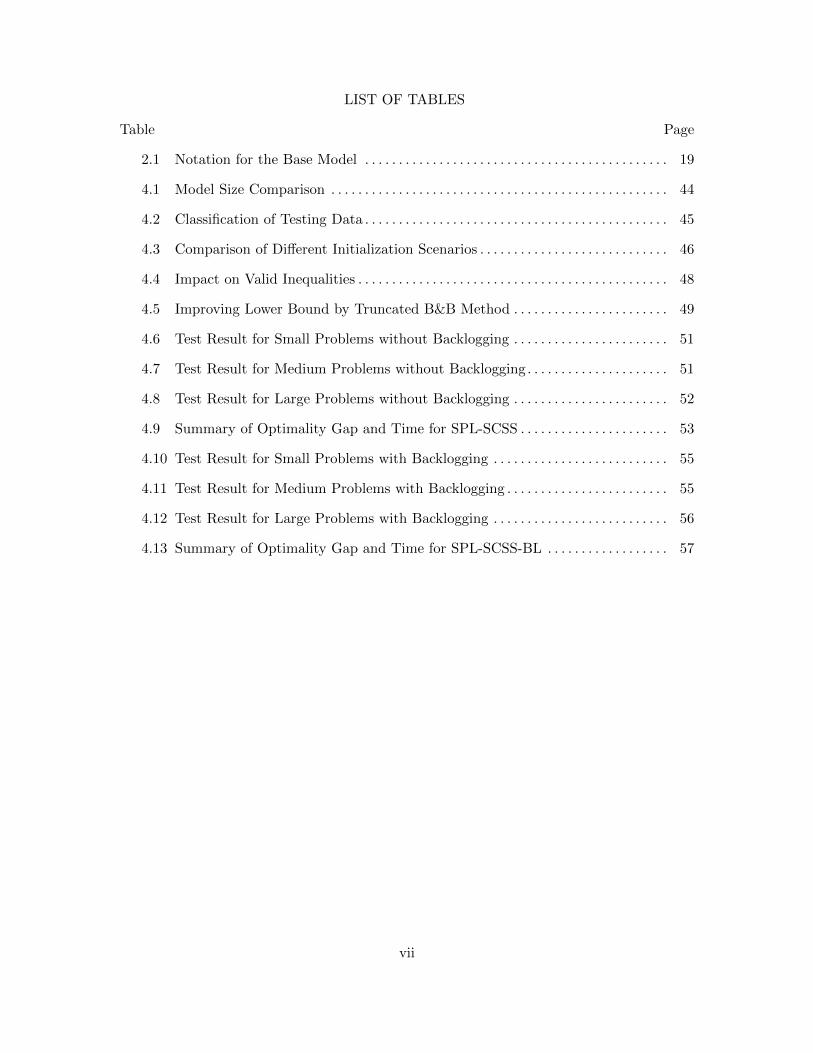
LIST OF TABLES

Table Page

2.1 Notation for the Base Model . . . . . . . . . . . . . . . . . . . . . . . . . . . . . . . . . . . . . . . . . . . . . 19

4.1 Model Size Comparison . . . . . . . . . . . . . . . . . . . . . . . . . . . . . . . . . . . . . . . . . . . . . . . . . . 44

4.2 Classification of Testing Data . . . . . . . . . . . . . . . . . . . . . . . . . . . . . . . . . . . . . . . . . . . . . 45

4.3 Comparison of Different Initialization Scenarios . . . . . . . . . . . . . . . . . . . . . . . . . . . . 46

4.4 Impact on Valid Inequalities . . . . . . . . . . . . . . . . . . . . . . . . . . . . . . . . . . . . . . . . . . . . . . 48

4.5 Improving Lower Bound by Truncated B&B Method . . . . . . . . . . . . . . . . . . . . . . . 49

4.6 Test Result for Small Problems without Backlogging . . . . . . . . . . . . . . . . . . . . . . . 51

4.7 Test Result for Medium Problems without Backlogging . . . . . . . . . . . . . . . . . . . . . 51

4.8 Test Result for Large Problems without Backlogging . . . . . . . . . . . . . . . . . . . . . . . 52

4.9 Summary of Optimality Gap and Time for SPL-SCSS . . . . . . . . . . . . . . . . . . . . . . 53

4.10 Test Result for Small Problems with Backlogging . . . . . . . . . . . . . . . . . . . . . . . . . . 55

4.11 Test Result for Medium Problems with Backlogging . . . . . . . . . . . . . . . . . . . . . . . . 55

4.12 Test Result for Large Problems with Backlogging . . . . . . . . . . . . . . . . . . . . . . . . . . 56

4.13 Summary of Optimality Gap and Time for SPL-SCSS-BL . . . . . . . . . . . . . . . . . . 57

vii

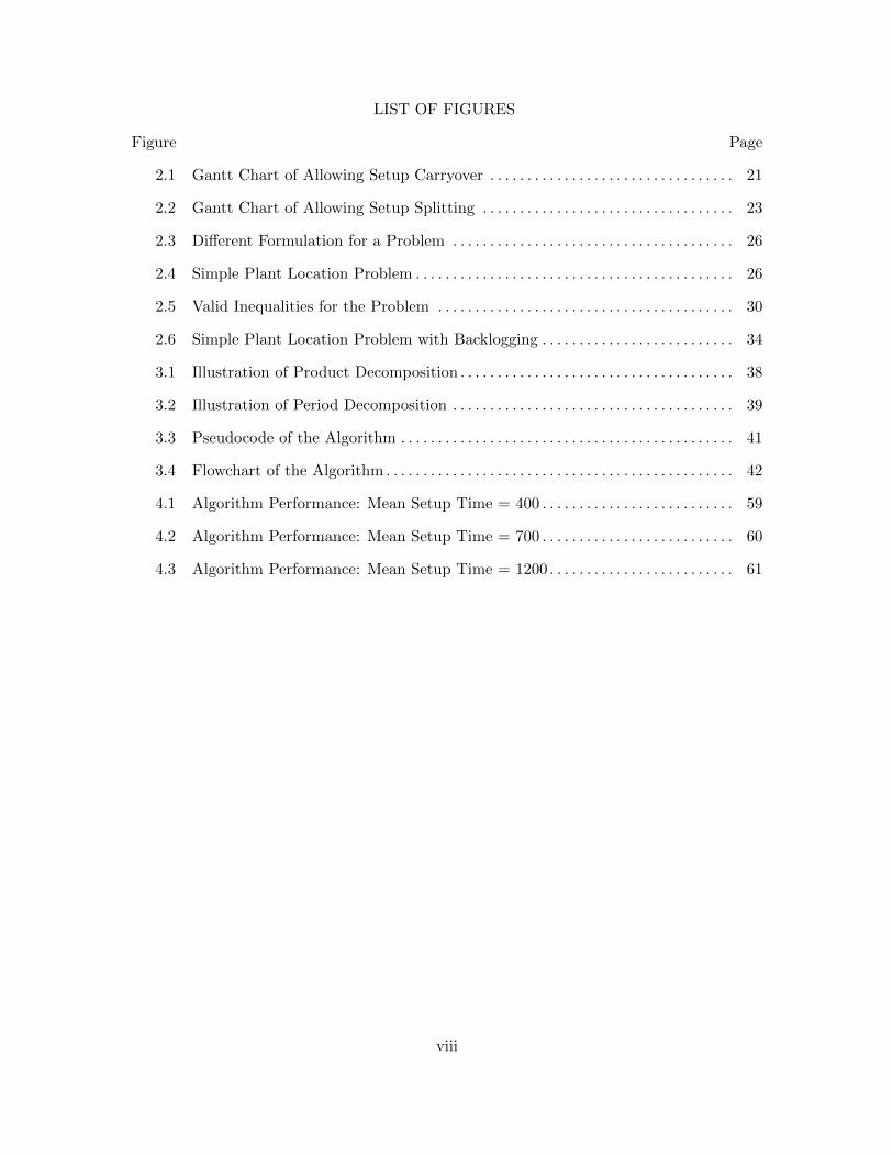
LIST OF FIGURES

Figure Page

2.1 Gantt Chart of Allowing Setup Carryover . . . . . . . . . . . . . . . . . . . . . . . . . . . . . . . . . 21

2.2 Gantt Chart of Allowing Setup Splitting . . . . . . . . . . . . . . . . . . . . . . . . . . . . . . . . . . 23

2.3 Different Formulation for a Problem . . . . . . . . . . . . . . . . . . . . . . . . . . . . . . . . . . . . . . 26

2.4 Simple Plant Location Problem . . . . . . . . . . . . . . . . . . . . . . . . . . . . . . . . . . . . . . . . . . . 26

2.5 Valid Inequalities for the Problem . . . . . . . . . . . . . . . . . . . . . . . . . . . . . . . . . . . . . . . . 30

2.6 Simple Plant Location Problem with Backlogging . . . . . . . . . . . . . . . . . . . . . . . . . . 34

3.1 Illustration of Product Decomposition . . . . . . . . . . . . . . . . . . . . . . . . . . . . . . . . . . . . . 38

3.2 Illustration of Period Decomposition . . . . . . . . . . . . . . . . . . . . . . . . . . . . . . . . . . . . . . 39

3.3 Pseudocode of the Algorithm . . . . . . . . . . . . . . . . . . . . . . . . . . . . . . . . . . . . . . . . . . . . . 41

3.4 Flowchart of the Algorithm . . . . . . . . . . . . . . . . . . . . . . . . . . . . . . . . . . . . . . . . . . . . . . . 42

4.1 Algorithm Performance: Mean Setup Time = 400 . . . . . . . . . . . . . . . . . . . . . . . . . . 59

4.2 Algorithm Performance: Mean Setup Time = 700 . . . . . . . . . . . . . . . . . . . . . . . . . . 60

4.3 Algorithm Performance: Mean Setup Time = 1200 . . . . . . . . . . . . . . . . . . . . . . . . . 61

viii

Chapter 1

INTRODUCTION

1.1 Overview of Lot Sizing Problems

Production planning and control is a recurring activity for manufacturing industry and

has remained one of the most challenging problems since the development of operations

research. Fast development in economics and globalization have elevated the level of com-

petition and continued to put pressure on corporations to squeeze out more productivity.

Under this situation, one of the key success strategies for manufacturing companies is to

achieve maximum efficiency and utility through the design of production processes. An

effective production planning demonstrates the ability of production system to produce

products at low costs with faster processes and minimum defective products. Generally, the

common objectives for production planning can be stated as the following: minimize total

production time and production costs, meet customer requirements and use resources effec-

tively. Depending on the type of production planning, mathematical models are extensively

adopted to support the decision making processes in this problem context.

Most production planning problems can be divided into three hierarchical stages: long-

term, medium-term and short-term planning. Decision making in long-term planning prob-

lems usually focus more on the strategic level of activities, such as facility location, selec-

tion of products and necessary equipment investment for production. While in medium-term

level, tactical planning decisions include allocation of capacity, determination of the amount

of overtime used and the amount of inventory. Short-term level planning usually involves

the production scheduling and sequencing of jobs for daily operations, vehicle routing and

inventory control activities. As one of the important components in production planning,

lot sizing attempts to determine the optimal timing and quantity of production for all the

products, so that the total cost of production can be minimized. To be more precise, the ex-

1

pected output of lot sizing is to give a complete picture of how many units of each product to

produce, and how many units to carry in inventory for each period in the planning horizon,

so that total relevant costs such as setup costs and inventory costs can be minimized. The

early development of lot sizing problem can be traced back to several decades ago. Harris

introduced the framework in 1913 for the well-known economical ordering quantity (EOQ)

model under the assumption of single-item, stationary demand and infinite planning hori-

zon (Harris, 1990, reprinted version). The model demonstrates a simple tradeoff between

order costs and inventory holding costs. Later the model was further analyzed and applied

extensively in practice. EOQ does not impose the capacity restriction, which was taken care

in the economic lot sizing problem (ELSP) (Rogers, 1958) as in reality the available resource

are limited. Starting from the Wagner-Whitin problem (Wagner and Whitin, 1958), named

after the two researchers who proposed this model, research direction has been shifted to

investigate lot sizing with time-varying demand and finite planning horizon.

Ever since then, lot sizing problem today has many extensions corresponding to different

assumptions and characteristics. Other than the type of demand data and length of planning

horizon, there are several characteristics of the lot sizing problem that deeply affect the

complexity. Production processes can be either be single-level or multi-level. Demand in

multi-level production has the predecessor-successor relationship, that is, the output of one

operation is the input of another. Capacity is another crucial factor in lot sizing. If the

limitation of capacity does not exist, the problem is called uncapacitated, otherwise it is

called capacitated. Problem with capacity limitation usually follows with setup time when

changeover of products is allowed during the production processes. For a setup to be done

within a time period, both setup cost and setup time can be either product-dependent or

sequence-dependent. If setup for a product is established in current period and carried

into next period to continue the production for similar product, it is often called setup

carryover or linked lot sizes. Setup carryover reduces additional setup costs and setup time,

thus giving lower cost production plans. It is also possible to perform setups between two

2

adjacent periods. This setup pattern is referred to as setup splitting or setup crossover

(Mohan et al., 2012; Belo-Filho et al., 2013). With setup splitting, period idle capacity can

be better utilized because inserting additional setups is possible. In terms of mathematical

modeling, whether to launch setups or not is modeled by binary variables, which makes

solving the problem even harder. Other features such as allowing demand backlogging or

using parallel machines in the production are considered in some lot sizing extensions as

well.

Since lot sizing can be classified according to different characteristics, they are commonly

divided into two groups: big bucket model and small bucket model. The fundamental

assumption for big bucket model is that it allows multiple items to be produced within

a single time period. Furthermore, setup operations can be performed multiple times as

needed. The time period in big bucket model usually represents the length of weeks or

months, so it can be used for medium-term planning. The capacitated lot sizing problem

(CLSP) is a typical big bucket model. CLSP allows multiple items to be produced with

capacity restrictions. The applicability and realistic assumption of CLSP to industrial

practice has triggered a lot of research over the past few decades. On the other hand, small

bucket model such as discrete lot sizing problem (DLSP) and continuous lot sizing problem

(CSLP), the former has a strict all-or-nothing assumption, indicating the production uses

up all capacity to produce one item only per period and incurs setup costs each time when

new lots are being produced. The later relaxes this relatively unrealistic condition and

allows setup to be preserved and carried into next few periods, resulting in less setup costs.

However, the unused capacity each period in CSLP is discarded, another small time bucket

model, the proportional lot sizing and scheduling problem (PLSP) allows the model to

schedule second item in some period if necessary. Because of the all-or-nothing assumption,

short-term daily operational planning usually considers small bucket model. In addition,

the solution output of small bucket model could provide production sequence information,

while the sequence is not obvious in big bucket model.

3

Solving lot sizing problem is a challenging task. Commercial production planning tools

such as material requirement planning (MRP) or manufacturing resource planning (MRP

II) aim to provide a solution for this routine problem. However, both MRP and MRP II

lack of certain features (Drexl and Kimms, 1997) so that they cannot satisfy the need from

practitioners. MRP does not consider the capacity constraints, whereas criticism for MRP

II usually lies in producing schedule with long lead times and backlogging. Researchers have

done a lot of investigation in favor of finding more sophisticated solution approaches for lot

sizing problems under different complicated assumptions. The computational complexity

for lot sizing problem such as ELSP or CLSP are known to be NP-hard (Florian et al.,

1980; Bitran and Yanasse, 1982; Hsu, 1983). Including different features into the model

will only increases the complexity. The theory of NP-completeness has reduced the hope

to solve NP-hard problem within polynomial computational times. Broadly speaking, no

dominant solution approaches has been proposed for lot sizing problems so far. Nevertheless,

effectively designed heuristic algorithm can be helpful in achieving nearly optimal solution

in a reasonable time.

1.2 Motivation and Objectives

One of the recent research trends on big bucket CLSP is to include setup carryover,

setup splitting and backlogging. Considering setup splitting either generates a better pro-

duction schedule in terms of lower costs or removes infeasibility from models with setup

carryover only. A possible condition for infeasibility is when the length of setup time is

substantially long and might even surpasses the capacity of the time period. Long setup

time is ubiquitous in some process manufacturing industries and automobile production

processes. Therefore it is necessary to take setup splitting into account in order to have

a feasible production schedule. In this thesis, we first study the single-level, multi-item,

capacitated lot sizing problem with setup carryover and setup splitting (CLSP-SCSS) and

then incorporate demand backlogging in the model. As an extension of the basic CLSP,

the CLSP-SCSS is also NP-hard. It is unlikely to solve the problem within reasonable time

4

limit by traditional exact methods such as branch-and-bound when problem size is getting

larger. To address this problem, the goal of this thesis is to focus on developing an efficient

solution procedure for the CLSP-SCSS. The contribution of this thesis is to give a compre-

hensive computational result for CLSP-SCSS and later other similar research can use our

work as a point of reference to compare the efficiency of different algorithms. In particular,

the objective of this research is to address the following questions.

• What are the factors that make setup splitting take effect?

• What is the overall performance of the proposed heuristic algorithm?

• How does the performance of the proposed algorithm affected by the characteristics

of the model, e.g. the number of products, periods, average length of setup time and

consideration of demand backlogging?

Reformulations and some valid inequalities are modified from previous research on the CLSP

with setup carryover, which can also be implemented if attempts are made to enhance

the mathematical formulation. Specifically, a MIP based heuristic called fix-and-optimize

heuristic is described and applied to solve the model with long average setup time (e.g.

120% of period capacity), large size data instances with number of 15 products and number

of periods 48.

In the following section, we give a detailed literature review on CLSP that considers

various types of setup operations, different characteristics and solution approaches. Then

we provide an outline to the rest of this thesis.

1.3 Literature Review

Research on capacitated lot sizing problem with different characteristics is plentiful. We

do not claim to cover every single article in this area. Therefore we restrict the review to

dynamic big bucket CLSP type with different setup operation features, i.e., setup carry-

over and setup splitting. We refer some excellent research work for reviews with possible

5

extensions of CLSP. For instance, Drexl and Kimms (1997) gave a comprehensive survey

on dynamic, capacitated lot sizing and scheduling. Karimi et al. (2003) discussed the sing-

level lot sizing together with exact method and heuristic algorithm. Gicquel et al. (2008)

reviewed the single and multi-level lot sizing on single or multiple resources. They also in-

cluded exact method, specialized heuristic, mathematical programming based heuristic and

meta-heuristic. Quadt and Kuhn (2008) presented a review for CLSP with several features

such as backlogging, setup carryover, sequencing and parallel machines. Similarly, various

solution approaches have been proposed to tackle CLSP. Our review focus on mathemati-

cal programming based approaches, especially the LP based heuristic. Jans and Degraeve

(2007) provided an overall review of lot sizing problem solved by meta-heuristic. Buschkuhl

et al. (2010) gave an excellent comprehensive review of multi-level capacitated lot sizing

problem (MLCLSP) on both modeling approach and corresponding algorithms during the

past four decades. Dıaz-Madronero et al. (2014) presented a survey work of 250 articles in

the domain of discrete-time tactical production planning. They classified these papers by

various attributes, including problem type, production structure, model extensions, solution

approaches, modeling languages and application filed. They concluded that master produc-

tion scheduling with a big bucket is the most widely studied problem type. In addition,

they highlighted that backlogging, setup time, parallel machines, overtime and network

formulation for model extension being considered the most.

1.3.1 Modeling of Setup Extensions

Two different important setup features have been considered in the capacitated lot sizing

problems: setup carryover and setup splitting. We begin to review these features in the

following sections and discuss their relation with this thesis.

Setup Carryover

The optimal production schedule from CLSP with setup carryover (CLSP-SC), or known

as CLSP with linked lot sizes (CLSPL) could be really different from CLSP. Production

6

for a specific item in previous period is continued to next period without additional setups,

thus saving the setup costs. Free capacity at the end of previous period is also possible to

be utilized as a setup for the immediate production in the next period.

Dillenberger et al. (1993) is known to be the first one to cover setup carryover in the

CLSP. Instead of considering holding costs or setup costs, the objective is to minimize total

weighted processing time and backlog units at the end of planning horizon. Also, in their

formulation setups can be carried over several periods.

Haase (1994) established the name linked lot sizes for the standard CLSP. The so-called

CLSPL considers production on a single resource without setup time. The objective is to

minimize total holding and setup costs. Similar to Dillenberger et al. (1993), the formulation

allows consecutive setup carryover. Later in Haase (1998), he reduced the formulation and

restricted setup can only be carried over at most one period.

Gopalakrishnan et al. (1995) proposed two types of single resource CLSPL. The first

formulation takes product-independent setup time and setup costs into account. Compare

to previous research, binary variables are used extensively to model setup carryover. Setup

preserved over idle periods is indicated by auxiliary variables. The objective is to minimize

total holding and setup costs. The author referred second formulation as an integrated

model, which it includes attributes such as parallel machines, resource assignment and tool

selection. Gopalakrishnan (2000) modified the first model of CLPSL in Gopalakrishnan

et al. (1995) by incorporating producti-dependent setup time and setup costs.

Sox and Gao (1999) considered CLSPL on a single resource with product-dependent

setup costs, holding costs and variable production costs but without setup time. They also

restricted the number of setup carryover to be one across two periods.

Suerie and Stadtler (2003) allowed setup can be carried over several consecutive periods

in CLSPL and then extended it as to a multi-level production structure (MLCLSPL). They

also assumed production happened on multiple resources with a unique assignment to each

resource for every product.

7

Gupta and Magnusson (2005) developed a single resource CLSPL with sequence-dependent

setup costs and setup time. Here again setups can be carried over several periods. Their for-

mulation is similar to Gopalakrishnan et al. (1995). The sequence-dependency relationship

gives the sequence of products in every period.

Quadt and Kuhn (2009) presented a CLSPL with setup time, backlogging and parallel

machines. A subsequent model provides sequence and schedule of products on parallel

machines. Their research is motivated from the semiconductor assembly facility.

Setup Splitting

Modeling setup splitting is necessary for some manufacturing industry that the portion of

setup time is considerably long and capacity is scarce.

In the two small bucket PLSP based formulations, Suerie (2006) clearly defined the

starting and ending points of setup operations to handle long setup times. He solved the in-

stances by commercial MIP solver with additional valid inequalities, providing improvement

on solution quality compared with Drexl and Haase (1995).

Sung and Maravelias (2008) incorporated sequence independent setups, non-uniform

time buckets and long setup time in their formulation, as these features are often founded

in process manufacturing industry. They took the solutions without setup carryover and

crossover and adjusted the time bucket boundaries to handle long setup time by allowing

setup carryover and crossover. They also gave detail description to include idle time, parallel

machines, families of products, backlogged demand and lost of sales in the formulation.

Menezes et al. (2011) considered sequence-dependent, non-triangular setup, setup carry-

over and crossover in CLSP. The sequence-dependent feature may result in producing more

than one batch for a similar product within a period. They introduced a dynamical method

to omit disconnected sub tours, as this is especially important for large problems. The

computational test showed that setup crossover is important for obtaining better solution

compared with small bucket models.

8

Kopanos et al. (2011) developed a formulation for simultaneous production planning and

scheduling, where items are grouped into families. They allowed the changeover of families

to be crossover two adjacent periods and applied the model on a large-scale industrial case.

The result indicated that the formulation works well since hundred of items could be solved

in a reasonable time.

Mohan et al. (2012) presented a single-level single machine CLSP-SCSS, which is an

extended formulation of CLSPL from Suerie and Stadtler (2003). They included variables

to indicate start and finish time when splitting occurs. Based on a small numerical test,

they demonstrated that solutions obtained from CLSP-SCSS are either at least equal or

better than CLSPL. Furthermore, CLSP-SCSS could find solutions in instances that are

considered infeasible in CLSPL.

Belo-Filho et al. (2013) proposed two formulations that involve backlogged demand,

setup carryover and setup crossover. The first formulation is based on Sung and Maravelias

(2008) and reformulated in simple plant location representation. The second uses the dis-

aggregated time-index approach by defining starting and ending point on all the setup

operations, resulting in less integer variables. The computational results showed that setup

crossover is essential and uses the idle time more efficiently when setup time consumes a

significant portion of period capacity.

Fiorotto et al. (2014) took the ideas from Menezes et al. (2011) and Mohan et al. (2012)

and reformulate two models in simple plant location with setup crossover only. They devel-

oped three methods to model setup crossover without using extra binary variables. More-

over, they added symmetry breaking constraints on two literature models to analyze the

relationship among these formulations. The computational test was conducted on instances

taken from Trigeiro et al. (1989) and they concluded in two aspects: setup crossover is

especially worth to have when backlog is allowed and more feasible solutions could be found

with the existence of setup crossover.

9

Summary

From the literature, research consider setup carryover have attracted much attentions. The

assumption of allowing setup carryover is more realistic and provide cost-attractive produc-

tion schedule. Therefore other extensions such as parallel machines, backlogging, multi-level

structure as well as many solution approaches have been investigated. On the other hand,

unlike the flourish research of CLSP-SC and its variants, the number of literature of CLSP

with setup splitting is relatively limited. By far research trend on setup splitting is mainly

emphasizing in the formulation technique. The computational test results are based on

imposing time limit for MIP solver to evaluate the optimality gap between different formu-

lations. No literature regarding to specific solution technique to handle CLSP with setup

splitting have been proposed so far. This thesis aims to provide a computational study and

fill this gap in.

1.3.2 Mathematical Programming based Approaches

The property of mathematical programming based approaches is that they are more

flexible and general than other solution approaches when it comes to model extensions.

This group can be divided into exact method and LP-based heuristic. Since most of the lot

sizing problems are NP-hard, heuristic technique are adopted to solve the problem. Exact

method such as brand and bound (B&B) enumerates feasible solutions in the whole solution

space. Although B&B guarantees to find an optimal solution if it exists, the required

computational time would be too long if the problem size is large. While heuristic only

examine partial solution space and try to return a good quality solution in a reasonable

time. Research trend on solution approaches of lot sizing is either trying to develop a

faster heuristic algorithm that leads to nearly optimal solution or combing several different

solution techniques together to increase the overall efficiency. This research adopts several

mathematical programming based approaches hence we give a review focus on this group.

10

Reformulations

The efficiency of standard MIP solver is heavily depending on the mathematical formula-

tion. The technique of reformulations redefines the variable and seeks to approximate the

convex hull of the integer programming model. Moreover, reformulations are often used

to increase the efficiency for standard MIP solver and to tighten the LP relaxation since

the bound generated from LP relaxation of CLSP are often very loose. Two reformulation

techniques have been proposed so far. Eppen and Martin (1987) introduced the short-

est route (SR) formulation for standard CLSP. Tempelmeier and Helber (1994) included

capacity constraints and multi-level structure in this formulation. Stadtler (1996, 1997) pro-

posed a improved SR formulation for MLCLSP with reducing some constraints in contrast

to Tempelmeier and Helber (1994). Another reformulation is called simple plant location

(SPL) formulation. Rosling (1986) first introduced it to model a multi-level uncapacitated

lot sizing problem, which is an extension of Krarup and Bilde (1977). Later Maes et al.

(1991) added capacity constraints to it. Stadtler (1996) again proposed a SPL formulation

for a general bill-of-material structure. The author observed that the LP bound for both

formulations is identical. This observation is proved in Denizel et al. (2008)such that LP

bound of both SR and SPL for CLSP with setup time are exactly the same.

Valid Inequalities

A common way to tighten the formulation is by adding valid inequalities so the irrelevant

part of solution space can be cutoff. The success of dealing traveling salesman problem

by cutting plane method in 1980 has motivated researchers to develop problem-specific

valid inequalities for lot sizing problems as well (Pochet and Wolsey, 2006). Barany et al.

(1984) derived valid inequalities to describe the convex hull for single-item uncapacited lot

sizing problem. Miller et al. (2000) considered the capacitated case. Another extension on

multi-item based on Barany et al. (1984) is made by Pochet and Wolsey (1991). Belvaux

and Wolsey (2000) presented a framework called bc-prod to generate pre-processing, lot

11

sizing specific inequalities and general cutting plane lot sizing problems. Later in Belvaux

and Wolsey (2001) they included cases with start-up, changeover and switch off conditions.

Suerie and Stadtler (2003) extended the MLCLSPL formulation by making the idle-period

indicator variables from time-dependent become product-dependent. Three set of valid

inequalities were embedded to the branch-and-cut or cut-and-branch processes for finding

first feasible solution, so heuristic can use it as a starting point.

Rounding Heuristic

Many research on lot sizing problems use rounding heuristic (RH) to generate initial feasible

solution, it belongs to constructive heuristic. After solving the LP relaxation, the fractional

binary variables are rounded afterwards. With the capacity constraints, the setup patterns

might not be feasible if backlogging or overtime is not allowed. However, the solution can

serve as a starting point and combined with other heuristic. Eppen and Martin (1987)

introduced RH with B&B together to solve the SR formulation of CLSP. Maes et al. (1991)

presented some RH to solve the SPL formulation of MLCLSP without considering setup

time. Akartunalı and Miller (2009) combined RH and relax-and-fix (see next section) to

solve MLCLSP with valid inequalities added. The RH is used to determine initial feasible

solution and upper bound cutoff values for later window, the experiment showed that it

improved the solution process.

Relax-and-fix Heuristic

Relax-and-fix (R&F) heuristic divide the binary variables into three subsets, resulting in less

binary to be treated simultaneously hence reducing the computational effort. The binary

variables are fixing at current value, relaxing to continuous value or solving to optimality

in the given interval. Dillenberger et al. (1993) applied R&F heuristic with B&B algorithm

for the CLSPL. The binary setup variables are fixed to all the prior periods and relaxed to

current periods until the end of planning horizon. The branching order is determined by the

sequence of periods. Stadtler (2003) proposed a overlapping rolling time window heuristic

12

for MLCLSP. The length of time window, later period where binary variables are relaxed

and number of overlapping periods when move to next iteration are controlled by separate

parameters. As the planning time window move forward, the setup variables are optimized

except the last period in current window is relaxed. Also, binary in previous time windows

are all fixed except the overlapping periods. This method is also used in Suerie and Stadtler

(2003) for the MLCLSPL. Federgruen et al. (2007) also adopted R&F for the CLSP with

joint setup costs.

Fix-and-optimize Heuristic

The general idea of fix-and-optimize (F&O) heuristic is to decompose the binary variables

into two disjoint sets K and L. A subproblem consists of the set K to be fixed, while the set

L and all other continuous variables are optimized in the algorithm in an iterative manner.

Given an initial solution, the algorithm update the incumbent solution in each iteration

whenever better solution is found until the terminating condition is met.

Sahling et al. (2009) first proposed the iterative F&O heuristic for the multi-level capac-

itated lot sizing problem with setup carryover (MLCLSPL). They presented three principles

to determine the search direction in the solution space and relative number of binary vari-

ables optimized for the heuristic: product decomposition, resource decomposition and pro-

cess decomposition. Their experiment showed the cost of each product affect the solution

founded by the heuristic therefore they presented a cost-approximation formula to decide

the product decomposition order. They concluded that the selection of subset of products

and periods is a critical part for the heuristic. Later in Helber and Sahling (2010), they

applied the same F&O approach again for the multi-level case with lead time. They pointed

out that one could obtain higher solution quality with unfixing more binary variables in the

algorithm.

Goren et al. (2012) embedded the F&O heuristic into the genetic algorithm for the

capacitated lot sizing problem with setup carryover. Unlike Sahling et al. (2009) and Helber

and Sahling (2010) set all the setup variables to construct an initial solution, they used GA

13

to determine the initial solution then applied F&O heuristic to guide the GA jump out from

local minima to new solution space. They compared the result with Gopalakrishnan et al.

(2001) and using pure GA only. Overall the proposed hybrid approach is out performed the

others.

Lang and Shen (2011) considered the capacited lot sizing problem with sequence-dependent

setups and substitutions (CLSD-S) by using Relax-and-Fix (R&F) and F&O heuristic. The

initial fixation of all setup variables does not always guarantee a feasible solution in the

CLSD-S. They took the idea from Asymmetric Traveling Salesman Problem to determine

the efficient product sequence for generating initial solution. The computational results

showed that F&O approach combined with time window decomposition is better then prod-

uct decomposition. Furthermore the F&O approach surpasses the R&F approach.

Xiao et al. (2013) examined CLSP with sequence-dependent setup time (CLSD), time

window, machine eligibility and preference constraints. They applied fix-and-optimize to

solve the problem based on a decomposition strategy called randomized lease flexible rule,

which fixed the binary variables with the assignment of machines. The computational ex-

periment demonstrated that this strategy improve the previous fix-and-optimize algorithm

especially for data with high machine flexibility and demand variation.

Summary

Generally, mathematical programming based approaches provide two aspects for solving

the problem: the constructive phase and improvement phase. First, in the process of

constructive heuristic, one can simply impose a time limit in the branch-and-bound process

to obtain a solution, using this initial solution as a starting point. The purpose is to generate

a good quality initial solution and hopefully it would lead to good suboptimal or even true

optimal solution. However, the solution quality is highly depending on the formulation.

Reformulation technique and valid inequalities help reduce the feasible solution space but

still include all feasible integer solutions. Using rounding heuristic is intuitive and easy to

implement, however, the rounded setup variables might not be able to generate a feasible

14

schedule as the capacity might be violated. Including overtime in the model can solve this

problem. R&F heuristic also seek to generate a initial feasible solution by using rolling

time window, however, Helber and Sahling (2010) pointed out the implementation of R&F

heuristic used in Stadtler (2003) is quite time-consuming and often fail to find first feasible

solution within the given time limit.

Secondly, improvement heuristic such as F&O heuristic divides the solution space into

different neighborhoods. The solution moves from one neighborhood to another for ob-

taining better solution in the iterative procedure until reach the local optimum. Recall

the time-consuming issue mentioned about R&F above, F&O does not have such disad-

vantage, as in each iteration all the continuous variable are optimized with a small subset

of setup binary variables, the capacity infeasibility can be removed quickly. Because the

F&O only considers the subset of binary variables and treats all the continuous variables

equally, adding extra constraints without modifying the procedure is possible. The flexi-

bility of implementation also allow F&O to be embedded to other algorithm or combine

it with other methods. It is worth to understand the initial solution, the size of K and L

and the decomposition strategies are all crucial factors to effect the computational time and

solution quality of F&O algorithm.

Given the analysis mentioned of each method above, we combine the reformulations,

valid inequalities ,rounding heuristic to construct a good initial solution and fix-and-optimize

heuristic together to solve the problem.

1.4 Organization of the Thesis

The remainder of this thesis is organized as follows. Chapter 2 includes the standard

formulation of CLSP and then discuss the extension with setup carryover and setup splitting,

respectively. A reformulation of CLSP-SCSS based on the simple plant location (SPL-SCSS)

representation is presented. We also introduce the extended formulation and three sets of

valid inequalities are modified specifically for SPL. The last section of this chapter describes

the modification of allowing backlogging to the model both in standard formulation and

15

simple plant location representation. In chapter 3, we describe the implementation of fix-

and-optimize heuristic, including the selection of initial feasible solution and two types of

decomposition methods: product and period decomposition. Chapter 4 gives the results

and analysis of computational test. As summarized in chapter 5, our studies promote the

effectiveness of using the chosen heuristic together with mathematical-programming based

approaches to solve CLSP-SCSS. We also suggest further research on applying different

algorithms to improve or solve the extension of this problem.

16

Chapter 2

MODEL FORMULATION

In this chapter we present the basic formulation of single-level, multi-products capacitated

lot sizing problems and its two extensions: the capacitated lot sizing problem with setup

carryover (CLSP-SC) and the capacitated lot sizing problem with setup carryover and setup

splitting (CLSP-SCSS). CLSP-SCSS is the base formulation to solve problem, later we

reformulate CLSP-SCSS by using simple plant location formulation SPL-SCSS to estimate

the lower bound. Valid inequalities are developed to SPL-SCSS. The final section gives the

necessary modification of allowing backlogging to both basic and strengthened formulation.

We first discuss the characteristic and general assumption of the model.

• A set of different products {1,...,N} is manufactured on a single resource and the

production processes is assumed to be single level.

• For a single level production processes, there is no successor of the end item. Ini-

tial inventory and ending inventory are assumed to be zero. In practical continuous

and multi-level production environment, initial inventory and ending inventory are

considered in each stage. We simplify the assumption here.

• Excessive items produced are stored as inventory and incur inventory costs.

• Planning horizon is divided into several discrete time periods {1,..,T}.

• Both setup time and setup costs are product-dependent, setups consume capacity and

incur setup costs.

• The demand of each product is time-variant. For data without backlogging, zero

demand are inserted in the first several periods to ensure the feasibility. Such modi-

fication is not required for data with backlogging.

17

• Overtime production is allowed and incurs penalty costs if period capacity is not

sufficient. In practice, a production schedule with overtime is never desired . We

include the overtime to indicate whether the solution output gives an acceptable

schedule without generating high penalty costs.

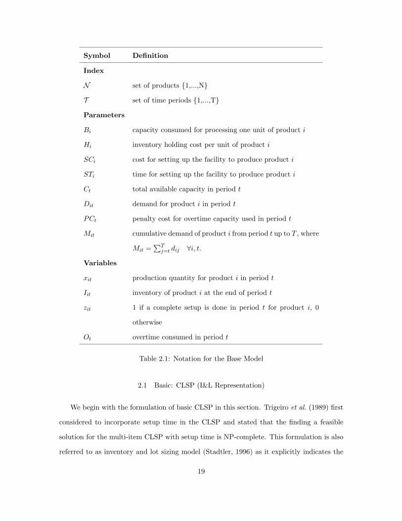
The symbols and notation used in the formulation of the next couple of sections is presented

in Table 2.1.

18

Symbol Definition

Index

N set of products {1,...,N}

T set of time periods {1,...,T}

Parameters

Bi capacity consumed for processing one unit of product i

Hi inventory holding cost per unit of product i

SCi cost for setting up the facility to produce product i

STi time for setting up the facility to produce product i

Ct total available capacity in period t

Dit demand for product i in period t

PCt penalty cost for overtime capacity used in period t

Mit cumulative demand of product i from period t up to T , where

Mit =∑T

j=t dij ∀i, t.

Variables

xit production quantity for product i in period t

Iit inventory of product i at the end of period t

zit 1 if a complete setup is done in period t for product i, 0

otherwise

Ot overtime consumed in period t

Table 2.1: Notation for the Base Model

2.1 Basic: CLSP (I&L Representation)

We begin with the formulation of basic CLSP in this section. Trigeiro et al. (1989) first

considered to incorporate setup time in the CLSP and stated that the finding a feasible

solution for the multi-item CLSP with setup time is NP-complete. This formulation is also

referred to as inventory and lot sizing model (Stadtler, 1996) as it explicitly indicates the

19

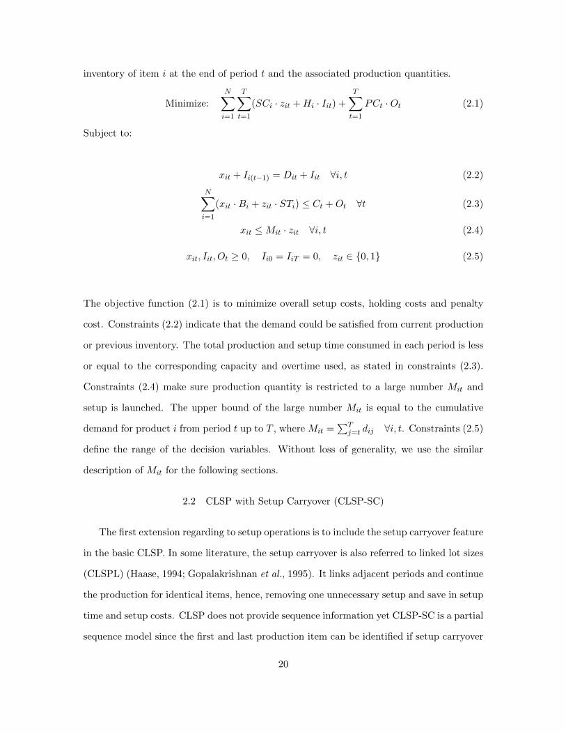
inventory of item i at the end of period t and the associated production quantities.

Minimize:N∑i=1

T∑t=1

(SCi · zit +Hi · Iit) +T∑t=1

PCt ·Ot (2.1)

Subject to:

xit + Ii(t−1) = Dit + Iit ∀i, t (2.2)

N∑i=1

(xit ·Bi + zit · STi) ≤ Ct +Ot ∀t (2.3)

xit ≤Mit · zit ∀i, t (2.4)

xit, Iit, Ot ≥ 0, Ii0 = IiT = 0, zit ∈ {0, 1} (2.5)

The objective function (2.1) is to minimize overall setup costs, holding costs and penalty

cost. Constraints (2.2) indicate that the demand could be satisfied from current production

or previous inventory. The total production and setup time consumed in each period is less

or equal to the corresponding capacity and overtime used, as stated in constraints (2.3).

Constraints (2.4) make sure production quantity is restricted to a large number Mit and

setup is launched. The upper bound of the large number Mit is equal to the cumulative

demand for product i from period t up to T , where Mit =∑T

j=t dij ∀i, t. Constraints (2.5)

define the range of the decision variables. Without loss of generality, we use the similar

description of Mit for the following sections.

2.2 CLSP with Setup Carryover (CLSP-SC)

The first extension regarding to setup operations is to include the setup carryover feature

in the basic CLSP. In some literature, the setup carryover is also referred to linked lot sizes

(CLSPL) (Haase, 1994; Gopalakrishnan et al., 1995). It links adjacent periods and continue

the production for identical items, hence, removing one unnecessary setup and save in setup

time and setup costs. CLSP does not provide sequence information yet CLSP-SC is a partial

sequence model since the first and last production item can be identified if setup carryover

20

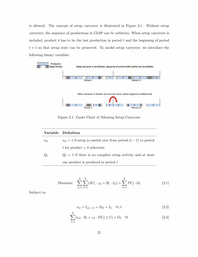
is allowed. The concept of setup carryover is illustrated in Figure 2.1. Without setup

carryover, the sequence of productions in CLSP can be arbitrary. When setup carryover is

included, product 4 has to be the last production in period t and the beginning of period

t + 1 so that setup state can be preserved. To model setup carryover, we introduce the

following binary variables.

Figure 2.1: Gantt Chart of Allowing Setup Carryover

Variable Definition

uit uit = 1 if setup is carried over from period (t− 1) to period

t for product i, 0 otherwise

Qt Qt = 1 if there is no complete setup activity and at most

one product is produced in period t

Minimize:N∑i=1

T∑t=1

(SCi · zit +Hi · Iit) +

T∑t=1

PCt ·Ot (2.1)

Subject to:

xit + Ii(t−1) = Dit + Iit ∀i, t (2.2)

N∑i=1

(xit ·Bi + zit · STi) ≤ Ct +Ot ∀t (2.3)

21

xit ≤Mit · (zit + uit) ∀i, t (2.6)

N∑i=1

uit ≤ 1 ∀t (2.7)

uit ≤ zi(t−1) + ui(t−1) ∀i, t (2.8)

zit +Qt ≤ 1 ∀i, t (2.9)

ui(t+1) + uit ≤ 1 +Qt ∀i, t (2.10)

xit, Iit, Ot, Qt ≥ 0, Ii0 = IiT = 0, ui1 = 0, zit, uit ∈ {0, 1} (2.11)

The definition of objective function (2.1), inventory balance constraints (2.2) and capacity

balance constraints (2.3) do not change in CLSP-SC. Constraints (2.6) restrict the produc-

tion quantity to cumulative demand Mit such that setup is launched or carried from previous

period. Constraints (2.7) secure that setup could be carried across over two periods for at

most one item only. Constraints (2.8) state that setup can be carried from period t− 1 to t

only if there is a complete setup in period t− 1 or setup is already carried over in t− 1. In

(2.9), Qt is the idle period indicator so that it is mutually exclusive with the complete setup

variables zit. Note here Qt does not have to declare as binary variables. Constraints (2.10)

make sure that setup can be carried over two consecutive periods if Qt = 1. Constraints

(2.11) define the range of the decision variables.

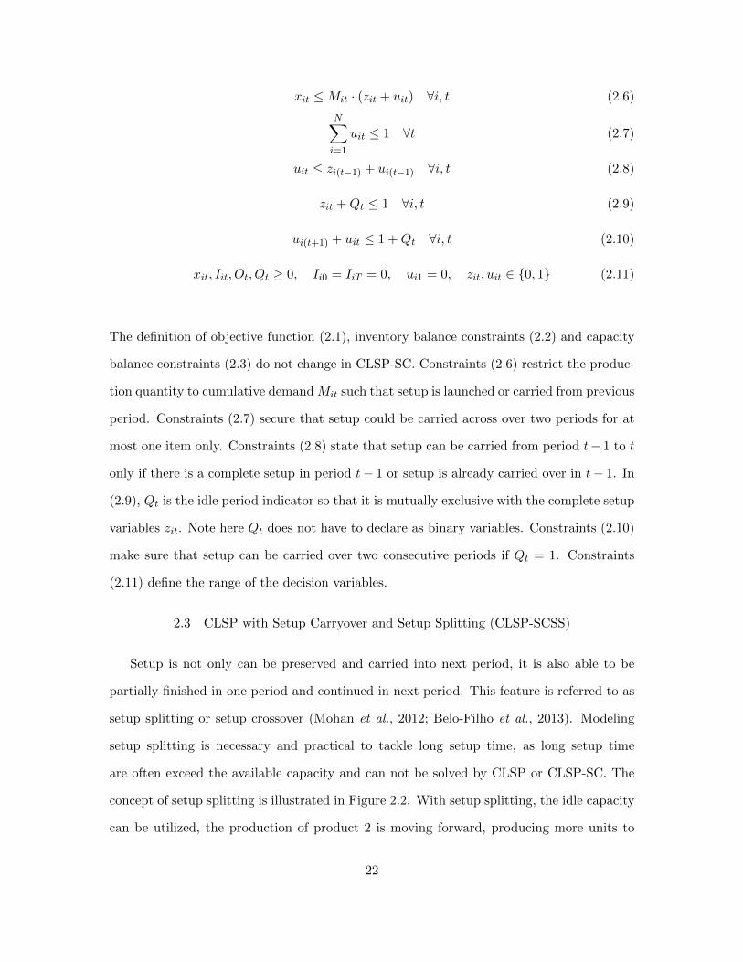
2.3 CLSP with Setup Carryover and Setup Splitting (CLSP-SCSS)

Setup is not only can be preserved and carried into next period, it is also able to be

partially finished in one period and continued in next period. This feature is referred to as

setup splitting or setup crossover (Mohan et al., 2012; Belo-Filho et al., 2013). Modeling

setup splitting is necessary and practical to tackle long setup time, as long setup time

are often exceed the available capacity and can not be solved by CLSP or CLSP-SC. The

concept of setup splitting is illustrated in Figure 2.2. With setup splitting, the idle capacity

can be utilized, the production of product 2 is moving forward, producing more units to

22

satisfy the demand. Also, if the setup activity exceeds the capacity, the setup splitting

allows possibility to perform the setups in two adjacent periods. Setup splitting is allowed

to be carried over to the next period if needed. To model the setup splitting feature, several

variables are added to the formulation.

Figure 2.2: Gantt Chart of Allowing Setup Splitting

Variable Definition

lit duration of the setup for product i completed at the end of

period t

fit duration of the setup for product i completed at the begin-

ning of period t

vit vit = 1 if setup is split between period (t − 1) and period t

for product i with the splits being li(t−1) and fit respectively,

0 otherwise

Minimize:

N∑i=1

T∑t=1

SCi · (zit + vit) +

N∑i=1

T∑t=1

Hi · Iit +

T∑t=1

PCt ·Ot (2.12)

23

Subject to:

xit + Ii(t−1) = Dit + Iit ∀i, t (2.2)

zit +Qt ≤ 1 ∀i, t (2.9)

ui(t+1) + uit ≤ 1 +Qt ∀i, t (2.10)

N∑i=1

(xit ·Bi + zit · STi + fit + lit) ≤ Ct +Ot ∀t (2.13)

xit ≤Mit · (zit + uit + vit) ∀i, t (2.14)

fit + li(t−1) = vit · STi ∀i, t (2.15)

N∑i=1

(uit + vit) ≤ 1 ∀t (2.16)

uit ≤ zi(t−1) + ui(t−1) + vi(t−1) ∀i, t (2.17)

ui(t+1) + vit ≤ 1 +Qt ∀i, t (2.18)

zit + uit + vit ≤ 1 ∀i, t (2.19)

xit, Iit, Ot, Qt, fit, lit ≥ 0, Ii0 = IiT = 0, ui1 = vi1 = 0, zit, uit, vit ∈ {0, 1} (2.20)

The definition of inventory balance constraints (2.2), idle period indication constraints (2.9)

and two-periods carryover constraints (2.10) are similar to previous section. Here the ob-

jective function (2.12) minimizes the total holding costs, penalty costs and setup costs with

the corresponding complete setup and setup splitting. Constraints (2.13) ensure that the

capacity consumed by production and setups is less or equal to available capacity and over-

time used in a period. Constraints (2.14) allow production activity only if either complete

setup, setup carryover or setup splitting is done in a period. Constraints (2.15) ensure that

the setup splitting time is the sum of two splitting indicator variables. Constraints (2.16)

state that either one setup carryover or setup splitting is allowed for at most one product

in a period. Constraints (2.17) make sure that setup carryover can only be done in period

24

t if there is either a complete setup or setup carryover or setup splitting in period t − 1.

Constraints (2.18) indicates that in an idle period, at most one product is being produced

because of partially setup and this setup state can be carried into next period. For each

production activity, constraints (2.19) ensure that only one setup condition (complete, car-

ryover or splitting) or no production in that period. Constraints (2.20) define the range of

the decision variables.

2.4 Reformulations of the CLSP-SCSS

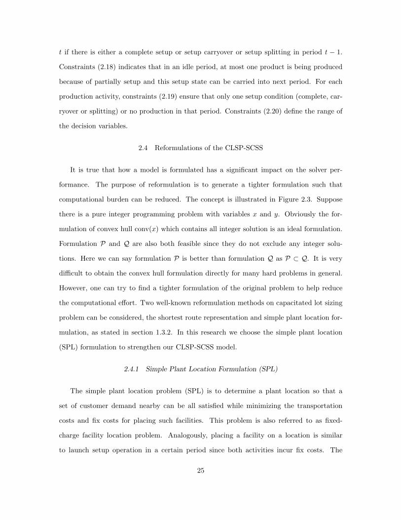
It is true that how a model is formulated has a significant impact on the solver per-

formance. The purpose of reformulation is to generate a tighter formulation such that

computational burden can be reduced. The concept is illustrated in Figure 2.3. Suppose

there is a pure integer programming problem with variables x and y. Obviously the for-

mulation of convex hull conv(x) which contains all integer solution is an ideal formulation.

Formulation P and Q are also both feasible since they do not exclude any integer solu-

tions. Here we can say formulation P is better than formulation Q as P ⊂ Q. It is very

difficult to obtain the convex hull formulation directly for many hard problems in general.

However, one can try to find a tighter formulation of the original problem to help reduce

the computational effort. Two well-known reformulation methods on capacitated lot sizing

problem can be considered, the shortest route representation and simple plant location for-

mulation, as stated in section 1.3.2. In this research we choose the simple plant location

(SPL) formulation to strengthen our CLSP-SCSS model.

2.4.1 Simple Plant Location Formulation (SPL)

The simple plant location problem (SPL) is to determine a plant location so that a

set of customer demand nearby can be all satisfied while minimizing the transportation

costs and fix costs for placing such facilities. This problem is also referred to as fixed-

charge facility location problem. Analogously, placing a facility on a location is similar

to launch setup operation in a certain period since both activities incur fix costs. The

25

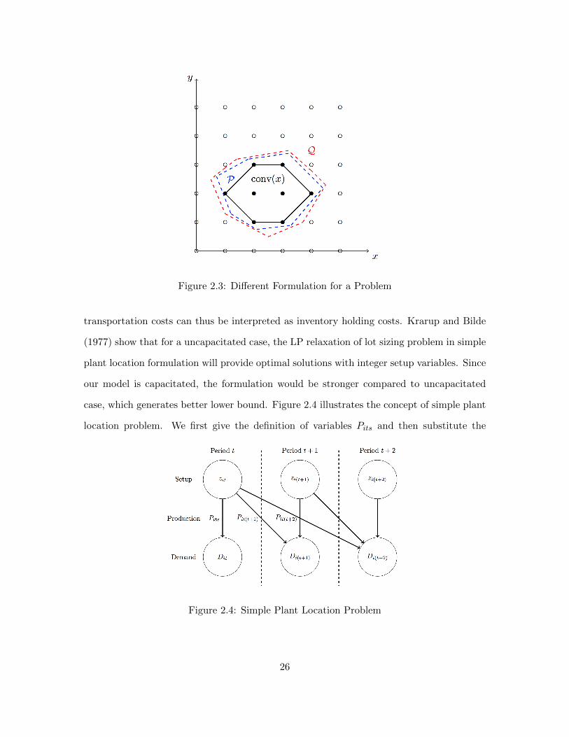
Figure 2.3: Different Formulation for a Problem

transportation costs can thus be interpreted as inventory holding costs. Krarup and Bilde

(1977) show that for a uncapacitated case, the LP relaxation of lot sizing problem in simple

plant location formulation will provide optimal solutions with integer setup variables. Since

our model is capacitated, the formulation would be stronger compared to uncapacitated

case, which generates better lower bound. Figure 2.4 illustrates the concept of simple plant

location problem. We first give the definition of variables Pits and then substitute the

Figure 2.4: Simple Plant Location Problem

26

production quantity variables xit by variables Pits based on equation (2.21). Pits represent

the proportion of demand of product i in period t to satisfy demand in period s, where

s ≥ t.

xit :=T∑s=t

Dis · Pits ∀i, t (2.21)

Since the definition of variable Pits here is to represent the proportion of demand, the range

of variables is bounded in the range [0, 1].

Minimize:N∑i=1

T∑t=1

T∑s=t

hi · (s− t) ·Dit ·Pits +N∑i=1

T∑t=1

SCi · (zit + vit) +T∑t=1

PCt ·Ot (2.22)

Subject to:

zit +Qt ≤ 1 ∀i, t (2.9)

ui(t+1) + uit ≤ 1 +Qt ∀i, t (2.10)

fit + li(t−1) = vit · STt ∀i, t (2.15)

N∑i=1

(uit + vit) ≤ 1 ∀t (2.16)

uit ≤ zi(t−1) + ui(t−1) + vi(t−1) ∀i, t (2.17)

ui(t+1) + vit ≤ 1 +Qt ∀i, t (2.18)

zit + uit + vit ≤ 1 ∀i, t (2.19)

N∑i=1

T∑s=t

Bi ·Dis · Pits +

N∑i=1

(zit · STi + fit + lit) ≤ Ct +Ot ∀t (2.23)

Pits ≤ zit + uit + vit ∀i, t, s = t, ..., T (2.24)

t∑s=1

Pist = 1 ∀i, t provided Dit > 0 (2.25)

Pits, Ot, Qt, fit, lit ≥ 0, ui1 = vi1 = 0, zit, uit, vit ∈ {0, 1} (2.26)

Compared to CLSP-SCSS formulation, there are only several differences. The production

quantity variables xit in the objective function (2.12) and constraints (2.13) are substituted

27

with the proportional variables Pist in (2.22) and (2.23) respectively. Constraints (2.24)

state that production take place only if there is either a complete setup, setup carryover

or setup splitting of product i in period t. Constraints (2.25) must be added to ensure the

range of the proportional variables. All other constraints remain the same from previous

formulation CLSP-SCSS. The SPL formulation of CLSP-SCSS (SPL-SCSS) is consists of

3NT binary variables, at most NT (T+12 ) continuous variables and NT (T+1

2 ) + 7NT + 2T

constraints.

2.4.2 Extended Formulation

Even though the SPL model is a tighter formulation already, we can further extend the

formulation. We here adopted the similar idea presented by Suerie and Stadtler (2003).

They redefine the idle indicator variables Qt by making it become product-dependent vari-

ables QQit.

Variable Definition

QQit QQit = 1 means a product i in period t is produced purely

in an idle period and the setup state is carried into next

period.

Similar to Qt, QQit here does not necessarily to be declared as binary variables (QQi1 =

QQiT = 0). The definition of variable QQit can replace constraints (2.9) in the SPL

formulation with the following:

zit +∑i

QQit ≤ 1 ∀i, t (2.27)

We subtract the right-hand-side by vit + uit −QQit, resulting in (2.28).

zit + uit + vit +∑k 6=i

QQkt ≤ 1 ∀i, t (2.28)

Constraint (2.28) is valid because of the following reasons: a product i in period t can

either have a complete setup (zit = 1) or a carried over from previous period (uit = 1) or a

28

splitting setup (vit = 1), or any other single-item production for any k 6= i in period t (one

QQkt = 1). The possible condition discussed here are obviously mutually exclusive. Next

we can replace constraint (2.17) with (2.29) since the variable QQit indicate for an item i

the setup can be carried over from previous complete setup (zi(t−1) = 1) or the setup has

already carried over from t− 2 to t− 1, which also implies QQi(t−1) = 1.

uit ≤ zi(t−1) +QQi(t−1) ∀i, t = 2, ..., T (2.29)

Constraints (2.10) and (2.18) now can be dropped as they are dominated by (2.28) and

(2.29) now. In addition, we need to add constraints (2.30) and (2.31) to restrict the range

of QQit variables.

QQit ≤ uis + vis ∀i, t = 2, .., T − 1, s = t, ..., t+ 1. (2.30)

QQit ≥ 0 (QQi1 = 0, QQiT = 0) ∀i, t (2.31)

Finally, we included constraints (2.32) for the following reasons. For a product i in period

t, if there is a complete setup in period t− 1, it is unnecessary to perform a setup splitting

for the production of product i in period t.

vit + zi(t−1) ≤ 1 ∀i, t = 2, .., T (2.32)

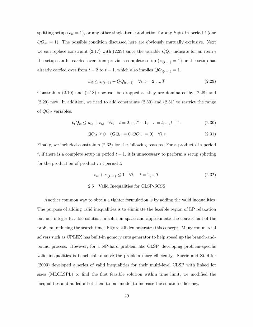
2.5 Valid Inequalities for CLSP-SCSS

Another common way to obtain a tighter formulation is by adding the valid inequalities.

The purpose of adding valid inequalities is to eliminate the feasible region of LP relaxation

but not integer feasible solution in solution space and approximate the convex hull of the

problem, reducing the search time. Figure 2.5 demonstrates this concept. Many commercial

solvers such as CPLEX has built-in gomory cuts generator to help speed up the branch-and-

bound process. However, for a NP-hard problem like CLSP, developing problem-specific

valid inequalities is beneficial to solve the problem more efficiently. Suerie and Stadtler

(2003) developed a series of valid inequalities for their multi-level CLSP with linked lot

sizes (MLCLSPL) to find the first feasible solution within time limit, we modified the

inequalities and added all of them to our model to increase the solution efficiency.

29

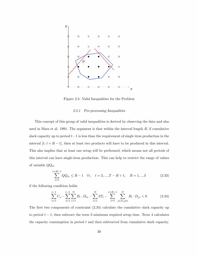
Figure 2.5: Valid Inequalities for the Problem

2.5.1 Pre-processing Inequalities

This concept of this group of valid inequalities is derived by observing the data and also

used in Maes et al. 1991. The argument is that within the interval length R, if cumulative

slack capacity up to period t−1 is less than the requirement of single item production in the

interval [t; t+R− 1], then at least two products will have to be produced in this interval.

This also implies that at least one setup will be performed, which means not all periods of

this interval can have single-item production. This can help to restrict the range of values

of variable QQit.

t+R−1∑s=t

QQis ≤ R− 1 ∀i, t = 2, ..., T −R+ 1, R = 1, .., 3 (2.33)

if the following condition holds:

t−1∑s=1

Cs −t−1∑s=1

N∑i=1

Bi ·Dis −N∑i=1

STi −t+R−1∑s=t

N∑j∈N,j 6=i

Bi ·Djs < 0 (2.34)

The first two components of constraint (2.34) calculate the cumulative slack capacity up

to period t− 1, then subtract the term 3 minimum required setup time. Term 4 calculates

the capacity consumption in period t and then subtracted from cumulative slack capacity.

30

Note that when R = 1, QQit are forced to 0 if slack capacity condition is fulfilled. As the

effect of these constraints disappear gradually when R increases, Suerie and Stadtler (2003)

formulated these constraints for R ≤ 3. Here we adopt the same idea with them for our

extended formulation.

2.5.2 Inventory/Setup Inequalities

If zit = uit = vit = 0 for a product i in period t, there is no production of i in t.

Thus the demand for product i in period t (Dit) must be satisfied from previous inventory

(Ii(t−1)). The same condition holds in interval [t; t+ p] as well, if there is no carryover into

the beginning of interval (uit = 0) and no setup activities throughout the interval (either

zit, ..., zi(t+p) or vit, ..., vi(t+p)=0). This leads to the following valid inequalities:

Ii(t−1) ≥t+p∑s=t

Dis · (1− uit−s∑

r=t

zir −s∑

r=t

vir) ∀i, t = 1, ..., T − 1 p = 1, ..., T − t (2.35)

Constraints (2.35) can be further formulated with the proportional variables Pits in SPL

formulation.

r∑s=t

Pisr ≤ uit +

r∑s=t

zis +

r∑s=t

vis ∀i, r = 1, ..., T t = 1, ..., r (2.36)

2.5.3 Single-item Production Inequalities

The last set of valid inequalities is the combination of capacity balance constraints and

single-item production variables XQit. We first define the new variable XQit.

Variable Definition

XQit single-item production quantity of product i in period t,

where period t is an idle period and setup state is linked

from previous period.

In (2.37), the range of XQit is restricted to production quantity. Constraints (2.38)

reduce XQit to 0 if there is no single-item production (QQit = 0). If there is a single-item

31

production in period t, capacity consumption is restricted to production of XQit, on the

other hand, if there is no single-item production, then constraints (2.39) become just the

capacity constraint of the original CLSP-SCSS model.

XQit ≤ xit ∀i, t = 2, ..., T − 1 (2.37)

XQit ≤ min(Ct

Bi,

T∑s=t

Dis) ·QQit (2.38)

N∑i=1

(xit ·Bi + zit · STi + fit + lit) ≤ Ct · (1−N∑i=1

QQit)

+N∑i=1

XQit ·Bi +Ot ∀t = 2, ..., T − 1 (2.39)

2.6 Inclusion of Backlogging

Another realistic consideration happens often in industrial practice is to allow the pos-

sibility of backlogging in CLSP-SCSS. Basically, the demand now can be met from previous

inventory, current production and later production with additional penalty costs. To ad-

dress this feature, the modification in the basic model and SPL formulation is essential.

Literature regarding to this matter can be found in Wu and Shi (2009, 2011) and Wu et al.

(2013). In this section, we present the inclusion of backlogging to CLSP-SCSS. Furthermore,

we present the strong formulation of including backlogging in the SPL-SCSS.

2.6.1 CLSP-SCSS with Backlogging

First, we introduce the definition of backlogging variables and the associated backlogging

cost. Then replace constraints (2.2) with (2.40) and add constraints (2.41) to make sure no

backlogging unit is allowed in the last period. The corresponding backlogging costs incur

because of allowing backlogging in the production flow. The objective function of CLSP-

SCSS in (2.12) now becomes the new one (2.42). Only these modifications are needed in

the original CLSP-SCSS model.

32

Variable Definition

bgit backlogging unit of product i in period t

BCi backlogging cost for product i

xit + Ii(t−1) + bgit − bgi(t−1) = Dit + Iit ∀i, t (2.40)

bgiT = 0 (2.41)

Minimize:N∑i=1

T∑t=1

SCi · (zit + vit) +N∑i=1

T∑t=1

Hi · Iit

+N∑i=1

T∑t=1

BCi · bgit +T∑t=1

PCt ·Ot (2.42)

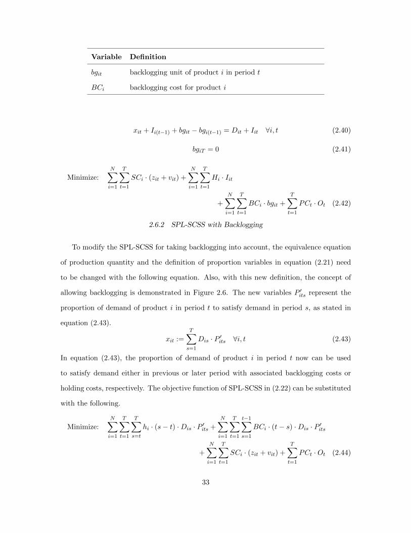
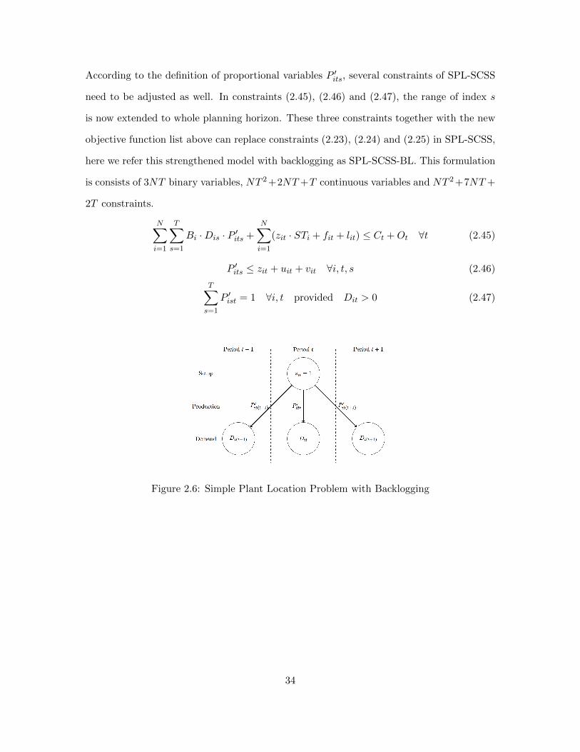
2.6.2 SPL-SCSS with Backlogging

To modify the SPL-SCSS for taking backlogging into account, the equivalence equation

of production quantity and the definition of proportion variables in equation (2.21) need

to be changed with the following equation. Also, with this new definition, the concept of

allowing backlogging is demonstrated in Figure 2.6. The new variables P ′its represent the

proportion of demand of product i in period t to satisfy demand in period s, as stated in

equation (2.43).

xit :=

T∑s=1

Dis · P ′its ∀i, t (2.43)

In equation (2.43), the proportion of demand of product i in period t now can be used

to satisfy demand either in previous or later period with associated backlogging costs or

holding costs, respectively. The objective function of SPL-SCSS in (2.22) can be substituted

with the following.

Minimize:N∑i=1

T∑t=1

T∑s=t

hi · (s− t) ·Dis · P ′its +

N∑i=1

T∑t=1

t−1∑s=1

BCi · (t− s) ·Dis · P ′its

+N∑i=1

T∑t=1

SCi · (zit + vit) +T∑t=1

PCt ·Ot (2.44)

33

According to the definition of proportional variables P ′its, several constraints of SPL-SCSS

need to be adjusted as well. In constraints (2.45), (2.46) and (2.47), the range of index s

is now extended to whole planning horizon. These three constraints together with the new

objective function list above can replace constraints (2.23), (2.24) and (2.25) in SPL-SCSS,

here we refer this strengthened model with backlogging as SPL-SCSS-BL. This formulation

is consists of 3NT binary variables, NT 2+2NT +T continuous variables and NT 2+7NT +

2T constraints.

N∑i=1

T∑s=1

Bi ·Dis · P ′its +

N∑i=1

(zit · STi + fit + lit) ≤ Ct +Ot ∀t (2.45)

P ′its ≤ zit + uit + vit ∀i, t, s (2.46)

T∑s=1

P ′ist = 1 ∀i, t provided Dit > 0 (2.47)

Figure 2.6: Simple Plant Location Problem with Backlogging

34

Chapter 3

SOLUTION APPROACH

The complexity of CLSP with setup time has been shown to be NP-hard, so does the

CLSP-SC and CLSP-SCSS. In mixed integer programming, the number of binary variables

is typically a major indicator of the computational time, that is, the more binary variables,

the more likely the problem would take longer time to solve. In other words, the binary

setup state variables in our model would decelerate the branch-and-bound process. To

obtain the solution in a reasonable amount of time, we applied the fix-and-optimize (F&O)

heuristic to solve the model. First, all the variables of complete setup zit, setup carryover uit

and setup splitting vit are separated into two sets K and L. In each iteration, only a small

subset of zit, uit, vit in L and other decision variables are solved to optimality, while the

rest of binary variables in K are fixed to exogenous value. Two decomposition methods are

used to determine the subproblem: the product decomposition and period decomposition.

Through the iteration guided by the decomposition, the solution is updated when lower costs

are found because of better combination of setup state until no lower costs can be found.

The description of initialization as well as decomposition are discussed in the following

respectively, also a framework of the algorithm is presented.

3.1 Construction of Initial Solution

First we need to select the initial feasible solution for the SPL-SCSS. Typically, there are

many heuristic available to construct the initial feasible solution without spending too much

computational time. For instance, truncated B&B method imposes a time limit for solver

to stop during branch-and-bound process, the incumbent found according to the stopping

criteria can serve as a starting point. The more time allowed the better solution quality can

be found. However, the target of constructive heuristic is not spend too much computational

35

time, truncated B&B might not be a suitable method if the problem size is getting larger

since the time limit would be too short to produce a good solution in terms of optimality

gap, or even no feasible solution can be found. In capacitated lot sizing problem, it is trivial

that having all the complete setups zit = 1 is a feasible schedule to satisfy all the demand.

Nonetheless, this cost is not appealing as the setup carryover does not take effect to remove

unnecessary setups and extra setup costs. In certain cases the period capacity is insufficient

for total setup time, resulting in high penalty costs due to overtime used. Instead of using

this trivial solution at beginning, we solved the LP relaxation of SPL-SCSS and then used

rounding heuristic to round up all the fractional complete setup variables. Given this setup

pattern, we solved the problem again without relaxing the integrality constraints to obtain

corresponding setup pattern for setup carryover and setup splitting. This initialization is

then passing to the algorithm. During the experiment, we examined the solution quality for

several instances and found out that compared to use trivial solution of setting all complete

setups, this initialization gives better solution quality and even true optimal solution can

be found for small size instances. This test result is given in the next chapter.

3.2 Two-stage Decomposition Strategies

We state the major factor of computational time is the number of binary variables at the

beginning of this chapter. The selection of binary variable in set K and L is therefore impor-

tant to the performance of the fix-and-optimize algorithm. Three decomposition strategies

were proposed in Sahling et al. (2009) to treat the multi-level CLSP problem: product

decomposition, period decomposition and process decomposition. They also claimed a

combination of these decomposition strategies is beneficial to obtain high quality solutions.

Here we used the two-stage decomposition methods: first product decomposition then pe-

riod decomposition, as single-level production processes is one of our assumptions. Detail

description for the decomposition methods will be presented in the following.

36

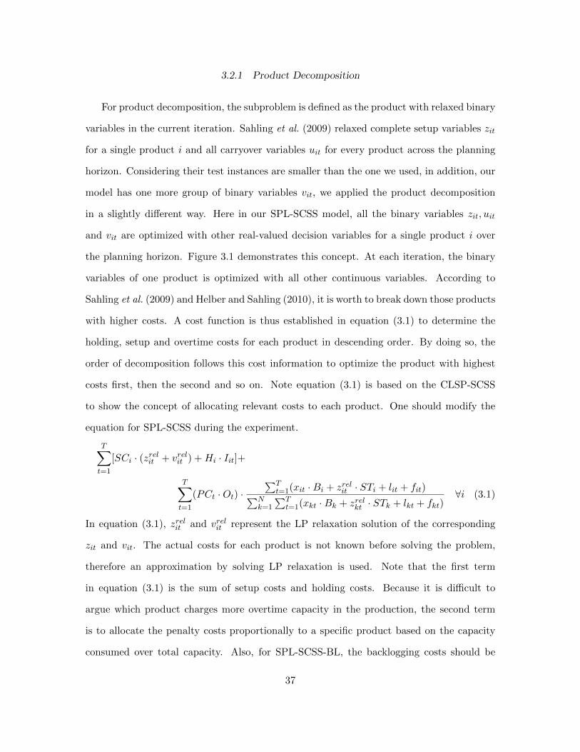
3.2.1 Product Decomposition

For product decomposition, the subproblem is defined as the product with relaxed binary

variables in the current iteration. Sahling et al. (2009) relaxed complete setup variables zit

for a single product i and all carryover variables uit for every product across the planning

horizon. Considering their test instances are smaller than the one we used, in addition, our

model has one more group of binary variables vit, we applied the product decomposition

in a slightly different way. Here in our SPL-SCSS model, all the binary variables zit, uit

and vit are optimized with other real-valued decision variables for a single product i over

the planning horizon. Figure 3.1 demonstrates this concept. At each iteration, the binary

variables of one product is optimized with all other continuous variables. According to

Sahling et al. (2009) and Helber and Sahling (2010), it is worth to break down those products

with higher costs. A cost function is thus established in equation (3.1) to determine the

holding, setup and overtime costs for each product in descending order. By doing so, the

order of decomposition follows this cost information to optimize the product with highest

costs first, then the second and so on. Note equation (3.1) is based on the CLSP-SCSS

to show the concept of allocating relevant costs to each product. One should modify the

equation for SPL-SCSS during the experiment.

T∑t=1

[SCi · (zrelit + vrelit ) +Hi · Iit]+

T∑t=1

(PCt ·Ot) ·∑T

t=1(xit ·Bi + zrelit · STi + lit + fit)∑Nk=1

∑Tt=1(xkt ·Bk + zrelkt · STk + lkt + fkt)

∀i (3.1)

In equation (3.1), zrelit and vrelit represent the LP relaxation solution of the corresponding

zit and vit. The actual costs for each product is not known before solving the problem,

therefore an approximation by solving LP relaxation is used. Note that the first term

in equation (3.1) is the sum of setup costs and holding costs. Because it is difficult to

argue which product charges more overtime capacity in the production, the second term

is to allocate the penalty costs proportionally to a specific product based on the capacity

consumed over total capacity. Also, for SPL-SCSS-BL, the backlogging costs should be

37

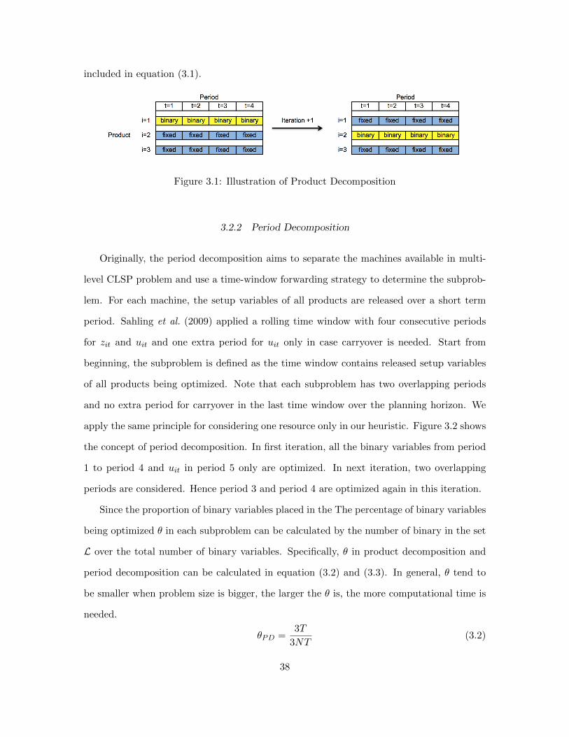
included in equation (3.1).

Figure 3.1: Illustration of Product Decomposition

3.2.2 Period Decomposition

Originally, the period decomposition aims to separate the machines available in multi-

level CLSP problem and use a time-window forwarding strategy to determine the subprob-

lem. For each machine, the setup variables of all products are released over a short term

period. Sahling et al. (2009) applied a rolling time window with four consecutive periods

for zit and uit and one extra period for uit only in case carryover is needed. Start from

beginning, the subproblem is defined as the time window contains released setup variables

of all products being optimized. Note that each subproblem has two overlapping periods

and no extra period for carryover in the last time window over the planning horizon. We

apply the same principle for considering one resource only in our heuristic. Figure 3.2 shows

the concept of period decomposition. In first iteration, all the binary variables from period

1 to period 4 and uit in period 5 only are optimized. In next iteration, two overlapping

periods are considered. Hence period 3 and period 4 are optimized again in this iteration.

Since the proportion of binary variables placed in the The percentage of binary variables

being optimized θ in each subproblem can be calculated by the number of binary in the set

L over the total number of binary variables. Specifically, θ in product decomposition and

period decomposition can be calculated in equation (3.2) and (3.3). In general, θ tend to

be smaller when problem size is bigger, the larger the θ is, the more computational time is

needed.

θPD =3T

3NT(3.2)

38

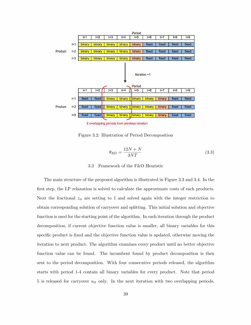
Figure 3.2: Illustration of Period Decomposition

θRD =12N +N

3NT(3.3)

3.3 Framework of the F&O Heuristic

The main structure of the proposed algorithm is illustrated in Figure 3.3 and 3.4. In the

first step, the LP relaxation is solved to calculate the approximate costs of each products.

Next the fractional zit are setting to 1 and solved again with the integer restriction to

obtain corresponding solution of carryover and splitting. This initial solution and objective

function is used for the starting point of the algorithm. In each iteration through the product

decomposition, if current objective function value is smaller, all binary variables for this

specific product is fixed and the objective function value is updated, otherwise moving the

iteration to next product. The algorithm examines every product until no better objective

function value can be found. The incumbent found by product decomposition is then

sent to the period decomposition. With four consecutive periods released, the algorithm

starts with period 1-4 contain all binary variables for every product. Note that period

5 is released for carryover uit only. In the next iteration with two overlapping periods,

39

period 1-2 are now fixed and period 3-6 contain the released binary variables. Similar

to product decomposition, the algorithm goes over the whole planning horizon repeatedly

until no better objective function value can be found. Sahling et al. (2009) and Helber and

Sahling (2010) pointed out one can perform multiple iterations or single iterations in each

decomposition strategies, the algorithm is terminated by setting an external parameter.

In this thesis, we would like to achieve the best performance of the heuristic, hence we

terminate the algorithm until no further improvement can be made.

40

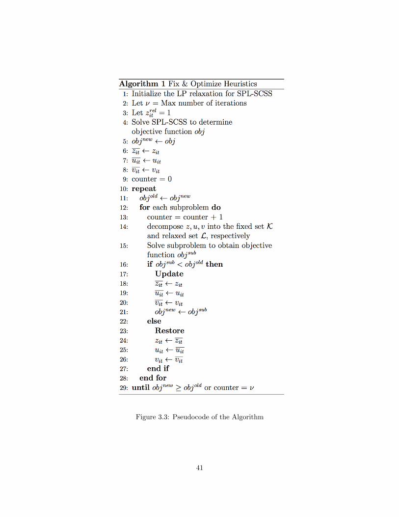
Figure 3.3: Pseudocode of the Algorithm

41

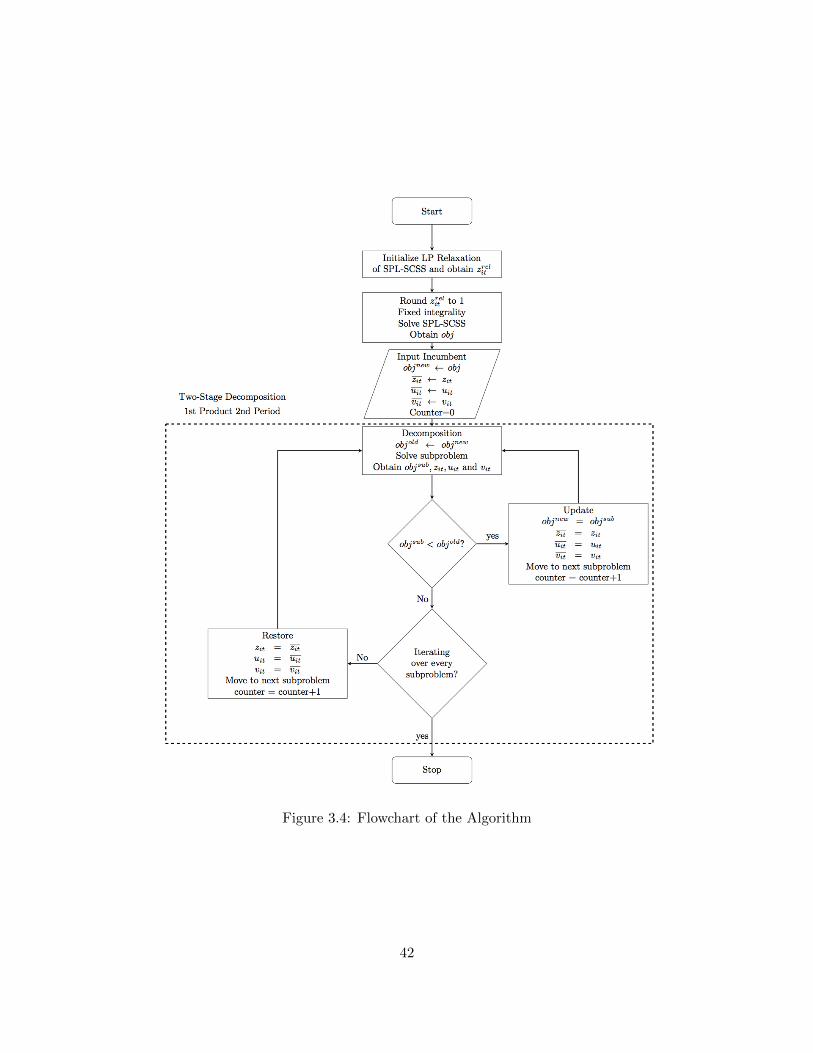
Figure 3.4: Flowchart of the Algorithm

42

Chapter 4

COMPUTATIONAL TEST

In this section, the result of computational test is reported. In addition, the performance

of the algorithm is also analyzed. A Dell Precision T7500 Workstations is used to perform

all the computational test. The processor of the workstation is dual six-core Intel Xeon

Processor X5690 (4.46 GHz, 12M L3, 6.4 GT=s). The memory of the workstation is 48

GB, 1,333 MHz, DDR3RDIMM, ECC (6DIMMS). The proposed extended formulation and

valied inequalities are coded in AMPL and solved by IBM ILOG CPLEX 12.0.6.1.

The fix-and-optimize heuristic is applied on the formulation SPL-SCSS and SPL-SCSS-

BL respectively on the corresponding data. All the valid inequalities are added to SPL-SCSS

in an attempt to enhance the solution efficiency. But the pre-processing valid inequalities

in section 2.5.1 can not be applied to SPL-SCSS-BL since allowing backlogging violates the

condition described in this type of valid inequalities.

In Belo-Filho et al. (2013), a truncated B&B method is used to obtain solution. To be

more precise, they imposed a 600 seconds time limit on the proposed formulation and the

parallel mode was active (4 cores) then used MIP solver to obtain final solution. The result

shows that the proposed formulation CMLM and DSM give best optimality gap for the data

without and with backlogging respectively. The optimality gap is measure by the deviation

of incumbent found from LP relaxation. Since the formulation of CMLM and DSM are

also based on simple plant location, we list the model size of CMLM, DSM, SPL-SCSS and

SPL-SCSS-BL in Table 4.1. Note that their formulation contains one set of variables α to

indicate the model size for long setup time. When α long setup time exist, the number of

constraints in CMLM becomes NT 2 + 7NT + (3α + 2)T , and the number of constraints

in DSM becomes NT 2 + 6NT + (3α + 5)T yet this modification is not necessary in our

standard formulation.

43

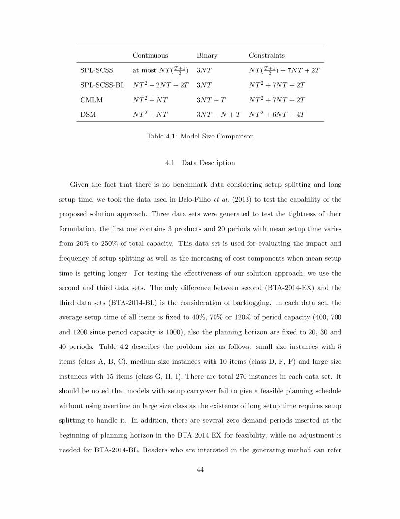
Continuous Binary Constraints

SPL-SCSS at most NT (T+12 ) 3NT NT (T+1

2 ) + 7NT + 2T

SPL-SCSS-BL NT 2 + 2NT + 2T 3NT NT 2 + 7NT + 2T

CMLM NT 2 +NT 3NT + T NT 2 + 7NT + 2T

DSM NT 2 +NT 3NT −N + T NT 2 + 6NT + 4T

Table 4.1: Model Size Comparison

4.1 Data Description

Given the fact that there is no benchmark data considering setup splitting and long

setup time, we took the data used in Belo-Filho et al. (2013) to test the capability of the

proposed solution approach. Three data sets were generated to test the tightness of their

formulation, the first one contains 3 products and 20 periods with mean setup time varies

from 20% to 250% of total capacity. This data set is used for evaluating the impact and

frequency of setup splitting as well as the increasing of cost components when mean setup

time is getting longer. For testing the effectiveness of our solution approach, we use the

second and third data sets. The only difference between second (BTA-2014-EX) and the

third data sets (BTA-2014-BL) is the consideration of backlogging. In each data set, the

average setup time of all items is fixed to 40%, 70% or 120% of period capacity (400, 700

and 1200 since period capacity is 1000), also the planning horizon are fixed to 20, 30 and

40 periods. Table 4.2 describes the problem size as follows: small size instances with 5

items (class A, B, C), medium size instances with 10 items (class D, F, F) and large size

instances with 15 items (class G, H, I). There are total 270 instances in each data set. It

should be noted that models with setup carryover fail to give a feasible planning schedule

without using overtime on large size class as the existence of long setup time requires setup

splitting to handle it. In addition, there are several zero demand periods inserted at the

beginning of planning horizon in the BTA-2014-EX for feasibility, while no adjustment is

needed for BTA-2014-BL. Readers who are interested in the generating method can refer

44

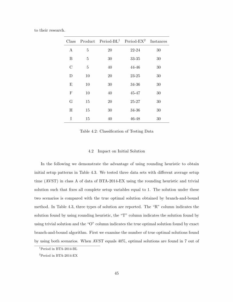
to their research.

Class Product Period-BL1 Period-EX2 Instances

A 5 20 22-24 30

B 5 30 33-35 30

C 5 40 44-46 30

D 10 20 23-25 30

E 10 30 34-36 30

F 10 40 45-47 30

G 15 20 25-27 30

H 15 30 34-36 30

I 15 40 46-48 30

Table 4.2: Classification of Testing Data

4.2 Impact on Initial Solution

In the following we demonstrate the advantage of using rounding heuristic to obtain

initial setup patterns in Table 4.3. We tested three data sets with different average setup

time (AVST) in class A of data of BTA-2014-EX using the rounding heuristic and trivial

solution such that fixes all complete setup variables equal to 1. The solution under these

two scenarios is compared with the true optimal solution obtained by branch-and-bound

method. In Table 4.3, three types of solution are reported. The “R” column indicates the

solution found by using rounding heuristic, the “T” column indicates the solution found by

using trivial solution and the “O” column indicates the true optimal solution found by exact

branch-and-bound algorithm. First we examine the number of true optimal solutions found

by using both scenarios. When AVST equals 40%, optimal solutions are found in 7 out of

1Period in BTA-2014-BL

2Period in BTA-2014-EX

45

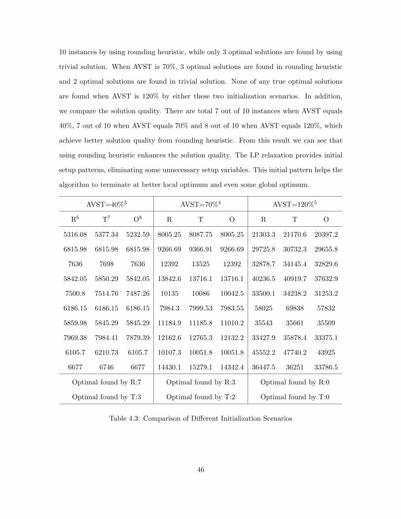
10 instances by using rounding heuristic, while only 3 optimal solutions are found by using

trivial solution. When AVST is 70%, 3 optimal solutions are found in rounding heuristic

and 2 optimal solutions are found in trivial solution. None of any true optimal solutions

are found when AVST is 120% by either these two initialization scenarios. In addition,

we compare the solution quality. There are total 7 out of 10 instances when AVST equals

40%, 7 out of 10 when AVST equals 70% and 8 out of 10 when AVST equals 120%, which

achieve better solution quality from rounding heuristic. From this result we can see that

using rounding heuristic enhances the solution quality. The LP relaxation provides initial

setup patterns, eliminating some unnecessary setup variables. This initial pattern helps the

algorithm to terminate at better local optimum and even some global optimum.

AVST=40%3 AVST=70%4 AVST=120%5

R6 T7 O8 R T O R T O

5316.08 5377.34 5232.59 8005.25 8087.75 8005.25 21303.3 21170.6 20397.2

6815.98 6815.98 6815.98 9266.69 9366.91 9266.69 29725.8 30732.3 29655.8

7636 7698 7636 12392 13525 12392 32878.7 34145.4 32829.6

5842.05 5850.29 5842.05 13842.6 13716.1 13716.1 40236.5 40919.7 37632.9

7500.8 7514.76 7487.26 10135 10086 10042.5 33500.1 34238.2 31253.2

6186.15 6186.15 6186.15 7984.3 7999.53 7983.55 58025 69838 57832

5859.98 5845.29 5845.29 11184.9 11185.8 11010.2 35543 35661 35509

7969.38 7984.41 7879.39 12162.6 12765.3 12132.2 33427.9 35878.4 33375.1

6105.7 6210.73 6105.7 10107.3 10051.8 10051.8 45552.2 47740.2 43925

6677 6746 6677 14430.1 15279.1 14342.4 36447.5 36251 33786.5

Optimal found by R:7 Optimal found by R:3 Optimal found by R:0

Optimal found by T:3 Optimal found by T:2 Optimal found by T:0

Table 4.3: Comparison of Different Initialization Scenarios

46

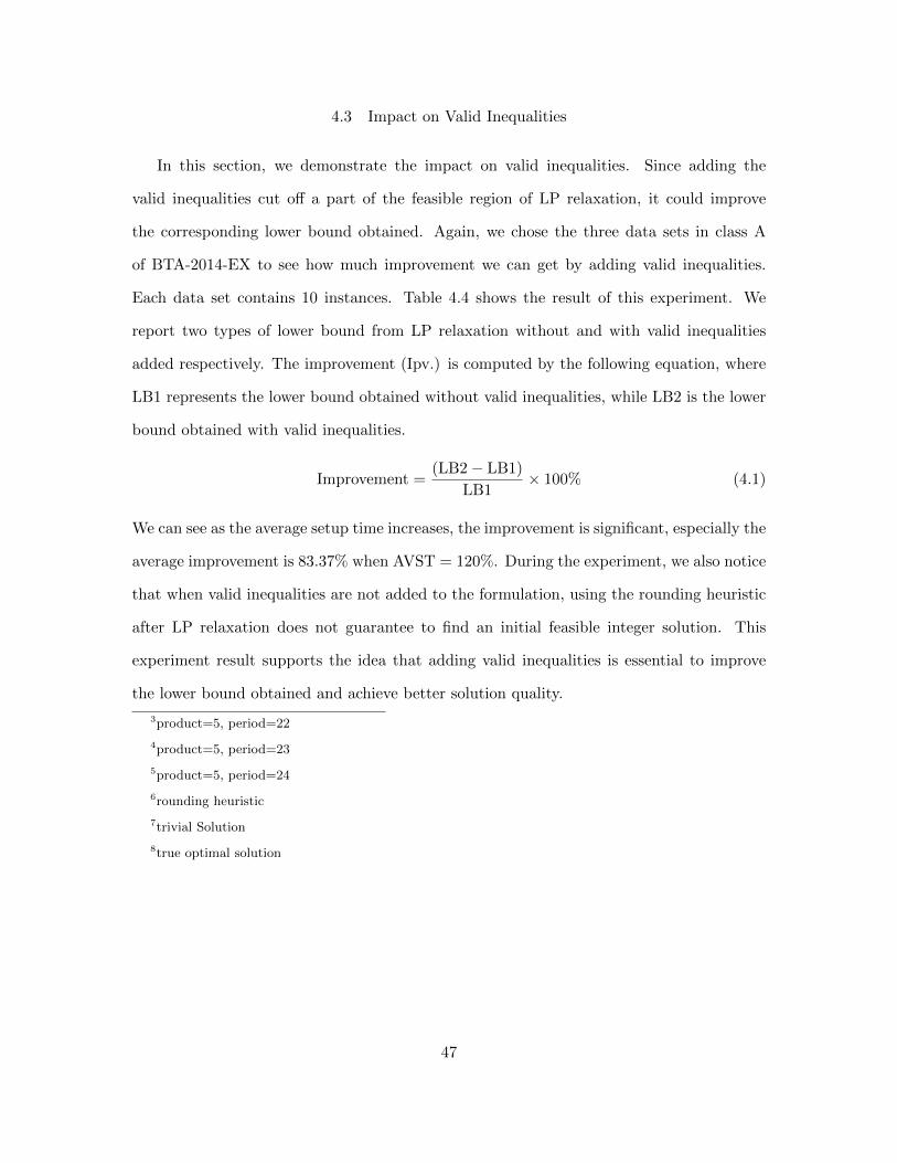
4.3 Impact on Valid Inequalities

In this section, we demonstrate the impact on valid inequalities. Since adding the

valid inequalities cut off a part of the feasible region of LP relaxation, it could improve

the corresponding lower bound obtained. Again, we chose the three data sets in class A

of BTA-2014-EX to see how much improvement we can get by adding valid inequalities.

Each data set contains 10 instances. Table 4.4 shows the result of this experiment. We

report two types of lower bound from LP relaxation without and with valid inequalities

added respectively. The improvement (Ipv.) is computed by the following equation, where

LB1 represents the lower bound obtained without valid inequalities, while LB2 is the lower

bound obtained with valid inequalities.

Improvement =(LB2− LB1)

LB1× 100% (4.1)

We can see as the average setup time increases, the improvement is significant, especially the

average improvement is 83.37% when AVST = 120%. During the experiment, we also notice

that when valid inequalities are not added to the formulation, using the rounding heuristic

after LP relaxation does not guarantee to find an initial feasible integer solution. This

experiment result supports the idea that adding valid inequalities is essential to improve

the lower bound obtained and achieve better solution quality.

3product=5, period=22

4product=5, period=23

5product=5, period=24

6rounding heuristic

7trivial Solution

8true optimal solution

47

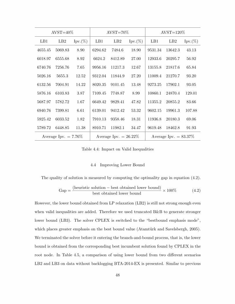
AVST=40% AVST=70% AVST=120%

LB1 LB2 Ipv.(%) LB1 LB2 Ipv.(%) LB1 LB2 Ipv.(%)

4655.45 5069.83 8.90 6294.62 7484.6 18.90 9531.34 13642.3 43.13

6018.97 6555.68 8.92 6624.2 8412.89 27.00 12933.6 20295.7 56.92

6740.76 7256.76 7.65 9956.16 11217.3 12.67 13155.8 21817.6 65.84

5026.16 5655.3 12.52 9312.04 11844.9 27.20 11009.4 21270.7 93.20

6132.56 7004.91 14.22 8020.35 9101.45 13.48 9273.25 17902.1 93.05

5876.16 6103.83 3.87 7109.45 7748.87 8.99 10860.1 24870.4 129.01

5687.97 5782.72 1.67 6649.42 9829.41 47.82 11355.2 20855.2 83.66

6940.76 7399.81 6.61 6139.01 9412.42 53.32 9602.15 19961.3 107.88

5925.42 6033.52 1.82 7910.13 9358.46 18.31 11936.8 20180.3 69.06

5789.72 6448.85 11.38 8910.71 11982.1 34.47 9619.48 18462.8 91.93

Average Ipv. = 7.76% Average Ipv. = 26.22% Average Ipv. = 83.37%

Table 4.4: Impact on Valid Inequalities

4.4 Improving Lower Bound

The quality of solution is measured by computing the optimality gap in equation (4.2).

Gap =(heuristic solution− best obtained lower bound)

best obtained lower bound× 100% (4.2)

However, the lower bound obtained from LP relaxation (LB2) is still not strong enough even

when valid inequalities are added. Therefore we used truncated B&B to generate stronger

lower bound (LB3). The solver CPLEX is switched to the “bestbound emphasis mode”,

which places greater emphasis on the best bound value (Atamturk and Savelsbergh, 2005).

We terminated the solver before it entering the branch-and-bound process, that is, the lower

bound is obtained from the corresponding best incumbent solution found by CPLEX in the

root node. In Table 4.5, a comparison of using lower bound from two different scenarios

LB2 and LB3 on data without backlogging BTA-2014-EX is presented. Similar to previous

48

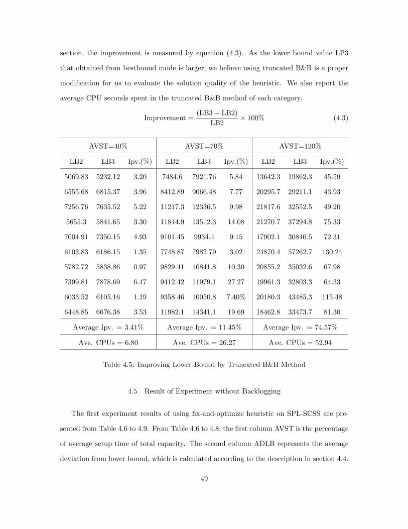
section, the improvement is measured by equation (4.3). As the lower bound value LP3

that obtained from bestbound mode is larger, we believe using truncated B&B is a proper

modification for us to evaluate the solution quality of the heuristic. We also report the

average CPU seconds spent in the truncated B&B method of each category.

Improvement =(LB3− LB2)

LB2× 100% (4.3)

AVST=40% AVST=70% AVST=120%

LB2 LB3 Ipv.(%) LB2 LB3 Ipv.(%) LB2 LB3 Ipv.(%)

5069.83 5232.12 3.20 7484.6 7921.76 5.84 13642.3 19862.3 45.59

6555.68 6815.37 3.96 8412.89 9066.48 7.77 20295.7 29211.1 43.93

7256.76 7635.52 5.22 11217.3 12336.5 9.98 21817.6 32552.5 49.20

5655.3 5841.65 3.30 11844.9 13512.3 14.08 21270.7 37294.8 75.33

7004.91 7350.15 4.93 9101.45 9934.4 9.15 17902.1 30846.5 72.31

6103.83 6186.15 1.35 7748.87 7982.79 3.02 24870.4 57262.7 130.24

5782.72 5838.86 0.97 9829.41 10841.8 10.30 20855.2 35032.6 67.98

7399.81 7878.69 6.47 9412.42 11979.1 27.27 19961.3 32803.3 64.33

6033.52 6105.16 1.19 9358.46 10050.8 7.40% 20180.3 43485.3 115.48

6448.85 6676.38 3.53 11982.1 14341.1 19.69 18462.8 33473.7 81.30

Average Ipv. = 3.41% Average Ipv. = 11.45% Average Ipv. = 74.57%

Ave. CPUs = 6.80 Ave. CPUs = 26.27 Ave. CPUs = 52.94

Table 4.5: Improving Lower Bound by Truncated B&B Method

4.5 Result of Experiment without Backlogging

The first experiment results of using fix-and-optimize heuristic on SPL-SCSS are pre-

sented from Table 4.6 to 4.9. From Table 4.6 to 4.8, the first column AVST is the percentage

of average setup time of total capacity. The second column ADLB represents the average

deviation from lower bound, which is calculated according to the description in section 4.4.

49

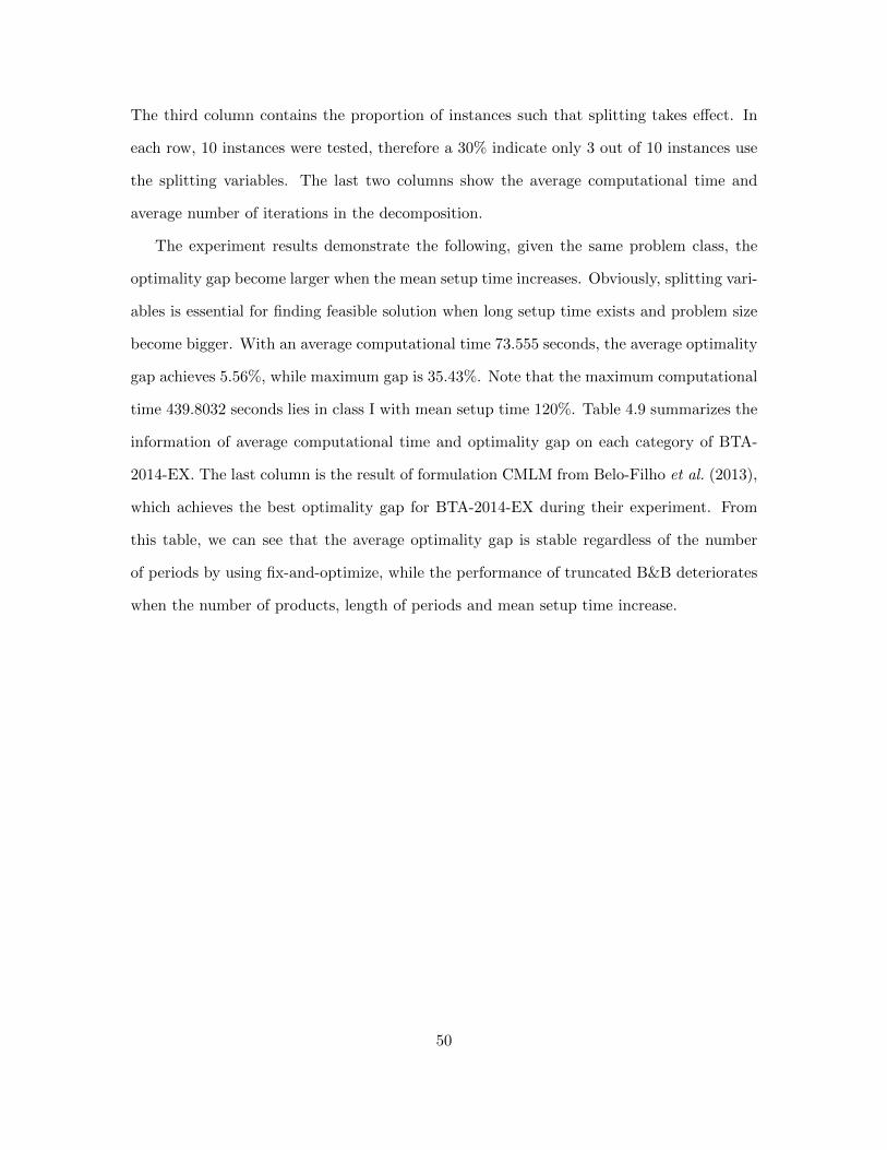
The third column contains the proportion of instances such that splitting takes effect. In

each row, 10 instances were tested, therefore a 30% indicate only 3 out of 10 instances use

the splitting variables. The last two columns show the average computational time and

average number of iterations in the decomposition.

The experiment results demonstrate the following, given the same problem class, the

optimality gap become larger when the mean setup time increases. Obviously, splitting vari-

ables is essential for finding feasible solution when long setup time exists and problem size

become bigger. With an average computational time 73.555 seconds, the average optimality

gap achieves 5.56%, while maximum gap is 35.43%. Note that the maximum computational

time 439.8032 seconds lies in class I with mean setup time 120%. Table 4.9 summarizes the

information of average computational time and optimality gap on each category of BTA-

2014-EX. The last column is the result of formulation CMLM from Belo-Filho et al. (2013),

which achieves the best optimality gap for BTA-2014-EX during their experiment. From

this table, we can see that the average optimality gap is stable regardless of the number

of periods by using fix-and-optimize, while the performance of truncated B&B deteriorates

when the number of products, length of periods and mean setup time increase.

50

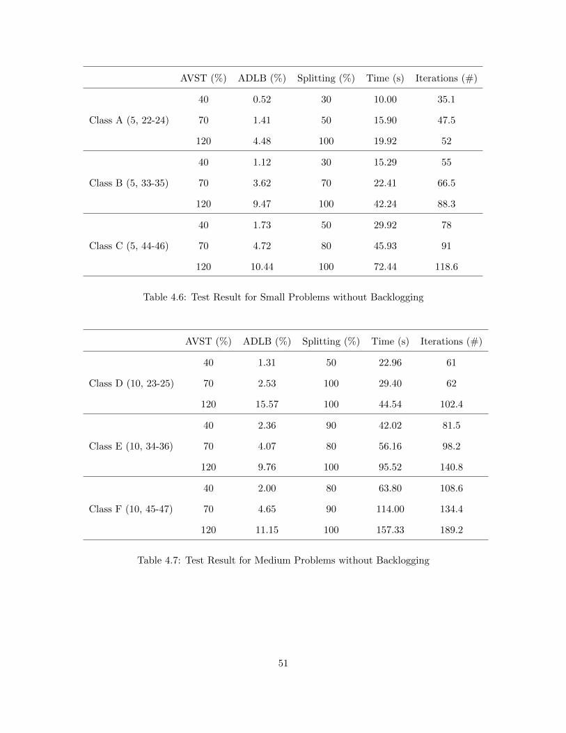
AVST (%) ADLB (%) Splitting (%) Time (s) Iterations (#)

Class A (5, 22-24)

40 0.52 30 10.00 35.1

70 1.41 50 15.90 47.5

120 4.48 100 19.92 52

Class B (5, 33-35)

40 1.12 30 15.29 55

70 3.62 70 22.41 66.5

120 9.47 100 42.24 88.3

Class C (5, 44-46)

40 1.73 50 29.92 78

70 4.72 80 45.93 91

120 10.44 100 72.44 118.6

Table 4.6: Test Result for Small Problems without Backlogging

AVST (%) ADLB (%) Splitting (%) Time (s) Iterations (#)

Class D (10, 23-25)

40 1.31 50 22.96 61

70 2.53 100 29.40 62

120 15.57 100 44.54 102.4

Class E (10, 34-36)

40 2.36 90 42.02 81.5

70 4.07 80 56.16 98.2

120 9.76 100 95.52 140.8

Class F (10, 45-47)

40 2.00 80 63.80 108.6

70 4.65 90 114.00 134.4

120 11.15 100 157.33 189.2

Table 4.7: Test Result for Medium Problems without Backlogging

51

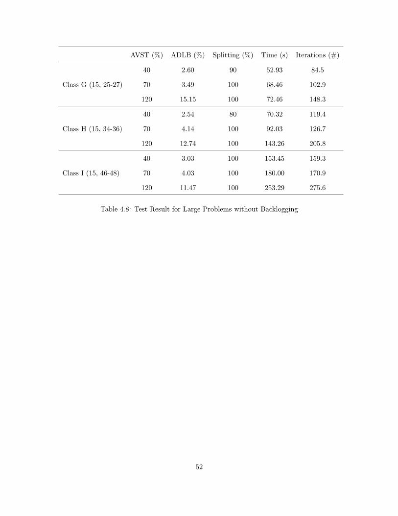
AVST (%) ADLB (%) Splitting (%) Time (s) Iterations (#)

Class G (15, 25-27)

40 2.60 90 52.93 84.5

70 3.49 100 68.46 102.9

120 15.15 100 72.46 148.3

Class H (15, 34-36)

40 2.54 80 70.32 119.4

70 4.14 100 92.03 126.7

120 12.74 100 143.26 205.8

Class I (15, 46-48)

40 3.03 100 153.45 159.3

70 4.03 100 180.00 170.9

120 11.47 100 253.29 275.6

Table 4.8: Test Result for Large Problems without Backlogging

52

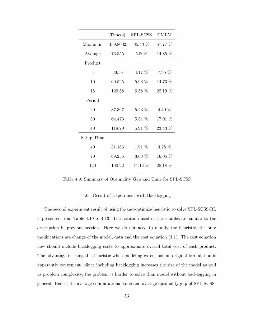
Time(s) SPL-SCSS CMLM

Maximum 439.8032 35.43 % 57.77 %

Average 73.555 5.56% 14.85 %

Product

5 30.56 4.17 % 7.95 %

10 69.525 5.93 % 14.73 %

15 120.58 6.58 % 22.19 %

Period

20 37.397 5.23 % 4.49 %

30 64.473 5.54 % 17.01 %

40 118.79 5.91 % 23.43 %

Setup Time

40 51.186 1.91 % 3.78 %

70 69.255 3.63 % 16.05 %

120 100.22 11.14 % 25.18 %

Table 4.9: Summary of Optimality Gap and Time for SPL-SCSS

4.6 Result of Experiment with Backlogging

The second experiment result of using fix-and-optimize heuristic to solve SPL-SCSS-BL

is presented from Table 4.10 to 4.13. The notation used in these tables are similar to the

description in previous section. Here we do not need to modify the heuristic, the only

modifications are change of the model, data and the cost equation (3.1). The cost equation

now should include backlogging costs to approximate overall total cost of each product.

The advantage of using this heuristic when modeling extensions on original formulation is

apparently convenient. Since including backlogging increases the size of the model as well

as problem complexity, the problem is harder to solve than model without backlogging in

general. Hence, the average computational time and average optimality gap of SPL-SCSS-

53

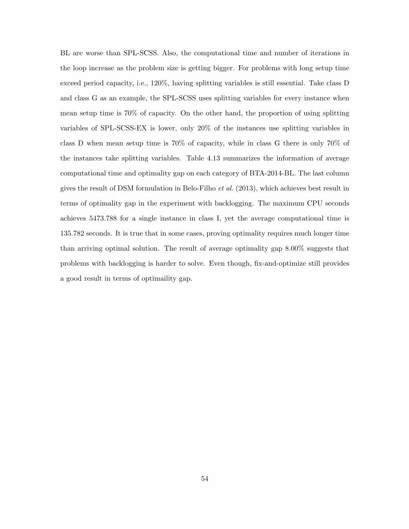
BL are worse than SPL-SCSS. Also, the computational time and number of iterations in

the loop increase as the problem size is getting bigger. For problems with long setup time

exceed period capacity, i.e., 120%, having splitting variables is still essential. Take class D

and class G as an example, the SPL-SCSS uses splitting variables for every instance when

mean setup time is 70% of capacity. On the other hand, the proportion of using splitting

variables of SPL-SCSS-EX is lower, only 20% of the instances use splitting variables in

class D when mean setup time is 70% of capacity, while in class G there is only 70% of

the instances take splitting variables. Table 4.13 summarizes the information of average

computational time and optimality gap on each category of BTA-2014-BL. The last column

gives the result of DSM formulation in Belo-Filho et al. (2013), which achieves best result in

terms of optimality gap in the experiment with backlogging. The maximum CPU seconds

achieves 5473.788 for a single instance in class I, yet the average computational time is

135.782 seconds. It is true that in some cases, proving optimality requires much longer time

than arriving optimal solution. The result of average optimality gap 8.00% suggests that

problems with backlogging is harder to solve. Even though, fix-and-optimize still provides

a good result in terms of optimaility gap.

54

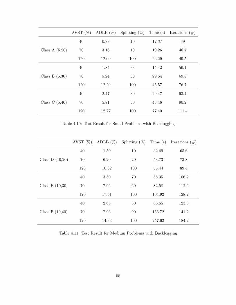
AVST (%) ADLB (%) Splitting (%) Time (s) Iterations (#)

Class A (5,20)

40 0.88 10 12.37 39

70 3.16 10 19.26 46.7

120 12.00 100 22.29 49.5

Class B (5,30)

40 1.84 0 15.42 56.1

70 5.24 30 29.54 69.8

120 12.20 100 45.57 76.7

Class C (5,40)

40 2.47 30 29.47 93.4

70 5.81 50 43.46 90.2

120 12.77 100 77.40 111.4

Table 4.10: Test Result for Small Problems with Backlogging

AVST (%) ADLB (%) Splitting (%) Time (s) Iterations (#)

Class D (10,20)

40 1.50 10 32.49 65.6

70 6.20 20 53.73 73.8

120 10.32 100 55.44 89.4

Class E (10,30)

40 3.50 70 58.35 106.2

70 7.96 60 82.58 112.6

120 17.51 100 104.92 128.2

Class F (10,40)

40 2.65 30 86.65 123.8

70 7.96 90 155.72 141.2

120 14.33 100 257.62 184.2

Table 4.11: Test Result for Medium Problems with Backlogging

55

AVST (%) ADLB (%) Splitting (%) Time (s) Iterations (#)

Class G (15,20)

40 4.74 50 69.55 107.1

70 13.92 70 110.36 119.6

120 12.24 100 135.54 122.7

Class H (15,30)

40 3.25 70 110.19 134.8

70 11.01 60 194.90 147.5

120 12.30 100 270.91 169.9

Class I (15,40)

40 3.60 80 243.04 165.9

70 10.55 70 321.11 187.5

120 6.03 100 1029.21 217.5

Table 4.12: Test Result for Large Problems with Backlogging

56

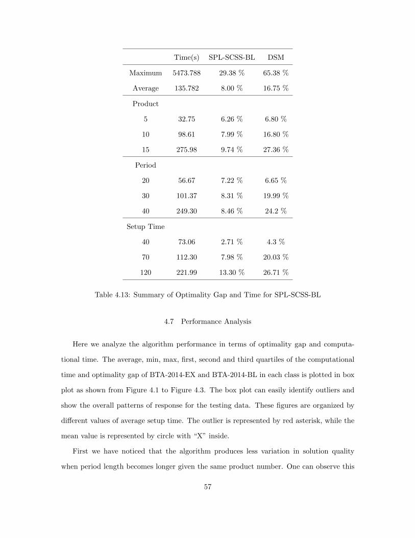
Time(s) SPL-SCSS-BL DSM

Maximum 5473.788 29.38 % 65.38 %

Average 135.782 8.00 % 16.75 %

Product

5 32.75 6.26 % 6.80 %

10 98.61 7.99 % 16.80 %

15 275.98 9.74 % 27.36 %

Period

20 56.67 7.22 % 6.65 %

30 101.37 8.31 % 19.99 %

40 249.30 8.46 % 24.2 %

Setup Time

40 73.06 2.71 % 4.3 %

70 112.30 7.98 % 20.03 %

120 221.99 13.30 % 26.71 %

Table 4.13: Summary of Optimality Gap and Time for SPL-SCSS-BL

4.7 Performance Analysis

Here we analyze the algorithm performance in terms of optimality gap and computa-

tional time. The average, min, max, first, second and third quartiles of the computational

time and optimality gap of BTA-2014-EX and BTA-2014-BL in each class is plotted in box

plot as shown from Figure 4.1 to Figure 4.3. The box plot can easily identify outliers and

show the overall patterns of response for the testing data. These figures are organized by

different values of average setup time. The outlier is represented by red asterisk, while the

mean value is represented by circle with “X” inside.

First we have noticed that the algorithm produces less variation in solution quality

when period length becomes longer given the same product number. One can observe this

57

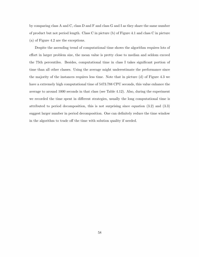
by comparing class A and C, class D and F and class G and I as they share the same number

of product but not period length. Class C in picture (b) of Figure 4.1 and class C in picture

(a) of Figure 4.2 are the exceptions.

Despite the ascending trend of computational time shows the algorithm requires lots of

effort in larger problem size, the mean value is pretty close to median and seldom exceed

the 75th percentiles. Besides, computational time in class I takes significant portion of

time than all other classes. Using the average might underestimate the performance since

the majority of the instances requires less time. Note that in picture (d) of Figure 4.3 we

have a extremely high computational time of 5473.788 CPU seconds, this value enhance the

average to around 1000 seconds in that class (see Table 4.12). Also, during the experiment

we recorded the time spent in different strategies, usually the long computational time is

attributed to period decomposition, this is not surprising since equation (3.2) and (3.3)

suggest larger number in period decomposition. One can definitely reduce the time window

in the algorithm to trade off the time with solution quality if needed.

58

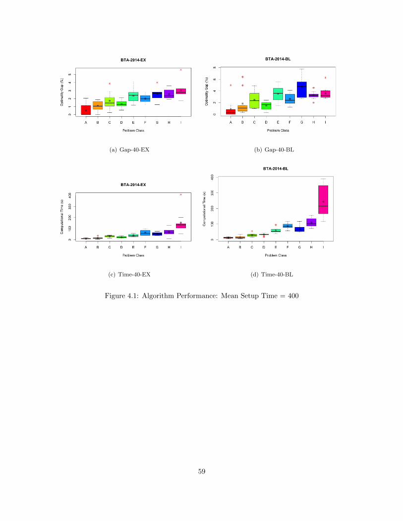
(a) Gap-40-EX (b) Gap-40-BL

(c) Time-40-EX (d) Time-40-BL

Figure 4.1: Algorithm Performance: Mean Setup Time = 400

59

(a) Gap-70-EX (b) Gap-70-BL

(c) Time-70-EX (d) Time-70-BL

Figure 4.2: Algorithm Performance: Mean Setup Time = 700

60

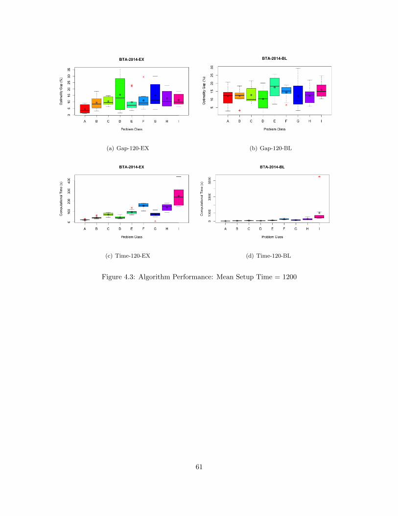
(a) Gap-120-EX (b) Gap-120-BL

(c) Time-120-EX (d) Time-120-BL

Figure 4.3: Algorithm Performance: Mean Setup Time = 1200

61

Chapter 5

CONCLUSION AND FUTURE DIRECTIONS

In this thesis, we study the single level, single machine, multi-item capacitated lot sizing

problem with setup carryover, setup splitting and backlogging. To our best knowledge, there

has been no such research for lot sizing problems consider setup carryover, setup splitting

and backlogging together yet. This thesis aims to fill in this gap.

In chapter 2, we present the formulations of the basic capacitated lot sizing problem

and extend it with setup carryover, setup splitting, simple plant location formulation and

backlogging consideration. Three sets of valid inequalities from literature are developed and

discussed.

In chapter 3, we describe the structure of fix-and-optimize heuristic, including the con-

struction of initial solution by using rounding heuristic and then demonstrate that for some

small size problems, using rounding heuristic instead of trivial solution can guarantee to

find the true optimal solution. A two-stage decomposition strategies: product and period

decomposition are presented. In order to justify how good the solution can be found by

this approach, we do not limit the number of iterations and computational time in the

algorithm. Instead, the algorithm terminates until no further improvement can be found in

each subproblem.

Chapter 4 includes several computational experiments. First, we demonstrate the benefit

on using rounding heuristic by showing how many true optimal solution can be found. Then

the impact on lower bound of adding valid inequalities is given. Lower bound is further

improved by using truncated B&B method. The next two sections summarize the result

of the two computational tests on experiments without and with backlogging. From the

analysis, the performance of algorithm tends to be stable in terms of average optimality gap

regardless of the number of periods when backlogging is not allowed. Such property can be

62

beneficial for company to extend the planning horizon, which is more common and practical

in reality than increasing product types. In addition, less variations of the solution quality

are observed in larger problem size given the same product numbers.

Modeling setup features in lot sizing problem usually done by binary variables. Adopting

fix-and-optimize heuristic to solve the problem gives advantage as the heuristic mainly

decomposes binary variables, resulting in smaller subproblems. We also demonstrate the

effectiveness of combining other mathematical programming based approaches including

rounding heuristic, reformulation as well as valid inequalities. Another advantage of fix-and-

optimize heuristic would be the easiness to implement and flexibility when other features are

included in the model, such as backlogging in our case. Other approaches such as Lagrangian

relaxation heuristic, which is usually considered very problem-specific, requiring redesign of

the whole process when extra constraints are added and does not necessarily produce an

easy subproblem after relaxing the hard constraints. To sum up, a comprehensive evaluation

with more instances and other potential algorithms would be beneficial.

Several possibilities could be examined in future research. For instance, considering

other MIP-based heuristic, metaheuristic or even a hybrid approach to justify the solution

quality and computational time on different algorithms. Developing specific valid inequali-

ties for lot sizing problems with setup splitting and backlogging to improve the lower bound

from LP relaxation. In addition, other model extension such as multi-level, parallel machine

or sequence-dependent setup time and setup costs can be considered in the next step.

63

REFERENCES

Akartunalı, K. and A. J. Miller, “A heuristic approach for big bucket multi-level productionplanning problems”, European Journal of Operational Research 193, 2, 396–411 (2009).

Atamturk, A. and M. W. Savelsbergh, “Integer-programming software systems”, Annals ofOperations Research 140, 1, 67–124 (2005).

Barany, I., T. J. Van Roy and L. A. Wolsey, “Strong formulations for multi-item capacitatedlot sizing”, Management Science 30, 10, 1255–1261 (1984).

Belo-Filho, M. A., F. M. Toledo and B. Almada-Lobo, “Models for capacitated lot-sizingproblem with backlogging, setup carryover and crossover”, Journal of the OperationalResearch Society 65, 11, 1735–1747 (2013).

Belvaux, G. and L. A. Wolsey, “bc—prod: A specialized branch-and-cut system for lot-sizing problems”, Management Science 46, 5, 724–738 (2000).

Belvaux, G. and L. A. Wolsey, “Modelling practical lot-sizing problems as mixed-integerprograms”, Management Science 47, 7, 993–1007 (2001).

Bitran, G. R. and H. H. Yanasse, “Computational complexity of the capacitated lot sizeproblem”, Management Science 28, 10, 1174–1186 (1982).

Buschkuhl, L., F. Sahling, S. Helber and H. Tempelmeier, “Dynamic capacitated lot-sizingproblems: a classification and review of solution approaches”, OR Spectrum 32, 2, 231–261 (2010).

Denizel, M., F. T. Altekin, H. Sural and H. Stadtler, “Equivalence of the lp relaxationsof two strong formulations for the capacitated lot-sizing problem with setup times”, ORspectrum 30, 4, 773–785 (2008).

Dıaz-Madronero, M., J. Mula and D. Peidro, “A review of discrete-time optimization modelsfor tactical production planning”, International Journal of Production Research 52, 17,5171–5205 (2014).

Dillenberger, C., L. F. Escudero, A. Wollensak and W. Zhang, “On solving a large-scale re-source allocation problem in production planning”, in “Operations research in productionplanning and control”, pp. 105–119 (Springer, 1993).

Drexl, A. and K. Haase, “Proportional lotsizing and scheduling”, International Journal ofProduction Economics 40, 1, 73–87 (1995).

Drexl, A. and A. Kimms, “Lot sizing and scheduling—survey and extensions”, EuropeanJournal of Operational Research 99, 2, 221–235 (1997).

Eppen, G. D. and R. K. Martin, “Solving multi-item capacitated lot-sizing problems usingvariable redefinition”, Operations Research 35, 6, 832–848 (1987).

Federgruen, A., J. Meissner and M. Tzur, “Progressive interval heuristics for multi-itemcapacitated lot-sizing problems”, Operations Research 55, 3, 490–502 (2007).

Fiorotto, D. J., R. Jans and S. A. de Araujo, “An analysis of formulations for the capacitatedlot sizing problem with setup crossover”, (2014).

64

Florian, M., J. K. Lenstra and A. Rinnooy Kan, “Deterministic production planning: Al-gorithms and complexity”, Management science 26, 7, 669–679 (1980).

Gicquel, C., M. Minoux and Y. Dallery, “Capacitated lot sizing models: a literature review”,(2008).

Gopalakrishnan, M., “A modified framework for modelling set-up carryover in the capaci-tated lotsizing problem”, International Journal of Production Research 38, 14, 3421–3424(2000).

Gopalakrishnan, M., K. Ding, J.-M. Bourjolly and S. Mohan, “A tabu-search heuristic forthe capacitated lot-sizing problem with set-up carryover”, Management Science 47, 6,851–863 (2001).

Gopalakrishnan, M., D. Miller and C. Schmidt, “A framework for modelling setup carryoverin the capacitated lot sizing problem”, International Journal of Production Research 33,7, 1973–1988 (1995).

Goren, H. G., S. Tunali and R. Jans, “A hybrid approach for the capacitated lot sizingproblem with setup carryover”, International Journal of Production Research 50, 6, 1582–1597 (2012).

Gupta, D. and T. Magnusson, “The capacitated lot-sizing and scheduling problem withsequence-dependent setup costs and setup times”, Computers & Operations Research32, 4, 727–747 (2005).

Haase, K., Lotsizing and scheduling for production planning (Springer, Berlin, 1994).

Haase, K., Capacitated lot-sizing with linked production quantities of adjacent periods(Springer, 1998).

Harris, F. W., “How many parts to make at once”, Operations Research 38, 6, 947–950(1990).

Helber, S. and F. Sahling, “A fix-and-optimize approach for the multi-level capacitated lotsizing problem”, International Journal of Production Economics 123, 2, 247–256 (2010).

Hsu, W.-L., “On the general feasibility test of scheduling lot sizes for several products onone machine”, Management Science 29, 1, 93–105 (1983).

Jans, R. and Z. Degraeve, “Meta-heuristics for dynamic lot sizing: A review and comparisonof solution approaches”, European Journal of Operational Research 177, 3, 1855–1875(2007).

Karimi, B., S. F. Ghomi and J. Wilson, “The capacitated lot sizing problem: a review ofmodels and algorithms”, Omega 31, 5, 365–378 (2003).

Kopanos, G. M., L. Puigjaner and C. T. Maravelias, “Production planning and scheduling ofparallel continuous processes with product families”, Industrial & engineering chemistryresearch 50, 3, 1369–1378 (2011).

Krarup, J. and O. Bilde, Plant Location, Set Covering and Economic Lot Size: An 0 (mn)-Algorithm for Structured Problems (Springer, 1977).

65

Lang, J. C. and Z.-J. M. Shen, “Fix-and-optimize heuristics for capacitated lot-sizing withsequence-dependent setups and substitutions”, European Journal of Operational Research214, 3, 595–605 (2011).

Maes, J., J. O. McClain and L. N. Van Wassenhove, “Multilevel capacitated lotsizing com-plexity and lp-based heuristics”, European Journal of Operational Research 53, 2, 131–148 (1991).

Menezes, A. A., A. Clark and B. Almada-Lobo, “Capacitated lot-sizing and scheduling withsequence-dependent, period-overlapping and non-triangular setups”, Journal of Schedul-ing 14, 2, 209–219 (2011).

Miller, A. J., G. L. Nemhauser, M. W. Savelsbergh et al., Solving multi-item capacitated lot-sizing problems with setup times by branch-and-cut (Universite Catholique de Louvain.Center for Operations Research and Econometrics [CORE], 2000).

Mohan, S., M. Gopalakrishnan, R. Marathe and A. Rajan, “A note on modelling the ca-pacitated lot-sizing problem with set-up carryover and set-up splitting”, InternationalJournal of Production Research 50, 19, 5538–5543 (2012).

Pochet, Y. and L. A. Wolsey, “Solving multi-item lot-sizing problems using strong cuttingplanes”, Management Science 37, 1, 53–67 (1991).

Pochet, Y. and L. A. Wolsey, Production planning by mixed integer programming (SpringerScience & Business Media, 2006).

Quadt, D. and H. Kuhn, “Capacitated lot-sizing with extensions: a review”, 4OR 6, 1,61–83 (2008).

Quadt, D. and H. Kuhn, “Capacitated lot-sizing and scheduling with parallel machines,back-orders, and setup carry-over”, Naval Research Logistics (NRL) 56, 4, 366–384(2009).

Rogers, J., “A computational approach to the economic lot scheduling problem”, Manage-ment Science 4, 3, 264–291 (1958).

Rosling, K., “Optimal lot-sizing for dynamic assembly systems”, in “Multi-stage productionplanning and inventory control”, pp. 119–131 (Springer, 1986).

Sahling, F., L. Buschkuhl, H. Tempelmeier and S. Helber, “Solving a multi-level capacitatedlot sizing problem with multi-period setup carry-over via a fix-and-optimize heuristic”,Computers & Operations Research 36, 9, 2546–2553 (2009).

Sox, C. R. and Y. Gao, “The capacitated lot sizing problem with setup carry-over”, IIetransactions 31, 2, 173–181 (1999).

Stadtler, H., “Mixed integer programming model formulations for dynamic multi-item multi-level capacitated lotsizing”, European Journal of Operational Research 94, 3, 561–581(1996).

Stadtler, H., “Reformulations of the shortest route model for dynamic multi-item multi-levelcapacitated lotsizing”, OR Spectrum 19, 2, 87–96 (1997).

Stadtler, H., “Multilevel lot sizing with setup times and multiple constrained resources:Internally rolling schedules with lot-sizing windows”, Operations Research 51, 3, 487–502 (2003).

66

Suerie, C., “Modeling of period overlapping setup times”, European Journal of OperationalResearch 174, 2, 874–886 (2006).

Suerie, C. and H. Stadtler, “The capacitated lot-sizing problem with linked lot sizes”,Management Science 49, 8, 1039–1054 (2003).

Sung, C. and C. T. Maravelias, “A mixed-integer programming formulation for the gen-eral capacitated lot-sizing problem”, Computers & Chemical Engineering 32, 1, 244–259(2008).

Tempelmeier, H. and S. Helber, “A heuristic for dynamic multi-item multi-level capacitatedlotsizing for general product structures”, European Journal of Operational Research 75,2, 296–311 (1994).

Trigeiro, W. W., L. J. Thomas and J. O. McClain, “Capacitated lot sizing with setuptimes”, Management Science 35, 3, 353–366 (1989).

Wagner, H. M. and T. M. Whitin, “Dynamic version of the economic lot size model”,Management science 5, 1, 89–96 (1958).

Wu, T., K. Akartunalı, J. Song and L. Shi, “Mixed integer programming in productionplanning with backlogging and setup carryover: modeling and algorithms”, Discrete EventDynamic Systems 23, 2, 211–239 (2013).

Wu, T. and L. Shi, “A new heuristic method for capacitated multi-level lot sizing problemwith backlogging”, in “Automation Science and Engineering, 2009. CASE 2009. IEEEInternational Conference on”, pp. 483–488 (IEEE, 2009).

Wu, T. and L. Shi, “Mathematical models for capacitated multi-level production planningproblems with linked lot sizes”, International Journal of Production Research 49, 20,6227–6247 (2011).

Xiao, J., C. Zhang, L. Zheng and J. N. Gupta, “Mip-based fix-and-optimise algorithmsfor the parallel machine capacitated lot-sizing and scheduling problem”, InternationalJournal of Production Research 51, 16, 5011–5028 (2013).

67

APPENDIX A

ACRONYMS

68

Notation Description

B&B Branch-and-bound

CLSP Capacitated Lot Sizing Problem

CLSP-SC Capacitated Lot Sizing Problem with Setup Carryover

CLSPL Capacitated Lot Sizing Problem with Linked Lot Sizes

CLSP-SCSS Capacitated Lot Sizing Problem with Setup Carryover and Setup Split-

ting

CLSD Capacitated Lot Sizing Problem with Sequence-dependent Setup Time

and Setup Costs

CLSD-S Capacitated Lot Sizing Problem with Sequence-dependent Setup Time

and Substitutions

CSLP Continuous Lot Sizing Problem

DLSP Discrete Lot Sizing Problem

EOQ Economical Ordering Quantity

F&O Fix-and-optimize Heuristic

MIP Mixed Integer Programming

MRP Material Requirement Planning

MRP II Manufacturing Resource Planning

MLCLSP Multi-level Capacitated Lot Sizing Problem

MLCLSPL Multi-level Capacitated Lot Sizing Problem with Linked Lot Sizes

PLSP Proportional Lot Sizing Problem

RH Rounding Heuristic

R&F Relax-and-fix Heuristic

SR Shortest Route

SPL Simple Plant Location

SPL-SCSS SPL formulation for CLSP-SCSS

SPL-SCSS-BL SPL formulation for CLSP-SCSS with Demand Backlogging

69