a novel solution approach to capacitated lot-sizing problems with setup times and setup carry-over

ABSTRACT

KARAGUL, HAKAN FATIH. A Novel Solution Approach to Capacitated Lot-Sizing

Problems with Setup Times and Setup Carry-Over. (Under the direction of Donald P.

Warsing and Thom J. Hodgson.)

In this study we propose a novel mixed integer linear programming (MILP)

formulation to solve capacitated lot-sizing problems (CLSP) with setup times and setup carry

over. We compare our novel formulation to two formulations in the literature by solving

single- and multiple-machine instances with and without holding costs. We refer to one of

these original formulations as the ―classical formulation,‖ and we call the other, which is

modified from the classical formulation, the ―modified formulation.‖ Extensive

computational tests show that our novel formulation consistently outperforms both the

classical formulation and the modified formulation in terms of the computation time required

to achieve an optimal or near-optimal solution and the resulting solution gap, which measures

the difference between the best upper bound and the best lower bound in the branch and

bound tree used to solve these mixed-integer-programming formulations. Our experiments

also show that the modified formulation is superior to the classical formulation in terms of

gap and computation time performance. We demonstrate that the main difference between

the classical formulation and the modified formulation comes from the structure of their

respective branch and bound trees. We also demonstrate that the LP relaxation of our novel

formulation provides a tighter lower bound as compared to the modified formulation. For

problems in which production lots must be allocated across 2m parallel machines, the

branch and bound solution process unfortunately results in larger upper bound-lower bound

gaps, but the novel formulation continues to perform better than the classical and modified

formulations. The solution to a relaxed, single-machine formulation of the parallel-machine

problem that is based on our novel formulation, however, leads to a substantially tighter

lower bound than those generated by the branch and bound solutions, and we use this to

demonstrate that our time-restricted MIP solutions are actually quite good in terms of the

upper bound (incumbent solution). This relaxed formulation also leads directly to a heuristic

approach that can solve the parallel-machine problem in less than one minute, on average.

This heuristic solves the problems in our experiments to within 1.4% of the single-machine

formulation bound, on average, although the heuristic solution for some instances reflects a

gap of 5% or higher.

A Novel Solution Approach to Capacitated Lot-Sizing Problems

with Setup Times and Setup Carry-Over

by

Hakan Fatih Karagul

A dissertation submitted to the Graduate Faculty of

North Carolina State University

in partial fulfillment of the

requirements for the Degree of

Doctor of Philosophy

Industrial Engineering

Raleigh, North Carolina

2012

APPROVED BY:

_______________________________ ______________________________

Thom J. Hodgson Donald P. Warsing

Committee Co-Chair Committee Co-Chair

________________________________ ________________________________

Reha Uzsoy Russell E. King

ii

DEDICATION

This thesis is dedicated to

My Mother, Ayfer

My Father, Hasan

My Brother, Huseyin Iskender

and

My beautiful fiancée Sibel

iii

BIOGRAPHY

Hakan Fatih Karagul was born on June 24th

, 1984 in Istanbul, Turkey. After

graduating from German High School in Istanbul he attended Istanbul Technical University

and received his Bachelor degree in Mechanical Engineering. Upon graduation he started

working at Mercedes-Benz Turkey and served as a supply chain engineer in the logistics

department. In 2008, he joined the Department of Industrial and Systems Engineering at

North Carolina State University. After completing the degree requirements for the Masters

degree he began pursuing his Ph.D. degree in Industrial Engineering. During his time at

North Carolina State University his research was funded by Xerox Corporation and he

worked as a researcher at Xerox Corporation in the summers of 2009 and 2010. He also

served as a Research and Teaching assistant at North Carolina State University. In January

2010, he was elected Vice President of the University Graduate Student Association (UGSA)

and served as Vice President of External Affairs. Upon receiving his PhD degree, Hakan will

join Enova Financial in Chicago, IL as an Advanced Analytics Associate.

iv

ACKNOWLEDGMENTS

This dissertation would not have been possible without the invaluable guidance and

support of my advisors Dr. Donald Warsing, Dr. Thom J. Hodgson, Dr. Reha Uzsoy and Dr.

Russell E. King. I am thankful that they believed in me and gave me the chance to work on

this project.

I would like to thank Dr. Sudhendu Rai and Kenneth Mihalyov from Xerox

Corporation for their generous support. I am grateful to them for the invaluable feedback

they provided during this research.

I would also like to thank my friends Dr. Erinc Albey, Dr. Yasin Alan and Dr. Ali

Kefeli for their collaboration, input and support. I thank my friends Nils Buch, Kuang-Hao

Buch, Peter Prim, Sean Carr, Krishna Jarugumilli, Emine Yaylali, Dr. Jennifer Mason, Dr.

Benjamin Lobo, Dr. Jeremy Tejada, Dr. Bjorn Berg and Dr. Baris Kacar for providing a great

atmosphere in the Department of Industrial and Systems Engineering at NC State University.

Last, but not least, I would like to thank my family Hasan Karagul, Ayfer Karagul,

Dr. Huseyin Iskender Karagul and my beautiful fiancée Sibel Oktay for their endless support,

patience, love and understanding.

v

Table of Contents

LIST OF TABLES .................................................................................................................. vii

LIST OF FIGURES ................................................................................................................. ix

1 INTRODUCTION ............................................................................................................ 1

1.1 Literature Review ....................................................................................................... 3

1.1.1 Lot-Sizing Literature ........................................................................................... 3

1.1.2 Scheduling Literature .......................................................................................... 5

1.2 Problem Overview...................................................................................................... 7

1.3 Problem Notation and Properties ............................................................................. 11

2 SINGLE-MACHINE FORMULATIONS WITHOUT HOLDING COST .................... 14

2.1 Classical Restricted Capacitated Lot-Sizing Problem (CRCLSP) ........................... 16

2.2 Modified Restricted CLSP (Capacitated Lot-Sizing Problem) ................................ 17

2.3 Novel Formulation ................................................................................................... 22

2.4 Computational Experiments ..................................................................................... 28

2.4.1 Experiment with the Uniform Processing Times .............................................. 29

2.4.2 Experiment with the Mixed Processing Times ................................................. 37

2.5 Comparison of the Formulations .............................................................................. 44

2.5.1 Classical Formulation vs. Modified Formulation ............................................. 44

2.5.2 Modified Formulation vs. Novel Formulation .................................................. 47

2.6 Conclusions .............................................................................................................. 50

3 SINGLE-MACHINE FORMULATIONS WITH HOLDING COST ............................ 53

3.1 Extending the Novel Formulation ............................................................................ 54

3.2 Computational Experiment Results .......................................................................... 55

3.3 Conclusions .............................................................................................................. 60

4 PARALLEL-MACHINE FORMULATIONS ................................................................ 62

4.1 Classical Restricted Capacitated Lot-Sizing Problem with Parallel Machines ........ 64

4.2 Modified Restricted Capacitated Lot-Sizing Problem with Parallel Machines ....... 66

4.3 Novel Formulation with Parallel Machines ............................................................. 67

4.4 Computational Experiments ..................................................................................... 70

4.4.1 Two-Machine Experiment with Uniform Processing Times ............................ 70

4.4.2 Three-Machine Experiment with Uniform Processing Times .......................... 76

vi

4.4.3 Two-Machine Experiment with Holding Cost (Trigeiro Test Bed) .................. 80

4.5 Alternative Lower Bound ......................................................................................... 86

4.6 Heuristic Approach .................................................................................................. 90

4.6.1 Heuristic Algorithm .......................................................................................... 91

4.6.2 Computational Experiments.............................................................................. 95

4.7 Conclusion .............................................................................................................. 110

5 CONCLUSION AND FUTURE WORK ..................................................................... 112

5.1 Summary of Findings ............................................................................................. 112

5.2 Future Work ........................................................................................................... 114

REFERENCES ..................................................................................................................... 117

APPENDICES ...................................................................................................................... 119

Appendix A ........................................................................................................................... 120

Appendix B ........................................................................................................................... 129

Appendix C ........................................................................................................................... 135

vii

LIST OF TABLES

Table 1 - Sample Problem Characteristics .............................................................................. 29

Table 2 - Test Bed Statistics (Slackness) ................................................................................ 31

Table 3 - Test Bed Statistics (Density) ................................................................................... 31

Table 4 - Computation Time Summary, Single Machine, Uniform Processing Times .......... 32

Table 5 - Gap Summary, Single Machine, Uniform Processing Times .................................. 35

Table 6 - Computation Time Summary, Single Machine, Mixed Processing Times ............. 39

Table 7 - Gap Summary, Single Machine, Mixed Processing Times ..................................... 40

Table 8 - Number of Variables (No holding cost) .................................................................. 51

Table 9 - Computation Time Summary, Single Machine, Trigeiro Test bed ......................... 56

Table 10 - Gap Summary, Single Machine, Trigeiro Test bed ............................................... 57

Table 11 - Number of Variables (with holding cost) .............................................................. 60

Table 12 - Computation Time Summary, Two Machines, Uniform Processing Times ......... 71

Table 13 - Gap Summary, Two Machines, Uniform Processing Times ................................. 72

Table 14 - Computation Time Summary, Three Machines, Uniform Processing Times ....... 77

Table 15 - Gap Summary, Three Machines, Uniform Processing Times ............................... 77

Table 16 - Computation Time Summary, Two Machines, Trigeiro Test Bed ........................ 81

Table 17 - Gap Summary, Two Machines, Trigeiro Test Bed ................................................ 82

Table 18 - Example Candidate List ........................................................................................ 92

Table 19 - Gap Summary of the Heuristic, Two Machines, Uniform Distribution ................ 96

Table 20 - Computation Time Summary of the Heuristic, Two Machines, Uniform

Distribution ............................................................................................................................. 97

Table 21 - Gap Summary of the Heuristic, Three Machines, Uniform Distribution ............ 104

viii

Table 22 - Computation Time Summary of the Heuristic, Three Machines, Uniform

Distribution ........................................................................................................................... 104

Table 23 - Simple Linear Transformations ........................................................................... 122

ix

LIST OF FIGURES

Figure 1 - Scheduling Literature Map ....................................................................................... 9

Figure 2 - Lot-Sizing Literature Map...................................................................................... 10

Figure 3 - Classical Formulation............................................................................................. 19

Figure 4 - Modified Formulation ............................................................................................ 19

Figure 5 – Left-Shift ............................................................................................................... 24

Figure 6 – Optimal Solution ................................................................................................... 24

Figure 7 - Fixed Charge Network Flow Interpretation of Novel Formulation ....................... 27

Figure 8 - Average Computation Times vs. Problem size, Single Machine, Uniform

Distribution ............................................................................................................................. 33

Figure 9 - Computation Time Performance, Single Machine, Uniform Distribution

(Cumulative) ........................................................................................................................... 34

Figure 10 - Gap Performance, Single Machine, Uniform Distribution (Cumulative) ............ 36

Figure 11 - Gap Distribution, Single Machine, Uniform Processing Times .......................... 36

Figure 12 - Average Computation Times vs. Problem size, Single Machine, Mixture

Distribution ............................................................................................................................. 40

Figure 13 - Computation Time Performance, Single Machine, Mixture Distribution

(Cumulative) ........................................................................................................................... 42

Figure 14 - Gap Performance, Single Machine, Mixture Distribution (Cumulative) ............. 42

Figure 15 - Gap Distribution, Single Machine, Mixture Distribution .................................... 43

Figure 16 - Branch & Bound Tree of the Classical Formulation ............................................ 46

Figure 17 - Branch & Bound Tree of the Modified Formulation ........................................... 46

Figure 18 - Computation Time Performance, Single Machine, Trigeiro Test Bed

(Cumulative) ........................................................................................................................... 56

Figure 19 - Gap Performance, Single Machine, Trigeiro Test Bed (Cumulative) .................. 58

x

Figure 20 - Gap Distribution, Single Machine, Trigeiro Test Bed ......................................... 59

Figure 21 – Novel Formulation with Parallel Machines ......................................................... 68

Figure 22 - Average Computation Times vs. Problem size, Two Machines, Uniform

Distribution ............................................................................................................................. 73

Figure 23 - Computation Time Performance, Two Machines, Uniform Distribution

(Cumulative) ........................................................................................................................... 74

Figure 24 - Gap Performance, Two Machines, Uniform Distribution (Cumulative) ............. 74

Figure 25 - Gap Distribution, Two-Machine Experiment, Uniform Processing Times ......... 76

Figure 26 - Computation Time Performance, Three Machines, Uniform Distribution

(Cumulative) ........................................................................................................................... 78

Figure 27 - Gap Performance, Three Machines, Uniform Distribution (Cumulative) ........... 79

Figure 28 - Gap Distribution, Three-Machine Experiment, Uniform Processing Times ....... 80

Figure 29 - Computation Time Performance, Two Machines, Trigeiro Experiment

(Cumulative) ........................................................................................................................... 83

Figure 30 - Gap Performance, Two Machines, Trigeiro Experiment (Cumulative) ............... 84

Figure 31 - Gap Distribution, Two Machines, Trigeiro Experiment ...................................... 85

Figure 32 - Gap Performance, Two Machines, Uniform Distribution (Cumulative) ............. 89

Figure 33 - Gap Performance, Three Machines, Uniform Distribution (Cumulative) ........... 89

Figure 34 – Flowchart of the Heuristic ................................................................................... 94

Figure 35 - % Deviation from zSM vs. Density, Two Machines, Uniform Distribution ......... 98

Figure 36 - % Deviation from zSM vs. Slackness, Two Machines, Uniform Distribution ...... 99

Figure 37 – Average Computation Time vs. Density, Two Machines, Uniform Distribution

............................................................................................................................................... 100

Figure 38 – Average Computation Time vs. Slackness, Two Machines, Uniform Distribution

............................................................................................................................................... 100

Figure 39 - Gap Performance, Two Machines, Uniform Distribution (Cumulative) ........... 102

xi

Figure 40 - Distribution of the Deviations, Two Machines, Uniform Distribution .............. 102

Figure 41 - % Deviation from zSM vs. Density, Three Machines, Uniform Distribution ..... 105

Figure 42 - % Deviation from zSM vs. Slackness, Three Machines, Uniform Distribution .. 105

Figure 43 – Average Computation Time vs. Density, Three Machines, Uniform Distribution

............................................................................................................................................... 106

Figure 44 - Average Computation Time vs. Slackness, Three Machines, Uniform Distribution

............................................................................................................................................... 107

Figure 45 – Gap Performance, Three Machines, Uniform Distribution (Cumulative) ......... 108

Figure 46 - Distribution of the Deviations, Three Machines, Uniform Distribution ............ 108

Figure 47 - Lot-for-lot before ―left-shift‖ ............................................................................. 130

Figure 48 - Example of a single "left-shift" .......................................................................... 131

Figure 49 – Optimal Solution ............................................................................................... 131

Figure 50 - Average Computation Time vs. Problem Size, Single Machine, Uniform

Distribution ........................................................................................................................... 133

Figure 51 - Gap Performance, Single Machine, Uniform Distribution (Cumulative) .......... 134


(Cumulative) ......................................................................................................................... 134

Figure 53 - Gap vs. Density and Slackness, Classical Formulation, Two Machines, Uniform

Distribution, p=140 ............................................................................................................... 135

Figure 54 - Gap vs. Density and Slackness, Modified Formulation, Two Machines, Uniform

Distribution, p=140 ............................................................................................................... 136

Figure 55 - Gap vs. Density and Slackness, Novel Formulation, Two Machines, Uniform

Distribution, p=140 ............................................................................................................... 136

Figure 56 - Gap vs. Density and Slackness, Classical Formulation, Three Machines, Uniform

Distribution, p=140 ............................................................................................................... 137

Figure 57 - Gap vs. Density and Slackness, Modified Formulation, Three Machines, Uniform

Distribution, p=140 ............................................................................................................... 137

xii

Figure 58 - Gap vs. Density and Slackness, Novel Formulation, Three Machines, Uniform

Distribution, p=140 ............................................................................................................... 138

1

CHAPTER 1

1 INTRODUCTION

Production planning problems can be categorized into three areas: High-level,

medium-level and low-level planning problems. In high-level production planning activities,

decisions are made regarding total production capacity and/or resource levels to support

production, while medium-level activities mostly deal with production lot-sizing decisions.

By solving lot-sizing problems, planners determine how much to produce and in which

period to produce. Low-level production problems are known as scheduling or sequencing

problems, where the complete sequence of the jobs is determined for different periods in a

production horizon.

Lot-sizing is one of the major issues of production planning and has been studied

extensively in the literature. When production capacity is limited the problem is called a

capacitated lot-sizing problem (CLSP). In this study, we develop a novel formulation to solve

2

capacitated lot-sizing problems for an arbitrary number of periods and an arbitrary number of

production orders (jobs) on both a single machine and across multiple, identical machines

running in parallel. We first formulate our motivating problem, a transactional print-shop

problem, as a special case of the CLSP and then extend our formulation to solve general

CLSP.

The transactional print-shop problem that serves as the motivating problem for this

research concerns a production environment in which customers place orders in ―groups‖ (or

families) whose component jobs may have multiple deadlines. For example, a customer may

order 100 units of product (i.e., 100 printed copies), but request that 50 units be delivered in

three days, 30 units the day after that, and 20 units the day after that. This demand structure

is typical of transactional printing services—e.g., in the printing of various periodic

statements like cable television billing statements or health insurance ―EOBs‖ (―explanation

of benefits‖ forms). This multiple-deadline ordering structure quite likely stems from the

fact that the producer (print shop) and its customers both recognize that the totality of each

customer’s order, or perhaps the orders of just a few customers, would likely consume all of

the producer’s capacity in the short term. Therefore, the customers are willing to alter their

ordering behavior to reflect the fact that each order can be delivered in ―chunks‖ that spread

the consumption of customer capacity in a way that is more manageable for the producer.

Transactional print shops are, moreover, interesting ―flow shop‖ environments, with a

relatively small number of possible routings among various processing tasks (e.g., printing,

cutting, folding and inserting—i.e., into envelopes), but with each being done at a high

3

volume, and with some setup time possibly required at each operation to switch from one job

group (customer order, job family, or product) to the next.

Since this problem can be interpreted as either a scheduling problem or as a lot-

sizing problem, we provide an overview of both bodies of literature in the next section,

followed by the problem overview.

1.1 Literature Review

In this section we look at two strands of literature by first reviewing the lot-sizing

literature and then the scheduling literature.

1.1.1 Lot-Sizing Literature

In production systems, lot-sizing decisions are being made continually and have a

direct impact on operating costs. If planning horizons are long and inventory holding costs

are high, lot-sizing decisions may be critical to reducing inventory costs. Lot-sizing decisions

can also be critical to minimizing non-value-added processes like setups. Being able to

achieve this goal is important if the cost of resources (machines) and the cost of setups are

high. Indeed, print shops are a good example of such an environment. Since industrial

printers are relatively expensive machines, they should process jobs continuously in order to

meet the return-on-investment goals of the company. Moreover, compared to the printing

process, setting up the machine is a laborious process, and therefore it is desirable to

minimize setups.

The classical capacitated lot-sizing problem (CLSP) is a well-known problem that has

been investigated extensively. For instance, Trigeiro et al. [11], Billington et al. [12] and

4

Ritzman and Bahl [13] presented classical capacitated lot-sizing formulations. Bitran and

Yanasse [14] proved that CLSP is NP-Hard even if setup times are not taken into account.

Maes [15] worked on the feasibility problem and demonstrated that this problem is NP-

Complete.

It should be noted that none of these studies above considers ―setup carry-overs‖, also

referred to as ―linked lot-sizes‖. A setup is carried over to the next period when the last job of

a period and the first job of the following period are from the same family and no setup is

required at the beginning of the latter period. Sox and Gao [16] introduced the CLSP

formulation with setup carry-overs. Throughout this study we refer to their formulation as the

classic formulation. According to Haase [17], including setup carry-overs in the problem

formulation changes the optimal solutions significantly. He also showed that restricting setup

carry-overs to only the subsequent period improves the computation time required to solve

the instances, and thus facilitates the solution of bigger problems. However, in that study he

only considered setup costs and ignored setup times. In this dissertation we extend Haase’s

formulation in [17] by including setup times in the capacity constraint. Throughout this study

we refer to his formulation as the modified formulation. Dillenberger [18], on the other hand,

solved real world CLSP problems allowing setup carry-overs and considering setup times by

using a partial branch-and-bound method, but he made the assumption that the production of

a product occurs only in its demand period. Gopalakrishnan [19] proposed a formulation

considering setup carry-overs and setup times, where he presented a computational test with

only two job families and twelve periods. We refer interested readers to the extensive

literature reviews in Quadt et al. [20] and Karimi et al. [21]. There are also studies by Potts et

5

al. [22] and Meyr [23], who reviewed scheduling and lot-sizing decisions for big-bucket and

small-bucket problems. A lot-sizing problem is called a small-bucket problem if its solution

determines the complete sequence of the jobs; otherwise it is called a big-bucket problem.

CLSP falls into the big-bucket category since it doesn’t determine the complete sequence of

jobs.

1.1.2 Scheduling Literature

In the last two decades many researchers have investigated single-machine scheduling

problems involving setup times. If some jobs from the same group (or family) can be

combined into a single batch to eliminate setup times, then the literature calls the problem a

batch setup problem; otherwise, the problem is called a non-batch setup problem [1]. Two

main types of batch-setup problems are defined in the literature: ―batch-availability

formulations‖ and ―job-availability formulations.‖

In batch-availability formulations it is assumed that a job in a batch becomes

available when processing of all jobs in that particular batch is completed. In job-availability

formulations the completion time of each job in a particular batch is independent from other

jobs in the same batch [2]. In this study we focus on batch setup problems with job

availability. Another important issue is setup time characteristics. Setup times might depend

on the sequence of jobs or they can be independent of such a sequence. We assume that setup

times are sequence-independent.

The literature suggests that minimizing maximum lateness is one of the most common

measures of performance in batch setup problems. Moreover, it has been shown by

6

computational experiments that this measure of performance generates ―high quality‖

schedules under certain conditions [3]. Since most of these problems are NP-Hard [4],

heuristic solutions are suggested in many cases. Baker [5] demonstrated that earliest-due-date

sequencing yields the optimum solution if setup times are negligible, and a group technology

approach (jobs from same family are grouped in a single batch) works well if setup times are

relatively long and/or if the due dates are identical. Baker [5] also developed a gap heuristic

and a neighborhood search approach for performance improvement. Uzsoy and Velásquez

[6] improved existing heuristics for this problem and analyzed their performance. In this

study, we focus on problems with no late job constraints, meaning that if a job is not

completed before its deadline, then the schedule is infeasible. In this case minimizing

maximum lateness leads to many optimal solutions which can potentially be improved

further in terms of the total setup cost.

In the motivating context for this research (transactional print shops), inventory

holding costs are not significant compared to setup costs. In addition, setup costs and setup

times are the same for all jobs on each machine. Under these assumptions, objectives such as

minimizing the total setup time, maximizing the setup savings, minimizing the make-span,

minimizing the total number of setups or minimizing the maximum completion time yield

similar results. In this group of objectives the main goal is to batch as many jobs as possible.

In the second chapter of this dissertation, our main concern is minimizing the total setup cost.

In the third chapter we extend our objective function by including holding costs.

As shown by Bruno et al. [7], if deadlines (no tardy jobs allowed) are involved then

the problem is NP-Hard. If there are no due-date restrictions, however, then the group

7

technology approach will give the optimum solution. Unal and Kiran [8] developed an exact

algorithm to find a feasible schedule for the feasibility problem formulated by Bruno et al.

[7]. Driscoll et al. [9] suggested a dynamic programming approach to minimize the total

changeover cost. However, that study assumes that setup times are negligible. It should be

noted that dynamic programming approaches proposed in these papers can be used to solve

small problems, but they are not practical for relatively large problems. For instance Monma

and Potts [10] showed that the computational complexity of their dynamic programming

algorithm is exponential in the number of job families.

In this study we present a novel mixed-integer-programming (MIP) formulation to

solve capacitated lot-sizing problems with setup carry-overs. This novel formulation is a

fixed charge network flow interpretation of the problem. We show that our novel formulation

outperforms the formulations in the literature.

1.2 Problem Overview

We formulate a single-machine, capacitated lot-sizing problem (CLSP) with setup

times and setup carry over. Because we assume that inventory holding cost is zero due to the

short planning horizon and low product cost compared to the setup costs, the problem can

also be described as a single-machine, product family scheduling problem with batching and

deadlines (no late jobs allowed). In this problem, both the setup times and costs are constant,

and therefore sequence-independent. All jobs are available for production at the beginning of

the horizon and a product becomes available for shipment at its completion time, so the

availability of a product does not depend on other jobs in the same batch (item availability).

8

There are T periods in the horizon. In our case these periods are considered to be

weekdays. This is reasonable because in many industries, including the printing industry (the

original motivation for this work), deadlines are defined by days and not by, say, hours. Each

order can have up to T jobs with different deadlines. A job can be due only at the end of a

period. In other words if we have T periods, we have only T different deadlines defined in

our problem. If the deadline of a job is period t, then the job must be completed by the end of

period t. Based on our experience, this ordering structure is not uncommon, especially in

print shops. We refer to each order as a ―family,‖ and no setup is required between jobs from

the same family. If the next job is not from the same family as the current job, then a setup is

required. As mentioned above we also consider setup carry-overs between periods. We

assume that a setup cannot start in one period and complete in the next period. Before

generating the schedule, orders are clustered first. If there are two jobs from the same family

due in the same period, we batch them and consider them as a single job because having two

setups in a single period for jobs from the same family does not serve our objective. Another

assumption we make in this study is that there is no machine breakdown. This means at all

points in time the machine (or the machines) is available for set-up or processing jobs.

Figure 1 shows where our problem formulation (shown in circle) fits in the

scheduling literature.

9

Figure 1 - Scheduling Literature Map

We know that if the number of product families is large, the chance of producing only

a single type of product in an entire period decreases in the optimal solution. If one knows

that production of a single type of product in an entire period is unlikely, then he/she can

restrict the setup carry-overs in the formulation. By restricting the carry-overs we mean that a

setup can be carried over to the next adjacent period but no further. In [17], Haase names the

formulation with such a restriction ―Capacitated Lot-Sizing Formulation with Linked Lot-

Sizes of Adjacent Periods‖.

Scheduling Problems

Single Machine

Without Setups With Setups

Batch

Sequence Dependent

Setups

Sequence Independent

Setups

Minimize Total Flow Time

Minimize Maximum Lateness

Minimize Setup Cost

Others

Non-Batch

Multiple Machine

10

Haase shows that this restriction improves the performance of the formulation

significantly. Transactional print-shops receive hundreds of orders daily and based on our

experience, in transactional print-shops more than one type of job gets processed in each

period (defined as ―day‖ or ―shift‖), so this assumption is reasonable. In other words, in the

single-machine formulation we assume that the processing time of a single job is always less

than the period capacity. Throughout this study, when we say ―performance‖ we mean the

computation time and the gap between the upper and lower bounds from the branch-and-

bound tree, as reported by CPLEX (v. 12.2).

Figure 2 presents where our problem formulation (shown in bold) fits in the lot-sizing

literature.

Figure 2 - Lot-Sizing Literature Map

Capacitated Lot-Sizing Problems

Big Bucket

Without Setup Times

With Setup Times

Without Setup Carry-Over

With Setup Carry-Over

Small Bucket

11

1.3 Problem Notation and Properties

In order to define some important properties of the problem we consider in this

research, we first formally define the parameters that are relevant to the problems studied.

P : Number of job families (products), {1,..., }P P

T : Number of periods, {1,..., }T T

1 if job is due in period

0 otherwisetp

p ty

u

pt : Process time per unit of product p

s

pt : Setup time of product p

ptd : Demand volume of product p in period t

tC : Capacity (i.e. total time available) in period t

An important property of these problems is what we define as the density, , given

by

tp

t T p P

y

TP

, [0 1]

(1)

Density is a measure of the extent to which the ―jobs matrix‖ is filled. If every job

family (or product) has a job due in each period, then the total number of jobs is equal to TP,

12

which is the maximum number of jobs possible. In that case 1 . If there are no jobs at all

then is equal to 0. In other words, based on its definition, 0 1 .

Another important property of these problems is the slackness, t , given by

1

u s

p pt p pt

p P

t

t

t d t y

C

(2)

Since our procedures attempt to save setup time by moving jobs from later periods

into earlier periods, the slackness defined in (2) is a measure of the minimum proportion of

time available in period t into which jobs could be moved. We note, however, that this

measure of slackness underestimates time available since it assumes the maximum number of

setups required to complete the schedule. It should be also noted that t can have negative

values. We use slackness and density parameters later in generating problem instances for

our computational tests.

The dissertation is structured as follows: In Chapter 2 we first present the classical

single-machine, mixed-integer-programming (MIP) formulation found in the literature. We

then extend the modified formulation proposed by Haase [17] by accounting for setup times

in the capacity constraints. We then demonstrate our novel formulation which suggests a

unique contribution to the study of the lot-sizing problem. Both the existing formulations and

the novel formulation that we develop in this study solve problems containing P job families

(products), scheduled on one machine, across T periods by making lot-sizing decisions and

building ―semi-schedules‖— i.e., big-bucket solutions—where only the sequence of first and

13

last jobs in a period is determined. All three formulations minimize the total setup cost

subject to no tardy jobs. At the end of Chapter 2, results are analyzed for a large set of

computational experiments. Extensive computational tests show that our novel formulation

and modified formulation outperform the classical formulation. We show in this chapter that

the branch and bound tree of the modified formulation has fewer nodes compared to the

classical formulation. We also demonstrate mathematically that the reason that the LP

relaxation of our novel formulation provides better lower bounds compared to the classical

and modified formulations is that the novel formulation results in tighter inequalities on some

key constraints in the problem.

In Chapter 3, we extend our novel formulation so that it contains inventory

variables and inventory holding costs. We test all three formulations (classical, modified and

novel) using the test bed generated by Trigeiro et al. [11]. Results show that our novel

formulation outperforms the modified formulation and the classical formulation.

In Chapter 4, first we extend our novel formulation to parallel machines. Then we

conduct extensive computational experiments. Results show that the novel formulation

outperforms the other two formulations. At the end of Chapter 4, we suggest a new heuristic

approach to solve parallel-machine problems. The outcomes of this study are summarized

and directions of future work are discussed in Chapter 5.

14

CHAPTER 2

2 SINGLE-MACHINE FORMULATIONS

WITHOUT HOLDING COST

In this chapter we first present the classical single-machine mixed integer

programming (MIP) formulation found in the literature [16]. We alter the original

formulation slightly by restricting the setup carry-overs, to ensure that a setup can be carried

over to the next adjacent period but no further. Secondly, we extend the formulation

proposed by Haase [17]. After presenting these two formulations from the literature, we

demonstrate our novel formulation and describe the fixed charge network interpretation of it.

Note that production cost can be removed from the objective function because we

assume that the unit production costs are the same for all periods. All formulations presented

in this section yield the same objective function value for equivalent solutions. Proofs

15

showing the equivalency of these three formulations can be found in Appendix A. Our

approach is similar to the variable redefinition method proposed by Eppen and Martin in

[24].

Before going into the details of the MILP formulations we define the parameters

and the decision variables using the notation of Quadt and Kuhn [20]. Their review also

includes some extensions that we point out here.

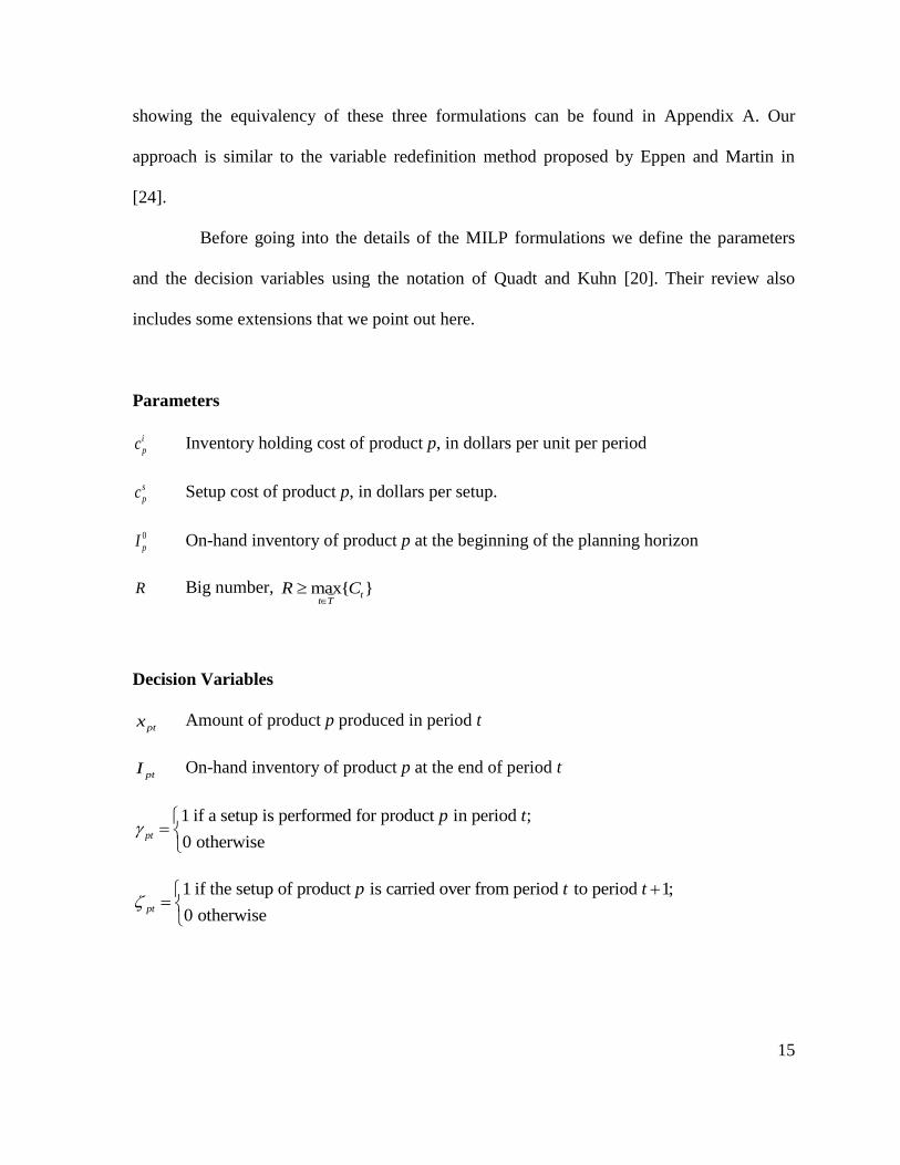
Parameters

i

pc Inventory holding cost of product p, in dollars per unit per period

s

pc Setup cost of product p, in dollars per setup.

0

pI On-hand inventory of product p at the beginning of the planning horizon

R Big number, max{ }tt T

R C

Decision Variables

ptx Amount of product p produced in period t

ptI On-hand inventory of product p at the end of period t

1 if a setup is performed for product in period ;

0 otherwisept

p t

1 if the setup of product is carried over from period to period 1;

0 otherwisept

p t t

16

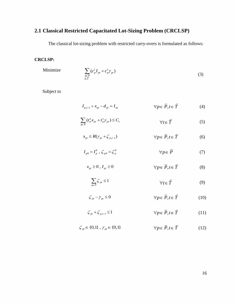
2.1 Classical Restricted Capacitated Lot-Sizing Problem (CRCLSP)

The classical lot-sizing problem with restricted carry-overs is formulated as follows:

CRCLSP:

Minimize ( )i s

p pt p pt

p Pt T

c I c

(3)

Subject to

, 1p t pt pt ptI x d I ,p P t T (4)

( )u s

p pt p pt t

p P

t x t C

t T (5)

, 1( )pt pt p tx R ,p P t T (6)

0 0

0 0 , p p p pI I p P (7)

0 , 0pt ptx I ,p P t T (8)

1pt

p P

t T (9)

0pt pt ,p P t T (10)

, 1 1pt p t ,p P t T (11)

{0,1} , {0,1}pt pt ,p P t T (12)

17

This CRCLSP formulation minimizes the total holding and setup cost. As we

mentioned earlier, we assume that holding cost is not significant in the motivating context

(transactional print shops), and therefore in this case, 0, i

pc p . Constraint (4) is the

inventory balance equation. Constraint (5) limits the sum of total setup time and total

processing time in period t according to capacity available in the corresponding period.

Constraint (6) assures that the machine is either set up or the setup is carried over from the

previous period if there is production of product p in period t. Constraint (7) establishes the

initial inventory and setup state. In our case we assume that the initial inventory is zero since

we consider a make-to-order system. We assume that 0 0,p p meaning that no setup has

been carried over from previous periods to the first period of the problem. In other words, the

machine is not set up for any product at the beginning of the planning horizon. Constraint (9)

ensures that no more than one setup is carried over from one period to the next. Constraint

(10) implies that the machine has to be set up in a period to be able to carry that setup to the

next period. Constraint (11) implies that the setup can be carried over to the next adjacent

period but not further.

2.2 Modified Restricted CLSP (Capacitated Lot-Sizing Problem)

The classical restricted formulation with setup carry-over can be modified so that it

yields improved performance in terms of computation time. This formulation is the extended

version of the formulation proposed by Haase [17]. We extend it by including setup times in

the capacity constraint because, different from his formulation, setups consume capacity in

18

our problem. Although the number of variables remains the same, the average computation

time of this modified formulation is significantly less than that of the classical formulation.

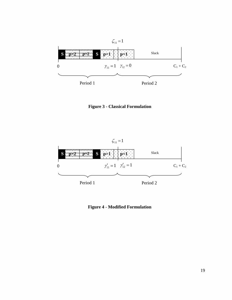
In this formulation we redefine the setup variable pt and change the notation

slightly. We replace the variable pt in the classical formulation with the variable 'pt . While

pt represents the setup state pt represents the production state. In other words, if a product

p is produced in period t then 1pt , else 0pt .

Figure 3 and Figure 4 below show the difference between the two variables pt and

pt . In both situations, a setup for product p=1 is carried over from the first period to the

second. Because the setup is carried over, the variable 12 in the classical formulation is

equal to zero since there is not a set-up for product 1 in period 2. However the variable 12 in

the modified formulation is equal to one since it does not represent the setup state but the

production state of product p.

19

S p=1 S p=2 p=1 p=2

Period 1 Period 2

C1

C1 + C2

0

Slack

11 1 12 1

11 1

Figure 4 - Modified Formulation

S p=1 S p=2 p=1 p=2

Period 1 Period 2

C1

C1 + C2

0

Slack

11 1 12 0

11 1

Figure 3 - Classical Formulation

20

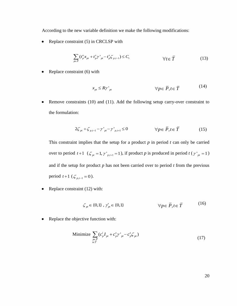
According to the new variable definition we make the following modifications:

Replace constraint (5) in CRCLSP with

, 1( ' )u s s

p pt p pt p p t t

p P

t x t t C

t T (13)

Replace constraint (6) with

'pt ptx R ,p P t T (14)

Remove constraints (10) and (11). Add the following setup carry-over constraint to

the formulation:

, 1 , 12 ' ' 0pt p t pt p t ,p P t T (15)

This constraint implies that the setup for a product p in period t can only be carried

over to period 1t (, 11, ' 1pt p t ), if product p is produced in period t ( ' 1pt )

and if the setup for product p has not been carried over to period t from the previous

period 1t (, 1 0p t ).

Replace constraint (12) with:

{0,1} , {0,1}pt pt ,p P t T

(16)

Replace the objective function with:

Minimize

( ' )i s s

p pt p pt p pt

p Pt T

c I c c

(17)

21

We modify the objective function to take into account the setup cost saving due to

setup carry-over. The complete formulation is as follows:

Modified Restricted CLSP (MRCLSP)

Minimize 1( ' )i s s

p pt p pt p pt

p Pt T

c I c c

(17)

Subject to

, 1p t pt pt ptI x d I ,p P t T (4)

, 1'u s s

p pt p pt p p t t

p P

t x t t C

t T (13)


0 0

0 0 , p p p pI I p P (7)

0 , 0pt ptx I ,p P t T (8)

1pt

p P

t T (9)

, 1 , 12 ' ' 0pt p t pt p t ,p P t T

(15)

' {0,1} , {0,1}pt pt ,p P t T

(16)

22

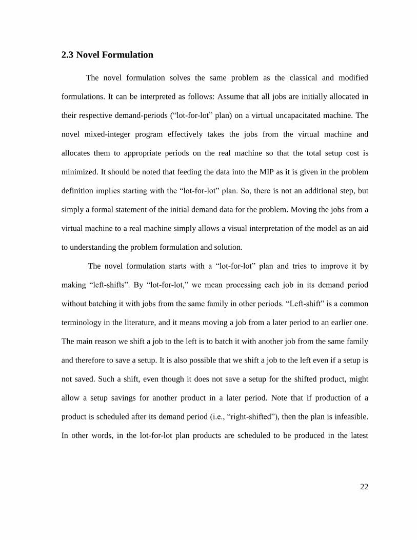
2.3 Novel Formulation

The novel formulation solves the same problem as the classical and modified

formulations. It can be interpreted as follows: Assume that all jobs are initially allocated in

their respective demand-periods (―lot-for-lot‖ plan) on a virtual uncapacitated machine. The

novel mixed-integer program effectively takes the jobs from the virtual machine and

allocates them to appropriate periods on the real machine so that the total setup cost is

minimized. It should be noted that feeding the data into the MIP as it is given in the problem

definition implies starting with the ―lot-for-lot‖ plan. So, there is not an additional step, but

simply a formal statement of the initial demand data for the problem. Moving the jobs from a

virtual machine to a real machine simply allows a visual interpretation of the model as an aid

to understanding the problem formulation and solution.

The novel formulation starts with a ―lot-for-lot‖ plan and tries to improve it by

making ―left-shifts‖. By ―lot-for-lot,‖ we mean processing each job in its demand period

without batching it with jobs from the same family in other periods. ―Left-shift‖ is a common

terminology in the literature, and it means moving a job from a later period to an earlier one.

The main reason we shift a job to the left is to batch it with another job from the same family

and therefore to save a setup. It is also possible that we shift a job to the left even if a setup is

not saved. Such a shift, even though it does not save a setup for the shifted product, might

allow a setup savings for another product in a later period. Note that if production of a

product is scheduled after its demand period (i.e., ―right-shifted‖), then the plan is infeasible.

In other words, in the lot-for-lot plan products are scheduled to be produced in the latest

23

possible period. The lot-for-lot plan might not be feasible due to capacity limitations, but if

there is a feasible plan then the novel formulation makes necessary left-shifts and finds it.

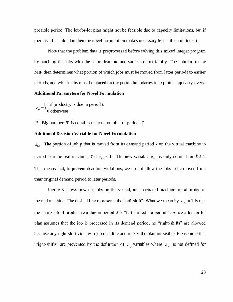
Note that the problem data is preprocessed before solving this mixed integer program

by batching the jobs with the same deadline and same product family. The solution to the

MIP then determines what portion of which jobs must be moved from latter periods to earlier

periods, and which jobs must be placed on the period boundaries to exploit setup carry-overs.

Additional Parameters for Novel Formulation

1 if product is due in period ;

0 otherwisetp

p ty

R : Big number R is equal to the total number of periods T

Additional Decision Variable for Novel Formulation

tkpz : The portion of job p that is moved from its demand period k on the virtual machine to

period t on the real machine, 0 1tkpz . The new variable tkpz is only defined for k t .

That means that, to prevent deadline violations, we do not allow the jobs to be moved from

their original demand period to later periods.

Figure 5 shows how the jobs on the virtual, uncapacitated machine are allocated to

the real machine. The dashed line represents the ―left-shift‖. What we mean by 122 1z is that

the entire job of product two due in period 2 is ―left-shifted‖ to period 1. Since a lot-for-lot

plan assumes that the job is processed in its demand period, no ―right-shifts‖ are allowed

because any right-shift violates a job deadline and makes the plan infeasible. Please note that

―right-shifts‖ are prevented by the definition of tkpz variables where

tkpz is not defined for

24

k t . The other three vertical lines demonstrate that those jobs are not left-shifted and will

be produced in their demand-periods.

Figure 6 – Optimal Solution

Figure 5 – Left-Shift

S

S p=1 S p=2 p=1 p=2

Period 1 Period 2

C1

C1 + C2

0

Slack

S

S p=1 S p=2 S p=1 p=2

Period 1 Period 2

Infinite

capacity

Infinite

capacity

0

Infinite

Slack

Infinite

Slack

111 1z

111 1z

112 1z

111 1z

122 1z

111 1z

221 1z

111 1z

Virtual Machine

Real Machine

Left-Shift

S p=1 S p=2 p=1 p=2

Period 1 Period 2

C1

C1 + C2

0

Slack

Real Machine

25

Figure 6 shows how the plan looks after the job for product 2, due in period 2 is left-

shifted from period 2 to period 1. If the sequence of the jobs in period 1 is changed, the setup

for product 1 in period 1 can be carried over to period 2. In that case the plan looks like

Figure 6. This is optimal because we know that there has to be at least one setup for each

product. Since we have two products to produce, the plan with two setups has to be optimal.

Novel Formulation for CLSP

NMCLSP

Minimize 1( ' )s s

p pt p pt

p Pt T

c c

(18)

Subject to

, 1'u s s

p tkp pk p pt p p t t

p P k T

t z d t t C

t T

(19)

' 'tkp pt

k T

z R

,p P t T (20)

1pt

p P

t T

(21)

, 1 , 12 ' ' 0pt ptp t p t

,p P t T

(22)

tkp kp

t T

z y

,p P k T

(23)

0

0p p p P (24)

26

0 1tkpz , ,p P t T k T (25)

{0,1} , ' {0,1}pt pt

,p P t T (26)

Constraint (19) assures that capacity conditions are met. Constraint (20) forces a

setup for product p in period t if any job is moved into period t of the real machine from the

virtual machine. Constraints (21) and (22) take care of setup carry-overs as described in the

previous section on the modified formulation with setup carry-overs. Constraint (23) ensures

that all the jobs on the virtual machine are moved to the real machine. In other words, this

constraint makes sure that the demand is satisfied. Note that the formulation does not allow

production of more than the total demand because we know that in an optimal solution this is

never the case since we assume a make-to-order environment. Constraint (24) defines the

initial setup state. We assume that 0 0p , meaning that no setup has been carried over to

the first period. Constraint (25) defines the boundaries of variable tkpz . Constraint (26) is the

integrality constraint for the other variables. The objective function of the novel formulation

is the same as the objective function of the modified formulation; both are minimizing the

total setup cost. We do not track inventory levels in this version of the novel formulation.

Hence, there are no inventory variables. In next chapter, we extend the novel formulation so

that it includes inventory holding costs in the objective function and therefore inventory

variables are needed to track the inventory levels.

Our novel formulation can also be interpreted as a fixed charge network flow

formulation of the lot-sizing problem. Figure 7 shows the fixed charge network flow

27

interpretation of our novel formulation for a single product for a three-period problem. Nodes

1, 2 and 3 represent the first three periods of the problem. Arcs (0,t) represent demands due

in period t. They ensure that the problem starts with the lot-for-lot plan. Arcs (t,4) represent

the production in period t and the flow of these arcs are given by the variable ptx . The

variable ptx represents the sum of processing times and the setup times in period t. In a

feasible solution, the capacity constraint requires that ,pt t

p P

x C t

. It can be said that node

4 is the coupling node since different networks of different products are connected to each

other through this node. It should be noted that in this fixed charge network flow diagram we

do not show the variables tkpz where t=k since arcs (0,t) already represent them.

Figure 7 - Fixed Charge Network Flow Interpretation of Novel Formulation

0

1

2

3

4

1px

2px

3px

d1

d2

d3

d2*z12

d3*z23

d3*z13

1

s

pt (Cost: s

pc )

3

s

pt (Cost:s

pc )

(cost: S)

1

s

pt (Cost:-s

pc )

2

s

pt (Cost:-s

pc )

2

s

pt (Cost:s

pc )

28

2.4 Computational Experiments

In this section, first we explain how sample instances are generated for test purposes

and then report the results of these computational experiments, followed by performance

evaluations of the different formulations.

Density and slackness t are two important characteristics of demand structure and

both parameters are defined formally in Section 1.3. Other than these two parameters,

number of periods, number of job families, job-size distribution and setup times are also

significant problem characteristics.

In the first computational experiment, we assume that the processing times of jobs are

uniformly distributed between 100 and 200. In the second experiment, we sample the

processing times from two different uniform distributions to mimic the ―skewed‖

characteristic of the real-world demand. The details of the mixture distribution are explained

in Section 2.4.2. The MIPs have been formulated to allow disparate setup times across jobs.

In our initial tests, however, we have assumed that the setup time for each job is the same.

Based on our experience, this assumption is reasonable in the print-shop environment that

motivated our work. In our experimental design we have four different levels of setup.

Details of the experimental design are shown in Table 1.

29

Table 1 - Sample Problem Characteristics

Parameter Values of Different Levels

T Number of Periods 5

P Number of Job Families 60, 100, 140

Density 0.5, 0.7, 0.9

t Slackness 0, 0.25, 0.5

s

pt Setup time 10, 50, 100, 200

tC Period Length (capacity)

1

u s

p pt p pt

p P

t

t d t y

u

p ptt d Job Size [100,200]U

We have a 3×3×3×4 full factorial design, and we generate 10 instances for each

combination. So, in total, 1080 instances are solved using the three different formulations.

All formulations are generated in Matlab 2010a and CPLEX 12.2 is used as the solver. We

limit the number of active threads in CPLEX to one. Other than that, the CPLEX default

settings are used. All experiments were run on a PC with an Intel Xeon 2.67 GHz CPU and 3

GB RAM.

2.4.1 Experiment with the Uniform Processing Times

In the first experiment processing times are generated using a single uniform

distribution, [100,200]U . After we show how the sample instances are generated we present

the results from three formulations.

30

2.4.1.1 Sample Instance Generation (Uniform Distribution)

Before presenting the algorithm used to generate sample instances, we must define a

new parameter:

[ ]tE

For our experiments, is calculated simply by taking the average of t . In addition, s

pt is

fixed and , s s

pt t p meaning that [ ]s s

pE t t . In other words, setup time is the same for all

products. Also u

p ptt d is uniformly distributed between 100 and 200 implying that

[ ] 150u

p ptE t d . Microsoft Excel 2007 and its standard functions are used to generate sample

problems.

The following procedure is used to generate sample problems for given values of and :

STEP 1: Generate a T × P matrix with random numbers [0,1]U in each cell.

STEP 2: If the random number in a cell is greater than , then set the cell value

equal to 0, otherwise generate a processing time u

pt from [100,200]U .

STEP 3: Set [ ] [ ]

, 1

u s

p pt p

t

P E t d E tC t

.

Table 2 and Table 3 present descriptive statistics of the slackness and density values

of the generated instances.

31

Table 2 - Test Bed Statistics (Slackness)

0 0.25 0.5

P Min Max Mean Min Max Mean Min Max Mean

60 -0.06 0.15 0.03 0.14 0.37 0.25 0.44 0.58 0.50

100 -0.04 0.12 0.02 0.19 0.34 0.25 0.42 0.55 0.50

140 -0.03 0.09 0.02 0.20 0.31 0.25 0.45 0.55 0.50

Table 3 - Test Bed Statistics (Density)

0.5 0.7 0.9

P Min Max Mean Min Max Mean Min Max Mean

60 0.41 0.57 0.49 0.63 0.75 0.69 0.84 0.94 0.90

100 0.44 0.58 0.49 0.62 0.74 0.70 0.82 0.93 0.89

140 0.45 0.55 0.50 0.65 0.74 0.70 0.86 0.93 0.90

2.4.1.2 Experimental Results

We have two measures of solution performance: computation time and the percentage

gap between the upper and lower bounds of the branch & bound tree. We report the default

gap value returned by the CPLEX engine. The gap is defined as follows:

100%.UB LB

UB

z z

z

The term UBz defines the objective value of the current best integer solution (incumbent

solution) while *

LBz represents the objective value of the LP relaxation optimal solution

obtained for the current best node in the branch and bound tree.

32

We stop the solution engine after 1200 seconds and return the best solution found up

to that point. We assume that in most real production environments, where production plans

are regenerated frequently (e.g., every day or every shift), a computation time greater than

1200 seconds is not very practical. The other reason is the limited memory of personal

computers. As expected, as the maximum computation time goes up, the more likely it is that

the solution procedure will abort due to insufficient memory.

Table 4 shows the means, medians and standard errors of computation times (i.e., the

standard deviation of the mean computation time, given by the sample standard deviation

divided by the square root of the number of observations) for different formulations and

different numbers of products. Please note that for each product level we solve 360 instances

with a planning horizon of 5 periods. Clearly, the classic formulation performs worst among

these three formulations.

Table 4 - Computation Time Summary, Single Machine, Uniform Processing Times

Time (s)

Classic Formulation Modified Formulation Novel Formulation

P Mean Std. Error Median Mean Std. Error Median Mean Std. Error Median

60 289 26 5 128 18 2 30 9 1

100 492 30 50 288 25 10 79 13 5

140 595 30 354 472 29 38 165 19 13

33

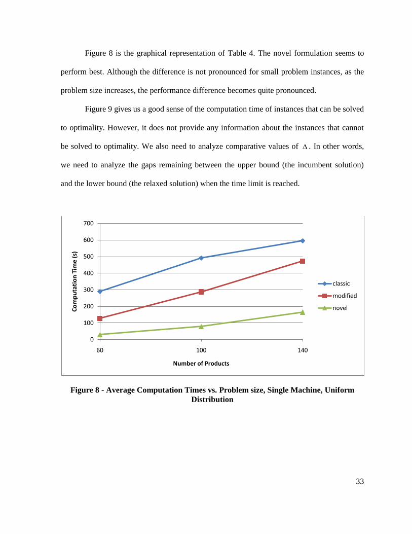
Figure 8 is the graphical representation of Table 4. The novel formulation seems to

perform best. Although the difference is not pronounced for small problem instances, as the

problem size increases, the performance difference becomes quite pronounced.

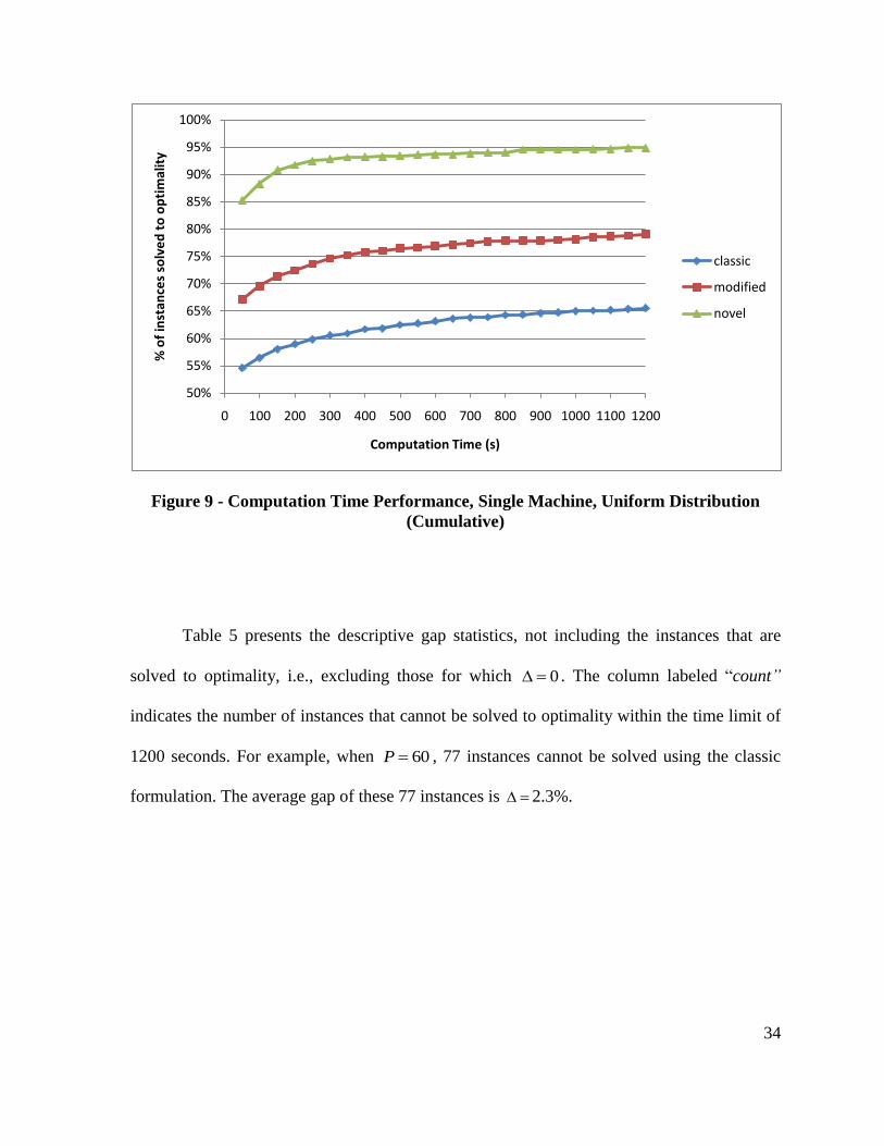
Figure 9 gives us a good sense of the computation time of instances that can be solved

to optimality. However, it does not provide any information about the instances that cannot

be solved to optimality. We also need to analyze comparative values of . In other words,

we need to analyze the gaps remaining between the upper bound (the incumbent solution)

and the lower bound (the relaxed solution) when the time limit is reached.

Figure 8 - Average Computation Times vs. Problem size, Single Machine, Uniform

Distribution

0

100

200

300

400

500

600

700

60 100 140

Co

mp

uta

tio

n T

ime

(s)

Number of Products

classic

modified

novel

34


(Cumulative)

Table 5 presents the descriptive gap statistics, not including the instances that are

solved to optimality, i.e., excluding those for which 0 . The column labeled ―count”

indicates the number of instances that cannot be solved to optimality within the time limit of

1200 seconds. For example, when 60P , 77 instances cannot be solved using the classic

formulation. The average gap of these 77 instances is 2.3%.

50%

55%

60%

65%

70%

75%

80%

85%

90%

95%

100%

0 100 200 300 400 500 600 700 800 900 1000 1100 1200

% o

f in

stan

ces

solv

ed

to

op

tim

alit

y

Computation Time (s)

classic

modified

novel

35

Table 5 - Gap Summary, Single Machine, Uniform Processing Times

(Gap)


P Count Mean Std. Error Max Count Mean Std. Error Max Count Mean Std. Error Max

60 77 2.3% 0.16% 5.6% 29 1.4% 0.14% 4.3% 7 0.9% 0.08% 1.1%

100 128 1.4% 0.10% 5.6% 69 0.8% 0.04% 1.8% 15 0.5% 0.04% 0.8%

140 165 1.1% 0.07% 5.4% 125 0.7% 0.03% 2.7% 33 0.4% 0.04% 1.2%

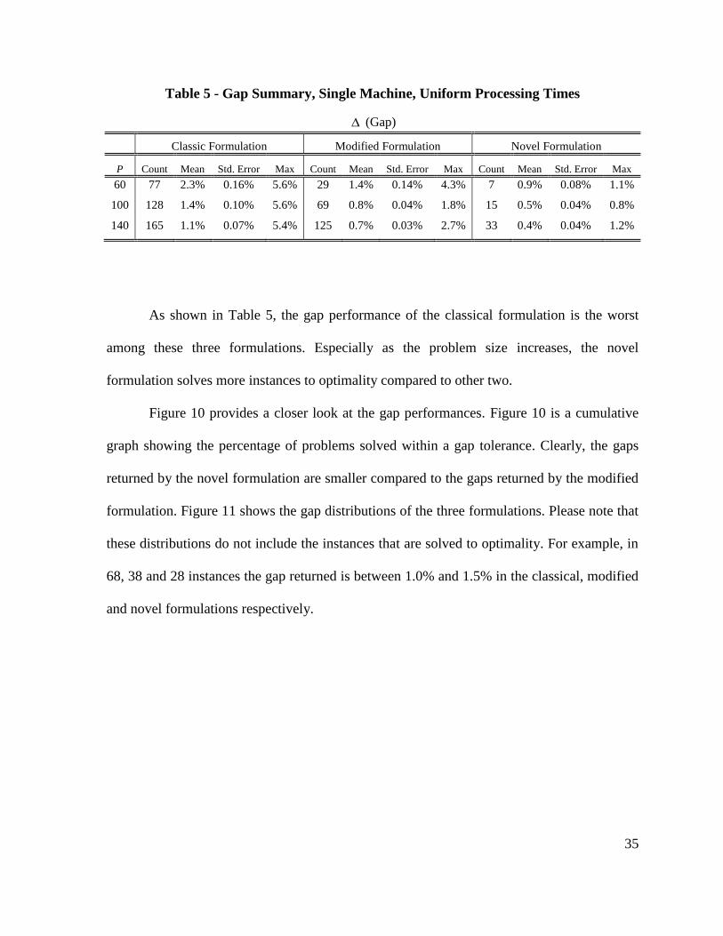
As shown in Table 5, the gap performance of the classical formulation is the worst

among these three formulations. Especially as the problem size increases, the novel

formulation solves more instances to optimality compared to other two.

Figure 10 provides a closer look at the gap performances. Figure 10 is a cumulative

graph showing the percentage of problems solved within a gap tolerance. Clearly, the gaps

returned by the novel formulation are smaller compared to the gaps returned by the modified

formulation. Figure 11 shows the gap distributions of the three formulations. Please note that

these distributions do not include the instances that are solved to optimality. For example, in

68, 38 and 28 instances the gap returned is between 1.0% and 1.5% in the classical, modified

and novel formulations respectively.

36

Figure 10 - Gap Performance, Single Machine, Uniform Distribution (Cumulative)

Figure 11 - Gap Distribution, Single Machine, Uniform Processing Times

65%

70%

75%

80%

85%

90%

95%

100%

0.0% 0.5% 1.0% 1.5% 2.0% 2.5% 3.0% 3.5% 4.0% 4.5% 5.0%

% o

f in

stan

ces

solv

ed

Δ (Gap)

classic

modified

novel

0

20

40

60

80

100

120

140

Nu

mb

er

of

Inst

ance

s

∆ (Gap)

classic

modified

novel

37

Both figures confirm the conclusion that the classic formulation performs the worst

and the novel formulation performs the best among these three formulations. The

performance of the modified formulation and the novel formulation does not differ by much

when the total number of products is low. However, as the total number of products increases

the novel formulation starts to outperform the modified formulation.

2.4.2 Experiment with the Mixed Processing Times

In the previous experiment, we generated all processing times from a single,

relatively tight uniform distribution. Because of the “knapsack characteristics” of the

problem, that kind of test bed is challenging and academically interesting. However, in real-

life there are different customer types and related order sizes (small vs. large). We know that

the 80-20 rule applies in many situations in practice, and indeed, data from our motivating

problem indicates that approximately 15% of the orders are much larger than the remaining

orders. To test the effect of this demand structure, in this experiment we generate the

processing times from a mixture of distributions. The job-size index is defined as follows:

1 if the job is small

2 if the job is big

,

u

p ptt d represents the processing type of a job. We sample the ―small jobs‖,

,1

u

p ptt d , from

[100,200]U and we arbitrarily define the distribution for the ―big jobs‖ , ,2

u

p ptt d , to be

[1000,1200]U since specific data from the motivating example is difficult to obtain, based on

the multi-stage nature of the process in the motivating environment.

38

2.4.2.1 Sample Instance Generation (Mixture Distribution)

We define a new parameter ( 0 1 ) representing the percentage of products

with high demand. In this experiment 0.15 , meaning that only 15% of the products are

in the high demand category.

The following algorithm is used to generate problem instances:

STEP 1: Generate a T by P matrix with random numbers [0,1]U in each cell.

STEP 2: If the random number in a cell is greater than , then set the cell value

equal to 0 and go to step 3, otherwise generate a random number from [0,1]U . If

is greater than , then 1 , and generate the processing time from [100,200]U ;

else, 2 generate the processing time from [1000,1200]U .

STEP 3: ,1 ,2(1 ) [ ] [ ] [ ]

, 1

u u s

p pt p pt p

t

P E t d E t d E tC t

For our experiments, s

pt is fixed and , s s

pt t p meaning that [ ]s s

pE t t . Also ,1

u

p ptt d

is uniformly distributed between 100 and 200 implying that ,1[ ] 150u

p ptE t d . Similarly,

,2

u

p ptt d is uniformly distributed between 1000 and 1200 meaning that ,2[ ] 1100u

p ptE t d . Since

we set 0.15 in our experiment, ,1 ,2(1 ) [ ] [ ] 292.5u u

p pt p ptE t d E t d . Microsoft Excel

2007 and its standard functions are used to generate sample problems. Microsoft Excel 2007

and its standard functions are used to generate sample problems.

39

2.4.2.2 Experimental Results

We have exactly the same experimental design as the previous experiment except the

processing times. Although only 15% of the products have high demand, it turns out that the

problem gets significantly easier. Table 6 summarizes the mean and median computation

times and the standard errors for different problem sizes. All formulations perform better

with this demand structure compared to the previous experiment where a single uniform

distribution was used. The mean computation times of the classic formulation are

approximately the half of those from the previous experiment, while the mean computation

times of the modified and the novel formulation are approximately one fifth of those from the

previous experiment. That means all formulations perform better but the extent of

improvement is much greater for the modified and novel formulations.

Table 6 - Computation Time Summary, Single Machine, Mixed Processing Times

Time (s)



60 136 19 2 26 8 1 6 3 1

100 241 25 4 51 12 3 9 4 1

140 305 26 9 129 18 5 32 8 2

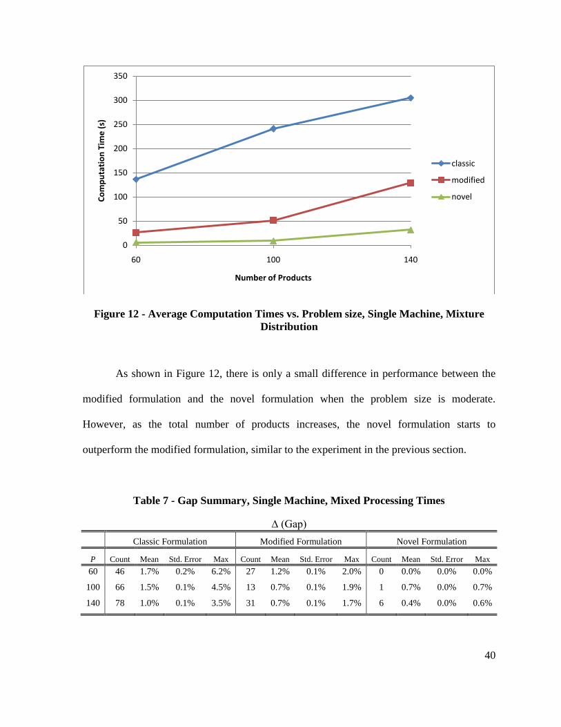
40

Figure 12 - Average Computation Times vs. Problem size, Single Machine, Mixture

Distribution

As shown in Figure 12, there is only a small difference in performance between the

modified formulation and the novel formulation when the problem size is moderate.

However, as the total number of products increases, the novel formulation starts to

outperform the modified formulation, similar to the experiment in the previous section.

Table 7 - Gap Summary, Single Machine, Mixed Processing Times

∆ (Gap)



60 46 1.7% 0.2% 6.2% 27 1.2% 0.1% 2.0% 0 0.0% 0.0% 0.0%

100 66 1.5% 0.1% 4.5% 13 0.7% 0.1% 1.9% 1 0.7% 0.0% 0.7%

140 78 1.0% 0.1% 3.5% 31 0.7% 0.1% 1.7% 6 0.4% 0.0% 0.6%

0

50

100

150

200

250

300

350

60 100 140

Co

mp

uta

tio

n T

ime

(s)

Number of Products

classic

modified

novel

41

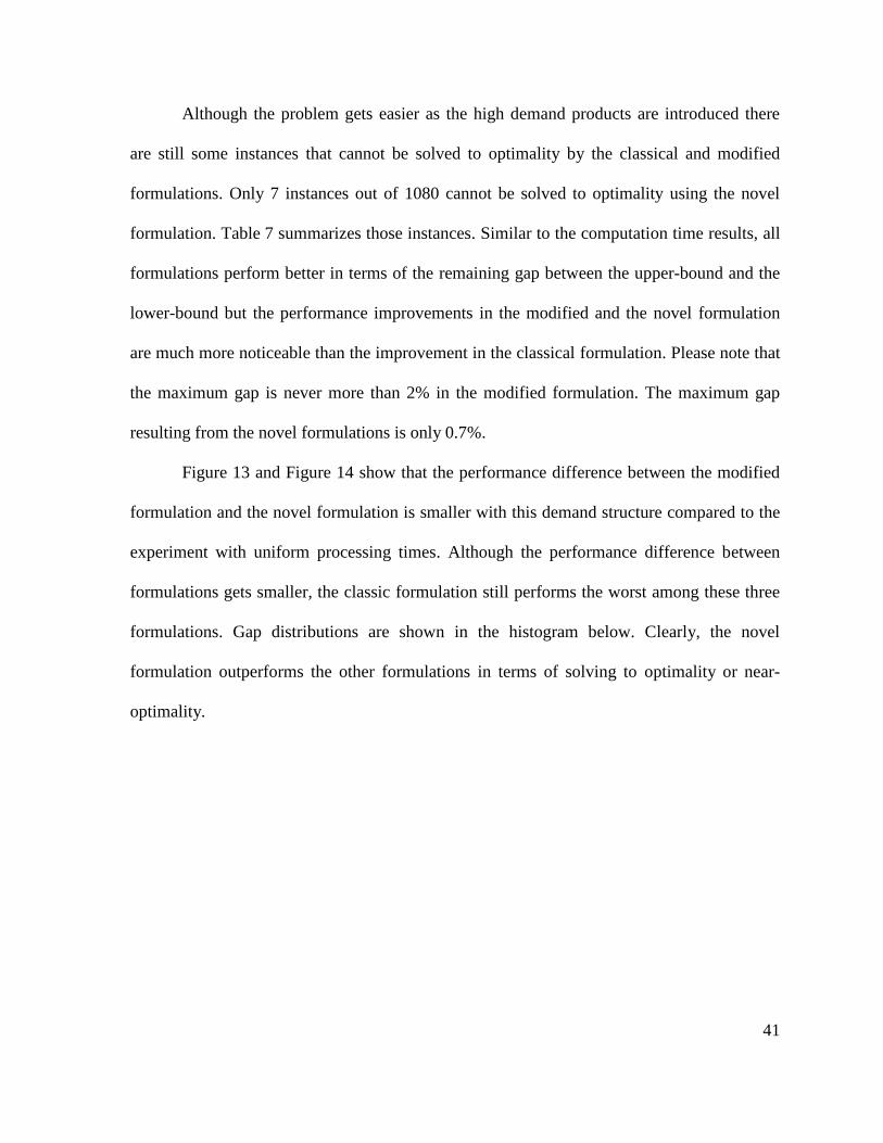
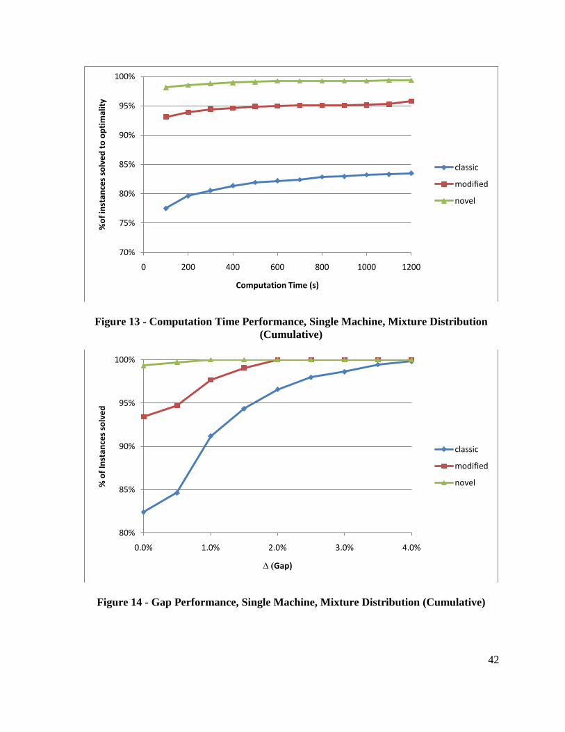
Although the problem gets easier as the high demand products are introduced there

are still some instances that cannot be solved to optimality by the classical and modified

formulations. Only 7 instances out of 1080 cannot be solved to optimality using the novel

formulation. Table 7 summarizes those instances. Similar to the computation time results, all

formulations perform better in terms of the remaining gap between the upper-bound and the

lower-bound but the performance improvements in the modified and the novel formulation

are much more noticeable than the improvement in the classical formulation. Please note that

the maximum gap is never more than 2% in the modified formulation. The maximum gap

resulting from the novel formulations is only 0.7%.

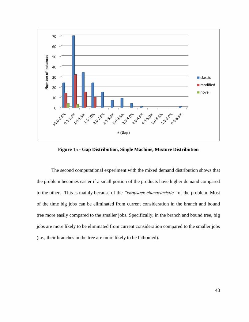
Figure 13 and Figure 14 show that the performance difference between the modified

formulation and the novel formulation is smaller with this demand structure compared to the

experiment with uniform processing times. Although the performance difference between

formulations gets smaller, the classic formulation still performs the worst among these three

formulations. Gap distributions are shown in the histogram below. Clearly, the novel

formulation outperforms the other formulations in terms of solving to optimality or near-

optimality.

42

Figure 13 - Computation Time Performance, Single Machine, Mixture Distribution

(Cumulative)

Figure 14 - Gap Performance, Single Machine, Mixture Distribution (Cumulative)

70%

75%

80%

85%

90%

95%

100%

0 200 400 600 800 1000 1200

%o

f in

stan

ces

solv

ed

to

op

tim

alit

y


classic

modified

novel

80%

85%

90%

95%

100%

0.0% 1.0% 2.0% 3.0% 4.0%

% o

f In

stan

ces

solv

ed

∆ (Gap)

classic

modified

novel

43

Figure 15 - Gap Distribution, Single Machine, Mixture Distribution

The second computational experiment with the mixed demand distribution shows that

the problem becomes easier if a small portion of the products have higher demand compared

to the others. This is mainly because of the “knapsack characteristic” of the problem. Most

of the time big jobs can be eliminated from current consideration in the branch and bound

tree more easily compared to the smaller jobs. Specifically, in the branch and bound tree, big

jobs are more likely to be eliminated from current consideration compared to the smaller jobs

(i.e., their branches in the tree are more likely to be fathomed).

0

10

20

30

40

50

60

70

Nu

mb

er

of

Inst

ance

s

∆ (Gap)

classic

modified

novel

44

2.5 Comparison of the Formulations

In this section, we address the question of why there is a performance difference

between three formulations. We first compare the classical formulation with the modified

formulation and then the modified formulation with the novel formulation.

2.5.1 Classical Formulation vs. Modified Formulation

The main difference between the classical formulation and the modified formulation

is the setup variable pt and the production variable 'pt . In the classical formulation, the

variable pt indicates whether the machine is set up for product p in period t or not.

However, the variable 'pt in the modified formulation only indicates whether product p is

produced in period t or not. Figure 3 and Figure 4 in Section 2.2 show this fundamental

difference visually.

Mathematically, the relationship between these two variables can be represented as

follows: , 1'pt pt p t . Using this variable redefinition, the classical formulation can be

converted to the modified formulation. See Appendix A for further details. It turns out that

this simple variable redefinition simplifies the branch and bound tree significantly.

Let’s assume that we have a single product and we are at some point in the branch

and bound tree. Since we have only one product we can drop the product index p for

convenience. We will branch on t , 1t , t and 1t (or 't , 1't , t and 1t ). Figure 16

and Figure 17 show the portion of the branch and bound tree relevant to period t for the

classical formulation and the modified formulation, respectively. The diamond shaped boxes,

45

labeled ―Inf”, represent the infeasible solutions. Note that this portion of the branch and

bound tree for the classical formulation has 26 nodes in total, while the portion of the tree for

the modified formulation has 24 nodes in total. If we look at the trees carefully, we see that

they are the same except where 1t , 1 0t and 1t . This part of the tree is pruned by

infeasibility in the modified formulation because constraint (15) is violated when ' 1t ,

1' 0t and 1t . More clearly, if we substitute the values of the variables into the

constraint , 1 , 12 ' ' 0pt p t pt p t we get

, 11 0p t , which is always false.

Compared to the classical formulation, the branch and bound tree of the modified

formulation is more compact. The difference might seem small, but this small reduction in

the number of nodes in the branch and bound tree for any given value of p and t has dramatic

effects as the problem size increases (i.e., as T increases, and particularly as P increases). As

we see in the computational experiments, this has a dramatic impact on the computational

performance. In short, it can be said that in the modified formulation a branch in each p-t

region of the tree is pruned by the formulation. Therefore, the branch and bound tree for the

modified formulation has fewer nodes than the branch and bound tree of the classical

formulation.

46

Figure 16 - Branch & Bound Tree of the Classical Formulation

Figure 17 - Branch & Bound Tree of the Modified Formulation

γt=0

γt+1=0

ζt=0

ζt+1=0 inf

inf

γt+1=1

ζt=0

ζt+1=0 ζt+1=1

inf

γt=1

γt+1=0

ζt=0

ζt+1=0 inf

ζt=1

ζt+1=0 inf

γt+1=1

ζt=0

ζt+1=0 ζt+1=1

ζt=1

ζt+1=0 inf

γ't=0

γ't+1=0

ζt=0

ζt+1=0 inf

inf

γ't+1=1

ζt=0

ζt+1=0 ζt+1=1

inf

γ't=1

γ't+1=0

ζt=0

ζt+1=0 inf

inf

γ't+1=1

ζt=0

ζt+1=0 ζt+1=1

ζt=1

ζt+1=0 inf

Pruned in the Modified

Formulation

47

2.5.2 Modified Formulation vs. Novel Formulation

The computational experiments show that if an instance cannot be solved to

optimality, the gap remaining between the upper bound and the lower bound is usually

smaller in the novel formulation compared to the modified formulation. Since the integer

variables are the same in both formulations the branch and bound trees are also the same.

Although the two mixed integer formulations are equivalent to each other, their LP

relaxations are not, as we show below.

Similar to the conversion between the classical formulation and the modified

formulation, we can convert the modified formulation to the novel formulation with the

following variable redefinition:

.tp tkp pk

k T

x z d

All constraints in the modified formulation, other than the one containing the big

number R , can be converted directly to the corresponding constraint in the novel formulation

using the variable redefinition above. That means all constraints in the modified formulation

except constraint (14) are equivalent to the corresponding constraints in the novel

formulation in terms of the LP relaxation. For further details see Appendix A.

To understand the performance difference between the novel formulation and the

modified formulation we need to understand the difference between these two constraints:


' 'tkp pt

k T

z R

,p P t T (20)

48

Constraint (14) appears in the modified formulation and constraint (20) is the corresponding

constraint in the novel formulation. It should be noted that R is equal to the maximum period

capacity in the planning horizon and R is equal to the total number of periods.

In the LP relaxation the integrality constraints are relaxed, so the 'pt variables can

assume fractional values. The closer those fractional values are to unity, the tighter the lower

bounds provided by the LP relaxation.

If we sum the 'pt variables over t, constraint (14) can be written as follows:

.'pt

t Tpt

t T

x

R

(27)

Similarly constraint (20) can be written as follows:

1

T T

tkp

t k tpt

t T

z

R

.

(28)

Because the objective is to minimize total cost, the 'pt variables will assume the

minimum values possible and their lower-bounds are determined by the expressions above.

To see those lower-bounds clearly let’s compare the left-hand side terms of (27) and (28).

We know that in the optimal solution

pt

t T

x

will be no more than the total demand of

product p across all periods. We also know that if pt

t T

x

is less than the total demand then

49

the solution is infeasible, so pt

t T

x

must be equal to the total demand. Since R is equal to the

maximum period capacity (27) can be written as:

maxpt

t Ttt T

total demand for product p

C

(29)

If we assume that processing times of all jobs are sampled from the same distribution,

then expected total demand for a single product p can be written as follows in terms of the

problem parameters:

(1 ) maxTotal demand of a single product

tt T

T C

P

(30)

Substituting (30) into (29) yields:

(1 )pt

t T

T

P

(31)

Finally we sum the expression above over the product families:

(1 ) pt

p P t T

T

(32)

50

It should be noted that the left-hand side of (32) is an expected value and the purpose of (32)

is only to show the relation between problem parameters and the quality of the lower-bound

generated by the LP relaxation.

Similarly (28) can be written as follows:

total number of jobs of product

total number of periodspt

t T

p

(33)

Again, we sum the expression above over p:

total number of jobs

total number of periodspt

p P t T

(34)

Note that the left-hand side of (34) is proportional to the density . While the lower-bound

of the modified formulation is dependent on the length of the planning horizon and the

slackness, the lower bound for the novel formulation is dependent on the density of the

problem.

2.6 Conclusions

In this chapter, we presented three different mixed integer formulations to solve

capacitated lot-sizing problems with setup times and setup carry-overs. As an alternative to

the classical and modified formulations found in the literature we suggest a novel

51

formulation. Table 8 presents the number of integer and continuous variables for each three

formulations.

Table 8 - Number of Variables (No holding cost)

Formulation Number of

Integer Variables

Number of

Continuous Variables

Classical ( 1)TP T P 2TP

Modified ( 1)TP T P 2TP

Novel ( 1)TP T P ( 1)

2

PT T

Extensive computational experiments showed that our novel formulation consistently

outperforms the classical and modified formulations. Experiments also demonstrated that the

modified formulation is superior to the classical formulation. The performance difference

between the classical formulation and modified formulation stems from the fact that the

branch and bound tree of the modified formulation is more compact compared to the branch

and bound tree of the classical formulation. To the best of our knowledge the difference

between these two formulations has not been analyzed previously in the literature.

We know that the branch and bound trees of the modified formulation and our novel

formulation are equivalent because their integer variables are the same. By comparing the

expressions (32) and (34), it can be easily concluded that in most instances the lower-bound

52

provided by the LP-relaxation of our novel formulation is tighter compared to the modified

formulation. The lower-bound characteristics of the formulations have the following

implications.

- Our experiments show that, keeping all else the same, as slackness increases the

computation time and resulting solution gap both increase for the modified

formulation as compared to the novel formulation. (See Appendix C.)

- By comparing the expressions (32) and (34) the following conclusion can be made

regarding the effect of a shorter planning horizon: Keeping everything else the same,

theoretically, there will be a greater decrease in computation time and solution gap

driven by the length of the planning horizon for the novel formulation compared to

the modified formulation.


regarding the effect of a lower density: Keeping everything else the same,


driven by the lower density for the modified formulation compared to the novel

formulation.

It should be also noted that, for problem instances with planning horizons of 3T

periods, the novel formulation has more continuous variables compared to the other

formulations. Interestingly, however, our results show that the greater number of continuous

variables appears not to be as much of a factor in the computational performance of the

formulation as the quality of lower bound that results from this formulation.

53

CHAPTER 3

3 SINGLE-MACHINE FORMULATIONS

WITH HOLDING COST

In Chapter 2, we propose a novel formulation to solve capacitated lot-sizing problems

with setup carry-overs and show that this novel formulation outperforms the existing

formulations in the literature. However, we did not take inventory holding costs into

consideration due to the nature of the motivating case (i.e. transactional print-shops).

In this section, we generalize the novel formulation to include inventory holding

costs. After extending the formulation, we compare it to formulations in the literature like we

did in Chapter 2. Our results suggest that the generalized version of the novel formulation

outperforms the existing formulations in the literature.

54

3.1 Extending the Novel Formulation

We introduce the following variables and parameters to address the inventory holding

cost. These are the same variables and parameters that we use in the classical and modified

formulations.

ptI : On-hand inventory of product p at the end of period t

0

pI : On-hand inventory of product p at the beginning of the planning horizon

i

pc : Inventory holding cost of product p

As the first step, the objective function (18) is replaced by the new objective function:

Minimize 1( ' )i s s

p pt p pt p pt

p Pt T

c I c c

(35)

After adding i

p ptc I term to the objective function, we add the following constraint to

the novel formulation:

, 1p t tkp pk pt pt

k T

I z d d I

,p P t T (36)

0

0 p pI I

p P (37)

0ptI

,p P t T (38)

55

Constraint (36) is the inventory balance equation and its interpretation is the same as

the inventory balance equations in the other formulations. Constraint (37) sets the initial

inventory level and constraint (38) ensures that the inventory level for a given product and

period is never negative.

3.2 Computational Experiment Results

We conduct computational experiments to compare our novel formulation against the

classical formulation and the modified formulation. We use the test bed used by Trigeiro et

al. [11]. Note that we do not ignore holding costs anymore. In other words, the novel

formulation is now generalized by including inventory variables and holding cost

coefficients. In addition to that, the setup times and setup costs for different products may be

different.

In this test bed there are 751 instances in total, ranging from 4 products to 30 products

and from 15 periods to 30 periods. Compared to the instances that we solve in Section 2.4.1

and in Section 2.4.2, these instances have relatively longer planning horizons and relatively

fewer product families. The slackness values of the instances range from -0.29 to 0.32 with a

mean of 0.06. The density values of the instances range from 0.68 to 1.0 with a mean of 0.9.

We use the same settings, computers and software as we reported in Section 2.4.

Maximum computation time is again limited to 1200 seconds. After reaching the

computation time limit or after running out of memory, the best solution found up to that

point (upper-bound and lower-bound) is returned. Table 9 summarizes the computation time

performance of three different formulations. The average computation times of the modified

56

and novel formulations are clearly lower than the average computation time of the classical

formulation. The median computation time of the novel formulation is the best among these

three formulations.

Table 9 - Computation Time Summary, Single Machine, Trigeiro Test bed

Time (s)


Mean 775.1 599.7 597.9

Std. Error 20.3 21.2 21.2

Median 1200.0 406.4 339.1

Figure 18 - Computation Time Performance, Single Machine, Trigeiro Test Bed

(Cumulative)

20%

25%

30%

35%

40%

45%

50%

55%

60%

0 100 200 300 400 500 600 700 800 900 1000 1100 1200

% o

f in

stan

ces

solv

ed

to

op

tim

alit

y


classic

modified

novel

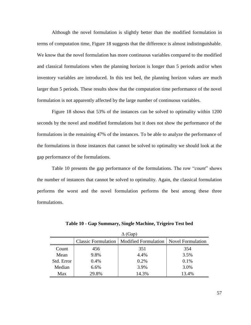
57

Although the novel formulation is slightly better than the modified formulation in

terms of computation time, Figure 18 suggests that the difference is almost indistinguishable.

We know that the novel formulation has more continuous variables compared to the modified

and classical formulations when the planning horizon is longer than 5 periods and/or when

inventory variables are introduced. In this test bed, the planning horizon values are much

larger than 5 periods. These results show that the computation time performance of the novel

formulation is not apparently affected by the large number of continuous variables.

Figure 18 shows that 53% of the instances can be solved to optimality within 1200

seconds by the novel and modified formulations but it does not show the performance of the

formulations in the remaining 47% of the instances. To be able to analyze the performance of

the formulations in those instances that cannot be solved to optimality we should look at the

gap performance of the formulations.

Table 10 presents the gap performance of the formulations. The row ―count‖ shows

the number of instances that cannot be solved to optimality. Again, the classical formulation

performs the worst and the novel formulation performs the best among these three

formulations.

Table 10 - Gap Summary, Single Machine, Trigeiro Test bed

∆ (Gap)


Count 456 351 354

Mean 9.8% 4.4% 3.5%

Std. Error 0.4% 0.2% 0.1%

Median 6.6% 3.9% 3.0%

Max 29.8% 14.3% 13.4%

58

Figure 19 - Gap Performance, Single Machine, Trigeiro Test Bed (Cumulative)

Figure 19 presents the gap performance. This is a cumulative graph showing the

percentage of instances solved within a certain gap tolerance. For example, 67%, 84% and

91% of the 751 instances can be solved within a 5% gap level using the classical, modified

and novel formulations, respectively. Figure 19 also confirms that the novel formulation has

the best gap performance compared to the other two formulations.

40%

50%

60%

70%

80%

90%

100%

0.0% 2.5% 5.0% 7.5% 10.0% 12.5% 15.0% 17.5% 20.0% 22.5% 25.0%

% o

f in

stan

ces

solv

ed

∆ (Gap)

classic

modified

novel

59

Figure 20 - Gap Distribution, Single Machine, Trigeiro Test Bed

By analyzing Figure 20 it can be easily concluded that the gap distribution of the

novel formulation is much better than the other two formulations. After solving all 751

instances using three different formulations we see that the novel formulation performs the

best, although it has more continuous variables. As we show in Section 2.5.2, the main

reason for that is the higher quality of the lower-bounds provided by the LP relaxation of the

novel formulation.

0

20

40

60

80

100

120

140

Nu

mb

er

of

Inst

ance

s

∆ (Gap)

classic

modified

novel

60

3.3 Conclusions

In this chapter we extended our novel formulation by including holding cost. We used

the test bed used by Trigeiro et al. [11] to evaluate the performance of our novel formulation.

Table 11 shows the number of integer and continuous variables for the formulations. Note

that we introduced new inventory variables to the novel formulation and the number of

variables stayed the same for the classical and modified formulations.

Table 11 - Number of Variables (with holding cost)

Formulation Number of

Integer Variables

Number of

Continuous Variables

Classical ( 1)TP T P 2TP

Modified ( 1)TP T P 2TP

Novel

( 1)TP T P

11

2

TTP

Although the number of continuous variables of the novel formulation is greater than

the number of continuous variables of the classical and modified formulations, the

performance of the novel formulation is still better in terms of the percentage gap. The

average computation time values of the novel and modified formulations are much smaller

than the classical formulation. These results are consistent with our conclusions from the

61

previous chapter. The novel formulation performs the best and the classical formulation the

worst among the three formulations we presented.

62

CHAPTER 4

4 PARALLEL-MACHINE FORMULATIONS

The formulations in previous chapters are developed to solve single-machine

problems. In this chapter we extend those formulations so that they can also address parallel-

machine problems. In these formulations, we assume that jobs can be processed on any of

2m machines, all of which process equivalent jobs at the same rate. A job can be allocated

to any of these parallel machines. The machines can be either identical or non-identical in

terms of their capacities. It should be noted that the problem we are solving is still a single-

level problem, meaning that there is only a single operation required to produce the final

product.

In the next three sections we present the extended formulations. All of the extensions

are straightforward. We introduce a new index representing the ―machine-dimension‖. After

developing the formulations, we summarize the results of different computational

63

experiments. These results are consistent with the single-machine experiments. It is clear that

the novel formulation performs the best and the classical formulation the worst among the

three formulations. Although our results appear to indicate that all three formulations

perform poorly in the parallel machine experiments, the integer solutions they provide are

actually good solutions, when compared to a better bound. In Section 4.5, we develop an

improved lower bound and show that the incumbent solutions reported by CPLEX, using all

three formulations, are actually high-quality solutions. In other words, we demonstrate that

what causes the large gaps is the lower bound used by CPLEX.

Because the number of integer variables is large in the parallel-machine problems, we

frequently face memory related issues in attempting to solve the problems. In addition, the

computation times are much higher than for the single-machine problems. In most real-world

situations, however, what really matters is the quality of the best upper-bound attainable

within a reasonable amount of computational time. In other words, proving optimality is not

a major concern for most practitioners, as long as a demonstrably good solution can be

generated with a small or moderate amount of computational effort. To address these

concerns we develop a mathematical programming-based heuristic in Section 4.6. The

purpose of this heuristic is to get high quality upper-bounds in a limited time. Our

experiments suggest that the heuristic performs very well, meaning that it provides high

quality solutions, very quickly compared to the pure MIP approaches.

64

4.1 Classical Restricted Capacitated Lot-Sizing Problem with Parallel

Machines

We start with the classical restricted CLSP, as we did in Chapter 2. Different than the

single machine case, however, we also need to determine on which machine the product is

going to be produced. To be able to extend the formulation to include that decision, we need

to define a new index. Specifically,

m machine index

M total number of machines

In addition to the indices p and t, the decision variables ptx ,

pt and pt must also

include the index m in the parallel-machine formulation. The inventory variables ptI do not

have to be extended by dimension m, because there is no need to track inventories separately

by machine. The parallel-machine extension of the classical restricted CLSP formulation

with restricted carry-overs is as follows:

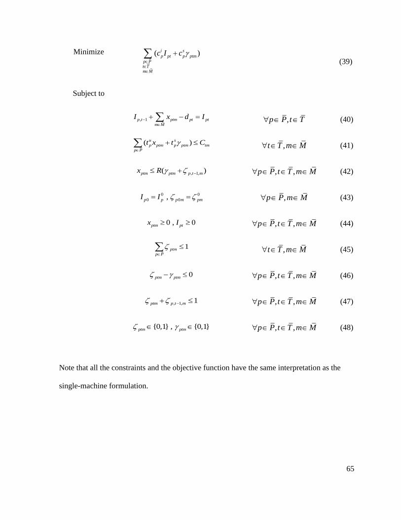
65

Minimize ( )i s

p pt p ptm

p Pt Tm M

c I c

(39)

Subject to

, 1p t ptm pt pt

m M

I x d I

,p P t T (40)

( )u s

p ptm p ptm tm

p P

t x t C

,t T m M (41)

, 1,( )ptm ptm p t mx R , ,p P t T m M (42)

0 0

0 0 , p p p m pmI I ,p P m M (43)

0 , 0ptm ptx I , ,p P t T m M (44)

1ptm

p P

,t T m M (45)

0ptm ptm , ,p P t T m M (46)

, 1, 1ptm p t m , ,p P t T m M (47)

{0,1} , {0,1}ptm ptm , ,p P t T m M (48)

Note that all the constraints and the objective function have the same interpretation as the

single-machine formulation.

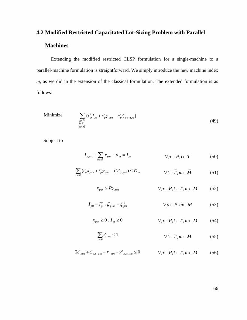
66

4.2 Modified Restricted Capacitated Lot-Sizing Problem with Parallel

Machines

Extending the modified restricted CLSP formulation for a single-machine to a

parallel-machine formulation is straightforward. We simply introduce the new machine index

m, as we did in the extension of the classical formulation. The extended formulation is as

follows:

Minimize , 1,( )i s s

p pt p ptm p p t m

p Pt Tm M

c I c c

(49)

Subject to

, 1p t ptm pt pt

m M

I x d I

,p P t T (50)

, 1( )u s s

p ptm p ptm p p t tm

p P

t x t t C

,t T m M (51)

ptm ptmx R , ,p P t T m M (52)

0 0

0 0 , p p p m pmI I ,p P m M (53)

0 , 0ptm ptx I , ,p P t T m M (54)

1ptm

p P

,t T m M (55)

, 1, , 1,2 ' ' 0ptm p t m ptm p t m , ,p P t T m M (56)

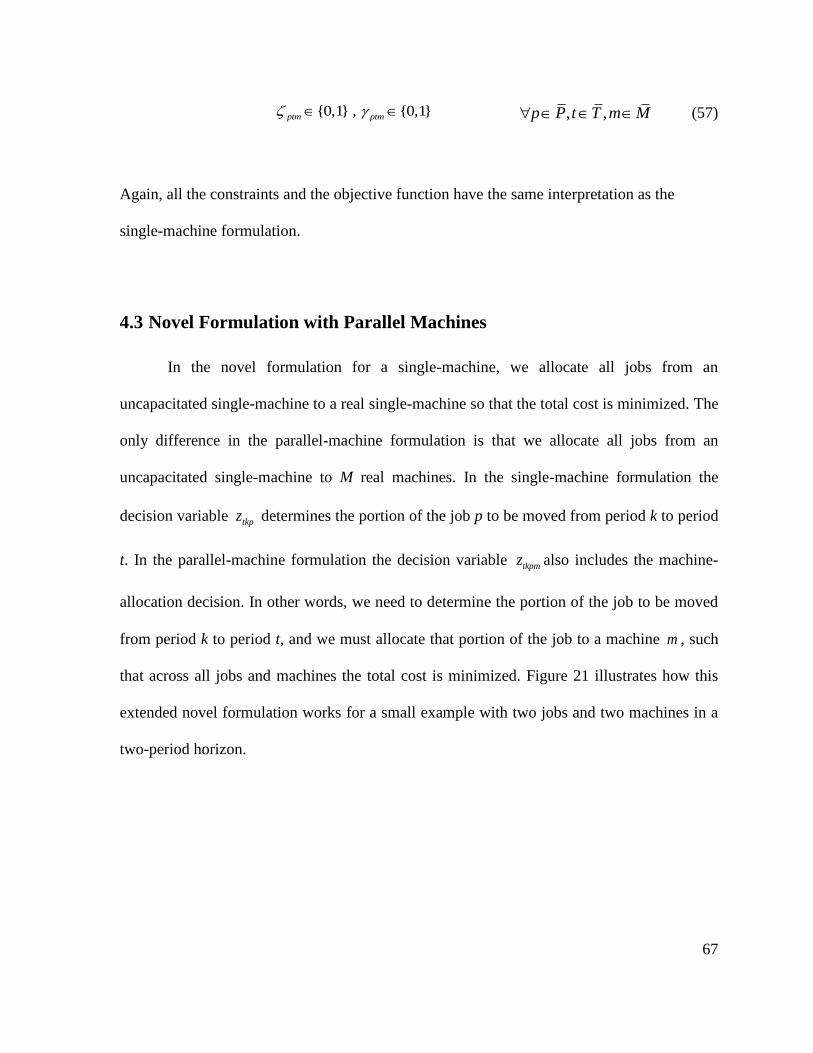
67

{0,1} , {0,1}ptm ptm , ,p P t T m M (57)

Again, all the constraints and the objective function have the same interpretation as the

single-machine formulation.

4.3 Novel Formulation with Parallel Machines

In the novel formulation for a single-machine, we allocate all jobs from an

uncapacitated single-machine to a real single-machine so that the total cost is minimized. The

only difference in the parallel-machine formulation is that we allocate all jobs from an

uncapacitated single-machine to M real machines. In the single-machine formulation the

decision variable tkpz determines the portion of the job p to be moved from period k to period

t. In the parallel-machine formulation the decision variable tkpmz also includes the machine-

allocation decision. In other words, we need to determine the portion of the job to be moved

from period k to period t, and we must allocate that portion of the job to a machine m , such

that across all jobs and machines the total cost is minimized. Figure 21 illustrates how this

extended novel formulation works for a small example with two jobs and two machines in a

two-period horizon.

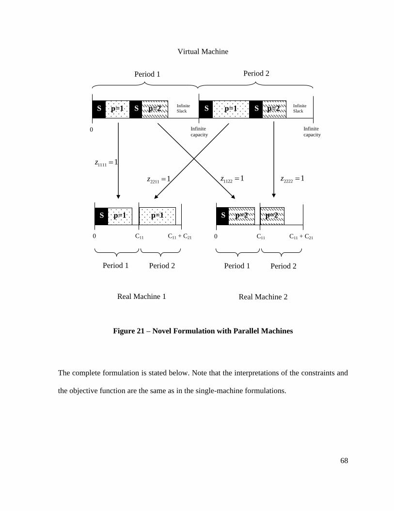
68

Figure 21 – Novel Formulation with Parallel Machines

The complete formulation is stated below. Note that the interpretations of the constraints and

the objective function are the same as in the single-machine formulations.

Real Machine 1 Real Machine 2

Virtual Machine

S S p=1 S p=2 S p=1 p=2

Period 1 Period 2

Infinite

capacity

Infinite

capacity

0

Infinite

Slack

Infinite

Slack

1111 1z

111 1z

1122 1z

111 1z

2222 1z

111 1z

Period 1 Period 2

C11

C11 + C21

0

Period 1 Period 2

C11

C11 + C21

0

2211 1z

111 1z

S p=1 p=1 S p=2 p=2

69

Minimize , 1,( ' )i s s

p pt p ptm p p t m

p Pt Tm M

c I c c

(58)

Subject to

, 1p t tkpm pk pt pt

k Tm M

I z d d I

,p P t T (59)

, 1,'u s s

p tkpm pk p ptm p p t m tm

p P k T

t z d t t C

,t T m M

(60)

' 'tkpm ptm

k T

z R

, ,p P t T m M (61)

1ptm

p P

,t T m M

(62)

, 1, , 1,2 ' ' 0ptm ptmp t m p t m

, ,p P t T m M

(63)

tkpm kp

t Tm M

z y

,p P k T

(64)

0 0

0 0, p m pm p pI I ,p P m M (65)

0 1tkpmz , , ,p P t T k T m M (66)

0ptI

,p P t T

(67)

{0,1} , ' {0,1}ptm ptm

, ,p P t T m M (68)

70

4.4 Computational Experiments

In this section, we first demonstrate the results from a two-machine experiment

without holding costs. We use the same data as in the single machine experiment in Chapters

2 and 3. The only difference is that the capacities are divided by two. In other words, we

assume that the parallel-machines are identical; thus, they have the same capacity. Following

this experiment we show the results from three-machine experiment. Again, we use the same

data and divide the capacities by three this time. The final experiment in this section is the

two-machine experiment with holding costs. In this experiment we use the Trigeiro et al. [11]

test bed that we used before.

The results from all these computational experiments confirm the conclusions we

made in previous chapter. The novel formulation outperforms the others in terms of

computation time and the gap. The classical formulation performs the worst among these

three formulations.

4.4.1 Two-Machine Experiment with Uniform Processing Times

In the first experiment we have two identical parallel-machines. We assume that

inventory holding costs are not significant. Since solving parallel-machine problems is much

harder as compared to single-machine problems, we do not expect to solve most of the

instances to optimality. Having that in mind, we set the gap tolerance level of CPLEX to 1%,

meaning that we terminate the process when the gap between the upper bound and the lower

bound is less than or equal to 1%. In other words, we assume that a solution with a gap of 1%

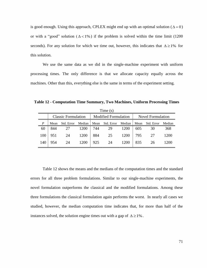
71

is good enough. Using this approach, CPLEX might end up with an optimal solution ( 0 )

or with a ―good‖ solution ( 1% ) if the problem is solved within the time limit (1200

seconds). For any solution for which we time out, however, this indicates that 1% for

this solution.

We use the same data as we did in the single-machine experiment with uniform

processing times. The only difference is that we allocate capacity equally across the

machines. Other than this, everything else is the same in terms of the experiment setting.

Table 12 - Computation Time Summary, Two Machines, Uniform Processing Times

Time (s)



60 844 27 1200 744 29 1200 605 30 368

100 951 24 1200 884 25 1200 795 27 1200

140 954 24 1200 925 24 1200 835 26 1200

Table 12 shows the means and the medians of the computation times and the standard

errors for all three problem formulations. Similar to our single-machine experiments, the

novel formulation outperforms the classical and the modified formulations. Among these

three formulations the classical formulation again performs the worst. In nearly all cases we

studied, however, the median computation time indicates that, for more than half of the

instances solved, the solution engine times out with a gap of 1% .

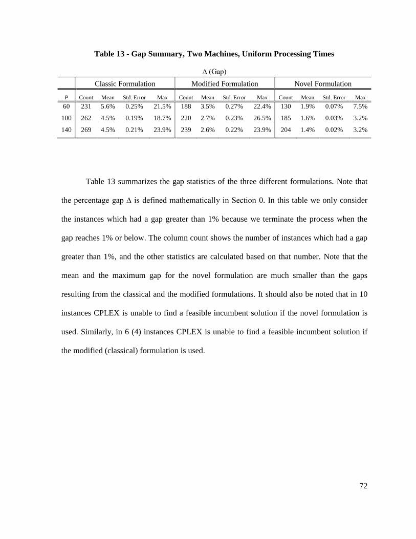
72

Table 13 - Gap Summary, Two Machines, Uniform Processing Times

∆ (Gap)



60 231 5.6% 0.25% 21.5% 188 3.5% 0.27% 22.4% 130 1.9% 0.07% 7.5%

100 262 4.5% 0.19% 18.7% 220 2.7% 0.23% 26.5% 185 1.6% 0.03% 3.2%

140 269 4.5% 0.21% 23.9% 239 2.6% 0.22% 23.9% 204 1.4% 0.02% 3.2%

Table 13 summarizes the gap statistics of the three different formulations. Note that

the percentage gap ∆ is defined mathematically in Section 0. In this table we only consider

the instances which had a gap greater than 1% because we terminate the process when the

gap reaches 1% or below. The column count shows the number of instances which had a gap

greater than 1%, and the other statistics are calculated based on that number. Note that the

mean and the maximum gap for the novel formulation are much smaller than the gaps

resulting from the classical and the modified formulations. It should also be noted that in 10

instances CPLEX is unable to find a feasible incumbent solution if the novel formulation is

used. Similarly, in 6 (4) instances CPLEX is unable to find a feasible incumbent solution if

the modified (classical) formulation is used.

73

Figure 22 - Average Computation Times vs. Problem size, Two Machines, Uniform

Distribution

Figure 22 shows the average computation times of different formulations with

different problem sizes. It should be noted that, as the instances get harder to solve, these

averages are being driven by the computation time limit more often. In other words, if we set

the computation time limit to 2000 seconds instead of 1200 seconds, then the averages would

be greater. The figure shows again that the average computation time required by the novel

formulation to solve the instances is less than the time required by the other two

formulations.

500

550

600

650

700

750

800

850

900

950

1000

60 100 140

Co

mp

uta

tio

n T

ime

(s)

Number of Products

classic

modified

novel

74

Figure 23 - Computation Time Performance, Two Machines, Uniform Distribution

(Cumulative)

Figure 24 - Gap Performance, Two Machines, Uniform Distribution (Cumulative)

15%

20%

25%

30%

35%

40%

45%

50%

0 100 200 300 400 500 600 700 800 900 1000 1100 1200

% o

f in

stan

ces

solv

ed

(w

ith

in 1

% g

ap)


classic

modified

novel

0%

10%

20%

30%

40%

50%

60%

70%

80%

90%

100%

0.0% 2.0% 4.0% 6.0% 8.0% 10.0%

% o

f in

stan

ces

solv

ed

∆ (Gap)

classic

modified

novel

75

Figure 23 shows that 48% of the instances can be solved to a gap of 1% using the

novel formulation within the computation time limit, while the modified and classical

formulations can solve only 37% and 28% of problem instances, respectively, to within a 1%

gap. (Recall that our computational experiment set contains 1080 instances in total.)

Figure 24 shows a cumulative graph of gap performance of our three formulations. It

can be easily seen that if the novel formulation is used, more than 90% of the instances can

be solved to a gap of 2% or less. If the modified formulation is used, 71% of the instances

can be solved to within 2%, and if the classical formulation is used only 48% of the instances

can be solved to within that gap tolerance. Similar to all the other graphs and statistics

presented in this research, this graph also confirms that the novel formulation outperforms

the other two formulations.

Figure 25 shows the gap distribution. (Please note that, to allow all differences to be

visible, the y-axis is in log-scale.) This histogram demonstrates that the range of the gaps is

much tighter if the novel formulation is used. That means we do not see ―bad surprises‖ like

in the modified and classical formulations. If we analyze the instances on the right tail of the

gap distributions of the classical and modified formulations, we see that those instances

mostly have high slackness and high density (see Appendix C). This result is consistent with

our lower bound analysis in Section 2.5

76

Figure 25 - Gap Distribution, Two-Machine Experiment, Uniform Processing Times

The experiment with two-machines and uniform processing times confirms our

conclusions from the previous chapters. It is obvious that the computation time and gap

performance of the novel formulation is superior to the modified and classical formulations.

4.4.2 Three-Machine Experiment with Uniform Processing Times

In this section we show the results of the three-machine experiment with uniform

processing times. Again, we take the same data that we used in the single-machine

experiment and divide the capacities by three this time. Otherwise, this experiment is

structured the same as the two-machine experiment.

1

10

100

1000

195

795

Nu

mb

er

of

Inst

ance

s

∆ (Gap)

classic

modified

novel

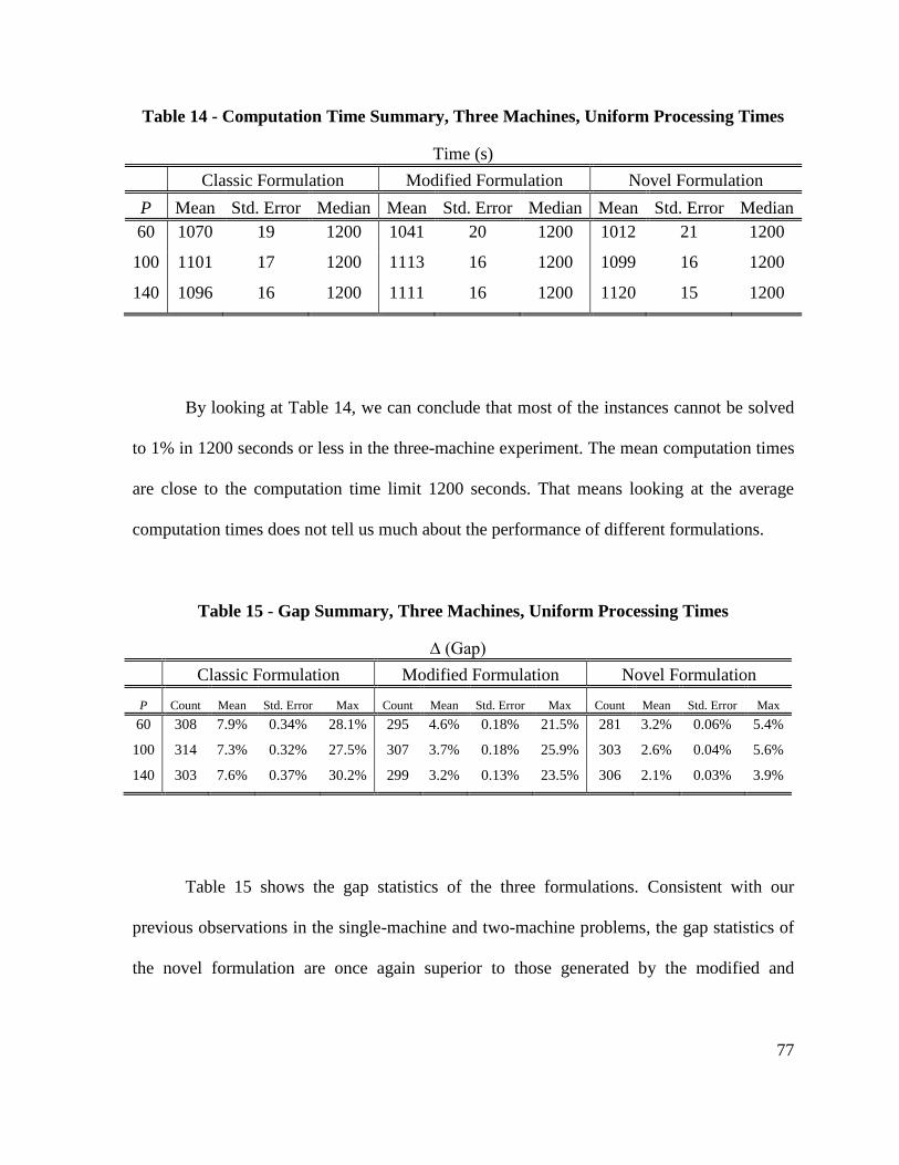
77

Table 14 - Computation Time Summary, Three Machines, Uniform Processing Times

Time (s)



60 1070 19 1200 1041 20 1200 1012 21 1200

100 1101 17 1200 1113 16 1200 1099 16 1200

140 1096 16 1200 1111 16 1200 1120 15 1200

By looking at Table 14, we can conclude that most of the instances cannot be solved

to 1% in 1200 seconds or less in the three-machine experiment. The mean computation times

are close to the computation time limit 1200 seconds. That means looking at the average

computation times does not tell us much about the performance of different formulations.

Table 15 - Gap Summary, Three Machines, Uniform Processing Times

∆ (Gap)



60 308 7.9% 0.34% 28.1% 295 4.6% 0.18% 21.5% 281 3.2% 0.06% 5.4%

100 314 7.3% 0.32% 27.5% 307 3.7% 0.18% 25.9% 303 2.6% 0.04% 5.6%

140 303 7.6% 0.37% 30.2% 299 3.2% 0.13% 23.5% 306 2.1% 0.03% 3.9%

Table 15 shows the gap statistics of the three formulations. Consistent with our

previous observations in the single-machine and two-machine problems, the gap statistics of

the novel formulation are once again superior to those generated by the modified and

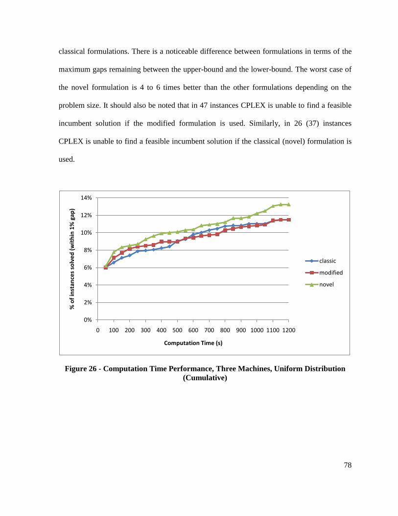
78

classical formulations. There is a noticeable difference between formulations in terms of the

maximum gaps remaining between the upper-bound and the lower-bound. The worst case of

the novel formulation is 4 to 6 times better than the other formulations depending on the

problem size. It should also be noted that in 47 instances CPLEX is unable to find a feasible

incumbent solution if the modified formulation is used. Similarly, in 26 (37) instances

CPLEX is unable to find a feasible incumbent solution if the classical (novel) formulation is

used.

Figure 26 - Computation Time Performance, Three Machines, Uniform Distribution

(Cumulative)

0%

2%

4%

6%

8%

10%

12%

14%

0 100 200 300 400 500 600 700 800 900 1000 1100 1200

% o

f in

stan

ces

solv

ed

(w

ith

in 1

% g

ap)


classic

modified

novel

79

Given what we know about the three-machine problem, however, Figure 26, which

shows the combined computation time and gap results, is not very informative. It merely

confirms that this problem is very hard to solve to near-optimality. Fewer than 14% of the

instances can be solved to within a 1% gap within the computation time limit regardless of

the chosen formulation. Figure 27 includes information from the instances that could not be

solved to 1% within the given time. The percentages of problem instances that can be solved

to within a 4% gap using the novel, modified and classical formulations are 92%, 72% and

48%, respectively. Again, the novel formulation outperforms the other two formulations in

terms of the solution quality, but none of the formulations performs particularly well in terms

of solving problems to within a 1 – 2% upper-lower bound gap.

Figure 27 - Gap Performance, Three Machines, Uniform Distribution (Cumulative)

0%

10%

20%

30%

40%

50%

60%

70%

80%

90%

100%

0.0% 2.0% 4.0% 6.0% 8.0% 10.0% 12.0% 14.0% 16.0% 18.0%

% o

f in

stan

ces

solv

ed

∆ (Gap)

classic

modified

novel

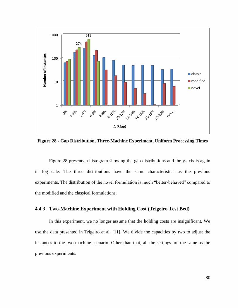
80

Figure 28 - Gap Distribution, Three-Machine Experiment, Uniform Processing Times

Figure 28 presents a histogram showing the gap distributions and the y-axis is again

in log-scale. The three distributions have the same characteristics as the previous

experiments. The distribution of the novel formulation is much ―better-behaved‖ compared to

the modified and the classical formulations.

4.4.3 Two-Machine Experiment with Holding Cost (Trigeiro Test Bed)

In this experiment, we no longer assume that the holding costs are insignificant. We

use the data presented in Trigeiro et al. [11]. We divide the capacities by two to adjust the

instances to the two-machine scenario. Other than that, all the settings are the same as the

previous experiments.

1

10

100

1000

274

613

Nu

mb

er

of

Inst

ance

s

∆ (Gap)

classic

modified

novel

81

The test bed has 751 instances in total with different product and period numbers. The

number of products ranges between 4 and 30 for the problem instances in this test bed, while

the number of periods ranges between 15 and 30. Different than the instances that we

generate in the experiments summarized above, these instances tend to have fewer products

but more periods.

Table 16 shows the basic computation time statistics in seconds. The mean

computation times and the medians for all three formulations show that we reach the time

limit, which is 1200 seconds, before being able to solve the problem.

Table 16 - Computation Time Summary, Two Machines, Trigeiro Test Bed

Time (s)


Mean 989 944 956

Std. Error 16 17 17

Median 1200 1200 1200

Table 17 below summarizes the gap statistics for the different formulations. The

count column gives the number of instances that could not be solved to optimality. All the

other statistics in this table are calculated based on those instances that could not be solved to

optimality. It should be noted that approximately 75% of the time we reach the computation

time limit before the gap between the upper-bound and the lower-bound is closed. Similar to

the previous experiments the mean gap is the lowest if the novel formulation is used and the

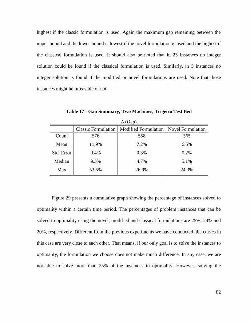
82

highest if the classic formulation is used. Again the maximum gap remaining between the

upper-bound and the lower-bound is lowest if the novel formulation is used and the highest if

the classical formulation is used. It should also be noted that in 23 instances no integer

solution could be found if the classical formulation is used. Similarly, in 5 instances no

integer solution is found if the modified or novel formulations are used. Note that those

instances might be infeasible or not.

Table 17 - Gap Summary, Two Machines, Trigeiro Test Bed

∆ (Gap)


Count 576 558 565

Mean 11.9% 7.2% 6.5%

Std. Error 0.4% 0.3% 0.2%

Median 9.3% 4.7% 5.1%

Max 53.5% 26.9% 24.3%

Figure 29 presents a cumulative graph showing the percentage of instances solved to

optimality within a certain time period. The percentages of problem instances that can be

solved to optimality using the novel, modified and classical formulations are 25%, 24% and

20%, respectively. Different from the previous experiments we have conducted, the curves in

this case are very close to each other. That means, if our only goal is to solve the instances to

optimality, the formulation we choose does not make much difference. In any case, we are

not able to solve more than 25% of the instances to optimality. However, solving the

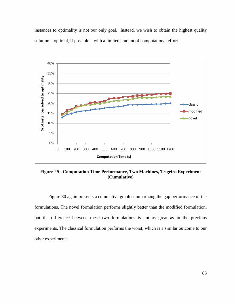
83

instances to optimality is not our only goal. Instead, we wish to obtain the highest quality

solution—optimal, if possible—with a limited amount of computational effort.

Figure 29 - Computation Time Performance, Two Machines, Trigeiro Experiment

(Cumulative)

Figure 30 again presents a cumulative graph summarizing the gap performance of the

formulations. The novel formulation performs slightly better than the modified formulation,

but the difference between these two formulations is not as great as in the previous

experiments. The classical formulation performs the worst, which is a similar outcome to our

other experiments.

0%

5%

10%

15%

20%

25%

30%

35%

40%

0 100 200 300 400 500 600 700 800 900 1000 1100 1200

% o

f in

stan

ces

solv

ed

to

op

tim

alit

y


classic

modified

novel

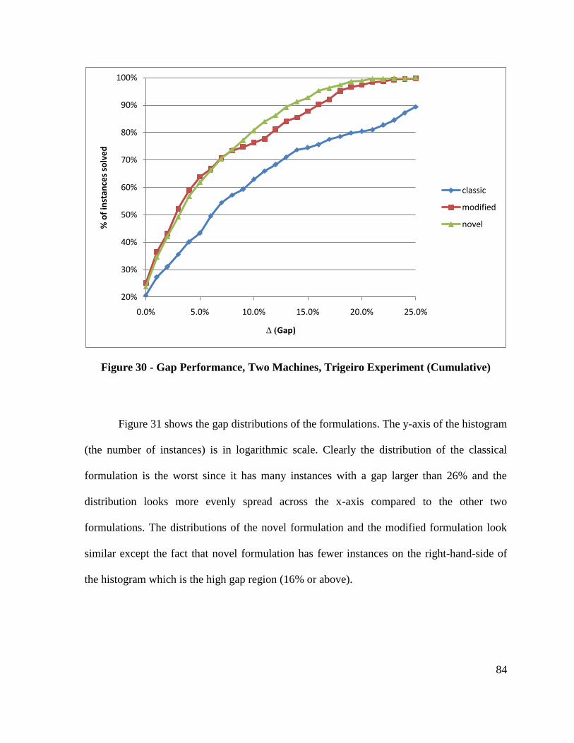
84

Figure 30 - Gap Performance, Two Machines, Trigeiro Experiment (Cumulative)

Figure 31 shows the gap distributions of the formulations. The y-axis of the histogram

(the number of instances) is in logarithmic scale. Clearly the distribution of the classical

formulation is the worst since it has many instances with a gap larger than 26% and the

distribution looks more evenly spread across the x-axis compared to the other two

formulations. The distributions of the novel formulation and the modified formulation look

similar except the fact that novel formulation has fewer instances on the right-hand-side of

the histogram which is the high gap region (16% or above).

20%

30%

40%

50%

60%

70%

80%

90%

100%

0.0% 5.0% 10.0% 15.0% 20.0% 25.0%

% o

f in

stan

ces

solv

ed

∆ (Gap)

classic

modified

novel

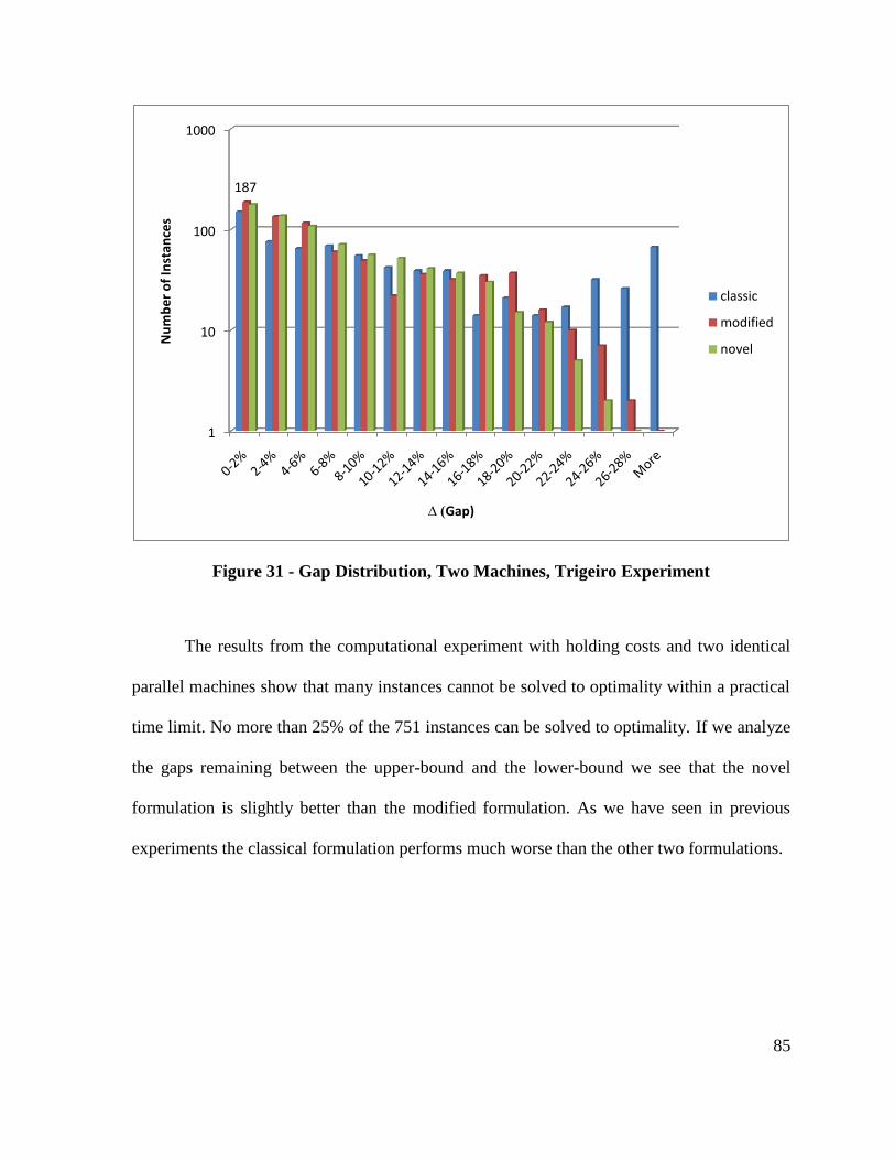
85

Figure 31 - Gap Distribution, Two Machines, Trigeiro Experiment

The results from the computational experiment with holding costs and two identical

parallel machines show that many instances cannot be solved to optimality within a practical

time limit. No more than 25% of the 751 instances can be solved to optimality. If we analyze

the gaps remaining between the upper-bound and the lower-bound we see that the novel

formulation is slightly better than the modified formulation. As we have seen in previous

experiments the classical formulation performs much worse than the other two formulations.

1

10

100

1000

187

Nu

mb

er

of

Inst

ance

s

∆ (Gap)

classic

modified

novel

86

4.5 Alternative Lower Bound

An important observation from our experiments above is that, as the branch and

bound process progresses, it becomes clear that the lower bound provided by the LP

relaxation, *

LPz , is not very tight and that this lower bound increases in only small increments

as the branch and bound process continues. At the same time, the solution process appears to

quickly settle on an incumbent solution (upper bound) that retains its incumbent status up to

the computation time limit. In this section, we use our MIP formulation to define an

alternative lower bound to the one provided by the branch and bound solution process in

CPLEX for the parallel-machine problem and we use this alternative lower bound as a more

accurate reference point to evaluate the quality of the MIP solutions.

The alternative lower bound for a given parallel-machine formulation can be

generated by relaxing its machine-dependent capacity constraints, effectively converting it

into a single-machine instance and then solving it as a single-machine problem. From

previous experiments we know that, particularly for our novel formulation, most of the

single-machine instances can be solved to optimality, or their solutions are very close to

optimal. Therefore, we use our novel formulation to generate the new lower bounds.

We convert a multiple-machine problem into a single-machine problem as follows:

Change the right-hand side of constraint (19) of the novel formulation (NMCLSP) to

be t tm

m M

C C

.

Replace constraint (21) in problem NMCLSP, 1pt

p P

, with pt

p P

M

.

87

The first change we make in the formulation can be interpreted as replacing the m

lower-capacity machines with a single high-capacity machine. This first change reduces the

total number of potential setup carry-overs. In order to include all the potential setup carry-

over savings, however, we also make the second change above. This modification can be

interpreted as follows: In a single-machine scenario, only a single setup can be carried over

from period t to period 1t but in a multiple-machine scenario, M setups can be carried over

from one period to the next.

By reformulating the parallel-machine problem as a single-machine problem as

shown above, we relax the problem by eliminating the allocation of jobs to machines. In

doing this, we also reduce the likelihood of an increase in overall setup cost that this

allocation entails. Because allocating the jobs to different machines will never decrease the

cost, then the optimal objective value of the single-machine relaxation of the parallel-

machine problem can never be higher than the optimal objective value of the parallel-

machine formulation. In other words, the optimal solution of this single-machine relaxation

of the parallel-machine problem gives a lower bound for the parallel-machine problem

because we solve a relaxed version of the problem.

We denote the lower bound generated by solving the single-machine relaxation of the

parallel-machine problem by SMz . We define the gap SMZ for each MIP formulation. The

best objective value of our MIP solution (classical, modified or novel formulation) to the

parallel-machine problem is denoted by PMz . As an alternative performance measure we

88

report the value of the deviation between the single-machine lower bound, SMz , and the MIP

objective PMz , as a percentage deviation, given by

100%.SM

PM SMZ

PM

z z

z

(69)

Let us call the gap reported by CPLEX &B B , which is defined as follows:

& 100%.PM LBB B

PM

z z

z

The term PMz defines the objective value of the current best integer solution (incumbent

solution) for the original parallel machine problem while *

LBz represents the objective value

of the LP relaxation optimal solution obtained for the current best node in the branch and

bound tree. Note that &B B is the value for

all the gaps we have reported up to this point.

Figure 32 and Figure 33 show the values of SMZ and &B B for the different

formulations of the two and three-machine problems. It is clear that the SMZ values are much

lower compared to the &B B values. That means that, overall, our alternative lower bound

SMz is a much tighter bound than the lower bound of the branch and bound tree *

LBz .

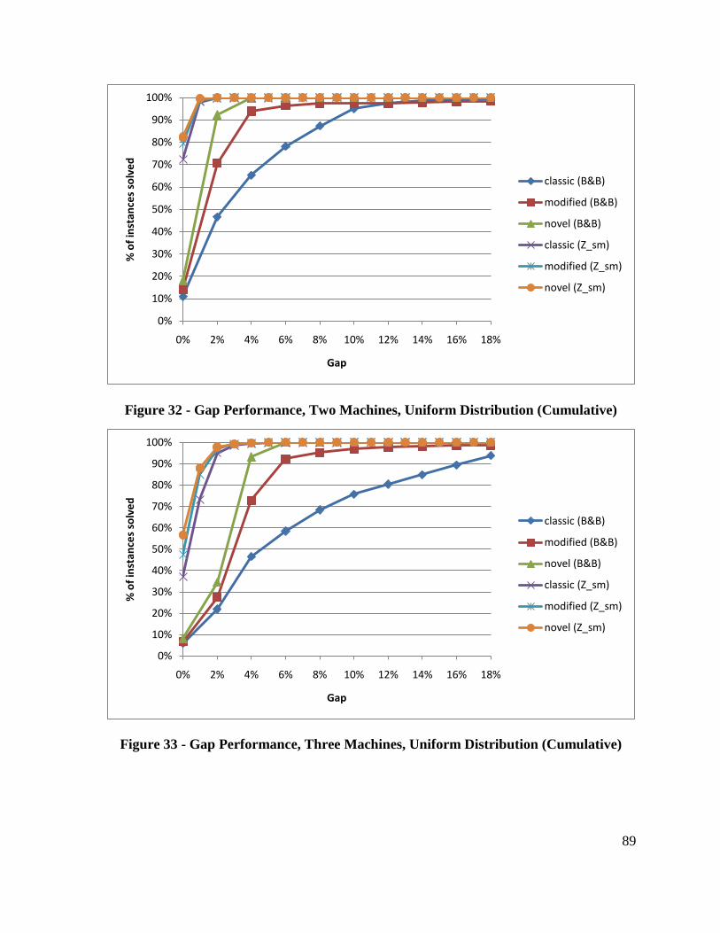
89


Figure 33 - Gap Performance, Three Machines, Uniform Distribution (Cumulative)

0%

10%

20%

30%

40%

50%

60%

70%

80%

90%

100%

0% 2% 4% 6% 8% 10% 12% 14% 16% 18%

% o

f in

stan

ces

solv

ed

Gap

classic (B&B)

modified (B&B)

novel (B&B)

classic (Z_sm)

modified (Z_sm)

novel (Z_sm)

0%

10%

20%

30%

40%

50%

60%

70%

80%

90%

100%

0% 2% 4% 6% 8% 10% 12% 14% 16% 18%

% o

f in

stan

ces

solv

ed

Gap

classic (B&B)

modified (B&B)

novel (B&B)

classic (Z_sm)

modified (Z_sm)

novel (Z_sm)

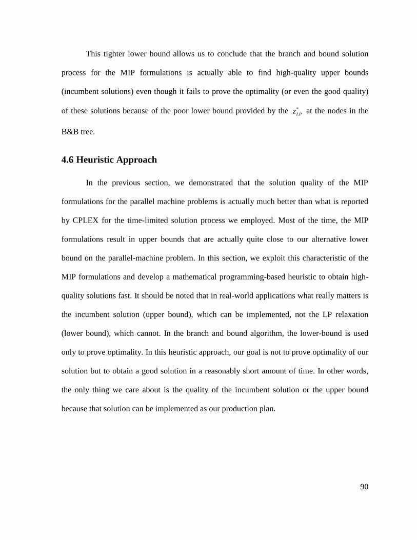
90

This tighter lower bound allows us to conclude that the branch and bound solution

process for the MIP formulations is actually able to find high-quality upper bounds

(incumbent solutions) even though it fails to prove the optimality (or even the good quality)

of these solutions because of the poor lower bound provided by the *

LPz at the nodes in the

B&B tree.

4.6 Heuristic Approach

In the previous section, we demonstrated that the solution quality of the MIP

formulations for the parallel machine problems is actually much better than what is reported

by CPLEX for the time-limited solution process we employed. Most of the time, the MIP

formulations result in upper bounds that are actually quite close to our alternative lower

bound on the parallel-machine problem. In this section, we exploit this characteristic of the

MIP formulations and develop a mathematical programming-based heuristic to obtain high-

quality solutions fast. It should be noted that in real-world applications what really matters is

the incumbent solution (upper bound), which can be implemented, not the LP relaxation

(lower bound), which cannot. In the branch and bound algorithm, the lower-bound is used

only to prove optimality. In this heuristic approach, our goal is not to prove optimality of our

solution but to obtain a good solution in a reasonably short amount of time. In other words,

the only thing we care about is the quality of the incumbent solution or the upper bound

because that solution can be implemented as our production plan.

91

4.6.1 Heuristic Algorithm

As mentioned before, the algorithm we develop in this section is based on single-

machine formulations of the parallel-machine problem and its single-machine sub-problems.

The algorithm has three main phases. In the first phase, the single-machine relaxation of the

parallel-machine problem is solved within a certain time limit. Based on the solution

obtained in phase one, products are allocated to the machines. This allocation process is the

second phase of the algorithm. After allocating all products to the machines, we solve M

independent single-machine problems as the final phase of the algorithm.

The algorithm includes two parameters to limit the computation time. The first

parameter 1t determines the maximum computation time allowed to solve the single-machine

relaxation of the parallel-machine problem in the first phase. The second parameter 2t limits

the computation time for solving each single-machine problem in the third phase of the

algorithm. In addition to those parameters, we keep track of two variables during the

allocation phase. These variables are defined as follows:

: Sum of processing times of all jobs allocated to machine in period rmg m r

: Sum of setup times of all jobs allocated to machine in period rmh m r

The steps of the algorithm are as follows:

Step 1: Try to solve the single-machine relaxation of the parallel-machine problem in 1t

seconds or less. If the optimal solution cannot be found in 1t seconds then save the

incumbent solution and go to Step 2.

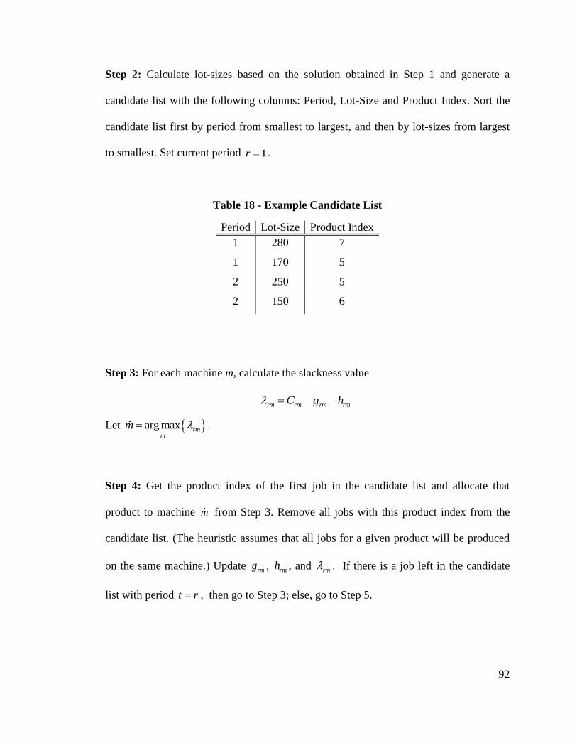
92

Step 2: Calculate lot-sizes based on the solution obtained in Step 1 and generate a

candidate list with the following columns: Period, Lot-Size and Product Index. Sort the

candidate list first by period from smallest to largest, and then by lot-sizes from largest

to smallest. Set current period 1r .

Table 18 - Example Candidate List

Period Lot-Size Product Index

1 280 7

1 170 5

2 250 5

2 150 6

Step 3: For each machine m, calculate the slackness value

rm rm rm rmC g h

Let arg max rmm

m .

Step 4: Get the product index of the first job in the candidate list and allocate that

product to machine m from Step 3. Remove all jobs with this product index from the

candidate list. (The heuristic assumes that all jobs for a given product will be produced

on the same machine.) Update rmg , rmh , and rm . If there is a job left in the candidate

list with period t r , then go to Step 3; else, go to Step 5.

93

Step 5: If the candidate list is empty go to Step 6; else, set 1r r and go to Step 3.

Step 6: Solve the resulting M independent single-machine problems, return their

solutions, and terminate.

Figure 34 presents the flowchart of the heuristic. Note that it is possible that Step 6

might not generate a feasible solution. Specifically, the job allocation to the machines that is

performed in Step 4 might lead to an infeasible single-machine instance in Step 6, even

though the original parallel-machine instance is feasible. In the future work section of the

next chapter, we discuss a suggested method to solve this issue. For now, we note that

infeasible solutions appear to be relatively rare in the computational experiments we describe

below. Such situations would require solution of the novel MIP formulation, using the best

incumbent solution that can be obtained from the time-constrained solution process.

94

Figure 34 – Flowchart of the Heuristic

START

Solve the single-machine relaxation in

t1 seconds

Generate and sort the candidate list based on the solution. Set current period

r=1.

Calculate the slackness values rm

, for

each machine m and let

arg maxrm

m

m

Get the product index of the first job in

the candidate list and allocate that

product to machine m

Remove all jobs with the same product

index from the candidate list. Update

rmg and

rmh

Is there any job left in the

candidate list

with period r?

Is r=T? Set 1r r

Solve the resulting M independent

single-machine problems, each in t2

seconds

END

YES

YES

NO

NO

95

4.6.2 Computational Experiments

In this section, we present the results of two computational experiments to assess our

heuristic approach. We choose the novel formulation as the underlying MIP formulation

because it has consistently outperformed the other two formulations in all experiments. In

both experiments in this section, we use the test bed of uniformly distributed processing

times that we generated earlier. The first experiment has two identical parallel machines and

the second has three identical parallel machines. In both experiments we set 1 50t seconds

and 2 20t seconds to keep the total computation time under 90 seconds. Other than the time

limits, all the settings are the same as the previous experiments.

Similar to the previous section, the lower bound generated by solving the single-

machine reformulation of the parallel-machine problem is denoted by SMz . Again, we use

this value as our benchmark in evaluating the performance of our heuristic solution to the

problem. The objective value of our heuristic solution to the parallel-machine problem is

denoted by H

PMz . Throughout the remainder of our analysis, we report the value of the

deviation between the single-machine lower bound, SMz , and the heuristic objective H

PMz , as

a percentage deviation, given by

100%.

H

PM SMPM SM

SM

z z

z

(70)

Before testing our heuristic procedure we solve the single-machine relaxations of the

parallel-machine problems with a time limit of 1200 seconds and save the resulting

96

objective values. We use these objective values later as a benchmark when we evaluate the

performance of the heuristic. In the rest of this chapter, we refer to those objective values

SMz . Note that the same problem is solved in Step 1 of the algorithm within the time limit

1t .

4.6.2.1 Two Machine Experiment

The first experiment we conduct to evaluate the performance of our heuristic is a two-

machine experiment with uniform processing times. Table 19 presents the percentage

deviation statistics from this experiment. The column ―feasible‖ shows the number of

instances where the solution of the heuristic is feasible and the column ―infeasible‖ shows the

number of instances where the solution of the heuristic is infeasible. It should be noted that

each row has 360 instances in total and our heuristic is able to find a feasible solution 95% of

the time. The mean and median percentage deviation statistics suggest that the heuristic

performs well overall, although there appear to be cases where it generates a relatively low-

quality solution (e.g., max deviation of greater than 10% for one of the 60-product problems).

Interestingly, the quality of the heuristic solution improves as the size of the problem

increases, in terms of the number of products.

Table 19 - Gap Summary of the Heuristic, Two Machines, Uniform Distribution

% Deviation from zSM

# of Products Feasible Infeasible Mean Std. Error Median Max

60 342 18 1.4% 0.07% 1.2% 10.7%

100 337 23 0.7% 0.04% 0.7% 4.0%

140 344 16 0.5% 0.03% 0.5% 4.2%

97

Table 20 shows the computation time statistics for the heuristic procedure. The values

in parentheses re-stated the statistics from the novel MIP formulation for the same test bed

(see Section 4.4.1). For example, the mean computation time of the heuristic to solve the

instances with 60 products is 18 seconds while the mean computation time for the novel MIP

formulation is 605 seconds. By looking at the mean and median statistics we can see that our

heuristic solves the problems in less than one minute, on average. As expected, as the

problem size increases, the required computation time for the heuristic also increases, but

compared to the computation times of the mixed integer formulations, the heuristic is very

fast. It should be also noted that the maximum required time is never more than two minutes,

as governed by the limits we set on 1t and 2t .

Table 20 - Computation Time Summary of the Heuristic, Two Machines, Uniform

Distribution

Time (s)

# of Products Mean Std. Error Median Max

60 18 (605) 1.2 (30) 6 (368) 103 (1200)

100 39 (795) 1.6 (27) 30 (1200) 105 (1200)

140 57 (835) 1.7 (26) 62 (1200) 118 (1200)

Figure 35 and Figure 36 demonstrate the percentage deviation from SMz as a function

of density and slackness, respectively. We see that as the slackness and density increase, the

percentage deviation tends to decrease. In addition to that, we also see that, as we indicated

above, as the problem size increases the percentage deviation decreases. This is mainly

98

because the denominator of expression (70) grows faster than its numerator as the problem

size gets bigger. Considering only the instances for which the heuristic could not provide a

feasible solution, we see that most of those infeasible instances have zero slackness. Note

that zero slackness means that the problem is very tight in terms of the capacity, so it is not

surprising that it is difficult to quickly find a good solution to these problems, and in those

cases, we must revert to solving the explicit MIP formulation.

Figure 35 - % Deviation from zSM vs. Density, Two Machines, Uniform Distribution

0.0%

0.5%

1.0%

1.5%

2.0%

0.5 0.7 0.9

Ave

rage

% D

evi

atio

n f

rom

zSM

Density

p=60

p=100

p=140

99

Figure 36 - % Deviation from zSM vs. Slackness, Two Machines, Uniform Distribution

Figure 37 and Figure 38 present the average heuristic computation times as a function

of density and slackness, respectively. As density increases the computation time increases.

This relationship makes sense because high density implies that the branch and bound trees

of the single-machine relaxation and the resulting M single-machine problems have more

nodes, and therefore more computation time is required to solve these sub-problems. In

Figure 38 we see that as slackness increases, the computation time decreases. This relation

also makes sense because the problem gets easier as slackness goes up, and therefore we

require less computation time.

0.0%

0.5%

1.0%

1.5%

2.0%

2.5%

0 0.25 0.5

Ave

rage

% D

evi

atio

n f

rom

zSM

Slackness

p=60

p=100

p=140

100

Figure 37 – Average Computation Time vs. Density, Two Machines, Uniform

Distribution

Figure 38 – Average Computation Time vs. Slackness, Two Machines, Uniform

Distribution

0

10

20

30

40

50

60

70

80

0.5 0.7 0.9

Ave

rage

Co

mp

uta

tio

n T

ime

(s)

Density

p=60

p=100

p=140

0

10

20

30

40

50

60

70

80

0 0.25 0.5

Ave

rage

Co

mp

uta

tio

n T

ime

(s)

Slackness

p=60

p=100

p=140

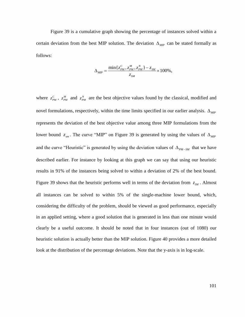
101

Figure 39 is a cumulative graph showing the percentage of instances solved within a

certain deviation from the best MIP solution. The deviation MIP can be stated formally as

follows:

min{ , , }100%,

C M N

PM PM PM SMMIP

SM

z z z z

z

where

C

PMz , M

PMz and N

PMz are the best objective values found by the classical, modified and

novel formulations, respectively, within the time limits specified in our earlier analysis. MIP

represents the deviation of the best objective value among three MIP formulations from the

lower bound smz . The curve ―MIP‖ on Figure 39 is generated by using the values of MIP

and the curve ―Heuristic‖ is generated by using the deviation values of PM SM that we have

described earlier. For instance by looking at this graph we can say that using our heuristic

results in 91% of the instances being solved to within a deviation of 2% of the best bound.

Figure 39 shows that the heuristic performs well in terms of the deviation from SMz . Almost

all instances can be solved to within 5% of the single-machine lower bound, which,

considering the difficulty of the problem, should be viewed as good performance, especially

in an applied setting, where a good solution that is generated in less than one minute would

clearly be a useful outcome. It should be noted that in four instances (out of 1080) our

heuristic solution is actually better than the MIP solution. Figure 40 provides a more detailed

look at the distribution of the percentage deviations. Note that the y-axis is in log-scale.

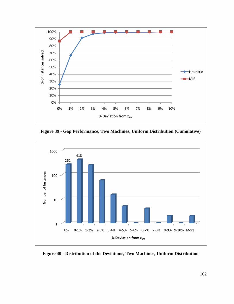
102


Figure 40 - Distribution of the Deviations, Two Machines, Uniform Distribution

0%

10%

20%

30%

40%

50%

60%

70%

80%

90%

100%

0% 1% 2% 3% 4% 5% 6% 7% 8% 9% 10%

% o

f in

stan

ces

solv

ed


Heuristic

MIP

1

10

100

1000

0% 0-1% 1-2% 2-3% 3-4% 4-5% 5-6% 6-7% 7-8% 8-9% 9-10% More

262

418

Nu

mb

er

of

Inst

ance

s


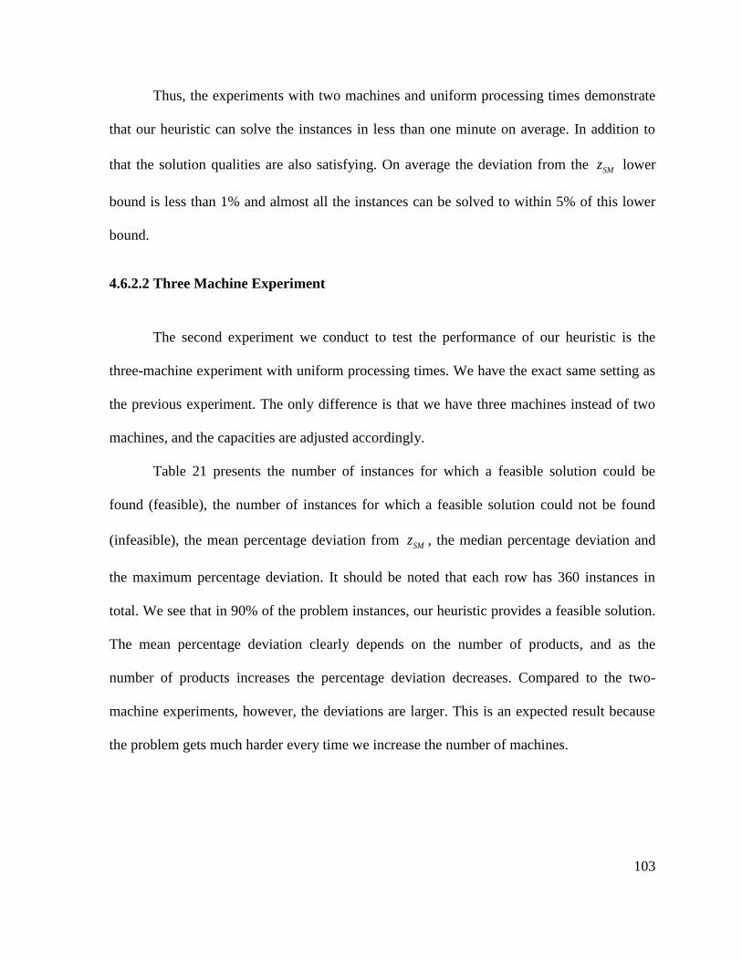
103

Thus, the experiments with two machines and uniform processing times demonstrate

that our heuristic can solve the instances in less than one minute on average. In addition to

that the solution qualities are also satisfying. On average the deviation from the SMz lower

bound is less than 1% and almost all the instances can be solved to within 5% of this lower

bound.

4.6.2.2 Three Machine Experiment

The second experiment we conduct to test the performance of our heuristic is the

three-machine experiment with uniform processing times. We have the exact same setting as

the previous experiment. The only difference is that we have three machines instead of two

machines, and the capacities are adjusted accordingly.

Table 21 presents the number of instances for which a feasible solution could be

found (feasible), the number of instances for which a feasible solution could not be found

(infeasible), the mean percentage deviation from SMz , the median percentage deviation and

the maximum percentage deviation. It should be noted that each row has 360 instances in

total. We see that in 90% of the problem instances, our heuristic provides a feasible solution.

The mean percentage deviation clearly depends on the number of products, and as the

number of products increases the percentage deviation decreases. Compared to the two-

machine experiments, however, the deviations are larger. This is an expected result because

the problem gets much harder every time we increase the number of machines.

104

Table 21 - Gap Summary of the Heuristic, Three Machines, Uniform Distribution


# of Products Feasible Infeasible Mean Std. Error Median Max

60 330 30 2.6% 0.10% 2.3% 10.4%

100 321 39 1.5% 0.07% 1.2% 10.9%

140 334 26 1.1% 0.05% 0.9% 5.4%

Table 22 presents the basic statistics for the computation times. Again, the values in

parentheses represent the computation time statistics of the novel formulation for the same

test bed. The values for the heuristic are very close to the results of the two-machine

experiments, while the difference between the heuristic and the novel formulation becomes

greater. This suggests that the heuristic is stable in terms of the computation time, governed,

of course, by the computation time limits 1t and 2t .

Table 22 - Computation Time Summary of the Heuristic, Three Machines, Uniform

Distribution

Time (s)

# of Products Mean Std. Error Median Max

60 17 (1012) 1 (21) 5 (1200) 104 (1200)

100 35 (1099) 2 (16) 20 (1200) 130 (1200)

140 53 (1120) 2 (15) 60 (1200) 134 (1200)

Figure 41 and Figure 42 show the change in average percentage deviation with

respect to density and slackness. As we observed earlier the percentage deviation tends to

decrease as density and/or slackness increase.

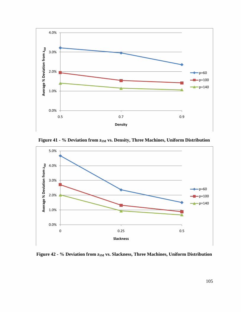
105

Figure 41 - % Deviation from zSM vs. Density, Three Machines, Uniform Distribution

Figure 42 - % Deviation from zSM vs. Slackness, Three Machines, Uniform Distribution

0.0%

1.0%

2.0%

3.0%

4.0%

0.5 0.7 0.9

Ave

rage

% D

evi

atio

n f

rom

zSM

Density

p=60

p=100

p=140

0.0%

1.0%

2.0%

3.0%

4.0%

5.0%

0 0.25 0.5

Ave

rage

% D

evi

atio

n f

rom

zSM

Slackness

p=60

p=100

p=140

106

Similarly, Figure 43 and Figure 44 show the change in computation time as a function

of density and slackness. Again, we observe the same relationship as we saw in the two-

machine experiment. The average computation time increases as density increases, and it

decreases as slackness increases. The reasoning behind this relationship is the same as in the

two-machine experiment.

Figure 43 – Average Computation Time vs. Density, Three Machines, Uniform

Distribution

0

10

20

30

40

50

60

70

80

0.5 0.7 0.9

Ave

rage

Co

mp

uta

tio

n T

ime

(s)

Density

p=60

p=100

p=140

107

Figure 44 - Average Computation Time vs. Slackness, Three Machines, Uniform

Distribution

Figure 45 and Figure 46 present the deviation characteristics in more detail. We use

the MIP and PM SM values as we did in the two-machine experiment. It is clear that the

performance of the heuristic is affected negatively by the increase in the number of

machines. But the performance is still reasonable. Almost all of the problem instances can be

solved to within 6% deviation from SMz . It should be noted that, in this case, in seven

instances (out of 1080) our heuristic solution is better than the MIP solution. Note that the y-

axis of the histogram is in log-scale.

0

10

20

30

40

50

60

70

80

0 0.25 0.5

Ave

rage

Co

mp

uta

tio

nal

Tim

e (

s)

Slackness

p=60

p=100

p=140

108

Figure 45 – Gap Performance, Three Machines, Uniform Distribution (Cumulative)

Figure 46 - Distribution of the Deviations, Three Machines, Uniform Distribution

0%

10%

20%

30%

40%

50%

60%

70%

80%

90%

100%

0% 1% 2% 3% 4% 5% 6% 7% 8% 9% 10%

% o

f in

stan

ces

solv

ed


Heuristic

MIP

1

10

100

1000

0% 0-1% 1-2% 2-3% 3-4% 4-5% 5-6% 6-7% 7-8% 8-9% 9-10% More

286 331

Nu

mb

er

of

Inst

ance

s


109

The computational experiment with three-machines and uniform processing times

showed that our heuristic is able to find a feasible solution 90% of the time. The average

deviation from the best possible objective value is 2%, and 98% of feasible solutions are

within a 6% deviation from the lower bound provided by the single-machine reformulation.

Considering the solution quality and the average computation time, it can be said that the

performance of the heuristic is satisfying.

In this section, we developed a mathematical programming-based heuristic to attempt

to generate high-quality solutions in significantly less time than the 1200-second

computational limit on the B&B process used to solve the MIP formulations of the parallel-

machine problem. Our heuristic can solve two-machine (three-machine) instances to within

0.9% (1.8%) of the single-machine formulation bound, on average, in an average

computation time of less than one minute. However the heuristic fails to find a feasible

solution for two-machine (three-machine) problems 5% (10%) of the time, and results in a

solution gap to the lower bound of 5% or higher in some cases. In future work, the heuristic

should be improved to address this issue. One possible approach to improving the algorithm

is to try different allocations to the machines after realizing that the initial allocation leads to

an infeasible solution. The current version of the heuristic tries only one allocation and if it

leads to an infeasible solution it stops. Further improvements are discussed in the future work

section of this study.

110

4.7 Conclusion

In this chapter we extended all three formulations to solve single-stage, parallel-

machine problems. We assume that machines have the same function, so a job can be

allocated to any machine. We also assume that the processing times of jobs are the same for

different machines. Our computational experiments with uniformly distributed processing

times and no holding costs showed that the novel model outperforms the classical and

modified formulations. As expected, as the number of machines increases, the likelihood that

the problem can be solved to a reasonably small lower/upper bound gap with a reasonable

level of computational effort decreases dramatically. We also conducted an experiment with

holding costs using Trigeiro et al. [11] test bed. The novel formulation and modified

formulation perform similarly on this test bed, with the novel formulation demonstrating a

slight edge in the lower bound-upper bound gap ∆, while the modified formulation solves

seven more (of 751) problems to optimality. In all parallel-machine experiments, the classical

formulation performed the worst as observed before.

We also used the MIP formulation to motivate the development of a single-machine,

relaxed formulation of the problem that results in a tighter lower bound on the parallel-

machine problem. Using this tighter lower bound, we observed that the quality of the

solutions that result from a time-restricted branch and bound on the MIP formulations is

actually quite good. To exploit the fact that single-machine problems can be solved relatively

quickly, we used our relaxed formulation to develop a mathematical programming-based

heuristic. The heuristic we introduce in this chapter is based on our novel formulation and

generates good solutions—on average, to within 0.9% (1.8%) of our two-machine (three-

111

machine) lower bound—in less than one minute, on average, across our computational

experiments.

112

CHAPTER 5

5 CONCLUSION AND FUTURE WORK

We first summarize our findings and then discuss potential extensions of our work.

5.1 Summary of Findings

In this study we developed a novel formulation to solve capacitated lot-sizing

problems (CLSP’s) with setup carry-overs. We showed that the classical and modified

formulations and our novel formulation can be converted to each other by using a variable

redefinition technique. Although the novel formulation might have more continuous

variables depending on the length of the planning horizon, our extensive computational

experiments showed that the novel formulation is superior to the other two formulations in

terms of computation time, measured as CPU time, and percentage gap ∆, which is defined

113

formally in Section 0. We also observed that the classical formulation performs by far the

worst among these three formulations on these measures.

We first compared the classical formulation with the modified formulation and

showed that the branch and bound tree of the second is much more compact than the first.

Then we compared the modified formulation with the novel formulation. We know that these

two formulations have the same integer variable characteristics; thus, they have a similar

branch and bound tree structure. We demonstrated, however, that the reason for the

performance difference between these two formulations is the quality of their lower-bounds

(LP relaxation). The quality of the lower-bound is driven by the ―big R‖ constraint, where the

novel formulation produces much tighter lower-bounds due to its small value of ―big R‖

equal to the total number of periods T. The lower-bound characteristics of the formulations

have the following implications.

- Our experiments show that, keeping all else the same, as slackness increases the

computation time and resulting solution gap both increase for the modified

formulation as compared to the novel formulation. (See Appendix C.)


regarding the effect of a shorter planning horizon: Keeping everything else the same,


driven by the length of the planning horizon for the novel formulation compared to

the modified formulation.

114


regarding the effect of a lower density: Keeping everything else the same,


driven by the lower density for the modified formulation compared to the novel

formulation.

The different computational experiments without holding costs, with holding costs,

with a single machine and with identical parallel machines have produced consistently the

same result. In all those experiments we observed that the novel formulation outperforms the

other two formulations and the modified formulation is better than the classical formulation.

The heuristic that we developed in the last chapter solves instances with 2m or

3m machines in less than one minute, on average. For the 5% (10%) of the two-machine

(three-machine) instances no feasible solution can be found. The computational tests with

uniformly distributed processing times showed that our mathematical programming based

heuristic is able to solve more than 99% (98%) of the two-machine (three-machine)

instances, for which it could find a feasible solution, to within 5% (6%) of the single-

machine lower bound.

5.2 Future Work

As to future work, we have two potential extension opportunities. The first one is to

extend the novel formulation for multiple-level systems. For instance, if the output of the first

machine is the input for the second machine then we call that system a two-stage system.

Since the novel formulation has an underlying fixed charged network flow structure, we

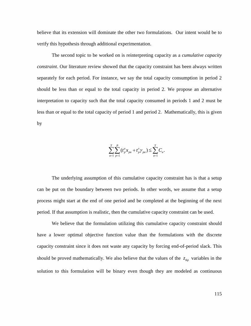
115

believe that its extension will dominate the other two formulations. Our intent would be to

verify this hypothesis through additional experimentation.

The second topic to be worked on is reinterpreting capacity as a cumulative capacity

constraint. Our literature review showed that the capacity constraint has been always written

separately for each period. For instance, we say the total capacity consumption in period 2

should be less than or equal to the total capacity in period 2. We propose an alternative

interpretation to capacity such that the total capacity consumed in periods 1 and 2 must be

less than or equal to the total capacity of period 1 and period 2. Mathematically, this is given

by

1 1 1

( ) .T P T

u s

p pa p pa a

a p a

t x t C

The underlying assumption of this cumulative capacity constraint has is that a setup

can be put on the boundary between two periods. In other words, we assume that a setup

process might start at the end of one period and be completed at the beginning of the next

period. If that assumption is realistic, then the cumulative capacity constraint can be used.

We believe that the formulation utilizing this cumulative capacity constraint should

have a lower optimal objective function value than the formulations with the discrete

capacity constraint since it does not waste any capacity by forcing end-of-period slack. This

should be proved mathematically. We also believe that the values of the tkpz variables in the

solution to this formulation will be binary even though they are modeled as continuous

116

variables between 0 and 1. If this is true, it means we should be able to further exploit the

underlying network flow structure in solving the novel formulation.

In addition to the extensions above, we believe that the heuristic that we introduced in

Chapter 4 can be extended. The heuristic, as it is, occasionally fails to generate feasible

solutions, especially when density is high and slackness is low. A possible way to solve

that problem is adding another step to the algorithm, in which we try pair-wise switches to

find a feasible solution within time limit 3t . The critical point here is how to decide which

jobs to choose for pair-wise switches. We have observed from our computational

experiments that most of the time infeasibility is caused by the jobs in first two periods, so it

would be wise to focus on the jobs in these periods. Total randomization is one option for

choosing jobs to switch in these periods, and other options should be explored further by

conducting computational tests. Other than the feasibility issue, the solution quality for the

low slackness instances should be improved further. One way to do it is to include a pre-

processing phase and detect the low slackness instances before the solution process start.

After that we can try different allocation algorithms for those ―special instances‖ and report

the best solution.

117

REFERENCES

[1] A. Allahverdi, J. N. D. Gupta, and T. Aldowaisan, ―A review of scheduling research

involving setup considerations,‖ Omega, Int. J. Mgmt Sci., vol. 27, no. 2, pp. 219-239,

Apr. 1999.

[2] A. Allahverdi, C. Ng, T. Cheng, and M. Kovalyov, ―A survey of scheduling problems

with setup times or costs,‖ European Journal of Operational Research, vol. 187, no. 3,

pp. 985-1032, Jun. 2008.

[3] I. Ovacik and R. Uzsoy, Decomposition methods for complex factory scheduling

problems. Boston: Kluwer Academic Publishers, 1997.

[4] C. N. Potts and M. Y. Kovalyov, ―Scheduling with batching: A review,‖ European

Journal of Operational Research, vol. 120, no. 2, pp. 228-249, Jan. 2000.

[5] K. R. Baker, ―Heuristic procedures for scheduling job families with setups and due

dates,‖ Naval Research Logistics, vol. 46, no. 8, pp. 978-991, Dec. 1999.

[6] R. Uzsoy and J. D. Velasquez, ―Heuristics for minimizing maximum lateness on a

single machine with family-dependent set-up times,‖ Computers & Operations

Research, vol. 35, no. 6, pp. 2018-2033, Jun. 2008.

[7] J. Bruno and P. Downey, ―Complexity of task sequencing with deadlines, set-up times

and changeover costs,‖ SIAM Journal on Computing, vol. 7, no. 4, pp. 393-404, 1978.

[8] A. T. Unal and A. S. Kiran, ―Batch sequencing,‖ IIE Transactions, vol. 24, no. 4, pp.

73-83, Sep. 1992.

[9] W. C. Driscoll and H. Emmons, ―Scheduling production on one machine with

changeover costs,‖ IIE Transactions, vol. 9, no. 4, pp. 388-395, Dec. 1977.

[10] C. L. Monma and C. N. Potts, ―On the complexity of scheduling with batch setup

times,‖ Operations Research, vol. 37, no. 5, pp. 798-804, 1989.

[11] W. W. Trigeiro, L. J. Thomas, and J. O. McClain, ―Capacitated Lot Sizing with Setup

Times,‖ Management Science, vol. 35, no. 3, pp. 353-366, Mar. 1989.

[12] P. J. Billington, J. O. Mcclain, and J. L. Thomas, ―Mathematical Programming

Approaches to Capacity-Constrained MRP Systems : Review, Formulation and

Problem Reduction,‖ Management Science, vol. 29, no. 10, pp. 1126-1141, 1983.

118

[13] L. P. Ritzman and H. C. Bahl, ―An Integrated Formulation for Master Scheduling , Lot

Sizing and Capacity Requirements Planning,‖ Journal of the Operational Research

Society, vol. 35, no. 5, pp. 389- 399, 1984.

[14] G. R. Bitran and H. H. Yanasse, ―Computational Complexity of the Capacitated Lot

Size Problem,‖ Management Science, vol. 28, no. 10, pp. 1174-1186, Oct. 1982.

[15] J. Maes, J. O. Mcclain, and V. L. N. Wassenhove, ―Multilevel capacitated lotsizing

complexity and LP-based heuristics,‖ European Journal Of Operational Research,

vol. 53, pp. 131-148, 1991.

[16] C. R. Sox and Y. Gao, ―The capacitated lot sizing problem with setup carry-over,‖ IIE

Transactions, vol. 31, pp. 173-181, 1999.

[17] K. Haase, ―Capacitated Lot-Sizing with Linked Production Quantities of Adjacent

Periods,‖ in Beyond manufacturing resource planning (MRP II)—advanced

formulations and methods for production planning, Berlin: Springer, 1998, pp. 127-

146.

[18] C. Dillenberger, ―On practical resource allocation for production planning and

scheduling with period overlapping setups,‖ European Journal of Operational

Research, vol. 75, no. 2, pp. 275-286, Jun. 1994.

[19] M. Gopalakrishnan, D. M. Miller, and C. P. Schmidt, ―A framework for

formulationling setup carryover in the capacitated lot sizing problem,‖ International

Journal of Production Research, vol. 33, no. 7, pp. 1973-1988, Jul. 1995.

[20] D. Quadt and H. Kuhn, ―Capacitated lot-sizing with extensions: a review,‖ 4or, vol. 6,

no. 1, pp. 61-83, Oct. 2007.

[21] B. Karimi, ―The capacitated lot sizing problem: a review of formulations and

algorithms,‖ Omega, vol. 31, no. 5, pp. 365-378, Oct. 2003.

[22] C. N. Potts and V. L. N. Wassenhove, ―Integrating scheduling with batching and lot-

Sizing: A review of algorithms and complexity,‖ Journal of the Operational Research

Society, vol. 43, no. 5, pp. 395-406, May 1992.

[23] H. Meyr, ―Simultaneous lotsizing and scheduling on parallel machines,‖ European

Journal of Operational Research, vol. 139, no. 2, pp. 277-292, Jun. 2002.

[24] G. D. Eppen and R. K. Martin, ―Solving Multi-Item Capacitated Lot-Sizing Problems

Using Variable Redefinition,‖ Operations Research, vol. 35, no. 6, pp. 832-848, 1987.

119

APPENDICES

120

Appendix A

In this appendix, we first show that the classical, restricted formulation is equivalent

to the modified formulation. Then we demonstrate that the modified formulation and the

novel formulation are equivalent. In each step, we apply a linear transformation to the

decision variables and apply that linear transformation to all constraints including the

corresponding variable. After the linear transformation, if all constraints are equivalent, we

conclude that the formulations are equivalent to each other. It is important that no feasible

solution is lost and no new feasible solution is generated during the linear transformation.

After showing that all these are true, we conclude that ―left-shifts‖ done by the novel

formulation (starting from the lot-for-lot plan) leads to an optimal solution, if there is any.

Proposition 1: The modified formulation (MCLSP) is equivalent to the restricted

formulation (CRCLSP).

Proof: Apply the following linear transformation to the variable 'pt :

, 1'pt pt p t

If we can show that these two formulations can be converted to each other by

applying the linear transformation above then we can say that these two formulations are

equivalent.

After comparing the two formulations we see that constraints (4), (7), (8), (9) and

(12) are common in both formulations and do not include the variable pt or 'pt . It does not

require much effort to show that the objective function (17) can easily be converted to the

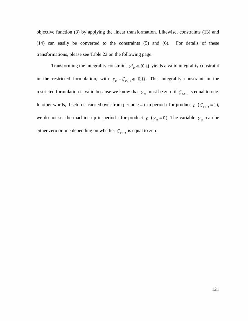
121

objective function (3) by applying the linear transformation. Likewise, constraints (13) and

(14) can easily be converted to the constraints (5) and (6). For details of these

transformations, please see Table 23 on the following page.

Transforming the integrality constraint ' {0,1}pt yields a valid integrality constraint

in the restricted formulation, with , 1 {0,1}pt p t . This integrality constraint in the

restricted formulation is valid because we know that pt must be zero if

, 1p t is equal to one.

In other words, if setup is carried over from period 1t to period t for product p (, 1 1p t ),

we do not set the machine up in period t for product p ( 0pt ). The variable pt can be

either zero or one depending on whether , 1p t

is equal to zero.

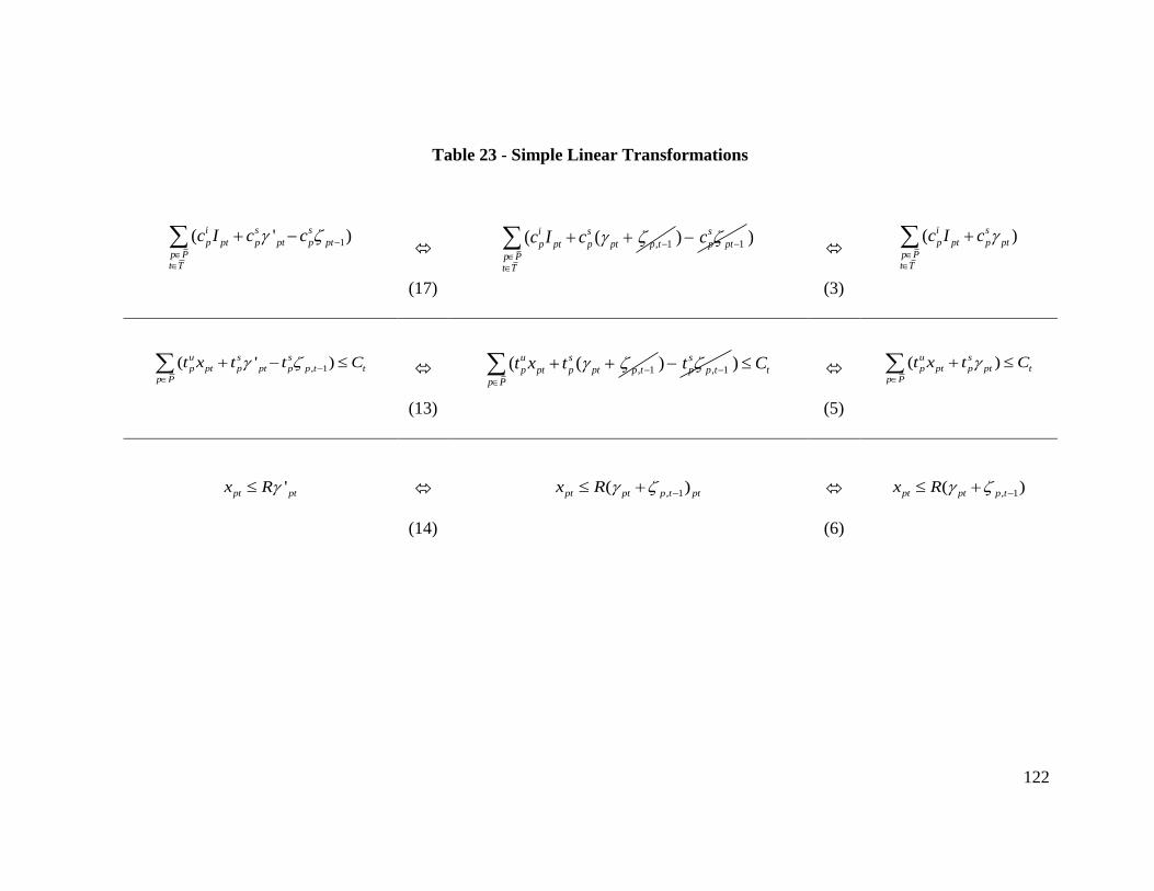
122

Table 23 - Simple Linear Transformations

1( ' )i s s

p pt p pt p pt

p Pt T

c I c c

(17)

, 1( (i s

p pt p pt p t

p Pt T

c I c

1) s

p ptc )

(3)

( )i s

p pt p pt

p Pt T

c I c

, 1( ' )u s s

p pt p pt p p t t

p P

t x t t C

(13)

, 1( (u s

p pt p pt p tt x t , 1) s

p p tt ) t

p P

C

(5)

( )u s

p pt p pt t

p P

t x t C

'pt ptx R

(14)

, 1( )pt pt p t ptx R

(6)

, 1( )pt pt p tx R

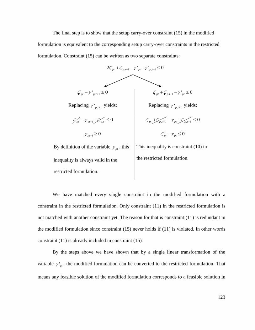
123

The final step is to show that the setup carry-over constraint (15) in the modified

formulation is equivalent to the corresponding setup carry-over constraints in the restricted

formulation. Constraint (15) can be written as two separate constraints:

, 1 , 12 ' ' 0pt p t pt p t

, 1' 0pt p t , 1 ' 0pt p t pt

Replacing , 1'p t

yields: Replacing , 1'p t

yields:

pt 1 ,pt p t 0 , 1pt p t , 1pt p t 0

1 0pt 0pt pt

By definition of the variable pt , this

inequality is always valid in the

restricted formulation.

This inequality is constraint (10) in

the restricted formulation.

We have matched every single constraint in the modified formulation with a

constraint in the restricted formulation. Only constraint (11) in the restricted formulation is

not matched with another constraint yet. The reason for that is constraint (11) is redundant in

the modified formulation since constraint (15) never holds if (11) is violated. In other words

constraint (11) is already included in constraint (15).

By the steps above we have shown that by a single linear transformation of the

variable 'pt , the modified formulation can be converted to the restricted formulation. That

means any feasible solution of the modified formulation corresponds to a feasible solution in

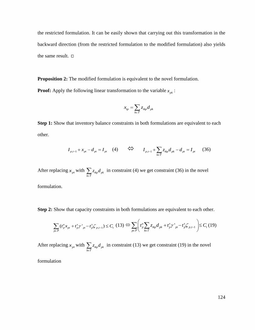
124

the restricted formulation. It can be easily shown that carrying out this transformation in the

backward direction (from the restricted formulation to the modified formulation) also yields

the same result.

Proposition 2: The modified formulation is equivalent to the novel formulation.

Proof: Apply the following linear transformation to the variablepkx :

tp tkp pk

k T

x z d

Step 1: Show that inventory balance constraints in both formulations are equivalent to each

other.

, 1p t pt pt ptI x d I (4) , 1p t tkp pk pt pt

k T

I z d d I

(36)

After replacingptx with

tkp pk

k T

z d

in constraint (4) we get constraint (36) in the novel

formulation.

Step 2: Show that capacity constraints in both formulations are equivalent to each other.

, 1( ' )u s s

p pt p pt p p t t

p P

t x t t C

(13) , 1'u s s

p tkp pk p pt p p t t

p P k T

t z d t t C

(19)

After replacingptx with

tkp pk

k T

z d

in constraint (13) we get constraint (19) in the novel

formulation

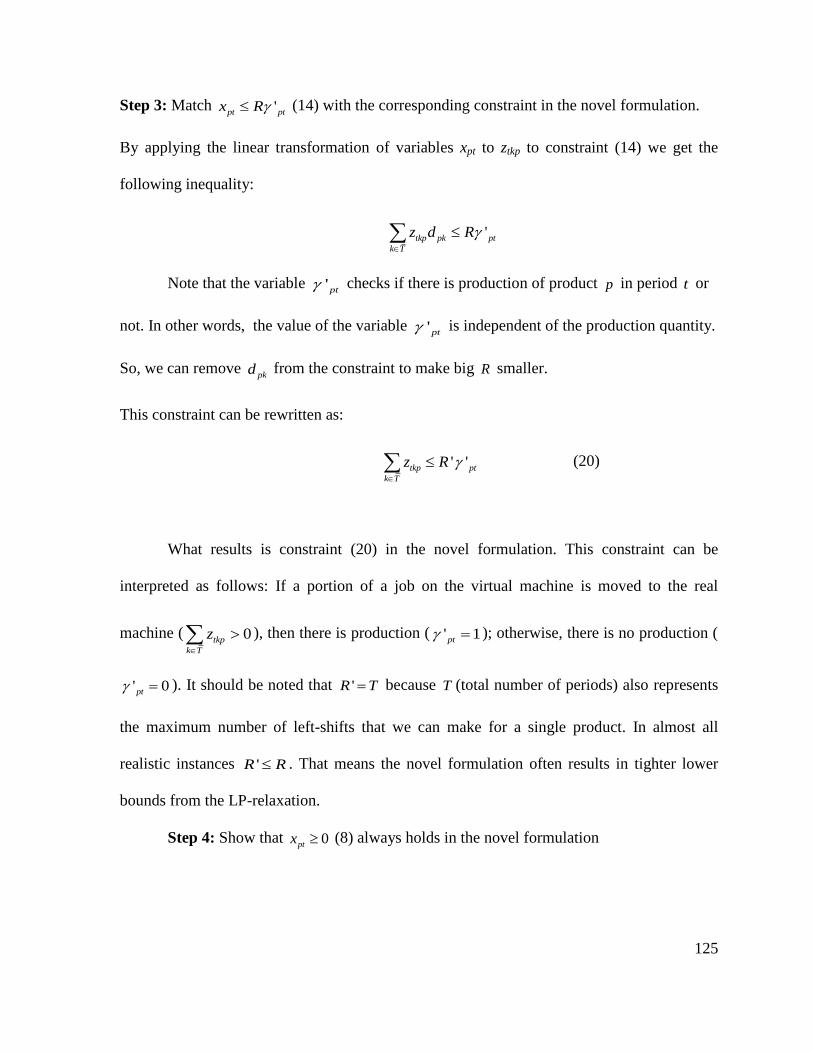
125

Step 3: Match 'pt ptx R (14) with the corresponding constraint in the novel formulation.

By applying the linear transformation of variables xpt to ztkp to constraint (14) we get the

following inequality:

'tkp pk pt

k T

z d R

Note that the variable 'pt checks if there is production of product p in period t or

not. In other words, the value of the variable 'pt is independent of the production quantity.

So, we can remove pkd from the constraint to make big R smaller.

This constraint can be rewritten as:

' 'tkp pt

k T

z R

(20)

What results is constraint (20) in the novel formulation. This constraint can be

interpreted as follows: If a portion of a job on the virtual machine is moved to the real

machine ( 0tkp

k T

z

), then there is production ( ' 1pt ); otherwise, there is no production (

' 0pt ). It should be noted that 'R T because T (total number of periods) also represents

the maximum number of left-shifts that we can make for a single product. In almost all

realistic instances 'R R . That means the novel formulation often results in tighter lower

bounds from the LP-relaxation.

Step 4: Show that 0ptx (8) always holds in the novel formulation

126

Replace ptx with

tkp pk

k T

z d

, such that

0tkp pk

k T

z d

.

The inequality above always holds because ptd

is always non-negative and

tpkz is always

non-negative by definition.

We have shown so far that constraints (4), (13) and (14) in the modified formulation

are equivalent to constraints (36), (19) and (20) in the novel formulation. In addition to that

we have proved that constraint (8) in the modified formulation always holds in the novel

formulation. If both formulations are compared, it can easily be seen that the remaining

constraints in the modified formulation are exactly the same as the corresponding constraints

in the novel formulation.

Step 5: The final step is to show that any feasible value of ptx can be represented in the

novel formulation in terms of the tkpz variables, and that any feasible solution of the novel

formulation is a feasible solution to the modified formulation. In other words, we need to

make sure that no extreme point is lost and no new point is generated during the redefinition

of the variables. Consider the same variable redefinition:

pt tkp pk

k T

x z d

.

We know that any optimal solution of the modified formulation has the following property:

0T

pt pa

a t

x d

.

127

That means we never produce more than the demand of the current period plus the

total demand of later periods. Since we do not allow backordering or lost sales, production in

later periods for previous periods is not allowed. To be able to claim that every optimal

solution of the modified formulation corresponds to an optimal solution in the novel

formulation we must show that the following inequality always holds in the novel

formulation:

0T

tkp pk pa

k T a t

z d d

We already showed that tkp pk

k T

z d

is always non-negative. Now we need to show that the

following inequality always holds in the novel formulation:

T

tkp pk pa

k T a t

z d d

(71)

We know that tkpz is only defined for k t . So the left hand-side of (71) can be written as:

, 1, , 1 , 2, , 2 , , ,...tkp pk t k p p k t k p p k t T p p Tz d z d z d z d

We also know that 0 1tkpz . To find the upper bound of the expression above replace z

variables with 1:

, 1 , 2 ,... T

pk p k p k p T pk

k t

d d d d d

.

If we plug this into (71) we get:

T T

pk pa

k t a t

d d

.

128

That means the maximum value of the left hand-side of inequality (71) is never greater than

the right hand-side. In other words, inequality (71) always holds in the novel formulation.

It is clear that tkp pk

k T

z d

can take any value between zero and T

pa

a t

d

by assigning

proper values to thetkpz variables. By that, we have shown that any optimal solution in one

formulation can be translated to an optimal solution in the other.

129

Appendix B

When the novel formulation was first written it was a little different than the version

that we have presented above. We call the first version of the novel formulation ―the novel

formulation before the improvement‖. Please note that the novel formulation before the

improvement allocates the jobs directly to the real-machine. The virtual machine

interpretation cannot be made. In this version of the novel formulation, z variables are not

defined for k t ; they are defined only for t k . In that case the following variable

redefinition should be used:

(1 )pt pt atp tap pa

a T a T

x d z z d

Alternative Novel Formulation

The alternative novel formulation starts with a ―lot-for-lot‖ plan and tries to improve

it by making ―left-shifts‖ so that the total setup cost is minimized. By ―lot for lot,‖ we mean

processing each job in its demand period without batching it with jobs from the same family

in other periods. ―Left-shift‖ is a common terminology in the literature, and it means moving

a job from a later period to an earlier one. The reason we shift a job to the left is to batch it

with another job from the same family and therefore to save a setup. Note that if production

of a product is scheduled after its demand period then the plan is infeasible. In other words,

in the lot-for-lot plan products are scheduled to be produced in the latest possible period. The

lot-for-lot plan might not be feasible due to capacity limitations, but if there is a feasible plan

then the novel formulation makes necessary left-shifts and finds it.

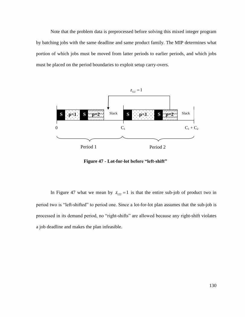
130

Note that the problem data is preprocessed before solving this mixed integer program

by batching jobs with the same deadline and same product family. The MIP determines what

portion of which jobs must be moved from latter periods to earlier periods, and which jobs

must be placed on the period boundaries to exploit setup carry-overs.

In Figure 47 what we mean by 122 1z is that the entire sub-job of product two in

period two is ―left-shifted‖ to period one. Since a lot-for-lot plan assumes that the sub-job is

processed in its demand period, no ―right-shifts‖ are allowed because any right-shift violates

a job deadline and makes the plan infeasible.

Figure 47 - Lot-for-lot before “left-shift”

S p=1 S p=2 S p=1 S p=2

Period 1 Period 2

C1

C1 + C2

0

Slack

Slack

1221z

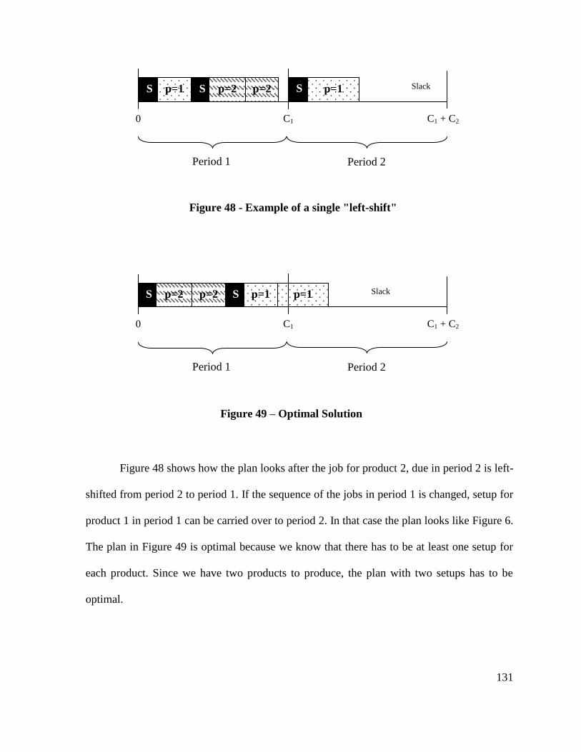
131

Figure 48 shows how the plan looks after the job for product 2, due in period 2 is left-

shifted from period 2 to period 1. If the sequence of the jobs in period 1 is changed, setup for

product 1 in period 1 can be carried over to period 2. In that case the plan looks like Figure 6.

The plan in Figure 49 is optimal because we know that there has to be at least one setup for

each product. Since we have two products to produce, the plan with two setups has to be

optimal.

S p=1 S p=2 p=1 p=2

Period 1 Period 2

C1

C1 + C2

0

Slack

S

Figure 48 - Example of a single "left-shift"

S p=1 S p=2 p=1 p=2

Period 1 Period 2

C1

C1 + C2

0

Slack

Figure 49 – Optimal Solution

132

Alternative Novel Formulation

Minimize 1( ' )s s

p pt p pt

p Pt T

c c

(72)

Subject to

, 1'u u u s s

tp p ktp tp p tkp pk p pt p p t p t

p P k T k T

d t z d t z d t t t C

t T (73)

' 'pt ktp tkp pt

k T k T

R z z y

,p P t T (74)

1pt

p P

t T

(75)

, 1 , 12 ' ' 0pt p t pt p t

,p P t T

(76)

1tkp

t T

z

,p P k T

(77)

tkp kpz y , ,p P t T k T

(78)

0 1tkpz , ,p P t T k T (79)

(80)

(81)

All the constraints and the objective function have the same interpretation as the novel

formulation.

0

0p p p P

{0,1} , ' {0,1}pt pt ,p P t T

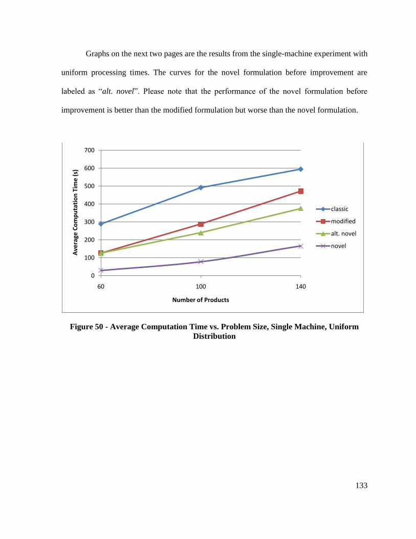
133

Graphs on the next two pages are the results from the single-machine experiment with

uniform processing times. The curves for the novel formulation before improvement are

labeled as ―alt. novel‖. Please note that the performance of the novel formulation before

improvement is better than the modified formulation but worse than the novel formulation.

Figure 50 - Average Computation Time vs. Problem Size, Single Machine, Uniform

Distribution

0

100

200

300

400

500

600

700

60 100 140

Ave

rage

Co

mp

uta

tio

n T

ime

(s)

Number of Products

classic

modified

alt. novel

novel

134

Figure 51 - Gap Performance, Single Machine, Uniform Distribution (Cumulative)


(Cumulative)

65%

70%

75%

80%

85%

90%

95%

100%

0.0% 0.5% 1.0% 1.5% 2.0% 2.5% 3.0% 3.5% 4.0% 4.5% 5.0%

% o

f in

stan

ces

solv

ed

Gap

classic

modified

alt. novel

novel

50%

55%

60%

65%

70%

75%

80%

85%

90%

95%

100%

0 100 200 300 400 500 600 700 800 900 1000 1100 1200

% o

f in

stan

ces

solv

ed

to

op

tim

alit

y

Time (s)

classic

modi

alt. novel

novel

135

Appendix C

In this Appendix, we present six graphs showing the relationship between the

percentage gap ∆ and the density and slackness parameters for the three formulations that we

analyzed in this study. The graphs demonstrate that if the classical and modified formulations

are used, the gap ∆ tends to be large in the high density and high slackness region. We do not

observe such behavior if the novel formulation is used.

Figure 53 - Gap vs. Density and Slackness, Classical Formulation, Two Machines,

Uniform Distribution, p=140

0

0.25

0.5

0.0%

2.0%

4.0%

6.0%

8.0%

0.5

0.7

0.9

Slac

kne

ss

∆ (

GA

P)

Density

136

Figure 54 - Gap vs. Density and Slackness, Modified Formulation, Two Machines,


Figure 55 - Gap vs. Density and Slackness, Novel Formulation, Two Machines, Uniform

Distribution, p=140

0

0.25

0.5

0.0%

2.0%

4.0%

6.0%

8.0%

0.5

0.7

0.9

Slac

kne

ss

∆ (

GA

P)

Density

0

0.25

0.5

0.0%

2.0%

4.0%

6.0%

8.0%

0.5

0.7

0.9

Slac

kne

ss

∆ (

GA

P)

Density

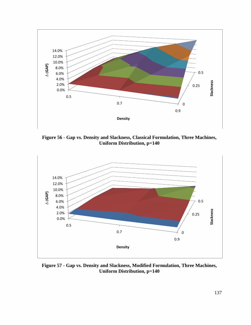
137

Figure 56 - Gap vs. Density and Slackness, Classical Formulation, Three Machines,


Figure 57 - Gap vs. Density and Slackness, Modified Formulation, Three Machines,


0

0.25

0.5

0.0%

2.0%

4.0%

6.0%

8.0%

10.0%

12.0%

14.0%

0.5

0.7

0.9

Slac

kne

ss

∆ (

GA

P)

Density

0

0.25

0.5

0.0%

2.0%

4.0%

6.0%

8.0%

10.0%

12.0%

14.0%

0.5

0.7

0.9

Slac

kne

ss

∆ (

GA

P)

Density

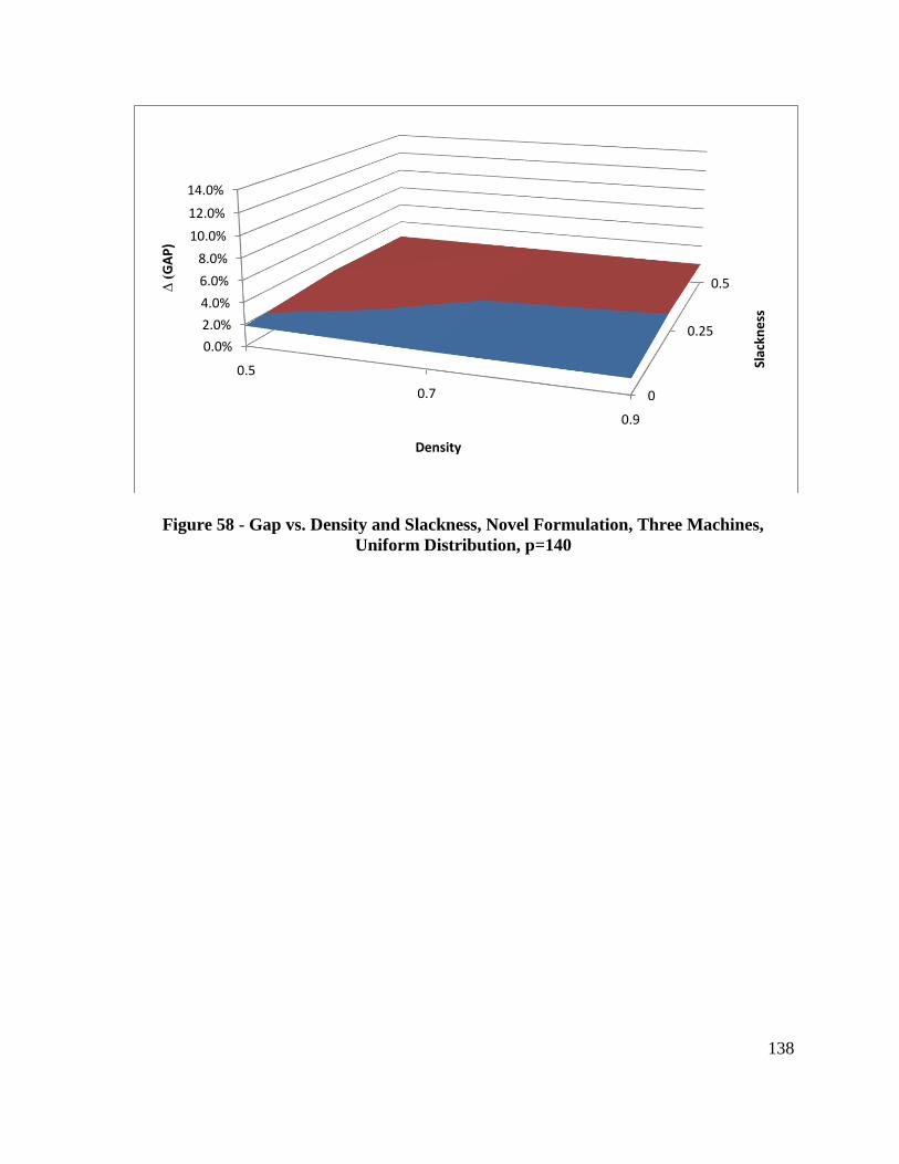
138

Figure 58 - Gap vs. Density and Slackness, Novel Formulation, Three Machines,


0

0.25

0.5

0.0%

2.0%

4.0%

6.0%

8.0%

10.0%

12.0%

14.0%

0.5

0.7

0.9

Slac

kne

ss

∆ (

GA

P)

Density

a novel solution approach to capacitated lot-sizing problems with setup times and setup carry-over

Documents

novel formulation

classical formulation

relaxed formulation

singlemachine formulation

bound solution process

bound solutions

bound trees

upper bound incumbent