A Fix-and-Optimize Approach for the Multi-Level

Capacitated Lot Sizing Problem

Stefan Helber, Florian Sahling

Leibniz Universitat Hannover

Institut fur Produktionswirtschaft

Konigsworther Platz 1

D-30167 Hannover

March 7, 2008

Abstract

This paper presents an optimization-based solution approach for the dy-

namic multi-level capacitated lot sizing problem (MLCLSP) with positive lead

times. The key idea is to solve a series of mixed-integer programs in an itera-

tive fix-and-optimize algorithm. Each of these programs is optimized over all

real-valued variables, but only a small subset of binary setup variables. The

remaining binary setup variables are tentatively fixed to values determined in

previous iterations. The resulting algorithm is transparent, flexible, accurate

and relatively fast. Its solution quality outperforms those of the approaches

by Tempelmeier/Derstroff and by Stadtler.

1 Introduction

This paper treats the problem to determine time-phased production quantities (lot

sizes) for multi-level production systems in which a changeover at a resource from

one product type to another requires a setup time and/or causes setup cost. The

capacity of the resources is limited. The time-phased demand is assumed to be

given and has to be satisfied. To date, this type of lot sizing problem cannot be

solved satisfactorily within computerized Material Requirements Planning (MRP)

modules of Enterprise Resource Planning (ERP) systems. The reason is that these

systems often ignore the capacity limits of the production system while computing

the lot sizes. This leads to infeasible production schedules which result in long and

unpredictable lead times and large in-process inventories.

1

The problem of finding capacity-feasible production quantities for a multi-stage

production system that minimize setup and holding cost has been formally stated as

the Multi-Level Capacitated Lot Sizing Problem (MLCLSP), see Billington (1983).

For capacitated production systems with non-zero setup times, the question whether

a feasible production plan (without overtime) exists has shown to be already NP-

complete, see Maes et al. (1991). Several authors have therefore developed heuristics

for the problem. Multi-level capacitated lot sizing is hence both practically impor-

tant and scientifically challenging.

From a practical point of view, generic lot sizing approaches for ERP systems

should meet several requirements. First, they should be adaptable to specific as-

pects of a concrete production system. This favors flexible approaches based on

mathematical programming as opposed to “hard-wired” procedural heuristics that

follow a highly problem-specific logic. Second, they should enable the planer to find

feasible solutions of acceptable quality quickly and then let him decide to invest

additional computation time to improve the solution. Third, if lot sizing on the

one hand and sequencing/scheduling on the other are treated separately, it should

always be possible to disaggregate the (aggregated) lot sizes into a detailed produc-

tion schedule in continuous time. In a multi-level production system, this can only

be guaranteed if positive lead times between the production stages are considered.

Reviews of the literature on dynamic lot sizing are given by Bahl et al. (1987),

Maes and van Wassenhove (1988), Gupta and Keung (1990), Salomon et al. (1991)

and Buschkuhl et al. (2008). Kuik et al. (1994) relate lot sizing to batching and

comment on some general criticism of batching analysis. The progress with single-

item lot sizing is analyzed by Wolsey (1995) and Brahimi et al. (2006). Drexl and

Kimms (1997) discuss models that consider both lot sizing and scheduling. Karimi

et al. (2003) give a review of solution approaches for single-stage capacitated lot siz-

ing problems and Jans and Degraeve (2007) focus on metaheuristics for dynamic lot

sizing. Table 1 classifies papers on the MLCLSP by the general solution approach,

i.e., mathematical programming-based approaches, Lagrangean relaxation and de-

composition, decomposition and aggregation, local search and metaheuristics and

finally greedy heuristics. Some of these papers are discussed below in more detail.

In Tempelmeier and Helber (1994), Helber (1995) and Tempelmeier and Derstroff

(1996), early product-oriented decomposition approaches for the MLCLSP are pre-

sented. The Tempelmeier/Destroff-heuristic (TDH) is until now the fastest available

method for the MLCLSP. It is based on a Lagrangean relaxation of the MLCLSP

which then decomposes into single-product uncapacitated lot sizing problems of the

type studied by Wagner and Whitin (1958). The Langrangean relaxation leads to a

lower bound on the objective function value. A heuristic finite scheduling procedure

is used to create a feasible solution and to compute an upper bound on the optimal

2

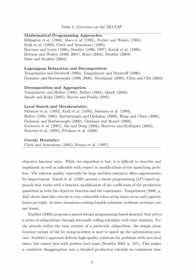
Table 1: Literature on the MLCLSP

Mathematical Programming ApproachesBillington et al. (1986), Maes et al. (1991), Pochet and Wolsey (1991),Kuik et al. (1993), Clark and Armentano (1995),Harrison and Lewis (1996), Stadtler (1996, 1997), Katok et al. (1998),Belvaux and Wolsey (2000, 2001), Rossi (2003), Stadtler (2003),Surie and Stadtler (2003)

Lagrangean Relaxation and DecompositionTempelmeier and Derstroff (1993), Tempelmeier and Derstroff (1996),

Ozdamar and Barbarosoglu (1999, 2000), Moorkanat (2000), Chen and Chu (2003)

Decomposition and AggregationTempelmeier and Helber (1994), Helber (1994), Quadt (2004),Quadt and Kuhn (2005), Boctor and Poulin (2005)

Local Search and MetaheuristicsSalomon et al. (1993), Kuik et al. (1993), Salomon et al. (1993),

Helber (1994, 1995), Barbarosoglu and Ozdamar (2000), Hung and Chien (2000),

Ozdamar and Barbarosoglu (2000), Ozdamar and Bozyel (2000),Gutierrez et al. (2001), Xie and Dong (2002), Berretta and Rodrigues (2004),Berretta et al. (2005), Pitakaso et al. (2006)

Greedy HeuristicsClark and Armentano (1995), Franca et al. (1997)

objective function value. While the algorithm is fast, it is difficult to describe and

implement as well as inflexible with respect to modifications of the underlying prob-

lem. The solution quality especially for large problem instances offers opportunities

for improvement. Katok et al. (1998) present a linear-programming (LP)-based ap-

proach that works with a heuristic modification of the coefficients of the production

quantities in both the objective function and the constraints. Tempelmeier (2006, p.

342) shows that this concept is very vulnerable when setup times occur and capacity

limits are tight. In these situations existing feasible solutions (without overtime) are

not found.

Stadtler (2003) proposes a mixed-integer programming-based heuristic that solves

a series of subproblems through internally rolling schedules with time windows. For

the periods within the time window of a particular subproblem, the simple plant

location variant of the lot sizing problem is used to speed up the optimization pro-

cess. Stadtler’s approach delivers high-quality solutions for problems with zero lead

times, but cannot deal with positive lead times (Stadtler 2003, p. 501). This makes

a consistent disaggregation into a detailed production schedule in continuous time

3

impossible. In addition, solution times for his approach increase substantially as the

problem size (number of binary setup variables) increases. A variant of Stadtler’s

general approach of internally rolling schedules for the Capacitated Lot Sizing Prob-

lem with Linked Lot Sizes (Haase 1994, 1998) is presented by Surie and Stadtler

(2003). It is based on an extended model formulation and valid inequalities to yield

a tight formulation that speeds up the branch&bound process. Belvaux and Wolsey

(2001) show how to develop tight formulations for several special problem features

occurring in practice. Rossi (2003) develops a time-oriented decomposition similar

to the one by Stadtler where some of the setup variables are initially relaxed while

others are iteratively fixed. Unfortunately, the author provides no direct compar-

ison to the procedures by Stadtler and by Tempelmeier and Derstroff. Pitakaso

et al. (2006) present a decomposition algorithm for the MLCLSP based on a lim-

ited subset of products and periods. Each problem in the decomposition is solved

to optimality and a capacity reservation mechanism is used to reflect products and

periods “outside” of the current problem. The decomposition itself is controlled by

an “ant colony optimization” algorithm. The computation times that are necessary

to find better results than with Stadtler’s method appear to be quite high (20 to

30 minutes) and then the average improvement is small. Berretta and Rodrigues

(2004) describe a memetic algorithm which is also population-based. However, they

compare their results to those presented by Tempelmeier and Derstroff only for tiny

problems with 40 binary variables. The picture is similar for a similar algorithm

by Berretta et al. (2005): Relatively large deviations from optimal solutions occur

already for problems with only 60 binary variables.

In this paper we present a mathematical programming-based algorithm for the

MLCLSP that is flexible and transparent, that allows to trade in solution time for

solution quality and that can deal with positive lead times. In an iterative fix-

and-optimize approach (Pochet and Wolsey 2006, p. 113, call this “Exchange”), a

sequence of mixed-integer programs (MIPs) is solved over all real-valued decision

variables and a subset of the binary setup variables. The solution with respect to

the binary variables is a fixed parameter for the next MIPs that optimize other

binary variables. The optimization of the algebraic decision model is done within

the MIP solver and therefore the approach is flexible. The user can trade in solution

time for solution quality by deciding about the number of binary variables to be

treated within a single MIP and about the number of iterations in which these are

optimized and fixed again. Even large problem instances from the literature can

be solved with a high solution quality within seconds or few minutes. We study

both the cases of zero and of positive lead times and compare our results to those

for the approaches by Tempelmeier and Derstroff (1996) and Stadtler (2003) in an

extensive numerical study. While the method by Tempelmeier and Derstroff (1996)

4

Table 2: Notation for the MLCLSPSets:k, i ∈ K productst ∈ T periodsj ∈ J resourcesKj set of products requiring resource jNk set of immediate successors of product k

Parameters:aki number of units of product k required to produce one unit of product ibjt available capacity of resource j in period tB big numberdkt external demand of product k in period thk holding cost of product k per unit and periodocjt overtime cost per unit of overtime at resource j in period tsk setup cost of product ktpk production time per unit of product ktsk setup time of product kzk planned lead time of product k

Decision variables:Ojt overtime at resource j in period tQkt production quantity (lot size) of product k in period tYkt planned end-of-period inventory of product k in period tγkt binary setup variable of product k in period t

is extremely fast (and much faster than ours), our method yields a substantially

higher solution quality. It outperforms the one presented by Stadtler (2003) with

respect to both solution quality and computation time.

The remainder of this paper is organized as follows: In Section 2 we give a formal

definition of the MLCLSP. The algorithm to solve the problem is presented in Sec-

tion 3. Numerical results comparing our method to those developed by Tempelmeier

and Derstroff and by Stadtler are reported in Section 4. The paper ends with some

conclusions and suggestions for further research (Section 5).

2 Problem Statement and Model Formulation

The objective of the MLCLSP is to determine production quantities Qkt and

end-of-period inventory levels Ykt of product k in period t so that the sum of setup,

holding and overtime cost is minimized. The demand dkt per product and period

at each production stage is given and has to be satisfied. Whenever a product is

produced during a period, a setup is required during this period which results in

5

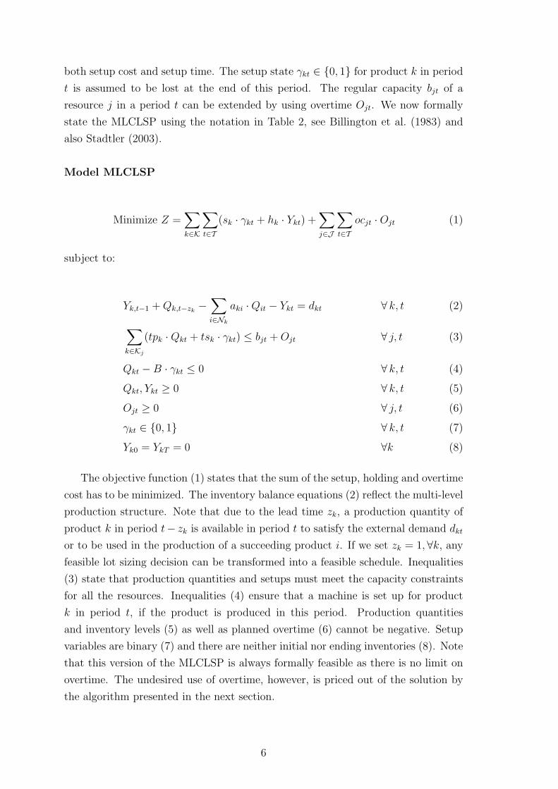
both setup cost and setup time. The setup state γkt ∈ {0, 1} for product k in period

t is assumed to be lost at the end of this period. The regular capacity bjt of a

resource j in a period t can be extended by using overtime Ojt. We now formally

state the MLCLSP using the notation in Table 2, see Billington et al. (1983) and

also Stadtler (2003).

Model MLCLSP

Minimize Z =∑k∈K

∑t∈T

(sk · γkt + hk · Ykt) +∑j∈J

∑t∈T

ocjt ·Ojt (1)

subject to:

Yk,t−1 + Qk,t−zk−

∑i∈Nk

aki ·Qit − Ykt = dkt ∀ k, t (2)∑k∈Kj

(tpk ·Qkt + tsk · γkt) ≤ bjt + Ojt ∀ j, t (3)

Qkt −B · γkt ≤ 0 ∀ k, t (4)

Qkt, Ykt ≥ 0 ∀ k, t (5)

Ojt ≥ 0 ∀ j, t (6)

γkt ∈ {0, 1} ∀ k, t (7)

Yk0 = YkT = 0 ∀k (8)

The objective function (1) states that the sum of the setup, holding and overtime

cost has to be minimized. The inventory balance equations (2) reflect the multi-level

production structure. Note that due to the lead time zk, a production quantity of

product k in period t− zk is available in period t to satisfy the external demand dkt

or to be used in the production of a succeeding product i. If we set zk = 1,∀k, any

feasible lot sizing decision can be transformed into a feasible schedule. Inequalities

(3) state that production quantities and setups must meet the capacity constraints

for all the resources. Inequalities (4) ensure that a machine is set up for product

k in period t, if the product is produced in this period. Production quantities

and inventory levels (5) as well as planned overtime (6) cannot be negative. Setup

variables are binary (7) and there are neither initial nor ending inventories (8). Note

that this version of the MLCLSP is always formally feasible as there is no limit on

overtime. The undesired use of overtime, however, is priced out of the solution by

the algorithm presented in the next section.

6

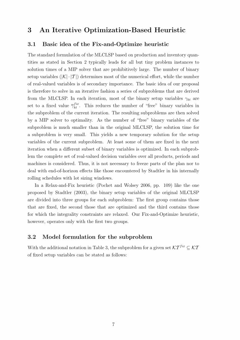
3 An Iterative Optimization-Based Heuristic

3.1 Basic idea of the Fix-and-Optimize heuristic

The standard formulation of the MLCLSP based on production and inventory quan-

tities as stated in Section 2 typically leads for all but tiny problem instances to

solution times of a MIP solver that are prohibitively large. The number of binary

setup variables (|K| · |T |) determines most of the numerical effort, while the number

of real-valued variables is of secondary importance. The basic idea of our proposal

is therefore to solve in an iterative fashion a series of subproblems that are derived

from the MLCLSP. In each iteration, most of the binary setup variables γkt are

set to a fixed value γfixkt . This reduces the number of “free” binary variables in

the subproblem of the current iteration. The resulting subproblems are then solved

by a MIP solver to optimality. As the number of “free” binary variables of the

subproblem is much smaller than in the original MLCLSP, the solution time for

a subproblem is very small. This yields a new temporary solution for the setup

variables of the current subproblem. At least some of them are fixed in the next

iteration when a different subset of binary variables is optimized. In each subprob-

lem the complete set of real-valued decision variables over all products, periods and

machines is considered. Thus, it is not necessary to freeze parts of the plan nor to

deal with end-of-horizon effects like those encountered by Stadtler in his internally

rolling schedules with lot sizing windows.

In a Relax-and-Fix heuristic (Pochet and Wolsey 2006, pp. 109) like the one

proposed by Stadtler (2003), the binary setup variables of the original MLCLSP

are divided into three groups for each subproblem: The first group contains those

that are fixed, the second those that are optimized and the third contains those

for which the integrality constraints are relaxed. Our Fix-and-Optimize heuristic,

however, operates only with the first two groups.

3.2 Model formulation for the subproblem

With the additional notation in Table 3, the subproblem for a given set KT fix ⊆ KTof fixed setup variables can be stated as follows:

7

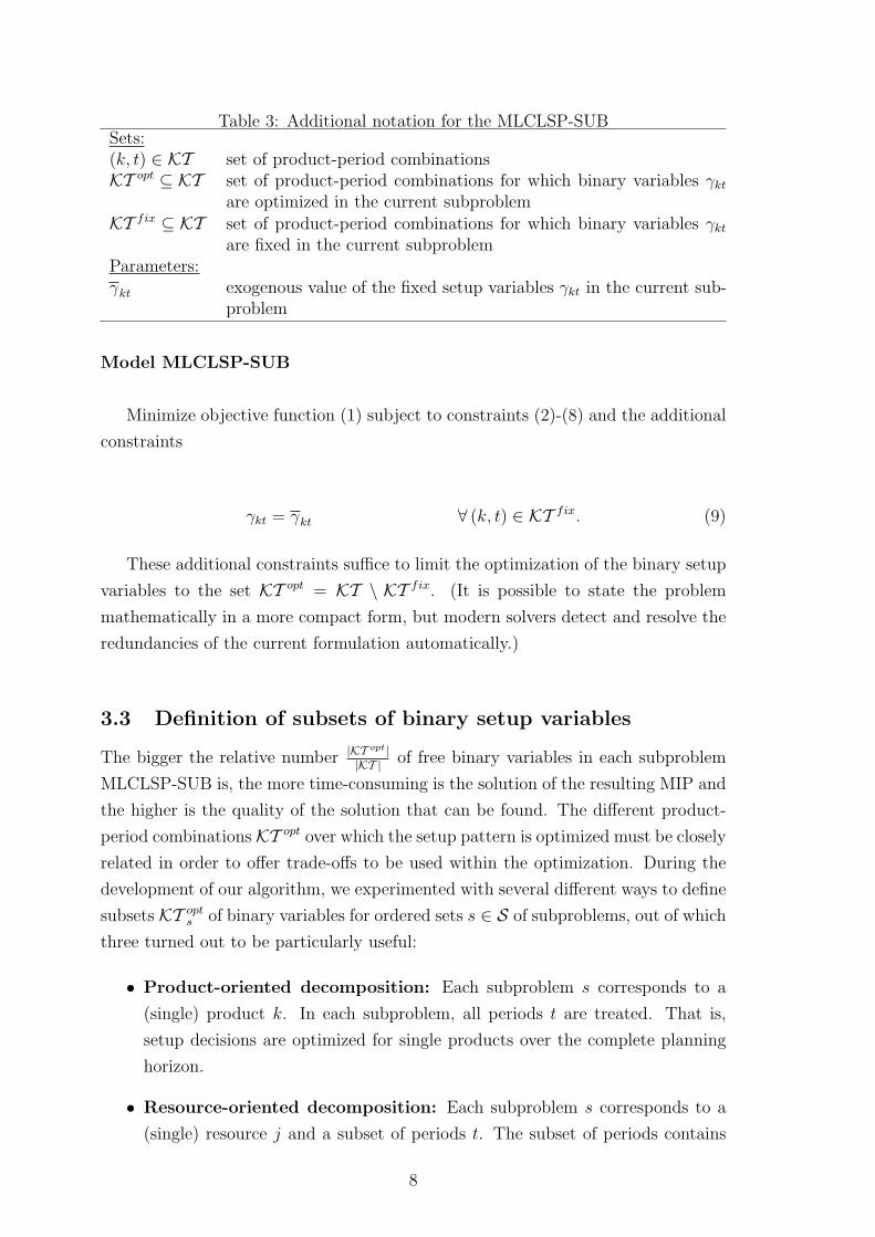
Table 3: Additional notation for the MLCLSP-SUBSets:(k, t) ∈ KT set of product-period combinationsKT opt ⊆ KT set of product-period combinations for which binary variables γkt

are optimized in the current subproblemKT fix ⊆ KT set of product-period combinations for which binary variables γkt

are fixed in the current subproblemParameters:γkt exogenous value of the fixed setup variables γkt in the current sub-

problem

Model MLCLSP-SUB

Minimize objective function (1) subject to constraints (2)-(8) and the additional

constraints

γkt = γkt ∀ (k, t) ∈ KT fix. (9)

These additional constraints suffice to limit the optimization of the binary setup

variables to the set KT opt = KT \ KT fix. (It is possible to state the problem

mathematically in a more compact form, but modern solvers detect and resolve the

redundancies of the current formulation automatically.)

3.3 Definition of subsets of binary setup variables

The bigger the relative number |KT opt||KT | of free binary variables in each subproblem

MLCLSP-SUB is, the more time-consuming is the solution of the resulting MIP and

the higher is the quality of the solution that can be found. The different product-

period combinations KT opt over which the setup pattern is optimized must be closely

related in order to offer trade-offs to be used within the optimization. During the

development of our algorithm, we experimented with several different ways to define

subsets KT opts of binary variables for ordered sets s ∈ S of subproblems, out of which

three turned out to be particularly useful:

• Product-oriented decomposition: Each subproblem s corresponds to a

(single) product k. In each subproblem, all periods t are treated. That is,

setup decisions are optimized for single products over the complete planning

horizon.

• Resource-oriented decomposition: Each subproblem s corresponds to a

(single) resource j and a subset of periods t. The subset of periods contains

8

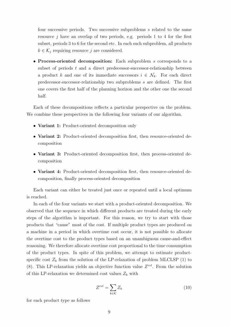
four successive periods. Two successive subproblems s related to the same

resource j have an overlap of two periods, e.g. periods 1 to 4 for the first

subset, periods 3 to 6 for the second etc. In each such subproblem, all products

k ∈ Kj requiring resource j are considered.

• Process-oriented decomposition: Each subproblem s corresponds to a

subset of periods t and a direct predecessor-successor-relationship between

a product k and one of its immediate successors i ∈ Nk. For each direct

predecessor-successor-relationship two subproblems s are defined. The first

one covers the first half of the planning horizon and the other one the second

half.

Each of these decompositions reflects a particular perspective on the problem.

We combine these perspectives in the following four variants of our algorithm.

• Variant 1: Product-oriented decomposition only

• Variant 2: Product-oriented decomposition first, then resource-oriented de-

composition

• Variant 3: Product-oriented decomposition first, then process-oriented de-

composition

• Variant 4: Product-oriented decomposition first, then resource-oriented de-

composition, finally process-oriented decomposition

Each variant can either be treated just once or repeated until a local optimum

is reached.

In each of the four variants we start with a product-oriented decomposition. We

observed that the sequence in which different products are treated during the early

steps of the algorithm is important. For this reason, we try to start with those

products that “cause” most of the cost. If multiple product types are produced on

a machine in a period in which overtime cost occur, it is not possible to allocate

the overtime cost to the product types based on an unambiguous cause-and-effect

reasoning. We therefore allocate overtime cost proportional to the time consumption

of the product types. In spite of this problem, we attempt to estimate product-

specific cost Zk from the solution of the LP-relaxation of problem MLCLSP (1) to

(8). This LP-relaxation yields an objective function value Zrel. From the solution

of this LP-relaxation we determined cost values Zk with

Zrel =∑k∈K

Zk (10)

for each product type as follows

9

Zk =∑t∈T

(sk · γrelkt + hk · Ykt) +

∑t∈T (tpk ·Qkt + tsk · γrel

kt )(∑

t∈T ocj(k),tOj(k),t

)∑k∈Kj(k)

∑t∈T (tpk ·Qkt + tsk · γrel

kt)

(11)

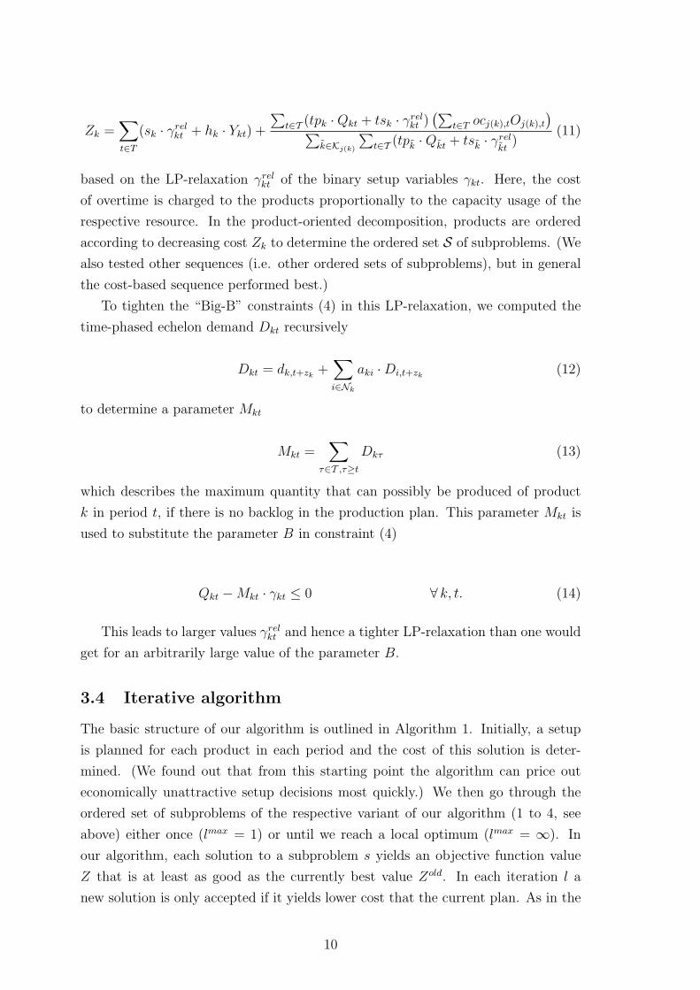
based on the LP-relaxation γrelkt of the binary setup variables γkt. Here, the cost

of overtime is charged to the products proportionally to the capacity usage of the

respective resource. In the product-oriented decomposition, products are ordered

according to decreasing cost Zk to determine the ordered set S of subproblems. (We

also tested other sequences (i.e. other ordered sets of subproblems), but in general

the cost-based sequence performed best.)

To tighten the “Big-B” constraints (4) in this LP-relaxation, we computed the

time-phased echelon demand Dkt recursively

Dkt = dk,t+zk+

∑i∈Nk

aki ·Di,t+zk(12)

to determine a parameter Mkt

Mkt =∑

τ∈T ,τ≥t

Dkτ (13)

which describes the maximum quantity that can possibly be produced of product

k in period t, if there is no backlog in the production plan. This parameter Mkt is

used to substitute the parameter B in constraint (4)

Qkt −Mkt · γkt ≤ 0 ∀ k, t. (14)

This leads to larger values γrelkt and hence a tighter LP-relaxation than one would

get for an arbitrarily large value of the parameter B.

3.4 Iterative algorithm

The basic structure of our algorithm is outlined in Algorithm 1. Initially, a setup

is planned for each product in each period and the cost of this solution is deter-

mined. (We found out that from this starting point the algorithm can price out

economically unattractive setup decisions most quickly.) We then go through the

ordered set of subproblems of the respective variant of our algorithm (1 to 4, see

above) either once (lmax = 1) or until we reach a local optimum (lmax = ∞). In

our algorithm, each solution to a subproblem s yields an objective function value

Z that is at least as good as the currently best value Zold. In each iteration l a

new solution is only accepted if it yields lower cost that the current plan. As in the

10

approach proposed by Stadtler (2003, p. 495) a capacity infeasible solution (with

overtime) is never considered as a candidate for a best solution, if there is already a

known capacity feasible solution. The boolean variable CapFeas indicates whether

a capacity feasible solution has already been found.

Algorithm 1 Two-phase algorithm

γkt = 1,∀(k, t) ∈ KTKT fix ← KTsolve MLCLSP-SUB and determine objective function value ZZnew = Zif

∑j∈J

∑t∈T Ojt = 0 then

CapFeas= yeselse

CapFeas= noend ifl=0repeat

l=l+1Zold = Znew

for each decomposition S in the current variant of the algorithm dofor each subproblem s ∈ S do

determine KT opts and KT fix

s = KT \KT opts for subproblem s

solve MLCLSP-SUB and determine objective function value Zif

∑j∈J

∑t∈T Ojt = 0 then

CapFeasnew= yeselse

CapFeasnew= noend ifif Z < Zold and (CapFeasnew or (not(CapFeasnew) and not(CapFeas))then

γkt = γkt,∀(k, t) ∈ KT opts

Znew = Zif CapFeasnew then

CapFeas= yesend if

end ifend for

end foruntil l = lmax or Znew ≥= Zold

Our algorithm was implemented in Delphi and we used the CPLEX 10.2 callable

library to solve the MIPs on a 2.13 GHz Intel Pentium Core2 machine with 4 GB

of RAM.

11

4 Numerical Results

4.1 Test sets and reference values

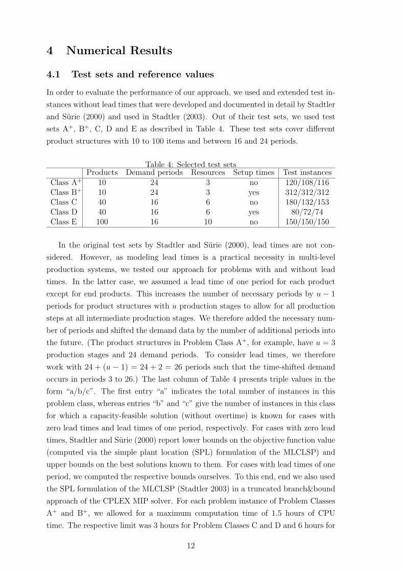
In order to evaluate the performance of our approach, we used and extended test in-

stances without lead times that were developed and documented in detail by Stadtler

and Surie (2000) and used in Stadtler (2003). Out of their test sets, we used test

sets A+, B+, C, D and E as described in Table 4. These test sets cover different

product structures with 10 to 100 items and between 16 and 24 periods.

Table 4: Selected test setsProducts Demand periods Resources Setup times Test instances

Class A+ 10 24 3 no 120/108/116Class B+ 10 24 3 yes 312/312/312Class C 40 16 6 no 180/132/153Class D 40 16 6 yes 80/72/74Class E 100 16 10 no 150/150/150

In the original test sets by Stadtler and Surie (2000), lead times are not con-

sidered. However, as modeling lead times is a practical necessity in multi-level

production systems, we tested our approach for problems with and without lead

times. In the latter case, we assumed a lead time of one period for each product

except for end products. This increases the number of necessary periods by u − 1

periods for product structures with u production stages to allow for all production

steps at all intermediate production stages. We therefore added the necessary num-

ber of periods and shifted the demand data by the number of additional periods into

the future. (The product structures in Problem Class A+, for example, have u = 3

production stages and 24 demand periods. To consider lead times, we therefore

work with 24 + (u − 1) = 24 + 2 = 26 periods such that the time-shifted demand

occurs in periods 3 to 26.) The last column of Table 4 presents triple values in the

form “a/b/c”. The first entry “a” indicates the total number of instances in this

problem class, whereas entries “b” and “c” give the number of instances in this class

for which a capacity-feasible solution (without overtime) is known for cases with

zero lead times and lead times of one period, respectively. For cases with zero lead

times, Stadtler and Surie (2000) report lower bounds on the objective function value

(computed via the simple plant location (SPL) formulation of the MLCLSP) and

upper bounds on the best solutions known to them. For cases with lead times of one

period, we computed the respective bounds ourselves. To this end, end we also used

the SPL formulation of the MLCLSP (Stadtler 2003) in a truncated branch&bound

approach of the CPLEX MIP solver. For each problem instance of Problem Classes

A+ and B+, we allowed for a maximum computation time of 1.5 hours of CPU

time. The respective limit was 3 hours for Problem Classes C and D and 6 hours for

12

Problem Class E. In our numerical study, we only tested the different algorithms on

those subsets of the test instances for which solutions without overtime are known.

We compare our results to those obtained by the Lagrangean decomposition

method developed by Tempelmeier and Derstroff (1996) and the time decomposition

approach by Stadtler (2003). Both authors provided us with an implementation of

their respective method to allow for a fair comparison. For problem instances with-

out lead times, we were able to compare our results to both competing approaches.

For the instances with lead times, our approach can only be compared to the one by

Tempelmeier and Derstroff (1996) as Stadtler’s time decomposition cannot deal with

lead times. It should also be noted that the implementation of the Tempelmeier-

Derstroff-Heuristic (TDH) (courtesy of Tempelmeier’s group) occasionally led to

solutions with some (very small) overtime use. For this reason, we decided to take

the setup pattern from the TDH solution and to re-compute the production plan by

solving the remaining linear program with real-valued decision variables, given this

setup pattern. We found that this additional step led to production quantities that

were indeed capacity feasible (without overtime) and report the objective function

values for these slightly better solutions of a “polished version” of the TDH.

We found that the method proposed by Stadtler is quite time-consuming. The

implementation of the algorithm (courtesy of Stadtler’s group) in XPRESSMP (rel.

17) has an option to impose a limit on the computation time. However, this limit

takes effect only if a first feasible solution has been found. For each problem class

we determined the maximum computation time of each combination of problem

instance and algorithmic variant of our method. We imposed this maximum value

as a time limit for Stadtler’s method. In several cases Stadtler’s method required

more than this time limit to find a first feasible solution. Stadtler’s method operates

with moving time windows. Based on the parameter settings that he reported to be

quite powerful, we used his algorithm with a time window of four successive periods

(none of them with a relaxed integrality constraint). In the next iteration, we moved

this time window one period into the future. In Stadtler’s terms, we worked with a

“4/0/1” parameter setting.

Depending on the variant of our algorithm as described in Section 3, in each

instance of Problem Classes A+ and B+, we optimized over 3% to 10% of the bi-

nary setup variables, i.e. 0.03 ≤ |KT opt

KT | ≤ 0.1 in any one instance of Problem

MLCLSP-SUB. For the larger problem instances with more products, this fraction

of optimized binary variables was smaller. When dealing with Problem Classes C

and D, only 1% to 7.5% of the binary variables were optimized in a single instance

of Problem MLCLSP-SUB. For Problem Class E, this range was 0.5% to 4% of the

setup variables.

13

4.2 Results for problem instances without lead times

The results for problem instances without lead times are presented in Tables 5

to 7. We report for the approach by Tempelmeier and Derstroff (TDH), by Stadtler

(StaH) and the four variants of our algorithm the following values: “ADUB” denotes

the average relative deviation of the solution from the best known upper bound as

reported by Stadtler and Surie. “ADLB” denotes the average relative deviation of

the respective heuristic solution from the lower bound as reported by Stadtler and

Surie. “Feas” is the fraction of problem instances that could be solved without the

use of overtime (which is extremely costly in all the instances) and “Time” is the

computation time.

The results show the following: The heuristic by Tempelmeier and Derstroff

is so fast (compared to all other approaches) that its computation time can in

fact be neglected. For problems without lead times, however, it yields the worst

solution quality if compared to the approach by Stadtler and to most variants of

our method. If one allows for multiple iterations of Variants 2 to 4 of our method,

it outperforms Stadtler’s method both with respect to the computation time and to

the quality of the solution, even though the improvement of the solution quality is

limited. It is also interesting to note that on average a single iteration of Variant 4

of our algorithm yields better solutions than multiple iterations of Variant 1 of the

method. This indicates that changing the perspective in the process of optimizing

the setup pattern is a worthwhile undertaking. The results also indicate that it is in

general useful to go through multiple iterations of any variant of the algorithm until

a local optimum is found. The percentage increase of the solution time appears

to be no more than about 50% of the time for a single iteration. Note that for

Problem Classes C and E, the average time required for Stadtler’s method to find a

capacity feasible solution (without overtime) extended the time limit derived from

the maximum solution time of our method as explained in Section 4.1.

4.3 Results for problem instances with lead times

In Tables 8, 9 and the right hand part of Table 7 we present the results for lead

times of one period. (Remember that for these instances Stadtler’s method cannot

be applied.) The results look very similar to those for problem instances without

lead times. If one has to deal with lead times, our method is the one that currently

delivers the highest solution quality.

14

Table 5: Results for Class A+ and Class B+ without leadtimes

Problem Class A+ Problem Class B+

ADUB ADLB Feas Time ADUB ADLB Feas Time[%] [%] [%] [sec] [%] [%] [%] [sec]

TDH 13.19 37.95 100.00 0.08 12.52 37.28 100.00 0.08Sta 4.14 26.31 99.07 13.49a 4.11 24.18 84.62 13.50b

Single iteration (lmax = 1)

Var 1 4.09 26.50 100.00 1.16 3.82 26.42 100.00 1.56Var 2 1.80 23.79 100.00 2.72 1.52 23.55 100.00 3.32Var 3 2.13 24.20 100.00 3.03 1.96 24.13 100.00 3.39Var 4 1.31 23.21 100.00 4.27 0.99 22.91 100.00 6.18

Multiple iterations (lmax =∞)

Var 1 2.51 24.66 100.00 1.71 2.20 24.40 100.00 2.08Var 2 1.03 22.87 100.00 4.42 0.62 22.43 100.00 5.24Var 3 1.67 23.65 100.00 3.75 1.30 23.31 100.00 5.13Var 4 0.78 22.58 100.00 6.38 0.41 22.20 100.00 8.40

aMaximum allowed solution time: 14 secbMaximum allowed solution time: 22 sec

Table 6: Results for Class C and Class D without leadtimes

Problem Class C Problem Class D

ADUB ADLB Feas Time ADUB ADLB Feas Time[%] [%] [%] [sec] [%] [%] [%] [sec]

TDH 6.76 23.07 100.00 0.43 5.68 14.80 100.00 0.28Sta 2.14 18.33 99.24 279.21a 6.99 14.96 88.89 76.73b

Single iteration (lmax = 1)

Var 1 8.32 25.66 100.00 3.83 10.34 19.78 100.00 3.59Var 2 3.80 20.44 100.00 13.80 4.96 13.89 100.00 7.48Var 3 4.81 21.65 100.00 16.72 5.33 14.33 100.00 11.45Var 4 2.71 19.21 100.00 28.82 3.82 12.66 100.00 17.23

Multiple iterations (lmax =∞)

Var 1 5.14 22.03 100.00 7.29 5.28 14.27 100.00 6.20Var 2 1.57 17.85 100.00 26.40 2.72 11.45 100.00 10.96Var 3 3.71 20.40 100.00 33.88 4.36 13.26 100.00 19.72Var 4 1.16 17.40 100.00 40.90 2.17 10.87 100.00 34.40

aMaximum allowed solution time: 263 secbMaximum allowed solution time: 81 sec

5 Conclusions and Outlook

We have presented an mathematical-programming-based approach to solve the ML-

CLSP with lead times. Modeling lead times is necessary, if one wants to be able

15

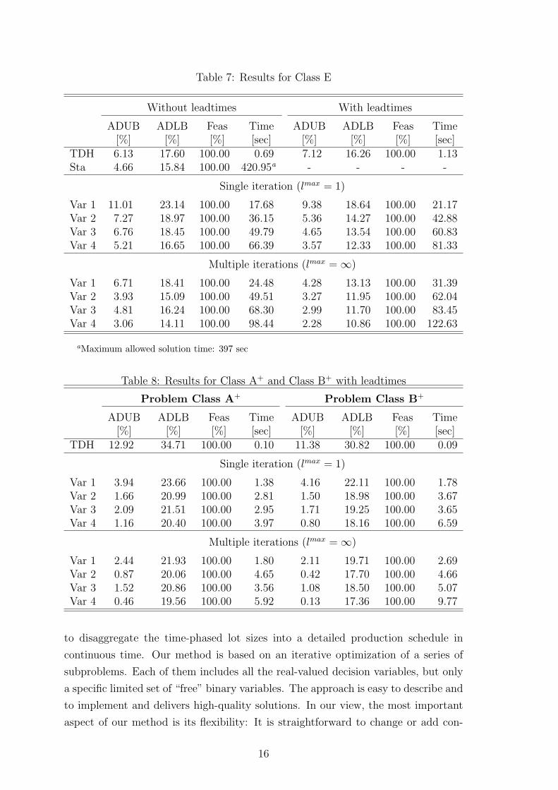
Table 7: Results for Class E

Without leadtimes With leadtimes

ADUB ADLB Feas Time ADUB ADLB Feas Time[%] [%] [%] [sec] [%] [%] [%] [sec]

TDH 6.13 17.60 100.00 0.69 7.12 16.26 100.00 1.13Sta 4.66 15.84 100.00 420.95a - - - -

Single iteration (lmax = 1)

Var 1 11.01 23.14 100.00 17.68 9.38 18.64 100.00 21.17Var 2 7.27 18.97 100.00 36.15 5.36 14.27 100.00 42.88Var 3 6.76 18.45 100.00 49.79 4.65 13.54 100.00 60.83Var 4 5.21 16.65 100.00 66.39 3.57 12.33 100.00 81.33

Multiple iterations (lmax =∞)

Var 1 6.71 18.41 100.00 24.48 4.28 13.13 100.00 31.39Var 2 3.93 15.09 100.00 49.51 3.27 11.95 100.00 62.04Var 3 4.81 16.24 100.00 68.30 2.99 11.70 100.00 83.45Var 4 3.06 14.11 100.00 98.44 2.28 10.86 100.00 122.63

aMaximum allowed solution time: 397 sec

Table 8: Results for Class A+ and Class B+ with leadtimes

Problem Class A+ Problem Class B+

ADUB ADLB Feas Time ADUB ADLB Feas Time[%] [%] [%] [sec] [%] [%] [%] [sec]

TDH 12.92 34.71 100.00 0.10 11.38 30.82 100.00 0.09

Single iteration (lmax = 1)

Var 1 3.94 23.66 100.00 1.38 4.16 22.11 100.00 1.78Var 2 1.66 20.99 100.00 2.81 1.50 18.98 100.00 3.67Var 3 2.09 21.51 100.00 2.95 1.71 19.25 100.00 3.65Var 4 1.16 20.40 100.00 3.97 0.80 18.16 100.00 6.59

Multiple iterations (lmax =∞)

Var 1 2.44 21.93 100.00 1.80 2.11 19.71 100.00 2.69Var 2 0.87 20.06 100.00 4.65 0.42 17.70 100.00 4.66Var 3 1.52 20.86 100.00 3.56 1.08 18.50 100.00 5.07Var 4 0.46 19.56 100.00 5.92 0.13 17.36 100.00 9.77

to disaggregate the time-phased lot sizes into a detailed production schedule in

continuous time. Our method is based on an iterative optimization of a series of

subproblems. Each of them includes all the real-valued decision variables, but only

a specific limited set of “free” binary variables. The approach is easy to describe and

to implement and delivers high-quality solutions. In our view, the most important

aspect of our method is its flexibility: It is straightforward to change or add con-

16

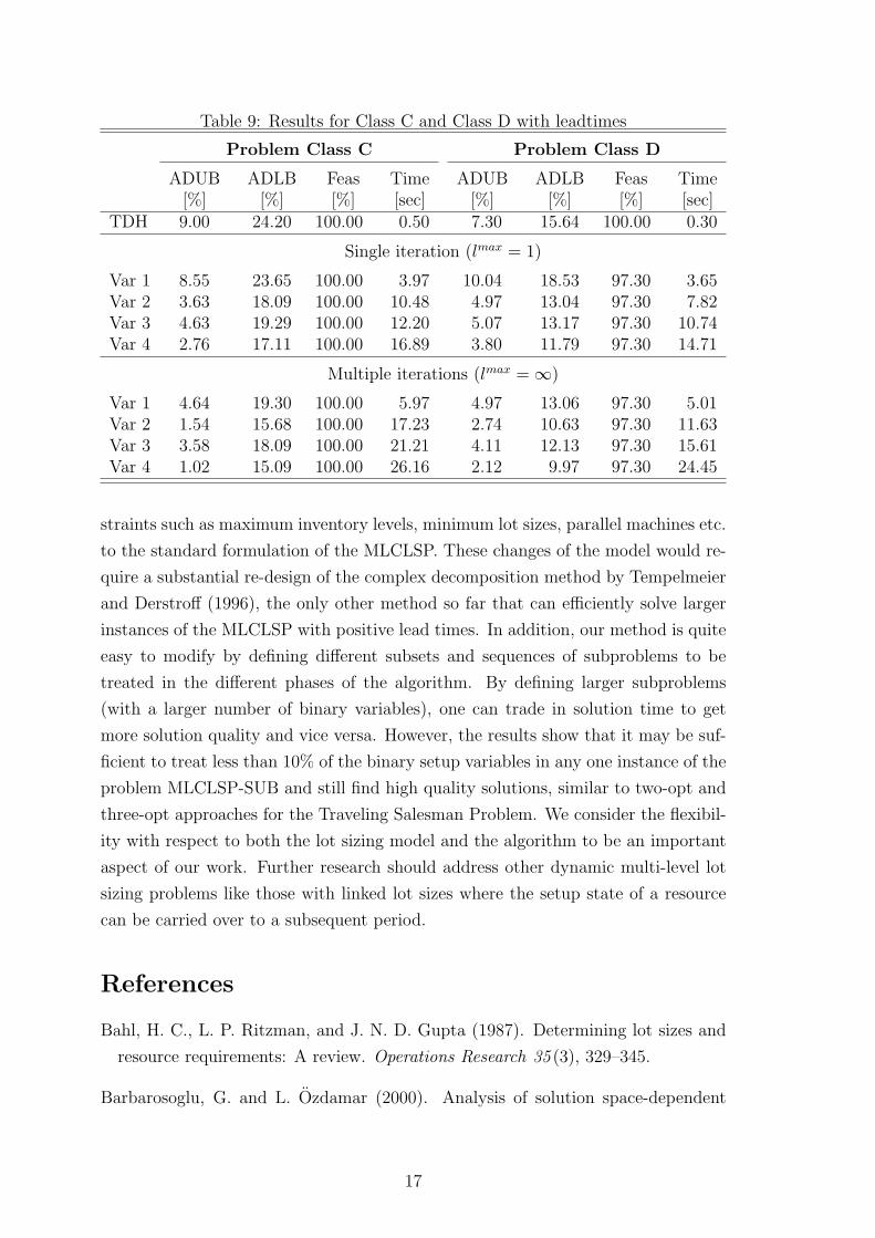
Table 9: Results for Class C and Class D with leadtimes

Problem Class C Problem Class D

ADUB ADLB Feas Time ADUB ADLB Feas Time[%] [%] [%] [sec] [%] [%] [%] [sec]

TDH 9.00 24.20 100.00 0.50 7.30 15.64 100.00 0.30

Single iteration (lmax = 1)

Var 1 8.55 23.65 100.00 3.97 10.04 18.53 97.30 3.65Var 2 3.63 18.09 100.00 10.48 4.97 13.04 97.30 7.82Var 3 4.63 19.29 100.00 12.20 5.07 13.17 97.30 10.74Var 4 2.76 17.11 100.00 16.89 3.80 11.79 97.30 14.71

Multiple iterations (lmax =∞)

Var 1 4.64 19.30 100.00 5.97 4.97 13.06 97.30 5.01Var 2 1.54 15.68 100.00 17.23 2.74 10.63 97.30 11.63Var 3 3.58 18.09 100.00 21.21 4.11 12.13 97.30 15.61Var 4 1.02 15.09 100.00 26.16 2.12 9.97 97.30 24.45

straints such as maximum inventory levels, minimum lot sizes, parallel machines etc.

to the standard formulation of the MLCLSP. These changes of the model would re-

quire a substantial re-design of the complex decomposition method by Tempelmeier

and Derstroff (1996), the only other method so far that can efficiently solve larger

instances of the MLCLSP with positive lead times. In addition, our method is quite

easy to modify by defining different subsets and sequences of subproblems to be

treated in the different phases of the algorithm. By defining larger subproblems

(with a larger number of binary variables), one can trade in solution time to get

more solution quality and vice versa. However, the results show that it may be suf-

ficient to treat less than 10% of the binary setup variables in any one instance of the

problem MLCLSP-SUB and still find high quality solutions, similar to two-opt and

three-opt approaches for the Traveling Salesman Problem. We consider the flexibil-

ity with respect to both the lot sizing model and the algorithm to be an important

aspect of our work. Further research should address other dynamic multi-level lot

sizing problems like those with linked lot sizes where the setup state of a resource

can be carried over to a subsequent period.

References

Bahl, H. C., L. P. Ritzman, and J. N. D. Gupta (1987). Determining lot sizes and

resource requirements: A review. Operations Research 35 (3), 329–345.

Barbarosoglu, G. and L. Ozdamar (2000). Analysis of solution space-dependent

17

performance of simulated annealing: the case of the multi-level capacitated lot

sizing problem. Computers & and Operations Research 27, 895–903.

Belvaux, G. and L. A. Wolsey (2000). bc-prod: A specialized branch-and-cut system

for lot-sizing problems. Management Science 46 (5), 724–738.

Belvaux, G. and L. A. Wolsey (2001). Modelling practical lot-sizing problems as

mixed-integer programs. Management Science 47 (7), 993–1007.

Berretta, R., P. M. Franca, and V. A. Armentano (2005). Metaheuristic approaches

for the multilevel resource-constrained lot-sizing problem with setup and lead

times. Asia-Pacific Journal of Operational Research 22 (2), 261 – 286.

Berretta, R. and L. F. Rodrigues (2004). A memetic algorithm for a multi-

stage capacitated lot-sizing problem. International Journal of Production Eco-

nomics 87 (1), 67–81.

Billington, P. J. (1983). Multi-Level Lot-Sizing with a Bottleneck Work Center, Ph.

D. Dissertation Cornell University. Cornell.

Billington, P. J., J. O. McClain, and L. J. Thomas (1983). Mathematical program-

ming approaches to capacity-constrained mrp systems: review, formulation and

problem reduction. Management Science 29 (10), 1126–1141.

Billington, P. J., J. O. McClain, and L. J. Thomas (1986). Heuristics for multilevel

lot-sizing with a bottleneck. Management Science 32 (8), 989–1006.

Boctor, F. F. and P. Poulin (2005). Heuristics for n-product, m-stages, economic

lot sizing and scheduling problem with dynamic demand. International Journal

of Production Research 43 (13), 2809–2828.

Brahimi, N., S. Dauzere-Peres, N. M. Najid, and A. Nordli (2006). Single item lot

sizing problems. European Journal of Operational Research 168 (1), 1–16.

Buschkuhl, L., F. Sahling, S. Helber, and H. Tempelmeier (2008). Dynamic ca-

pacitated lotsizing - a classification and review of the literature on “big bucket”

problems.

Chen, H. and C. Chu (2003). A lagrangean relaxation approach for supply chain

planning with order/setup costs and capacity constraints. Journal of Systems

Science and Systems Engineering 12 (1), 98–110.

Clark, A. R. and V. A. Armentano (1995). A heuristic for a resource-capacitated

multi-stage lot-sizing problem with lead times. Journal of the Operational Re-

search Society 46, 1208–1222.

18

Drexl, A. and A. Kimms (1997). Lot sizing and scheduling - survey and extensions.

European Journal of Operational Research 99 (2), 221–235.

Franca, P. M., V. A. Armentano, R. E. Berretta, and A. R. Clark (1997). A heuris-

tic method for lot-sizing in multi-stage systems. Computers & Operations Re-

search 24 (9), 861–874.

Gupta, Y. P. and Y. Keung (1990). A review of multi-stage lot-sizing models.

International Journal of Operations & Production Management 10 (9), 57–73.

Gutierrez, E., W. Hernandez, and G. A. Suer (2001). Genetic algorithms in capaci-

tated lot sizing decisions. In Computer Research Conference.

Haase, K. (1994). Lot-Sizing and Scheduling for Production Planning. Berlin et al.:

Springer.

Haase, K. (1998). Capacitated lot-sizing with linked production quantities of adja-

cent periods. In A. Drexl and A. Kimms (Eds.), Beyond Manufacturing Resource

Planning (MRP II). Advanced Models and Methods for Production Planning, pp.

127–146. Springer.

Harrison, T. P. and H. S. Lewis (1996). Lot sizing in serial assembly systems with

multiple constrained resources. Management Science 42 (1), 19–36.

Helber, S. (1994). Kapazitatsorientierte Losgroßenplanung in PPS-Sytemen.

Stuttgart: M und P.

Helber, S. (1995). Lot sizing in capacitated production planning and control systems.

OR Spektrum 17, 5–18.

Hung, Y.-F. and K. L. Chien (2000). A multi-class multi-level capacitated lot sizing

model. Journal of the Operational Research Society 51, 1309–1318.

Jans, R. and Z. Degraeve (2007). Meta-heuristics for dynamic lot sizing: a re-

view and comparison of solution approaches. European Journal of Operational

Research 177, 1855–1875.

Karimi, B., S. M. T. F. Ghomi, and J. M. Wilson (2003). The capacitated lot sizing

problem: a review of models and algorithms. Omega 31, 365–378.

Katok, E., H. S. Lewis, and T. P. Harrison (1998). Lot sizing in general assem-

bly systems with setup costs, setup times, and multiple constrained resources.

Management Science 44 (6), 859–877.

Kuik, R., M. Salomon, and L. N. van Wassenhove (1994). Batching decisions:

structure and models. European Journal of Operational Research 75, 243–263.

19

Kuik, R., M. Salomon, L. N. van Wassenhove, and J. Maes (1993). Linear program-

ming, simulated annealing and tabu search heuristics for lotsizing in bottleneck

assembly systems. IIE Transactions 25 (1), 62–72.

Maes, J., J. O. McClain, and L. N. van Wassenhove (1991). Multilevel capacitated

lotsizing complexity and LP-based heuristics. European Journal of Operational

Research 53, 131–148.

Maes, J. and L. van Wassenhove (1988). Multi-item single-level capacitated dy-

namic lot-sizing heuristics: A general review. Journal of the Operational Research

Society 39 (11), 991–1004.

Moorkanat, J. (2000). Studies in certain resource loading, scheduling and production

control problems in multi-stage production control problems in multi-stage produc-

tion inventory systems. Ph. D. thesis, Indian Institute of Technology, Bombay.

Ozdamar, L. and G. Barbarosoglu (1999). Hybrid heuristics for the multi-stage

capacitated lot sizing and loading problem. Journal of the Operational Research

Society 50, 810–825.

Ozdamar, L. and G. Barbarosoglu (2000). An integrated lagrangean relaxation-

simulated annealing approach to the multi-level multi-item capacitated lot sizing

problem. International Journal of Production Economics 68 (3), 319–331.

Ozdamar, L. and M. A. Bozyel (2000). The capacitated lot sizing problem with

overtime decisions and setup times. IIE Transactions 32, 1043–1057.

Pitakaso, R., C. Almeder, K. F. Doerner, and R. F. Hartl (2006). Combining exact

and population-based methods for the constrained multilevel lot sizing problem.

International Journal of Production Research 44 (22), 4755–4771.

Pochet, Y. and L. A. Wolsey (1991). Solving multi-item lot-sizing problems using

strong cutting planes. Management Science 37 (1), 53–67.

Pochet, Y. and L. A. Wolsey (2006). Production Planning by Mixed Integer Pro-

gramming. Heidelberg et al.: Springer.

Quadt, D. (2004). Lot-Sizing and Scheduling for Flexible Flow Lines. Lecture Notes

in Economics and Mathematical Systems 546. Springer.

Quadt, D. and H. Kuhn (2005). Conceptual framework for lot-sizing and scheduling

of flexible flow lines. International Journal of Production Research 43 (11), 2291–

2308.

20

Rossi, H. (2003). Ein heuristisches Dekompositionsverfahren fur mehrstufige

Losgroßenprobleme. Ph. D. thesis, Freie Universitat Berlin, Fachbereich

Wirtschaftswissenschaft.

Salomon, M., L. G. Kroon, R. Kuik, and L. N. van Wassenhove (1991). Some exten-

sions of the discrete lotsizing and scheduling problem. Management Science 37 (7),

801–812.

Salomon, M., R. Kuik, and L. N. van Wassenhove (1993). Statistical search methods

for lotsizing problems. Annals of Operations Research 41, 453–468.

Stadtler, H. (1996). Mixed integer programming model formulations for dynamic

multi-item multi-level capacitated lotsizing. European Journal of Operational Re-

search 94, 561–581.

Stadtler, H. (1997). Reformulations of the shortest route model for dynamic multi-

item multi-level capacitated lotsizing. OR Spektrum 19 (2), 87 – 96.

Stadtler, H. (2003). Multilevel lot sizing with setup times and multiple constrained

resources: Internally rolling schedules with lot-sizing windows. Operations Re-

search 51 (3), 487–502.

Stadtler, H. and C. Surie (2000). Description of MLCLSP Test Instances. Tech-

nische Universitat Darmstadt, Institut fur Betriebswirtschaftslehre, Fachgebiet

Fertigungs- und Materialwirtschaft, Hochschulstraße 1, D-64289 Darmstadt.

Surie, C. and H. Stadtler (2003). The capacitated lot-sizing problem with linked lot

sizes. Management Science 49 (8), 1039–1054.

Tempelmeier, H. (2006). Supply chain inventory optimization with two customer

classes in discrete time. European Journal of Operational Research 174, 600–621.

Tempelmeier, H. and M. Derstroff (1993). Mehrstufige Mehrprodukt-

Losgroßenplanung bei beschrankten Ressourcen und genereller Erzeugnisstruktur.

OR Spektrum 15, 63 – 73.

Tempelmeier, H. and M. Derstroff (1996). A lagrangean-based heuristic for dy-

namic multi-level multi-item constrained lotsizing with setup times. Management

Science 42, 738–757.

Tempelmeier, H. and S. Helber (1994). A heuristic for dynamic multi-item multi-

level capacitated lotsizing for general product structures. European Journal of

Operational Research 75, 296–311.

21

Wagner, M. H. and T. M. Whitin (1958). Dynamic version of the economic lot size

model. Management Science 5, 89–96.

Wolsey, L. A. (1995). Progress with single-item lot-sizing. European Journal of

Operational Research 86, 395–401.

Xie, J. and J. Dong (2002). Heuristic genetic algorithms for general capacitated lot-

sizing problems. Computers & Mathematics with Applications 44 (1-2), 263–276.

22