DYNAMIC AND ROBUST CAPACITATED FACILITY LOCATION

IN TIME VARYING DEMAND ENVIRONMENTS

A Dissertation

by

JOAQUIN EMMANUEL TORRES SOTO

Submitted to the Office of Graduate Studies ofTexas A&M University

in partial fulfillment of the requirements for the degree of

DOCTOR OF PHILOSOPHY

May 2009

Major Subject: Industrial Engineering

brought to you by COREView metadata, citation and similar papers at core.ac.uk

provided by Texas A&M University

DYNAMIC AND ROBUST CAPACITATED FACILITY LOCATION

IN TIME VARYING DEMAND ENVIRONMENTS

A Dissertation

by

JOAQUIN EMMANUEL TORRES SOTO

Submitted to the Office of Graduate Studies ofTexas A&M University

in partial fulfillment of the requirements for the degree of

DOCTOR OF PHILOSOPHY

Approved by:

Chair of Committee, Halit UsterCommittee Members, Guy L. Curry

Benito E. FloresEylem Tekin

Head of Department, Brett A. Peters

May 2009

Major Subject: Industrial and Systems Engineering

iii

ABSTRACT

Dynamic and Robust Capacitated Facility Location

in Time Varying Demand Environments. (May 2009)

Joaquin Emmanuel Torres Soto, B.S., Tecnologico de Monterrey, Chihuahua, Mexico

M.E., Tecnologico de Monterrey, Chihuahua, Mexico

Chair of Advisory Committee: Dr. Halit Uster

This dissertation studies models for locating facilities in time varying demand

environments. We describe the characteristics of the time varying demand that mo-

tivate the analysis of our location models in terms of total demand and the change

in value and location of the demand of each customer. The first part of the dis-

sertation is devoted to the dynamic location model, which determines the optimal

time and location for establishing capacitated facilities when demand and cost pa-

rameters are time varying. This model minimizes the total cost over a discrete and

finite time horizon for establishing, operating, and closing facilities, including the

transportation costs for shipping demand from facilities to customers. The model

is solved using Lagrangian relaxation and Benders’ decomposition. Computational

results from different time varying total demand structures demonstrate, empirically,

the performance of these solution methods.

The second part of the dissertation studies two location models where relocation

of facilities is not allowed and the objective is to determine the optimal location

of capacitated facilities that will have a good performance when demand and cost

parameters are time varying. The first model minimizes the total cost for opening

and operating facilities and the associated transportation costs when demand and

cost parameters are time varying. The model is solved using Benders’ decomposition.

iv

We show that in the presence of high relocation costs of facilities (opening and closing

costs), this model can be solved as a special case by the dynamic location model. The

second model minimizes the maximum regret or opportunity loss between a robust

configuration of facilities and the optimal configuration for each time period. We

implement local search and simulated annealing metaheuristics to efficiently obtain

near optimal solutions for this model.

v

To the memory of Father Enrique Lopez del Rio.

vi

ACKNOWLEDGMENTS

I would like to thank my adviser Dr. Halit Uster, whose guidance made this dis-

sertation possible. I would like to thank my committee members, Dr. Guy L. Curry,

Dr. Eylem Tekin, and Dr. Benito E. Flores, for their comments and observations in

reviewing the manuscript. I am thankful to the Industrial and Systems Engineering

Department for giving me support during my doctoral studies. I am also thankful to

the Office for Latin American Programs of Texas A&M University for giving me the

opportunity of working as a graduate assistant. I am in debt with CONACYT (Con-

sejo Nacional de Ciencia y Tecnologıa) and SEP (Secretarıa de Educacion Publica)

for supporting my doctoral studies.

Finally, I would like to thank my family for their unconditional support since the

very first day I decided to start this project. I would like to thank the love of my life,

Rayna L. McKinley, for standing by me and giving me support during the difficult

times.

vii

TABLE OF CONTENTS

CHAPTER Page

I INTRODUCTION . . . . . . . . . . . . . . . . . . . . . . . . . . 1

I.1. Research Contributions . . . . . . . . . . . . . . . . . . . 4

I.2. Organization of the Dissertation . . . . . . . . . . . . . . 5

II LITERATURE REVIEW . . . . . . . . . . . . . . . . . . . . . . 6

II.1. Introduction . . . . . . . . . . . . . . . . . . . . . . . . . 6

II.2. Dynamic Facility Location . . . . . . . . . . . . . . . . . 8

II.2.1. Continuous Location Models . . . . . . . . . . . . 8

II.2.2. Discrete Location Models . . . . . . . . . . . . . . 11

II.3. Robust Facility Location . . . . . . . . . . . . . . . . . . 24

II.4. Positioning in the Current Literature . . . . . . . . . . . 30

II.5. Summary . . . . . . . . . . . . . . . . . . . . . . . . . . . 31

III TIME VARYING DEMAND AND COST PARAMETERS . . . 32

III.1. Total Demand Structures . . . . . . . . . . . . . . . . . . 32

III.2. Capacity of Facilities . . . . . . . . . . . . . . . . . . . . 39

III.3. Cost Parameters . . . . . . . . . . . . . . . . . . . . . . . 42

III.4. Summary . . . . . . . . . . . . . . . . . . . . . . . . . . . 43

IV DYNAMIC CAPACITATED FIXED CHARGE LOCATION

PROBLEM (DCFLP) . . . . . . . . . . . . . . . . . . . . . . . . 45

IV.1. Problem Statement . . . . . . . . . . . . . . . . . . . . . 45

IV.2. Model and Notation . . . . . . . . . . . . . . . . . . . . . 47

IV.3. Solution Procedure . . . . . . . . . . . . . . . . . . . . . 50

IV.3.1. Lagrangian Relaxation . . . . . . . . . . . . . . . 50

IV.3.2. Benders’ Decomposition . . . . . . . . . . . . . . . 56

IV.4. Numerical Results . . . . . . . . . . . . . . . . . . . . . . 64

IV.5. Summary and Conclusions . . . . . . . . . . . . . . . . . 80

V DYNAMIC DEMAND CAPACITATED FIXED CHARGE

LOCATION PROBLEM WITHOUT RELOCATION (DDCFLP) 81

V.1. Problem Statement . . . . . . . . . . . . . . . . . . . . . 81

V.2. Model and Notation . . . . . . . . . . . . . . . . . . . . . 82

viii

CHAPTER Page

V.3. Solution Procedure . . . . . . . . . . . . . . . . . . . . . 84

V.3.1. Benders’ Decomposition . . . . . . . . . . . . . . . 84

V.4. Numerical Results . . . . . . . . . . . . . . . . . . . . . . 90

V.5. DDCFLP as a Special Case of DCFLP . . . . . . . . . . . 101

V.6. Summary and Conclusions . . . . . . . . . . . . . . . . . 104

VI ROBUST CAPACITATED FIXED CHARGE LOCATION

PROBLEM (RCFLP) . . . . . . . . . . . . . . . . . . . . . . . . 106

VI.1. Problem Statement . . . . . . . . . . . . . . . . . . . . . 106

VI.2. Model and Notation . . . . . . . . . . . . . . . . . . . . . 108

VI.3. Solution Procedure . . . . . . . . . . . . . . . . . . . . . 111

VI.3.1. Initial Feasible Solution . . . . . . . . . . . . . . . 112

VI.3.2. Neighborhood Function . . . . . . . . . . . . . . . 114

VI.3.3. Local Search . . . . . . . . . . . . . . . . . . . . . 117

VI.3.4. Simulated Annealing . . . . . . . . . . . . . . . . 119

VI.4. Numerical Results . . . . . . . . . . . . . . . . . . . . . . 121

VI.5. Summary and Conclusion . . . . . . . . . . . . . . . . . . 127

VII CONCLUSIONS AND FUTURE DIRECTIONS . . . . . . . . . 137

REFERENCES . . . . . . . . . . . . . . . . . . . . . . . . . . . . . . . . . . . 140

VITA . . . . . . . . . . . . . . . . . . . . . . . . . . . . . . . . . . . . . . . . 151

ix

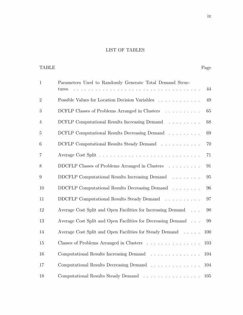
LIST OF TABLES

TABLE Page

1 Parameters Used to Randomly Generate Total Demand Struc-

tures . . . . . . . . . . . . . . . . . . . . . . . . . . . . . . . . . . . 44

2 Possible Values for Location Decision Variables . . . . . . . . . . . . 49

3 DCFLP Classes of Problems Arranged in Clusters . . . . . . . . . . 65

4 DCFLP Computational Results Increasing Demand . . . . . . . . . 68

5 DCFLP Computational Results Decreasing Demand . . . . . . . . . 69

6 DCFLP Computational Results Steady Demand . . . . . . . . . . . 70

7 Average Cost Split . . . . . . . . . . . . . . . . . . . . . . . . . . . . 71

8 DDCFLP Classes of Problems Arranged in Clusters . . . . . . . . . 91

9 DDCFLP Computational Results Increasing Demand . . . . . . . . 95

10 DDCFLP Computational Results Decreasing Demand . . . . . . . . 96

11 DDCFLP Computational Results Steady Demand . . . . . . . . . . 97

12 Average Cost Split and Open Facilities for Increasing Demand . . . 98

13 Average Cost Split and Open Facilities for Decreasing Demand . . . 99

14 Average Cost Split and Open Facilities for Steady Demand . . . . . 100

15 Classes of Problems Arranged in Clusters . . . . . . . . . . . . . . . 103

16 Computational Results Increasing Demand . . . . . . . . . . . . . . 104

17 Computational Results Decreasing Demand . . . . . . . . . . . . . . 104

18 Computational Results Steady Demand . . . . . . . . . . . . . . . . 105

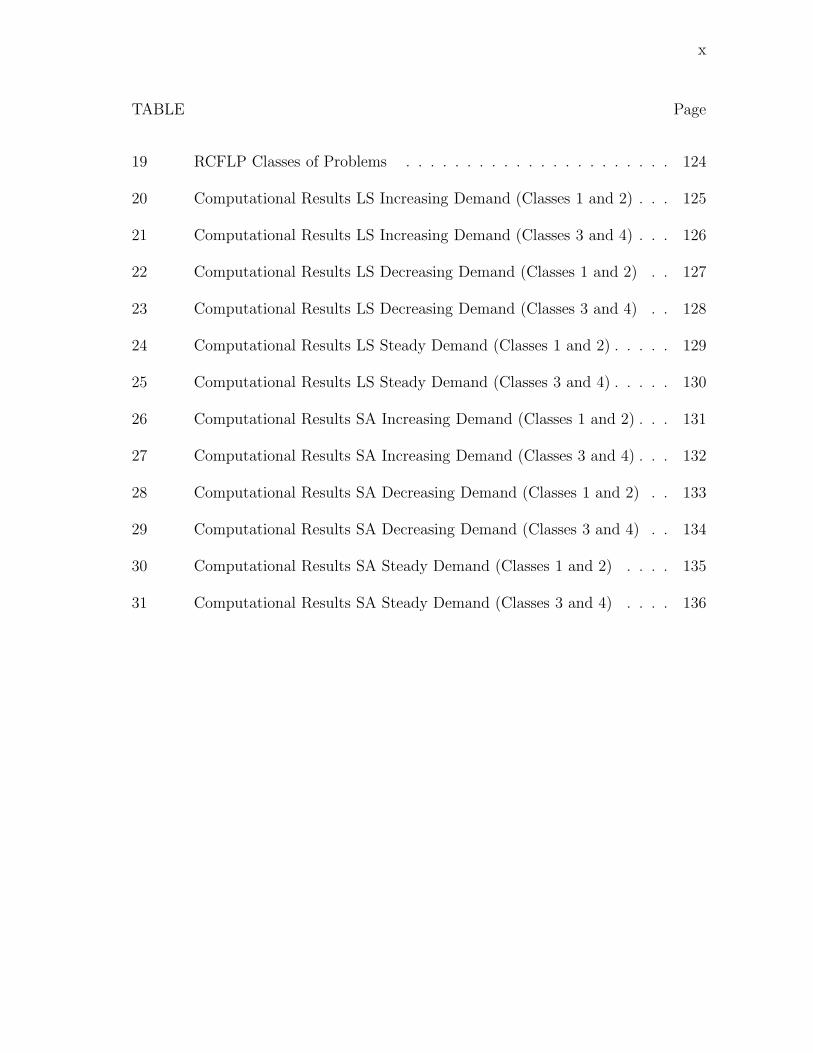
x

TABLE Page

19 RCFLP Classes of Problems . . . . . . . . . . . . . . . . . . . . . . 124

20 Computational Results LS Increasing Demand (Classes 1 and 2) . . . 125

21 Computational Results LS Increasing Demand (Classes 3 and 4) . . . 126

22 Computational Results LS Decreasing Demand (Classes 1 and 2) . . 127

23 Computational Results LS Decreasing Demand (Classes 3 and 4) . . 128

24 Computational Results LS Steady Demand (Classes 1 and 2) . . . . . 129

25 Computational Results LS Steady Demand (Classes 3 and 4) . . . . . 130

26 Computational Results SA Increasing Demand (Classes 1 and 2) . . . 131

27 Computational Results SA Increasing Demand (Classes 3 and 4) . . . 132

28 Computational Results SA Decreasing Demand (Classes 1 and 2) . . 133

29 Computational Results SA Decreasing Demand (Classes 3 and 4) . . 134

30 Computational Results SA Steady Demand (Classes 1 and 2) . . . . 135

31 Computational Results SA Steady Demand (Classes 3 and 4) . . . . 136

xi

LIST OF FIGURES

FIGURE Page

1 Ranges for Slope . . . . . . . . . . . . . . . . . . . . . . . . . . . . . 34

2 Slope Value of Instances with Total Increasing Demand . . . . . . . 35

3 Slope Value of Instances with Total Decreasing Demand . . . . . . . 35

4 Slope Value of Instances with Total Steady Demand . . . . . . . . . 36

5 Customer Locations . . . . . . . . . . . . . . . . . . . . . . . . . . . 37

6 Customer Locations by Region . . . . . . . . . . . . . . . . . . . . . 37

7 Total Demand by Region and Time Period . . . . . . . . . . . . . . 38

8 Customer Demands by Time and Region Total Increasing Demand . 39

9 Customer Demands by Time and Region Total Decreasing De-

mand . . . . . . . . . . . . . . . . . . . . . . . . . . . . . . . . . . . 40

10 Customer Demands by Time and Region Total Steady Demand . . . 41

11 Average Solution Time Increasing Demand (Clusters 1 to 6) . . . . . 73

12 Average Solution Time Increasing Demand (Clusters 7 to 12) . . . . 74

13 Average Solution Time Decreasing Demand (Clusters 1 to 6) . . . . . 76

14 Average Solution Time Decreasing Demand (Clusters 7 to 12) . . . . 77

15 Average Solution Time Steady Demand (Clusters 1 to 6) . . . . . . . 78

16 Average Solution Time Steady Demand (Clusters 7 to 12) . . . . . . 79

1

CHAPTER I

INTRODUCTION

In general, facility location problems deal with the decisions of where to optimally

locate facilities (factories, distribution centers, warehouses, schools, hospitals, etc.)

and how to allocate customers to facilities such that the demand for some service or

product is satisfied. Usually, these decisions are made by considering the associated

costs (or profits) of satisfying the demand and the costs related to establishing (or

operating) the facilities.

The conventional facility location models available in the literature assume that

demand and costs are known and do not change by time. Once the facilities have

been optimally located, they are assumed to remain sited regardless of how demand

and costs may change in future periods. For this reason, the conventional location

models are also called single-period or static location models. In practice, however,

demand is unknown and is time varying. Also, the transportation and operation costs

may increase or decrease from one period to another.

If the total demand for a given product or service is time varying, it might be

necessary to relocate the facilities to meet the upcoming changes. An increase in the

total demand for a given period may require opening new facilities, increasing the

total capacity available to meet the additional demand and to reduce the associated

transportation costs at the expense of opening and operation costs. Similarly, a

decrease in the total demand in any given period may lead to the closure of some

existing facilities to obtain savings on facility operation costs at the expense of the

associated closing costs.

This dissertation follows the style and format of Operations Research.

2

The static location models can not provide an optimal configuration of facilities

when demand is time varying. Observe that relocating the facilities in response to

changes in the total demand can lead to a reduction in transportation costs. Several

models have been developed in the literature to overcome this limitation; they are

known as dynamic location models. Dynamic location models assume that demand

and cost parameters are time varying. Over a given time horizon, they determine

the optimal time and location of facilities in order to minimize the total costs (or

maximize the total profits) for serving demand and for operating and relocating the

facilities.

In some practical situations, the relocation of facilities may not be possible due

to budget constraints. Such situations may arise in the public or private sectors where

facilities like power plants, hospitals, schools, etc. are expected to be operating for

a long period of time. Assuming that the total demand is time varying, a possible

strategy is to determine a fixed configuration of facilities which will remain operational

over the entire time horizon. This configuration should meet the time varying demand

while minimizing the total transportation and operation costs over the entire time

horizon.

When relocation is not allowed, another possible approach is to determine a

robust configuration of facilities such that no matter the value of the parameters in

future periods, the total cost will remain as low as possible. Observe that, in the

absence of relocation costs, the best approach to follow is to use the static (single-

period) location models and optimally determine the locations of facilities for each

period on the time horizon. However, if relocation is not allowed, we can determine a

robust configuration of facilities by minimizing the maximum difference (or deviation)

in total cost between the robust configuration and the optimal configuration for each

time period.

3

In this dissertation, we present mathematical models for dynamic and robust

capacitated facility location problems in time varying demand environments. The

dynamic location model considers the problem of finding the locations of facilities

with limited capacity to satisfy the demand from a set of customers over a discrete

and finite time horizon. The total demand for a single product is assumed to be

time varying in a known way. There are fixed charges (or costs) associated with

establishing (or opening) new facilities, operating existing facilities, and for closing

existing facilities. Also, there is a transportation cost for serving the demand of

customers from open facilities. The main objective of the model is to determine

an optimal sequence for locating facilities to satisfy the time varying demand while

observing the capacity restrictions over the time horizon. We denote this problem as

Dynamic Capacitated Fixed Charge Location Problem (DCFLP).

We also present two location models considering a similar problem setting as in

the DCFLP but without relocation of facilities. The first model determines a fixed

configuration of facilities that minimizes the total costs for opening and operating

facilities and for shipping demand from facilities to customers over the entire time

horizon. We denote this problem as Dynamic Demand Capacitated Fixed Charge

Location Problem without relocation (DDCFLP). In Chapter IV, we show that when

relocation costs are considerably large, the DDCFLP can be solved by the DCFLP

model as a special case.

The second model considers the problem of finding a configuration of facilities

that minimizes the maximum regret or difference in total cost with respect to the

optimal solution for each time period. We denote this problem as Robust Capacitated

Fixed Charge Location Problem (RCFLP).

4

I.1. Research Contributions

The conventional facility location models ignore the time varying behavior of demand

and cost parameters, regardless of how long the facilities are expected to remain

operational. The dynamic and robust location models in this dissertation address

this limitation by incorporating strategic decisions for locating facilities throughout

the time horizon. In particular, we contribute to the literature in facility location as

follows.

1. We develop a mathematical model for the DCFLP to determine the optimal

time and location for establishing capacitated facilities (as well as the allocation

of customers to facilities) in order to minimize the total cost, when demand

and cost parameters are time varying. We present a Lagrangian relaxation-

based algorithm as well as a Benders’ decomposition framework to solve the

model. The efficiency of the solution methods depends on the structure of

the problem and characteristics of the input data. The Lagrangian relaxation

algorithm shows to be efficient in solving problems where the expected number

of open facilities is small, and the total fixed operation cost accounts for more

than half the objective function value. The Benders’ decomposition algorithm

demonstrates to be efficient for problems with a large number of expected open

facilities, and significantly more efficient when the total fixed operation cost

represents the major portion of the objective function value.

2. We develop a mathematical model for the DDCFLP. The model determines

a fixed configuration of facilities that minimizes the total cost when demand

and cost parameters are time varying. We present a Benders’ decomposition

algorithm to solve this model.

5

3. We develop a mathematical model for the RCFLP. The model determines a ro-

bust configuration of facilities that minimizes the maximum difference in terms

of total cost with respect to the optimal solution for each time period. We

implement Local Search and Simulated Annealing metaheuristics to solve this

model.

4. We conduct an empirical analysis that gives strategic insights for decision mak-

ers when dealing with location problems when the total demand is time varying,

in a known way, and following an increasing, decreasing, or steady pattern.

I.2. Organization of the Dissertation

The remainder of this dissertation is organized as follows. In Chapter II, we present

a review of the literature on dynamic and robust facility location. In Chapter III, we

describe the characteristics of the time varying demand structures and the generation

of random data for experimentation. In Chapter IV, we formulate and solve the

DCFLP model and present an empirical analysis of the solution methods. In Chapter

V, we present the formulation of the DDCFLP model and the solution approach. We

show that when relocation costs are considerably large, this problem can be solved

as a special case by the DCFLP model. In Chapter VI, we formulate the RCFLP

model, discuss the solution methodology, and present computational results. Finally,

in Chapter VII, we present conclusions and discuss areas of future research.

6

CHAPTER II

LITERATURE REVIEW

II.1. Introduction

In general, facility location problems can be classified into two groups: continuous

and discrete location problems. Continuous (or planar) location problems consider

the location of demand or customers and new facilities to be at any point on the

plane. Distances between points are generally represented by norms. The �p norm

is a commonly used norm for distance representation (Love et al., 1988); its special

forms include p = 2 (Euclidean distance) and p = 1 (rectangular distance). On the

other hand, discrete location problems consider the location of demand and facilities

on the nodes and links of a graph or network (usually only at the nodes); the travel

distances between demand points and facilities are represented by the arcs of the

network. Complete surveys of facility location problems are provided by Brandeau

and Chiu (1989), Francis and Mirchandani (1990), Drezner (1995b), Owen and Daskin

(1998), and Drezner and Hamacher (2002).

The minisum and minimax location problems are classic location problems that

have been formulated as continuous or discrete location models. The minisum prob-

lem has the objective of finding the location of a single or multiple facilities in such

a way that the weighted Euclidean distances from a fixed number of points to the

facilities are minimum. In the minimax problem, the objective is to determine the

location of facilities such that the maximum distance from a set of points to the new

facilities is minimum.

The classification of location problems can be further extended to consider cer-

tainty or uncertainty in the parameters. In certainty situations, the value of the

7

parameters is assumed to be known. In uncertainty situations the value of the param-

eters in the future is unknown and several possible realizations or scenarios need to be

considered. Location problems in uncertainty can be stochastic or robust. Stochastic

location problems consider a probability distribution associated with each possible

realization or scenario. In robust location problems, no probability distribution in-

formation is available and a set of possible scenarios needs to be considered. The

main objective of robust location problems is to find the location of facilities that will

have a good performance (cost wise) under future changes in the value of uncertain

parameters. Common robustness measures used in the literature consider minimizing

the maximum cost, minimizing the worst-case cost (or regret), and minimizing the

maximum relative regret (or relative deviation) (Kouvelis and Yu, 1997).

In this dissertation, our main focus is on dynamic and robust location models.

We assume discrete locations for facilities and customers. The demand and cost

parameters are assumed to be changing by time in a known way. Thus, our location

models are discrete and deterministic.

This chapter is divided into two main sections. In Section II.2, we review the

literature in dynamic facility location. In Section II.2.2, we review the literature

in robust facility location with special focus on solution strategies applicable to our

robust location model. In Section II.4, we describe the position of this dissertation in

the current literature. Finally, in Section II.4, we present a summary of the chapter.

Throughout this chapter we assume the reader is familiar with continuous and

discrete location models. The interested reader is referred to Love et al. (1988),

Drezner (1995b) or Daskin (1995) for an introduction to location theory.

8

II.2. Dynamic Facility Location

Dynamic facility location models can be considered to be extensions of the conven-

tional (single-period or static) models as they include time varying demand. Most

of the models developed in the literature for dynamic location problems assume that

facilities can be relocated between periods in response to changes in demand. There

are associated relocation costs for changing the location of facilities between periods,

which can represent the initial investment for establishing new facilities and the cost

(or savings) for the closure of existing facilities.

Most of the continuous and discrete static location problems are known to be

NP-hard. Dynamic location problems are at least as difficult to solve as the static

problems due to the additional consideration of time. However, the algorithms and

solution approaches developed for static location problems can be adapted to solve the

dynamic problems. Throughout this section we review the literature in dynamic facil-

ity location. We separate the dynamic models into continuous and discrete location

models.

II.2.1. Continuous Location Models

Perhaps the first model that considers time varying demand and relocation of facilities

is given by Ballou (1968). The dynamic location/relocation model considers a single

warehouse where the objective is to maximize the total net profit along a finite and

discrete planning horizon. The model is solved using the recursion formula of discrete

dynamic programming (Bellman, 1966). The set of candidate locations for facilities

is constructed from the optimal solutions of the static warehouse location problem

for each period. This is a restriction on the dynamic programming procedure to work

only with a fixed state space of alternative locations for each period. A drawback of

9

this solution approach is that the set of candidate locations may exclude potential

sites that can increase the maximum profit for the overall problem. Therefore, this

approach can be considered to be a heuristic solution method.

A different type of problem is given by Scott (1971), introducing two different

models for the single facility dynamic location-allocation problem. In this problem a

single facility is to be located at the beginning of each period of a finite and discrete

time horizon. It is assumed that the number of customers and facility locations are

stationary and the transportation cost remains constant in subsequent periods after

the end of the time horizon. The first model considers a myopic optimization process

which does not anticipate the future. The minimum cost location of a single facility is

determined only for the current time period, considering the existing (sited) facilities

at that time, and continues in this fashion until the last facility is located. The

second model uses dynamic programming to determine the over-all optimum taking

into account future events. The recursion formula of discrete dynamic programming

is used to determine the complete sequencing of the facility construction plan that

minimizes the cumulative cost.

Wesolowsky (1973) presents a general multi-period formulation of the Weber

problem (Weber and Friedrich, 1929). This dynamic formulation allows changes in

the location of a single facility along a finite planning horizon. The demand, number

of destinations (demand points), and the associated costs for serving demand and

relocating the facility are assumed to be time varying. A dynamic programming

algorithm is used to optimize the sequence of locations in order to meet changes

in costs, volumes, and locations of destinations. The procedure is represented by a

decision tree where each node represents a sequence of configurations for each time

period, allowing the elimination of duplicated solutions. This incomplete dynamic

programming algorithm reduces the number of static problems to be computed more

10

than using complete enumeration. This algorithm is an optimal solution method for

the problem presented by Ballou (1968).

In a subsequent paper, Wesolowsky and Truscott (1976) propose a dynamic

multi-facility minisum problem. The model can be considered to be a reformulation

of the previous model introduced by Wesolowsky (1973), by allowing the establish-

ment of new facilities and the removal of both existing and new facilities within the

planning horizon. In this formulation, the locations for a fixed number of facilities are

assumed to be at any place on the plane. Changes in location, in response to changes

in demands and costs, are permitted with an associated relocation cost. A segmented

bounded algorithm is developed to solve the problem. The algorithm solves a series of

static minisum problems, corresponding to segments of a binary matrix, and selects

the least cost solution. This binary matrix specifies the movements of facilities along

the planning horizon. Using this approach the total number of static problems to be

solved is reduced considerably compared to using a complete enumeration approach.

Megiddo (1986) considers two types of dynamic 1-center problems: global opti-

mization and steady-state. Demand points are assumed to be moving (or changing

location) according to a linear function over the time horizon. The global optimiza-

tion problem looks for a point in time when the solution to the static 1-center problem

yields the best solution for all time periods. In the steady-state problem the objective

is to determine the steady-state behavior of the system, i.e., a point in time when

the location of the facility or center will remain unchanged in the following periods.

The dynamic 1-center problem in the plane is used to solve both problems. Solution

algorithms for the static 1-center problem are adapted to solve these dynamic location

problems.

Drezner and Wesolowsky (1991) study the problem of locating a facility among

a given set of demand points when the weights associated with each demand point

11

change in time in a known way, and the location of the facility is allowed to change

one or more times during the time horizon. The weight associated with each demand

point is assumed to be a continuous function of time. The problem is to find the

time breaks when the location of the facility must be changed as well as its location

during the time span between breaks. Both minisum and minimax formulations are

considered as dynamic location problems. The solution algorithm for the minisum

problem considers rectangular distances; it scans all possible break points that can

be optimal and selects the best. To solve the minimax problem, two algorithms are

given using bisection search and considering Euclidean distances.

Drezner (1995a) presents a formulation of the dynamic p-median problem when

demand is changing over time and new facilities are built at given times. This problem

is called progressive p-median problem, since new facilities or medians are established

sequentially in each period. The solution approach for the problem is derived using a

numerical example. In this example, two new facilities are to be located considering

Euclidean distances. This problem is solved by a special algorithm, similar to the

2-median problem given by Drezner (1984). The general problem is solved using

standard nonlinear mathematical programming code. This type of p-median problem

arises in situations where demand is increasing over time in a known way, such that

new facilities need to be established sequentially at given time periods.

II.2.2. Discrete Location Models

The literature available in discrete dynamic location problems is considerably richer

than continuous models. Usually, discrete location problems are formulated as integer

or mixed integer programs and solved using the optimization methods developed for

this type of mathematical models.

The restriction of facility locations to the nodes of a network is considered by

12

Erlenkotter (1974), introducing a network-based model for the single facility location

problem. Each discrete time period in the planning horizon is represented by a node.

The arcs of the network denote the relocation and operation costs of the facility be-

tween time periods. The optimal solution is obtained recursively by evaluating the

minimum location policy cost discounted to time period over the time span between

the periods at which the facility is relocated. This network solution approach is equiv-

alent to the incomplete dynamic programming algorithm presented by Wesolowsky

(1973) with discrete locations.

Kolesar and Walker (1974) present an application of the dynamic set covering

location problem to the relocation of fire companies in New York City. The problem

is divided into several stages and solved sequentially to determine the relocation plan

that gives a coverage with minimum response time. This procedure considers the

solution of a series of linear integer programs. A heuristic algorithm and a computer-

based program are proposed to determine the best relocation plan.

A special type of p-median problem is presented by Wesolowsky and Truscott

(1975). The model considers the multi-period discrete space location-allocation prob-

lem. The purpose of this model is to devise a plan of optimal locations and relocations

in response to predicted changes in the demand volume originating at demand points

over a finite planning horizon. The model is solved using a dynamic programming

algorithm with backward recursion for small size problems.

Roodman and Schwarz (1975) give a dynamic model for the uncapacitated facil-

ity location problem. This formulation determines the time at which a set of initially

open facilities are to be closed. Once a facility is closed it can not be reopened. This

situation arises when demand is decreasing over the time horizon and facilities are

supposed to be closed sequentially in each time period. The problem is solved by

exploiting the special economic structure of the problem. The algorithm consists of

13

partial assignments of customers to facilities and a modified branch and bound proce-

dure, similar to the branching rules method given by Efroymson and Ray (1966) and

Khumawala (1972). Also, a heuristic procedure is used together with the branching

rules to obtain approximate optimal solutions.

Revelle et al. (1976) study a multi-period extension of the set covering problem.

In this formulation it is assumed that the set of customers at each time period is a

subset of the next period. The set of potential locations for facilities remains the same

in each period of the planning horizon. The location pattern over time is obtained

by solving the static set covering problem. Facilities are located only when they

are required. A disadvantage of this model is that after the solution is obtained, a

secondary procedure is required to find the time-phasing of facilities.

Sweeney and Tatham (1976) propose an improved model for solving the multi-

period multiple warehouse location problem with opening and closing of capacitated

facilities. This type of location problem was first discussed by Ballou (1968). The

improved model integrates the mixed integer program formulation of the single ware-

house location problem with a dynamic programming procedure for finding the opti-

mal sequence of configurations over multiple periods. It is shown that only the best

ranked-order solutions (ranked in nondecreasing order of the objective function value)

in any single period need to be considered as candidates in the optimal multi-period

solution. This consideration reduces the state space of the dynamic programming

algorithm in a similar way to the solution approach given by Wesolowsky (1973).

Schilling (1980) presents an application of the dynamic maximum covering lo-

cation problem for establishing emergency services. The mixed integer program for-

mulation is an extension of the static maximum covering problem. This formulation

requires that a certain number of facilities must be open at each period. In this

model, the objective function is represented as a vector with the multiple objectives

14

of maximizing the coverage in each period. The model is solved using a heuristic

myopic procedure that evaluates alternative configurations between successive peri-

ods as long as the maximum coverage is improved. This heuristic is combined with a

weighting method to evaluate dominating solutions for the problem.

Erlenkotter (1981) presents a comparison of seven approximate methods for a dy-

namic model of the CFLP considering both discrete-time and continuous-time frame-

works. The general problem is to locate new capacity over time to minimize the total

discounted costs of meeting growing demand at several locations. Due to the level

of complexity of the problem, the use of mixed integer programming optimization

methods does not guarantee that the optimal solution for practical size problems is

obtained. Two industrial problems given by Manne (1967) are used to test the perfor-

mance of these seven heuristic methods. The comparative results show that the type

of formulation using discrete or continuous time affects the form of the solution. For

discrete-time formulations the solutions tend to force the capacity expansions into

multiples of individual period demand increments. In continuous-time formulations

there is more flexibility to choose the size and restrictions of the capacity expan-

sion. Concluding remarks point out that improved results can be obtained using a

combination of the heuristic solution methods.

Chrissis et al. (1982) present a dynamic version of the set covering problem that

considers the phase-in/phase-out cost of facilities. The model considers the facility

operation and relocation costs. To determine the penalties or cost due to relocation,

a logic constraint is added to the model. The objective of this model is to minimize

the total number of facilities required to cover all the demand points over all time

periods. The model is solved using an approximation algorithm.

Gunawardane (1982) introduces dynamic formulations of the set covering and

maximum covering problems considering the phase-in/phase-out of facilities. The

15

dynamic set covering formulation is based on the model discussed by Revelle et al.

(1976). Since the dynamic model has the same number of constraints but more vari-

ables than the static set covering model, the solution procedure considers the linear

programming relaxation. The optimal solutions obtained for a set of test problems

display the integrality property. The dynamic formulation is extended to consider the

individual cases of phase-in and phase-out of facilities. A shortcoming of the proposed

dynamic formulations is that for practical size problems the integral solution of the

linear programming relaxation is not guaranteed.

Van Roy and Erlenkotter (1982) study a dynamic location model similar to the

model introduced by Roodman and Schwarz (1977). This model prevents the reloca-

tion of facilities, that is, opening a new facility at the most once and closing an initially

existing facility at the most once. The solution method, denoted as DYNALOC, is

a dual-based algorithm combined with a primal-dual adjustment procedure and a

branch and bound algorithm. This solution approach is a modified version of the

DUALOC procedure proposed by Erlenkotter (1978) for the static uncapacitated fa-

cility location problem.

An application of the solution approach proposed by Sweeney and Tatham (1976)

is given by Kilmer et al. (1983). The purpose of this study is to determine the ad-

justments over time required in number, size, and location of citrus packing-houses in

east Florida. It is assumed that the volume and location of production is changing by

time. The mixed integer programming formulation does not consider opening/closing

costs for facilities. Each single period problem is solved using a search code proce-

dure. A dynamic programming algorithm is used to find the path adjustments of

packing-houses over the planning horizon and to obtain the optimal configuration.

A different approach for the dynamic location problem is proposed by Kelly

and Marucheck (1984). The problem considers that the optimal decision to open or

16

close a facility at a given point in time would become suboptimal when the planning

horizon is extended or when the problem parameters change in subsequent periods.

The mixed integer programming model determines the set of warehouse locations

for each time period of a finite time horizon. This model incorporates the facility

operation, opening, and closing costs. The solution methodology consists of obtaining

a partial optimal solution by a bounding procedure similar to the delta and omega

tests proposed by Efroymson and Ray (1966) and Khumawala (1972). The reduced

model is then solved using Benders’ decomposition. An optimal solution is later

examined to determine if post horizon conditions could affect the location decisions.

The purpose of this model is to determine the optimum relocation plan of facilities

considering post-horizon conditions.

Chand (1988) considers the single facility location/relocation problem in an in-

finite time horizon. The location/relocation decisions are defined under the concepts

of decision horizons/forecast horizons (DH/FH), i.e., the length of time where initial

location decisions are to be taken (DH), and the number of time periods of forecasted

data (FH) needed to make such decisions. The main objective is to determine the

minimum number of periods needed to optimally define the DH as well as the FH

for an infinite time horizon. A forward dynamic programming algorithm is developed

to determine the optimal initial decisions within a finite horizon to determine the

optimal location of a single facility.

Frantzeskakis and Watson-Gandy (1989) consider the problem of finding a lo-

cation plan over a planning horizon, which selects the location of facilities in each

period in such a way that the total costs of transportation, operation, and reloca-

tion are minimized. The problem is formulated as a dynamic program, restricting

the number of open facilities in each period. The problem is solved using dynamic

programming and a branch and bound procedure with state space relaxation.

17

Hakimi et al. (1999) study the 1-median and k-median problems on a time varying

or dynamic network. Time is considered a discrete variable and the parameters of

the network (demands at the vertices and lengths of the arcs) are known functions

of time. The location of the facility during each time period can be a point along

some edge on the network; this choice may or may not change in the next period.

The 1-median problem is to find the locations of the facility along the time horizon

that minimizes the cost of servicing demand and relocating the facility. The dynamic

k-median problem is defined in a similar way but to find the locations of k facilities

on the dynamic network. The dynamic 1-median problem can be solved using an

augmented graph, computing the shortest path between locations. The k-median

problem can be solved in a similar way by successively solving the problem for each

time period and finding the k locations that minimize the total cost.

The problem of capacity expansion and dynamic plant location is presented by

Shulman (1991). This class of dynamic capacitated location problem considers differ-

ent types of facilities with finite capacities. The objective is to find the optimal facility

expansions (or mix of facilities) at each location when more than one facility can be

placed at a given location. The problem is formulated as a mixed integer program.

This formulation is solved using Lagrangian relaxation of the capacity constraints.

This type of relaxation simplifies the problem into small optimization subproblems,

one for each candidate facility location. These subproblems are solved for fixed values

of Lagrangian multipliers using dynamic programming. Two solution algorithms are

designed. The first solves the general dynamic problem considering different types

of facilities. The complexity of this algorithm is exponential in the number of facil-

ities and may be used only for small problems. The second algorithm considers the

case where different types of facilities can not be located at the same location. This

algorithm has a polynomial complexity and can be used for large problems.

18

Bastian and Volkmer (1992) study a similar problem considered by Chand (1988).

A perfect forward procedure is developed to determine the optimal initial decision by

using only information from the smallest forecast horizon. Given an infinite planning

horizon problem, it may be possible to find the optimal initial decision by using only

information from a finite number of periods. The fixed cost of relocating the facility

may depend on the period as well as the locations. The solution algorithm uses the

data structure of a policy tree which is adapted from the lot tree approach for solving

dynamic lot size problems.

Most of the dynamic location models consider the planning horizon as an ex-

ogenous input. Daskin et al. (1992) consider a dynamic location model in which the

objective is to find a planning horizon (optimal forecast horizon) and a first period

decision (optimal initial decision) such that the conditions after the planning horizon

do not influence the choice of the optimal initial decision. This approach suggests that

the planning horizon for a dynamic location problem should be determined endoge-

nously. Using an empirical approach it can be determined whether or not forecast

horizons are likely to exist. The concepts of ε-optimal forecast horizon and the ε-

optimal initial decision are introduced. For given empirical tests, it is shown that

good initial decisions and empirical ε-optimal forecast horizons could be found for

small size problems.

Andreatta and Mason (1994) present a note regarding the work of Bastian and

Volkmer (1992). This note refers to the previous work of Chand (1988) about

the perfect forward algorithm for the solution of the single facility dynamic loca-

tion/relocation problem. A numerical example is solved to demonstrate that this

problem does not always have a finite forecast horizon. The perfect algorithm that is

presented differs from the policy trees proposed by Bastian and Volkmer (1992) and

the regeneration sets used by Chand (1988). Instead, this algorithm uses all possible

19

ending states. This approach can be viewed as a modified version of the Dijkstra’s

algorithm.

Chardaire et al. (1996) give a quadratic programming formulation for the dy-

namic uncapacitated facility location problem. The model is solved using Lagrangian

relaxation and Simulated Annealing. The Lagrangian subproblem is solved using dy-

namic programming to optimality. The set of open facilities is given as an input to

Simulated Annealing to find a good feasible solution. It is shown that the bound

obtained by the Lagrangian dual is equal to the bound obtained from the linear

programming relaxation of the linearization of the quadratic model.

Location problems can be extended to the case where facilities can be established

in different geographic regions and operate under different economic environments.

Canel and Khumawala (1996) present mixed integer programming formulations for

the capacitated and uncapacitated multi-period international facility location problem

(IFLP). This class of location problem is similar in purpose to the location model

studied by Rıos-Ramırez (2003). In addition, the IFLP incorporates the quantitative

characteristics of locating facilities in foreign countries and the economic implications.

These economic considerations include factors such as international customers and

competition, market access and proximity, lower labor costs, economies of scale, taxes,

incentives, inflation rates, and so on. The IFLP arises in situations where companies

respond to the external environment and seek advantage available at international

locations. The objective of the multi-period IFLP is to determine in which countries

to locate facilities, the timing for the location decisions, and the quantities to be

produced and shipped to the customers such that either total costs are minimized

or total after-tax profits are maximized. The structure of the model considers the

existence of a domestic plant and facilities that can be located in foreign countries to

supply the demand of customers in a global market. Both mixed integer programming

20

formulations are compared with an actual company case given in the literature. The

models are solved using standard optimization software. Also, a sensitivity analysis

is conducted to evaluate alternative plans for the problem.

Hormozi and Khumawala (1996) give an exact algorithm for the multi-period

facility location problem. The mixed integer programming formulation corresponds

to the multi-period, multi-stage facility location problem, incorporating opening and

closing costs for facilities. The model considers a set of plants with limited capac-

ity that can serve customers and facilities. The solution algorithm is based on the

method presented by Sweeney and Tatham (1976) and provides an improvement over

this procedure by reducing the computational requirements. Two simplification pro-

cedures are introduced to reduce the size of the general facility location problem

(improved lower bound and delta/omega augmentation). This algorithm considers a

rank-ordered number of solutions to static problems for each period of the planning

horizon. Dynamic programming is used to obtain the optimal sequence of facility con-

figurations that minimizes the total cost. The reduction techniques reduce the number

of single period problems that need to be considered by the dynamic programming

part. The proposed improved algorithm required fewer single period problems and

took less computational time when tested and compared to the procedure of Sweeney

and Tatham (1976).

Canel and Khumawala (1997) propose a branch and bound algorithm to solve

the multi-period IFLP. The mixed integer programming formulation incorporates

quantitative factors such as demand, investment cost, manufacturing and labor costs,

transportation and transfer costs, taxes and tariffs, exchange rates, plant equipment

and fixed costs. The proper calculation of the relevant costs impact the efficacy of

the model. The branch and bound algorithm uses the simplifications and branching

rules given by Khumawala (1972) and Hormozi and Khumawala (1996). Using the

21

data from the previous case of study (Canel and Khumawala, 1996), the formulation

is solved for uncapacitated and capacitated problems using the branch and bound

algorithm.

Saldanha da Gama and Captivo (1998) give a discrete dynamic formulation for

the uncapacitated fixed charge location problem (UFLP) that considers fixed costs

for operating, opening, and closing facilities. Opening/closing of facilities is limited

to take place at most once for each period except for the last period of the time

horizon. The model is solved using a two-phase heuristic. The first phase consists of

a modification of the drop procedure introduced by Kuehn and Hamburger (1963).

The procedure begins with all facilities open for all periods and iteratively takes

out periods in the operation of some facility until no further elimination is possible

without losing feasibility. In the second phase, local search is applied using a radius-

k neighborhood with k = 1. The neighborhood of a feasible solution is defined as

the set of different feasible solutions with the addition or removal of no more than k

operation periods in some facility. The purpose of local search is to adjust the initial

feasible solution obtained in the drop phase. To test and compare the performance

of the two-phase heuristic a computational experiment is presented. A comparison

between the heuristic method and the solution approach proposed by Van Roy and

Erlenkotter (1982) showed that the heuristic obtained good results in computing time

and solution quality.

Canel and Das (1999) consider the multi-period facility location problem with

profit maximization. The objective function considers the fixed and investment costs

for locating facilities, transfer and manufacturing costs for transportation charges,

and the revenue for sent quantities from facilities to customers. The mixed inte-

ger programming formulation is solved using an implementation of the branch and

bound algorithm and simplification rules given by Efroymson and Ray (1966) and

22

Khumawala (1972). For a series of test problems, the results obtained showed that

the proposed algorithm is efficient in obtaining optimal solutions in short time when

compared with standard optimization software.

In a research report given by Dias et al. (2001a), three types of dynamic ca-

pacitated location problems with opening, closure, and reopening of facilities are

presented. The first type of problem considers facilities with a maximum capacity at

the opening period. This maximum capacity remains constant during the operating

time of the facility. The second problem considers a maximum and minimum ca-

pacity for facilities. The third problem considers facilities with maximum decreasing

capacity at the opening period or a maximum expansion at the reopening period. It

is assumed that capacity decreases as customers are assigned to the facility. For this

third problem, the possibility for a facility to be closed even if its available capacity

has not been depleted is considered. If this facility is reopened in a subsequent pe-

riod it will, in addition, have its remaining capacity from when it was closed. For

each type of problem a mixed integer program and its associated dual formulation are

given. Primal-dual heuristics are used to solve each type of problem. These heuristics

are based on the work of Erlenkotter (1978) and Guignard-Spielberg and Spielberg

(1977). The procedure uses a dual ascend, dual adjustment, a primal procedure, and

dual descent procedure for each dual variable. A numerical example is solved for each

problem to illustrate the performance of the heuristics.

Dias et al. (2001b) present a hybrid heuristic algorithm to solve capacitated and

uncapacitated dynamic location problems. This research report considers the model

previously discussed by Dias et al. (2001a). The formulation of a general mixed in-

teger programming model is extended to consider opening, closing, and reopening of

four types of facilities: uncapacitated facilities, facilities with maximum and/or min-

imum capacity, facilities with maximum decreasing capacity, and facilities composed

23

of one or more elements of different dimensions (capacities). The general formula-

tion is also extended to consider additional restrictions and multi-objectives. The

heuristic solution method integrates genetic algorithm with local search. The genetic

algorithm phase works with the generation, diversification, and evolution of solutions

(individuals). A binary matrix is used to represent the opening, closing, and re-

opening of facilities in each time period (chromosomes). The genetic operators used

are selection (binary tournament), crossover (adaptation of one-point crossover), and

mutation (probabilistic). The local search phase works with one solution at a time

to improve its fitness (objective function value) by searching k-neighborhoods. A

k-neighborhood consists of different solutions obtained by inserting or extracting k

operating periods to a facility. The genetic algorithm considers a random initial con-

figuration of open facilities (population) and generational replacement with elitism.

This hybrid algorithm is extended to include additional restrictions or multi-objectives

in the formulation.

Dias et al. (2004a) develop a model for dynamic location problems with discrete

expansion and reduction sizes of capacity. This model is similar to the model given by

Shulman (1991), since facilities of equal or different capacities can be established at

the same location. In addition, this model considers opening, closing, and reopening

of facilities more than once along the planning horizon. The mixed integer program-

ming formulation is similar to the model presented by Dias et al. (2001a) (maximum

capacity case). However, the model is adapted to consider facilities with different

discrete capacities. The primal-dual heuristic is very similar to the solution approach

previously discussed by Dias et al. (2001a). The concluding remarks mention that the

results obtained using this approach can be improved by incorporating local search

for improving the primal solution.

Dias et al. (2004b) extend the application of the primal-dual heuristic proposed

24

by Dias et al. (2001a) to dynamic multi-level capacitated and uncapacitated location

problems. This research report presents mixed integer programming formulations for

several dynamic uncapacitated and capacitated multi-level location problems. These

models consider the possibility of a facility being opened, closed, and reopened more

than once during the planning horizon. Two types of capacity restrictions are con-

sidered, maximum capacity and maximum and minimum capacity but without flow

conservation at the intermediate facilities. For each dynamic multi-level problem a

dual formulation and the complementary conditions are derived to define the primal-

dual procedure (Erlenkotter, 1978).

Balakrishnan (2004) extends the work of Hormozi and Khumawala (1996) by

proposing a pruning rule for the multi-period facility location algorithm. The use

of this rule can reduce the number of single period configurations to be considered

by the dynamic programming algorithm. The same example given by Hormozi and

Khumawala (1996) is solved to illustrate the effectiveness of the pruning rule. Also,

an experiment is conducted to test its general effectiveness. The additional com-

putational effort to implement it is minimal. This type of reduction is possible by

considering each period independently. Separating the material flow cost and the lo-

cation configuration rearrangement cost, some configurations with low material flow

cost within a period can be ignored from consideration in the dynamic programming

algorithm. This occurs if these configurations have a rearrangement cost not greater

than their higher material flow cost.

II.3. Robust Facility Location

As we mentioned before, robust location problems provide solutions with acceptable

results when the future value of parameters is uncertain. Robust location problems

25

can be classified according to characteristics of uncertain parameters, for instance, dis-

crete scenarios are used when no probability distribution is known. The robustness

of a solution represents a measure of a decision under uncertainty. Typical measures

of robustness discussed in the literature include the minimization of the maximum

cost (or minimax), minimum worst-case deviation cost (or minimax regret), and min-

imization of the maximum relative regret (or minimax relative deviation).

To illustrate each one of these robustness measures consider the following nota-

tion. Let x�, � = 1, . . . , k be the decision variables, X the set of feasible solutions,

s ∈ S the possible scenarios, w�s the cost for decision variable � in scenario s, and Z∗s

the optimal total cost for each scenario.

In the minimax approach, the objective is to find a solution for which the maxi-

mum cost over all possible scenarios is minimum:

minx∈X

maxs∈S

k∑�=1

w�sx� (2.1)

In the minimax regret approach, on the other hand, a solution is defined as robust if

it minimizes the maximum difference or deviation over all scenarios with respect to

the optimal solution for each scenario:

minx∈X

maxs∈S

{k∑

�=1

w�sx� − Z∗s

}(2.2)

Finally, the minimax relative regret approach considers the case when the difference

between the robust configuration and the optimal solution for each scenario varies

considerably. Thus, the ratio between the difference or deviation and the optimal

solution for each scenario is used instead:

minx∈X

maxs∈S

{(k∑

�=1

w�sx� − Z∗s

)/Z∗

s

}= min

x∈Xmaxs∈S

{(k∑

�=1

w�sx�/Z∗s

)− 1

}(2.3)

Robust location problems with a minimax objective function are more difficult to solve

26

than problems with minimization (or maximization) objective function and require

higher computational effort. For this reason, most of the models developed in the

literature consider small size problems (usually 1-center or 1-median on a tree).

The literature available in robust facility location is quite recent and scarce,

compared to the literature developed in dynamic facility location. The interested

reader in robust optimization is refereed to the book of Kouvelis and Yu (1997).

Averbakh and Berman (1997) consider a minimax regret p-center problem on a

general network. The weights or demands at the nodes of the network are assumed to

be uncertain. The value of the demands is estimated using an interval. To solve the

problem, a polynomial time algorithm is developed. This algorithm solves n static

p-center problems, one for each node on the original network, and one in an auxiliary

network. For the 1-center problem on a general network and the p-center problem on

a tree, the solution time of the algorithm is shown to be polynomial.

Daskin et al. (1997) study a variant of the minimax regret p-median problem on a

network. In this problem a probability is assigned to each scenario and only a subset

of the scenarios is selected such that the total probability is at least a predefined value,

α. The model minimizes the maximum expected regret over the selected scenarios.

This approach is denoted as α-reliable since the regret of the selected scenarios will

be bounded by the solution obtained from the model. A computational experiment

is performed using commercial optimization software to test the model for different

values of α.

Current et al. (1998) introduce two approaches for the dynamic p-median problem

when the total number of facilities to be located is uncertain (NOFUN). The problem

is analyzed by two different criteria: the minimization of expected opportunity loss

and the minimization of maximum regret. In general, these criteria assume that there

are a finite number of options and a finite number of possible states of nature. For

27

each scenario there is a possible initial configuration of open facilities, each with a

given probability of resulting in the final state configuration. The optimal solution

for the problem may consider the restriction that the initial configuration is a subset

of the final configuration. A solution with minimum expected opportunity loss can be

obtained by solving a binary integer formulation. The solution of NOFUN problems

by the minimax regret criterion does not consider the probabilities for the various

states of nature. The optimal set of open facilities for the initial configuration is

obtained by minimizing the maximum difference between the optimal solution of the

p-median (without the restriction of having the initial configuration in the final state)

for each possible state of nature, and the optimal solution of the p-median (with the

restriction) for each potential state of nature and for each of the potential initial siting

configurations.

Serra and Marianov (1998) present minimax and minimax-regret discrete location

models for the p-median problem when demand and travel times or distance are

uncertain. The application of the models is to locate fire stations in the city of

Barcelona, Spain. Both models consider several possible scenarios to select the set

of locations that will perform well over all future scenarios. The initial solution for

both models is obtained by constructing a matrix with the optimal solutions of the

static p-median for each scenario. The heuristic algorithm proposed for both models

considers an exchange heuristic to improve the initial solution.

Vairaktarakis and Kouvelis (1999) study several formulations for the 1-median

problem on a tree. These formulations consider dynamic change and uncertainty in

the demand and transportation costs over a discrete and finite time horizon. Dynamic

demand at the nodes and transportation costs in the arcs’ length are represented by

linear functions. The uncertainty in demand and transportation cost are represented

by scenarios. The robustness measures considered are minimax regret and relative

28

regret. For all the models a polynomial algorithm is developed.

Averbakh and Berman (2000) consider the 1-center problem on a tree where

the demand or weights at the nodes and the arcs’ lengths are modeled as uncertain

parameters. The value of the uncertain parameters is assumed to be random, with

unknown probability distribution, and is estimated within a given interval. The

objective is to find the location of the center that minimizes the maximum regret

over all possible scenarios. A polynomial time algorithm is developed. For the special

case where the weights are certain and equal for all points, the complexity of the

solution algorithm reduces significantly.

Averbakh (2000) study a group of combinatorial optimization problems with

minimax objective function and uncertain parameters. The methodology to find

minimax regret solutions consists of reducing the problems with uncertainty into a

series of deterministic problems. The solution algorithms for the deterministic prob-

lems are then used to obtain efficient algorithms for the uncertain problems. The

optimization problems solved consider minimax regret bottleneck combinatorial opti-

mization problems, minimax multi-facility location problems, and maximum weighted

tardiness scheduling problems.

Carrizosa and Nickel (2003) introduce the concept of p-robust location for the

single facility minisum problem. In this problem demand is assumed to be uncertain

and only an estimate value is known. The total transportation cost should never

exceed a predefined value, in which case it will become inadmissable. The robust

solution must find a location with the largest minimum difference, between the value

of demand and its estimate, such that the total transportation cost becomes inad-

missable. An iterative algorithm is developed for the general formulation and a search

procedure for the case of rectangular distances.

Averbakh (2005) study the 1-median problem on a network with uncertain de-

29

mand or weights of nodes. The uncertainty of the weights is estimated using an

interval. The location of the center is to minimize the maximum relative regret over

all possible scenarios. The solution obtained using the relative regret is significantly

different from the absolute regret, thus it requires a special solution algorithm. For

a general network, a polynomial time algorithm is developed through the structural

properties of the problem. For the 1-median on a tree and a path, polynomial time

algorithms are also given.

Snyder (2006) provides a survey of the literature in stochastic and robust facility

location models and their applications. Robust location problems with special struc-

ture, such as the 1-median and 1-center problem, have been studied rigourously since

the development of algorithms is computationally feasible. General location prob-

lems, such as the p-center and p-median problem, are more difficult to solve and only

heuristic algorithms have been developed in the literature. The main contribution of

this review is the analysis of different robustness measures and their applications.

Snyder and Daskin (2006) introduce stochastic robust location models for the

UFLP and k-median problem. Demand and transportation costs are assumed to

be uncertain. A probability distribution is associated to discrete scenarios for the

uncertain parameters. The models consider the minimization of the total expected

cost; a new robustness measure is introduced, denoted as p-robustness, which restricts

the relative regret for each scenario to be within a given value. The main issue with

this approach is that feasible solutions may be difficult to find when the value of p is

small. A variable splitting (or Lagrangian decomposition) algorithm together with a

branch and bound procedure is proposed to solve the stochastic and robust location

models. For the stochastic p-robust-k-median problem, the split is performed on the

demand variables, and in the p-robust-UFLP on both location and demand variables.

A heuristic procedure is developed to solve the modified formulations of the stochastic

30

models to consider a minimax-regret objective function.

II.4. Positioning in the Current Literature

This dissertation can be positioned in the current literature in dynamic and robust

facility location with the following contributions:

• Our mathematical model for the DCFLP is novel in considering the opening

and closing of facilities with associated fixed costs for opening, operating, and

closing facilities. Most of the models developed in the literature consider only

a single cost for relocation. In practical cases, there is a cost associated with

establishing new facilities, a cost for operating existing facilities, and a cost (or

saving) for the closure of existing facilities.

• Our mathematical model for the DDCFLP is novel in considering time varying

demand and cost parameters to determine the optimal location of facilities when

relocation is not allowed. The model includes the fixed costs for opening and

operating facilities. In the literature, location problems without relocation are

considered as static location models and ignore the time varying characteristics

of demand and cost parameters.

• Our model for the RCFLP is novel in considering a general problem where

the number of facilities is not fixed or given. The models developed in the

literature consider special cases involving the location of a single facility on a

tree or network.

• We consider different demand structures with attributes described by the behav-

ior of the total demand and the change in value and location of the costumers’

demand, based on a region or geographical location. These types of demand

31

structures are the motivation for the analysis and development of our dynamic

and robust location models. Most of the models studied in the literature con-

sider a single demand structure.

II.5. Summary

In this chapter, we reviewed the literature in dynamic and robust facility location.

The models developed for dynamic location problems determine the optimal loca-

tion plan when demand and cost parameters are time varying. The application of

dynamic location problems consider a wide variety of optimization problems in both

the public and private sectors. The solution methods for dynamic problems rely on

the methods derived for the static location problems. We found a richer variety of

dynamic location problems studied in the literature compared to robust problems.

The literature in robust location problems is quite recent and studies robust models

using different robustness measures. The application of robust location models con-

siders decisions under uncertainty, where the decision maker needs to evaluate several

possible scenarios. Most of the solution methods developed for robust models con-

sider small size problems, for which efficient algorithms are available, and make use of

heuristic solution methods for practical size problems. For both dynamic and robust

location problems, the time varying characteristics of demand and cost parameters

are important and they give a motivation to the development and study of these type

of location problems.

32

CHAPTER III

TIME VARYING DEMAND AND COST PARAMETERS

In this chapter, we describe the demand structures and cost parameters considered

in the analysis of our facility location models. The characteristics of the demand,

described in terms of the structure of the total demand and the change in value and

location of each customer’s demand, motivate the development of our location models,

as well as the methodology used to generate random data to test the performance

of our solution algorithms. This chapter is organized as follows. In Section III.1, we

give a description of each demand pattern and the method used to randomly generate

the demand for each customer location. In Section III.2, we describe the method to

generate the capacity for facility locations. In Section III.3, we give a description of

the method to generate the random cost parameters. Finally, in Section III.4, we

present a summary of the chapter.

III.1. Total Demand Structures

The dynamic and robust location problems considered in this dissertation assume that

demand and cost parameters are changing by time, in a known way, over a discrete

and finite time horizon. The total demand is associated with a group of customers

that have a known requirement for a single product along the time horizon. Assuming

that all demands need to be satisfied in each period, facilities need to be established

accordingly. Shipping demand from facilities to customers incurs a transportation

cost proportional to quantity and distance. Also, there are fixed costs for establish-

ing, operating, and closing the facilities. The possible locations for establishing the

facilities and the available capacity at each location are assumed to be known for each

33

period.

Observe that, if the total demand in any given period surpasses the total capacity

available, then in order to satisfy the demand new facilities must be established. The

decision to establish new facilities needs to consider the trade-off between paying

the additional fixed costs associated with operating existing facilities, opening new

facilities, and the possible decrease or savings in total transportation cost. On the

other hand, if the total capacity in any given period surpasses the total demand,

then to decrease the associated operation costs, some of the existing facilities can be

closed. The decision to close facilities needs to consider the trade-off between the

fixed costs associated with closing existing facilities and the possible savings in total

operation cost. Finally, if the total demand in any given period is stable or has a

minimum level of variation from the previous period, then the existing facilities can

remain operational, incurring only the associated variable transportation and fixed

operation costs for that period.

We note that these location decisions are driven by fluctuations or changes in

the total demand. In particular, we identify three possible patterns in the behavior

of the total demand: increasing, decreasing, and steady.

Let I denote the set of customer locations, indexed by i = 1, . . . , n, let T denote

the set of periods in the time horizon, indexed by t = 1, . . . , τ , and let J denote the set

of possible facility locations, indexed by j = 1, . . . , m. We assume that m = n, i.e.,

each customer location is a candidate facility location. Let wit denote the demand of

customer location i in period t, and let Dt =∑

i∈I wit, t ∈ T , be the total demand in

period t.

We describe the three total demand structures by the value of the slope or rate of

change of the total demand between periods using linear regression. The slope, σ, of

the linear regression equation is computed using the ordinary least squares method.

34

We define scalars s1 > 0 and s2 < 0, such that σ ≥ s1, when the total demand is

increasing; σ ≤ s2, when it is decreasing; and s2 < σ < s1, when it is steady. The

value of σ is obtained using the linear regression model Gt = σDt +h, where Gt is the

dependent variable and h its intercept, for each total demand data set. The values

of s1 and s2 are obtained as follows. For each total demand structure, we find the

range [�, υ], where � = min σk and υ = maxσk for each instance k considered in the

experiments. The values of s1 and s2 are the ranges or break points that separate

each demand pattern as shown in Figure 1. Figures 2, 3, and 4 show the slope values

for a total of 40 instances for each total demand structure. These 40 instances belong

to four classes of problems with n = 50 and 100 locations and τ = 5 and 10 periods,

considering 10 instances per class.

Figure 1 Ranges for Slope

Ranges for Slope

-1222.70-212.67 1620.70231.60

0.50.60.70.80.91

Ranges for Slope

Steady

259.30-186.96

00.10.20.30.4

-1500.00 -1000.00 -500.00 0.00 500.00 1000.00 1500.00 2000.00

s2 s1

Decreasing Increasing

In addition to the behavior of the total demand, we consider the way in which the

demand of each customer might change. In practical situations, the resources available

at a particular geographical region may be unevenly distributed. The population

in a city can be distributed in such a way that regions with a larger population

can have a higher demand for services and goods. Also, the demand for a certain

product (or service) can change due to the introduction of a new product, marketing

campaigns, or and increase or decrease in the price of the product. To service the high

35

Figure 2 Slope Value of Instances with Total Increasing Demand

Slope Value of Instances

1199 999

1399.999

1599.999

1799.999

with Total Increasing Demand

399.999

599.999

799.999

999.999

1199.999

Slop

e

-0.001

199.999

0 5 10 15 20 25 30 35 40 45

Figure 3 Slope Value of Instances with Total Decreasing Demand

Slope Value of Instancesith T t l D i D d

-399.999

-199.999

0.001

0 5 10 15 20 25 30 35 40 45

with Total Decreasing Demand

-999.999

-799.999

-599.999

Slop

e

-1399.999

-1199.999

999.999

level demand in this region, new facilities such as power plants, convenience stores,

schools, hospital, fire stations, etc. need to be established. In regions with lower

levels of demand for services and goods, it would be possible to observe the closure

or relocation of facilities since they are more needed in regions with higher demand.

This observation leads us to consider a possible shift in the demand of the customers

from a particular geographical region to another along the time horizon.

Thus, in addition to these three possible total demand structures, we consider

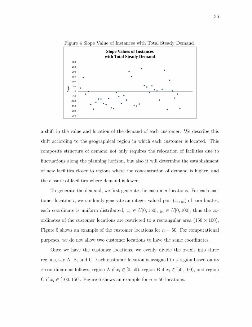
36

Figure 4 Slope Value of Instances with Total Steady Demand

Slope Values of Instances

150

200

250

300

with Total Steady Demand

100

-50

0

50

100

0 5 10 15 20 25 30 35 40 45

Slop

e

-250

-200

-150

-100

a shift in the value and location of the demand of each customer. We describe this

shift according to the geographical region in which each customer is located. This

composite structure of demand not only requires the relocation of facilities due to

fluctuations along the planning horizon, but also it will determine the establishment

of new facilities closer to regions where the concentration of demand is higher, and

the closure of facilities where demand is lower.

To generate the demand, we first generate the customer locations. For each cus-

tomer location i, we randomly generate an integer valued pair (xi, yi) of coordinates;

each coordinate is uniform distributed, xi ∈ U [0, 150], yi ∈ U [0, 100], thus the co-

ordinates of the customer locations are restricted to a rectangular area (150× 100).

Figure 5 shows an example of the customer locations for n = 50. For computational

purposes, we do not allow two customer locations to have the same coordinates.

Once we have the customer locations, we evenly divide the x-axis into three

regions, say A, B, and C. Each customer location is assigned to a region based on its

x-coordinate as follows, region A if xi ∈ [0, 50), region B if xi ∈ [50, 100), and region

C if xi ∈ [100, 150]. Figure 6 shows an example for n = 50 locations.

37

Figure 5 Customer Locations14 3833 5930 65

Customer locations5030 65

109 28137 9057 95

105 636 5291 4950

60708090

100

Axi

s

n = 50

110 92117 90117 7489 39

115 4636 1698 89

010203040

0 10 20 30 40 50 60 70 80 90 100 110 120 130 140 150

y-A

A i98 89131 479 99

x-Axis

Figure 6 Customer Locations by Region

Customer locations by region

100

xis

Customer locations by regionn = 50

0

0 50 100 150

y-A

x

Region A Region B Region C

x-Axis

The demand for each customer in each period is randomly generated from a

discrete uniform distribution depending on the region its x-coordinate belongs to.

For all demand structures, the total demand of customers in region A is decreasing

in value over the entire time horizon. In region B, the total demand increases during

the first third of the time horizon, then it remains stable up to the second third, and

finally decreases during the last third of the time horizon. Finally in region C, the

total demand is increasing along the time horizon. Figure 7 shows the total demand

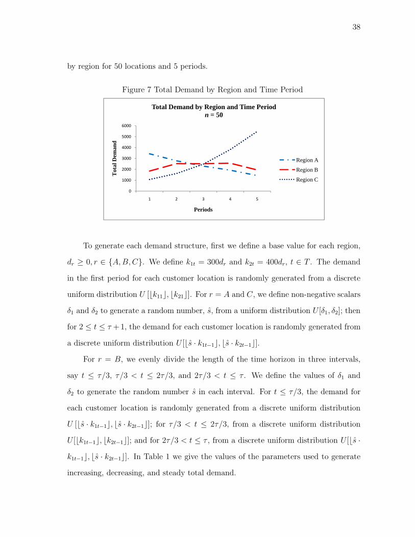
38

by region for 50 locations and 5 periods.

Figure 7 Total Demand by Region and Time Period

Total Demand by Region and Time Period

3000

4000

5000

6000

Dem

and

Total Demand by Region and Time Periodn = 50

Region A

0

1000

2000

3000

1 2 3 4 5

Tota

l D

Periods

Region A

Region B

Region C

To generate each demand structure, first we define a base value for each region,

dr ≥ 0, r ∈ {A, B, C}. We define k1t = 300dr and k2t = 400dr, t ∈ T . The demand

in the first period for each customer location is randomly generated from a discrete

uniform distribution U [�k11�, �k21�]. For r = A and C, we define non-negative scalars

δ1 and δ2 to generate a random number, s, from a uniform distribution U [δ1, δ2]; then

for 2 ≤ t ≤ τ +1, the demand for each customer location is randomly generated from

a discrete uniform distribution U [�s · k1t−1�, �s · k2t−1�].For r = B, we evenly divide the length of the time horizon in three intervals,

say t ≤ τ/3, τ/3 < t ≤ 2τ/3, and 2τ/3 < t ≤ τ . We define the values of δ1 and

δ2 to generate the random number s in each interval. For t ≤ τ/3, the demand for

each customer location is randomly generated from a discrete uniform distribution

U [�s · k1t−1�, �s · k2t−1�]; for τ/3 < t ≤ 2τ/3, from a discrete uniform distribution

U [�k1t−1�, �k2t−1�]; and for 2τ/3 < t ≤ τ , from a discrete uniform distribution U [�s ·k1t−1�, �s · k2t−1�]. In Table 1 we give the values of the parameters used to generate

increasing, decreasing, and steady total demand.

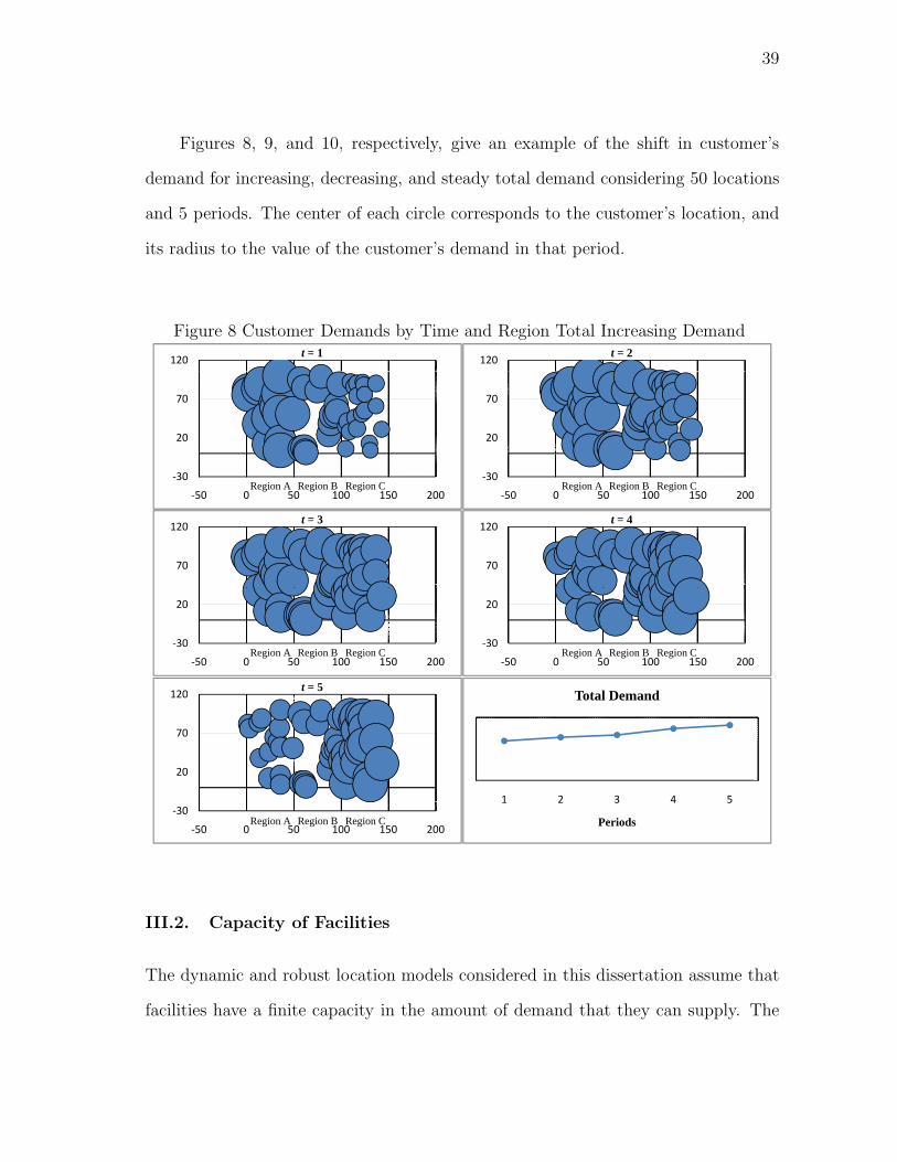
39

Figures 8, 9, and 10, respectively, give an example of the shift in customer’s

demand for increasing, decreasing, and steady total demand considering 50 locations

and 5 periods. The center of each circle corresponds to the customer’s location, and

its radius to the value of the customer’s demand in that period.

Figure 8 Customer Demands by Time and Region Total Increasing Demand

120t = 2

120t = 1

-30

20

70

-30

20

70

70

120t = 4

70

120t = 3

30

-50 0 50 100 150 200

30

-50 0 50 100 150 200Region A Region B Region C Region A Region B Region C

120t = 5

-30

20

-50 0 50 100 150 200

-30

20

-50 0 50 100 150 200

Total Demand

Region A Region B Region C Region A Region B Region C

20

70

120

1 2 3 4 5

Total Demand

-30

-50 0 50 100 150 200PeriodsRegion A Region B Region C

III.2. Capacity of Facilities

The dynamic and robust location models considered in this dissertation assume that

facilities have a finite capacity in the amount of demand that they can supply. The

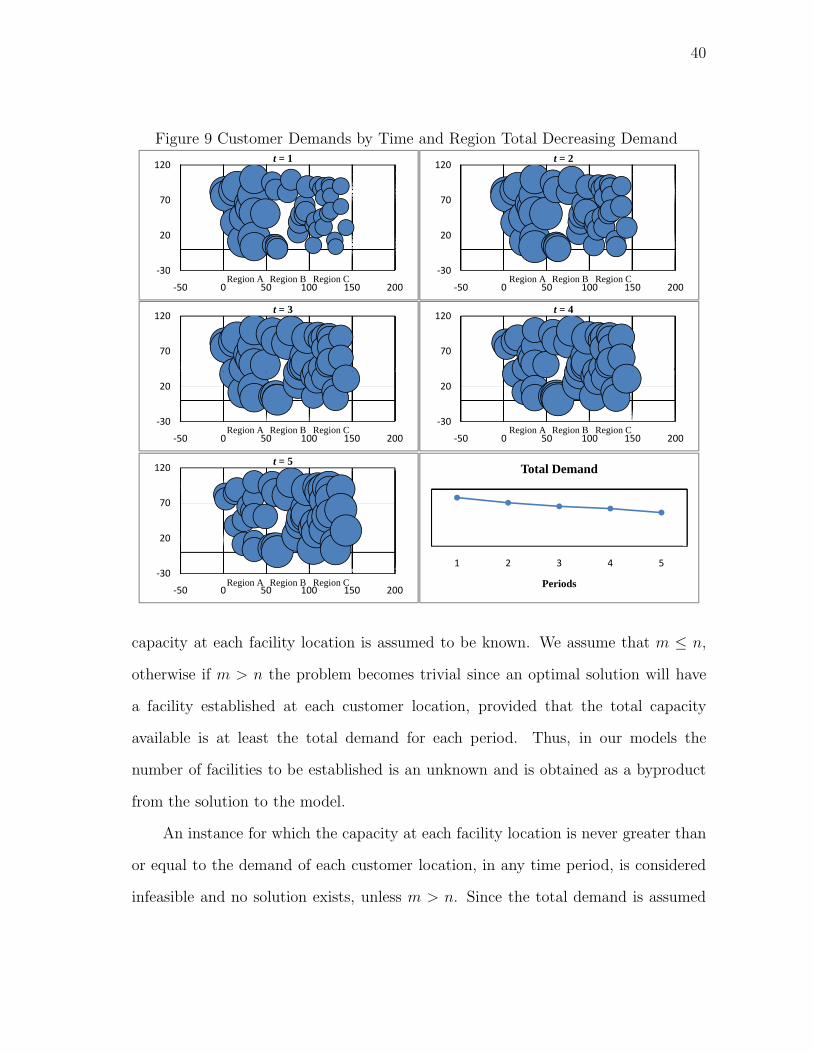
40

Figure 9 Customer Demands by Time and Region Total Decreasing Demand

120t = 2

120t = 1

-30

20

70

-30

20

70

70

120t = 4

70

120t = 3

30

-50 0 50 100 150 200

30

-50 0 50 100 150 200Region A Region B Region C Region A Region B Region C

120t = 5

-30

20

-50 0 50 100 150 200

-30

20

-50 0 50 100 150 200

Total Demand

Region A Region B Region C Region A Region B Region C

20

70

120

1 2 3 4 5

Total Demand

-30

-50 0 50 100 150 200PeriodsRegion A Region B Region C

capacity at each facility location is assumed to be known. We assume that m ≤ n,

otherwise if m > n the problem becomes trivial since an optimal solution will have

a facility established at each customer location, provided that the total capacity

available is at least the total demand for each period. Thus, in our models the

number of facilities to be established is an unknown and is obtained as a byproduct

from the solution to the model.

An instance for which the capacity at each facility location is never greater than

or equal to the demand of each customer location, in any time period, is considered

infeasible and no solution exists, unless m > n. Since the total demand is assumed

41

Figure 10 Customer Demands by Time and Region Total Steady Demand

120t = 2

120t = 1

-30

20

70

-30

20

70

70

120t = 4

70

120t = 3

30

-50 0 50 100 150 200

30

-50 0 50 100 150 200Region A Region B Region C Region A Region B Region C

120t = 5

-30

20

-50 0 50 100 150 200

-30

20

-50 0 50 100 150 200

Total Demand

Region A Region B Region C Region A Region B Region C

20

70

120

1 2 3 4 5

Total Demand

-30

-50 0 50 100 150 200PeriodsRegion A Region B Region C

to be time varying, possibly following an increasing, decreasing or steady pattern,

we would like to consider the largest possible value of the total demand over the

time horizon. The time period with the largest total demand will determine the

appropriate amount of capacity for the facilities to ensure feasibility.

We randomly generate the capacity for each facility location considering an ex-

pected number of open facilities. We also assume that the capacity at each facility

location does not change by time.

Let p be a scalar, 0 < p < 1, denoting the percentage of expected open facilities

from the total number of possible locations m. Let D = maxt∈T Dt. The base capacity

42

value, Q, for each facility location is determined by the quotient:

Q =

⌊D

pm

⌋(3.1)

Once we obtain the base capacity value Q, we randomly generate the capacity qj , j ∈J , for each facility location from a uniform distribution U [0.8Q, 1.2Q], truncating the

value towards zero.

III.3. Cost Parameters

The location models studied in this dissertation consider that cost parameters are

known or can be accurately predicted for each period of the time horizon. Making

a decision of whether to open a new facility (or close an existing facility) now or in

a future period requires the consideration of the time value of money. Usually, the

analysis of a series of future costs or investments considers the present value of these

costs. We assume that all cost parameters are computed in terms of their present

value.

We consider that shipments of demand from facilities to customers incur a trans-

portation cost proportional to quantity and distance. Let α > 0 denote the per unit

distance per unit demand cost. The distance, dij, between locations i ∈ I and j ∈ J

is computed using the Euclidean or straight-line metric:

dij =[(xi − xj)

2 + (yi − yj)2] 1

2 , i ∈ I, j ∈ J (3.2)

The transportation cost, cijt, for shipping demand of customer location i from a

facility at location j in period t is computed as follows:

cijt = αwitdij, i ∈ I, j ∈ J, t ∈ T (3.3)

43

For all the experiments we set α = 1, and truncated the value towards zero to obtain

integer values.

The fixed operation cost is randomly generated from a discrete uniform distri-

bution U [�, υ], 0 < � < υ. Let θ = (� + υ)/2. The fixed opening cost is randomly

generated from a uniform distribution U [0.75θ, 0.85θ], and the fixed closing cost from

a uniform distribution U [0.10θ, 0.15θ], truncating the value of each fixed cost towards

zero to obtain integer values.

The solution algorithms developed to solve our dynamic and robust location

models were coded in standard C++ code using ILOG CPLEX 9.0 and ILOG Concert

Technology (trademarks of ILOG, Inc.). All the experiments were performed on a

Dell OptiPlex 755 desktop computer with 3.16 GHz Dual Core 2 processor and 4.0

GB of memory.

III.4. Summary

In this chapter we described the time varying behavior and structure of the total

demand. We consider three total demand structures, increasing, decreasing, and

steady. We also consider a shift in the value and location of the demand for each

customer. Each customer location is assigned to a region according to its x-coordinate.

Each region defines a particular type of shifting in the value of the customer’s demand.

We also described the methods to generate the capacity of facility locations to ensure

feasible solutions for all instances, the computation of the variable transportation

cost, and the fixed costs for opening, operating, and closing facilities.

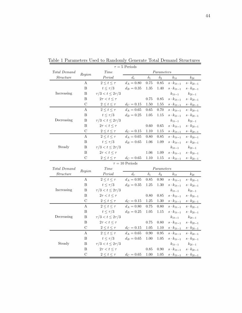
44

Table 1 Parameters Used to Randomly Generate Total Demand Structures

τ = 5 PeriodsTotal Demand

RegionTime Parameters

Structure Period dr δ1 δ2 k1t k2t

Increasing

A 2 ≤ t ≤ τ dA = 0.80 0.75 0.85 s · k1t−1 s · k2t−1

B t ≤ τ/3 dB = 0.35 1.35 1.40 s · k1t−1 s · k2t−1

B τ/3 < t ≤ 2τ/3 k1t−1 k2t−1

B 2τ < t ≤ τ 0.75 0.85 s · k1t−1 s · k2t−1

C 2 ≤ t ≤ τ dC = 0.15 1.50 1.55 s · k1t−1 s · k2t−1

Decreasing

A 2 ≤ t ≤ τ dA = 0.65 0.65 0.70 s · k1t−1 s · k2t−1

B t ≤ τ/3 dB = 0.25 1.05 1.15 s · k1t−1 s · k2t−1

B τ/3 < t ≤ 2τ/3 k1t−1 k2t−1

B 2τ < t ≤ τ 0.60 0.65 s · k1t−1 s · k2t−1

C 2 ≤ t ≤ τ dC = 0.15 1.10 1.15 s · k1t−1 s · k2t−1

Steady

A 2 ≤ t ≤ τ dA = 0.65 0.80 0.85 s · k1t−1 s · k2t−1

B t ≤ τ/3 dB = 0.65 1.06 1.09 s · k1t−1 s · k2t−1

B τ/3 < t ≤ 2τ/3 k1t−1 k2t−1

B 2τ < t ≤ τ 1.06 1.09 s · k1t−1 s · k2t−1

C 2 ≤ t ≤ τ dC = 0.65 1.10 1.15 s · k1t−1 s · k2t−1

τ = 10 PeriodsTotal Demand

RegionTime Parameters

Structure Period dr δ1 δ2 k1t k2t

Increasing

A 2 ≤ t ≤ τ dA = 0.95 0.85 0.90 s · k1t−1 s · k2t−1

B t ≤ τ/3 dB = 0.35 1.25 1.30 s · k1t−1 s · k2t−1

B τ/3 < t ≤ 2τ/3 k1t−1 k2t−1

B 2τ < t ≤ τ 0.80 0.85 s · k1t−1 s · k2t−1

C 2 ≤ t ≤ τ dC = 0.15 1.25 1.30 s · k1t−1 s · k2t−1

Decreasing

A 2 ≤ t ≤ τ dA = 0.80 0.75 0.80 s · k1t−1 s · k2t−1

B t ≤ τ/3 dB = 0.25 1.05 1.15 s · k1t−1 s · k2t−1

B τ/3 < t ≤ 2τ/3 k1t−1 k2t−1

B 2τ < t ≤ τ 0.75 0.80 s · k1t−1 s · k2t−1

C 2 ≤ t ≤ τ dC = 0.15 1.05 1.10 s · k1t−1 s · k2t−1

Steady

A 2 ≤ t ≤ τ dA = 0.65 0.90 0.95 s · k1t−1 s · k2t−1

B t ≤ τ/3 dB = 0.65 1.00 1.05 s · k1t−1 s · k2t−1

B τ/3 < t ≤ 2τ/3 k1t−1 k2t−1

B 2τ < t ≤ τ 0.85 0.90 s · k1t−1 s · k2t−1

C 2 ≤ t ≤ τ dC = 0.65 1.00 1.05 s · k1t−1 s · k2t−1

45

CHAPTER IV

DYNAMIC CAPACITATED FIXED CHARGE LOCATION PROBLEM (DCFLP)

In this chapter, we investigate the problem of finding the locations of facilities with

limited capacity to satisfy the demand of customers over a discrete and finite time

horizon. The total demand of customers is assumed to be changing by time in a

known way, and can be split or served by one or more facilities. There are fixed costs

associated with establishing or opening new facilities, operating the facilities, and for

closing existing facilities. Also, there is a variable transportation cost for serving the

customers’ demand. The main objective is to find an optimal sequence for locating

facilities to satisfy a time varying demand while observing the capacity restrictions

over the time horizon.

The chapter is organized as follows. In Section IV.1, we give the problem state-

ment. In Section IV.2, we present the mixed integer programming formulation and

notation for the DCFLP. In Section IV.3, we develop a Lagrangian relaxation and

Benders’ decomposition algorithms to solve the DCFLP. In Section IV.4, we present

an empirical analysis using different total demand patterns to test the performance

of the solution algorithms. Finally, in Section IV.5, we summarize the results and

give concluding remarks.

IV.1. Problem Statement

Specifically, the DCFLP can be stated as follows. Consider a given group of cus-

tomers on a geographical region. Each customer has a given demand for a certain

product. Along a discrete and finite time horizon, the total demand of the customers

is changing in a known way. This situation can be related to changes in population,

46

changes in the shopping habits of customers, new trends or fashions that increase the

total demand for new products or decrease the total demand for obsolete products.

An increase or decrease of the total demand for services and goods, in a particular

geographical region, may soon require the construction of facilities or services such

as power substations, convenience stores, hospitals, schools, fire stations, etc.

The establishment of facilities is required to supply the customers’ demand over

the entire time horizon. Each facility location has a known limit or capacity in

the amount of demand that can be supplied. Each customer can be served from

one or more facilities. The shipments of demand between facilities and customers

incur a variable transportation cost proportional to quantity and distance. Further,

the establishment of a new facility incurs a fixed opening cost, which can represent

the initial investment for construction, equipment, and resources needed to start

operations. An additional fixed operating cost is incurred in each period the facility

remains operational, this can be thought of as the per period cost associated with the

initial investment or the total expenses for services and labor. Finally, if the facility

is not needed in any given period it can be closed incurring a fixed closing cost, which

represents the expenses for shutting down production or decreasing the labor force.

Establishment and closure of facilities are immediate and take place at the beginning

of each period.

The main decisions are determining the number of facilities required to supply

the demand in each period, selecting the locations to establish the facilities, and

allocating demand to facilities in such a way that the total fixed and variable costs

are minimum without exceeding the capacity of facilities over the entire time horizon.

47

IV.2. Model and Notation

In this section, we provide a mixed integer programming formulation of the DCFLP.

We use the following notation.

Parameters

I set of customer locations, i = 1, . . . , n

J set of facility locations, j = 1, . . . , m

T set of periods, t = 1, . . . , τ

fjt fixed cost for having a facility open (operating) in location j during

period t

ajt fixed cost for opening a new facility (not existing in the previous pe-

riod) in location j at the beginning of period t

bjt fixed cost for closing an existing facility (already open in the previous

period) in location j at the beginning of period t

wit demand of customer in location i during period t

qj capacity available if a facility is opened at location j

dij distance between facility at location j to customer i

α per unit distance per unit demand cost

cijt transportation cost for shipping demand of customer location i from

facility at location j in period t, cijt = αwitdij

48

Decision Variables

xijt fraction of demand of customer location i shipped from facility at

location j in period t

yjt 1 if a facility is open in location j at the beginning of period t, 0

otherwise

ujt 1 if a new facility is opened in location j at the beginning of period t,

0 otherwise

vjt 1 if an existing facility is closed in location j at the beginning of period

t, 0 otherwise

(DCFLP) min∑i∈I

∑j∈J

∑t∈T

cijtxijt +∑j∈J

∑t∈T

(fjtyjt + ajtujt + bjtvjt) (4.1)

subject to∑j∈J

xijt = 1 i ∈ I, t ∈ T (4.2)

xijt ≤ yjt i ∈ I, j ∈ J, t ∈ T (4.3)

∑i∈I

witxijt ≤ qjyjt j ∈ J, t ∈ T (4.4)

vjt − ujt + yjt − yjt−1 = 0 j ∈ J, t ∈ T (4.5)

xijt ≥ 0, yjt, ujt, vjt ∈ {0, 1} i ∈ I, j ∈ J, t ∈ T (4.6)

The objective function (4.1) includes the total cost over the time horizon; it has

two main components. The first component represents the total transportation cost

between facilities and customer locations. The second component represents the total

fixed cost for operating open facilities, opening new facilities, and closing existing

49

facilities. The constraints (4.2) are the demand constraints (for each customer, all

the demand must be met), (4.3) ensure that demand is allocated to open facilities,

(4.4) are the capacity constraints (no facility can supply more than its capacity), (4.5)

are the logic constraints for relocation, and (4.6) are the nonnegativity and integrality

constraints.

Note that decision variables xijt being continuous allows the demand of each

customer location to be split between open facilities, this is called multi-sourcing.

If these decision variables are restricted to be binary integers, then the demand of

each customer must be served by only one of the open facilities, this is called single-

sourcing.

The logic constraints (4.5) state that a facility can be opened (closed) only if it

was closed (opened) in the previous period. If there are not existing facilities at the

beginning of the time horizon, then we can set yj0 = 0, ∀j ∈ J . This set of constraints

also helps to incorporate the fixed costs for opening and closing the facilities. Table 2

shows the values of the binary integer decision variables for all possible combinations.

Table 2 Possible Values for Location Decision Variables

yjt−1 yjt ujt vjt Implies

0 0 0 0 No facility in location j

1 0 0 1 Existing facility is closed

1 1 0 0 Facility remains open

0 1 1 0 New facility is opened

An optimal solution to the DCFLP model returns the values of the decision

variables indicating for each time period the location of open facilities, the amount

of demand from each customer allocated to each open facility, and the period and

location where facilities are to be opened or closed.

50

The Capacitated Fixed Charge Location Problem (CFLP) is known to be NP-

hard (Cornuejols et al., 1991). The DCFLP, which has the additional dimension of

time in the number of decision variables and constraints, is also NP-hard since it

contains the CFLP as a special case. For practical size problems, solution methods

developed for mixed integer programs may be inefficient in trying to solve the entire

model at once (such as branch and bound). In the next section we develop two

efficient solution algorithms for the DCFLP that exploit the special structure of the

model.

IV.3. Solution Procedure

In this section, we develop a Lagrangian relaxation and Benders’ decomposition al-

gorithms to solve the DCFLP.

IV.3.1. Lagrangian Relaxation

The Lagrangian relaxation approach considers the relaxation of a set of constraints by

incorporating it into the objective function using a set of Lagrange multipliers. The

set of Lagrange multipliers is a penalty imposed to solutions that violate the relaxed

set of constraints. The purpose of this type of relaxation is to obtain a Lagrangian

problem which is easier to solve than the original problem. The Lagrangian relax-

ation approach was introduced by Held and Karp (1970, 1971) to solve the traveling

salesman problem.

Lagrangian relaxation is considered to be an efficient solution method for the

CFLP. Applications of the Lagrangian relaxation for the CFLP consider the relax-

ation of different sets of constraints. Results and analysis of different implementa-

tions to solve the CFLP can be found in Geoffrion (1974), Geoffrion and McBride

51

(1978), Nauss (1978), Christofides and Beasley (1983), Nemhauser and Wolsey (1988),

Beasley (1988), Beasley (1993), and Baker and Sheasby (1999) for the multi-source

case; Barcelo and Casanovas (1984), Klincewicz and Luss (1986), Sridharan (1993),

Holmberg et al. (1999), and Hindi and Pienkosz (1999) for the single-source case.

Consider relaxing constraints (4.4) and incorporating them into the objective

function with associated non-negative Lagrange multipliers λjt. We obtain the fol-

lowing Lagrangian subproblem after rearranging terms:

LR(λ) = minx,y

∑i∈I

∑j∈J

∑t∈T

(cijt + witλjt)xijt +∑j∈J

∑t∈T

(fjt − qjλjt) yjt (4.7)

+∑j∈J

∑t∈T

(ajtujt + bjtvjt)

subject to∑j∈J

xijt = 1 i ∈ I, t ∈ T (4.8)

xijt ≤ yjt i ∈ I, j ∈ J, t ∈ T (4.9)

∑i∈I

wit ≤∑j∈J

qjyjt t ∈ T (4.10)

vjt − ujt + yjt − yjt−1 = 0 j ∈ J, t ∈ T (4.11)

xijt ≥ 0, yjt, ujt, vjt ∈ {0, 1} i ∈ I, j ∈ J, t ∈ T (4.12)

Here we have added the surrogate constraints (4.10) to the relaxed problem. This

set of surrogate constraints follows from constraint set (4.2) and (4.3), summing over

j ∈ J . These constraints are useful in obtaining feasible solutions since we get a set

of open facilities with enough capacity to satisfy the demand in each period. This

particular type of relaxation has been proven to give a stronger bound over other

52

possible relaxations for the CFLP (Cornuejols et al., 1977).

Note that we have added a non-positive term into the objective function, thus

LR(λ) = Z is a lower bound for the objective function value, Z, of the DCFLP. For

given values of the decision variables, yjt, ujt, and vjt an upper bound can be obtained

by solving the following transportation problem:

TP (x|y) = min∑i∈I

∑j∈J

∑t∈T

cijtxijt +∑j∈J

∑t∈T

(fjtyjt + ajtujt + bjtvjt) (4.13)

subject to∑j∈J

xijt = 1 i ∈ I, t ∈ T (4.14)

∑i∈I

witxijt ≤ qj yjt j ∈ J, t ∈ T (4.15)

xijt ≥ 0 i ∈ I, j ∈ J, t ∈ T (4.16)

Problem TP (x|y) separates into |T | independent transportation problems (one for

each period t ∈ T ). The objective function value, TP (x|y) = Z, is an upper bound

for the objective function value, Z∗, of any optimal solution to the DCFLP, i.e.,

LR(λ) = Z ≤ Z∗ ≤ Z = TP (x|y).

Thus, an optimal solution can be obtained by closing the optimality gap between

the lower and upper bound. Since the inequality LR(λ) ≤ Z holds for all λ, we need

to find a vector λ of Lagrange multipliers that gives the largest lower bound. In other

words, we need to solve the Lagrangian dual:

ZLD(λ) = maxλ

LR(λ) (4.17)

The function ZLD(λ) is a piece-wise linear concave function of λ, non-differentiable

53

at the maximum point (Fisher, 2004). The maximum point can be obtained using

the subgradient optimization procedure (Held et al., 1974).

At each iteration of the subgradient procedure, a set of Lagrange multipliers is

given as input to the Lagrangian subproblem LR(λ). A new feasible solution and

upper bound are obtained solving TP (x|y). The values of the Lagrange multipliers

are updated and the process is repeated.

Since the convergence of the subgradient procedure is not guaranteed, we need

to keep track of the values of the best lower and upper bound. We can stop the

subgradient method when the difference between the best upper and lower bound are

within a predefined threshold or after a given number of iterations.

At each iteration k in the subgradient method, the value of the step size, πk, is

updated as follows:

πk =δk(ZUB − Zk

lb

)∑j∈J

∑t∈T

(∑i∈I

witxkijt − qjy

kjt

)2 (4.18)

where ZUB is the best upper bound, Zklb the optimal objective function value of

Lagrangian subproblem for given Lagrange multipliers λkjt, δk a scalar, 0 < δk ≤ 2,

xkijt and yk

jt the optimal decision variables for Lagrangian subproblem.

For ZLD(λ) to give a lower bound, it is necessary that at each iteration k of the

subgradient optimization procedure we adjust the value of the non-negative Lagrange

multipliers λjt as follows:

λk+1jt = max

{0, λk

jt + πk

(∑i∈I

witxkijt − qjy

kjt

)}j ∈ J, t ∈ T (4.19)

Observe that violations to constraints (4.4) are penalized by increasing the value of

the associated Lagrange multipliers; thus the Lagrangian subproblem will try to find

54

solutions with the least level of violation to the capacity constraints.

Display 1 presents the pseudo-code of the subgradient optimization algorithm to

solve the DCFLP. We define the following notation used in the pseudo-code of the

solution algorithms:

ε non-negative threshold, 0 ≤ ε < 1

ε positive scalar, 0 < ε < 1

β positive scalar, 0 < β < 1

∞ a very large number

S best feasible solution

Zklb trial lower bound

ZLB best lower bound

Zkub trial upper bound

ZUB best upper bound

M maximum number of iterations

N predefined number of iterations without improvement in the lower

bound value

55

Display 1 Pseudo-code subgradient optimization algorithm

1: Initialize k ← 0, �← 0, ZLB ← −∞, ZUB ←∞, δk, λkjt

2: while k ≤ M do

3: Solve LR(λ)

4: Zklb ← LR(λ)

5: if Zklb > ZLB then

6: ZLB ← Zklb

7: �← 0

8: else

9: �← �+ 1

10: if � = N then

11: δk ← βδk

12: end if

13: end if

14: Solve TP (x|y)15: Zk

ub ← TP (x|y)16: if Zk

ub < ZUB then

17: ZUB ← Zkub

18: Record S

19: end if

20: if (ZUB − ZLB) /ZUB ≤ ε or δk ≤ ε then

21: Stop

22: else

23: Update πk, λk+1jt

24: end if

25: k ← k + 1

26: end while

27: Return S,ZUB

The optimality gap between the best lower and upper bound, (ZUB − ZLB) /ZUB, is

computed in the same way CPLEX computes the optimality gap. The initial values

of the Lagrange multipliers, λ0jt, can be set to zero or to a predefined value. The

positive scalar β is used to decrease the value of δk, when the best lower bound fails

to improve after N consecutive iterations of the subgradient optimization procedure.

When the value of the best upper bound is updated, we record the current feasible

solution S (set of open facilities and allocation of customers to facilities), which at

56

termination is returned as the best feasible solution together with the best upper

bound value.

The main advantage of using Lagrangian relaxation to solve the DCFLP is in

the problem structure. By relaxing the capacity constraints (4.4) we obtain a La-

grangian subproblem that is at most as difficult to solve as a dynamic Uncapacitated

Facility Location Problem (UFLP), which does not have the integrality property.

Furthermore, to obtain a feasible solution and upper bound, we solve a multi-period

transportation problem (linear program), which can be efficiently solved. In Section

IV.4, we conduct an empirical analysis to test the performance of the Lagrangian

relaxation algorithm in solving the DCFLP.

IV.3.2. Benders’ Decomposition

The DCFLP model has a special structure. For fixed values of the location variables

the resulting problem is a multi-period transportation problem (a linear program).

Thus, we can decompose the problem into two subproblems, one which with the

binary integer variables gives a solution with a set of open facilities, and a problem

with continuous variables that allocates the demand of customers to facilities. This

special structure can be exploited using Benders’ decomposition (Benders, 1962).

The main idea behind Benders’ decomposition is to separate or decompose a lin-

ear mixed integer program into two smaller problems (or subproblems) by separating

the continuous variables from the integer variables. One subproblem is constructed

with only continuous variables, called the Benders’ subproblem. The integer variables,

or complicating variables, are part of the second subproblem called the Benders’ mas-

ter problem which has only one additional continuous variable.

Applications of Benders’ decomposition to solve the CFLP can be found in Ge-

offrion and Graves (1974) for the multi-commodity distribution system design (a

57

generalization of the CFLP), McDaniel and Devine (1977) for the linear program-

ming relaxation approach to solve the master problem during early iterations of the

decomposition algorithm, Van Roy (1986) for the cross decomposition approach that

combines Lagrangian relaxation and Benders’ decomposition, and Wentges (1996)

in the development of efficient algorithms to accelerate the convergence of Benders’

decomposition.

Depending on the structure of the problem, an optimal solution to the original

problem is obtained by successively and iteratively solving each subproblem. The

solution to the master problem is given as an input to the subproblem, which returns

a dual constraint or cut to the master problem restricting its feasible region. The

process is repeated until the optimality gap between the subproblems is closed.

The special primal structure of the DCFLP makes it a good candidate for Ben-

ders’ decomposition. For given values of the location variables, yjt, we obtain the

following Benders’ subproblem (a transportation problem):

(SPy) min∑i∈I

∑j∈J

∑t∈T

cijtxijt (4.20)

subject to∑j∈J

xijt = 1 i ∈ I, t ∈ T (4.21)

xijt ≤ yjt i ∈ I, j ∈ J, t ∈ T (4.22)

∑i∈I

witxijt ≤ qj yjt j ∈ J, t ∈ T (4.23)

xijt ≥ 0 i ∈ I, j ∈ J, t ∈ T (4.24)

58

The associated dual of the subproblem:

(DSPy) max∑i∈I

∑t∈T

λit −∑i∈I

∑j∈J

∑t∈T

yjtμijt −∑j∈J

∑t∈T

qj yjtγjt (4.25)

subject to

λit − μijt − witγjt ≤ cijt i ∈ I, j ∈ J, t ∈ T (4.26)

λit unrestricted, μijt ≥ 0, γjt ≥ 0 i ∈ I, j ∈ J, t ∈ T (4.27)

which can be further decomposed into |T | independent dual subproblems (one for

each period t ∈ T ). Since the feasible region of the primal subproblem is non-empty

and bounded, we do not need to consider the extreme rays of the feasible region of

the dual subproblem.

Let{(λk, μk, γk) : k ∈ P

}denote all the extreme points of (DSPy). Let ρk denote

the objective function value corresponding to the kth extreme point, that is:

ρk =∑i∈I

∑t∈T

λkit −

∑i∈I

∑j∈J

∑t∈T

yjtμkijt −

∑j∈J

∑t∈T

qj yjtγkjt, k ∈ K ⊆ P (4.28)

where K is an appropriate index set. Since at least one optimal solution for a linear

program occurs at an extreme point of its feasible region, the optimal solution to

the dual subproblem, ρ∗, is at least as large as any objective function value ρk for

all extreme points k ∈ P (since this is a maximization problem). Thus, we have the

following Benders’ master problem:

59

(MPK) min ρ +∑j∈J

∑t∈T

(fjtyjt + ajtujt + bjtvjt) (4.29)

subject to

ρ ≥∑i∈I

∑t∈T

λkit −

∑i∈I

∑j∈J

∑t∈T

μkijtyjt −

∑j∈J

∑t∈T

qjγkjtyjt k ∈ K ⊆ P (4.30)

∑i∈I

wit ≤∑j∈J

qjyjt t ∈ T (4.31)

vjt − ujt + yjt − yjt−1 = 0 j ∈ J, t ∈ T (4.32)

ρ ≥ 0, yjt, ujt, vjt ∈ {0, 1} j ∈ J, t ∈ T (4.33)

where ρ represents the objective function value of the dual subproblem. We can

restrict ρ ≥ 0 as long as cijt ≥ 0. We have added the surrogate constraints (4.31) to

the master problem to obtain a feasible solution for (SPy).

Note that the number of extreme points of the dual subproblem may be very

large. We do not need to enumerate all the constraints (4.30) explicitly since at an

optimal solution of the master problem only a subset of constraints (4.30) is expected

to be binding. If we consider only a subset of constraints (4.30), then we will obtain

a lower bound on the optimal objective function value of the DCFLP.

An upper bound can be obtained for fixed values of the location variables, solving

the associated transportation problems and then adding the corresponding fixed cost

for operation and relocation of facilities. Each time we solve the primal and dual

subproblems we obtain another constraint of the form (4.30), thus tightening the

lower bound obtained from the master problem.

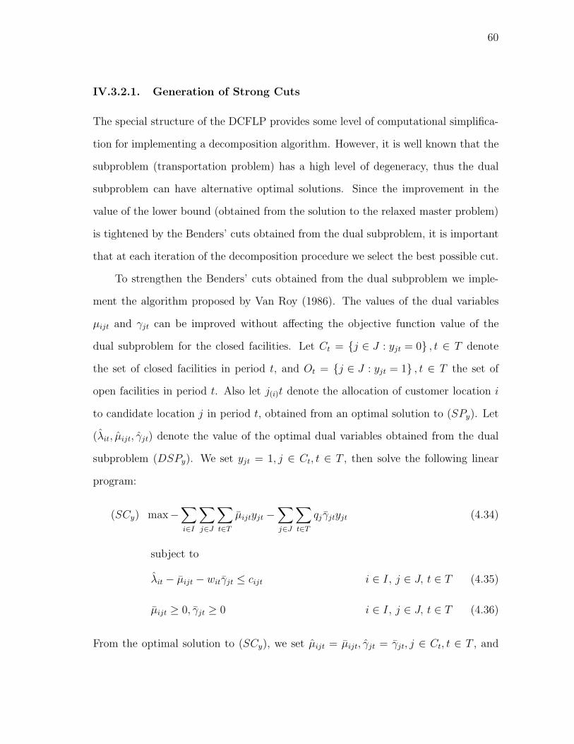
60

IV.3.2.1. Generation of Strong Cuts

The special structure of the DCFLP provides some level of computational simplifica-

tion for implementing a decomposition algorithm. However, it is well known that the

subproblem (transportation problem) has a high level of degeneracy, thus the dual

subproblem can have alternative optimal solutions. Since the improvement in the

value of the lower bound (obtained from the solution to the relaxed master problem)

is tightened by the Benders’ cuts obtained from the dual subproblem, it is important

that at each iteration of the decomposition procedure we select the best possible cut.

To strengthen the Benders’ cuts obtained from the dual subproblem we imple-

ment the algorithm proposed by Van Roy (1986). The values of the dual variables

μijt and γjt can be improved without affecting the objective function value of the

dual subproblem for the closed facilities. Let Ct = {j ∈ J : yjt = 0} , t ∈ T denote

the set of closed facilities in period t, and Ot = {j ∈ J : yjt = 1} , t ∈ T the set of

open facilities in period t. Also let j(i)t denote the allocation of customer location i

to candidate location j in period t, obtained from an optimal solution to (SPy). Let

(λit, μijt, γjt) denote the value of the optimal dual variables obtained from the dual

subproblem (DSPy). We set yjt = 1, j ∈ Ct, t ∈ T , then solve the following linear

program:

(SCy) max−∑i∈I

∑j∈J

∑t∈T

μijtyjt −∑j∈J

∑t∈T

qj γjtyjt (4.34)

subject to

λit − μijt − witγjt ≤ cijt i ∈ I, j ∈ J, t ∈ T (4.35)

μijt ≥ 0, γjt ≥ 0 i ∈ I, j ∈ J, t ∈ T (4.36)

From the optimal solution to (SCy), we set μijt = μijt, γjt = γjt, j ∈ Ct, t ∈ T , and

61

leave the previous values of the dual variables, μijt, γjt, j ∈ Ot, t ∈ T , unchanged.

Note that, constraints (4.35) guarantee that (λjt, μijt, γjt) is a feasible solution to the

dual subproblem.

IV.3.2.2. Generation of Pareto-Optimal Cuts

The generation of strong cuts produces significant savings in computation time for

the decomposition procedure. However, we can further improve the Benders’ cuts by

considering the closed and open facilities. This procedure relies on the concept of

pareto-optimal cuts introduced by Magnanti and Wong (1981). The main idea is to

generate a cut that dominates any other cut, that is, a constraint which is tighter

than any other. This is called a pareto-optimal cut.

Wentges (1996) developed an algorithm to generate pareto-optimal cuts for the

CFLP by considering the open and closed facilities. Observe that, from the relation-

ship between the primal and dual subproblems, the value of the dual variables λit

represent the cost for serving demand of customer i in period t, and the value of the

dual variables μijt the cost for allocating costumer i to facility j in period t. The fair

cost that this customer should pay for being served by facility j(i), which is closer

and more convenient, can be thought of as the additional cost that this customer

would have to pay for being served by the second nearest facility. Thus, for the open

facilities we can increase the value of λit and γjt, and decrease the cost (or give a

reward) of μij(i)t. In doing so, the objective function value of the dual subproblem

remains unchanged and constraints (4.35) are satisfied. However, the improvement

on the value of the dual variables λit could be too high since the closed facilities are

not considered. It is possible that customer i could be better served by one of the

closed facilities. Thus, in addition to the open facilities we can improve the value of

the dual variables by considering the closed facilities.

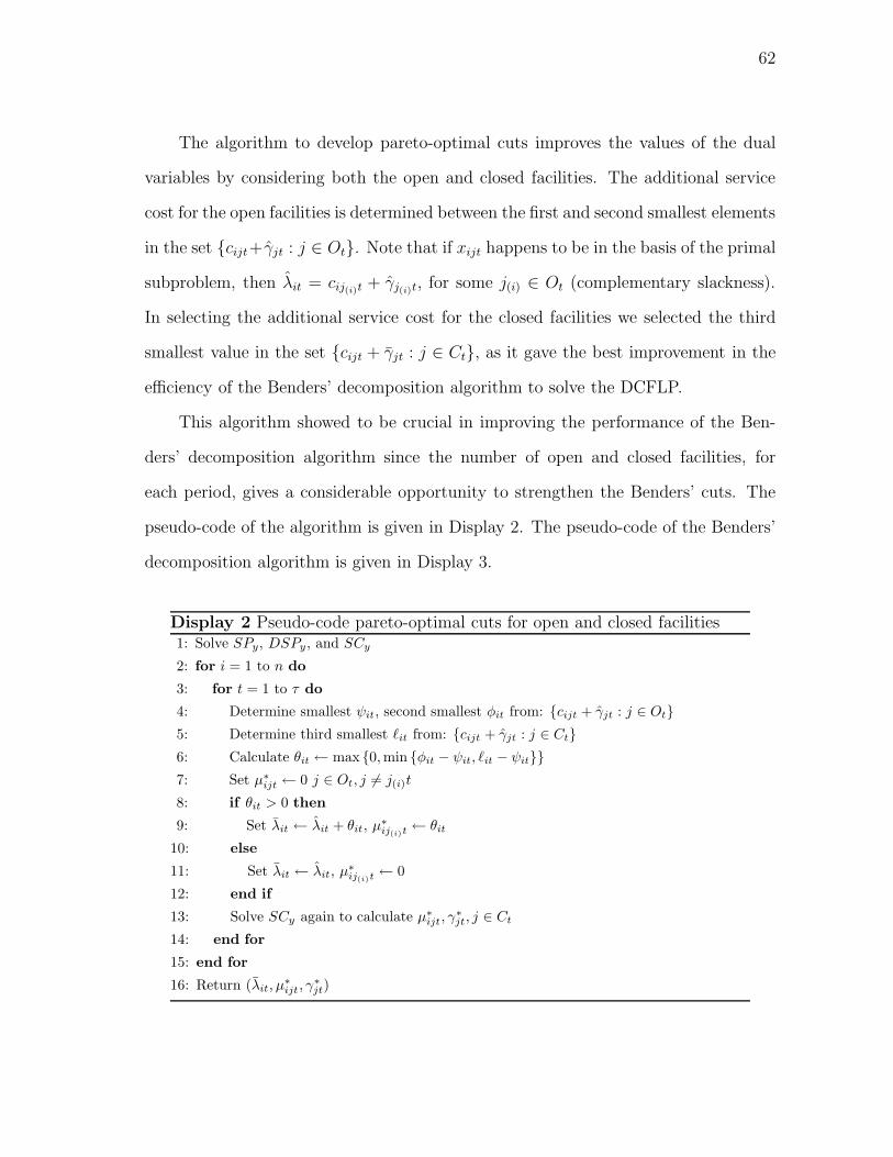
62

The algorithm to develop pareto-optimal cuts improves the values of the dual

variables by considering both the open and closed facilities. The additional service

cost for the open facilities is determined between the first and second smallest elements

in the set {cijt+γjt : j ∈ Ot}. Note that if xijt happens to be in the basis of the primal

subproblem, then λit = cij(i)t + γj(i)t, for some j(i) ∈ Ot (complementary slackness).

In selecting the additional service cost for the closed facilities we selected the third

smallest value in the set {cijt + γjt : j ∈ Ct}, as it gave the best improvement in the

efficiency of the Benders’ decomposition algorithm to solve the DCFLP.

This algorithm showed to be crucial in improving the performance of the Ben-

ders’ decomposition algorithm since the number of open and closed facilities, for

each period, gives a considerable opportunity to strengthen the Benders’ cuts. The

pseudo-code of the algorithm is given in Display 2. The pseudo-code of the Benders’

decomposition algorithm is given in Display 3.

Display 2 Pseudo-code pareto-optimal cuts for open and closed facilities1: Solve SPy, DSPy, and SCy

2: for i = 1 to n do

3: for t = 1 to τ do

4: Determine smallest ψit, second smallest φit from: {cijt + γjt : j ∈ Ot}5: Determine third smallest �it from: {cijt + γjt : j ∈ Ct}6: Calculate θit ← max {0,min {φit − ψit, �it − ψit}}7: Set μ∗

ijt ← 0 j ∈ Ot, j �= j(i)t

8: if θit > 0 then

9: Set λit ← λit + θit, μ∗ij(i)t

← θit

10: else

11: Set λit ← λit, μ∗ij(i)t

← 0

12: end if

13: Solve SCy again to calculate μ∗ijt, γ

∗jt, j ∈ Ct

14: end for

15: end for

16: Return (λit, μ∗ijt, γ

∗jt)

63

Display 3 Pseudo-code Benders’ decomposition algorithm1: Initialize k ← 0, ZLB ← −∞, ZUB ←∞2: Solve MPK

3: Zklb ←MPK

4: if Zklb > ZLB then

5: ZLB ← Zklb

6: end if

7: while k ≤ M do

8: Solve DSPy

9: Zkub ← DSPy + fixed costs

10: if Zkub < ZUB then

11: ZUB ← Zkub

12: Record S

13: end if

14: if (ZUB − ZLB)/ZUB ≤ ε then

15: Stop

16: else

17: Obtain pareto-optimal cut (λit, μ∗ijt, γ

∗jt)

18: Solve MPK with (λit, μ∗ijt, γ

∗jt)

19: Zklb ←MPK

20: if Zklb > ZLB then

21: ZLB ← Zklb

22: end if

23: if (ZUB − ZLB)/ZUB ≤ ε then

24: Stop

25: end if

26: end if

27: k ← k + 1

28: end while

29: Return S,ZUB

During the decomposition procedure, it is possible that after several iterations the

addition of Benders’ cuts to the master problem may increase its size and the com-

putational effort to solve it. Geoffrion and Graves (1974) introduced a variant to the

Benders’ decomposition approach known as feasibility seeking or ε-optimal. The idea

behind this variant is that initially, instead of solving the master problem to optimal-

64

ity, we stop whenever we find the first feasible solution within some tolerance value of

the best upper bound, ZUB − ε. Since the solution to the master problem no longer

provides a valid lower bound for the original problem, the decomposition procedure

stops whenever the master problem is unable to find a feasible solution with a value

lower than ZUB − ε.

To obtain an ε-optimal solution for the DCFLP, the following constraint is added

to the Benders’ master problem:

ρ +∑j∈J

∑t∈T

(fjtyjt + ajtujt + bjtvjt) ≤ ZUB − ε (4.37)

In Section IV.4, we conduct an empirical analysis to test the performance of Benders’

decomposition and ε-optimal algorithms.

IV.4. Numerical Results

In this section, we conduct an empirical analysis to test the performance of the

solution algorithms developed for the DCFLP. The empirical analysis was designed

considering the three total demand structures, increasing, decreasing, and steady

(described in Chapter III); two values for n = 50 and 100 locations; two values

for τ = 5 and 10 periods; three values for the percentage of expected number of

open facilities p = 0.05, 0.10, and 0.15; and three discrete uniform distributions to

randomly generate the fixed operation cost, U [100000, 150000], U [200000, 250000],

and U [300000, 350000]. Thus, the total number of different classes of problems is 108.

For each class, we randomly generated 10 instances.

For comparison purposes, we arranged the classes for each total demand structure

into 12 clusters, each cluster containing three classes. Table 3 shows the 12 clusters

of classes. For all the experiments, we assumed that yj0 = 0, j ∈ J , i.e., no existing

65

facilities at the beginning of the first period.

Table 3 DCFLP Classes of Problems Arranged in Clusters

Parameters ParametersCluster n τ p % f Cluster n τ p % f

150 5 5 U [100000, 150000]

7100 5 5 U [100000, 150000]

50 5 10 U [100000, 150000] 100 5 10 U [100000, 150000]50 5 15 U [100000, 150000] 100 5 15 U [100000, 150000]

250 5 5 U [200000, 250000]

8100 5 5 U [200000, 250000]

50 5 10 U [200000, 250000] 100 5 10 U [200000, 250000]50 5 15 U [200000, 250000] 100 5 15 U [200000, 250000]

350 5 5 U [300000, 350000]

9100 5 5 U [300000, 350000]

50 5 10 U [300000, 350000] 100 5 10 U [300000, 350000]50 5 15 U [300000, 350000] 100 5 15 U [300000, 350000]

450 10 5 U [100000, 150000]

10100 10 5 U [100000, 150000]

50 10 10 U [100000, 150000] 100 10 10 U [100000, 150000]50 10 15 U [100000, 150000] 100 10 15 U [100000, 150000]

550 10 5 U [200000, 250000]

11100 10 5 U [200000, 250000]

50 10 10 U [200000, 250000] 100 10 10 U [200000, 250000]50 10 15 U [200000, 250000] 100 10 15 U [200000, 250000]

650 10 5 U [300000, 350000]

12100 10 5 U [300000, 350000]

50 10 10 U [300000, 350000] 100 10 10 U [300000, 350000]50 10 15 U [300000, 350000] 100 10 15 U [300000, 350000]

The performance of the Lagrangian relaxation algorithm relies on the value of

the parameters used by the subgradient optimization procedure. To determine the

most appropriate values for these parameters, we solved two instances per class for

each total demand structure. For the initial value of the Lagrange multipliers, we

considered the values of 0 and 1.0; for the initial value of δ0, 2.0, 1.8, and 1.5; for β,

0.50, 0.60, and 0.80; and for N , 5, 10, and 20 iterations. We selected the combination

of parameters with the lowest average optimality gap and lowest average solution time

in seconds over all the classes. We set the initial values of the Lagrange multipliers

λ0jt = 0, j ∈ J, t ∈ T , δ0 = 1.8, M = 200, N = 5, and β = 0.5, since this combination

gave the best over all performance for each total demand structure.

At each iteration of the subgradient algorithm, we solved the Lagrangian sub-

66

problem using CPLEX with early stopping at 1.0% optimality gap. We took the

lower bound value from the solution given by CPLEX at early stopping and set it

as the trial lower bound. Note that this approach gives a valid lower bound. The

set of open facilities obtained from the Lagrangian subproblem was given as an input

to CPLEX to solve |T | transportation problems to optimality and obtain the value

of the trial upper bound. The stopping criteria for the subgradient algorithm was

set to the first occurrence of three conditions: 1.5% optimality gap, δk ≤ 0.001, and

M = 200 iterations.

For Benders’ decomposition and ε-optimal algorithms, we solved the master prob-

lem initially with a large optimality gap and gradually reduced it as the algorithm

progressed. We followed this approach since in the initial iterations the master prob-

lem does not have enough information from the dual subproblem until several Benders’

cuts are added. During the first 10 iterations of both decomposition algorithms, we

solved the master problem using CPLEX with early stopping considering an optimal-

ity gap of 5%. This optimality gap was reduced every 10 iterations to 3.5, 2.5, 1.5,

and 1.0%. To determine this sequence of values for early stopping, we solved two

instances for each class and for each total demand structure. We defined three stages

for the optimality gap of the master problem: initial, intermediate, and final. For

the initial stage, we considered 5 and 10% optimality gap; for the intermediate stage,

we considered three percentage values: 3.5, 2.5, and 1.5% for initial stage gap of 5%,

and 8.5, 4.5, and 1.5% for initial stage gap of 10%. For the final stage, we considered

a percentage gap of 1.0%. For the number of iterations, we considered 5, 10, and 15

iterations. We selected the combination that gave the lower average optimality gap

and lower average solution time over all the classes.

At each iteration of the decomposition algorithm, we solved the master problem

using CPLEX, with early stopping as described above. We took the lower bound value

67

from the solution given by CPLEX and set it as the trial lower bound. To compute

the upper bound, the set of open facilities obtained from the master problem was

given as an input to CPLEX to solve |T | dual problems to optimality. The value of

the trial upper bound at iteration k was computed by Zkub = DSPy plus the associated

fixed opening, operation, and closing costs. The primal subproblem and the strong-

cuts algorithm were also solved using CPLEX. The stopping criteria for the Benders’

decomposition algorithms was set to 1.5% optimality gap and M = 200 iterations.

The benchmark solutions were obtained solving the DCFLP model with CPLEX,

which uses a branch and cut algorithm, using default settings. We used early stopping

with an optimality gap of 1.5%, and recorded the lower and upper bound values.

For all the experiments, we limited the running time for each instance with

n = 50 to 3000 seconds, and n = 100 to 4000 seconds. For each class, we reported the

average (Avg.) and maximum (Max.) value of the optimality gap and the average

and maximum solution time. Tables 4, 5, and 6 on pages 68, 69, and 70 respectively,

describe the performance of the solution algorithms for each total demand structure.

We denote by NS the benchmark classes Not Solved by CPLEX within the maximum

solution time (in most cases, the solution to the root node exceeded the maximum

running time).

As part of the empirical analysis, we considered the analysis of the cost split, in

percentage value, of the total cost corresponding to variable transportation cost and

fixed opening, operation, and closing costs. For each class, we selected the solution

with minimum average optimality gap to compute the average percentage for each

type of cost. In Table 7 on page 71, we report the average cost split per class for each

total demand structure. The analysis of the cost split is important, we can identify

a relation between the efficiency of the solution algorithms and the structure of the

cost split for each class of problems.

68

Tab

le4

DC

FLP

Com

puta

tion

alR

esult

sIn

crea

sing

Dem

and

Bra

nch

&C

utLag

rang

ian

Rel

axat

ion

Ben

ders

’Dec

ompo

sition

ε-O

ptim

alG

ap(%

)T

ime

(sec

.)G

ap(%

)T

ime

(sec

.)G

ap(%

)T

ime

(sec

.)T

ime

(sec

.)C

lust

erA

vg.

Max

.A

vg.

Max

.A

vg.

Max

.A

vg.

Max

.A

vg.

Max

.A

vg.

Max

.A

vg.

Max

.

12.

587.

7093

0.06

3000

.18

1.13

1.48

10.0

533

.09

1.48

1.50

45.7

468

.59

9.16

22.9

13.

915.

9026

71.9

230

00.3

41.

321.

6017

2.62

586.

101.

451.

5056

.04

200.

0011

.80

31.0

03.

234.

7625

62.4

430

00.2

71.

351.

5362

5.47

2215

.69

1.31

1.50

27.9

957

.38

5.93

13.2

2

24.

2213

.70

2432

.35

3000

.31

1.20

1.49

5.62

26.2

51.

411.

4920

.61

37.4

23.

527.

275.

788.

8729

33.3

530

00.2

71.

151.

4910

.37

57.0

71.

411.

5014

.99

22.6

43.

266.

174.

066.

6729

29.4

330

00.6

31.

351.

5013

1.48

549.

101.

331.

507.

9817

.17

1.88

5.75

36.

4515

.47

2769

.05

3000

.23

0.99

1.48

15.9

511

9.83

1.39

1.49

17.2

727

.05

2.43

4.14

6.50

9.72

3000

.14

3000

.29

1.18

1.49

7.06

46.3

61.

301.

4910

.02

25.0

81.

984.

524.

356.

3730

00.1

730

00.3

31.

161.

4347

.82

446.

571.

191.

493.

8112

.00

1.24

3.33

41.

864.

2610

60.8

630

00.1

61.

121.

4923

1.29

1122

.73

2.83

5.19

2754

.52

3000

.42

2273

.30

3000

.83

5.01

7.92

3000

.36

3000

.74

1.93

3.49

1794

.73

3000

.11

2.03

3.03

2245

.70

3000

.31

1570

.16

3000

.78

3.79

4.87

3000

.13

3000

.19

2.21

3.44

2755

.58

3000

.10

1.73

2.25

2492

.25

3000

.93

1092

.41

3000

.26

55.

278.

9330

00.1

830

00.3

51.

151.

4530

5.23

1416

.47

1.41

1.75

732.

0430

00.3

317

1.51

769.

006.

8410

.39

3000

.18

3000

.33

1.52

2.24

1269

.91

3000

.10

1.35

1.49

335.

6815

27.0

461

.15

149.

645.

096.

3430

00.1

430

00.2

81.

401.

5315

58.3

330

00.1

01.

391.

4912

7.56

313.

3336

.60

74.0

3

68.

2413

.64

3000

.25

3000

.49

1.00

1.48

209.

8911

03.3

31.

431.

5018

3.76

638.

9039

.08

128.

207.

5210

.78

3000

.15

3000

.31

1.32

1.53

258.

9320

43.7

81.

421.

4964

.74

165.

7316

.26

45.2

55.

556.

8930

00.2

030

00.4

91.

421.

8064

3.77

3000

.09

1.38

1.50

30.1

378

.00

9.99

19.3

0

72.

354.

0636

42.6

640

00.4

41.

602.

1212

74.9

630

47.0

62.

394.

4231

06.2

140

00.2

821

55.1

640

00.7

42.

423.

5536

48.0

340

00.3

92.

714.

3335

42.3

640

00.2

51.

692.

3427

64.8

740

00.2

518

53.4

140

00.6

12.

493.

5935

43.1

440

00.5

22.

904.

7535

87.3

040

00.2

51.

491.

9170

1.07

3161

.74

221.

3669

7.79

85.

999.

9140

00.4

240

00.7

31.

301.

7565

0.54

3116

.78

1.47

1.97

972.

8640

00.2

128

3.62

1630

.43

3.70

4.72

3930

.49

4000

.56

1.54

1.78

1961

.96

4000

.23

1.43

1.49

121.

6418

3.33

32.7

985

.28

2.45

4.37

3310

.76

4000

.41

1.49

1.69

3048

.84

4000

.20

1.38

1.50

20.1

468

.20

9.43

22.5

0

97.

1510

.83

4000

.31

4000

.54

1.15

1.47

122.

5453

9.54

1.41

1.50

270.

7292

7.81

45.1

417

5.24

4.17

5.03

4000

.28

4000

.38

1.44

1.84

641.

6040

00.1

51.

451.

5054

.08

130.

5616

.16

25.9

12.

624.

1732

55.1

940

00.8

21.

441.

7379

8.78

4000

.17

1.17

1.46

22.4

472

.99

5.85

9.33

1011

.30

92.4

129

60.4

440

00.7

82.

354.

7732

32.8

440

00.9

46.

979.

0040

00.7

440

00.9

040

00.5

240

00.8

25.

596.

9640

00.4

040

00.8

05.

596.

9940

00.5

240

00.7

04.

035.

1340

00.5

340

00.8

840

00.3

540

00.6

53.

524.

6440

00.6

940

00.9

45.

636.

5940

00.4

040

00.4

73.

044.

1040

00.2

240

00.8

940

00.6

340

00.9

1

119.

9823

.02

4000

.87

4000

.93

2.09

4.03

3466

.38

4000

.45

3.66

5.48

4000

.80

4000

.87

3858

.22

4000

.61

23.2

391

.75

4000

.49

4000

.95

3.57

4.67

4000

.43

4000

.52

2.18

2.69

4000

.41

4000

.90

4000

.25

4000

.84

20.4

688

.27

4000

.22

4000

.49

1.73

3.89

2403

.36

4000

.20

1.69

1.98

3245

.65

4000

.90

2593

.36

4000

.64

12N

SN

SN

SN

S1.

752.

7826

23.0

540

00.4

42.

153.

3534

11.0

740

00.9

025

20.1

240

00.1

422

.42

92.2

540

00.5

140

00.8

12.

574.

1640

00.4

040

00.5

01.

511.

5827

22.5

540

00.4

013

21.2

737

15.6

7N

SN

SN

SN

S3.

014.

8638

75.2

940

00.7

61.

421.

4876

6.44

2659

.59

434.

7621

86.9

2

69

Tab

le5

DC

FLP

Com

puta

tion

alR

esult

sD

ecre

asin

gD

eman

dB

ranc

h&

Cut

Lag

rang

ian

Rel

axat

ion

Ben

ders

’Dec

ompo

sition

ε-O

ptim

alG

ap(%

)T

ime

(sec

.)G

ap(%

)T

ime

(sec

.)G

ap(%

)T

ime

(sec

.)T

ime

(sec

.)C

lust

erA

vg.

Max

.A

vg.

Max

.A

vg.

Max

.A

vg.

Max

.A

vg.

Max

.A

vg.

Max

.A

vg.

Max

.

14.

307.

7628

77.7

630

00.2

30.

731.

191.

712.

081.

251.

4923

.55

43.1

73.

887.

365.

208.

1030

00.2

330

00.5

51.

101.

4913

.77

55.1

31.

421.

5020

.92

35.3

94.

518.

664.

085.

8029

66.0

130

00.3

01.

261.

4767

.94

251.

331.

421.

5013

.65

24.0

62.

876.

20

210

.23

12.6

230

00.0

630

00.1

30.

560.

911.

482.

141.

461.

5014

.46

21.1

92.

154.

027.

8910

.88

3000

.11

3000

.27

0.89

1.47

19.1

817

8.47

1.36

1.49

10.3

123

.31

2.12

3.64

5.68

7.91

3000

.19

3000

.39

1.00

1.36

9.17

55.2

51.

391.

492.

035.

831.

262.

53

312

.65

14.9

230

00.2

230

00.5

10.

370.

681.

401.

831.

361.

5012

.17

19.0

31.

523.

178.

8011

.11

3000

.16

3000

.34

0.84

1.29

3.06

15.9

81.

381.

503.

3618

.64

1.30

2.09

6.11

8.69

3000

.18

3000

.36

0.85

1.45

8.13

72.8

31.

271.

462.

6513

.17

1.10

1.70

48.

2411

.61

3000

.15

3000

.34

1.01

1.42

48.0

932

7.79

1.48

1.50

229.

8932

9.06

40.7

864

.08

7.89

10.9

330

00.1

630

00.3

01.

361.

9474

5.26

3000

.08

1.41

1.50

171.

2367

1.96

42.2

819

6.13

6.35

8.22

3000

.15

3000

.28

1.45

2.04

1386

.82

3000

.10

1.42

1.50

86.6

921

2.28

22.1

550

.03

513

.28

18.3

130

00.1

630

00.2

80.

661.

219.

3016

.30

1.44

1.49

58.2

686

.16

8.97

16.3

110

.10

12.8

030

00.1

330

00.2

60.

981.

4917

5.36

1148

.02

1.44

1.50

37.3

112

5.72

7.50

21.5

36.

398.

1630

00.1

130

00.2

61.

131.

4253

.89

185.

661.

341.

5015

.56

37.3

14.

988.

11

615

.80

20.5

530

00.2

630

00.5

30.

420.

887.

1815

.38

1.42

1.50

34.3

855

.08

4.31

9.16

11.2

513

.13

3000

.22

3000

.81

1.06

1.49

83.7

650

5.16

1.41

1.49

12.7

234

.55

4.01

7.67

7.20

9.29

3000

.24

3000

.50

1.00

1.49

38.0

726

9.71

1.22

1.47

7.71

27.3

43.

196.

42

77.

5213

.85

4000

.51

4000

.94

1.25

2.10

395.

8830

29.9

71.

431.

5069

0.45

2741

.11

161.

6942

4.77

4.11

5.58

4000

.29

4000

.36

1.45

1.92

1531

.85

4000

.25

1.45

1.49

288.

7399

4.61

61.6

724

0.55

2.10

3.16

3612

.82

4000

.50

1.69

2.25

2041

.14

4000

.29

1.34

1.42

79.8

526

7.88

107.

7979

0.78

89.

3411

.82

4000

.22

4000

.43

0.94

1.43

83.8

757

3.92

1.42

1.49

190.

7632

4.24

32.2

458

.38

5.17

6.72

4000

.28

4000

.41

1.29

1.46

337.

7217

24.9

51.

421.

5058

.92

179.

5216

.06

29.1

12.

543.

8440

00.3

540

00.6

61.

231.

4723

1.88

1340

.98

1.29

1.49

8.30

16.6

97.

9224

.84

910

.70

13.0

340

00.3

640

00.5

30.

651.

2328

.11

49.1

91.

431.

4810

7.85

194.

5221

.17

44.4

45.

938.

0740

00.3

040

00.4

21.

121.

4196

.16

721.

891.

341.

5021

.71

78.5

98.

0410

.69

2.69

3.74

4000

.33

4000

.53

1.14

1.43

8.67

15.2

81.

191.

496.

2915

.97

6.85

18.4

4

1059

.75

94.9

540

00.4

740

00.5

81.

822.

7429

56.1

740

00.4

13.

224.

6740

00.6

840

00.9

840

00.2

940

00.5

523

.49

92.2

240

00.4

440

00.6

32.

453.

1540

00.3

940

00.5

01.

852.

4336

90.2

040

00.4

530

16.3

440

00.5

7N

SN

SN

SN

S4.

145.

2340

00.3

840

00.4

01.

522.

1612

83.1

231

65.8

514

76.9

540

00.8

5

11N

SN

SN

SN

S1.

662.

7518

15.9

640

00.7

61.

471.

8619

36.2

340

00.4

174

1.09

1884

.45

NS

NS

NS

NS

1.69

3.32

2251

.07

4000

.48

1.43

1.49

587.

5013

07.0

213

2.29

257.

42N

SN

SN

SN

S1.

693.

3623

82.1

740

00.3

91.

331.

4913

3.61

555.

8459

.23

151.

97

12N

SN

SN

SN

S1.

392.

8714

01.0

240

00.6

11.

371.

4860

5.46

1370

.67

141.

3629

2.66

NS

NS

NS

NS

1.32

2.13

1597

.51

4000

.39

1.36

1.50

223.

6057

1.92

43.5

511

6.36

NS

NS

NS

NS

1.14

1.81

615.

6640

00.2

91.

151.

4863

.03

236.

6128

.05

73.5

5

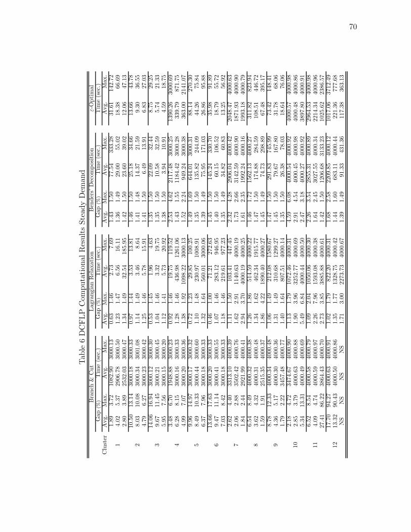
70

Tab

le6

DC

FLP

Com

puta

tion

alR

esult

sSte

ady

Dem

and

Bra

nch

&C

utLag

rang

ian

Rel

axat

ion

Ben

ders

’Dec

ompo

sition

ε-O

ptim

alG

ap(%

)T

ime

(sec

.)G

ap(%

)T

ime

(sec

.)G

ap(%

)T

ime

(sec

.)T

ime

(sec

.)C

lust

erA

vg.

Max

.A

vg.

Max

.A

vg.

Max

.A

vg.

Max

.A

vg.

Max

.A

vg.

Max

.A

vg.

Max

.

11.

893.

7210

82.9

030

00.1

30.

631.

462.

737.

691.

431.

5077

.54

333.

2831

.61

142.

724.

025.

3729

06.7

830

00.5

01.

231.

476.

5616

.11

1.36

1.49

29.0

055

.02

18.3

866

.69

2.80

3.89

2532

.03

3000

.47

1.34

1.49

32.5

418

5.95

1.42

1.50

23.6

039

.02

12.0

647

.13

210

.50

13.1

430

00.1

830

00.3

30.

971.

443.

5313

.81

1.46

1.50

25.1

834

.66

13.6

643

.78

8.03

10.0

830

00.3

430

01.0

81.

141.

493.

468.

641.

411.

4814

.37

21.5

99.

3036

.55

4.79

6.27

3000

.23

3000

.42

1.25

1.46

5.78

15.9

11.

411.

506.

4913

.91

6.83

27.0

3

314

.06

16.9

430

00.1

230

00.3

00.

531.

451.

964.

631.

351.

5022

.09

32.4

48.

7529

.25

9.67

11.4

530

00.2

130

00.4

51.

041.

463.

3219

.75

1.35

1.50

10.5

832

.59

5.74

21.3

35.

957.

5630

00.1

530

00.2

01.

121.

415.

7320

.92

1.38

1.50

3.94

10.9

14.

5918

.75

43.

486.

7019

48.8

830

00.2

30.

921.

4619

.75

119.

522.

534.

6221

17.4

830

00.2

513

90.2

630

00.6

96.

288.

1530

00.1

630

00.3

31.

281.

4643

6.98

1261

.06

1.43

1.55

1184

.42

3000

.28

339.

7987

1.75

4.99

7.07

3000

.20

3000

.36

1.38

1.92

1098

.22

3000

.13

1.52

2.24

949.

2430

00.3

836

3.00

2141

.07

59.

9614

.97

3000

.17

3000

.32

0.72

1.23

29.8

510

0.25

1.49

1.69

644.

0130

00.3

188

.14

270.

308.

4910

.33

3000

.44

3000

.60

1.10

1.48

230.

9710

08.9

11.

351.

5013

5.82

244.

0944

.26

75.8

46.

377.

9630

00.1

830

00.3

31.

321.

6456

0.01

3000

.06

1.39

1.49

75.9

517

1.03

26.8

695

.88

613

.66

17.6

330

00.2

030

00.3

30.

461.

0071

.21

272.

631.

451.

5014

5.24

330.

7035

.98

91.8

99.

4711

.14

3000

.41

3000

.55

1.07

1.46

283.

1294

6.95

1.40

1.50

60.1

510

6.52

18.7

955

.72

7.03

8.42

3000

.18

3000

.33

1.18

1.46

219.

6197

7.23

1.35

1.49

34.8

260

.83

13.2

556

.92

72.

624.

4033

13.1

040

00.3

91.

111.

5010

3.41

447.

452.

324.

2829

06.0

440

00.4

220

48.4

740

00.6

32.

062.

8835

02.4

240

00.7

61.

622.

9111

40.6

340

00.1

91.

732.

6631

42.5

940

00.9

018

71.9

340

00.9

01.

842.

4429

21.9

940

00.4

12.

943.

7040

00.1

940

00.2

51.

612.

3519

92.2

440

00.1

619

93.1

840

00.7

9

86.

548.

4940

00.3

240

00.3

81.

261.

8651

4.59

4000

.22

1.46

1.72

1562

.13

4000

.27

311.

8282

3.94

3.62

4.32

4000

.31

4000

.48

1.34

1.62

462.

3419

15.7

71.

471.

5017

4.88

284.

5910

8.51

446.

721.

591.

9125

15.3

540

00.3

71.

864.

2218

90.4

040

00.2

71.

451.

4974

.73

298.

8967

.48

395.

17

98.

7812

.33

4000

.34

4000

.48

1.06

1.49

212.

0815

80.6

71.

471.

5029

1.83

745.

9973

.42

148.

414.

365.

1740

00.3

040

00.3

61.

311.

4931

0.68

1299

.27

1.45

1.50

79.6

716

7.80

31.7

868

.06

1.79

2.22

3457

.48

4000

.77

1.40

1.64

807.

5140

00.1

41.

351.

5026

.38

78.0

318

.64

76.0

6

102.

184.

7234

74.6

740

00.9

01.

131.

7910

72.4

640

00.3

14.

596.

0840

00.5

440

00.9

240

00.5

740

00.9

82.

853.

7940

00.6

340

00.8

81.

903.

9632

52.7

740

00.6

92.

914.

5440

00.4

540

00.9

840

00.4

840

00.8

65.

3413

.31

4000

.49

4000

.69

5.49

6.84

4000

.44

4000

.50

2.47

3.18

4000

.27

4000

.92

3897

.80

4000

.91

116.

528.

5440

00.5

840

00.7

91.

092.

0410

50.0

640

00.3

02.

263.

5428

55.3

140

00.8

929

64.5

340

00.9

84.

094.

7440

00.5

940

00.9

72.

267.

9615

93.0

840

00.3

81.

642.

4530

27.5

540

00.3

422

14.3

440

00.9

627

.41

86.2

238

64.4

340

00.7

02.

733.

8538

85.8

840

00.6

11.

421.

5012

06.6

831

33.2

310

25.6

223

86.5

7

1217

.70

94.2

740

00.6

340

00.9

11.

021.

7982

2.20

4000

.31

1.68

2.58

2209

.85

4000

.12

1017

.06

3712

.49

13.3

290

.43

4000

.50

4000

.86

1.35

1.77

1328

.75

4000

.42

1.44

1.60

683.

1140

00.4

422

1.36

777.

68N

SN

SN

SN

S1.

713.

0022

73.7

340

00.6

71.

391.

4991

.33

431.

3611

7.38

363.

13

71

Tab

le7

Ave

rage

Cos

tSplit

Incr

easing

Tot

alD

eman

dD

ecre

asin

gTot

alD

eman

dSt

eady

Tot

alD

eman

dCos

tSp

lit(%

)Cos

tSp

lit(%

)Cos

tSp

lit(%

)C

lust

erTra

n.O

per.

Ope

n.C

los.

Tra

n.O

per.

Ope

n.C

los.

Tra

n.O

per.

Ope

n.C

los.

149

.13

43.3

77.

500.

0029

.70

56.2

013

.44

0.65

56.4

737

.24

6.29

0.00

23.1

863

.79

12.9

90.

0315

.35

68.3

015

.34

1.01

24.4

164

.26

11.2

80.

0416

.34

79.1

44.

520.

009.

9873

.04

16.0

10.

9716

.46

71.0

012

.50

0.03

228

.50

59.0

412

.46

0.00

18.4

766

.07

14.7

50.

7241

.33

50.3

58.

320.

0014

.20

71.7

214

.04

0.05

9.04

74.2

715

.76

0.93

15.0

072

.80

12.1

60.

049.

8385

.54

4.63

0.00

5.68

77.2

416

.10

0.98

9.83

77.2

412

.90

0.03

321

.40

64.5

913

.94

0.07

13.3

970

.53

15.3

30.

7521

.12

67.5

011

.25

0.12

10.3

075

.16

14.5

00.

046.

5976

.46

15.9

61.

0010

.91

76.5

212

.52

0.04

6.82

78.2

514

.87

0.06

4.14

78.8

616

.07

0.93

6.97

79.8

913

.11

0.03

454

.77

40.4

44.

650.

1435

.23

57.0

57.

200.

5258

.89

37.7

83.

320.

0030

.50

62.2

27.

190.

0819

.20

71.4

78.

680.

6426

.57

67.1

06.

170.

1620

.31

71.2

08.

330.

1512

.57

77.5

39.

200.

7017

.51

75.4

56.

860.

18

537

.12

55.7

57.

000.

1322

.93

68.1

88.

280.

6133

.20

60.7

95.

710.

3018

.78

73.0

78.

030.

1211

.55

78.6

79.

070.

7217

.16

75.8

66.

760.

2212

.64

81.0

36.

330.

007.

4082

.55

9.33

0.71

11.1

181

.53

7.15

0.21

629

.82

62.7

77.

340.

0817

.28

73.1

88.

860.

6825

.65

67.6

86.

330.

3314

.67

77.0

38.

240.

068.

8481

.19

9.26

0.71

12.5

580

.15

7.09

0.21

9.00

83.6

77.

330.

005.

3084

.54

9.41

0.75

8.13

84.3

07.

340.

23

736

.31

52.4

011

.17

0.13

26.0

259

.87

13.3

10.

7940

.22

50.8

68.

920.

0019

.63

66.2

713

.95

0.15

12.7

271

.13

15.3

00.

8522

.45

65.9

411

.59

0.02

12.9

372

.49

14.5

10.

078.

1774

.91

16.0

00.

9114

.46

72.5

112

.97

0.06

824

.43

63.4

012

.17

0.00

16.0

768

.61

14.4

60.

8526

.80

62.6

410

.56

0.00

12.4

673

.78

13.7

60.

007.

4476

.09

15.5

50.

9213

.54

74.0

212

.42

0.02

8.30

77.5

814

.13

0.00

4.75

78.4

215

.92

0.91

8.95

78.0

213

.02

0.02

918

.11

68.9

212

.97

0.00

11.6

272

.56

14.9

30.

9020

.31

68.2

811

.38

0.03

9.05

77.0

313

.92

0.00

5.57

77.9

215

.58

0.93

9.86

77.3

412

.78

0.02

5.93

79.7

814

.29

0.00

3.36

79.7

915

.92

0.93

6.49

80.3

013

.19

0.02

1046

.82

47.8

35.

320.

0331

.72

60.5

47.

210.

5243

.18

52.1

94.

620.

0125

.53

66.1

88.

100.

1916

.23

74.2

58.

870.

6623

.56

69.7

56.

600.

0916

.61

74.1

09.

110.

1810

.10

79.5

69.

580.

7615

.31

77.2

87.

310.

10

1133

.31

59.9

86.

660.

0520

.97

70.4

28.

020.

6029

.34

65.0

85.

550.

0316

.49

75.0

38.

340.

149.

7180

.63

9.01

0.65

14.4

078

.82

6.74

0.05

10.7

480

.56

8.61

0.10

6.19

83.8

49.

280.

689.

3483

.51

7.11

0.05

1226

.22

66.6

67.

100.

0315

.43

75.4

28.

530.

6222

.29

71.6

66.

020.

0412

.43

79.1

88.

310.

087.

0683

.06

9.21

0.67

10.5

482

.52

6.90

0.04

8.10

83.3

08.

530.

074.

5085

.42

9.39

0.69

6.95

85.8

47.

180.

03

72

From the results given in Tables 4, 5, and 6 on pages 68 to 70, we see that

in general, the performance of Lagrangian relaxation and Benders’ decomposition

algorithms outperformed the branch and cut procedure of CPLEX. Even for the

smaller classes, the average solution time using CPLEX was higher than our solution

algorithms for all classes.

From the results given in Table 4 on page 68 for total increasing demand, we

observe that Lagrangian relaxation performs better for small problems, contrary to

Benders’ decomposition which requires less computational time to solve large prob-

lems. Within a cluster of classes, we note that the performance of the solution algo-

rithm also depends on the value of p, the expected number of open facilities. As the

value of p increases from 5 to 15%, the average solution time for Lagrangian relax-

ation increases, and for Benders’ decomposition tends to decrease. Figures 11 and 12

show the behavior of the average solution time for each solution algorithm considering

different values of p. In each figure, we denote Lagrangian relaxation by LR; Benders’

decomposition by BD; and ε-optimal by BD ε-Opt. This observation indicates that

the Lagrangian subproblem becomes more difficult to solve as the number of expected

open facilities increases. For Benders’ decomposition, having a larger number of open

facilities increases the amount of fixed costs in the objective function value of the

master problem. Since the dual subproblem considers the total fixed costs and total

variable transportation costs, an increased number of open facilities decreases the

difference in value between the master problem and dual subproblem. From Table 7

on page 71, we see that clusters 3, 6, 9, and 12 with a cost split of 70− 80% for fixed

operation cost can be solved faster by Benders’ decomposition. Clusters with a cost

split structure of fixed operation cost near 45− 60% are solved faster by Lagrangian

relaxation. The ε-optimal algorithm showed the best performance for clusters 1, 2,

and 3. For classes of larger size, the performance of the ε-optimal algorithm improved

73

Figure 11 Average Solution Time Increasing Demand (Clusters 1 to 6)

Cluster 1 - Increasing Demand Cluster 2 - Increasing Demand

0.00200.00400.00600.00800.00

5 10 15

Avg

. Tim

e (s

ec.)

LR

BD

BD e-Opt.0.00

50.00

100.00

150.00

5 10 15

Avg

. Tim

e (s

ec.)

LR

BD

BD e-Opt.

p % p %

40.00

60.00

me

(sec

.)

Cluster 3 - Increasing Demand

LR2000.00

3000.00

me

(sec

.)

Cluster 4 - Increasing Demand

LR

0.00

20.00

5 10 15

Avg

. Tim

p %

LR

BD

BD e-Opt.0.00

1000.00

5 10 15A

vg. T

imp %

LR

BD

BD e-Opt.

Cluster 5 Increasing Demand Cluster 6 Increasing Demand

0.00500.00

1000.001500.002000.00

5 10 15

Avg

. Tim

e (s

ec.)

Cluster 5 - Increasing Demand

LR

BD

BD e-Opt.0.00

200.00400.00600.00800.00

5 10 15

Avg

. Tim

e (s

ec.)

Cluster 6 - Increasing Demand

LR

BD

BD e-Opt.5 10 15

p %

5 10 15

p %

when the fixed operation cost represented 70 − 80% of the cost split. For the rest

of the classes, we observed that the algorithm spent too much time looking for a

feasible solution within the optimality criteria. Since we limited the solution time,

only classes with an average and maximum solution time lower than the maximum

time are considered to be 1.5% optimal.

From Table 5 on page 69, we see that classes with total decreasing demand were

solved faster than increasing and steady total demand. Similar to classes with in-

creasing demand, a pattern in the average solution time is present for each cluster of

classes. Observe that, as the expected number of open facilities increases, the average

74

Figure 12 Average Solution Time Increasing Demand (Clusters 7 to 12)

Cluster 7 - Increasing Demand Cluster 10 - Increasing Demand

0.001000.002000.003000.004000.00

5 10 15

Avg

. Tim

e (s

ec.)

LR

BD

BD e-Opt.0.00

1000.002000.003000.004000.005000.00

5 10 15A

vg. T

ime

(sec

.)

LR

BD

BD e-Opt.

p %

2000.003000.004000.00

me

(sec

.)

Cluster 8 - Increasing Demand

LR

p %

2000 003000.004000.005000.00

me

(sec

.)

Cluster 11 - Increasing Demand

LR

0.001000.00

5 10 15

Avg

. Tim

p %

LR

BD

BD e-Opt.

Cluster 9 Increasing Demand

0.001000.002000.00

5 10 15

Avg

. Tim

p %

LR

BD

BD e-Opt.

Cluster 12 Increasing Demand

0.00200.00400.00600.00800.00

1000.00

5 10 15

Avg

. Tim

e (s

ec.)

Cluster 9 - Increasing Demand

LR

BD

BD e-Opt.0.00

1000.002000.003000.004000.005000.00

5 10 15

Avg

. Tim

e (s

ec.)

Cluster 12 - Increasing Demand

LR

BD

BD e-Opt.5 10 15

p %

p5 10 15

p %

p

75

solution time given by Lagrangian relaxation increases and for Benders’ decomposi-

tion decreases. Again, increasing the value of the fixed operation cost reduces the

average solution time for both decomposition algorithms. In this case, since demand

is decreasing, the proportion of fixed costs in the objective function value becomes

larger compared to the variable transportation cost. This cost structure still benefits

the Benders’ decomposition algorithm in terms of the objective function value of the

master problem. From Table 7 on page 71, Benders’ decomposition performs better

for classes with a cost split of 70−85% for fixed operation cost. For Lagrangian relax-

ation, having decreasing demand leads to a faster process with a reduced number of

open facilities in the Lagrangian subproblem. Also, the adjustment of the Lagrange

multipliers is faster in correcting the violations to the capacity constraints. Figures

13 and 14 show the behavior of the average solution time for each cluster of classes

for different values of p. From Table 7 on page 71, observe that the cost split shows a

higher average percentage value for fixed operation costs than for increasing demand;

this is because the demand is decreasing and the total transportation cost represents

a lower percentage of the objective function value. The ε-optimal algorithm attained

its best performance for classes with decreasing demand. For almost all the clusters,

it solved all the problems within 1.5% optimality with the lowest average solution

time, outperforming Lagrangian relaxation and Benders’ decomposition algorithms.

For steady total demand, we see a similar pattern in Table 6 on page 70 for

the average solution time. For classes of problems with a cost split of 70− 85% for

fixed operation cost, Benders’ decomposition obtained lower average solution. For

Lagrangian relaxation, we observe that average solution time increases as the fixed

operation cost increases. Lagrangian relaxation performed better for classes where

the cost split has an average fixed operation cost of less than 65%. Figures 15 and

16 show the behavior of the average solution time for each cluster of classes and for

76

Figure 13 Average Solution Time Decreasing Demand (Clusters 1 to 6)

Cluster 1 - Decreasing Demand Cluster 2 - Decreasing Demand

0.0020.0040.0060.0080.00

5 10 15

Avg

. Tim

e (s

ec.)

LR

BD

BD e-Opt.0.005.00

10.0015.0020.0025.00

5 10 15A

vg. T

ime

(sec

.)

LR

BD

BD e-Opt.

p % p %

10.00

15.00

me

(sec

.)

Cluster 3 - Decreasing Demand

LR1000.00

1500.00

me

(sec

.)

Cluster 4 - Decreasing Demand

LR

0.00

5.00

5 10 15

Avg

. Tim

p %

LR

BD

BD e-Opt.0.00

500.00

5 10 15

Avg

. Tim

p %

LR

BD

BD e-Opt.

Cluster 5 Decreasing Demand Cluster 6 Decreasing Demand

0.0050.00

100.00150.00200.00

5 10 15

Avg

. Tim

e (s

ec.)

Cluster 5 - Decreasing Demand

LR

BD

BD e-Opt.0.00

20.0040.0060.0080.00

100.00

5 10 15

Avg

. Tim

e (s

ec.)

Cluster 6 - Decreasing Demand

LR

BD

BD e-Opt.5 10 15

p %

5 10 15

p %

77

Figure 14 Average Solution Time Decreasing Demand (Clusters 7 to 12)

Cluster 7 - Decreasing Demand Cluster 8 - Decreasing Demand

0.00500.00

1000.001500.002000.002500.00

5 10 15

Avg

. Tim

e (s

ec.)

LR

BD

BD e-Opt.0.00

100.00200.00300.00400.00

5 10 15A

vg. T

ime

(sec

.)

LR

BD

BD e-Opt.

p % p %

100.00

150.00

e (s

ec.)

Cluster 9 - Decreasing Demand

LR3000.004000.005000.00

e (s

ec.)

Cluster 10 - Decreasing Demand

LR

0.00

50.00

5 10 15

Avg

. Tim

e

p %

LR

BD

BD e-Opt.0.00

1000.002000.00

5 10 15

Avg

. Tim

e

p %

LR

BD

BD e-Opt.

Cl t 11 D i D d Cl t 12 D i D d

0.00

1000.00

2000.00

3000.00

Avg

. Tim

e (s

ec.)

Cluster 11 - Decreasing Demand

LR

BD

BD e-Opt.0.00

500.001000.001500.002000.00

Avg

. Tim

e (s

ec.)

Cluster 12 - Decreasing Demand

LR

BD

BD e-Opt.5 10 15

A

p %

BD e Opt.5 10 15

A

p %

BD e Opt.

78

Figure 15 Average Solution Time Steady Demand (Clusters 1 to 6)

Cluster 2 - Steady DemandCluster 1 - Steady Demand

0.0020.0040.0060.0080.00

100.00

5 10 15

Avg

. Tim

e (s

ec.)

LR

BD

BD e-Opt.0.00

10.00

20.00

30.00

5 10 15

Avg

. Tim

e (s

ec.)

LR

BD

BD e-Opt.

p %p %

10 0015.0020.0025.00

me

(sec

.)

Cluster 3 - Steady Demand

LR 1000 001500.002000.002500.00

me

(sec

.)

Cluster 4 - Steady Demand

LR

0.005.00

10.00

5 10 15

Avg

. Tim

p %

LR

BD

BD e-Opt.0.00

500.001000.00

5 10 15A

vg. T

imp %

LR

BD

BD e-Opt.

Cluster 5 Steady Demand Cluster 6 Steady Demand

0.00200.00400.00600.00800.00

5 10 15

Avg

. Tim

e (s

ec.)

Cluster 5 - Steady Demand

LR

BD

BD e-Opt.0.00

100.00

200.00

300.00

5 10 15

Avg

. Tim

e (s

ec.)

Cluster 6 - Steady Demand

LR

BD

BD e-Opt.5 10 15

p %

5 10 15

p %

different values of p. The ε-optimal algorithm showed a good performance for classes

with τ = 5 periods and for classes with a cost split of 75 − 80% of fixed operation

cost.

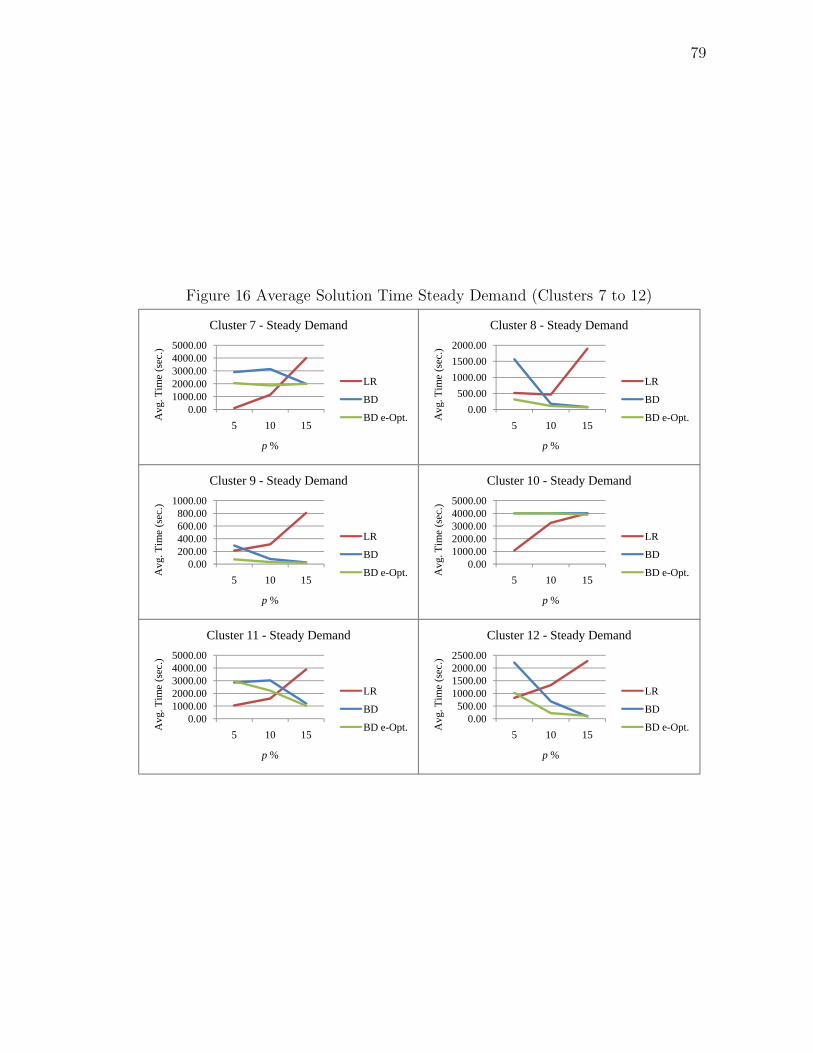
79

Figure 16 Average Solution Time Steady Demand (Clusters 7 to 12)

Cluster 7 - Steady Demand Cluster 8 - Steady Demand

0.001000.002000.003000.004000.005000.00

5 10 15

Avg

. Tim

e (s

ec.)

LR

BD

BD e-Opt.0.00

500.001000.001500.002000.00

5 10 15A

vg. T

ime

(sec

.)

LR

BD

BD e-Opt.

p % p %

600.00800.00

1000.00

e (s

ec.)

Cluster 9 - Steady Demand

LR3000.004000.005000.00

e (s

ec.)

Cluster 10 - Steady Demand

0.00200.00400.00

5 10 15

Avg

. Tim

e

p %

LR

BD

BD e-Opt.0.00

1000.002000.00

5 10 15

Avg

. Tim

e

p %

LR

BD

BD e-Opt.

Cl 11 S d D d Cl 12 S d D d

0.001000.002000.003000.004000.005000.00

Avg

. Tim

e (s

ec.)

Cluster 11 - Steady Demand

LR

BD

BD e-Opt.0.00

500.001000.001500.002000.002500.00

Avg

. Tim

e (s

ec.)

Cluster 12 - Steady Demand

LR

BD

BD e-Opt.5 10 15

A

p %

BD e Opt.5 10 15

A

p %

BD e Opt.

80

IV.5. Summary and Conclusions

In this chapter we described the DCFLP and presented a mixed integer programming

formulation. We developed a Lagrangian relaxation and Benders’ decomposition al-

gorithms to solve the model. Both algorithms showed to be more efficient compared

with conventional branch and cut in solving classes of problems for each total demand

structure. We observed that the efficiency of the solution algorithms depends on the

cost structure and demand pattern considered. Lagrangian relaxation performed bet-

ter for classes of problems with a smaller number of open facilities, and for classes

where the fixed operation cost represents 50−65% of the average total cost. Benders’

decomposition performed better for classes of problems with a larger number of open

facilities and for classes of problems where the cost split of the average total cost

considered 70 − 85% of fixed operation costs. The ε-optimal algorithm performed

better for classes of problems with total decreasing demand, in particular for small

size problems and classes with a cost split of 70− 80% for fixed operation cost.

81

CHAPTER V

DYNAMIC DEMAND CAPACITATED FIXED CHARGE LOCATION

PROBLEM WITHOUT RELOCATION (DDCFLP)

In this chapter, we investigate the problem of finding the locations of facilities with

limited capacity to satisfy the demand of a set of customers over a discrete and finite

time horizon when relocation of facilities is not allowed. The demand of each customer

is assumed to be time varying (in a known way) and can be split or served by one

or more facilities. There are fixed costs associated with establishing or opening new

facilities and for operating the facilities. Also, there is a variable transportation cost

for serving the demand of customers. The main objective is to find an optimal set of

locations for facilities to satisfy the time varying demand while observing the capacity

restrictions over the time horizon.

The chapter is organized as follows. In Section V.1, we give the problem state-

ment. Section V.2, presents the mixed integer programming formulation and notation

for the DDCFLP. In Section V.3, we develop a Benders’ decomposition algorithm to

solve the DDCFLP. In Section V.4, we present numerical results using different total

demand patterns to test the performance of the solution algorithm. In Section V.5,

we show that when relocation costs (for opening and closing facilities) are consider-

ably large, the DDCFLP can be solved as a special case using the DCFLP model.

Finally, in Section V.6, we summarize the results and give concluding remarks.

V.1. Problem Statement

The DDCFLP statement is as follows. Consider a geographical region where a given

group of customers are dispersed. Each customer has a given demand for a certain

82

product. Along a discrete and finite time horizon, the total demand of the customers

is time varying in a known way.

The establishment of facilities is required to supply the demand of customers over

the entire time horizon. Each facility has a limit or capacity in the amount of demand

that can be supplied to the customers. Each customer can be supplied by one or more

facilities. The shipments of demand between facilities and customers incur a variable

transportation cost proportional to quantity and distance. Further, the establishment

of a new facility incurs a fixed opening cost, which can represent the initial investment

for construction, equipment, and resources needed to start operations. An additional

fixed operation cost is incurred in each period the facility remains operational; this

can be thought of as the per period cost associated with the initial investment or the

total expenses for services and labors. Establishment of facilities takes place at once

in the beginning of the time horizon and can not be closed or relocated.

The main decisions are determining the number of facilities required to supply

the demand, selecting the locations to establish the facilities at the beginning of the

time horizon, and allocating demand to facilities in such a way that the total fixed

and variable costs are minimal without exceeding the capacity of facilities over the

entire time horizon.

V.2. Model and Notation

In this section, we provide a mixed integer programming formulation of the DDCFLP.

We use the following notation.

Parameters

I set of demand locations, i = 1, . . . , n

J set of facility locations, j = 1, . . . , m

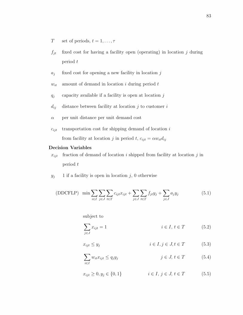
83

T set of periods, t = 1, . . . , τ

fjt fixed cost for having a facility open (operating) in location j during

period t

aj fixed cost for opening a new facility in location j

wit amount of demand in location i during period t

qj capacity available if a facility is open at location j

dij distance between facility at location j to customer i

α per unit distance per unit demand cost

cijt transportation cost for shipping demand of location i

from facility at location j in period t, cijt = αwitdij

Decision Variables

xijt fraction of demand of location i shipped from facility at location j in

period t

yj 1 if a facility is open in location j, 0 otherwise

(DDCFLP) min∑i∈I

∑j∈J

∑t∈T

cijtxijt +∑j∈J

∑t∈T

fjtyj +∑j∈J

ajyj (5.1)

subject to∑j∈J

xijt = 1 i ∈ I, t ∈ T (5.2)

xijt ≤ yj i ∈ I, j ∈ J, t ∈ T (5.3)

∑i∈I

witxijt ≤ qjyj j ∈ J, t ∈ T (5.4)

xijt ≥ 0, yj ∈ {0, 1} i ∈ I, j ∈ J, t ∈ T (5.5)

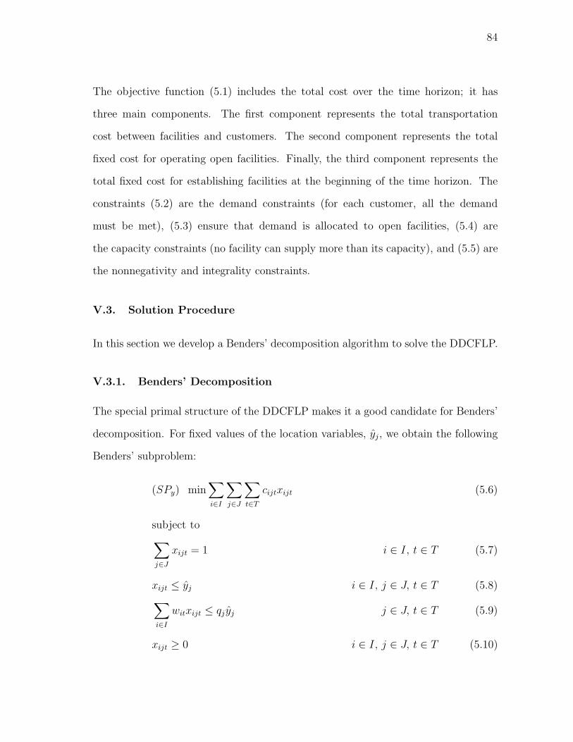
84

The objective function (5.1) includes the total cost over the time horizon; it has

three main components. The first component represents the total transportation

cost between facilities and customers. The second component represents the total

fixed cost for operating open facilities. Finally, the third component represents the

total fixed cost for establishing facilities at the beginning of the time horizon. The

constraints (5.2) are the demand constraints (for each customer, all the demand

must be met), (5.3) ensure that demand is allocated to open facilities, (5.4) are

the capacity constraints (no facility can supply more than its capacity), and (5.5) are

the nonnegativity and integrality constraints.

V.3. Solution Procedure

In this section we develop a Benders’ decomposition algorithm to solve the DDCFLP.

V.3.1. Benders’ Decomposition

The special primal structure of the DDCFLP makes it a good candidate for Benders’

decomposition. For fixed values of the location variables, yj, we obtain the following

Benders’ subproblem:

(SPy) min∑i∈I

∑j∈J

∑t∈T

cijtxijt (5.6)

subject to∑j∈J

xijt = 1 i ∈ I, t ∈ T (5.7)

xijt ≤ yj i ∈ I, j ∈ J, t ∈ T (5.8)∑i∈I

witxijt ≤ qj yj j ∈ J, t ∈ T (5.9)

xijt ≥ 0 i ∈ I, j ∈ J, t ∈ T (5.10)

85

And the associated dual of the subproblem:

(DSPy) max∑i∈I

∑t∈T

λit −∑i∈I

∑j∈J

∑t∈T

yjμijt −∑j∈J

∑t∈T

qj yjγjt (5.11)

subject to

λit − μijt − witγjt ≤ cijt i ∈ I, j ∈ J, t ∈ T (5.12)

λit unrestricted, μijt ≥ 0, γjt ≥ 0 i ∈ I, j ∈ J, t ∈ T (5.13)

which can be further decomposed into |T | independent dual subproblems (one for

each period t ∈ T ). Since the feasible region of the primal subproblem is non-empty

and bounded, we do not need to consider the extreme rays of the feasible region of

the dual subproblem.

We have the following Benders’ master problem:

(MPK) min ρ +∑j∈J

∑t∈T

fjtyj +∑j∈J

ajyj (5.14)

subject to

ρ ≥∑i∈I

∑t∈T

λkit −

∑i∈I

∑j∈J

∑t∈T

μkijtyj −

∑j∈J

∑t∈T

qjγkjtyj k ∈ K ⊆ P (5.15)

∑i∈I

wit ≤∑j∈J

qjyj t ∈ T (5.16)

ρ ≥ 0, yj ∈ {0, 1} j ∈ J (5.17)

where{(λk, μk, γk) : k ∈ P

}denote all the extreme points of (DSPy), K is an appro-

priate index set, and ρ denotes the objective function value of the dual subproblem.

We can let ρ ≥ 0 provided that cijt ≥ 0. Adding the surrogate constraints (5.16) to

the master problem guarantees that any solution to the master problem is a feasible

86

solution (with enough capacity) for the primal and dual subproblems.

The number of extreme points of the dual subproblem can be very large, thus

increasing the size and computational effort to solve the master problem. Observe

that, in an optimal solution to the master problem, only a small subset of constraints

(5.15) will be binding. Thus, we can consider only a subset of these constraints.

Clearly, this relaxed master problem gives a lower bound on the optimal objective

function value of the DDCFLP.

An upper bound can be obtained for fixed values of the location variables, yj,

obtained from the solution to the master problem, solving the following transportation

problem:

(TPy) min∑i∈I

∑j∈J

∑t∈T

cijtxijt +∑j∈J

∑t∈T

fjtyj +∑j∈J

aj yj (5.18)

subject to∑j∈J

xijt = 1 i ∈ I, t ∈ T (5.19)

∑i∈I

witxijt ≤ qj yj j ∈ J, t ∈ T (5.20)

xijt ≥ 0 i ∈ I, j ∈ J, t ∈ T (5.21)

V.3.1.1. Generation of Strong Cuts

It is known that the Benders’ subproblem (transportation problem) has a high level

of degeneracy, thus the dual subproblem can have alternative optimal solutions. Since

the improvement in the value of the lower bound (obtained from the solution to the

relaxed master problem) is tightened by the Benders’ cuts obtained from the dual

subproblem, it is important that at each iteration of the decomposition procedure we

87

select the best possible cut.

To strengthen the Benders’ cuts obtained from the dual subproblem, we imple-

ment the algorithm proposed by Van Roy (1986). The values of the dual variables

μijt and γjt can be improved without affecting the objective function value of the dual

subproblem for the closed facilities. Let C = {j ∈ J : yj = 0} denote the set of closed

facilities, and O = {j ∈ J : yj = 1} the set of open facilities. Also let j(i)t denote the

allocation of customer location i to candidate location j in period t, obtained from

an optimal solution to (SPy). Let (λit, μijt, γjt) denote the value of the optimal dual

variables obtained from the dual subproblem (DSPy). We set yj = 1, j ∈ C, then

solve the following linear program:

(SCy) max−∑i∈I

∑j∈J

∑t∈T

μijtyj −∑j∈J

∑t∈T

qj γjtyj (5.22)

subject to

λit − μijt − witγjt ≤ cijt i ∈ I, j ∈ J, t ∈ T (5.23)

μijt ≥ 0, γjt ≥ 0 i ∈ I, j ∈ J, t ∈ T (5.24)

From the optimal solution to (SCy), we set μijt = μijt, γjt = γjt, j ∈ C, and leave

the previous values of the dual variables, μijt, γjt, j ∈ O, unchanged. Note that,

constraints (5.23) guarantee that (λjt, μijt, γjt) is a feasible solution to the dual sub-

problem.

V.3.1.2. Generation of Pareto-Optimal Cuts

The generation of strong cuts produces significant savings in computation time for

the decomposition procedure. However, we can further improve the Benders’ cuts by

considering the closed and open facilities. This procedure relies on the concept of

88

pareto-optimal cuts introduced by Magnanti and Wong (1981). The main idea is to

generate a cut that dominates any other cut, that is, a constraint which is tighter

than any other. This is called a pareto-optimal cut.

Wentges (1996) developed an algorithm to generate pareto-optimal cuts for the

CFLP by considering the open and closed facilities. Observe that, from the relation-

ship between the primal and dual subproblems, the value of the dual variables λit

represents the cost for serving demand of customer i in period t, and the value of

the dual variables μijt the cost for allocating costumer i to facility j in period t. The

fair cost that customer i should pay for being served by facility j(i), which is closer

and more convenient, can be thought of as the additional cost for being served by

the second nearest facility. Thus, for the open facilities we can increase the value of

λit and γjt, and decrease the cost (or give a reward) of μij(i)t. In doing so, the objec-

tive function value of the dual subproblem remains unchanged and also constraints

(5.12) are satisfied. However, the improvement on the value of the dual variables λit

could be too high since the closed facilities are not considered. It is possible that

customer i could be better served by one of the closed facilities. Thus, in addition

to the open facilities we can improve the value of the dual variables considering the

closed facilities.

The algorithm to develop pareto-optimal cuts improves the values of the dual

variables by considering both the open and closed facilities. The additional service

cost for the open facilities is determined between the first and second smallest costs

in the set {cijt+ γjt : j ∈ O}. Note that if xijt happens to be in the basis of the primal

subproblem, then λit = cij(i)t + γj(i)t, for some j(i)t ∈ O (complementary slackness).

In selecting the additional service cost for the closed facilities we selected the third

smallest value in the set {cijt + γjt : j ∈ C} as it gave the best improvement in the

efficiency of the Benders’ decomposition algorithm.

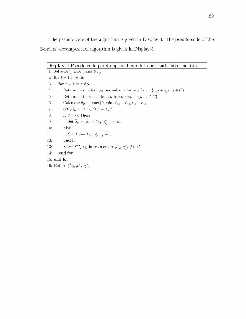
89

The pseudo-code of the algorithm is given in Display 4. The pseudo-code of the

Benders’ decomposition algorithm is given in Display 5.

Display 4 Pseudo-code pareto-optimal cuts for open and closed facilities1: Solve SPy, DSPy and SCy

2: for i = 1 to n do

3: for t = 1 to τ do

4: Determine smallest ψit, second smallest φit from: {cijt + γjt : j ∈ O}5: Determine third smallest �it from: {cijt + γjt : j ∈ C}6: Calculate θit ← max {0,min {φit − ψit, �it − ψit}}7: Set μ∗

ijt ← 0 j ∈ O, j �= j(i)t

8: if θit > 0 then

9: Set λit ← λit + θit, μ∗ij(i)← θit

10: else

11: Set λit ← λit, μ∗ij(i)t

← 0

12: end if

13: Solve SCy again to calculate μ∗ijt, γ

∗jt, j ∈ C

14: end for

15: end for

16: Return (λit, μ∗ijt, γ

∗jt)

90

Display 5 Pseudo-code Benders’ decomposition algorithm1: Initialize: k ← 0, ZLB ← −∞, ZUB ←∞2: Solve MPK

3: Zklb ←MPK

4: if Zklb > ZLB then

5: ZLB ← Zklb

6: end if

7: while k ≤ M do

8: Solve DSPy

9: Set: Zkub ← DSPy + fixed costs

10: if Zkub < ZUB then

11: ZUB ← Zkub

12: Record S

13: end if

14: if (ZUB − ZLB)/ZUB ≤ ε then

15: Stop

16: else

17: Obtain pareto-optimal cut: (λit, μ∗ijt, γ

∗jt)

18: Solve MPK with (λit, μ∗ijt, γ

∗jt)

19: Set: Zklb ←MPK

20: if Zklb > ZLB then

21: ZLB ← Zklb

22: end if

23: if (ZUB − ZLB)/ZUB ≤ ε then

24: Stop

25: end if

26: end if

27: k ← k + 1

28: end while

29: Return S,ZUB

V.4. Numerical Results

In this section we conduct a numerical experiment to test the performance of the

decomposition algorithm developed for the DDCFLP. We designed 72 classes of prob-

lems considering three total demand structures, increasing, decreasing, and steady;

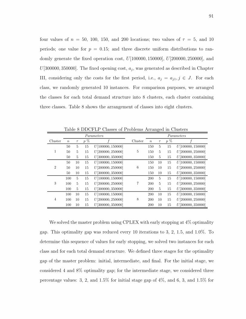
91

four values of n = 50, 100, 150, and 200 locations; two values of τ = 5, and 10

periods; one value for p = 0.15; and three discrete uniform distributions to ran-

domly generate the fixed operation cost, U [100000, 150000], U [200000, 250000], and

U [300000, 350000]. The fixed opening cost, aj , was generated as described in Chapter

III, considering only the costs for the first period, i.e., aj = aj1, j ∈ J . For each

class, we randomly generated 10 instances. For comparison purposes, we arranged

the classes for each total demand structure into 8 clusters, each cluster containing

three classes. Table 8 shows the arrangement of classes into eight clusters.

Table 8 DDCFLP Classes of Problems Arranged in Clusters

Parameters ParametersCluster n τ p % f Cluster n τ p % f

150 5 15 U [100000, 150000]

5150 5 15 U [100000, 150000]

50 5 15 U [200000, 250000] 150 5 15 U [200000, 250000]50 5 15 U [300000, 350000] 150 5 15 U [300000, 350000]

250 10 15 U [100000, 150000]

6150 10 15 U [100000, 150000]

50 10 15 U [200000, 250000] 150 10 15 U [200000, 250000]50 10 15 U [300000, 350000] 150 10 15 U [300000, 350000]

3100 5 15 U [100000, 150000]

7200 5 15 U [100000, 150000]

100 5 15 U [200000, 250000] 200 5 15 U [200000, 250000]100 5 15 U [300000, 350000] 200 5 15 U [300000, 350000]

4100 10 15 U [100000, 150000]

8200 10 15 U [100000, 150000]

100 10 15 U [200000, 250000] 200 10 15 U [200000, 250000]100 10 15 U [300000, 350000] 200 10 15 U [300000, 350000]

We solved the master problem using CPLEX with early stopping at 4% optimality

gap. This optimality gap was reduced every 10 iterations to 3, 2, 1.5, and 1.0%. To

determine this sequence of values for early stopping, we solved two instances for each

class and for each total demand structure. We defined three stages for the optimality

gap of the master problem: initial, intermediate, and final. For the initial stage, we

considered 4 and 8% optimality gap; for the intermediate stage, we considered three

percentage values: 3, 2, and 1.5% for initial stage gap of 4%, and 6, 3, and 1.5% for

92

initial stage gap of 8%. For the final stage, we considered a percentage gap of 1.0%.

For the number of iterations, we considered 5, 10, and 15 iterations. We selected the

combination that gave the lowest average optimality gap and lowest average solution

time over all the classes.

At each iteration of the decomposition algorithm, we solved the master problem

using CPLEX, with early stopping as described above. We took the lower bound value

from the solution given by CPLEX and set it as the trial lower bound. To compute

the upper bound, the set of open facilities obtained from the master problem was

given as an input to CPLEX to solve |T | dual problems to optimality. The value of

the trial upper bound at iteration k was computed by Zkub = DSPy plus the associated

fixed costs. The primal subproblem and the strong-cuts algorithm were also solved

using CPLEX. The stopping criteria for the Benders’ decomposition algorithms was

set to 1.5% optimality gap and M = 200 iterations.

The benchmark solutions were obtained solving the DDCFLP model with CPLEX,

which uses a branch and cut algorithm, using default settings. We used early stopping

with an optimality gap of 1.5%, and recorded the lower and upper bound values.

For all the experiments, we limited the running time for each instance with n = 50

to 3000 seconds, n = 100 to 4000 seconds, n = 150 to 5000 seconds, and n = 200

to 6000 seconds. For each class, we reported the average and maximum value of the

optimality gap and the average and maximum solution time. Tables 9, 10, and 11 on

pages 95, 96, and 97 respectively, describe the performance of the solution algorithms

for each total demand structure. We denote by NS the benchmark classes Not Solved

by CPLEX within the maximum solution time.

In the analysis, we considered the cost split, in percentage value, of the total cost

corresponding to variable transportation cost and fixed opening, operation, and clos-

ing costs. For each class, we selected the solution with minimum average optimality

93

gap to compute the average percentage for each type of cost. Tables 12, 13, and 14

on pages 98, 99, and 100 respectively, report the average cost split per class for each

total demand structure, and the average number of open facilities. The analysis of

the cost split is important to identify a possible relationship between the efficiency of

the solution algorithm and the structure of the cost split for each class of problems.

From Tables 9, 10, and 11 on pages 95, 96, and 97 respectively, we see that

Benders’ decomposition is shown to be more efficient in solving the DDCFLP than

the branch and cut procedure used by CPLEX. For the three demand structures, the

decomposition algorithm required less solution time on average.

For classes with increasing and steady demand, we observe on pages 95 and

97 in Tables 9 and 11 respectively, that increasing the value of the fixed operation

cost decreases the average solution time of Benders’ decomposition algorithm. The

reason for this can be explained by looking into the structure of the master problem.

The three main components in the objective function of the master problem are the

fixed operation cost, fixed opening cost, and the auxiliary variable associated with

the dual subproblem that considers the total transportation cost. For increasing

demand, a larger number of facilities is expected to be established in the first period

and remain operational along the time horizon. Since the largest demand is expected

to be in the last period, the set of open facilities carries over some extra capacity

that is eventually used as demand increases. Thus, the main contribution to the

objective function value comes from the facility fixed costs. Since the upper bound

value incorporates these costs, plus the additional variable transportation costs which

gradually become larger, the optimality gap between the relaxed master problem and

primal subproblem diminishes quickly. From Table 12 on page 98 we observe that for

increasing demand the average solution time of Benders’ decomposition is smaller for

classes with an average cost split of 80 − 85% of fixed operation cost. The average

94

number of facilities for each class is near the expected number of open facilities,

pm. Note that, for increasing demand, as we increase the fixed operation cost the

average number of open facilities remains the same. Also, the average number of

facilities tends to be located in regions B and C, since demand is shifting towards

these regions.

For classes with steady demand, the fixed costs represent the main portion of the

objective function value, as we observe from Table 11 on page 97. In these classes, the

solution to the master problem takes more time than classes with increasing demand.

Since demand is fluctuating, the set of open facilities tends to be determined by the

locations where the average total demand concentrates over the time horizon. We

see from Table 14 on page 100, that the average number of open facilities is larger in

regions B and C.

For the classes with decreasing demand, we observe from Table 10 on page 96

that in general the average solution time is smaller than the average time taken

to solve problems with increasing and steady demand. Furthermore, we observe in

this case that increasing the fixed operation cost does not have a significant impact

on the average solution time. However, increasing the problem size, specially the

number of periods, seems to increase the average solution time. Observe that, the

main contribution to the objective function value comes from the fixed costs since

the transportation cost is decreasing, thus the optimality gap is closed faster. From

Table 13 on page 99, we see that Benders’ decomposition takes less average solution

time for classes with an average cost split with 80 − 90% of fixed operation cost.

Note that in this case, since demand is decreasing, the percentage in the cost split for

fixed operation cost is higher than the split for increasing demand. Further, notice

that the average number of open facilities is larger in regions A and B. Since demand

in decreasing, the open facilities will have to serve regions with the higher levels of

95

Table 9 DDCFLP Computational Results Increasing Demand

Branch & Cut Benders’ DecompositionGap (%) Time (sec.) Gap (%) Time (sec.)

Cluster Avg. Max. Avg. Max. Avg. Max. Avg. Max.

12.10 5.74 983.04 3000.28 1.34 1.48 6.00 12.412.92 8.59 912.23 3000.58 1.22 1.39 5.83 23.453.25 9.82 912.04 3000.43 1.19 1.49 6.74 22.97

21.53 6.39 934.08 3000.22 1.22 1.48 19.47 30.440.56 1.25 131.91 760.16 1.22 1.45 6.87 30.950.69 1.50 159.41 923.63 1.29 1.47 4.40 23.94

30.59 1.02 587.66 3550.08 1.46 1.49 19.00 53.331.00 1.49 328.13 423.27 1.25 1.49 25.10 68.241.13 1.50 715.77 1761.55 1.15 1.49 20.39 72.83

41.88 3.93 2314.47 4000.58 1.45 1.49 160.99 302.191.14 5.10 1671.21 4000.44 1.36 1.49 43.50 137.791.39 5.46 1921.63 4000.33 1.41 1.49 21.26 43.06

50.88 3.24 2041.50 5000.34 1.36 1.47 82.21 199.580.67 1.33 1599.20 2219.89 1.43 1.50 23.66 35.410.93 1.43 2607.74 3849.98 1.24 1.49 24.12 68.47

6NS NS NS NS 1.43 1.50 786.02 3280.98NS NS NS NS 1.41 1.50 153.26 508.01NS NS NS NS 1.22 1.48 113.73 301.22

70.60 1.90 3515.96 6000.52 1.36 1.47 490.50 3701.36NS NS NS NS 1.28 1.50 136.21 364.38NS NS NS NS 1.28 1.50 121.73 384.14

8NS NS NS NS 1.42 1.49 736.69 1350.70NS NS NS NS 1.35 1.50 262.68 605.00NS NS NS NS 1.09 1.48 591.32 1497.94

demand.

96

Table 10 DDCFLP Computational Results Decreasing Demand

Branch & Cut Benders’ DecompositionGap (%) Time (sec.) Gap (%) Time (sec.)

Cluster Avg. Max. Avg. Max. Avg. Max. Avg. Max.

12.56 7.36 924.47 3000.36 1.30 1.44 2.73 7.863.17 9.72 906.98 3000.34 0.99 1.38 3.69 13.243.57 10.94 906.35 3000.27 0.94 1.49 5.97 25.84

21.26 1.38 214.19 3000.33 1.28 1.46 4.65 16.560.74 1.38 66.21 83.69 1.23 1.49 1.71 3.690.81 1.49 73.71 123.02 1.21 1.48 4.68 32.78

31.49 1.87 520.62 4000.80 1.16 1.49 11.70 55.731.22 1.50 1338.19 3766.56 1.06 1.48 21.01 58.771.36 1.79 1900.72 4000.47 1.00 1.46 24.31 70.39

41.86 5.18 1663.55 4000.53 1.28 1.50 22.76 74.331.66 6.24 2440.01 4000.47 1.26 1.48 17.39 104.911.09 1.91 2477.76 4000.56 1.26 1.50 19.22 131.10

51.31 3.93 3110.19 5000.56 1.29 1.48 21.09 34.090.80 1.50 2028.26 3190.67 1.24 1.48 9.54 28.931.04 1.68 2665.06 5000.50 1.21 1.49 10.00 22.92

6NS NS NS NS 1.35 1.49 91.79 443.52NS NS NS NS 1.25 1.50 49.28 95.64NS NS NS NS 1.09 1.45 90.99 351.17

7NS NS NS NS 1.32 1.46 81.67 316.72NS NS NS NS 1.28 1.49 74.73 412.61NS NS NS NS 1.27 1.50 67.66 359.41

8NS NS NS NS 1.40 1.50 171.02 396.34NS NS NS NS 1.31 1.49 212.49 721.72NS NS NS NS 1.05 1.49 315.17 974.33

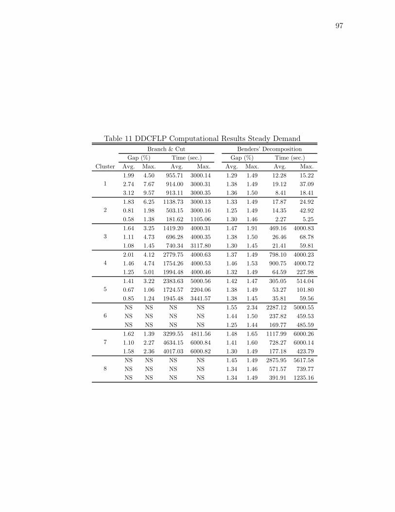
97

Table 11 DDCFLP Computational Results Steady Demand

Branch & Cut Benders’ DecompositionGap (%) Time (sec.) Gap (%) Time (sec.)

Cluster Avg. Max. Avg. Max. Avg. Max. Avg. Max.

11.99 4.50 955.71 3000.14 1.29 1.49 12.28 15.222.74 7.67 914.00 3000.31 1.38 1.49 19.12 37.093.12 9.57 913.11 3000.35 1.36 1.50 8.41 18.41

21.83 6.25 1138.73 3000.13 1.33 1.49 17.87 24.920.81 1.98 503.15 3000.16 1.25 1.49 14.35 42.920.58 1.38 181.62 1105.06 1.30 1.46 2.27 5.25

31.64 3.25 1419.20 4000.31 1.47 1.91 469.16 4000.831.11 4.73 696.28 4000.35 1.38 1.50 26.46 68.781.08 1.45 740.34 3117.80 1.30 1.45 21.41 59.81

42.01 4.12 2779.75 4000.63 1.37 1.49 798.10 4000.231.46 4.74 1754.26 4000.53 1.46 1.53 900.75 4000.721.25 5.01 1994.48 4000.46 1.32 1.49 64.59 227.98

51.41 3.22 2383.63 5000.56 1.42 1.47 305.05 514.040.67 1.06 1724.57 2204.06 1.38 1.49 53.27 101.800.85 1.24 1945.48 3441.57 1.38 1.45 35.81 59.56

6NS NS NS NS 1.55 2.34 2287.12 5000.55NS NS NS NS 1.44 1.50 237.82 459.53NS NS NS NS 1.25 1.44 169.77 485.59

71.62 1.39 3299.55 4811.56 1.48 1.65 1117.99 6000.261.10 2.27 4634.15 6000.84 1.41 1.60 728.27 6000.141.58 2.36 4017.03 6000.82 1.30 1.49 177.18 423.79

8NS NS NS NS 1.45 1.49 2875.95 5617.58NS NS NS NS 1.34 1.46 571.57 739.77NS NS NS NS 1.34 1.49 391.91 1235.16

98

Table 12 Average Cost Split and Open Facilities for Increasing Demand

Cost Split (%) Open FacilitiesCluster Transportation Operation Opening Avg. A B C

116.36 71.25 12.39 6.3 1.9 2.2 2.29.49 77.67 12.84 6.3 1.9 2.2 2.26.85 80.05 13.10 6.3 1.9 2.1 2.3

222.24 71.58 6.18 6.0 2.0 1.7 2.312.89 80.47 6.64 6.0 2.1 1.6 2.39.37 83.77 6.86 6.0 2.0 1.8 2.2

312.45 74.62 12.93 13.0 4.3 4.2 4.57.34 79.49 13.17 13.0 4.3 4.1 4.65.21 81.52 13.27 13.0 4.0 4.5 4.5

415.80 77.48 6.72 13.0 4.3 4.2 4.59.48 83.66 6.87 13.0 3.9 4.2 4.96.75 86.22 7.03 13.0 3.6 4.5 4.9

511.22 75.62 13.16 19.0 6.1 6.1 6.86.40 80.30 13.30 19 6.1 6.3 6.64.50 82.12 13.38 19.0 5.8 6.5 6.7

614.01 79.17 6.81 19.0 5.2 6.2 7.68.34 84.66 7.00 19.0 5.2 6.6 7.25.78 87.08 7.14 19.0 5.3 6.2 7.5

79.84 76.77 13.39 26.1 5.2 6.2 7.65.70 80.93 13.36 26.0 8.7 8.4 8.94.00 82.54 13.46 26.0 8.2 8.9 8.9

812.40 80.62 6.98 26.0 7.1 8.5 10.47.38 85.52 7.10 26.0 6.7 9.1 10.25.27 87.60 7.13 26.0 7.0 8.7 10.3

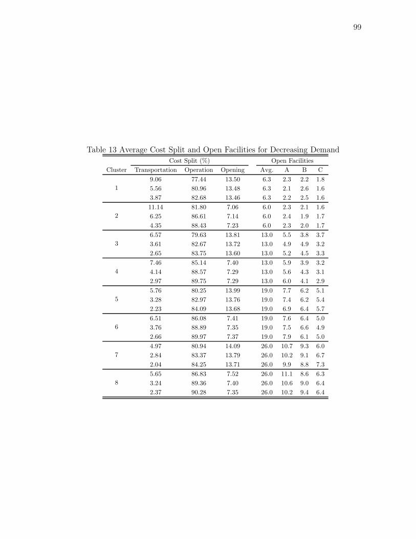
99

Table 13 Average Cost Split and Open Facilities for Decreasing Demand

Cost Split (%) Open FacilitiesCluster Transportation Operation Opening Avg. A B C

19.06 77.44 13.50 6.3 2.3 2.2 1.85.56 80.96 13.48 6.3 2.1 2.6 1.63.87 82.68 13.46 6.3 2.2 2.5 1.6

211.14 81.80 7.06 6.0 2.3 2.1 1.66.25 86.61 7.14 6.0 2.4 1.9 1.74.35 88.43 7.23 6.0 2.3 2.0 1.7

36.57 79.63 13.81 13.0 5.5 3.8 3.73.61 82.67 13.72 13.0 4.9 4.9 3.22.65 83.75 13.60 13.0 5.2 4.5 3.3

47.46 85.14 7.40 13.0 5.9 3.9 3.24.14 88.57 7.29 13.0 5.6 4.3 3.12.97 89.75 7.29 13.0 6.0 4.1 2.9

55.76 80.25 13.99 19.0 7.7 6.2 5.13.28 82.97 13.76 19.0 7.4 6.2 5.42.23 84.09 13.68 19.0 6.9 6.4 5.7

66.51 86.08 7.41 19.0 7.6 6.4 5.03.76 88.89 7.35 19.0 7.5 6.6 4.92.66 89.97 7.37 19.0 7.9 6.1 5.0

74.97 80.94 14.09 26.0 10.7 9.3 6.02.84 83.37 13.79 26.0 10.2 9.1 6.72.04 84.25 13.71 26.0 9.9 8.8 7.3

85.65 86.83 7.52 26.0 11.1 8.6 6.33.24 89.36 7.40 26.0 10.6 9.0 6.42.37 90.28 7.35 26.0 10.2 9.4 6.4

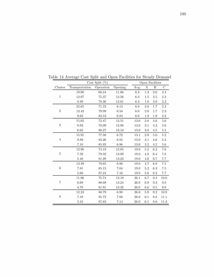
100

Table 14 Average Cost Split and Open Facilities for Steady Demand

Cost Split (%) Open FacilitiesCluster Transportation Operation Opening Avg. A B C

119.90 68.24 11.86 6.3 1.3 2.6 2.412.07 75.37 12.56 6.3 1.5 2.5 2.38.89 78.30 12.81 6.3 1.0 3.0 2.3

222.65 71.22 6.13 6.0 2.0 1.7 2.313.42 79.99 6.58 6.0 2.0 1.7 2.39.63 83.53 6.84 6.0 1.9 1.9 2.2

315.02 72.47 12.51 13.0 2.8 4.6 5.68.93 78.09 12.98 13.0 3.1 4.3 5.66.63 80.27 13.10 13.0 3.0 4.5 5.5

415.91 77.38 6.72 13.1 2.9 5.0 5.29.89 83.26 6.85 13.0 3.1 4.6 5.37.10 85.92 6.98 13.0 3.2 4.2 5.6

512.96 74.19 12.85 19.0 5.2 6.2 7.67.59 79.32 13.09 19.0 4.8 6.4 7.85.48 81.29 13.23 19.0 4.6 6.7 7.7

613.49 79.65 6.86 19.0 4.7 6.8 7.57.81 85.15 7.04 19.0 5.2 6.3 7.55.60 87.24 7.16 19.0 5.0 6.3 7.7

711.06 75.74 13.19 26.1 6.7 9.4 10.06.68 80.08 13.24 26.0 6.9 9.3 9.84.78 81.91 13.32 26.0 6.6 9.5 9.9

812.23 80.79 6.98 26.0 5.9 9.2 10.97.19 85.72 7.08 26.0 6.1 8.8 11.15.24 87.62 7.14 26.0 6.1 8.6 11.3

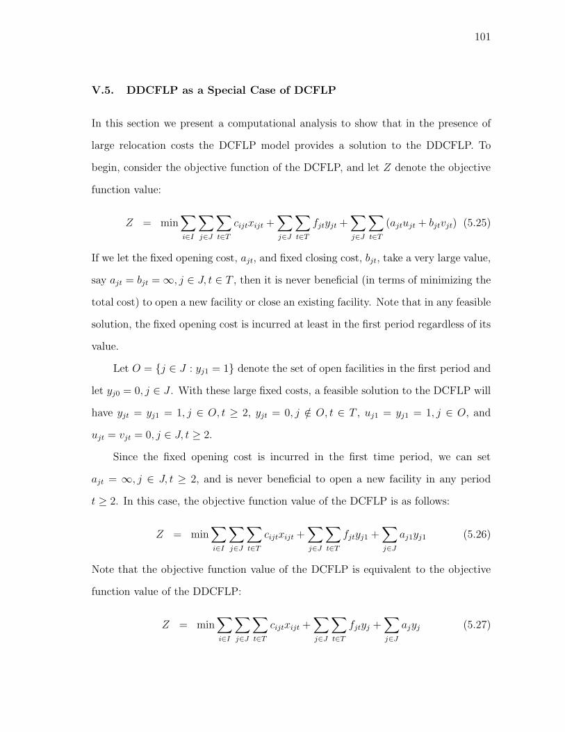
101

V.5. DDCFLP as a Special Case of DCFLP

In this section we present a computational analysis to show that in the presence of

large relocation costs the DCFLP model provides a solution to the DDCFLP. To

begin, consider the objective function of the DCFLP, and let Z denote the objective

function value:

Z = min∑i∈I

∑j∈J

∑t∈T

cijtxijt +∑j∈J

∑t∈T

fjtyjt +∑j∈J

∑t∈T

(ajtujt + bjtvjt) (5.25)

If we let the fixed opening cost, ajt, and fixed closing cost, bjt, take a very large value,

say ajt = bjt =∞, j ∈ J, t ∈ T , then it is never beneficial (in terms of minimizing the

total cost) to open a new facility or close an existing facility. Note that in any feasible

solution, the fixed opening cost is incurred at least in the first period regardless of its

value.

Let O = {j ∈ J : yj1 = 1} denote the set of open facilities in the first period and

let yj0 = 0, j ∈ J . With these large fixed costs, a feasible solution to the DCFLP will

have yjt = yj1 = 1, j ∈ O, t ≥ 2, yjt = 0, j /∈ O, t ∈ T , uj1 = yj1 = 1, j ∈ O, and

ujt = vjt = 0, j ∈ J, t ≥ 2.

Since the fixed opening cost is incurred in the first time period, we can set

ajt = ∞, j ∈ J, t ≥ 2, and is never beneficial to open a new facility in any period

t ≥ 2. In this case, the objective function value of the DCFLP is as follows:

Z = min∑i∈I

∑j∈J

∑t∈T

cijtxijt +∑j∈J

∑t∈T

fjtyj1 +∑j∈J

aj1yj1 (5.26)

Note that the objective function value of the DCFLP is equivalent to the objective

function value of the DDCFLP:

Z = min∑i∈I

∑j∈J

∑t∈T

cijtxijt +∑j∈J

∑t∈T

fjtyj +∑j∈J

ajyj (5.27)

102

Clearly, with this setting for relocation costs a feasible solution to the DCFLP is

also feasible for the DDCFLP. Thus, we should question the need for a mixed integer

programming model to solve the DDCFLP if we can use the DCFLP model, with

special input data modifications, instead. In other words, is the DDCFLP model

necessary? The answer is, yes.

It is possible to develop different formulations for an optimization problem such as

the DDCFLP. However, a particular formulation will be preferred among the others.

This ideal formulation will be the one that provides the tightest formulation since

this can affect the performance of the solution method. A weak formulation will

have a very large feasible region, making it too time consuming to explore. On the

other hand, a strong formulation will have a very tight feasible region, taking less

computational effort to be explored.

We can think of the DCFLP as the weak formulation since it has a larger num-

ber of variables and constraints, most of them taking zero value, and the DDCFLP

model as the strong formulation. Thus, we would expect that the performance of any

solution algorithm will be more efficient in solving the DDCFLP model than solving

the DCFLP with special input data.

To support this claim, we conducted a numerical experiment consisting of 18

classes of problems using three total demand structures described in Chapter III,

increasing, decreasing, and steady; three values for n = 50, 100, and 150 locations; two

values for τ = 5 and 10 periods; p = 0.15; and a single discrete uniform distribution,

U [300000, 350000], to generate the fixed operation cost. For the DCFLP, we set

ajk = bjk = 700 × 106, j ∈ J, t ∈ T, k ≥ 2. For the DDCFLP, fixed opening cost

considered only the costs for the first period, i.e., aj = aj1, j ∈ J . Table 15 shows the

arrangement of classes into six clusters.

103

Table 15 Classes of Problems Arranged in Clusters

Parameters ParametersCluster n τ p % f Cluster n τ p % f

1 50 5 15 U [300000, 350000] 4 50 10 15 U [300000, 350000]2 100 5 15 U [300000, 350000] 5 100 10 15 U [300000, 350000]3 150 5 15 U [300000, 350000] 6 150 10 15 U [300000, 350000]

We used the corresponding implementation of Benders’ decomposition to solve

each model. The stopping criteria for both implementations considered an optimality

gap of 1.0%. We also limited the running time for each class to 3000, 4000, and 5000

seconds for n = 50, 100, and 150 locations, respectively. For each class, we solved

10 instances and reported the average and maximum optimality gap and solution

time. Tables 16, 17, and 18 describe the performance of the Benders’ decomposition

algorithm for each model.

From the results in Table 16, for increasing demand, the average solution time of

the DCFLP was shorter for the first three clusters, which are the smaller problems.

For classes with n = 150 locations, the average solution time and average gap for the

DDCFLP were smaller. From Table 17, for decreasing demand, the solution algorithm

performed better for the DDCFLP in all but the fourth cluster. Finally, in Table 18,

for steady demand, we observe that Benders’ decomposition performed better for the

DDCFLP model with the exception of the third and fourth cluster.

In general, we can say that the mixed integer programming formulation for the

DDCFLP is efficient and necessary. The DCFLP model with special data modifi-

cations in fact provides a solution to the DDCFLP, thus can be considered as an

alternative tool to solve this problem. Although, the DCFLP did not show to be

the most efficient model for all classes of problems, it may be more efficient for small

problems or for instances with special data structure.

104

Table 16 Computational Results Increasing Demand

DCFLP DDCFLPGap (%) Time (sec.) Gap (%) Time (sec.)

Cluster Avg. Max. Avg. Max. Avg. Max. Avg. Max.1 0.85 0.99 12.36 35.98 0.86 0.98 14.43 49.472 0.85 1.00 32.59 104.30 0.82 1.00 33.40 98.083 0.91 0.98 45.27 186.11 0.68 0.91 90.66 190.134 0.87 0.99 297.51 650.80 0.86 1.00 179.25 441.035 0.88 0.94 148.12 447.58 0.84 1.00 78.38 234.836 0.92 1.00 538.42 1580.08 0.85 0.99 140.75 497.31

Table 17 Computational Results Decreasing Demand

DCFLP DDCFLPGap (%) Time (sec.) Gap (%) Time (sec.)

Cluster Avg. Max. Avg. Max. Avg. Max. Avg. Max.1 0.75 0.99 9.01 29.88 0.73 0.99 5.00 16.522 0.77 0.98 47.07 134.03 0.81 0.99 26.26 103.243 0.84 0.97 97.77 208.77 0.46 0.99 95.55 194.924 0.85 0.99 190.37 472.81 0.64 0.99 191.05 462.735 0.81 1.00 203.63 757.86 0.68 0.98 53.85 185.526 0.89 1.00 383.89 1605.89 0.73 0.99 99.56 347.32

V.6. Summary and Conclusions

In this chapter we introduced the DDCFLP and presented a mixed integer program-

ming formulation. We developed a Benders’ decomposition algorithm to solve the

model, which showed to be more efficient compared with branch and cut approach

in solving classes of problems for each demand structure. We observed that the effi-

ciency of the decomposition procedure is related to the problem structure and input

parameters. We also presented a comparison between the DCFLP and DDCFLP

models, showing that the later model can be used to solve the former by modifying

105

Table 18 Computational Results Steady Demand

DCFLP DDCFLPGap (%) Time (sec.) Gap (%) Time (sec.)

Cluster Avg. Max. Avg. Max. Avg. Max. Avg. Max.1 0.88 1.00 34.29 60.25 0.89 1.00 21.88 38.612 0.91 1.00 55.40 133.11 0.88 1.00 34.10 68.473 0.94 1.00 78.26 132.30 0.94 0.99 123.81 208.244 0.89 1.00 414.50 1352.55 0.91 0.98 510.83 706.695 0.94 1.00 219.68 413.38 0.91 0.99 84.55 197.976 0.91 0.99 538.45 1047.75 0.93 0.99 248.98 665.84

the input data. In general, the implementation of Benders’ decomposition showed to

be more efficient in solving the DDCFLP. However, the DCFLP showed to be efficient

in solving small instances for a particular data set. Thus, it can be considered as an

alternative approach to solve this problem.

106

CHAPTER VI

ROBUST CAPACITATED FIXED CHARGE LOCATION PROBLEM (RCFLP)

In this chapter, we investigate the problem of finding the locations of facilities with

limited capacity to satisfy the demand of a set of customers over a discrete and finite

time horizon when relocation of facilities is not allowed. The demand of each customer

is assumed to be changing by time in a known way, and can be split or served by one

or more facilities. There are fixed costs for operating the facilities in each period and a

variable transportation cost for serving the demand of customers. The objective is to

minimize the worst-case cost or regret. The regret is the difference between the total

cost incurred by the robust configuration of facilities, chosen at the beginning of the

time horizon, and the total cost incurred in each period by the optimal configuration

of facilities obtained by solving the associated CFLP in each time period.

The chapter is organized as follows. In Section VI.1, we give the problem state-

ment. In Section VI.2, we present the mixed integer programming formulation and

notation for the RCFLP. In Section VI.3, we implement two metaheuristics to solve

the RCFLP. In Section VI.4, we present numerical results using different demand pat-

terns to test the performance of the heuristics. Finally in Section VI.5, we summarize

the results and give concluding remarks.

VI.1. Problem Statement

The RCFLP statement is as follows. Consider a geographical region where a given

group of customers are dispersed. Each customer has a given demand for a certain

product. Along a discrete and finite time horizon, the total demand of the customers

is time varying in a known way.

107

The establishment of facilities is required to supply the customers’ demand over

the entire time horizon. Each facility has a finite capacity in the amount of demand

that can be supplied to the customers. Each customer can be supplied by one or

more facilities. The shipments of demand between facilities and customers incur a

variable transportation cost proportional to quantity and distance. A fixed operation

cost is incurred in each period the facility remains operational, this can be thought

as the per period cost associated with the initial investment or the total expenses for

services and labor. Establishment of facilities takes place at the beginning of the time

horizon. Facilities can not be closed or relocated in subsequent periods.

In selecting the locations for facilities, the decision maker may consider the best

approach possible for this problem. In the absence of relocation costs, the best ap-

proach would be to determine the optimal location of facilities for each period by

solving the associated CFLP. If this configuration of facilities happens to be the same

for each period then an optimal solution would be at hand. Otherwise, this solution

will imply that at some period of time the facilities will have to be relocated, violating

the assumption that relocation is not allowed.

The decision maker may want to consider a solution with minimum deviation

from the best possible location plan for each period. Since the decision has to be

made at the beginning of the time horizon and no changes in the location of facilities

can me made afterwards, a possible approach is to consider the worst-case scenario,

i.e., the maximum difference in cost that would have to be paid if a particular choice

of a fixed configuration of facilities is made at the beginning of the first period instead

of the optimal configuration for each period. We would like this worst-case cost or

deviation to be as minimal as possible, thus in a sense the best fixed configuration

of facilities will be robust such that the worst-case cost will be minimal regardless of

future changes in demand and cost parameters.

108

In robust optimization problems, the value of parameters is uncertain and no

probability information is available about the possible states of nature or scenarios.

These types of problems consider a solution to be robust if it has the overall best

performance across all possible scenarios, thus not necessarily optimal for each sce-

nario. Usual measures of robustness consider the worst-case scenario, such as the

minimization of the maximum regret or opportunity loss. This robustness measure

minimizes the difference or deviation between a solution taken for a given scenario

and the optimal solution for that scenario. The regret is the cost for having to make

a decision before knowing which state of nature will happen to pass.

This approach is applicable to the incumbent problem of finding a fixed config-

uration of facilities with minimum deviation from the optimal solution for each time

period. The main decisions are determining the number of facilities required to supply

the demand, selecting the locations to establish the facilities at the beginning of the

time horizon, and allocating demand to facilities without exceeding the capacity of

the facilities. The main objective is to minimize the maximum regret or difference in

total cost between the robust configuration of facilities and the optimal configuration

for each time period.

VI.2. Model and Notation

In this section, we provide a mixed integer programming formulation of the RCFLP.

We use the following notation.

Parameters

I set of demand locations, i = 1, . . . , n

J set of facility locations, j = 1, . . . , m

T set of periods, t = 1, . . . , τ

109

fjt fixed cost for having a facility open (operating) in location j during

period t

wit amount of demand in location i during period t

qj capacity available if a facility is open at location j

dij distance between facility at location j to customer i

α per unit distance per unit demand cost

cijt transportation cost for shipping demand of location i from facility at

location j in period t, cijt = αwitdij

Z∗t optimal objective function value in period t

Decision Variables

xijt fraction of demand of location i shipped from facility at location j in

period t

yj 1 if a facility is open in location j, 0 otherwise

(RCFLP) min maxt∈T

{∑i∈I

∑j∈J

cijtxijt +∑j∈J

fjtyj − Z∗t

}(6.1)

subject to∑j∈J

xijt = 1 i ∈ I, t ∈ T (6.2)

xijt ≤ yj i ∈ I, j ∈ J, t ∈ T (6.3)

∑i∈I

witxijt ≤ qjyj j ∈ J, t ∈ T (6.4)

xijt ≥ 0, yj ∈ {0, 1} i ∈ I, j ∈ J, t ∈ T (6.5)

110

The objective function (6.1) minimizes the maximum deviation or regret in total cost

between the robust configuration of facilities and the optimal configuration for each

period. The value of Z∗t corresponds to the optimal objective function value of the

CFLP in period t ∈ T , which is given as an input to the model. The total cost consid-

ers the variable transportation cost for shipping demand from facilities to customers,

and the fixed operation cost for open facilities. Constraints (6.2) are the demand con-

straints (for each customer, all the demand must be met), (6.3) ensure that demand

is allocated to open facilities, (6.4) are the capacity constraints (no facility can supply

more than its capacity), and (6.5) are the nonnegativity and integrality constraints.

Alternatively, we can use the following formulation:

(RCFLP) min ρ (6.6)

subject to

ρ ≥∑i∈I

∑j∈J

cijtxijt +∑j∈J

fjtyj − Z∗t t ∈ T (6.7)

∑j∈J

xijt = 1 i ∈ I, t ∈ T (6.8)

xijt ≤ yj i ∈ I, j ∈ J, t ∈ T (6.9)

∑i∈I

witxijt ≤ qjyj j ∈ J, t ∈ T (6.10)

ρ ≥ 0, xijt ≥ 0, yj ∈ {0, 1} i ∈ I, j ∈ J, t ∈ T (6.11)

which replaces the inner maximization part of the objective function by constraint

set (6.7) using a continuous variable ρ. Observe that minimizing this variable is

equivalent to having a minimax objective function. We can restrict ρ ≥ 0 since the

right hand side of constraint set (6.7) is non-negative.

111

VI.3. Solution Procedure

Solving the RCFLP model using conventional mixed integer programming methods is

a difficult task. The structure of the problem involves the solution of two embedded

optimization problems. The solution algorithms developed in the literature for prob-

lems with minimax or minimax regret objective functions consider special cases where

the number of facilities to be established is small and given. For general problems,

only heuristic solution algorithms seem to be computationally feasible.

Initially, we considered the implementation of Lagrangian relaxation to solve the

RCFLP. The relaxation of constraint set (6.7) leads to an unbounded Lagrangian

subproblem; the Lagrangian relaxation of constraints (6.10) provides better bounds,

although the improvement in the lower bound value is considerably slow. This partic-

ular type of relaxation requires a branch and bound procedure to close the optimality

gap once the subgradient algorithm stops.

In solving the RCFLP, we implement two heuristics, Local Search (LS) and

Simulated Annealing (SA). The main difference between these two heuristics is that

LS selects the best feasible solution from the neighborhood of the current incumbent

solution and stops whenever the best feasible solution fails to improve, having the

limitation of reaching a local optima. On the other hand, SA randomly selects a

solution from the neighborhood of the current incumbent solution and can accept

non-improving solutions with a certain probability. Thus, SA provides a mechanism

to leave a local optimum by exploring different regions of the solution space.

For an introduction to SA, the interested reader is referred to Kirkpatrick et al.

(1983), Mavridou and Pardalos (1997), and van Laarhoven and Aarts (1987). Ap-

plications of SA to solve facility location problems can be found in Kincaid (1992)

for a comparison of SA with Tabu Search in locating noxious facilities, Drezner et al.

112

(2002) for an implementation of SA to solve a p-median model with competitive lo-

cations, Chardaire et al. (1996) for an implementation of SA to solve the dynamic

uncapacitated location problem, and Arostegui et al. (2006) for an empirical analysis

of Tabu Search, SA, and Genetic Algorithm to solve several types of facility location

problems.

VI.3.1. Initial Feasible Solution

Consider the Lagrangian relaxation of constraints (6.10) using non-negative Lagrange

multipliers λjt. We obtain the following Lagrangian subproblem:

LR(λ) = min ρ +∑i∈I

∑j∈J

∑t∈T

witλjtxijt −∑j∈J

∑t∈T

qjλjtyj (6.12)

subject to

ρ ≥∑i∈I

∑j∈J

cijtxijt +∑j∈J

fjtyj − Z∗t t ∈ T (6.13)

∑j∈J

xijt = 1 i ∈ I, t ∈ T (6.14)

∑j∈J

xijt ≤ myj i ∈ I, t ∈ T (6.15)

∑i∈I

wit ≤∑j∈J

qjyj j ∈ J, t ∈ T (6.16)

ρ ≥ 0, xijt ≥ 0, yj ∈ {0, 1} i ∈ I, j ∈ J, t ∈ T (6.17)

We have replaced constraint set (6.9) with constraint set (6.15), which is obtained by

summing over j ∈ J . This set has a reduced number of constraints. Also, we have

included the surrogate constraints (6.16) to obtain a set of open facilities with enough

capacity to serve the demand in each period.

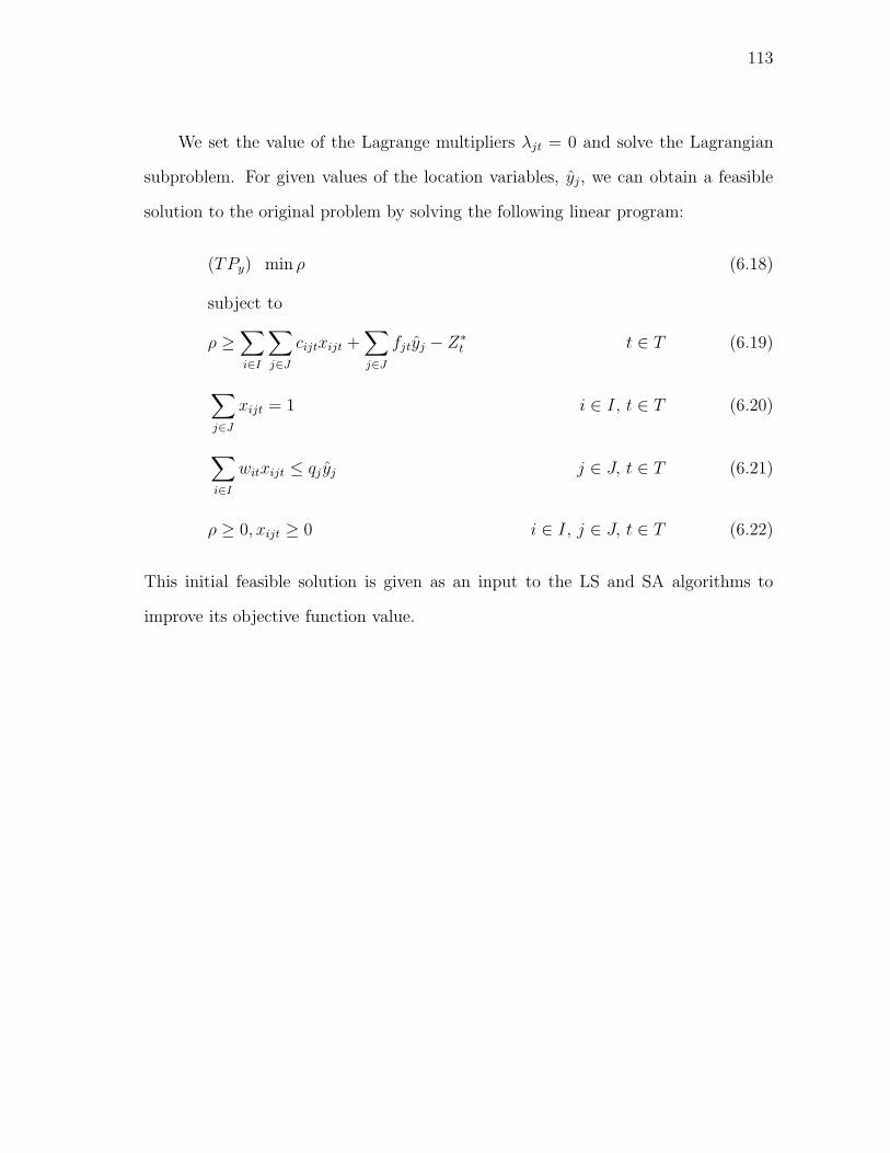
113

We set the value of the Lagrange multipliers λjt = 0 and solve the Lagrangian

subproblem. For given values of the location variables, yj, we can obtain a feasible

solution to the original problem by solving the following linear program:

(TPy) min ρ (6.18)

subject to

ρ ≥∑i∈I

∑j∈J

cijtxijt +∑j∈J

fjtyj − Z∗t t ∈ T (6.19)

∑j∈J

xijt = 1 i ∈ I, t ∈ T (6.20)

∑i∈I

witxijt ≤ qj yj j ∈ J, t ∈ T (6.21)

ρ ≥ 0, xijt ≥ 0 i ∈ I, j ∈ J, t ∈ T (6.22)

This initial feasible solution is given as an input to the LS and SA algorithms to

improve its objective function value.

114

VI.3.2. Neighborhood Function

We represent a solution by a binary vector, y, which has a value of 1 in the jth

entry if yj = 1, j ∈ J , and a value of 0 otherwise. We define the neighborhood of a

solution as the set of binary vectors with at least one different entry value. For each

feasible solution, its neighborhood is obtained by three types of moves: add, drop, and

exchange. The add move changes an entry of the binary vector y with value of 0 to 1.

The drop move changes the value of an entry from 1 to 0, provided that the resulting

set of open facilities after the move has a total capacity of at least the maximum

total demand over all periods. This ensures that closing an open facility will lead

to a feasible solution. The exchange move switches or flips the values between an

entry with value of 1 and an entry with value of 0. This move is allowed as long as

the resulting set of open facilities provides a feasible solution. Display 6 gives the

pseudo-code for the neighborhood function. We define the following notation:

O set of open facilities

O′ auxiliary set

I ′ auxiliary set

TC total cost

z binary array

q total capacity

w maximum total demand

N neighborhood

115

Display 6 Pseudo-code neighborhood function

1: Initialize: y, N = ∅, O = {j ∈ J : yj = 1}, q ←∑j∈O qj , w ← maxt∈T

{∑i∈I wit

}2: for j = 1 to m do3: if y[j] = 1 then4: if q − qj ≥ w then5: z = y6: z[j]← 07: Add z to N

8: for k = j + 1 to m do9: if y[k] = 0 then

10: if q − qj + qk ≥ w then11: z = y12: z[j]← 013: z[k]← 114: Add z to N

15: end if16: end if17: end for18: end if19: else20: z = y21: z[j]← 122: Add z to N

23: for k = j + 1 to m do24: if y[k] = 1 then25: if q + qj − qk ≥ w then26: z = y27: z[k]← 028: z[j]← 129: Add z to N

30: end if31: end if32: end for33: end if34: end for35: Return N

The binary vector y has |J | = m entries. Let � denote the number of entries of vector

y with value of 1. The total number of add moves will be equal to (m− �), the total

number of drop moves will be �, and the total number of exchange moves � (m− �).

116

Thus, the size of the entire neighborhood will be (m− �) + � + � (m− �).

The process of solving the linear program (TPy) to evaluate the objective func-

tion value for each neighborhood solution can be very time consuming when solved to

optimality. Instead, we use a heuristic algorithm to approximate the objective func-

tion value of (TPy) for each candidate solution. For each period t ∈ T , the algorithm

sorts the set I of customer locations in non-increasing order of demand wit, then

allocates the demand of each customer to the nearest open facility. If the capacity of

the facility is depleted, then the remaining demand is allocated to the second nearest

facility. The algorithm keeps track of the capacity for each open facility in each pe-

riod. The algorithm stops when all demands are allocated, then adds the associated

fixed operation costs for the open facilities.

Observe that this approach is a valid method to evaluate the objective function

value of a candidate solution, since the value obtained by solving the linear program

(TPy) differs only by the constant term Z∗t for each t ∈ T . Once the best feasible

solution is selected, its objective function value can be computed by solving problem

(TPy). Display 7 gives the pseudo-code of the approximation algorithm.

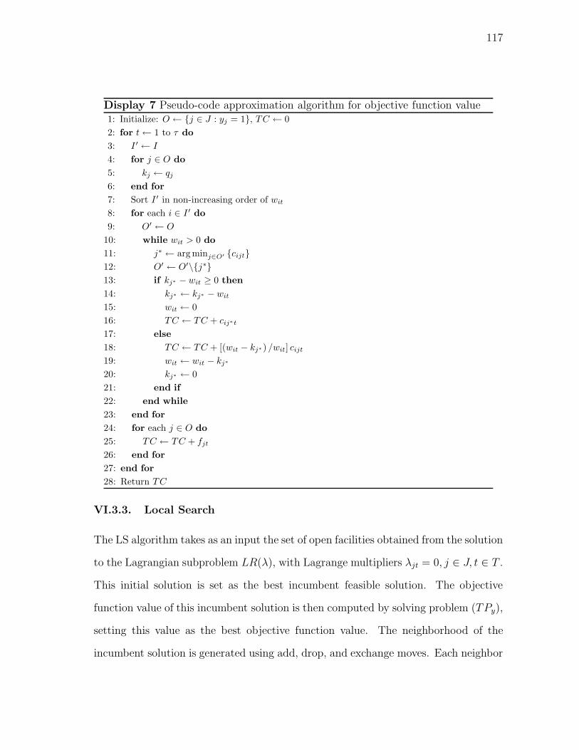
117

Display 7 Pseudo-code approximation algorithm for objective function value1: Initialize: O ← {j ∈ J : yj = 1}, TC ← 02: for t← 1 to τ do3: I ′ ← I

4: for j ∈ O do5: kj ← qj

6: end for7: Sort I ′ in non-increasing order of wit

8: for each i ∈ I ′ do9: O′ ← O

10: while wit > 0 do11: j∗ ← argminj∈O′ {cijt}12: O′ ← O′\{j∗}13: if kj∗ − wit ≥ 0 then14: kj∗ ← kj∗ − wit

15: wit ← 016: TC ← TC + cij∗t

17: else18: TC ← TC + [(wit − kj∗) /wit] cijt

19: wit ← wit − kj∗

20: kj∗ ← 021: end if22: end while23: end for24: for each j ∈ O do25: TC ← TC + fjt

26: end for27: end for28: Return TC

VI.3.3. Local Search

The LS algorithm takes as an input the set of open facilities obtained from the solution

to the Lagrangian subproblem LR(λ), with Lagrange multipliers λjt = 0, j ∈ J, t ∈ T .

This initial solution is set as the best incumbent feasible solution. The objective

function value of this incumbent solution is then computed by solving problem (TPy),

setting this value as the best objective function value. The neighborhood of the

incumbent solution is generated using add, drop, and exchange moves. Each neighbor

118

solution is evaluated using the approximation algorithm. The solution with minimum

total cost over the entire neighborhood is selected. Then, problem (TPy) is solved

again to obtain the exact objective function value. If this value is less than the

best objective function value, the new solution is taken as best incumbent feasible

solution as well as its objective function value. The process is repeated until the first

iteration when the best objective function value fails to improve. Display 8 gives the

pseudo-code for the LS algorithm. We use the following notation:

S set of open facilities

S∗ best set of open facilities

f(TPy(S)) objective function value of problem TPy given set S

Z auxiliary variable

Z∗ best objective function value

� auxiliary variable

ℵ{·} neighborhood function

N neighborhood

119

Display 8 Pseudo-code LS heuristic1: S∗ ← {j ∈ J : yj = 1}2: Solve TPy(S∗)3: Z∗ ← f (TPy(S∗))4: �← 15: while � > 0 do6: N← ℵ{S∗}7: Use approximation algorithm to find S ∈ N

8: Solve TPy(S)9: Z ← f (TPy(S))

10: if Z < Z∗ then11: Z∗ ← Z

12: S∗ = S

13: else14: �← 015: end if16: end while17: Return S∗, Z∗

VI.3.4. Simulated Annealing

The SA algorithm takes as an input the set of open facilities obtained from the

solution to the Lagrangian subproblem LR(λ), with Lagrange multipliers λjt = 0, j ∈J, t ∈ T . This initial solution is set as the best and current incumbent feasible

solution. The objective function value of this incumbent solution is then computed

by solving problem (TPy), setting this value as the best and current costs. The

algorithm calls the Metropolis subroutine giving as an input the current solution,

best solution, current cost, best cost, maximum number of iterations, and initial

temperature.

In the Metropolis subroutine, the neighborhood of the incumbent solution is

generated using add, drop, and exchange moves. A neighbor solution is randomly

selected. Then, problem (TPy) is solved again to obtain the exact objective function

value of the neighbor solution. If this solution is better than the best solution, the

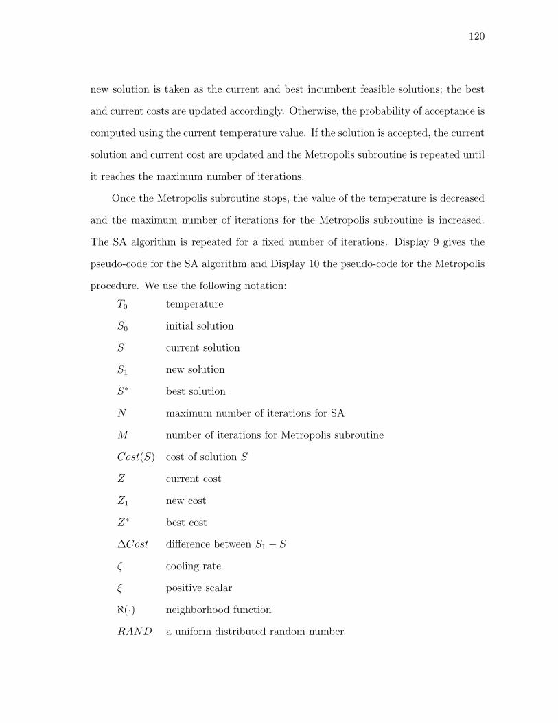
120

new solution is taken as the current and best incumbent feasible solutions; the best

and current costs are updated accordingly. Otherwise, the probability of acceptance is

computed using the current temperature value. If the solution is accepted, the current

solution and current cost are updated and the Metropolis subroutine is repeated until

it reaches the maximum number of iterations.

Once the Metropolis subroutine stops, the value of the temperature is decreased

and the maximum number of iterations for the Metropolis subroutine is increased.

The SA algorithm is repeated for a fixed number of iterations. Display 9 gives the

pseudo-code for the SA algorithm and Display 10 the pseudo-code for the Metropolis

procedure. We use the following notation:

T0 temperature

S0 initial solution

S current solution

S1 new solution

S∗ best solution

N maximum number of iterations for SA

M number of iterations for Metropolis subroutine

Cost(S) cost of solution S

Z current cost

Z1 new cost

Z∗ best cost

ΔCost difference between S1 − S

ζ cooling rate

ξ positive scalar

ℵ(·) neighborhood function

RAND a uniform distributed random number

121

e mathematical constant, e = 2.71828 . . .

Display 9 Pseudo-code SA heuristic1: Initialize: k ← 0, T0, M , N , ζ, ξ2: S ← S0

3: S∗ ← S

4: Z ← Cost(S)5: Z∗ ← Cost(S∗)6: while k < N do7: Metropolis(S,Z, S∗, Z∗, T,M)8: k ← k +M

9: T0 ← ζT0

10: M ← ξM

11: end while12: Return S∗, Z∗

Display 10 Pseudo-code Metropolis procedure1: Input: S,Z, S∗, Z∗, T0,M

2: while M > 0 do3: Randomly select S1 ∈ ℵ(S)4: Z1 ← Cost(S1)5: ΔCost← (Cost(S1)− Cost(S))6: if ΔCost < 0 then7: S ← S1

8: if Z1 < Z∗ then9: Z∗ ← Z1

10: end if11: else12: if RAND < eΔCost/T0 then13: S ← S1

14: end if15: end if16: M ←M − 117: end while18: Return S∗, Z∗

VI.4. Numerical Results

In this section we conduct a numerical experiment to test the performance of the

heuristic algorithms developed for the RCFLP.

122

We designed 12 classes of problems considering three total demand structures,

increasing, decreasing, and steady; two values for n = 50 and 100 locations; two values

for τ = 5, and 10 periods; one value of p = 0.15; and one interval to randomly generate

the fixed operation cost from a discrete uniform distribution U [100000, 150000]. The

optimal objective function value Z∗t for each period t ∈ T was computed by solving

the associated CFLP with Benders’ decomposition. Table 19 shows four classes of

problems considered in the experiments.

We solved the Lagrangian subproblem with CPLEX to optimality, setting the

value of the Lagrange multipliers λjt = 0, j ∈ J, t ∈ T . Problem (TPy) was solved

using CPLEX. We stopped the LS algorithm at the first iteration when the value of

the best feasible solution failed to improve.

For SA, we performed a test experiment to determine the values of the algorithm.

We solved 5 instances per class for each demand structure. We considered three values

for the initial temperature, T0 = 90000, 85000, and 80000. For the cooling rate, we

considered three values, ζ = 0.90, 0.88, and 0.80; three values for ξ = 1.1, 1.2, and

1.3; three values for N = 200, 300, and 500; and three values for M = 10, 15, and 20.

We selected the combination of parameter values that obtained the best minimum

regret in less computational time.

We set the initial value of the temperature T0 = 85000, the cooling rate ζ = 0.88,

scalar ξ = 1.2, the maximum number of iterations for SA N = 300, and the number of

iterations for Metropolis subroutine M = 15. The benchmark solutions were obtained

solving the RCFLP model with CPLEX, which uses a branch and cut algorithm, using

default settings and reporting the upper (UB) and lower bound (LB) values within

a maximum running time of 3600 seconds.

For each class, we solved 10 instances. For LS and SA, we reported the best

objective function value (Obj. Value) and the solution time. We computed the

123

percentage difference (Diff.) between CPLEX upper bound value and each heuristic

best objective function value, Z∗, by 100(Z∗ − UB)/UB. Tables 20 to 31 present

the computational results for each total demand structure and for each heuristic

algorithm.

From Tables 20 and 21 for increasing demand, we observe that over all classes LS

provided a lower objective function value in less computational time. In particular,

for classes 3 and 4 (with larger problem sizes) LS obtained better results. Also, LS

obtained an optimal solution for classes that were solved to optimality by CPLEX.

For decreasing demand, the results from Tables 22 and 23 show that LS obtained

an optimal solution for almost all the classes or obtained a lower objective function

value. In this case, the initial feasible solution provided a very good starting point for

the algorithm since the solution time required for all classes was smaller compared to

classes with increasing demand.

In the case of steady demand, we observe from Tables 24 and 25 that these

instances are more difficult to solve. For almost all classes CPLEX reached the maxi-

mum running time with higher average optimality gaps. Although, the improvement

in objective function value provided by LS was not as significant as in the case of

increasing and decreasing demand, it provided a good improvement in less computa-

tional time.

In general, the performance of SA was not as good as LS, but it provided a lower

objective function value for almost all the classes of problems. For increasing demand,

the computational results from Tables 26 and 27 indicate that the overall performance

of SA was better than CPLEX both in objective function value and solution time.

For decreasing demand, we observe from Tables 28 and 29 that SA obtained

optimal solutions for the same classes that CPLEX solved up to optimality. For

those instances not optimally solved, SA obtained a lower objective function value.

124

Table 19 RCFLP Classes of Problems

Parameters

Class n τ p % f

1 50 5 15 U [100000, 150000]

2 50 10 15 U [100000, 150000]

3 100 5 15 U [100000, 150000]

4 100 10 15 U [100000, 150000]

Finally, for problems with steady demand the overall performance of SA was

good, especially for some classes 1 and 3. From Tables 30 and 31 we observe that SA

provided improved objective function values compared to LS.

Over all the experiments, the performance of LS obtained better results than

SA. Note that the candidate feasible solution in LS is selected from the entire neigh-

borhood. If the initial solution reaches a region near the optimum, it is possible that

this best neighbor solution will lead to the exploration of improving solutions. In

general, the average solution time of LS is smaller since it stops whenever the best

objective function value fails to improve. On the other hand, SA randomly selects

a neighbor solution and accepts non-improving solutions with a certain probability.

This procedure allows the algorithm to leave the local optima, which is the main

limitation of LS. The average solution time for SA is larger since it runs for a fixed

number of iterations. For some classes of problems, it provided improved solutions

compared to LS.

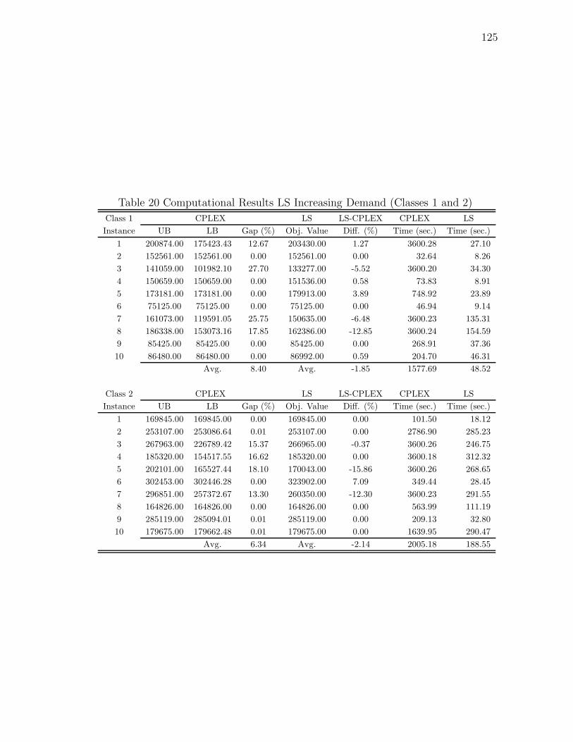
125

Table 20 Computational Results LS Increasing Demand (Classes 1 and 2)

Class 1 CPLEX LS LS-CPLEX CPLEX LSInstance UB LB Gap (%) Obj. Value Diff. (%) Time (sec.) Time (sec.)

1 200874.00 175423.43 12.67 203430.00 1.27 3600.28 27.102 152561.00 152561.00 0.00 152561.00 0.00 32.64 8.263 141059.00 101982.10 27.70 133277.00 -5.52 3600.20 34.304 150659.00 150659.00 0.00 151536.00 0.58 73.83 8.915 173181.00 173181.00 0.00 179913.00 3.89 748.92 23.896 75125.00 75125.00 0.00 75125.00 0.00 46.94 9.147 161073.00 119591.05 25.75 150635.00 -6.48 3600.23 135.318 186338.00 153073.16 17.85 162386.00 -12.85 3600.24 154.599 85425.00 85425.00 0.00 85425.00 0.00 268.91 37.3610 86480.00 86480.00 0.00 86992.00 0.59 204.70 46.31

Avg. 8.40 Avg. -1.85 1577.69 48.52

Class 2 CPLEX LS LS-CPLEX CPLEX LSInstance UB LB Gap (%) Obj. Value Diff. (%) Time (sec.) Time (sec.)

1 169845.00 169845.00 0.00 169845.00 0.00 101.50 18.122 253107.00 253086.64 0.01 253107.00 0.00 2786.90 285.233 267963.00 226789.42 15.37 266965.00 -0.37 3600.26 246.754 185320.00 154517.55 16.62 185320.00 0.00 3600.18 312.325 202101.00 165527.44 18.10 170043.00 -15.86 3600.26 268.656 302453.00 302446.28 0.00 323902.00 7.09 349.44 28.457 296851.00 257372.67 13.30 260350.00 -12.30 3600.23 291.558 164826.00 164826.00 0.00 164826.00 0.00 563.99 111.199 285119.00 285094.01 0.01 285119.00 0.00 209.13 32.8010 179675.00 179662.48 0.01 179675.00 0.00 1639.95 290.47

Avg. 6.34 Avg. -2.14 2005.18 188.55

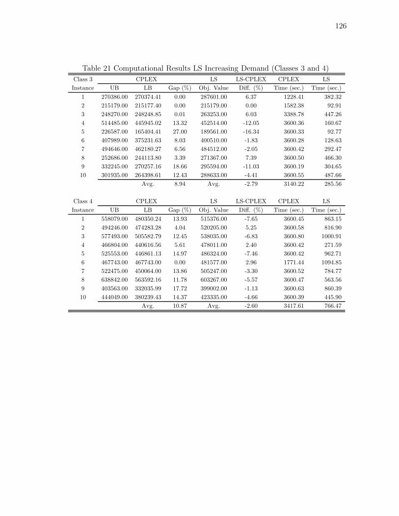
126

Table 21 Computational Results LS Increasing Demand (Classes 3 and 4)

Class 3 CPLEX LS LS-CPLEX CPLEX LSInstance UB LB Gap (%) Obj. Value Diff. (%) Time (sec.) Time (sec.)

1 270386.00 270374.41 0.00 287601.00 6.37 1228.41 382.322 215179.00 215177.40 0.00 215179.00 0.00 1582.38 92.913 248270.00 248248.85 0.01 263253.00 6.03 3388.78 447.264 514485.00 445945.02 13.32 452514.00 -12.05 3600.36 160.675 226587.00 165404.41 27.00 189561.00 -16.34 3600.33 92.776 407989.00 375231.63 8.03 400510.00 -1.83 3600.28 128.637 494646.00 462180.27 6.56 484512.00 -2.05 3600.42 292.478 252686.00 244113.80 3.39 271367.00 7.39 3600.50 466.309 332245.00 270257.16 18.66 295594.00 -11.03 3600.19 304.6510 301935.00 264398.61 12.43 288633.00 -4.41 3600.55 487.66

Avg. 8.94 Avg. -2.79 3140.22 285.56

Class 4 CPLEX LS LS-CPLEX CPLEX LSInstance UB LB Gap (%) Obj. Value Diff. (%) Time (sec.) Time (sec.)

1 558079.00 480350.24 13.93 515376.00 -7.65 3600.45 863.152 494246.00 474283.28 4.04 520205.00 5.25 3600.58 816.903 577493.00 505582.79 12.45 538035.00 -6.83 3600.80 1000.914 466804.00 440616.56 5.61 478011.00 2.40 3600.42 271.595 525553.00 446861.13 14.97 486324.00 -7.46 3600.42 962.716 467743.00 467743.00 0.00 481577.00 2.96 1771.44 1094.857 522475.00 450064.00 13.86 505247.00 -3.30 3600.52 784.778 638842.00 563592.16 11.78 603267.00 -5.57 3600.47 563.569 403563.00 332035.99 17.72 399002.00 -1.13 3600.63 860.3910 444049.00 380239.43 14.37 423335.00 -4.66 3600.39 445.90

Avg. 10.87 Avg. -2.60 3417.61 766.47

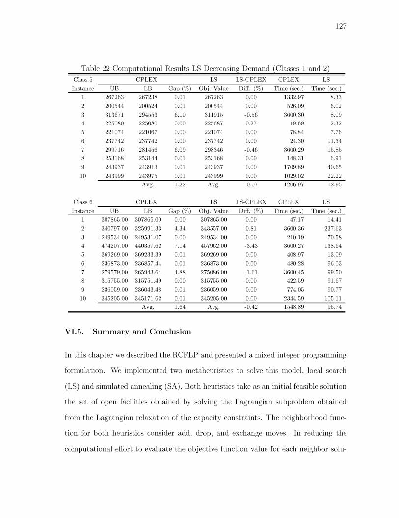
127

Table 22 Computational Results LS Decreasing Demand (Classes 1 and 2)

Class 5 CPLEX LS LS-CPLEX CPLEX LSInstance UB LB Gap (%) Obj. Value Diff. (%) Time (sec.) Time (sec.)

1 267263 267238 0.01 267263 0.00 1332.97 8.332 200544 200524 0.01 200544 0.00 526.09 6.023 313671 294553 6.10 311915 -0.56 3600.30 8.094 225080 225080 0.00 225687 0.27 19.69 2.325 221074 221067 0.00 221074 0.00 78.84 7.766 237742 237742 0.00 237742 0.00 24.30 11.347 299716 281456 6.09 298346 -0.46 3600.29 15.858 253168 253144 0.01 253168 0.00 148.31 6.919 243937 243913 0.01 243937 0.00 1709.89 40.6510 243999 243975 0.01 243999 0.00 1029.02 22.22

Avg. 1.22 Avg. -0.07 1206.97 12.95

Class 6 CPLEX LS LS-CPLEX CPLEX LSInstance UB LB Gap (%) Obj. Value Diff. (%) Time (sec.) Time (sec.)

1 307865.00 307865.00 0.00 307865.00 0.00 47.17 14.412 340797.00 325991.33 4.34 343557.00 0.81 3600.36 237.633 249534.00 249531.07 0.00 249534.00 0.00 210.19 70.584 474207.00 440357.62 7.14 457962.00 -3.43 3600.27 138.645 369269.00 369233.39 0.01 369269.00 0.00 408.97 13.096 236873.00 236857.44 0.01 236873.00 0.00 480.28 96.037 279579.00 265943.64 4.88 275086.00 -1.61 3600.45 99.508 315755.00 315751.49 0.00 315755.00 0.00 422.59 91.679 236059.00 236043.48 0.01 236059.00 0.00 774.05 90.7710 345205.00 345171.62 0.01 345205.00 0.00 2344.59 105.11

Avg. 1.64 Avg. -0.42 1548.89 95.74

VI.5. Summary and Conclusion

In this chapter we described the RCFLP and presented a mixed integer programming

formulation. We implemented two metaheuristics to solve this model, local search

(LS) and simulated annealing (SA). Both heuristics take as an initial feasible solution

the set of open facilities obtained by solving the Lagrangian subproblem obtained

from the Lagrangian relaxation of the capacity constraints. The neighborhood func-

tion for both heuristics consider add, drop, and exchange moves. In reducing the

computational effort to evaluate the objective function value for each neighbor solu-

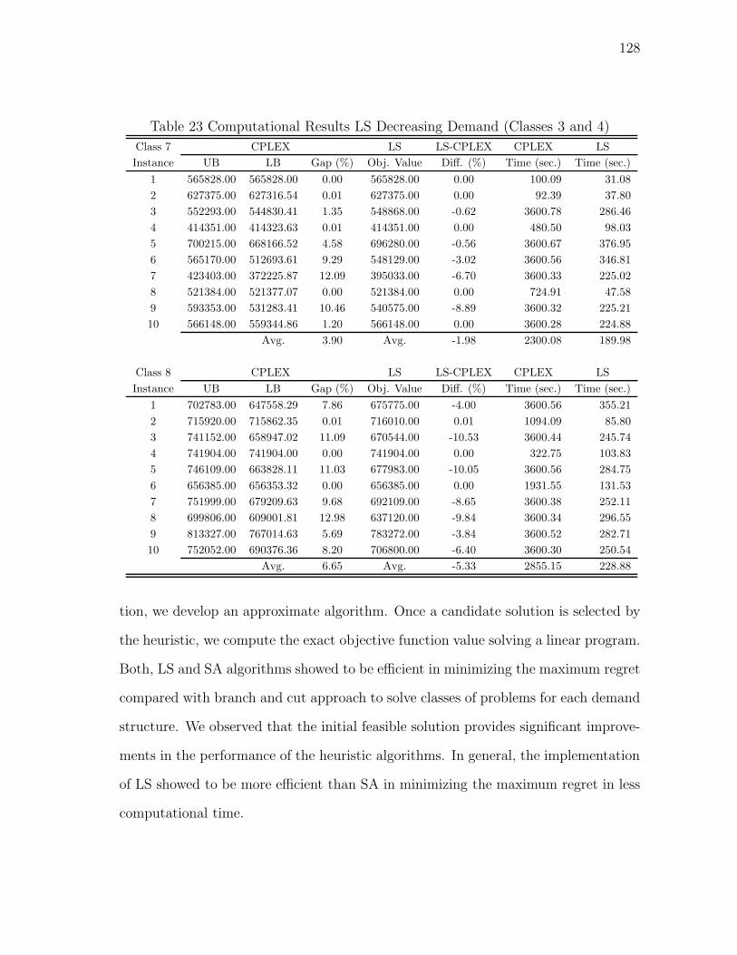
128

Table 23 Computational Results LS Decreasing Demand (Classes 3 and 4)

Class 7 CPLEX LS LS-CPLEX CPLEX LSInstance UB LB Gap (%) Obj. Value Diff. (%) Time (sec.) Time (sec.)

1 565828.00 565828.00 0.00 565828.00 0.00 100.09 31.082 627375.00 627316.54 0.01 627375.00 0.00 92.39 37.803 552293.00 544830.41 1.35 548868.00 -0.62 3600.78 286.464 414351.00 414323.63 0.01 414351.00 0.00 480.50 98.035 700215.00 668166.52 4.58 696280.00 -0.56 3600.67 376.956 565170.00 512693.61 9.29 548129.00 -3.02 3600.56 346.817 423403.00 372225.87 12.09 395033.00 -6.70 3600.33 225.028 521384.00 521377.07 0.00 521384.00 0.00 724.91 47.589 593353.00 531283.41 10.46 540575.00 -8.89 3600.32 225.2110 566148.00 559344.86 1.20 566148.00 0.00 3600.28 224.88

Avg. 3.90 Avg. -1.98 2300.08 189.98

Class 8 CPLEX LS LS-CPLEX CPLEX LSInstance UB LB Gap (%) Obj. Value Diff. (%) Time (sec.) Time (sec.)

1 702783.00 647558.29 7.86 675775.00 -4.00 3600.56 355.212 715920.00 715862.35 0.01 716010.00 0.01 1094.09 85.803 741152.00 658947.02 11.09 670544.00 -10.53 3600.44 245.744 741904.00 741904.00 0.00 741904.00 0.00 322.75 103.835 746109.00 663828.11 11.03 677983.00 -10.05 3600.56 284.756 656385.00 656353.32 0.00 656385.00 0.00 1931.55 131.537 751999.00 679209.63 9.68 692109.00 -8.65 3600.38 252.118 699806.00 609001.81 12.98 637120.00 -9.84 3600.34 296.559 813327.00 767014.63 5.69 783272.00 -3.84 3600.52 282.7110 752052.00 690376.36 8.20 706800.00 -6.40 3600.30 250.54

Avg. 6.65 Avg. -5.33 2855.15 228.88

tion, we develop an approximate algorithm. Once a candidate solution is selected by

the heuristic, we compute the exact objective function value solving a linear program.

Both, LS and SA algorithms showed to be efficient in minimizing the maximum regret

compared with branch and cut approach to solve classes of problems for each demand

structure. We observed that the initial feasible solution provides significant improve-

ments in the performance of the heuristic algorithms. In general, the implementation

of LS showed to be more efficient than SA in minimizing the maximum regret in less

computational time.

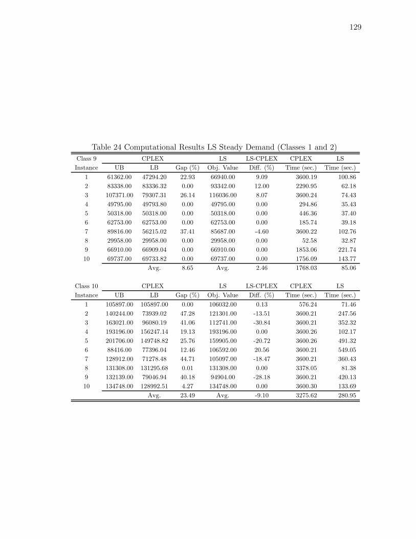
129

Table 24 Computational Results LS Steady Demand (Classes 1 and 2)

Class 9 CPLEX LS LS-CPLEX CPLEX LSInstance UB LB Gap (%) Obj. Value Diff. (%) Time (sec.) Time (sec.)

1 61362.00 47294.20 22.93 66940.00 9.09 3600.19 100.862 83338.00 83336.32 0.00 93342.00 12.00 2290.95 62.183 107371.00 79307.31 26.14 116036.00 8.07 3600.24 74.434 49795.00 49793.80 0.00 49795.00 0.00 294.86 35.435 50318.00 50318.00 0.00 50318.00 0.00 446.36 37.406 62753.00 62753.00 0.00 62753.00 0.00 185.74 39.187 89816.00 56215.02 37.41 85687.00 -4.60 3600.22 102.768 29958.00 29958.00 0.00 29958.00 0.00 52.58 32.879 66910.00 66909.04 0.00 66910.00 0.00 1853.06 221.7410 69737.00 69733.82 0.00 69737.00 0.00 1756.09 143.77

Avg. 8.65 Avg. 2.46 1768.03 85.06

Class 10 CPLEX LS LS-CPLEX CPLEX LSInstance UB LB Gap (%) Obj. Value Diff. (%) Time (sec.) Time (sec.)

1 105897.00 105897.00 0.00 106032.00 0.13 576.24 71.462 140244.00 73939.02 47.28 121301.00 -13.51 3600.21 247.563 163021.00 96080.19 41.06 112741.00 -30.84 3600.21 352.324 193196.00 156247.14 19.13 193196.00 0.00 3600.26 102.175 201706.00 149748.82 25.76 159905.00 -20.72 3600.26 491.326 88416.00 77396.04 12.46 106592.00 20.56 3600.21 549.057 128912.00 71278.48 44.71 105097.00 -18.47 3600.21 360.438 131308.00 131295.68 0.01 131308.00 0.00 3378.05 81.389 132139.00 79046.94 40.18 94904.00 -28.18 3600.21 420.1310 134748.00 128992.51 4.27 134748.00 0.00 3600.30 133.69

Avg. 23.49 Avg. -9.10 3275.62 280.95

130

Table 25 Computational Results LS Steady Demand (Classes 3 and 4)

Class 11 CPLEX LS LS-CPLEX CPLEX LSInstance UB LB Gap (%) Obj. Value Diff. (%) Time (sec.) Time (sec.)

1 118247.00 118247.00 0.00 118247.00 0.00 2706.85 113.572 120718.00 120718.00 0.00 120718.00 0.00 1729.18 312.323 113619.00 85369.13 24.86 120356.00 5.93 3600.23 788.504 94627.00 94624.20 0.00 94627.00 0.00 3179.52 112.125 176508.00 114857.37 34.93 175664.00 -0.48 3600.34 925.796 164798.00 120372.47 26.96 193083.00 17.16 3600.26 1212.767 133503.00 99524.66 25.45 132919.00 -0.44 3600.26 980.468 100485.00 93597.26 6.85 122139.00 21.55 3600.27 573.179 170397.00 99234.88 41.76 137030.00 -19.58 3600.26 729.5010 156581.00 81108.27 48.20 130918.00 -16.39 3600.35 666.04

Avg. 20.90 Avg. 0.78 3281.75 641.42

Class 12 CPLEX LS LS-CPLEX CPLEX LSInstance UB LB Gap (%) Obj. Value Diff. (%) Time (sec.) Time (sec.)

1 259174.00 203043.10 21.66 310377.00 16.50 3600.43 977.592 168000.00 149650.64 10.92 191866.00 12.44 3600.41 783.773 233450.00 163305.42 30.05 201862.00 -15.65 3600.46 1234.314 273129.00 175091.13 35.89 229240.00 -19.15 3600.73 863.185 247613.00 184005.98 25.69 218736.00 -13.20 3600.48 1044.716 297753.00 236711.97 20.50 263873.00 -12.84 3600.53 728.797 289097.00 206656.18 28.52 245165.00 -17.92 3600.45 1274.128 191863.00 126900.62 33.86 236312.00 18.81 3600.73 1236.389 303282.00 240716.07 20.63 262744.00 -15.43 3600.50 920.4010 288895.00 218745.37 24.28 276762.00 -4.38 3600.46 1285.30

Avg. 25.20 Avg. -5.08 3600.52 1034.85

131

Table 26 Computational Results SA Increasing Demand (Classes 1 and 2)

Class 1 CPLEX SA SA-CPLEX CPLEX SAInstance UB LB Gap (%) Obj. Value Diff. (%) Time (sec.) Time (sec.)

1 200874.00 175423.43 12.67 200806.00 -0.03 3600.28 129.252 152561.00 152561.00 0.00 152561.00 0.00 32.64 127.863 141059.00 101982.10 27.70 136708.00 -3.08 3600.20 141.444 150659.00 150659.00 0.00 151536.00 0.58 73.83 128.315 173181.00 173181.00 0.00 180849.00 4.43 748.92 134.396 75125.00 75125.00 0.00 75125.00 0.00 46.94 50.667 161073.00 119591.05 25.75 155529.00 -3.44 3600.23 61.338 186338.00 153073.16 17.85 162386.00 -12.85 3600.24 54.069 85425.00 85425.00 0.00 85425.00 0.00 268.91 63.3810 86480.00 86480.00 0.00 86992.00 0.59 204.70 59.60

Avg. 8.40 Avg. -1.38 1577.69 95.03

Class 2 CPLEX SA SA-CPLEX CPLEX SAInstance UB LB Gap (%) Obj. Value Diff. (%) Time (sec.) Time (sec.)

1 169845.00 169845.00 0.00 169845.00 0.00 101.50 64.422 253107.00 253086.64 0.01 253107.00 0.00 2786.90 59.113 267963.00 226789.42 15.37 270722.00 1.03 3600.26 103.924 185320.00 154517.55 16.62 185320.00 0.00 3600.18 80.385 202101.00 165527.44 18.10 170043.00 -15.86 3600.26 103.676 302453.00 302446.28 0.00 302453.00 0.00 349.44 153.287 296851.00 257372.67 13.30 303994.00 2.41 3600.23 182.098 164826.00 164826.00 0.00 164826.00 0.00 563.99 161.589 285119.00 285094.01 0.01 296871.00 4.12 209.13 145.1910 179675.00 179662.48 0.01 179675.00 0.00 1639.95 179.73

Avg. 6.34 Avg. -0.83 2005.18 123.34

132

Table 27 Computational Results SA Increasing Demand (Classes 3 and 4)

Class 3 CPLEX SA SA-CPLEX CPLEX SAInstance UB LB Gap (%) Obj. Value Diff. (%) Time (sec.) Time (sec.)

1 270386.00 270374.41 0.00 270386.00 0.00 1228.41 285.772 215179.00 215177.40 0.00 215179.00 0.00 1582.38 234.243 248270.00 248248.85 0.01 248270.00 0.00 3388.78 259.774 514485.00 445945.02 13.32 452514.00 -12.05 3600.36 224.865 226587.00 165404.41 27.00 202495.00 -10.63 3600.33 762.866 407989.00 375231.63 8.03 407889.00 -0.02 3600.28 1075.307 494646.00 462180.27 6.56 494139.00 -0.10 3600.42 443.668 252686.00 244113.80 3.39 275147.00 8.89 3600.50 242.449 332245.00 270257.16 18.66 319078.00 -3.96 3600.19 408.3910 301935.00 264398.61 12.43 291187.00 -3.56 3600.55 218.14

Avg. 8.94 Avg. -2.14 3140.22 415.54

Class 4 CPLEX SA SA-CPLEX CPLEX SAInstance UB LB Gap (%) Obj. Value Diff. (%) Time (sec.) Time (sec.)

1 558079.00 480350.24 13.93 516841.00 -7.39 3600.45 376.552 494246.00 474283.28 4.04 521168.00 5.45 3600.58 313.803 577493.00 505582.79 12.45 547825.00 -5.14 3600.80 1933.174 466804.00 440616.56 5.61 486745.00 4.27 3600.42 1275.505 525553.00 446861.13 14.97 510963.00 -2.78 3600.42 2229.256 467743.00 467743.00 0.00 467743.00 0.00 1771.44 297.057 522475.00 450064.00 13.86 509827.00 -2.42 3600.52 1108.208 638842.00 563592.16 11.78 638189.00 -0.10 3600.47 893.629 403563.00 332035.99 17.72 402420.00 -0.28 3600.63 1492.3910 444049.00 380239.43 14.37 425921.00 -4.08 3600.39 174.52

Avg. 10.87 Avg. -1.25 3417.61 1009.41

133

Table 28 Computational Results SA Decreasing Demand (Classes 1 and 2)

Class 5 CPLEX SA SA-CPLEX CPLEX SAInstance UB LB Gap (%) Obj. Value Diff. (%) Time (sec.) Time (sec.)

1 267263.00 267238.23 0.01 267263.00 0.00 1332.97 206.752 200544.00 200524.10 0.01 200544.00 0.00 526.09 205.053 313671.00 294552.69 6.10 313031.00 -0.20 3600.30 210.864 225080.00 225080.00 0.00 225687.00 0.27 19.69 205.055 221074.00 221066.82 0.00 221074.00 0.00 78.84 198.756 237742.00 237742.00 0.00 237742.00 0.00 24.30 205.807 299716.00 281456.38 6.09 298346.00 -0.46 3600.29 205.008 253168.00 253144.00 0.01 253168.00 0.00 148.31 209.009 243937.00 243912.76 0.01 243937.00 0.00 1709.89 217.4110 243999.00 243974.78 0.01 243999.00 0.00 1029.02 196.91

Avg. 1.22 Avg. -0.04 1206.97 206.06

Class 6 CPLEX SA SA-CPLEX CPLEX SAInstance UB LB Gap (%) Obj. Value Diff. (%) Time (sec.) Time (sec.)

1 307865.00 307865.00 0.00 307865.00 0.00 47.17 150.362 340797.00 325991.33 4.34 343557.00 0.81 3600.36 162.833 249534.00 249531.07 0.00 249534.00 0.00 210.19 154.954 474207.00 440357.62 7.14 457962.00 -3.43 3600.27 150.595 369269.00 369233.39 0.01 369269.00 0.00 408.97 161.926 236873.00 236857.44 0.01 236873.00 0.00 480.28 52.197 279579.00 265943.64 4.88 275086.00 -1.61 3600.45 57.868 315755.00 315751.49 0.00 315755.00 0.00 422.59 43.509 236059.00 236043.48 0.01 237190.00 0.48 774.05 47.5510 345205.00 345171.62 0.01 345205.00 0.00 2344.59 60.69

Avg. 1.64 Avg. -0.37 1548.89 104.24

134

Table 29 Computational Results SA Decreasing Demand (Classes 3 and 4)

Class 7 CPLEX SA SA-CPLEX CPLEX SAInstance UB LB Gap (%) Obj. Value Diff. (%) Time (sec.) Time (sec.)

1 565828.00 565828.00 0.00 564632.00 -0.21 100.09 100.912 627375.00 627316.54 0.01 627375.00 0.00 92.39 73.673 552293.00 544830.41 1.35 547844.00 -0.81 3600.78 119.344 414351.00 414323.63 0.01 414351.00 0.00 480.50 74.945 700215.00 668166.52 4.58 696280.00 -0.56 3600.67 107.646 565170.00 512693.61 9.29 548129.00 -3.02 3600.56 96.957 423403.00 372225.87 12.09 395033.00 -6.70 3600.33 70.508 521384.00 521377.07 0.00 521384.00 0.00 724.91 63.279 593353.00 531283.41 10.46 540575.00 -8.89 3600.32 70.8810 566148.00 559344.86 1.20 566148.00 0.00 3600.28 81.66

Avg. 3.90 Avg. -2.02 2300.08 85.97

Class 8 CPLEX SA SA-CPLEX CPLEX SAInstance UB LB Gap (%) Obj. Value Diff. (%) Time (sec.) Time (sec.)

1 702783.00 647558.29 7.86 675775.00 -4.00 3600.56 2542.262 715920.00 715862.35 0.01 716010.00 0.01 1094.09 298.143 741152.00 658947.02 11.09 670544.00 -10.53 3600.44 281.784 741904.00 741904.00 0.00 741904.00 0.00 322.75 177.015 746109.00 663828.11 11.03 677983.00 -10.05 3600.56 1599.676 656385.00 656353.32 0.00 656385.00 0.00 1931.55 160.807 751999.00 679209.63 9.68 692109.00 -8.65 3600.38 422.408 699806.00 609001.81 12.98 637120.00 -9.84 3600.34 1713.639 813327.00 767014.63 5.69 783272.00 -3.84 3600.52 1514.2610 752052.00 690376.36 8.20 706800.00 -6.40 3600.30 438.39

Avg. 6.65 Avg. -5.33 2855.15 914.83

135

Table 30 Computational Results SA Steady Demand (Classes 1 and 2)

Class 9 CPLEX SA SA-CPLEX CPLEX SAInstance UB LB Gap (%) Obj. Value Diff. (%) Time (sec.) Time (sec.)

1 61362.00 47294.20 22.93 61362.00 0.00 3600.19 83.392 83338.00 83336.32 0.00 83338.00 0.00 2290.95 48.333 107371.00 79307.31 26.14 100983.00 -5.95 3600.24 40.614 49795.00 49793.80 0.00 49795.00 0.00 294.86 46.165 50318.00 50318.00 0.00 52091.00 3.52 446.36 49.726 62753.00 62753.00 0.00 62753.00 0.00 185.74 38.447 89816.00 56215.02 37.41 91518.00 1.89 3600.22 37.198 29958.00 29958.00 0.00 29958.00 0.00 52.58 34.889 66910.00 66909.04 0.00 66910.00 0.00 1853.06 69.6610 69737.00 69733.82 0.00 69737.00 0.00 1756.09 53.94

Avg. 8.65 Avg. -0.05 1768.03 50.23

Class 10 CPLEX SA SA-CPLEX CPLEX SAInstance UB LB Gap (%) Obj. Value Diff. (%) Time (sec.) Time (sec.)

1 105897.00 105897.00 0.00 106032.00 0.13 576.24 58.252 140244.00 73939.02 47.28 121301.00 -13.51 3600.21 183.093 163021.00 96080.19 41.06 129168.00 -20.77 3600.21 125.984 193196.00 156247.14 19.13 193196.00 0.00 3600.26 86.985 201706.00 149748.82 25.76 159905.00 -20.72 3600.26 71.096 88416.00 77396.04 12.46 106032.00 19.92 3600.21 82.357 128912.00 71278.48 44.71 111228.00 -13.72 3600.21 129.728 131308.00 131295.68 0.01 131308.00 0.00 3378.05 90.639 132139.00 79046.94 40.18 94904.00 -28.18 3600.21 89.1410 134748.00 128992.51 4.27 134748.00 0.00 3600.30 75.20

Avg. 23.49 Avg. -7.68 3275.62 99.24

136

Table 31 Computational Results SA Steady Demand (Classes 3 and 4)

Class 11 CPLEX SA SA-CPLEX CPLEX SAInstance UB LB Gap (%) Obj. Value Diff. (%) Time (sec.) Time (sec.)

1 118247.00 118247.00 0.00 118247.00 0.00 2706.85 198.922 120718.00 120718.00 0.00 120718.00 0.00 1729.18 108.753 113619.00 85369.13 24.86 122607.00 7.91 3600.23 864.684 94627.00 94624.20 0.00 94627.00 0.00 3179.52 273.255 176508.00 114857.37 34.93 178339.00 1.04 3600.34 665.856 164798.00 120372.47 26.96 185660.00 12.66 3600.26 143.067 133503.00 99524.66 25.45 129498.00 -3.00 3600.26 143.808 100485.00 93597.26 6.85 122139.00 21.55 3600.27 143.639 170397.00 99234.88 41.76 170171.00 -0.13 3600.26 140.4210 156581.00 81108.27 48.20 133598.00 -14.68 3600.35 143.22

Avg. 20.90 Avg. 2.53 3281.75 282.56

Class 12 CPLEX SA SA-CPLEX CPLEX SAInstance UB LB Gap (%) Obj. Value Diff. (%) Time (sec.) Time (sec.)

1 259174.00 203043.10 21.66 312598.00 17.09 3600.43 2285.752 168000.00 149650.64 10.92 193570.00 13.21 3600.41 540.273 233450.00 163305.42 30.05 207997.00 -12.24 3600.46 730.914 273129.00 175091.13 35.89 234088.00 -16.68 3600.73 735.995 247613.00 184005.98 25.69 229582.00 -7.85 3600.48 1360.506 297753.00 236711.97 20.50 264392.00 -12.62 3600.53 1228.817 289097.00 206656.18 28.52 265622.00 -8.84 3600.45 1651.038 191863.00 126900.62 33.86 274482.00 30.10 3600.73 1972.099 303282.00 240716.07 20.63 266197.00 -13.93 3600.50 2059.4610 288895.00 218745.37 24.28 284409.00 -1.58 3600.46 2350.73

Avg. 25.20 Avg. -1.33 3600.52 1491.55

137

CHAPTER VII

CONCLUSIONS AND FUTURE DIRECTIONS

In this dissertation, we presented models for dynamic location, dynamic demand

without relocation of facilities, and robust location problems. The dynamic model

determines the optimal time and location for establishing capacitated facilities to

supply the demand of customers over a discrete and finite time horizon. The model

for dynamic demand without relocation finds a fixed configuration of capacitated

facilities to serve the time varying demand. The robust model determines a fixed

configuration of capacitated facilities with the objective of minimizing the worst-

case cost or maximum regret. This measure of robustness is commonly used in the

literature to evaluate decisions under uncertainty.

We also described three different structures for the total demand of customers

and the behavior of the demand for each customer location. These demand structures

motivate the analysis of the dynamic and robust models and provided a mean to test

the performance of the solution methods developed for each model.

The Lagrangian relaxation and Benders’ decomposition algorithms developed for

the dynamic model studied in Chapter IV performed well providing good quality solu-

tions in acceptable computational time, compared with conventional branch and cut.

The structure of the associated subproblems for each algorithm played an important

role in solving the dynamic model. We observed that for classes of problems where

the split or portion of the total average cost considers a large portion of fixed cost,

the solution algorithms have an improved performance.

The Benders’ decomposition algorithm for dynamic demand without relocation

presented in Chapter V also showed to be efficient. We showed that when relocation

138

costs are considerably large, the dynamic location model can be used to solve the

model for dynamic demand without relocation. The cost structure of the average

total cost also determined the performance of the solution algorithm as in the dynamic

model.

For the robust model studied in Chapter VI, we implemented two heuristic

algorithms, both being efficient in providing near optimal solutions in acceptable

computational time. We obtained improved solutions using a Lagrangian relaxation

approach to obtain the initial feasible solution. The neighborhood function, which

considers add, drop, and exchange moves also provided an efficient way of exploring

the neighborhood of each candidate solution. Overall the classes of problems, the

heuristic solution algorithms provided solutions with minimum worst-case regret in

less computational time than conventional branch and cut.

Future research directions for the dynamic location model is the additional re-

striction in the allocation of customers to a single facility, or single sourcing. Another

interesting area of research for the dynamic location model is to consider multi-stage

location problems, such as distribution system design. The location of facilities and

distribution centers, as well as the allocation of customers can be considered when

demand and cost parameters are time varying. The problem structure offers a pos-

sibility to implement decomposition algorithms and the analysis of different demand

structures.

For the problem of dynamic demand without relocation, we can consider a fixed

number of open facilities in each period. That is, a p-median problem with dynamic

demand and without relocation of facilities. The solution algorithms developed for

our model can be applicable to the p-median version since the only difference is that

the number of open facilities is given.

Future research for robust location model may include the consideration of dif-

139

ferent robustness measures. An interesting problem for the robust location model is

to determine the location of emergency services when demand and cost parameters

change by time and the objective is to minimize the maximum response time or min-

imizing the worst-case regret in response time. Alternative measures of robustness

can lead to a different mixed integer programming formulation for which any of the

solution algorithms developed in this dissertation may be applicable.

140

REFERENCES

Andreatta, G., F. M. Mason. 1994. A note on: A perfect forward procedure for a

single facility dynamic location/relocation problem. Operations Research Letters

15(2) 81–83.

Arostegui, M. A., S. N. Kadipasaoglu, B. M. Khumawala. 2006. An empirical com-

parison of tabu search, simulated annealing, and genetic algorithms for facilities

location problems. International Journal of Production Economics 103(2) 742–

754.

Averbakh, I. 2000. Minmax regret solutions for minimax optimization problems with

uncertainty. Operations Research Letters 27(2) 57–65.

Averbakh, I. 2005. The minmax relative regret median problem on networks. IN-

FORMS Journal on Computing 17(4) 451.

Averbakh, I., O. Berman. 1997. Minimax regret p-center location on a network with

demand uncertainty. Location Science 5(4) 247–254.

Averbakh, I., O. Berman. 2000. Algorithms for the robust 1-center problem on a tree.

European Journal of Operational Research 123(2) 292–302.

Baker, B. M., J. Sheasby. 1999. Accelerating the convergence of subgradient optimi-

sation. European Journal of Operational Research 117(1) 136–144.

Balakrishnan, J. 2004. An improved algorithm for solving a multi-period facility

location problem. IIE Transactions 36(1) 19–22.

141

Ballou, R. H. 1968. Dynamic warehouse location analysis. Journal of Marketing

Research 5(3) 271–276.

Barcelo, J., J. Casanovas. 1984. A heuristic lagrangean algorithm for the capacitated

plant location problem. European Journal of Operational Research 15(2) 212–226.

Bastian, M., M. Volkmer. 1992. A perfect forward procedure for a single facility

dynamic location/relocation problem. Operations Research Letters 12(1) 11–16.

Beasley, J. E. 1988. An algorithm for solving large capacitated warehouse location

problems. European Journal of Operational Research 33(3) 314–325.

Beasley, J. E. 1993. Lagrangean heuristics for location problems. European Journal

of Operational Research 65(3) 383–399.

Bellman, R. 1966. Dynamic programming. Science 153(3731) 34–37.

Benders, J. F. 1962. Partitioning procedures for solving mixed-variables programming

problems. Numerische Mathematik 4(1) 238–252.

Brandeau, M. L., S. S. Chiu. 1989. An overview of representative problems in location

research. Management Science 35(6) 645–674.

Canel, C., S. R. Das. 1999. The uncapacitated multi-period facilities location problem

with profit maximization. International Journal of Physical Distribution & Logistics

Management 29(6) 409–433.

Canel, C., B. M. Khumawala. 1996. A mixed-integer programming approach for the

international facilities location problem. International Journal of Operations &

Production Management 16(4) 49–68.

142

Canel, C., B. M. Khumawala. 1997. Multi-period international facilities location:

an algorithm and application. International Journal of Production Research 35(7)

1891–1910.

Carrizosa, E., S. Nickel. 2003. Robust facility location. Mathematical Methods of

Operations Research (ZOR) 58(2) 331–349.

Chand, S. 1988. Decision/forecast horizon results for a single facility dynamic loca-

tion/relocation problem. Operations Research Letters 7(5) 247–251.

Chardaire, P., A. Sutter, M. C. Costa. 1996. Solving the dynamic facility location

problem. Networks 28(2) 117–124.

Chrissis, J. W., R. P. Davis, D. M. Miller. 1982. Dynamic set covering problem.

Applied Mathematical Modelling 6(1) 2–6.

Christofides, N., J. E. Beasley. 1983. Extensions to a lagrangean relaxation approach

for the capacitated warehouse location problem. European Journal of Operational

Research 12(1) 19–28.

Cornuejols, G., M. L. Fisher, G. L. Nemhauser. 1977. Location of bank accounts to

optimize float: An analytic study of exact and approximate algorithms. Manage-

ment Science 23(8) 789–810.

Cornuejols, G., R. Sridharan, J. M. Thizy. 1991. A comparison of heuristics and relax-

ations for the capacitated plant location problem. European Journal of Operational

Research 50(3) 280–297.

Current, J., S. Ratick, C. ReVelle. 1998. Dynamic facility location when the total

number of facilities is uncertain: A decision analysis approach. European Journal

of Operational Research 110(3) 597–609.

143

Daskin, M. S. 1995. Network and Discrete Location: Models Algorithms and Appli-

cations . Wiley, New York, NY, USA.

Daskin, M. S., S. M. Hesse, C. S. Revelle. 1997. α-Reliable p-minimax regret: A new

model for strategic facility location modeling. Location Science 5(4) 227–246.

Daskin, M. S., W. J. Hopp, B. Medina. 1992. Forecast horizons and dynamic facility

location planning. Annals of Operations Research 40(1) 125–151.

Dias, J., M. E. Captivo, J. Clımaco. 2001a. Capacitated dynamic location problems

with opening, closure and reopening of facilities. Research report, INESC-Coimbra,

Lisboa, Portugal.

Dias, J., M. E. Captivo, J. Clımaco. 2001b. A hybrid algorithm for dynamic location

problems. Research report, INESC-Coimbra, Lisboa, Portugal.

Dias, J., M. E. Captivo, J. Clımaco. 2004a. Dynamic location problems with discrete

expansion and reduction sizes of available capacities. Research report, INESC-

Coimbra, Lisboa, Portugal.

Dias, J., M. E. Captivo, J. Clımaco. 2004b. Dynamic multi-level capacitated and un-

capacitated location problems: An approach using primal-dual heuristics. Research

report, INESC-Coimbra, Lisboa, Portugal.

Drezner, T., Z. Drezner, S. Salhi. 2002. Solving the multiple competitive facilities

location problem. European Journal of Operational Research 142(1) 138–151.

Drezner, Z. 1984. The planar two-center and two-median problems. Transportation

Science 18 351–361.

Drezner, Z. 1995a. Dynamic facility location: The progressive p-median problem.

Location Science 3(1) 1–7.

144

Drezner, Z. 1995b. Facility location: A Survey of Applications and Methods. Springer-

Verlag, New York, NY, USA.

Drezner, Z., H. Hamacher. 2002. Facility Location: Applications and Theory .

Springer-Verlag, New York, NY, USA.

Drezner, Z., G. O. Wesolowsky. 1991. Facility location when demand is time depen-

dent. Naval Research Logistics 38(5) 763–777.

Efroymson, M. A., T. L. Ray. 1966. A branch-bound algorithm for plant location.

Operations Research 14(3) 361–368.

Erlenkotter, D. 1974. Dynamic facility location and simple network models. Manage-

ment Science 20(9) 1311–1311.

Erlenkotter, D. 1978. A dual-based procedure for uncapacitated facility location.

Operations Research 26(6) 992–1009.

Erlenkotter, D. 1981. A comparative study of approaches to dynamic location prob-

lems. European Journal of Operational Research 6 133–143.

Fisher, M. L. 2004. The lagrangian relaxation method for solving integer programming

problems. Management Science 50(13) 1861–1871.

Francis, R. L., P. B. Mirchandani. 1990. Discrete location theory . Wiley, New York,

NY, USA.

Frantzeskakis, M., C. D. T. Watson-Gandy. 1989. The use of state space relaxation

for the dynamic facility location problem. Annals of Operations Research 18(1)

187–211.

145

Geoffrion, A. M. 1974. Lagrangean relaxation for integer programming. Mathematical

Programming Study 2(1974) 82–114.

Geoffrion, A. M., G. W. Graves. 1974. Multicommodity distribution system design

by benders decomposition. Management Science 20(5) 822–844.

Geoffrion, A. M., R. McBride. 1978. Lagrangean relaxation applied to capacitated

facility location problems. IIE Transactions 10(1) 40–47.

Guignard-Spielberg, M., K. Spielberg. 1977. A dual method for the mixed plant loca-

tion problem. Department of Statistics, University of Pennsylvania, The Wharton

School, Philadelphia, PA, USA.

Gunawardane, G. 1982. Dynamic versions of set covering type public facility location

problems. European Journal of Operational Research 10(2) 190–195.

Hakimi, S. L., M. Labbe, E. F. Schmeichel. 1999. Locations on time-varying networks.

Networks 34(4) 250–257.

Held, M., R. M. Karp. 1970. The traveling salesman problem and minimum spanning

trees. Operations Research 18(6) 1138–1162.

Held, M., R. M. Karp. 1971. The traveling-salesman problem and minimum spanning

trees: Part ii. Mathematical Programming 1(1) 6–25.

Held, M., P. Wolfe, H. P. Crowder. 1974. Validation of subgradient optimization.

Mathematical Programming 6(1) 62–88.

Hindi, K. S., K. Pienkosz. 1999. Efficient solution of large scale, single-source, capac-

itated plant location problems. Journal of the Operational Research Society 50(3)

268–274.

146

Holmberg, K., M. Ronnqvist, D. Yuan. 1999. An exact algorithm for the capacitated

facility location problems with single sourcing. European Journal of Operational

Research 113(3) 544–559.

Hormozi, A. M., B. M. Khumawala. 1996. An improved algorithm for solving a

multi-period facility location problem. IIE Transactions 28(2) 105–114.

Kelly, D. L., A. J. Marucheck. 1984. Planning horizon results for the dynamic ware-

house location problem. Journal of Operations Management 4 279–94.

Khumawala, B. M. 1972. An efficient branch-bound algorithm for the warehouse

location problem. Management Science 18(12) 718–732.

Kilmer, R. L., T. Spreen, D. S. Tilley. 1983. A dynamic plant location model: The east

florida fresh citrus packing industry. American Journal of Agricultural Economics

65(4) 730–737.

Kincaid, R. K. 1992. Good solutions to discrete noxious location problems via meta-

heuristics. Annals of Operations Research 40(1) 265–281.

Kirkpatrick, S., C. D. Gelatt, M. P. Vecchi. 1983. Optimization by simulated anneal-

ing. Science 220(4598) 671–680.

Klincewicz, J. G., H. Luss. 1986. Lagrangian relaxation heuristic for capacitated

facility location with single-source constraints. Journal of the Operational Research

Society 37 495–500.

Kolesar, P., W. E. Walker. 1974. An algorithm for the dynamic relocation of fire

companies. Operations Research 22(2) 249–274.

Kouvelis, P., G. Yu. 1997. Robust Discrete Optimization and Its Applications.

Springer, Secaucus, NJ, USA.

147

Kuehn, A. A., M. J. Hamburger. 1963. A heuristic program for locating warehouses.

Management Science 9(4) 643–666.

Love, R. F., J. G. Morris, G. O. Wesolowsky. 1988. Facilities Location: Models &

Methods. North-Holland, New York, NY, USA.

Magnanti, T. L., R. T. Wong. 1981. Accelerating Benders decomposition: Algorithmic

enhancement and model selection criteria. Operations Research 29(3) 464–484.

Manne, A. S. 1967. Investments for Capacity Expansion: Size, Location and Time

Phasing . The MIT Press, Cambridge, MA, USA.

Mavridou, T. D., P. M. Pardalos. 1997. Simulated annealing and genetic algorithms

for the facility layout problem: A survey. Computational Optimization and Appli-

cations 7(1) 111–126.

McDaniel, D., M. Devine. 1977. A modified Benders partitioning algorithm for mixed

integer programming. Management Science 24(3) 312–319.

Megiddo, N. 1986. Dynamic location problems. Annals of Operations Research 6(10)

311–319.

Nauss, R. M. 1978. An improved algorithm for the capacitated facility location

problem. Journal of the Operational Research Society 29(12) 1195–1201.

Nemhauser, G. L., L. A. Wolsey. 1988. Integer and Combinational Optimization.

John Wiley & Sons, New York, NY, USA.

Owen, H. S., M. S. Daskin. 1998. Strategic facility location: A review. European

Journal of Operational Research 111(3) 423–447.

148

Revelle, C., C. Toregas, L. Falkson. 1976. Applications of the location set-covering

problem. Geographical Analysis 8 65–76.

Rıos-Ramırez, A. 2003. International assembly facility location problem. Investigacion

Multidisciplinaria 1(1) 1–8.

Roodman, G. M., L. B. Schwarz. 1975. Optimal and heuristic facility phase-out

strategies. AIIE Transactions 7(2) 177–184.

Roodman, G. M., L. B. Schwarz. 1977. Extensions of the multi-period facility phase-

out model: New procedures and applications to a phase-in/phase-out problem.

AIIE Transactions 9(1) 103–107.

Saldanha da Gama, F., M. E. Captivo. 1998. A heuristic approach for the discrete

dynamic location problem. Location Science 6(1) 211–223.

Schilling, D. 1980. Dynamic location modeling for public-sector facilities: A multi-

criteria approach. Decision Sciences 11(4) 714–724.

Scott, A. J. 1971. Dynamic location-allocation systems: Some basic planning strate-

gies. Environment and Planning A 3(1) 73–82.

Serra, D., V. Marianov. 1998. The p-median problem in a changing network: The

case of Barcelona. Location Science 6(1-4) 383–394.

Shulman, A. 1991. An algorithm for solving capacitated plant location problems with

discrete expansion sizes. Operations Research 39(3) 423–36.

Snyder, L., M. Daskin. 2006. Stochastic p-robust location problems. IIE Transactions

38(11) 971–985.

149

Snyder, L. V. 2006. Facility location under uncertainty: A review. IIE Transactions

38(7) 547–564.

Sridharan, R. 1993. A lagrangian heuristic for the capacitated plant location problem

with single source constraints. European Journal of Operational Research 66(3)

305–312.

Sweeney, D. J., R. L. Tatham. 1976. An improved long-run model for multiple ware-

house location. Management Science 22(7) 748–758.

Vairaktarakis, G. L., P. Kouvelis. 1999. Incorporation dynamic aspects and uncer-

tainty in 1-median location problems. Naval Research Logistics 46(2) 147–168.

van Laarhoven, P. J. M., E. H. L. Aarts. 1987. Simulated Annealing: Theory and

Applications. Reidel, Dordrecht, The Netherlands.

Van Roy, T. J. 1986. A cross decomposition algorithm for capacitated facility location.

Operations Research 34(1) 145–163.

Van Roy, T. J., D. Erlenkotter. 1982. A dual based procedure for dynamic facility

location. Management Science 28 1091–1105.

Weber, A., C. J. Friedrich. 1929. Alfred Weber’s Theory of the Location of Industries.

The University of Chicago Press, Chicago, IL, USA.

Wentges, P. 1996. Accelerating Benders’ decomposition for the capacitated facility

location problem. Mathematical Methods of Operations Research 44(2) 267–290.

Wesolowsky, G. O. 1973. Dynamic facility location. Management Science 19(11)

1241–1248.

150

Wesolowsky, G. O., W. G. Truscott. 1975. The multiperiod location-allocation prob-

lem with relocation of facilities. Management Science 22(1) 57–65.

Wesolowsky, G. O., W. G. Truscott. 1976. Dynamic location of multiple facilities

for a class of continuous problems. American Institute of Industrial Engineers

Transactions 8(1) 76–83.

151

VITA

Joaquin Emmanuel Torres Soto received his Bachelor of Science degree in Indus-

trial and Systems Engineering in 2001 and his Master of Engineering degree in Quality

Systems and Productivity in 2003, both from Tecnologico de Monterrey Campus Chi-

huahua. He worked for three years as a research assistant, lecturer, and coordinator

of the Research Department of the School of Business and Humanities at Tecnologico

de Monterrey Campus Chihuahua. He received a scholarship from CONACYT (Con-

sejo Nacional de Ciencia y Tecnologıa) in 2004 and joined the Industrial and Systems

Engineering Department at Texas A&M University for doctoral studies. After re-

ceiving his Ph.D. he joined the faculty of Tecnologico de Monterrey. His research

interest areas are discrete optimization, facility location, and logistics systems design.

He is currently working on a joint research project with CONACYT and Tecnologico

de Monterrey related to facility location in the public sector. Mr. Torres Soto may

be reached at Tecnologico de Monterrey Campus Chihuahua, 4700 H. Colegio Mil-

itar, Col. Nombre de Dios, Chihuahua, Chih., Mexico 31050. His email address is

joaquin.torres@itesm.mx.