social network analysis for business process discovery · resumo ap erspectiva organizacional da...

Social Network Analysisfor Business Process Discovery

Claudia Sofia da Costa Alves

Dissertation for the degree of Master inInformation Systems and Computer Engineering

Supervisor: Prof. Doutor Diogo R. Ferreira

President: Prof. Alberto Manuel Rodrigues da SilvaVogal: Prof. Miguel Leitao Bignolas Mira da Silva

July 2010

placeholder

Acknowledgments

To my family, especially my parents, who have always supported me during my aca-demic carrier.

To Prof. Diogo Ferreira for his excellent assistance and availability to help. The sup-port and guidance I received throughout this year greatly improved the value of thisdissertation.

To Alvaro Rebuge ,a member of our research group, for the exchange of ideas and knowl-edge that were really helpful for the development of the case study.

Last but not the least, to all my close friends, colleagues and all the others that markedmy life course during or before this master degree a special compliment is due.

iii

placeholder

Abstract

The organizational perspective of Process Mining is a valuable technique that al-lows discovering the social network of an organization. By doing so, provides

means to evaluate networks by mapping and analyzing relationships among people,teams, departments or even entire organizations. However, when analyzing networksof large size, Process Mining techniques generate highly complex models, usually called”spaghetti models”, that may be confusing and difficult to understand.

In this dissertation we present an approach that aims to overcome this difficulty by pre-senting the information in a way that can be easily read by users. Clustering techniquesadopting a divide-and-conquer strategy are applied for this purpose as they make pos-sible the user to visualize and analyze the network in different levels of abstraction. Ourapproach also makes use of the concept of Modularity, indicating which iteration of theclustering algorithm best represents different user groups in the social network.

This approach was implemented in the ProM framework and all the experiments wereperformed in that environment. Taking into consideration the results achieved for a real-world case study and the results of several experiments, we reached the conclusion thatthe approach is capable of dealing with complex logs and that the Modularity conceptprovides a good hint of which group of clusters best represents the user groups in asocial network.

Keywords: Process Mining , Social Network Analysis , ProM Framework , Cluster-ing , Agglomerative Hierarchical Clustering , Organizational Modelling , Communities, Modularity

v

placeholder

Resumo

Ap erspectiva organizacional da extraccao de processos e uma tecnica importante quepermite descobrir a rede social de uma organizacao. Esta tecnica fornece meios

para avaliar redes sociais atraves do mapeamento e da analise das relacoes existentesentre pessoas, equipas, departamentos ou ate mesmo organizacoes inteiras. No entanto,quando se procede a analise de redes sociais de grandes dimensoes, as tecnicas actuaisgeram modelos muito complexos. Com o objectivo de superar esta dificuldade, apre-sentamos neste trabalho uma abordagem capaz de representar grandes quantidades deinformacao de forma simples e de modo a facilitar a analise e a compreensao dos dados.As tecnicas de clustering podem ser usadas para este proposito uma vez que permitemanalisar a informacao da rede a diferentes nıveis de abstraccao. A nossa abordagemadopta um algoritmo de Clustering Hierarquico Aglomerativo. O conceito de Modular-idade foi tambem adoptado com o objectivo de determinar qual a iteracao do algoritmoque melhor representa as comunidades existentes na rede. A abordagem foi implemen-tada na ferramenta ProM. Para demonstrar a sua aplicacao foi realizado um caso de es-tudo real, e tendo em consideracao os resultados obtidos concluımos que a abordagem ecapaz de lidar com logs complexos e que o conceito de modularidade realmente forneceum ideia de qual o grupo de comunidades que melhor representa os grupos sociais darede.

Palavras-Chave: Extraccao de processos , Analise de Redes Socias , Ferramenta ProM ,Clustering , Clustering Aglomerativo Hierarquico , Modelacao Organizacional , Comu-nidades , Modularidade

vii

placeholder

Contents

Acknowledgments iii

Abstract v

Resumo vii

1 Introduction 2

1.1 Process Mining . . . . . . . . . . . . . . . . . . . . . . . . . . . . . . . . . . 2

1.2 Motivation . . . . . . . . . . . . . . . . . . . . . . . . . . . . . . . . . . . . . 4

1.3 Document Structure . . . . . . . . . . . . . . . . . . . . . . . . . . . . . . . 5

2 Mining the Organizational Perspective 7

2.1 Deriving social networks from event logs . . . . . . . . . . . . . . . . . . . 7

2.2 Techniques for Social Network Mining . . . . . . . . . . . . . . . . . . . . . 9

2.2.1 Social Network Miner . . . . . . . . . . . . . . . . . . . . . . . . . . 10

2.2.2 Organizational Miner . . . . . . . . . . . . . . . . . . . . . . . . . . 11

2.2.3 Role Hierarchy Miner . . . . . . . . . . . . . . . . . . . . . . . . . . 11

2.2.4 Semantic Organizational Miner . . . . . . . . . . . . . . . . . . . . . 13

2.2.5 Staff Assignment Miner . . . . . . . . . . . . . . . . . . . . . . . . . 13

2.3 The ProM Framework . . . . . . . . . . . . . . . . . . . . . . . . . . . . . . 13

2.4 Conclusion . . . . . . . . . . . . . . . . . . . . . . . . . . . . . . . . . . . . . 15

3 Social Network Analysis 17

3.1 Social Network Analysis (SNA) . . . . . . . . . . . . . . . . . . . . . . . . . 17

3.2 SNA Measures . . . . . . . . . . . . . . . . . . . . . . . . . . . . . . . . . . . 18

3.2.1 Measures for an individual level. . . . . . . . . . . . . . . . . . . . 18

3.2.2 Measures for the network level . . . . . . . . . . . . . . . . . . . . . 19

3.3 Finding community structures in networks . . . . . . . . . . . . . . . . . . 20

ix

3.3.1 Traditional Approaches . . . . . . . . . . . . . . . . . . . . . . . . . 21

3.3.2 Recent Approaches . . . . . . . . . . . . . . . . . . . . . . . . . . . . 23

3.4 Conclusion . . . . . . . . . . . . . . . . . . . . . . . . . . . . . . . . . . . . . 24

4 Proposed Approach 27

4.1 Motivation . . . . . . . . . . . . . . . . . . . . . . . . . . . . . . . . . . . . . 27

4.2 Proposal . . . . . . . . . . . . . . . . . . . . . . . . . . . . . . . . . . . . . . 28

4.2.1 Application of Agglomerative Hierarchical Clustering in SNA . . . 29

4.2.2 Displaying social networks . . . . . . . . . . . . . . . . . . . . . . . 32

4.3 Conclusion . . . . . . . . . . . . . . . . . . . . . . . . . . . . . . . . . . . . . 34

5 Implementation in ProM 37

5.1 Extracting information from Log file . . . . . . . . . . . . . . . . . . . . . . 37

5.2 Agglomerative Hierarchical Clustering . . . . . . . . . . . . . . . . . . . . 40

5.3 Modularity . . . . . . . . . . . . . . . . . . . . . . . . . . . . . . . . . . . . . 43

5.3.1 Definition of Modularity . . . . . . . . . . . . . . . . . . . . . . . . . 43

5.4 Working Together vs. Similar Tasks . . . . . . . . . . . . . . . . . . . . . . . 46

5.5 Conclusion . . . . . . . . . . . . . . . . . . . . . . . . . . . . . . . . . . . . . 49

6 Case Study 51

6.1 Similar Tasks . . . . . . . . . . . . . . . . . . . . . . . . . . . . . . . . . . . . 53

6.2 Working Together . . . . . . . . . . . . . . . . . . . . . . . . . . . . . . . . . 54

6.2.1 First Approach - ”‘Who works with whom?”’ . . . . . . . . . . . . 54

6.2.2 Second Approach - ”‘Which specialties work together?”’ . . . . . . 56

6.3 Relationship to the Business Process . . . . . . . . . . . . . . . . . . . . . . 62

6.4 Conclusion . . . . . . . . . . . . . . . . . . . . . . . . . . . . . . . . . . . . . 63

7 Conclusions 67

7.1 Main Contributions . . . . . . . . . . . . . . . . . . . . . . . . . . . . . . . . 67

7.2 Future work . . . . . . . . . . . . . . . . . . . . . . . . . . . . . . . . . . . . 68

Bibliography 70

A Log File - insuranceClaimHandlingExample.mxml 74

B User Manual for the Social Network Mining Plug-in 81

x

placeholder

List of Tables

2.1 Table representing the content of a fragment from an event log . . . . . . . 8

5.2 Table representing the information in insuranceClaimHandlingExample.mxmlevent log. . . . . . . . . . . . . . . . . . . . . . . . . . . . . . . . . . . . . . . 39

5.3 Information extracted from the Log file (insuranceClaimHandlingExam-ple.mxml). This matrix shows the existing links among vertices. . . . . . . 40

5.4 Adjacency matrix, of insuranceClaimHandlingExample.mxml used to com-pute modularity. . . . . . . . . . . . . . . . . . . . . . . . . . . . . . . . . . . 44

5.5 Originators’ Degree of insuranceClaimHandlingExample.mxml social net-work. . . . . . . . . . . . . . . . . . . . . . . . . . . . . . . . . . . . . . . . . 45

5.6 This table shows how many times each originator performs each task. . . 47

5.7 This table shows how many tasks two originators perform in common. . . 49

6.8 Characteristics of the three Hospital Log Files. . . . . . . . . . . . . . . . . 52

xii

placeholder

List of Figures

1.1 Business Process Management life cycle showing the three phases whereprocess mining is focused (dark blue circles) . . . . . . . . . . . . . . . . . 3

2.2 Doing Similar Tasks as displayed in ProM 5.2. . . . . . . . . . . . . . . . . 10

2.3 Hierarchical clustering result represented as a dendogram (Snapshot fromProM v5.2). . . . . . . . . . . . . . . . . . . . . . . . . . . . . . . . . . . . . . 12

2.4 Organization model derived from the dendogram. Ovals and the pen-tagons represent actors/originators and organizational entities respectively.(Snapshot from ProM v5.2) . . . . . . . . . . . . . . . . . . . . . . . . . . . . 12

2.5 Overview of the ProM Framework (adapted from [27]) . . . . . . . . . . . 14

2.6 MXML format (adapted from [8]) . . . . . . . . . . . . . . . . . . . . . . . . 15

2.7 MXML snapshot . . . . . . . . . . . . . . . . . . . . . . . . . . . . . . . . . . 16

3.8 Network with community structure. In this case there are three commu-nities (represented by the dashed circles) composed by densely connectedvertices. Links of lower density (depicted with thinner lines) are the onesthat establish a connection between the different communities . . . . . . . 21

4.9 Comparison of the different phases supported by the ProM and other soft-war packages during a social network analysis . . . . . . . . . . . . . . . . 28

4.10 Output of Prom 5.2 using the Working Together mining tool applied on asmall network. In this case we used DecisionMinerLog.xml supplied byProM 5.2 . . . . . . . . . . . . . . . . . . . . . . . . . . . . . . . . . . . . . . 31

4.11 Output of Prom 5.2 using the Working Together mining tool applied on alarge network. In this case we used outpatientClinicExample.mxml sup-plied by ProM 5.2. It is relevant to say that the mining result image is justa tiny part of the real network. . . . . . . . . . . . . . . . . . . . . . . . . . 32

4.12 Social Network of the insuranceClaimHandlingExample.mxml. This screen-shot corresponds to the 1st iteration of Working Together AHC Algorithm,using tie break with modularity. At this point each cluster corresponds toa single originator. . . . . . . . . . . . . . . . . . . . . . . . . . . . . . . . . 33

4.13 Matrix showing the relationships among originators of the social networkdepicted in Figure 4.12 . . . . . . . . . . . . . . . . . . . . . . . . . . . . . . 34

xiv

1

5.14 Social Network of the insuranceClaimHandlingExample.mxml. This screen-shot corresponds to the 3rd iteration of Working Together AHC Algo-rithm, using tie break with modularity. Here the relationships amongoriginators of the social network are represented. Originators from thesame cluster are represented by the same colour. . . . . . . . . . . . . . . . 41

5.15 Social Network of the insuranceClaimHandlingExample.mxml. This screen-shot represents the organization units at the 3rd iteration of Working To-gether AHC Algorithm, using tie break with modularity . . . . . . . . . . 42

5.16 Modularity Chart. . . . . . . . . . . . . . . . . . . . . . . . . . . . . . . . . . 47

5.17 Similar Tasks Algorithm - Social Perspective . . . . . . . . . . . . . . . . . 48

5.18 Similar Tasks Algorithm - Organizational Perspective . . . . . . . . . . . . 48

6.19 Similar Tasks - Modularity Best Case. . . . . . . . . . . . . . . . . . . . . . 54

6.20 Similar Tasks - Modularity Worst Case. . . . . . . . . . . . . . . . . . . . . 55

6.21 Social network of the event log with 12 days. This is the output of theiteration with the highest modularity of Average Linkage with tie break. . 57

6.22 Matrix from log 12 days showing relationships among nurses . . . . . . . 58

6.23 Social network of the event log with 12 days. This is the output of theiteration with the highest modularity of Complete Linkage with tie break.GREEN = Emergency, BLUE = Pediatrics; PINK = Obstetrics/Gynecol-ogy, RED = Orthopedics, ORANGE = Emergency relay, DARK PURPLE= General surgery, LIGHT PURPLE = Neurology and BROWN = InternalMedicine . . . . . . . . . . . . . . . . . . . . . . . . . . . . . . . . . . . . . . 59

6.24 Social network of the event log with 14 days. This is the output of theiteration with the highest modularity of Single Linkage. . . . . . . . . . . . 61

6.25 Social network of the event log with 14 days. This is the output of theiteration with the highest modularity of Complete Linkage. . . . . . . . . . 61

6.26 Emergency Department Business Process . . . . . . . . . . . . . . . . . . . 63

7.27 Matrix view of the sub-network from Organization Unit 0 from iterationwith the highest modularity of Average Linkage with tie break from 12days event log. . . . . . . . . . . . . . . . . . . . . . . . . . . . . . . . . . . . 68

7.28 Graph view of the sub-network from Organization Unit 0 from iterationwith the highest modularity of Average Linkage with tie break from 12days event log. . . . . . . . . . . . . . . . . . . . . . . . . . . . . . . . . . . . 69

Chapter 1

Introduction

Nowadays we live in a very competitive market, where customer’s needs and expec-tations are always changing. Industry requirements are also changing and many

mergers and acquisitions are taking place. All these permanent changes are a challengefor organizations. To gain a competitive advantage, organizations must revise, changeand improve their strategic business processes, in a fast and efficient way, in order not tolose market share.

To optimize a business process, organizations must understand how the process is beingperformed, which usually involves a long period of analysis, including interviews withall the persons responsible for a given part of the process.

The use and proliferation of Process-Aware Information Systems cite2 (such as ERP,WfM, CRM and SCM systems) has led the way to a more efficient type of method tostudy the execution of processes, called process mining [17]. These systems typicallyrecord events carried out during a business process execution on event logs and theanalysis of those logs can yield important knowledge to improve quality of the organi-zation’s services and processes. Here is where process mining comes in.

In next Sections we will explain how Process Mining concept appeared and what it itspurpose.

1.1 Process Mining

Business Process Management (BPM) systems are an effort to help organizations man-aging process changes that are required in many areas of the business [3]. These systemshave been widely used and are the best methodology so far. Ideally, they should pro-vide support for the complete BPM life-cycle (Fig. 1.1): (re)design, modelling, execution,monitoring, and analysis of processes. However, existing BPM tools are unable to sup-port the full life-cycle. These tools provide strong support in design, configuration andexecution phases. Nevertheless, process monitoring, analysis and redesign phases re-ceive limited support[18]. One reason to say this lays in the fact that the analysis phaseis focused in processes performance, being the major goal identifying their weaknesses.Unfortunately, this phase is limited to simple performance indicators, such as flow time.

2

1.1. PROCESS MINING 3

Figure 1.1: Business Process Management life cycle showing the three phases where processmining is focused (dark blue circles)

For a further analysis, i.e., identifying structures or patterns in processes and organiza-tions, BPM systems require human intervention because these systems are not able tohighlight weaknesses automatically, much less suggest improvements[18]. Therefore,the re-design phase is affected, because has no information to be able to suggest alterna-tives for the design phase.

Besides this problem, there is no interoperability between some of the phases, i.e., someof the results generated by one of the phases, cannot be used as an input by the nextphase of the life cycle, and requires human intervention to interpret, map and re-introducethe information in the correct format on the next phase[18]. Process mining plays a veryimportant role in trying to fulfil these gaps by giving support to the life cycle phaseswith event logs information.

Providing a bottom-up approach, process mining techniques can be used to support theredesign and diagnosis phases by analyzing the processes as they are being executed.Process mining requires the availability of an event log. In effect, event logs are widelyavailable today. They may originated from all kinds of systems, ranging from enterpriseinformation systems to embedded systems. Process mining is a very wide area as it canbe applied in fields such as: hospitals, banks, embedded systems in cars, copiers, andsensor networks [17, 18, 21].

Process Mining Perspectives

Process mining research can be focused in many fields/perspectives, but three of themdeserve special emphasis: (1) the process perspective (”‘How?”’), (2) the organizationalperspective (”‘Who?”’) and (3) the case perspective (”‘What?”’)[17, 21, 27]. Following ina explanation of each one.

4 CHAPTER 1. INTRODUCTION

1. Process perspective focuses on the control-flow, i.e., the ordering of activities and thegoal here is to find a good characterization of all the possible paths, e.g., expressedin terms of a Petri net.

2. Organizational perspective focuses on the resources, i.e., which performers are in-volved in the process model and the way they are related. The main goals are:structure the organization by classifying people in terms of roles and organiza-tional units; and show relationships among performers.

3. Case perspective focuses on properties of cases. Cases can be characterized by theirpaths in the process or by the values of the corresponding data elements, e.g., ifa case represents a supply order it is interesting to know the number of productsordered.

In each of the above perspectives, there are three orthogonal aspects: (1) discovery, i.e.,generates a new model based on event logs information; (2) conformance checking, i.e., ex-poses the differences between some a-priori model and a real process model constructedbased on an event log; and (3) extension, i.e., an a-priori model is enrich and extendedwith new aspects and perspective of an event log [23]. Therefore, all researches in theProcess mining can be classified according to two dimensions: the type of the mining andthe perspective. This dissertation focuses on the discovery aspect of the Organizationalperspective.

1.2 Motivation

Several tools of process mining analysis are available in the market, although only fewof them support all Process Mining perspectives. After analyzing some of the availabletools in the market, we have came to the conclusion that ProM1 (an extensible frameworkfor process mining) is one of the most complete tools.

However ProM is a powerful tool, when analyzing organizational perspective of net-works with huge dimensions, we are faced with some challenges. The main reasonsfor these challenges are basically two: 1) the deficient representation of data by ProM.This framework uses a very rudimentary tool to represent graphically huge amount ofdata, becoming very challenging to the user to analyze and explore the graphs that rep-resent the network; 2) ProM is only able to map relationships between two individuals,it cannot map relationship among communities, teams or groups.

Therefore, the main goal of this dissertation is to develop a new technique capable ofidentify communities in networks, i.e., sub-groups in the networks in which internalconnections are dense, and external are sparser. Furthermore, we want to provide thisdivide-and-conquer approach with advanced visualization techniques that can show aprogressive formation of the communities. To do so, we will implement a AgglomerativeHierarchical Clustering (AHC)that, will not only help us identifying communities insidethe network, but it will also help us to simplify the representation and visualization ofthe big amount of data required in this kind of analyses.

1For more information visit http://prom.win.tue.nl/research/wiki/prom/start

1.3. DOCUMENT STRUCTURE 5

In this proposal we have also adopted a new concept - Modularity - which is a qualitymeasure able to identify which group of clusters is the best and closer to the reality.

After developing this new technique it will be implemented as a plug-in in ProM v6.

The motivation, goals of our proposal will be further explained in Chapter 4 and Chap-ter 5.

1.3 Document Structure

This document is organized as follows: Chapter 2 focuses on the mining process of orga-nizational perspective. We broadly explain all the process, since the extraction of infor-mation from event logs, until the use of the information to build meaningful sociograms.This chapter also introduces techniques developed for social network analysis. Finallywe introduce ProM framework (the framework where we have implemented our pro-posed technique) and the standard format of event logs used in this framework.

Chapter 3 introduce concepts from Social Network Analysis (SNA), such as metrics usedto analyze social networks and the most well-known algorithms to find communitiesin networks. The content of this chapter and Chapter 1 will be used as backgroundinformation, needed to understand the following chapters.

Chapter 4 presents a superficial comparison between ProM and other existing softwarefor social network analysis. This superficial comparison leads us to the motivation of ourwork. After pointing out the challenges, we will present the main goals of our proposal.

Chapter 5 describes our plug-in and its implementation. We first explain how and whichinformation is extracted from the log-file and generates the input of our plug-in. Thenwe explain how the input is treated all along the different stages of the plug-in.

Chapter 6 demonstrates the approach in a real-world case study where the goal wasto validate the plug-in. In this chapter we also show and explain some features andoutcomes of our plug-in.

Finally in chapter 7 we draw conclusions about this dissertation and suggest some futurework.

This dissertation has two appendixes: Appendix A consists in a event log used as anexample, that helps to explain how our technique was implemented in Chapter 5. Ap-pendix B consists in a user manual as an effort to better present our plug-in - Organiza-tional Miner Cluster plug-in.

placeholder

Chapter 2

Mining the OrganizationalPerspective

The goal of process mining is to extract useful information from event logs that recordthe activities an organization performs. As it was described in the previous chapter,

process mining can extract information according three different perspectives:

1. Process perspective focuses on the control-flow, i.e., the ordering of activities and thegoal here is to find a good characterization of all the possible paths, e.g., expressedin terms of a Petri net.

2. Organizational perspective focuses on the resources, i.e., which performers are in-volved in the process model and the way they are related. The main goals are:structure the organization by classifying people in terms of roles and organiza-tional units; and to show relationships among performers.

3. Case perspective focuses on properties of cases. Cases can be characterized by theirpaths in the process or by the values of the corresponding data elements, e.g., ifa case represents a supply order it is interesting to know the number of productsordered.

In this chapter we focus on the main topic of this dissertation: the organizational perspec-tive, more precisely in the mining of this perspective. Mining is the method for distillingprocess description from a set of real executions (stored in event logs). We focus only onthe descriptions extracted from log events that are helpful and valuable for the organiza-tional perspective. We will start by explaining from where, process mining extracts theinformation to derive social networks and finally we will explain which information isused to derive these social networks.

2.1 Deriving social networks from event logs

Since the past few years Process-Aware Information Systems (such as ERP, WFM, CRMand SCM systems) have suffered a high proliferation which has lead the way to a more

7

8 CHAPTER 2. MINING THE ORGANIZATIONAL PERSPECTIVE

efficient type of method to study the execution of processes - Process Mining. Thesesystems provide a kind of event logs, also known as workflow log or audit trail entry. In anevent log all events executed during a business process execution are recorded and itsanalysis can yield important knowledge to improve the execution of processes and thequality of the organization’s services.

For all process mining technique, an event log is needed as input. Basically, an eventlog is the basis and the source that supplies all the information necessary to derive so-ciograms and proceed with this kind of analysis.

An event log is a set of events. Each event in the log is linked to a particular trace and isglobally unique (i.e., can not appear twice in the same event log).

Each event refers to an activity which is related to a particular trace and is recognizedby an unique identifier and can have several properties associated, like: timestamp; theactivity name; resource or performer, which is the person that performed the activity; andevent type of the activity, normally the type of an activity is classified as: start or complete.Thus an event may be denoted by (c, a, p) where c is the case, a is the activity, and p isthe person.

A trace, also known as case, represents a particular process instance and is a sequence ofevents such that each event appears only once.

To clarify notions mentioned above let us consider an example adapted from [26]. Con-sider the emergency treatment process in a hospital. Each case in this process refers topatient treatment in emergency. Examples of activities are triage, blood tests, consulta-tion of a specialist, take a scan, etc. The activities are performed by all kind of health-careprofessional, such as: doctors, nurses, radiologists, surgeons, etc. Example of an eventmay be taking a thorax scan to a patient by a radiologist at a given point of time. Theevent log for emergency treatment process will contain all events for this process.

A more abstract example of an event log is shown in Table 2.1. In this example the eventlog is composed by two process instances and each trace consists of a number of events.For example, the first trace is composed by four events (1a, 1b, 1c and 1d) with differentproperties.

Trace Event PropertiesActivity Resource Timestamp Type

1

1a A Mary 20-11-2007 08:00 start1b A Mary 20-11-2007 08:13 complete1c B John 20-11-2007 08:16 start1d B John 20-11-2007 08:40 complete

2 2a A Angela 20-11-2007 09:30 start

Table 2.1: Table representing the content of a fragment from an event log

Now that we have explained carefully which information is stored in event logs, weare now able to explain the metrics that have been developed, to use the information toderive meaningful sociograms. Inside organizational perspective scope, some complexmetrics have been studied. We identify four types of metrics that can be used to establishrelationships between individuals: (1) metrics based on (possible) causality, (2) metricsbased on joint cases, (3) metrics based on joint activities, and (4) metrics based on special

2.2. TECHNIQUES FOR SOCIAL NETWORK MINING 9

event types [25]. This metrics are possible because events are ordered in time, allowingthe inference of casual relationship between activities and the corresponding performers.

• Metrics based on (possible) causality monitor for individual cases how workmoves among performers. Examples of such metrics are: handover of work andsubcontracting.We will explain in a short way which information from event logs is used in thismetric. We shall consider Handover of Work metric and the event log depicted byTable 2.1. Handover of Work determines who gives work to whom, and from theevent log this information can be extracted from two subsequent activities in thesame case. For example, in case1 Mary starts and completes activityA, and rightnext in the same case, John starts and completes activityB. Thus we can assumethat Mary has delegated or passed work to John.

• Metrics based on joint cases count how frequently two individuals are performingactivities for the same case. The metric Working Together is an example of these. Wewill explain in a short way which information, from event logs, is used to makeworking together analysis. For example, the event log depicted by Table 2.1 weshall consider event 1a (Trace1, A, Mary) and event 1b (Trace1, B, John). Mary andJohn, despite of performing different activities, they perform activities in the samecase, thus we can assume that they work together. This metric is explained furtherin the Section 2.2.

• Metrics based on joint activities do not consider how individuals work togetheron shared cases but focus on the activities they do. One example of the applicationof this metric is Similar Task Metric, which is also explained in section 2.2.We will explain in a short way which information from event logs is used to makesimilar tasks analysis. Each performer has a profile which stores the frequencythe performer executes each task. This metric determines the similarity of twoperformers based on the similarity of their profile. For example, in the event logdepicted by Table 2.1 we can observe that Mary only performs activities of type A,John only performs activities of typeB and Angela only performs activities of typeA. So according to this, since Mary and Angela perform the same type of activities,they are more similar than Mary and John that have completely different profiles.

• Metrics based on special event types consider the type of event. Using these met-rics we obtain observations that are particularly interesting for social network anal-ysis because they represent explicit hierarchical relationships. One example of theapplication of this metric is Reassignment metric, which is also explained in Section2.2.

2.2 Techniques for Social Network Mining

This section discusses a set of existing mining techniques for social network analysisdeveloped until nowadays. The techniques that we will introduce apply all the metricsdiscussed above.


Figure 2.2: Doing Similar Tasks as displayed in ProM 5.2.

2.2.1 Social Network Miner

The main idea of this technique is to monitor how individual process instances arerouted between actors. The technique provides five kinds of metrics to generate socialnetworks [26]:

• Handover of work metric: This metric determines who passes work to whom.This information can be extracted from an event log finding subsequent activitiesin the same case (i.e., process instance), where the first activity is completed by oneindividual and the second one is completed by another individual.

• Subcontracting metric: This metric is similar to Handover of work metric. While inthe previous one relationship between two individual is unidirectional, in this oneis bidirectional. Considering a single case of an event log and two individuals, weknow that individual i subcontracts individual j, when in-between two activitiesexecuted by individual i there is an activity executed by individual j.

• Working together metric: Two individuals work together if they perform activi-ties in the same case of an event log. This technique only counts how frequentlyindividuals work in the same case.

• Similar task metric: All the techniques above are based on joint cases, this one isbased on joint activities. The main idea is to determine who performs the same typeof activities. To do so, each individual has his own profile based on how frequentlythey conduct specific activities. Then the profiles are compared to determine thesimilarity. An example of this technique is shown in Figure 2.2.

• Reassignment metric: The basic idea of this metric is to detect the reassigning ofactivities from one individual to another: if i frequently delegates work to j but

2.2. TECHNIQUES FOR SOCIAL NETWORK MINING 11

not vice versa it is likely that i is in a higher hierarchical than j.

2.2.2 Organizational Miner

This technique works at a higher level of abstraction than the previous techniques. Whilethe Social Network Miner works at the level of the individual, the Organizational Minertechnique works at the level of teams, groups or departments. Actually, organizationalminer has five kinds of metrics to generate organizational networks:

• Default Miner: It is simple algorithm that shows clearly the relationship betweentasks and the originators (activities performers). Although this metric belongs tothe organizational miner, it only derives a flat model, excluding all kind of cluster-ing.

• Doing Similar Tasks: This technique joins all the originators that perform similartask in the same group.

• Hierarchical Mining Clustering: On the contrary of the two previous techniques,this one derives a hierarchical model. This technique implements the Agglom-erative Hierarchical Clustering technique based on joint activities. It means thatthe clusters are determined according the activities that each originator performs.(Fig. 2.3) shows the dendogram derived from this technique. Through the dendo-gram, this technique allows us to derive flat or disjoint organizational entities bycutting the dendogram with a certain value. Figure 2.3 shows, by cutting the den-dogram using a cut-off of value 0,2698 we obtain three clusters. Figure 2.4 showsthe organizational entities derived from this dendogram.

• Working Together: Opposing all the metrics mentioned above, this is a metricbased on joint cases and not on joint activities. This technique helps identifyingteams. It puts in the same group, all the originators that participate in the samecases. Figure 4.10 and Figure 4.11 are examples of the result of this technique.

• Self Organizing Map (SOM): This algorithm is an unsupervised method that per-forms, at the same time, a clustering and a non linear projection of a dataset. SOMis a neural network technique that arranges the data according to a low dimen-sional structure. The original data is partitioned into as many homogeneous clus-ters as units, in such way that close clusters contain close data points in the originalspace. In other words, similar cases are mapped close to one another in the SOM[2, 24].

2.2.3 Role Hierarchy Miner

This technique is similar to the Doing Similar Tasks technique, however it takes the anal-ysis to a higher dimension - organizational dimension. This technique is also based on


Figure 2.3: Hierarchical clustering result represented as a dendogram (Snapshot from ProMv5.2).

Figure 2.4: Organization model derived from the dendogram. Ovals and the pentagons rep-resent actors/originators and organizational entities respectively. (Snapshot from ProM v5.2)

2.3. THE PROM FRAMEWORK 13

joint activities and the main idea is sustained in the profile concept, which determinesthe subset of tasks performed by each actor in the network. This technique can generatea role hierarchy based on the different activities performed by actors. A directed arrowbetween two actors/groups indicates that the actor/group at the base of the arrow cando at least the activities performed by the actor/group at the arrow head [15].

2.2.4 Semantic Organizational Miner

The aim of this technique is to discover groups of users that work together based on tasksimilarity. Tasks are considered to be similar whenever they are instances of same concepts.

2.2.5 Staff Assignment Miner

Staff assignment rules define who is allowed to do which tasks. This technique minesand compares the ”real” staff assignment rules with the staff assignment rules definedfor the underlying process afterwards. Based on this comparison, possible deviationsbetween existing and mined staff assignment rules can be automatically detected [22].

2.3 The ProM Framework

The work developed in this dissertation was implemented as a plug-in for the ProMFramework 1 [21, 27]. ProM is a powerful tool aimed at process mining in all the per-spectives (process, organizational and case perspective). This framework is issued underan open-source license and extensible, i.e., it has been developed as a completely plug-able environment. Currently, more than 280 plug-ins have been included. The mostrelevant plug-ins for this work are mining plug-ins. Figure 2.5 presents an overview ofthe architecture of ProM showing the relations between the framework, the plug-ins andthe event log.

The event log that usually is used as input to the plug-ins is in Mining XML (MXML)format, which is a specific format based on XML and specially designed for this frame-work [28]. Each Process-Aware Information Systems (PAIS) has its own log file format,which difficult the use of process mining tools, because every time we want to use anevent log as an input, we first need to convert it to a format supported by the processmining tool. This not only requires knowledge of the PAIS event log format but also theprocess mining tool event format. To make things easier, developers of ProM decidedto create MXML. This format follows a specified schema definition, which means thatlog does not consist of random and disorganized information; it rather contains all theelements needed by the plug-ins at a known location [17, 25, 26].

Figure 2.6 represents MXML format and Figure 2.7 a snapshot of a MXML log. Theprocess log starts with the WorkflowLog element that contains Source and Process ele-ments. The Source element refers to the information about the software or the system that

1For more information and to download ProM visit www.processmining.org

www.processmining.org


Figure 2.5: Overview of the ProM Framework (adapted from [27])

was used to record the log. While the Process element represents the process to whichthe process log belongs to. In mean while, Process element is made up of several audittrail entries. An audit trail corresponds to an atomic event and records information suchas: WorkflowModelElement (refers to the activity the event corresponds to), EventType(specifies the type of the event), Timestamp (refers to the time the event occurred), andOriginator elements (individual that performed the activity). [17, 25, 26]

As shown the (Fig. 2.5), Process-aware Information Systems (PAIS) generate these eventlogs and the Log Filter is used to read the logs only if it is necessary to filter them beforeperform any other task.

As (Fig. 2.5) shows, the ProM framework allows five different types of plug-ins [7, 27]:

• Import plug-ins a wide variety of models can be loaded ranging from a Petri netto ITL formulas.

• Mining plug-ins which implement some mining algorithm, e.g., mining algorithmsthat construct a Petri net based on some event log. The results are stored as aFrame.

• Analysis plug-ins typically implement some property analysis on some miningresult. For example, for Petri nets there is a technique which constructs place in-variants, transition invariants, and a cover ability graph.

• Conversion plug-ins take a mining result and transform it into another format,e.g., from EPCs to Petri nets.

• Export plug-ins which implement some ”save as” functionality for some objects(such as graphs). For example, there are plug-ins to save EPCs, Petri nets, spread-sheets, etc.

2.4. CONCLUSION 15

Figure 2.6: MXML format (adapted from [8])

All mining techniques for social network analysis described in Section 2.2 are availablein ProM.

2.4 Conclusion

In this chapter we have introduced the main key concept of process mining - Log file.We have explained which type of information about business processes is stored in logevent, and how this information is used to derive meaningful sociograms in organiza-tional perspective. A set of metrics have been developed with the porpuse to to establishrelationships among individuals from log events information. We have also discusseda set of techniques developed for social network mining. Finally, we have introducedthe framework used through this dissertation, and the log file format used on its processmining techniques.

<?xml version=” 1 . 0 ” encoding=”UTF−8” ?>

<WorkflowLog xmlns :xs i=” h t t p : //www. w3 . org /2001/XMLSchema−i n s t a n c e ”xsi:noNamespaceSchemaLocation=”WorkflowLog . xsd”d e s c r i p t i o n =” Test log f o r d e c i s i o n miner”>

<Source program=”name: , d e s c : , d a t a : {program=none}”><Data>

<A t t r i b u t e name=”program”>name: , d e s c : , d a t a : {program=none}</ A t t r i b u t e></Data>

</Source><Process id=”0” d e s c r i p t i o n =””>

<AuditTra i lEntry>

<WorkflowModelElement>R e g i s t e r Claim</WorkflowModelElement><EventType>s t a r t</EventType><Timestamp>2002−04−08 T 0 9 : 5 2 : 0 0 .000+01 : 0 0</Timestamp><Orig inator>Robert</Orig inator>

</AuditTrai lEntry><AuditTra i lEntry>

<Data><A t t r i b u t e name=”Amount”>500</ A t t r i b u t e><A t t r i b u t e name=”CustomerID”>C568120443</ A t t r i b u t e><A t t r i b u t e name=” PolicyType ”>Normal</ A t t r i b u t e>

</Data><WorkflowModelElement>R e g i s t e r Claim</WorkflowModelElement><EventType>complete</EventType><Timestamp>2002−04−08 T 1 0 : 1 1 : 0 0 .000+01 : 0 0</Timestamp><Orig inator>Robert</Orig inator>


<WorkflowModelElement>Check pol i cy only</WorkflowModelElement><EventType>s t a r t</EventType><Timestamp>2002−04−08 T 1 0 : 3 2 : 0 0 .000+01 : 0 0</Timestamp><Orig inator>Mona</Orig inator>


<WorkflowModelElement>Check pol i cy only</WorkflowModelElement><EventType>complete</EventType><Timestamp>2002−04−08 T 1 0 : 5 9 : 0 0 .000+01 : 0 0</Timestamp><Orig inator>Mona</Orig inator>


<WorkflowModelElement>Evaluate claim</WorkflowModelElement><EventType>s t a r t</EventType><Timestamp>2002−04−08 T 1 1 : 2 2 : 0 0 .000+01 : 0 0</Timestamp><Orig inator>Linda</Orig inator>


<Data><A t t r i b u t e name=” S t a t u s ”>approved</ A t t r i b u t e>

</Data><WorkflowModelElement>Evaluate claim</WorkflowModelElement><EventType>complete</EventType><Timestamp>2002−04−08 T 1 1 : 4 7 : 0 0 .000+01 : 0 0</Timestamp><Orig inator>Linda</Orig inator>

</AuditTrai lEntry></Pross Ins tance>

. . . .

</Process></WorkflowLog>

Figure 2.7: MXML snapshot

Chapter 3

Social Network Analysis

In the previous chapter we have explained how to obtain the data for creating the so-ciograms. After having a sociogram we are able to start social network analysis (SNA).

We start explaining broadly what SNA consists of and the value and benefits it bringsto the business. With SNA tools, several techniques can be applied to analyze socialnetworks and make conclusions both at the individual level (i.e., analyze each node in-dividually and derive relationships between individuals) and the entire network. Finallywe will discuss a very common characteristic of social networks - existence of commu-nity structures [8]. The identification and study of these structures can be helpful inSNA, especially the ones with large dimensions.

3.1 Social Network Analysis (SNA)

In a very competitive market it is crucial for organizations to have access to knowledgeand information, preferably before than other organizations, because unique and valu-able information can guarantee a good competitive advantage. Therefore the acquisitionof information allows the organizations to improve the performance of the strategic busi-ness process.

Communication among people is not only important because it allows the spread ofinformation but it is also the key factor to the creation of innovation and consequentlycreation of value to the organization. All organizations establish a formal social structurewhere all the hierarchy relationships between employees are defined. However, in mostcases, the relationships that really exist in the organizations have nothing to do with thestructure previously defined[6].

Social network analysis (SNA), which is the analysis of social networks in the organiza-tional perspective, plays a very important role since it evaluates the relationships amongpeople, teams, departments or even entire organizations[6]. This kind of analysis canachieve important information to improve the flow of communication inside an organi-zation and allows the managers to discover the way work is being done in the informalway. The main goal of SNA is to turn the communication process completely trans-parent and provide tools to turn all the process of communication better and fluent.

17

18 CHAPTER 3. SOCIAL NETWORK ANALYSIS

All SNA techniques rely all in graphic representation, thus a social network is repre-sented as graph, where each node is a person and each link between two nodes is arelationship[3, 16].

3.2 SNA Measures

After generating a social network as a graph (sociogram), it is necessary to define mea-sures to perform SNA, so that it is possible to make a comparison among actors or net-works. Measures in SNA can be separated in the ones that evaluate the entire networkand the ones that only evaluate a specific node [11, 26]. Further we will list and explainsome of the existing measures.

3.2.1 Measures for an individual level.

When analyzing a specific individual (i.e., a node in the graph) it is needed to determinehis role and influence in the network, i.e., to know if the individual is a leader or isisolated from the rest of the network, to know if it is a crucial link enabling the connectionbetween two other individuals. There are many notions about individual that can betaken. To do so, we explain some of the metrics that are usually used to accomplishthese notions.

• Degree: The Degree of a node (sometimes called Degree Centrality) is number ofnodes that are connected to it. This measure can be seen as the popularity of eachactor.

If a directed graph is being used, the single degree metric would be split into twometrics: (1) In-Degree which measures the number of nodes that point toward thenode of interest, and (2) Out-Degree, which measures the number of nodes that thenode of interest points toward.

• Betweenness Centrality: This measure computes the influence that a node hasover the spread of information through the network. In social network context, anode (i.e., person) with high betweenness centrality value means that it performsa crucial role in the network, because this person enables the connection betweentwo different groups. If this node is the only bridge linking these two groups andfor some reason this node is no longer available, the change of information andknowledge between these two groups would be impossible.

• Closeness Centrality: This measure computes how close each node is to the othernodes in the network. Unlike other centrality metrics, a lower Closeness Centralityvalue indicates a more central (i.e., important) position in the network.In social network context, this means that a node (i.e., person) with a higher close-ness centrality value, to get through the node it wants, it will need to contact a lotof nodes in its ways. One the other hand, a another node with a lower closenesscentrality value is able to contact the same node with fewer steps. Therefore, thelast case is the best to monitor the information flow in the network as it has the bestvisibility into what is happening in the network.

3.2. SNA MEASURES 19

• Eigenvector Centrality: This measure is similar to the Degree since it counts howmany connections a node has. But this metric goes further and has in considerationthe Degree of the vertices that are connected to it. In social network context, twonodes can have the same degree value; however one of them can be connected withnodes that have important roles in the network. Thus this node will have a higherEigenvector Centrality value than the other node.

• Clustering Coefficient: This measure determines node’s capacity to cluster to-gether. To do this, it is necessary to determine how close node’s neighbours areto being a clique. By clique we understand a network where all possible connec-tions exist, i.e., in a network with 4 nodes and undirected links, it would be a cliqueif it had 6 links; all nodes are directly connected with each other.

More specifically, the Clustering Coefficient, it is the number of links connectingnode’s neighbours divided by the total number of possible links between node’sneighbours.

In social context, a node with high clustering coefficient means that it is muchembedded in the network, while a node with low coefficient means that it is aperipheral node and more disconnected from all nodes. The peripheral nodes havelack of new knowledge and information.

3.2.2 Measures for the network level

The metrics above are restricted to a single individual. But when doing network analysisit is also necessary to make some conclusions about the whole network, i.e., to determinethe capacity of the network to be separated into smaller sub-networks (clusters), to de-termine if the network is sparse or dense. In order to know this kind of information, weexplain some of the metrics that are usually used to accomplish these notions.

• Density: The value of this measure ranges between 0 and 1 indicating how inter-connected the vertices are in the network. In the social context, a dense networkmeans that everyone communicates with everyone. The density is defined as:

Density =n

N2(3.1)

where n represents the links that there are in the network and N represents themaximum number of possible links.

• Clustering coefficient: This metric determines the probability of a network to bepartitioned into a finite number of sub-networks. In the social context, a new clus-ter is seen as a new team/group in the organization.

• Centralization: This measure is directly connected to the individual notion of cen-trality, explained in the previous section. The lower the number of Central nodeson the network, the higher is the centrality of a network. In the social context, highcentralized network is dominated by one or a few persons. If from some reason thisperson is removed, the network quickly breaks into unconnected sub-networks. A


highly central network is not a good sign because it means that it has critical pointsof failure, putting too much trust and power in a single individual.

3.3 Finding community structures in networks

SNA relies a lot in graphic visualization, all SNA algorithm’s output is a graph repre-senting the network. The measures presented above are crucial to analyze the network;however the analysis process must be complemented with a graphical analysis. Whendealing with networks of large dimensions it is difficult and complex to make a SNA.Facing this problem many algorithms have been developed to identify communities(sub-networks) in the network, adopting a divide-to-conquer technique. The algorithmsdeveloped are a merge of clustering algorithms and the SNA measures discussed in Sec-tion 3.2.

The problem finding good divisions of networks has a long history. For good divisions,we mean finding the most natural sub-groups of a network and the most similar to thegroups of the real social structure. We will present, according to the evolution over time,some of the most important clustering methods used to detect community structures innetworks. But first we need to make clear what a community structure is.

Community structure definition

Social networks have been studied for quite a while, in fields ranging from modern soci-ology, anthropology, social psychology, communication studies, information science, toorganizational studies as well as Biology.

The general notion of community structure in complex networks was first pointed outin physics literature by Girvan and Newman [9], and refers to the fact that nodes inmany real networks appear to group in distinct subgraphs/communities. Inside eachcommunity there are many edges among nodes, but among communities there are feweredges, producing a structure like the one shown in Figure 3.8. Density of edges withincommunities is dense and among communities is sparse.

To better understand how Girvan and Newman got to this definition we will introducean important theory, developed in sociology area - Strong and Weak Ties theory [10, 16].

Strong and Weak Ties is a theory authored by Granovetter [10, 16] where the authorargues that within a social network, weak ties are more powerful than strong ties.

In a social network, the strength of a tie that links two individuals may range from weakto strong depending on the quantity, quality and frequency of exchanges between ac-tors. Stronger ties are characterized by increased frequency of communication and moreintimate connections between individuals, for example, stronger ties exists among closefriends, family members, workers of one specific department. On Weak ties , by contrast,more limited investments of time and intimacy are implicit, resulting an array of socialacquaintances, for example, weak ties are common among different departments .

Granovetter [16] defends that Strong ties are considered more useful in facilitating theflow of information between individuals. Weak ties, on the other hand, are of greater

3.3. FINDING COMMUNITY STRUCTURES IN NETWORKS 21

Figure 3.8: Network with community structure. In this case there are three communities(represented by the dashed circles) composed by densely connected vertices. Links of lowerdensity (depicted with thinner lines) are the ones that establish a connection between the

different communities

importance in encouraging exchange of a wider variety of information between groupsin an organization. People with few weak ties within a community will become restrictedfrom receiving new information from outside circles and will be resigned to hear thesame re-circulated information. For this reason weak ties are more powerful than strongties, because they able to spread new information, innovation and consequently bringvalue to the company. [12, 16]

This theory idealizes the social network as group of communities, where a communityis a set of individuals with dense and strong ties between them, i.e., individuals witha high level of intimacy, while connections between communities should be sparse andweak.

Now that the meaning of community structure is clear we are able to introduce the al-gorithms developed to identify this structures. The algorithms are presented in twomain groups: Traditional Approaches, where we introduce the beginning of clustering al-gorithms and Recent Approaches, where we introduce the most recently discovers in thissubject.

The algorithms described as follows, assume that the network is the most simple possi-ble, i.e., there are undirected and unweighted links between nodes.

3.3.1 Traditional Approaches

It is commonly stated by literature [8, 9, 19] that the most traditional approaches for thisproblem have origin in two main fields: Computer Science, which has created the idea ofgraph partitioning; and Sociology which has created the idea of hierarchical clustering.


Computer Science Approaches

Graph partition [9] is a top-down approach based on interactive bisection. This kind ofalgorithm finds the best division of the network in two groups. I it is necessary to di-vide the social network in more than two groups, each one of the groups generated inprevious interaction is divided into two new groups. The subdivision is repeated untilwe have the required number of groups. The main disadvantage of this approach is thatit only divides the network into two groups and not in an arbitrary number of groups.For example, if we want to divide the network into three clusters the algorithm will firstdivide the network into two clusters and then divide one of the two clusters in two newclusters, performing at the end three clusters. This approach does not guarantee that thisis the best division, and the results produced are far from satisfactory.

Sociological Approaches

Hierarchical algorithms can be agglomerative (bottom-up) or divisive (top-down). Ag-glomerative algorithms begin with a cluster for each element of the network and endwith a cluster containing all the members in the network. In Agglomerative algorithmseach iteration merges two of the existing clusters, so that we have one cluster less.

Divisive algorithms work on the opposite way. They start with a single cluster contain-ing all the elements of the network and end with one cluster for each element. In thiskind of algorithm each iteration divides the existing cluster in two, so that at the end wewill have a cluster for each element in the network.

Most of the organizational models are hierarchical, thus for the purpose to find commu-nities in networks the agglomerative is more used than the devise algorithms.

Given a network with a set of N nodes, the basic process of an agglomerative hierarchicalclustering is the following:

1. Each node is assigned to a cluster (if there are N nodes, will exist N clusters, eachcontaining just one item). In this step the distances (similarities) between the clus-ters are the same as the distances (similarities) between the items they contain.

2. Find the closest (most similar) pair of clusters and merge them into a single cluster,so that now there is one cluster less. Compute distances (similarities) between thenew cluster and each of the old clusters.

3. Repeat steps 2 and 3 until all items are clustered into a single cluster of size N .

Step 3, the distance between two clusters, can be done in different ways, which is whatdistinguishes single-linkage from complete-linkage and average-linkage clustering.

• Single Linkage

Single linkage, also known as the nearest neighbour technique defines similaritybetween two clusters as the distance between the closest pair of elements of those

3.3. FINDING COMMUNITY STRUCTURES IN NETWORKS 23

clusters. In other words, the distance between two clusters is given by the value ofthe shortest link between the clusters.

In the single linkage method, D(r, s) is computed as D(r, s) = Mind(i, j) , whereelement i is in cluster r and element j is cluster s. This technique computes allpossible distances between objects from clusters r and objects from cluster s. Theminimum value of these distances is known as the distance between clusters r ands.

At each stage of hierarchical clustering, the clusters r and s , for which D(r, s) isminimum, are merged.

• Complete Linkage

This method is similar to the previous one, but instead of considering the minimumvalue, it considers the maximum value. Complete Linkage computes the distancebetween two clusters as the distance between the two most distant elements in thetwo clusters.

• Average Linkage

Here the distance between two clusters is defined as the average distance from alldistances between two clusters.

In the average linkage method, D(r, s) is computed as D(r, s) = Trs/(Nr ∗ Ns).Where Trs is the sum of all distances between cluster r and cluster s. Nr and Nsare the sizes of the clusters r and s respectively.

At each stage of hierarchical clustering, the clusters r and s , for which D(r, s) isthe minimum, are merged.

The main disadvantage of this approach is that it usually fails finding the rights com-munities in the networks when the real structure is known, which makes difficult to relyin this algorithm in other cases. Another disadvantage is that it tends to neglect the pe-ripheral nodes and find only the cores of the communities. The nodes that are in thecore of the network tend to have stronger similarity between them, so the agglomerativealgorithm will tend to cluster early these nodes.

3.3.2 Recent Approaches

Trying to address the problems of the two approaches above and due to the emerge ofmore complex networks such as Internet, the World-Wide-Web and e-mail, some effortshave been made and new approaches have emerged. Almost recent approaches rely inthe hierarchical clustering; however each approach tries to make an improvement of thealgorithm applying some SNA measures discussed in refsecond:2.

For example, the algorithm of Girvan and Newman [9, 19] is one of the recent algorithmsthat can find the most similar communities when comparing with the real communitystructure, giving us the most satisfactory results. This is a divisive method based onthe removal of nodes, i.e., it believes that removing the nodes with high betweennesswill split the network into its natural communities. The nodes with high betweenness


can be imagined as being a bridge among communities, and so, the boundaries betweencommunities.

Although the results are very satisfactory, the performance of the algorithm when deal-ing with networks of big dimensions is very poor. The algorithm is very heavy, becauseevery time that a node is removed from the network, we need to evaluate the new valuebetweenness of each node. As an effort to overcome this performance issue, the algorithmof Tyler [20] (used in studies of email networks) was developed. Although they made analgorithm faster, the accuracy of the results reduced.

Along the years some algorithms such as: the algorithm of Radicchi [19], the algorithmof Wu and Huberman [19], have appeared to address the limitations of the previous algo-rithm. Although they are faster, the results are poor and worse than Girvan and NewmanAlgorithm [19].

All the algorithms mentioned above, both Traditional and Recent Approaches, havedrawbacks. Although each one is an attempt to address and overcome the issues of theprevious one, there is a disadvantage that is common to all approaches and it is drawingall attentions. The problem is that none of the algorithms, gives a guide to how manycommunities a network should be split into.

To address this problem, performance and accuracy, recently a new concept has emerged- Modularity [19, 20]. The authors of the algorithm of Girvan and Newman[20] developedthis concept when they were faced with the handicap of the algorithm do not provideany hint about how many communities should be split. Modularity is a quality mea-sure for graph clustering. It measures if a specific division of a network into a group ofcommunities is good or not, in the sense that the connections inside a community aredense and the connections between communities are sparse. Further, in Chapter 5.3modularity will be explained in more detail.

3.4 Conclusion

In this chapter we have introduced Social Network Analysis, one of the three perspectiveof process mining and the one where our dissertation is focused. The kind of informationthat can be depicted with this analyze was also explained in this chapter. Social NetworkAnalysis is not only able to extract information about each individual in the network butalso about the entire network. We have also presented some algorithms that can derivemeaningful sociograms.

placeholder

Chapter 4

Proposed Approach

In this chapter we analyze the existing social mining tools available in the market andcompare it with ProM. This way we attempt to address the major challenges present

in social mining tools, in particular ProM. We will present a proposal to overcome thechallenges found.

In this chapter we also make clear why we decided to develop a plug-in in ProM frame-work rather than another framework.

4.1 Motivation

Nowadays there is paraphernalia of software for Process Mining with Social Networkanalysis tools, some of them are: NetDraw1, Pajek2, NetMiner3, UCINET4, MultiNet5,ProM among many others.

To better understand the advantages and limitations of ProM it was made a comparisonwith three of the most famous open-source software. Figure 4.9 illustrates this com-parison showing the different phases supported by software packages during a socialnetwork analysis.

The goal of process mining is to extract information about processes from event logs.Nowadays, most of the Process-aware Information Systems (PAIS) generate the eventlogs. However each of them has its own data structure, and its own language to describethe internal structure. When trying to use events from different system to do processmining, we need to be able to present logs in a standardized way, so that the softwarefor SNA that we are using can process and analyze the event logs [7]. One of the mainadvantage of ProM over other software is that it can do the mapping between the meta-model of widely-used information systems to his own meta-model - MXML. Unfortu-nately, all the other software do not establish this direct connection with PAIs. If the userwants to do a social network analyze through one log, the user has to do the mapping

1http://www.analytictech.com/downloadnd.htm2http://pajek.imfm.si/doku.php?id=download3http://www.netminer.com/NetMiner/home_01.jsp4ttp://www.analytictech.com/ucinet/5http://www.sfu.ca/personal/archives/richards/Multinet/Pages/multinet.htm

27

http://www.analytictech.com/downloadnd.htm

http://pajek.imfm.si/doku.php?id=download

http://www.netminer.com/NetMiner/home_01.jsp

ttp://www.analytictech.com/ucinet/

http://www.sfu.ca/personal/archives/richards/Multinet/Pages/multinet.htm

28 CHAPTER 4. PROPOSED APPROACH

Figure 4.9: Comparison of the different phases supported by the ProM and other softwarpackages during a social network analysis

between the meta-model of the PAI to the input format supported by the software. Thisprocess requests knowledge of both meta-model [7, 13].

Another advantage of ProM over other tools is that while others only represent the datain a graphic way (sociogram) and determine some of the Social Network Analysis Mea-sures described in Section 3.2. ProM offers many mining tools that not only can de-termine SNA measures but also can derive meaningful sociograms from the event logs.These mining techniques were described in Section 2.2.

ProM is the most complete Process Mining tool since it is able to mine all three perspec-tives (process, organizational and case). However in ProM becomes very challenging toanalyze large networks. One of the requirements of process mining is a graphic repre-sentation of data. Data represented in a graphic, dot or social networks becomes mucheasier to analyze the data. In this way ProM is a bad tool. Figure 4.11 shows a largenetwork represented by ProM, as we can see it is a confusing representation of the dataand the image is static, i.e., the user can not manipulate the image (move nodes away,re-arrange the positions of nodes, etc).

4.2 Proposal

In previous section we have shown that ProM is a more complete framework than theothers enumerated, however it has poor and limited visualization capabilities. As shownin Section 2.2, ProM has many plug-ins available for the organizational mining perspec-tive, but most of these plug-ins make analysis at the individual level, enabling the user todetect communities or groups inside the network. For example, Working Together plug-in,ProM tells us that originatorA works with originatorB, but cannot give us any informa-tion about teams, for example: how many teams exist in the company and how differentteams interact and are connected with one another.

This way our proposal attempts to overcome both issues presented above. The maingoals of our proposal are:

1. we intend to develop ProM plug-ins for the organizational perspective, makingpossible to identify groups/communities of originators in the social network;

2. provide ProM with advanced visualization capabilities so that it becomes easier to

4.2. PROPOSAL 29

analyze and have more interesting and richer outcomes.

Next subsections will explain how we intend to achieve our goals.

4.2.1 Application of Agglomerative Hierarchical Clustering in SNA

In Section 3 we have discussed some of the most important traditional and recent clus-tering methods used to detect community structures in networks. From those we havedecided to implement Agglomerative Hierarchical Clustering (AHC) from different rea-sons that we will explain now.

All networks generated by mining tools of ProM are weighted graphs, and the analysisprocess has in consideration the weights of the links. This information brings value tothe analysis since it makes the analysis richer and more interesting. The weights of linksare extracted from information in event logs; this information can be, for example, howmany times two originators work together or how many tasks two originators performin common. The weights of links represent the power of relationship between two nodes,i.e., how frequently they work together.

Recent algorithms, discussed in Section 3.3.2, were made for simple networks, undi-rected and unweighted. If we were adopting one of the recent algorithms we could nothave weighted links and would be wasting important and crucial information for net-work analysis.

Recent algorithms do not exploit the information on event-logs and they do not applyany mining tool neither use metrics like the ones discussed in section 2.1 They onlymap the information into a graph and then determine the communities based on SNAmeasures (most of them use betweenness and degree measures) or distance measures suchas the Euclidean and Hamming distance.

Due to these limitations, we excluded recent approaches.

We also excluded traditional approaches based on graph partitioning because of the dis-advantages of this technique mentioned above.

Therefore we decided to choose Hierarchical clustering, which is the fundamental baseof the most algorithms to find communities. This approach allows us to analyze a grad-ual agglomeration of the nodes into communities, starting from the individual perspec-tive to the organizational perspective. Although we have implemented AgglomerativeHierarchical Clustering, we did it with some improvements and adjustments:

1. The first adaptation of the algorithm consists in using the power of the relationshipbetween nodes to determine if they belong to the same cluster. If two actors: actor Aand actor B work together in five cases, and actor A and actor C work together onlyin two cases, than the relationship between actor A and actor B is stronger than therelationship between actor A and actor C [16].

2. We will add the concept of modularity to the algorithm. Our algorithm will de-termine the modularity to each division so that we can know which one has thehighest quality (the one with the highest value of modularity). The modularity ofeach division will be shown in a chart and the best one will be highlighted.


Given a network with a set of N nodes, our plug-in is the following:

1. Each node is assigned to a cluster (if there are N nodes, will exist N clusters, eachcontaining just one item). In this step the distances (similarities) between the clus-ters correspond to the power of the relationship of the nodes they contain;

2. Then we will search for the most powerful relationship between two clusters andmerge them into a single cluster, so that it will be one cluster less;

(a) If there are several candidates, i.e., more than a couple of clusters with themost powerful relationship, we decide which candidates to agglomerate basedon two options: (1) we choose the last couple of clusters found, or (2) wechoose the couple of clusters that maximizes the modularity.

3. Compute distances (similarities) between the new cluster and each of the old clus-ters. For this step we may use one of these methods: single-linkage, complete-linkageor average-linkage;

4. We determine the value of modularity for this number of clusters;

5. Repeat steps 2, 3 and 4 until all items are clustered into a single cluster of size N .

Adopting this approach it will help us to achieve both of our main goals. The first goalwill be achieved because Agglomerative Hierarchical Clustering (AHC) is widely usedto identify teams/groups/communities in the network. And the second goal will also beachieved because in some way AHC reduces the size of the network. AHC allow us toanalyze the network at the individual level (first iteration), i.e., the relationships betweenoriginators; and also allow us to analyze the network at the organizational level, i.e.,identifies communities and shows the relationships between those communities.

The ideal was to implement our proposal in all five tools discussed in Section 2.2.1.However, we decided to apply our proposal only in two algorithms: Working Togetherand Similar Tasks. We will now explain why we have chosen these algorithms.

• Working Together Algorithm

From all social mining tools in ProM, discussed in Section 2, only one uses Ag-glomerative Hierarchical Clustering (AHC) approach [19], and is based on jointactivities. This algorithm assumes that actors performing similar tasks have highprobability of working together. However this is not entirely true. For example,people of an organization working in departments such as financial, accounting,marketing and manufacturing departments probably perform common tasks andconsequently have similar profiles. However, nothing assures that they work to-gether.

Our main goal from the beginning was to identify groups/communities of origina-tors in the social network. We must have sure that people in the same communitydefinitely work together. To address this issue, we need to focus on the cases andnot in the activities. Thus, our purpose is to provide the Working Together miningtool of ProM a functionality that can analyze a network in a progressive way, i.e.,see the gradual agglomeration of nodes into groups (bottom-up approach).

4.2. PROPOSAL 31

Figure 4.10: Output of Prom 5.2 using the Working Together mining tool applied on a smallnetwork. In this case we used DecisionMinerLog.xml supplied by ProM 5.2

ProM already has a Working Together algorithm; however this algorithm is unableto identify communities. Figure 4.10 shows a social network obtained by WorkingTogether Algorithm from ProM, and as we can see in the figure, this algorithm iden-tifies two distinct groups, but we only get these two distinct groups because all thepeople in log file work in disjoint cases. The log file has not a single case where thesame person belongs to two different teams. In (Fig. 4.11) this does not happensbecause everyone works with everyone in at least one case, resulting in a networkwith no distinct groups. In this case, the Organizational Model, ProM determinesthat there is only one group of work.

So we can conclude that the algorithm Working Together is only helpful when thereare disjoint teams from the beginning (in the log). Networks of big dimensions arehard to visualize in a single view, therefore meaningful substructures have to beidentified, so that can be visualized separately.

• Similar Tasks Algorithm

ProM already has a Similar Tasks Algorithm, however this algorithm is unable toidentify communities. This algorithm has the same behaviour and limitations, asworking together algorithm explained just above, when detecting communities. Itis only capable of detecting teams when there are disjoint teams from the beginning(in the log), in other case the algorithm will demonstrate that all originators belongto the same community.

Another reason why we have chosen this algorithm is because this was the onlyway that we could prove that modularity concept really works. This issue is furtherexplored in Chapter 5.


Figure 4.11: Output of Prom 5.2 using the Working Together mining tool applied on a largenetwork. In this case we used outpatientClinicExample.mxml supplied by ProM 5.2. It isrelevant to say that the mining result image is just a tiny part of the real network.

4.2.2 Displaying social networks

As we have already said in previous section, Agglomerative Hierarchical Clustering willhelp us to achieve our second main goal. However, this is a help and not the completesolution for the problem. Mining analyzes rely a lot in graphical representation of data,so it is crucial to make a significant investment in a good tool to represent the data,which allows the user to interact with the graph and allows the user to manipulate andre-arrange the graph as he wants.

Thus, we have adopted a new tool in the market, JGraph 1. With this tool the user canobserve a dynamically change of the network and observe the progressive clustering ofthe elements of the network. The user also can manipulate and re-arrange the networkas he wants. We have also developed some features that helps the analyzing like forexample change the thickness of the links according to the weight of the link, i.e., thegreater the weight of the link, the greater the thickness that is represented. Figure 4.12is an example of what can be done using JGraph.

One of the big challenges of process mining is to be able to represent such amount ofinformation more user friendly.

Most common forms of representing and analyzing social networks are through (1) de-scriptive methods (e.g. text or graphs); (2) analysis procedures often based on matricesoperations presented in data files with proper formats or ontological representations; (3)

1For more information and to download JGraph visit http://www.jgraph.com/

4.2. PROPOSAL 33

Figure 4.12: Social Network of the insuranceClaimHandlingExample.mxml. This screen-shotcorresponds to the 1st iteration of Working Together AHC Algorithm, using tie break with

modularity. At this point each cluster corresponds to a single originator.


statistical models based on probability distributions. One reason for using mathemati-cal and graphical techniques in SNA is to represent the descriptions of networks com-pactly and systematically [14]. In the beginning of the implementation we thought thata graphical representation of the network would be enough, however very dense graphswith big dimension, no matter how good the design tool is, tend to be impractical tomanipulate and analyze the graph. We were able to identify this challenge because ourreal-world case was from a Portuguese Hospital Emergency, and logs from these kind ofinstitutions are very large and complex. To overcome this issue, we decided that graph-ical representation should be complemented with matrix representation, this way, whenit gets too difficult and impractical to analyze/see the relationships trough the graph,user can resort to the matrix representation. Figure 4.13 shows the matrix of the socialnetwork depicted by Figure 4.12. We also have developed a feature that allows the userto analyze each cluster individually, either in graphical and matrix representation.

Figure 4.13: Matrix showing the relationships among originators of the social network de-picted in Figure 4.12

4.3 Conclusion

In this chapter we have introduced some of the tools for process mining available in themarket and have established a comparison between the existing tools and ProM. Thisanalysis was very helpful to identify not only the advantages of ProM but also to identifyits handicaps and disadvantages. This way we were able to construct our proposal withthe intention to make ProM a more powerful and user friendly tool. We explain also howwe intend to achieve our main goals.

placeholder

Chapter 5

Implementation in ProM

In this chapter we describe how the proposed technique was implemented as a plug-in for ProM. This plug-in will be called Organizational Cluster Miner. First we explain

which information and how we extract it from the Log file to do our analysis. Based onthe information extracted, we will then explain how we compute the Hierarchical Clus-tering Algorithm. Finally, we explain the modularity concept and how to compute it. Wewill first explain more accurately the Working Together analysis. Then we will explainSimilar Tasks analysis; implementation is very similar to the Working Together analy-sis, the only difference is the information that is extracted from the log file. Throughthis chapter we will use a simple Log file, which is available with ProM v5.2 (insurance-ClaimHandlingExample.mxml) [1].

5.1 Extracting information from Log file

Process mining framework ProM, uses a standard XML format, known as Mining XML(MXML). To understand this chapter and how we extract the information necessary todo Working Together analysis, it is important to recap some of the principal concepts ofthis format.

A process log consists of several instances or cases, each of them may be made up ofseveral audit trail entries. An audit trail corresponds to an atomic event and records in-formation such as: WorkflowModelElement (refers to the activity the event correspondsto), EventType (specifies the type of the event), Timestamp (refers to the time when theevent occurred), and Originator elements (individual that performed the activity).

Working together analysis focuses on cases and derives case-based structures. The metriccounts how frequently two originators are performing activities for the same case. Ifindividuals work together on the same cases, they will have a stronger relationship thanindividuals rarely working together.

Table 5.2 shows the information contained in insuranceClaimHandlingExample log. Thefirst column refers to the Case ID, the second one to the WorkflowModelElement, thethird one to the EventType, the fourth to the user generating the event and the last showsa time stamp.

37

38 CHAPTER 5. IMPLEMENTATION IN PROM

When looking at a log file, two originators work together if they perform activities(WorkflowModelElement) in the same case. For example, in the log shown in Table 5.2,for the first case, we can assume, that John, Fred, Robert and Howard work all together,because all perform activities in this case. So we can conclude that all of them work withone another at least once.

Table 5.3 shows how many times the originators work with one another. Each cell in-dicates the power of the relationship between two originators. The power of the rela-tionship corresponds to the number of times these two originators work together. Themore two individuals work together, the greater the power of the relationship is. Forexample, in Table 5.3 cell [John, Howard] has value ”2” because both perform activitiesin two cases (case 1 and case 3).

Now, we already have all the information we need to do an Working Together analysis.In Section 1.1 we will explain how we compute Agglomerative Hierarchical Clusteringusing the information extracted from the log file.

Case id Activity Event Originator Date

1

Register Claim start John 2002-04-08 10:55:00Register Claim complete John 2002-04-08 10:59:00Check all start Fred 2002-04-08 11:56:00Check all complete Fred 2002-04-08 12:00:00Evaluate claim start Fred 2002-04-08 12:01:00Evaluate claim complete Fred 2002-04-08 12:09:00Send approval letter start Robert 2002-04-08 12:45:00Send approval letter complete Robert 2002-04-08 13:05:00Issue payment start Howard 2002-04-08 13:33:00Issue payment complete Howard 2002-04-08 14:01:00Archive claim start Robert 2002-04-08 14:56:00Archive claim complete Robert 2002-04-08 15:56:00

2

Register Claim start Mona 2002-04-08 09:52:00Register Claim complete Mona 2002-04-08 09:59:00Check all start Robert 2002-04-08 10:12:00Check all complete Robert 2002-04-08 10:56:00Evaluate claim start Fred 2002-04-08 11:02:00Evaluate claim complete Fred 2002-04-08 11:39:00Send rejection letter start John 2002-04-08 11:52:00Send rejection letter complete John 2002-04-08 12:03:00Archive claim start John 2002-04-08 12:52:00Archive claim complete John 2002-04-08 13:59:00

3

Register Claim start Robert 2002-04-08 09:52:00Register Claim complete Robert 2002-04-08 09:59:00Check all start Mona 2002-04-08 10:12:00Check all complete Mona 2002-04-08 10:33:00Evaluate claim start Fred 2002-04-08 10:52:00Evaluate claim complete Fred 2002-04-08 11:12:00Send approval letter start Fred 2002-04-08 11:12:00Send approval letter complete Fred 2002-04-08 11:32:00Issue payment start Howard 2002-04-08 11:52:00

5.1. EXTRACTING INFORMATION FROM LOG FILE 39

Case id Activity Event Originator DateIssue payment complete Howard 2002-04-08 12:09:00Archive claim start Robert 2002-04-08 12:22:00Archive claim complete Robert 2002-04-08 12:56:00

4

Register Claim start Robert 2002-04-08 09:52:00Register Claim complete Robert 2002-04-08 10:11:00Check policy only start Mona 2002-04-08 10:32:00Check policy only complete Mona 2002-04-08 10:59:00Evaluate claim start Linda 2002-04-08 11:22:00Evaluate claim complete Linda 2002-04-08 11:47:00Send approval letter start Linda 2002-04-08 11:52:00Send approval letter complete Linda 2002-04-08 12:12:00Issue payment start Vincent 2002-04-08 12:25:00Issue payment complete Vincent 2002-04-08 12:36:00Archive claim start Mona 2002-04-08 12:52:00Archive claim complete Mona 2002-04-08 13:23:00

5

Register Claim start Mona 2002-04-08 09:52:00Register Claim complete Mona 2002-04-08 10:27:00Check policy only start Howard 2002-04-08 10:52:00Check policy only complete Howard 2002-04-08 11:05:00Evaluate claim start Linda 2002-04-08 11:17:00Evaluate claim complete Linda 2002-04-08 11:43:00Send rejection letter start Vincent 2002-04-08 11:52:00Send rejection letter complete Vincent 2002-04-08 12:12:00Issue payment start Vincent 2002-04-08 12:09:00Issue payment complete Vincent 2002-04-08 12:23:00Archive claim start Mona 2002-04-08 12:42:00Archive claim complete Mona 2002-04-08 13:13:00

6

Register Claim start Robert 2002-04-08 07:43:00Register Claim complete Robert 2002-04-08 08:06:00Check all start John 2002-04-08 08:32:00Check all complete John 2002-04-08 09:13:00Evaluate claim start Linda 2002-04-08 09:46:00Evaluate claim complete Linda 2002-04-08 09:57:00Send rejection letter start Linda 2002-04-08 09:59:00Send rejection letter complete Linda 2002-04-08 10:01:00Archive claim start Linda 2002-04-08 10:33:00Archive claim complete Linda 2002-04-08 10:56:00

Table 5.2: Table representing the information in insurance-ClaimHandlingExample.mxml event log.


Fred Howard John Linda Mona Robert VincentFred 0 2 2 0 2 3 0Howard 0 0 1 1 2 2 1John 0 0 0 1 1 3 0Linda 0 0 0 0 2 2 2Mona 0 0 0 0 0 3 2Robert 0 0 0 0 0 0 1Vincent 0 0 0 0 0 0 0

Table 5.3: Information extracted from the Log file (insuranceClaimHandlingExample.mxml).This matrix shows the existing links among vertices.

5.2 Agglomerative Hierarchical Clustering

Our plug-in uses Agglomerative Hierarchical Clustering. The main reason why we havechosen agglomerative method instead of devise method it is that information stored inevent logs is referent to a single originator, i.e., event logs store the tasks performedby each individual at a specific time. Since we only have information at performers’level, to identify communities, we must start from the single individual, and proceed tosuccessive agglomeration of individuals until we have a community.

Our approach of Agglomerative Hierarchical Clustering has already been explained indetail in Chapter 4.2.1

We will now make clearer some aspects of Step 2 of our algorithm.

First, it is important not to forget that in our approach, the more two individuals worktogether, the greater the power of the relationship is and the minimum the distance be-tween them is.

Second, in case of tie, i.e.: if in one iteration of the Agglomerative Hierarchical Clus-tering, the algorithm finds more than one pair of clusters with the same similarity, thealgorithm will agglomerate the last pair found.

All Hierarchical Clustering Algorithms have the disadvantage of not giving a hint ofhow many communities a network should be split into. In case of the Agglomerativeapproach, the algorithm iterates from one element per cluster to a cluster containing allthe elements, and the user does not know, which of the several iterations is the best one,the one that matches the reality.

To address this problem we adopted a concept that recently has emerged - Modularity[19, 20].This concept also works to make our process of tie break more accurate andprecise. Instead of choosing the last found couple of clusters to group, the algorithmwill choose the one that maximizes the modularity value. In the following section wewill explain this concept.

Figure 5.14 and Figure 5.15 are screen-shots of our plug-in showing the outcomes ofWorking Together AHC. Our plug-in allows the user to see the social network in twodifferent perspectives: (1) perspective at the individual level, as we can see in Figure5.14, and (2) perspective at the organizational level, as we can see in Figure 5.15.

In the first perspective, named ”‘Social Network”’, derives a flat model which gives

5.2. AGGLOMERATIVE HIERARCHICAL CLUSTERING 41

Figure 5.14: Social Network of the insuranceClaimHandlingExample.mxml. This screen-shotcorresponds to the 3rd iteration of Working Together AHC Algorithm, using tie break withmodularity. Here the relationships among originators of the social network are represented.

Originators from the same cluster are represented by the same colour.

an individual perspective where the user can observe and analyze the relationships be-tween originators and which originators belong to the same community/cluster. Eachoriginator is depicted as node in the graph labelled with the name of the originator. Thepower of a relationship between two originators is depicted by the label, and if two orig-inators are drawn by the same colour then they belong to the same community/cluster.For example, originators John, Robert and Fred are represented with the colour yellowbecause all belong to the same cluster: cluster Organization Unit 0. However with thisperspective we are not able to analyze the relationships that exist among clusters. Weovercome this issue with the second perspective.

In the second perspective, named ”‘Organizational Network”’, each node of the socialnetwork corresponds to a community/cluster composed by one or more originators, andeach cluster has its own colour. As we can see in Figure 5.15 each community/cluster isdepicted as a node labelled as Organization Unit N.

Observe that members that constitute a cluster have the same colour in the first perspec-tive as the cluster has in the second perspective. For example, John, Robert and Fred arerepresented with the yellow colour as well as their cluster in the second perspective.


Figure 5.15: Social Network of the insuranceClaimHandlingExample.mxml. This screen-shotrepresents the organization units at the 3rd iteration of Working Together AHC Algorithm,

using tie break with modularity

5.3. MODULARITY 43

5.3 Modularity

Girvan and Newman are two researchers devoted to studying community structures. Asit was discussed in section 3.3.2 these two researchers developed an algorithm for find-ing community structures. However, like all other algorithms developed until then, theiralgorithm also did not provide a guide to how many communities a network should besplit into. To address this problem they proposed that each division of the algorithmshould be evaluated using a measure that they called - Modularity.

Each division of the algorithm gives us a set of communities connected among them.Modularity, which is a quality measure for graph clustering, determines if a specific di-vision is good or not. Having the definition of community described earlier, the bestsolution would be obtained by minimizing the number of edges connecting nodes be-longing to different communities (or maximizing the number of edges belonging to thesame community). However the solution is not so linear, because this solution corre-sponds to no division at all. So, Girvan and Newman created a more precise technique,defining a good division into communities as the one in which the number of edges be-tween edges belonging to the same community is significantly greater than the numberexpected from a random distribution of edges.

The division with higher value of modularity will be the best, and the one that is moresimilar to the real network.

Next we will explain how the modularity is calculated.

5.3.1 Definition of Modularity

To help explaining how to compute modularity, we will make some assumptions:

• Assume a network composed of N vertices connected by m links or edges;

• Let Aij be an element of the adjacency matrix (symmetric matrix) of the network,which gives the number of edges between vertices i and j, i.e.; the power of therelationship between element i and element j. An example of the adjacency matrixfor the insuranceClaimHandlingExample.mxml log file is shown in Table 5.4;

• Finally, suppose we are given a division of the vertices into Nc communities [4].

The modularity of this division is defined to be the fraction of the edges that fall withinthe given groups minus the expected fraction if edges were distributed at random [20].The fraction of the edges that fall within the given groups is expressed by Aij . And theexpected number of edges falling between two vertices i and j, at random, is kikj/2mwhere ki is the degree of vertex i and kj is the degree of vertex j. Hence the actualminus expected number of edges between the same two vertices given by the followingequation:

q = Aij −kikj

2m(5.2)


Summing up all pairs of vertices in the same group, the modularity, denoted Q, is thengiven by the following equation:

Q =1

2m

∑

ij

[Aij −

kikj

2m

]δ(ci, cj) (5.3)

Where ci is the group to which vertex i belongs and cj is the group to which vertex jbelongs. δ(ci, cj) = 1 if vertex i and vertex j belong to the same cluster, and δ(ci, cj) = 0,if they belong to different clusters.

The value of the modularity lies in the range [-1,1]. It is positive if the number of edgeswithin groups exceeds the number expected on the basis of chance.


Table 5.4: Adjacency matrix, of insuranceClaimHandlingExample.mxml used to computemodularity.

We will now explain more accurately how to compute modularity, and will take the casefrom Figure 5.15 as an example.

As we can see in Figure 5.14 and Figure 5.15, we have four Organization Units:

• Organic Unit 0 contains: Fred, John, Robert;

• Organic Unit 1 contains: Howard;

• Organic Unit 2 contains: Linda and Vincent

• Organic Unit 3 contains: Mona

From this social network we can see that there are two linkages that have the highestweight (weight = 2), one of them is the linkage between Organic Unit 1 and OrganicUnit 3, and the other one is the linkage between Organic Unit 2 and Organic Unit 3. Asexplained in Section 1.1, according to AHC Algorithm we are facing a case of tie. Usingthe concept of modularity to decide which one of the cases to choose, the algorithm willcompute the modularity for the two possible cases and will choose the one with thehighest value of modularity.

For the following calculus the degree of each originator of the social network is shownin Table 5.5 and the adjacency matrix Aij is shown in Table 5.4.

Now we shall consider the first case. Assuming that Organic Unit 1 and Organic Unit 3are grouped in the same cluster, we would have the following social network:

5.3. MODULARITY 45

Originator DegreeFred 9Howard 9John 8Linda 8Mona 12Robert 14Vincent 6

Table 5.5: Originators’ Degree of insuranceClaimHandlingExample.mxml social network.


• Organic Unit 1 contains: Howard and Mona;

• Organic Unit 2 contains: Linda and Vincent

For this network, modularity is computed as following:

Q =1

2m

∑

ij

[Aij −

kikj

2m

]δ(ci, cj)

= [(A02 −k0k2

66) + (A20 −

k2k0

66) + (A05 −

k0k5

66) + (A50 −

k5k0

66) + (A25 −

k2k5

66)+

(A52 −k5k2

66)] + [(A36 −

k3k6

66) + (A63 −

k6k3

66)] + [(A45 −

k4k5

66) + (A54 −

k5k4

66)]

= [((2− 9 ∗ 866

) ∗ 2) + ((3− 9 ∗ 1466

) ∗ 2) + ((3− 8 ∗ 1466

) ∗ 2)] + [(2− 8 ∗ 666

) ∗ 2]+

[(2− 9 ∗ 1266

) ∗ 2)]

= 0.1827364545879942

Now we shall consider the second case, where Organic Unit 2 and Organic Unit 3 aregrouped in the same cluster, the new social network would be:


• Organic Unit 1 contains: Howard;

• Organic Unit 2 contains: Linda, Vincent and Mona

For this network, modularity is computed as following:


Q =1

2m

∑

ij

[Aij −

kikj

2m

]δ(ci, cj)

= [(A02 −k0k2

66) + (A20 −

k2k0

66) + (A05 −

k0k5

66) + (A50 −

k5k0

66) + (A25 −

k2k5

66)+

(A52 −k5k2

66)] + [(A36 −

k3k6

66) + (A63 −

k6k3

66) + (A34 −

k3k4

66) + (A43 −

k4k3

66)+

(A64 −k6k4

66) + (A46 −

k4k6

66)]

= [((2− 9 ∗ 866

) ∗ 2) + ((3− 9 ∗ 1466

) ∗ 2) + ((3− 8 ∗ 1466

) ∗ 2)] + [((2− 8 ∗ 666

) ∗ 2)

+ ((2− 8 ∗ 1266

) ∗ 2) + ((2− 12 ∗ 666

) ∗ 2)]

= 0, 1496765716

As we can see, the first case has the highest value of modularity. So, in this case, thealgorithm will choose to group Organic Unit 1 and Organic Unit 3 instead of OrganicUnit 2 and Organic Unit 3.

Our plug-in displays a chart showing the value of modularity of each iteration (iterationnumber X modularity) as we can see in Figure 5.16. In the left side of the panel we sayeach of the iteration has the highest value of modularity. This iteration will be the onethat represents the reality better.

5.4 Working Together vs. Similar Tasks

The way that Agglomerative Hierarchical Clustering (AHC) and Modularity are imple-mented and computed is the same way from Working Together and Similar Tasks. Themain difference between these two algorithms is that Working Together is based on jointcase and a similar task is based on joint activities. So, when analyzing the log, these al-gorithms require different information, which makes Extracting information from Log fileStage the only stage that is different in these algorithms. We have already explained howwe process this stage for the Working Together, so now we will explain how we do thisfor the Similar Tasks Algorithm.

Similar Tasks Analyze focuses on the activities that each originator does. The assump-tion in this analysis is that people doing similar things have stronger relationships thanpeople doing completely different things. Each individual has a ”‘profile”’ based onhow frequent they conduct specific activities. From insuranceClaimHandlingExamplelog file we extracted the profile of each originator, as we can see in Table 5.6. Since weknow the profile of each originator, we can now determine which originators performthe same tasks and how many tasks they perform in common. From Table 5.6 we canachieve Table 5.7.

Each cell of Table 5.7 indicates the power of the relationship between two originators. Inthis case the power of the relationship is determined according to the number of tasks theoriginators perform in common. The more tasks two individual perform in common, the

5.4. WORKING TOGETHER VS. SIMILAR TASKS 47

Figure 5.16: Modularity Chart.

greater the power of the relationship is. For example, in Table 5.3 cell [John, Linda] hasvalue ”2” because both perform activities Archive claim and Send rejection letter activity.

Figures 5.17 and 5.18 are screen-shots of Similar Tasks algorithms showing both per-spectives, social and organizational.

Archiveclaim

Checkall

Checkpolicyonly

Evaluateclaim

Issuepay-ment

RegisterClaim

Sendap-provalletter

Sendrejec-tionletter

Fred 0 2 0 6 0 0 2 0Howard 0 0 2 0 4 0 0 0John 2 2 0 0 0 2 0 2Linda 2 0 0 6 0 0 2 2Mona 4 2 2 0 0 4 0 0Robert 4 2 0 0 0 6 2 0Vincent 0 0 0 0 2 0 0 2

Table 5.6: This table shows how many times each originator performs each task.


Figure 5.17: Similar Tasks Algorithm - Social Perspective

Figure 5.18: Similar Tasks Algorithm - Organizational Perspective

5.5. CONCLUSION 49


Table 5.7: This table shows how many tasks two originators perform in common.

5.5 Conclusion

In this chapter we have explained some basic information important to understand howour plug-in is computed and what kind of information can be derived way with thesetools. We have explained separately each of the two sociograms that can be derived bythis plug-in; Working Together and Similar Tasks.

placeholder

Chapter 6

Case Study

In this chapter we demonstrate the use of Organizational Miner Cluster Plug-in in a real-world scenario. We present a case study based on the experience at a Portuguese

public hospital. The focus of our study was the Emergency Department of Hospital of SaoSebastiao 1.

Hospital of Sao Sebastiao

Hospital of Sao Sebastiao (HSS), located in the north of Aveiro district, was built in 1996,but only came into operation on January 4, 1999. HSS appears as the first public hospitalwith private management in the country.

For many years, the Portuguese healthcare sector has been struggling to overcome finan-cial difficulties, because annual state budget for this sector is not enough for hospitals tooffer citizens an efficient fast and quality health care service. To overcome this issuemany hospitals have privatized their management department. Although hospitals con-tinue to be public entities, their management is carried out by private companies. Thesechanges in public healthcare sector have led to the appearance of Public Entity BusinessHospitals which are public hospitals provided with an innovative management model,using methods, techniques and instruments commonly used by private industry. Withthis new management model, public hospitals are able to profitable the annual budgetand step by step this sector is overcoming its financial problems.

Since the beginning HSS has decided to take advantage of the new technologies andhaving Portuguese Universities and Microsoft as partners, decided to develop an Infor-mation System, fully adapted to its needs. Medtrix EPR 2 is an Electronic Patient Recordsystem, which provides doctors and hospital staff with a clear accurate single view ofeach patient, ensuring that the very latest diagnosis and information is always available.

The solution is based on the latest Microsoft technologies: Microsoft Visual Studio .NET2003 and the Microsoft .NET Framework. [5]

Medtrix EPR is composed by different modules. To make this case study about HSS

1http://www.hospitalfeira.min-saude.pt/2http://medtrix.armaninfotech.com/index.html

51

http://www.hospitalfeira.min-saude.pt/

http://medtrix.armaninfotech.com/index.html

52 CHAPTER 6. CASE STUDY

emergency department it was needed to analyze business processes from three differ-ent modules: Medtrix-Triage, Medtrix-Emergency and Imatrix (System that support allRadiology Emergency process.

Medtrix EPR stores and integrates all data from all Medtrix Modules and other hospital’applications in a single Data Base. From this DB it was needed to extract only data thatwas valuable and interesting for our study. To do so, a new BD was created containingonly the data revelant for the study. Based on this new BD, event logs were built us-ing a specific component from Medtrix - Medtrix Process Mining Studio (MPMS), a LogPreparator. This component allows the user to select specific data from a BD and createsa log that can be used by other components of Medtrix, or can be exported for MXMLformat. The second and last alternative was our case. This way we were able to get threeMXML log files containing business process from HSS’ Emergency Department, whichwe will discuss next.

Case Study

To analyze organizational social network we studied three different logs: (1) a log with12 days; (2) a log with 14 days and (3) a log with 6 months. All log files were already inMXML format, and in Table 6.8 we can see the characteristics of each file.

Log File Total originators Total Process Instances Total Audit Trails Total ActivitiesLog 14 Days 131 1868 11506 18Log 12 Days 231 4851 22803 18Log 6 Months 507 78623 536735 21

Table 6.8: Characteristics of the three Hospital Log Files.

Before explaining the outcomes of our Algorithms: Similar Tasks and Working Together al-gorithm it is important to be aware of some characteristics of the Emergency Department.From previous studies done in the same emergency department, using Social NetworkMining tools, we know that:

1. There is only three types of roles: Doctors, Nurses and the Imaging and scan specialists(persons that do the medical scans);

2. There are Doctors from different specialties: Emergency, Pediatrics, Emergencyrelay, Obstetrics/Gynecology, Orthopedics, General surgery, Neurology, InternalMedicine, Ophthalmology, ENT (ear, nose and throat specialty), Pediatrics relay,Anesthesiology, Gastroenterology, SAP (Customer Service Standing, is a hospitalPortuguese service parallel to the Emergency service) and Obstetrics relay;

3. Nurses only perform one type of task: ”triage”;

4. Imaging and scan specialists also only perform one type of task: ”take a scan”;

5. Doctors perform a wide variety of tasks, no matter from which specialty they are;

6.1. SIMILAR TASKS 53

Now, being aware of this background information, we are able to explain the outcomeswe got from our algorithms.

6.1 Similar Tasks

To test the precision of modularity concept and be sure that the result given by thisconcept is actually the best, we needed to evaluate a scenario where the results werealready known. We know, from previous studies that:

1. In Emergency Department there are only three kinds of roles: nurses, doctors andImaging and scan specialists;

2. Originators from the same role perform similar tasks;

3. Each role has its exclusive set of tasks, i.e., there is not any task that is performedin common by originators with different roles.

After knowing the previous information it is expected from Similar Tasks Cluster Algo-rithm to identify three distinct groups each one corresponding to a single role and it isalso expected not to find any kind of relationship among these groups. If the modularityconcept is fully working this scenario should be the output of iteration with the highestvalue of modularity.

Results

The results were highly satisfactory. Figure 6.20 and Figure 6.19 show us the worst andbest outcomes from all linkage rules with and without tie break.

Figure 6.19 shows the best outcome, it returned exactly three communities each onecomposed by a single Organization Unit encompassing all originators performing thesame role, i.e., Organization Unit 0 is composed only by Imaging and scan specialists,Organization Unit 1 is composed only by doctors and Organization Unit 2 is composedonly by nurses.

Figure 6.20 shows the worst outcome. Although in this one we have also obtained onlythree communities, they are no longer composed by a single Organization Unit, for ex-ample, as we can see in Figure 6.20 doctors’ community is composed by six OrganizationUnits, in which three of them are composed only by a single doctor. Despite of this it issignificant that all Organization Unit of doctors are connected between each other, andthat doctor’s community is isolated from the two other. This situation is similar for thetwo other communities.

Although this is the worst case, the outcome is very good. Since our algorithm is agglom-erative the last iteration will correspond to a division composed only by three distinctcommunities, each one corresponding to one of the three roles and without any relation-ship among them. In this case study the last iteration (228th iteration) is the one thatcorresponds to the reality, so if our modularity is determining the best division correctly,


Figure 6.19: Similar Tasks - Modularity Best Case.

228th iteration should be the one with the highest value of modularity. As our plug-inhas given the high value of modularity in iterations between the 218th and 228th it issecure to say that our algorithm has given the results that are closer to the reality.

6.2 Working Together

Using Working Together algorithm we tried two different approaches. The first one con-sisted in detecting who worked with whom. And in the second approach we focusedonly in originators with the role of doctor and identified which specialties worked to-gether. We will now explain accurately each of the two approaches.

6.2.1 First Approach - ”‘Who works with whom?”’

In this first approach our goal was to identify who worked with whom, and signifi-cant communities, i.e., detect few communities but very populated, with sparse linksbetween them.

As results, since we were analyzing a big network composed by many originators andfrom relative long periods (12 days, 14 days or 6 months) we were hoping to find signif-icant communities (Organization Units composed by many originators) and patterns ofbehaviour, for example to determine a subset of originators that always work togetherand determine how the different communities interacted with one another.

6.2. WORKING TOGETHER 55

Figure 6.20: Similar Tasks - Modularity Worst Case.

Unfortunately the outcomes were too far from the ones we expected. The iteration withthe highest value of modularity returned as output, several communities (OrganizationUnits) each one with only few elements. The weights of the links between communitiesranged between [1,7] as we can see in Figure 6.21.

Results

Although we were able to detect small communities in the three different logs, thesecommunities were not the same in all of the logs. Let’s suppose that in the 12 days logwe detected a community composed by: DoctorA, DoctorB and NurseA. In the 14 dayslog these three individuals do not belong anymore to the same community.

Taking into account the context of the logs, the reason why we obtained these results wasdue to particular social network features that we believe are important to realize. Thefirst reason is that in a Hospital Emergency Department there is a high level of schedulerandomness, i.e.; people who work in Hospital Emergency Department do not have astable schedule and can easily change it. For this reasons we cannot find patterns ofrelationships between originators.

The second reason is that, nurses after finishing the triage, the patient is routed for a doc-tor, and this doctor must be responsible for the patient until the patient gets discharged.He cannot pass the case to another doctor. Consequently, doctors hardly work witheach one another, and the power of their relationship (the frequency with which Doc-tors work together) is relatively low. In cases that doctors work together is because: (1)


there was crew change ; (2) doctors are not working as they should be; (3) there wasspecialty changes ( ex.: a patient is initially routed for an emergency doctor, but this doc-tor realizes that the patient needs to be routed to a doctor with a specific specialty, likepediatrics ). That is why we were not able to detect significant communities, i.e.; a socialnetwork with few communities, each one very populated and sparse linkages betweenthe different communities.

Due to these two reasons, the network we analyzed is very sparse where the major ofties are weak. Facing these characteristics and according to strong and weak ties the-ory discussed earlier it is understandable why the algorithm could not find significantcommunities and patterns.

Although we were not able to find a stable pattern we could notice that:

1. Within a group there is always at least a doctor and a nurse.

2. We found few groups composed only by a couple of originators working togetherin all three logs. Most certainly these originators have a very close relationship(they are friends, married, etc.).

3. If we focus only on Nurses we observe that they rarely work with one another.The few times that we see two nurses working together it is due to crew change,where they need to update the nurse that will replace them. Figure 6.22 showsa matrix that depicts the relationships among nurses during 12 days in the Emer-gency Department at HSS. This matrix was obtained selecting only the rows andcolumns corresponding to nurses from the main matrix (matrix representing all therelationships between all originators in the emergency).

4. The previous conclusion is also valid for Imaging/Scan specialists. If we focus onlyon Imaging/Scan specialists we observe that they rarely work with one another.

6.2.2 Second Approach - ”‘Which specialties work together?”’

The previous approach we tried to identify a relationship at the individual level andtried to identify relations between nurses, doctors and Imaging/Scan specialists. Unfor-tunately the outcomes were not so rich as we expected due to the higher randomness.To overcome this problem we decided to focus only in doctors and find which doctorswork together.

The reason why we tried to focus only in doctors is because they are the only onesthat work with one another (nurses never work with nurses, and Imaging/Scan spe-cialists never work with Imaging/Scan specialists). If instead we decided to focus onlyon nurses or Imaging/Scan specialists we would obtain a network composed by severalcommunities, all composed by a single originator and with none relationship amongthem, i.e., we would only obtain islands and would not be able to get any kind of con-clusions.

As we know from previous studies, the specialty of each doctor, focusing only on Doctorswe will be able with our algorithm to discover which specialties work with one another.


Figure 6.21: Social network of the event log with 12 days. This is the output of the iterationwith the highest modularity of Average Linkage with tie break.

Before applying our algorithm, we did a preprocessing of the log file. Since we wantedto analyze only data related to the doctors we excluded all nurses and Imaging/Scanspecialists from the event logs. Second we excluded all Process Instance where only onedoctor worked in. This way we eliminated all the doctors that always work alone, andthat originate islands in the social network. These islands would never bring new valueto our study because we are only interested in relationships among communities.

Results

In this second approach we were able to get more stable outcomes. Social networks thatwe discovered in this case for all Linkage Rules, using tie break with modularity or not,were very similar to the Figure 6.23. In the figure each node corresponds to a doctor ora group of doctors, and each colour corresponds to the specialty of that doctor/group.

We could get the following information about each specialty:

• Emergency Specialty

– It is the specialty that works more often in group in the same specialty; i.e.;Emergency doctors working with other Emergency doctors, this means thatthere is a wide range of Emergency Doctors that work frequently together inthe same case.


Figure 6.22: Matrix from log 12 days showing relationships among nurses


Figure 6.23: Social network of the event log with 12 days. This is the output of the iterationwith the highest modularity of Complete Linkage with tie break. GREEN = Emergency, BLUE= Pediatrics; PINK = Obstetrics/Gynecology, RED = Orthopedics, ORANGE = Emergency re-lay, DARK PURPLE = General surgery, LIGHT PURPLE = Neurology and BROWN = InternalMedicine


– different communities of doctors are always linked. We do not have com-munities of emergency doctors isolated from the others, without any kind ofconnection.

– the size of communities (Organic Units) range between 1 to 30 elements. It isthe specialty that forms bigger communities.

– this specialty works with a wide range of other specialties, almost with everyspecialty in the network.

– this specialty always has one or two communities that play a central role inthe social network.

• Pediatrics Specialty

– It is the second specialty with higher tendency to work in group in the samespecialty; i.e.; Pediatrics working with other Pediatrics. We found some com-munities composed only by Pediatrics.

– the different communities composed all by pediatrics communicate betweenthem.

– this specialty sometimes has the tendency to create islands. We can find a sin-gle community of pediatrics isolated from the rest of the social network as wecan see in figure 6.24, or we can find a small group of pediatric communitiesthat communicate between them but are isolated from the rest of the networkas we can see in Figure 6.25. These two situations occurred more frequentlyin the log of 12 days.

– the size of communities (Organic Units) range between 1 to 4 elements. Butsize of 4 is very rare.

• Obstetrics/Gynecology Specialty

– this specialty often gets isolated from the other communities.

– the size of communities (Organic Units) range between 1 to 2 elements. Butsize of 4 is very rare.

– this specialty sometimes has tendency to create islands. We can find a smallgroup of pediatric communities that communicate between them but are iso-lated from the rest of the network as we can see in Figure 6.23.

– this specialty occasionally forms organizations units with elements of emer-gency specialty.

• Orthopedics Specialty

– Orthopedic Communities are very rare.

– these communities (Organic Units) are composed by only one element.

– these communities always appear at the periphery of the network as we cansee in Figure 6.23.

• Emergency relay Specialty

– Emergency relay communities are very rare.


Figure 6.24: Social network of the event log with 14 days. This is the output of the iterationwith the highest modularity of Single Linkage.

Figure 6.25: Social network of the event log with 14 days. This is the output of the iterationwith the highest modularity of Complete Linkage.




• General surgery Specialty

– General surgery communities are very rare.



• Neurology Specialty

– Neurology communities are very rare.


– these communities always appear at the periphery of the network

In this study we were also able to discover that some specialties never work together. Inthis situation we have: Obstetrics/Gynecology Specialty & Orthopedics; Obstetrics/Gy-necology Specialty & Pediatrics; Orthopedics & Pediatrics; General surgery & Pediatrics;General surgery & Orthopedics;

6.3 Relationship to the Business Process

So far we have only presented our conclusions about the social network. But with thisanalysis we can also take conclusions about Business Processes, which are illustrated inFigure 6.26. We will now further explain our conclusions about business process.

Nurses only perform one task (triage). This knowledge let us assume that nurses arethe ones who initiate all the processes and this is their only participation in the wholeprocess as we can see in Figure 6.26.

Communities under Emergency specialty not only predominate in the network as wellas they are always in the center of the network, playing a central role, and highly con-nected with several communities. While emergency specialty is always in the center ofthe network, other specialties are always on the periphery of the network. This leads usto assume that after the nurses triage the patients, mostly of them are directly routed toemergency doctors. Only in specific and few cases, probably when the emergency doc-tors have done everything they could do and need the intervention of a more specializeddoctor, are patients routed by emergency doctors, to doctors of a specific specialty.

The existence of community islands, like the ones of Pediatrics and Obstetrics/Gynecol-ogy Specialty as seen in Figure 6.23 let us assume that after the triage done by nurses,a minority of the patients is directly routed to this specialties without passing troughemergency doctors. In fact, when we analyze minutely these cases we observe that theyrefer to the entry, for example, of children, which are directly routed to Pediatrics or theentry of pregnant women, which are directly routed to Obstetrics/Gynecology specialty.

6.4. CONCLUSION 63

Figure 6.26: Emergency Department Business Process

6.4 Conclusion

This case study proved to be an important test to the capabilities of our approach, demon-strating the value that can be derived with its application in real-world scenarios. Theexperiments carried out in this case study were intended to demonstrate the use of ourapproach and understanding the usefulness of its application.

To determine if our algorithm was working as it should be, we needed to find out: (1) ifour algorithm was finding communities correctly, (2) and we also needed to make surethat the concept of Modularity really worked, that it was helpful and precise.

Experiments done within Working Together plug-in were crucial to prove the first point.A communities, as we have already seen, it is an aggregate of originators that have somekind of similarity between them. In our case similarity between two originators is de-picted as the power of the relationship between them. If two individuals are too similar,then they will have a very strong relationship. Between communities we should expectweak ties.

In fact, when we observe the outputs of our algorithm we see that networks accomplishthe concept defended in Weak and Strong Ties Theory. Our algorithm creates communi-ties in which we find very strong relationships and between communities we find weakties. For example, let’s assume the network of the event log with 12 days; the power ofthe relationship ranges between 0 and 54.When we analyze the network with the highestvalue of modularity we observe that all ties between communities have no power higherthen 1 are very weak, while within communities are the stronger ties.

In Working Together plug-in two different experiments were driven away, and we wereable to achieve completely different information in each experiment. This way we wereable to prove that Working Together is a powerful tool and is not restricted to achieveonly one kind of information. Experiments done within Similar Tasks plug-in were valu-able to demonstrate the usefulness of Modularity concept and to prove that this conceptcan really determine the existing communities.

An important and valuable contribution was that with these experiments we were able


not only to derive conclusions and information about social network but we were alsoable to derive and to depict a business process based on the information extracted aboutthe social network. This proves that the three different perspectives of process miningare inextricably intertwined.

placeholder

Chapter 7

Conclusions

Process mining is becoming more and more important with the spread of Process-aware Information Systems and the need to understand the processes performed in

an organization. The goal of this area is to use event logs produced by those systems toextract useful information about business processes.

In this dissertation we have studied process mining, giving special emphasis on the or-ganization perspective. We developed a solution capable of dealing with existing chal-lenges. These challenges arise mainly due to the complexity of large networks and thedifficulty to represent the large amount of information in a friendly way easy to under-stand.

The contributions made and suggestions for future work are presented in this closingchapter.

7.1 Main Contributions

The focus of this work was to contribute for the development of organizational perspec-tive of process mining. For a long time the main focus in this perspective, was on devel-oping advanced techniques for deriving a flat model and analyzing relationships at theindividual level. Whereas the study at a higher level, the level that allows us to studywhich communities exist inside an organization and how they are connected; has beenneglected. Thus we decided to contribute by developing a new technique for identifyingcommunity structures. This new technique implements a Agglomerative HierarchicalClustering (AHC) in ProM framework as a plug-in, which is called Organizatinal ClusterMiner. Using Working Together algorithm from our plug-in, users of ProM, are not onlyable two analyze the relationship between originators that work together on cases, butalso to analyze which originators belong to the same team and the relationship amongdifferent teams. And using Similar Tasks users are now also able to identify teams oforiginators that perform the same tasks.

The technique developed in this work incorporates several important features. One ofthem is the adoption of Modularity concept. Until now ProM did not used this concept.

67

68 CHAPTER 7. CONCLUSIONS

Similar Tasks Algorithm we were able to prove, with a real-world scenario, that modu-larity fully works and is very helpful.

One of the big challenges of process mining is to represent a huge amount of informa-tion in a friendly and easy way. In the beginning of the implementation we thought thata graphical representation of the network would be enough, however very dense largegraphs, no matter how good the design tool is, it becomes impractical to manipulate thegraph and to analyze it. We were able to identify this challenge because our real-worldcase was from a Emergency Department from a medium size Hospital, where event logsare usually very large. To overcome this issue, we decided that graphical representationshould be supplemented with textual information. Therefore we have chosen matrix rep-resentation, this way, when it gets impossible to analyze/see the relationships throughthe graph, user can resort to matrix representation. We have also developed a featurethat allows the user to analyze each cluster individually, either in graphical and matrixrepresentation. This feature is represented by Figures 7.27 and 7.28 which show thesub-network of Organization Unit 0 from Figure 6.21

Figure 7.27: Matrix view of the sub-network from Organization Unit 0 from iteration with thehighest modularity of Average Linkage with tie break from 12 days event log.

With the experiments conducted in a real-world scenario, we proved that with Organi-zatinal Cluster Miner, we are capable of dealing with complex event logs and achieveinteresting outcomes that so far in ProM, would be too difficult, if not impossible, to get.

We were able to fulfill all the goals initially established in this work.

7.2 Future work

Since it was proved in this dissertation that modularity is a valuable means for socialnetwork analysis and it really works, it would be valuable, in future work, to extend themodularity concept to other metrics used to analyze social networks.

Organizational Miner Cluster plug-in available six algorithms (AHC algorithm singlelinkage, AHC algorithm average linkage, AHC algorithm complete linkage, AHC algo-rithm single linkage with tie break, AHC algorithm average linkage with tie break andAHC algorithm complete linkage with tie break). It would be interesting to determinethe level of similarity between the results of different algorithms and identify if existinggroups of originators working always together in all six possible results. If one group is

7.2. FUTURE WORK 69

Figure 7.28: Graph view of the sub-network from Organization Unit 0 from iteration with thehighest modularity of Average Linkage with tie break from 12 days event log.

persistent in all results, then is sure that they definitely work together.

These improvements can be implemented as additional features of the proposed plug-in.The plug-in will be available in the upcoming ProM v6.0.

placeholder

Bibliography

[1] A. ROZINAT, R.S.M.S. & DER AALST, W.M.P.V. (2007). Discovering colored petrinets from event logs. Int. J. Softw. Tools Technol. Transf., 10, 57–74.

[2] BOULET, R., JOUVE, B., ROSSI, F. & VILLA, N. (2008). Batch kernel som and relatedlaplacian methods for social network analysis. Neurocomput., 71, 1257–1273.

[3] C. HU, P.R. (2008). Visual representation of knowledge networks: A social networkanalysis of hospitality research domain. International Journal of Hospitality Manage-ment, 27, 302–312.

[4] CLAUSET, A., NEWMAN, M.E.J. & MOORE, C. (2004). Finding community struc-ture in very large networks. Physical Review E, 70.

[5] CORPORATION, M. (2006). Hospital moves towards patient-centric: Healthcarewith development tools.

[6] CROSS, R. (2001). Knowing what we know: Supporting knowledge creation andsharing in social networks. Organizational Dynamics, 30, 100–120.

[7] DONGEN, B.F.V. & VAN DER AALST, W.M.P. (2005). A meta model for process min-ing data. 309–320.

[8] GIRVAN, M. & NEWMAN, M.E.J. (2002). Community structure in social and bio-logical networks. Proceedings of the National Academy of Sciences of the United States ofAmerica, 99, 7821–7826.

[9] GIRVAN, M. & NEWMAN, M.E.J. (2004). Finding and evaluating community struc-ture in networks. Physical review. E, Statistical, nonlinear, and soft matter physics, 69.

[10] GRANOVETTER, M.S. (1973). The strength of weak ties. The American Journal of So-ciology, 78, 1360–1380.

[11] HANSEN, D. & SHNEIDERMAN, B. (2009). Analyzing social media networks: Learn-ing by doing with nodexl.

[12] HAYTHORNTHWAITE, C. (1996). Social network analysis: An approach and tech-nique for the study of information exchange. 18, 323–342.

[13] HUISMAN & DUIJN, M.V. (2005). Software for social network analysis. 270–316.

71

72 BIBLIOGRAPHY

[14] JAMALI, M. & ABOLHASSANI, H. (2006). Different aspects of social network analy-sis. In WI ’06: Proceedings of the 2006 IEEE/WIC/ACM International Conference on WebIntelligence, 66–72, IEEE Computer Society, Washington, DC, USA.

[15] MELIKE BOZKAYA, J.G. & VAN DER WERF, J.M. (2009). Process diagnostics: amethod based on process mining. Library and Information Science Research.

[16] MOSES, N.P. & BOUDOURIDES, M.A. (2001). Electronic weak ties in network or-ganisations. In In 4th GOR Conference.

[17] NAKATUMBA, J. & VAN DER AALST, W.M.P. (2009). Analyzing Resource BehaviorUsing Process Mining.

[18] NETJES, M. & REIJERS, H.A. (2006). Supporting the bpm life-cycle with filenet.

[19] NEWMAN, M.E.J. (2004). Detecting community structure in networks. The EuropeanPhysical Journal B - Condensed Matter and Complex Systems, 38, 321–330.

[20] NEWMAN, M.E.J. (2006). Modularity and community structure in networks. Pro-ceedings of the National Academy of Sciences, 103, 8577–8582.

[21] REIJERS, H.A., WEIJTERS, A.J.M.M., DONGEN, B.F.V., MEDEIROS, A.K.A.D.,SONG, M. & VERBEEK, H.M.W. (2007). Business process mining: An industrialapplication. Information Systems, 32.

[22] RINDERLE, S. & VAN DER AALST, W. (2007). Life-cycle support for staff assignmentrules in process-aware information systems.

[23] SONG, M. & DER AALST, W.M.P.V. (2008). Towards comprehensive support fororganizational mining. Decis. Support Syst., 46, 300–317.

[24] SONG, M. & GUNTHER, C.W. (2008). Trace clustering in process mining. Proceedingsof the 4th Workshop on Business Process Intelligence.

[25] SONG, M. & VAN DER AALST, W. (2004). Mining social networks: Uncovering in-teraction patterns in business processes. vol. 3080, 244–260, Springer-Verlag.

[26] VAN DER AALST, W.M.P., REIJERS, H.A. & SONG, M. (2005). Discovering socialnetworks from event logs. Comput. Supported Coop. Work, 14, 549–593.

[27] VAN DONGEN, B.F., DE MEDEIROS, A.K.A., VERBEEK, H.M.W., WEIJTERS,A.J.M.M. & VAN DER AALST, W.M.P. (2005). The prom framework: A new erain process mining tool support.

[28] WASSERMAN, S. & FAUST, K. (1994). Social Network Analysis: Methods and Applica-tions. Cambridge University Press, New York, USA.

placeholder

Appendix A

Log File - insuranceClaimHan-dlingExample.mxml

The following MXML was used in Chapter 5 of this dissertation as an example to ex-plain how our new technique for finding community structures was implemented.

This log file was created by Anne Rozinat and is available as an example log file in ProMv5.2.

Listing A.1: insuranceClaimHandlingExample.mxml12 <?xml version=” 1 . 0 ” encoding=”UTF−8” ?>3 <WorkflowLog xmlns :xs i=” h t t p : //www. w3 . org /2001/XMLSchema−i n s t a n c e ”4 xsi:noNamespaceSchemaLocation=”WorkflowLog . xsd”5 d e s c r i p t i o n =” Test log f o r d e c i s i o n miner”>67 <Source program=”name: , d e s c : , d a t a : {program=none}”>8 <Data>9 <A t t r i b u t e name=”program”>name: , d e s c : , d a t a : {program=none}</ A t t r i b u t e>

10 </Data>11 </Source>12 <Process id=”0” d e s c r i p t i o n =””>13 14 <AuditTra i lEntry>15 <WorkflowModelElement>R e g i s t e r Claim</WorkflowModelElement>16 <EventType>s t a r t</EventType>17 <Timestamp>2002−04−08 T 1 0 : 5 5 : 0 0 .000+01 : 0 0</Timestamp>18 <Orig inator>John</Orig inator>19 </AuditTrai lEntry>20 <AuditTra i lEntry>21 <Data>22 <A t t r i b u t e name=”Amount”>1000</ A t t r i b u t e>23 <A t t r i b u t e name=”CustomerID”>C567894938</ A t t r i b u t e>24 <A t t r i b u t e name=” PolicyType ”>premium</ A t t r i b u t e>25 </Data>26 <WorkflowModelElement>R e g i s t e r Claim</WorkflowModelElement>27 <EventType>complete</EventType>28 <Timestamp>2002−04−08 T 1 0 : 5 9 : 0 0 .000+01 : 0 0</Timestamp>29 <Orig inator>John</Orig inator>30 </AuditTrai lEntry>31 <AuditTra i lEntry>32 <WorkflowModelElement>Check a l l</WorkflowModelElement>33 <EventType>s t a r t</EventType>34 <Timestamp>2002−04−08 T 1 1 : 5 6 : 0 0 .000+01 : 0 0</Timestamp>35 <Orig inator>Fred</Orig inator>36 </AuditTrai lEntry>37 <AuditTra i lEntry>38 <WorkflowModelElement>Check a l l</WorkflowModelElement>39 <EventType>complete</EventType>40 <Timestamp>2002−04−08 T 1 2 : 0 0 : 0 0 .000+01 : 0 0</Timestamp>41 <Orig inator>Fred</Orig inator>42 </AuditTrai lEntry>43 <AuditTra i lEntry>44 <WorkflowModelElement>Evaluate claim</WorkflowModelElement>45 <EventType>s t a r t</EventType>46 <Timestamp>2002−04−08 T 1 2 : 0 1 : 0 0 .000+01 : 0 0</Timestamp>

74

75

47 <Orig inator>Fred</Orig inator>48 </AuditTrai lEntry>49 <AuditTra i lEntry>50 <Data>51 <A t t r i b u t e name=” S t a t u s ”>approved</ A t t r i b u t e>52 </Data>53 <WorkflowModelElement>Evaluate claim</WorkflowModelElement>54 <EventType>complete</EventType>55 <Timestamp>2002−04−08 T 1 2 : 0 9 : 0 0 .000+01 : 0 0</Timestamp>56 <Orig inator>Fred</Orig inator>57 </AuditTrai lEntry>58 <AuditTra i lEntry>59 <WorkflowModelElement>Send approval l e t t e r</WorkflowModelElement>60 <EventType>s t a r t</EventType>61 <Timestamp>2002−04−08 T 1 2 : 4 5 : 0 0 .000+01 : 0 0</Timestamp>62 <Orig inator>Robert</Orig inator>63 </AuditTrai lEntry>64 <AuditTra i lEntry>65 <WorkflowModelElement>Send approval l e t t e r</WorkflowModelElement>66 <EventType>complete</EventType>67 <Timestamp>2002−04−08 T 1 3 : 0 5 : 0 0 .000+01 : 0 0</Timestamp>68 <Orig inator>Robert</Orig inator>69 </AuditTrai lEntry>70 <AuditTra i lEntry>71 <WorkflowModelElement>I s sue payment</WorkflowModelElement>72 <EventType>s t a r t</EventType>73 <Timestamp>2002−04−08 T 1 3 : 3 3 : 0 0 .000+01 : 0 0</Timestamp>74 <Orig inator>Howard</Orig inator>75 </AuditTrai lEntry>76 <AuditTra i lEntry>77 <WorkflowModelElement>I s sue payment</WorkflowModelElement>78 <EventType>complete</EventType>79 <Timestamp>2002−04−08 T 1 4 : 0 1 : 0 0 .000+01 : 0 0</Timestamp>80 <Orig inator>Howard</Orig inator>81 </AuditTrai lEntry>82 <AuditTra i lEntry>83 <WorkflowModelElement>Archive claim</WorkflowModelElement>84 <EventType>s t a r t</EventType>85 <Timestamp>2002−04−08 T 1 4 : 5 6 : 0 0 .000+01 : 0 0</Timestamp>86 <Orig inator>Robert</Orig inator>87 </AuditTrai lEntry>88 <AuditTra i lEntry>89 <WorkflowModelElement>Archive claim</WorkflowModelElement>90 <EventType>complete</EventType>91 <Timestamp>2002−04−08 T 1 5 : 5 6 : 0 0 .000+01 : 0 0</Timestamp>92 <Orig inator>Robert</Orig inator>93 </AuditTrai lEntry>94 </Pr o ce ss I ns t an ce>95 96 <AuditTra i lEntry>97 <WorkflowModelElement>R e g i s t e r Claim</WorkflowModelElement>98 <EventType>s t a r t</EventType>99 <Timestamp>2002−04−08 T 0 9 : 5 2 : 0 0 .000+01 : 0 0</Timestamp>

100 <Orig inator>Mona</Orig inator>101 </AuditTrai lEntry>102 <AuditTra i lEntry>103 <Data>104 <A t t r i b u t e name=”Amount”>700</ A t t r i b u t e>105 <A t t r i b u t e name=”CustomerID”>C938609223</ A t t r i b u t e>106 <A t t r i b u t e name=” PolicyType ”>Normal</ A t t r i b u t e>107 </Data>108 <WorkflowModelElement>R e g i s t e r Claim</WorkflowModelElement>109 <EventType>complete</EventType>110 <Timestamp>2002−04−08 T 0 9 : 5 9 : 0 0 .000+01 : 0 0</Timestamp>111 <Orig inator>Mona</Orig inator>112 </AuditTrai lEntry>113 <AuditTra i lEntry>114 <WorkflowModelElement>Check a l l</WorkflowModelElement>115 <EventType>s t a r t</EventType>116 <Timestamp>2002−04−08 T 1 0 : 1 2 : 0 0 .000+01 : 0 0</Timestamp>117 <Orig inator>Robert</Orig inator>118 </AuditTrai lEntry>119 <AuditTra i lEntry>120 <WorkflowModelElement>Check a l l</WorkflowModelElement>121 <EventType>complete</EventType>122 <Timestamp>2002−04−08 T 1 0 : 5 6 : 0 0 .000+01 : 0 0</Timestamp>123 <Orig inator>Robert</Orig inator>124 </AuditTrai lEntry>125 <AuditTra i lEntry>126 <WorkflowModelElement>Evaluate claim</WorkflowModelElement>127 <EventType>s t a r t</EventType>128 <Timestamp>2002−04−08 T 1 1 : 0 2 : 0 0 .000+01 : 0 0</Timestamp>129 <Orig inator>Fred</Orig inator>130 </AuditTrai lEntry>131 <AuditTra i lEntry>132 <Data>133 <A t t r i b u t e name=” S t a t u s ”>r e j e c t e d</ A t t r i b u t e>134 </Data>135 <WorkflowModelElement>Evaluate claim</WorkflowModelElement>136 <EventType>complete</EventType>137 <Timestamp>2002−04−08 T 1 1 : 3 9 : 0 0 .000+01 : 0 0</Timestamp>

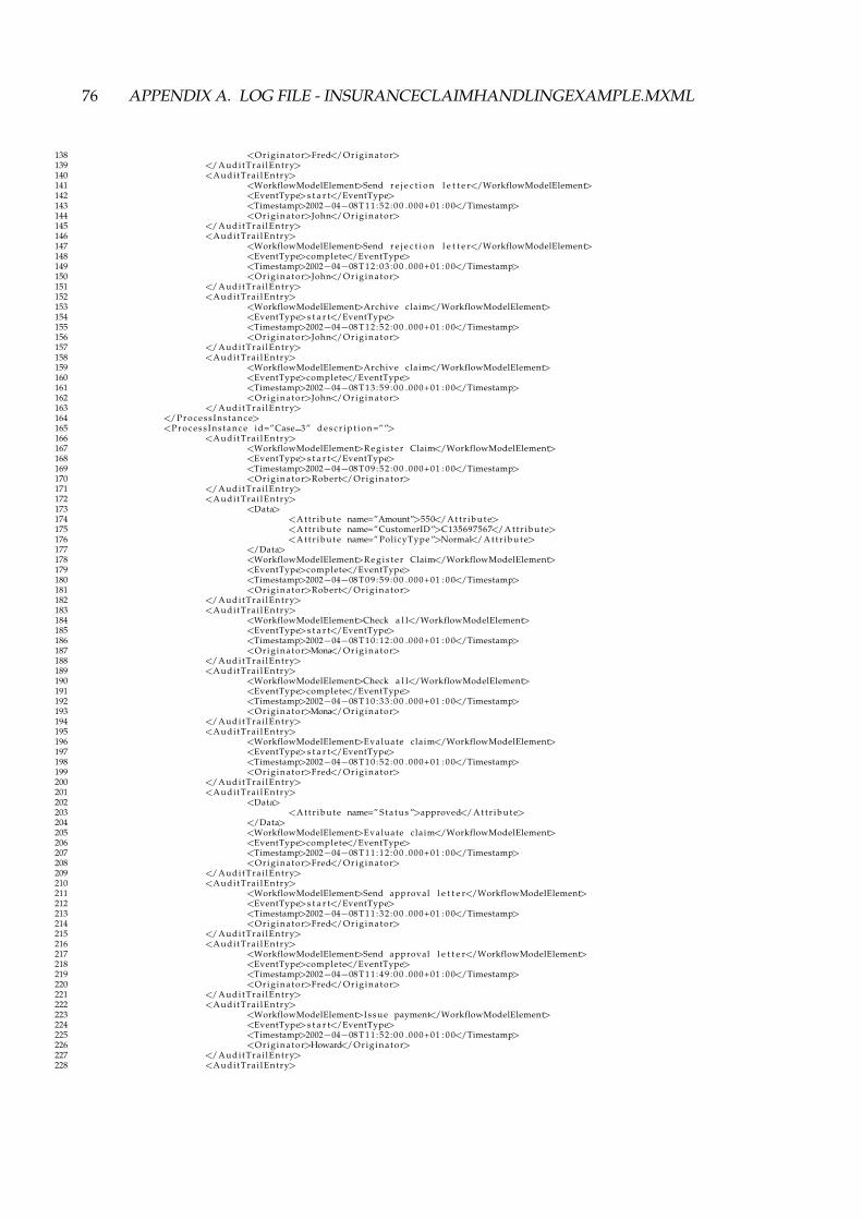
76 APPENDIX A. LOG FILE - INSURANCECLAIMHANDLINGEXAMPLE.MXML

138 <Orig inator>Fred</Orig inator>139 </AuditTrai lEntry>140 <AuditTra i lEntry>141 <WorkflowModelElement>Send r e j e c t i o n l e t t e r</WorkflowModelElement>142 <EventType>s t a r t</EventType>143 <Timestamp>2002−04−08 T 1 1 : 5 2 : 0 0 .000+01 : 0 0</Timestamp>144 <Orig inator>John</Orig inator>145 </AuditTrai lEntry>146 <AuditTra i lEntry>147 <WorkflowModelElement>Send r e j e c t i o n l e t t e r</WorkflowModelElement>148 <EventType>complete</EventType>149 <Timestamp>2002−04−08 T 1 2 : 0 3 : 0 0 .000+01 : 0 0</Timestamp>150 <Orig inator>John</Orig inator>151 </AuditTrai lEntry>152 <AuditTra i lEntry>153 <WorkflowModelElement>Archive claim</WorkflowModelElement>154 <EventType>s t a r t</EventType>155 <Timestamp>2002−04−08 T 1 2 : 5 2 : 0 0 .000+01 : 0 0</Timestamp>156 <Orig inator>John</Orig inator>157 </AuditTrai lEntry>158 <AuditTra i lEntry>159 <WorkflowModelElement>Archive claim</WorkflowModelElement>160 <EventType>complete</EventType>161 <Timestamp>2002−04−08 T 1 3 : 5 9 : 0 0 .000+01 : 0 0</Timestamp>162 <Orig inator>John</Orig inator>163 </AuditTrai lEntry>164 </Pr o ce ss I ns t an c e>165 166 <AuditTra i lEntry>167 <WorkflowModelElement>R e g i s t e r Claim</WorkflowModelElement>168 <EventType>s t a r t</EventType>169 <Timestamp>2002−04−08 T 0 9 : 5 2 : 0 0 .000+01 : 0 0</Timestamp>170 <Orig inator>Robert</Orig inator>171 </AuditTrai lEntry>172 <AuditTra i lEntry>173 <Data>174 <A t t r i b u t e name=”Amount”>550</ A t t r i b u t e>175 <A t t r i b u t e name=”CustomerID”>C135697567</ A t t r i b u t e>176 <A t t r i b u t e name=” PolicyType ”>Normal</ A t t r i b u t e>177 </Data>178 <WorkflowModelElement>R e g i s t e r Claim</WorkflowModelElement>179 <EventType>complete</EventType>180 <Timestamp>2002−04−08 T 0 9 : 5 9 : 0 0 .000+01 : 0 0</Timestamp>181 <Orig inator>Robert</Orig inator>182 </AuditTrai lEntry>183 <AuditTra i lEntry>184 <WorkflowModelElement>Check a l l</WorkflowModelElement>185 <EventType>s t a r t</EventType>186 <Timestamp>2002−04−08 T 1 0 : 1 2 : 0 0 .000+01 : 0 0</Timestamp>187 <Orig inator>Mona</Orig inator>188 </AuditTrai lEntry>189 <AuditTra i lEntry>190 <WorkflowModelElement>Check a l l</WorkflowModelElement>191 <EventType>complete</EventType>192 <Timestamp>2002−04−08 T 1 0 : 3 3 : 0 0 .000+01 : 0 0</Timestamp>193 <Orig inator>Mona</Orig inator>194 </AuditTrai lEntry>195 <AuditTra i lEntry>196 <WorkflowModelElement>Evaluate claim</WorkflowModelElement>197 <EventType>s t a r t</EventType>198 <Timestamp>2002−04−08 T 1 0 : 5 2 : 0 0 .000+01 : 0 0</Timestamp>199 <Orig inator>Fred</Orig inator>200 </AuditTrai lEntry>201 <AuditTra i lEntry>202 <Data>203 <A t t r i b u t e name=” S t a t u s ”>approved</ A t t r i b u t e>204 </Data>205 <WorkflowModelElement>Evaluate claim</WorkflowModelElement>206 <EventType>complete</EventType>207 <Timestamp>2002−04−08 T 1 1 : 1 2 : 0 0 .000+01 : 0 0</Timestamp>208 <Orig inator>Fred</Orig inator>209 </AuditTrai lEntry>210 <AuditTra i lEntry>211 <WorkflowModelElement>Send approval l e t t e r</WorkflowModelElement>212 <EventType>s t a r t</EventType>213 <Timestamp>2002−04−08 T 1 1 : 3 2 : 0 0 .000+01 : 0 0</Timestamp>214 <Orig inator>Fred</Orig inator>215 </AuditTrai lEntry>216 <AuditTra i lEntry>217 <WorkflowModelElement>Send approval l e t t e r</WorkflowModelElement>218 <EventType>complete</EventType>219 <Timestamp>2002−04−08 T 1 1 : 4 9 : 0 0 .000+01 : 0 0</Timestamp>220 <Orig inator>Fred</Orig inator>221 </AuditTrai lEntry>222 <AuditTra i lEntry>223 <WorkflowModelElement>I s sue payment</WorkflowModelElement>224 <EventType>s t a r t</EventType>225 <Timestamp>2002−04−08 T 1 1 : 5 2 : 0 0 .000+01 : 0 0</Timestamp>226 <Orig inator>Howard</Orig inator>227 </AuditTrai lEntry>228 <AuditTra i lEntry>

77

229 <WorkflowModelElement>I s sue payment</WorkflowModelElement>230 <EventType>complete</EventType>231 <Timestamp>2002−04−08 T 1 2 : 0 9 : 0 0 .000+01 : 0 0</Timestamp>232 <Orig inator>Howard</Orig inator>233 </AuditTrai lEntry>234 <AuditTra i lEntry>235 <WorkflowModelElement>Archive claim</WorkflowModelElement>236 <EventType>s t a r t</EventType>237 <Timestamp>2002−04−08 T 1 2 : 2 2 : 0 0 .000+01 : 0 0</Timestamp>238 <Orig inator>Robert</Orig inator>239 </AuditTrai lEntry>240 <AuditTra i lEntry>241 <WorkflowModelElement>Archive claim</WorkflowModelElement>242 <EventType>complete</EventType>243 <Timestamp>2002−04−08 T 1 2 : 5 6 : 0 0 .000+01 : 0 0</Timestamp>244 <Orig inator>Robert</Orig inator>245 </AuditTrai lEntry>246 </Pr o ce ss I ns t an ce>247 248 <AuditTra i lEntry>249 <WorkflowModelElement>R e g i s t e r Claim</WorkflowModelElement>250 <EventType>s t a r t</EventType>251 <Timestamp>2002−04−08 T 0 9 : 5 2 : 0 0 .000+01 : 0 0</Timestamp>252 <Orig inator>Robert</Orig inator>253 </AuditTrai lEntry>254 <AuditTra i lEntry>255 <Data>256 <A t t r i b u t e name=”Amount”>500</ A t t r i b u t e>257 <A t t r i b u t e name=”CustomerID”>C568120443</ A t t r i b u t e>258 <A t t r i b u t e name=” PolicyType ”>Normal</ A t t r i b u t e>259 </Data>260 <WorkflowModelElement>R e g i s t e r Claim</WorkflowModelElement>261 <EventType>complete</EventType>262 <Timestamp>2002−04−08 T 1 0 : 1 1 : 0 0 .000+01 : 0 0</Timestamp>263 <Orig inator>Robert</Orig inator>264 </AuditTrai lEntry>265 <AuditTra i lEntry>266 <WorkflowModelElement>Check pol i cy only</WorkflowModelElement>267 <EventType>s t a r t</EventType>268 <Timestamp>2002−04−08 T 1 0 : 3 2 : 0 0 .000+01 : 0 0</Timestamp>269 <Orig inator>Mona</Orig inator>270 </AuditTrai lEntry>271 <AuditTra i lEntry>272 <WorkflowModelElement>Check pol i cy only</WorkflowModelElement>273 <EventType>complete</EventType>274 <Timestamp>2002−04−08 T 1 0 : 5 9 : 0 0 .000+01 : 0 0</Timestamp>275 <Orig inator>Mona</Orig inator>276 </AuditTrai lEntry>277 <AuditTra i lEntry>278 <WorkflowModelElement>Evaluate claim</WorkflowModelElement>279 <EventType>s t a r t</EventType>280 <Timestamp>2002−04−08 T 1 1 : 2 2 : 0 0 .000+01 : 0 0</Timestamp>281 <Orig inator>Linda</Orig inator>282 </AuditTra i lEntry>283 <AuditTra i lEntry>284 <Data>285 <A t t r i b u t e name=” S t a t u s ”>approved</ A t t r i b u t e>286 </Data>287 <WorkflowModelElement>Evaluate claim</WorkflowModelElement>288 <EventType>complete</EventType>289 <Timestamp>2002−04−08 T 1 1 : 4 7 : 0 0 .000+01 : 0 0</Timestamp>290 <Orig inator>Linda</Orig inator>291 </AuditTra i lEntry>292 <AuditTra i lEntry>293 <WorkflowModelElement>Send approval l e t t e r</WorkflowModelElement>294 <EventType>s t a r t</EventType>295 <Timestamp>2002−04−08 T 1 1 : 5 2 : 0 0 .000+01 : 0 0</Timestamp>296 <Orig inator>Linda</Orig inator>297 </AuditTra i lEntry>298 <AuditTra i lEntry>299 <WorkflowModelElement>Send approval l e t t e r</WorkflowModelElement>300 <EventType>complete</EventType>301 <Timestamp>2002−04−08 T 1 2 : 1 2 : 0 0 .000+01 : 0 0</Timestamp>302 <Orig inator>Linda</Orig inator>303 </AuditTra i lEntry>304 <AuditTra i lEntry>305 <WorkflowModelElement>I s sue payment</WorkflowModelElement>306 <EventType>s t a r t</EventType>307 <Timestamp>2002−04−08 T 1 2 : 2 5 : 0 0 .000+01 : 0 0</Timestamp>308 <Orig inator>Vincent</Orig inator>309 </AuditTrai lEntry>310 <AuditTra i lEntry>311 <WorkflowModelElement>I s sue payment</WorkflowModelElement>312 <EventType>complete</EventType>313 <Timestamp>2002−04−08 T 1 2 : 3 6 : 0 0 .000+01 : 0 0</Timestamp>314 <Orig inator>Vincent</Orig inator>315 </AuditTrai lEntry>316 <AuditTra i lEntry>317 <WorkflowModelElement>Archive claim</WorkflowModelElement>318 <EventType>s t a r t</EventType>319 <Timestamp>2002−04−08 T 1 2 : 5 2 : 0 0 .000+01 : 0 0</Timestamp>

78 APPENDIX A. LOG FILE - INSURANCECLAIMHANDLINGEXAMPLE.MXML

320 <Orig inator>Mona</Orig inator>321 </AuditTrai lEntry>322 <AuditTra i lEntry>323 <WorkflowModelElement>Archive claim</WorkflowModelElement>324 <EventType>complete</EventType>325 <Timestamp>2002−04−08 T 1 3 : 2 3 : 0 0 .000+01 : 0 0</Timestamp>326 <Orig inator>Mona</Orig inator>327 </AuditTrai lEntry>328 </Pr o ce ss I ns t an ce>329 330 <AuditTra i lEntry>331 <WorkflowModelElement>R e g i s t e r Claim</WorkflowModelElement>332 <EventType>s t a r t</EventType>333 <Timestamp>2002−04−08 T 0 9 : 5 2 : 0 0 .000+01 : 0 0</Timestamp>334 <Orig inator>Mona</Orig inator>335 </AuditTrai lEntry>336 <AuditTra i lEntry>337 <Data>338 <A t t r i b u t e name=”Amount”>50</ A t t r i b u t e>339 <A t t r i b u t e name=”CustomerID”>C493823084</ A t t r i b u t e>340 <A t t r i b u t e name=” PolicyType ”>Normal</ A t t r i b u t e>341 </Data>342 <WorkflowModelElement>R e g i s t e r Claim</WorkflowModelElement>343 <EventType>complete</EventType>344 <Timestamp>2002−04−08 T 1 0 : 2 7 : 0 0 .000+01 : 0 0</Timestamp>345 <Orig inator>Mona</Orig inator>346 </AuditTrai lEntry>347 <AuditTra i lEntry>348 <WorkflowModelElement>Check pol i cy only</WorkflowModelElement>349 <EventType>s t a r t</EventType>350 <Timestamp>2002−04−08 T 1 0 : 5 2 : 0 0 .000+01 : 0 0</Timestamp>351 <Orig inator>Howard</Orig inator>352 </AuditTrai lEntry>353 <AuditTra i lEntry>354 <WorkflowModelElement>Check pol i cy only</WorkflowModelElement>355 <EventType>complete</EventType>356 <Timestamp>2002−04−08 T 1 1 : 0 5 : 0 0 .000+01 : 0 0</Timestamp>357 <Orig inator>Howard</Orig inator>358 </AuditTrai lEntry>359 <AuditTra i lEntry>360 <WorkflowModelElement>Evaluate claim</WorkflowModelElement>361 <EventType>s t a r t</EventType>362 <Timestamp>2002−04−08 T 1 1 : 1 7 : 0 0 .000+01 : 0 0</Timestamp>363 <Orig inator>Linda</Orig inator>364 </AuditTrai lEntry>365 <AuditTra i lEntry>366 <Data>367 <A t t r i b u t e name=” S t a t u s ”>r e j e c t e d</ A t t r i b u t e>368 </Data>369 <WorkflowModelElement>Evaluate claim</WorkflowModelElement>370 <EventType>complete</EventType>371 <Timestamp>2002−04−08 T 1 1 : 4 3 : 0 0 .000+01 : 0 0</Timestamp>372 <Orig inator>Linda</Orig inator>373 </AuditTra i lEntry>374 <AuditTra i lEntry>375 <WorkflowModelElement>Send r e j e c t i o n l e t t e r</WorkflowModelElement>376 <EventType>s t a r t</EventType>377 <Timestamp>2002−04−08 T 1 2 : 0 9 : 0 0 .000+01 : 0 0</Timestamp>378 <Orig inator>Vincent</Orig inator>379 </AuditTrai lEntry>380 <AuditTra i lEntry>381 <WorkflowModelElement>Send r e j e c t i o n l e t t e r</WorkflowModelElement>382 <EventType>complete</EventType>383 <Timestamp>2002−04−08 T 1 2 : 2 3 : 0 0 .000+01 : 0 0</Timestamp>384 <Orig inator>Vincent</Orig inator>385 </AuditTrai lEntry>386 <AuditTra i lEntry>387 <WorkflowModelElement>Archive claim</WorkflowModelElement>388 <EventType>s t a r t</EventType>389 <Timestamp>2002−04−08 T 1 2 : 4 2 : 0 0 .000+01 : 0 0</Timestamp>390 <Orig inator>Mona</Orig inator>391 </AuditTrai lEntry>392 <AuditTra i lEntry>393 <WorkflowModelElement>Archive claim</WorkflowModelElement>394 <EventType>complete</EventType>395 <Timestamp>2002−04−08 T 1 3 : 1 3 : 0 0 .000+01 : 0 0</Timestamp>396 <Orig inator>Mona</Orig inator>397 </AuditTrai lEntry>398 </Pr o ce ss I ns t an ce>399 400 <AuditTra i lEntry>401 <WorkflowModelElement>R e g i s t e r Claim</WorkflowModelElement>402 <EventType>s t a r t</EventType>403 <Timestamp>2002−04−08 T 0 7 : 4 3 : 0 0 .000+01 : 0 0</Timestamp>404 <Orig inator>Robert</Orig inator>405 </AuditTrai lEntry>406 <AuditTra i lEntry>407 <Data>408 <A t t r i b u t e name=”Amount”>200</ A t t r i b u t e>409 <A t t r i b u t e name=”CustomerID”>C945675110</ A t t r i b u t e>410 <A t t r i b u t e name=” PolicyType ”>premium</ A t t r i b u t e>

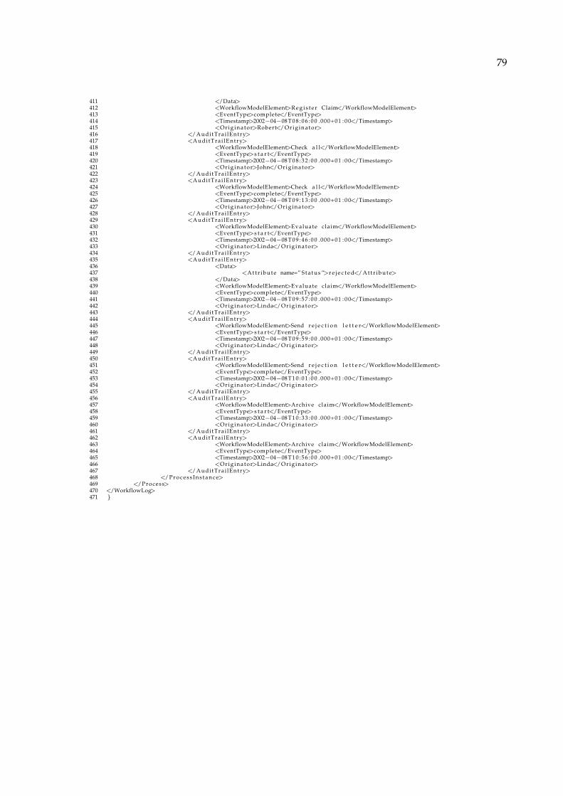
79

411 </Data>412 <WorkflowModelElement>R e g i s t e r Claim</WorkflowModelElement>413 <EventType>complete</EventType>414 <Timestamp>2002−04−08 T 0 8 : 0 6 : 0 0 .000+01 : 0 0</Timestamp>415 <Orig inator>Robert</Orig inator>416 </AuditTrai lEntry>417 <AuditTra i lEntry>418 <WorkflowModelElement>Check a l l</WorkflowModelElement>419 <EventType>s t a r t</EventType>420 <Timestamp>2002−04−08 T 0 8 : 3 2 : 0 0 .000+01 : 0 0</Timestamp>421 <Orig inator>John</Orig inator>422 </AuditTrai lEntry>423 <AuditTra i lEntry>424 <WorkflowModelElement>Check a l l</WorkflowModelElement>425 <EventType>complete</EventType>426 <Timestamp>2002−04−08 T 0 9 : 1 3 : 0 0 .000+01 : 0 0</Timestamp>427 <Orig inator>John</Orig inator>428 </AuditTrai lEntry>429 <AuditTra i lEntry>430 <WorkflowModelElement>Evaluate claim</WorkflowModelElement>431 <EventType>s t a r t</EventType>432 <Timestamp>2002−04−08 T 0 9 : 4 6 : 0 0 .000+01 : 0 0</Timestamp>433 <Orig inator>Linda</Orig inator>434 </AuditTrai lEntry>435 <AuditTra i lEntry>436 <Data>437 <A t t r i b u t e name=” S t a t u s ”>r e j e c t e d</ A t t r i b u t e>438 </Data>439 <WorkflowModelElement>Evaluate claim</WorkflowModelElement>440 <EventType>complete</EventType>441 <Timestamp>2002−04−08 T 0 9 : 5 7 : 0 0 .000+01 : 0 0</Timestamp>442 <Orig inator>Linda</Orig inator>443 </AuditTra i lEntry>444 <AuditTra i lEntry>445 <WorkflowModelElement>Send r e j e c t i o n l e t t e r</WorkflowModelElement>446 <EventType>s t a r t</EventType>447 <Timestamp>2002−04−08 T 0 9 : 5 9 : 0 0 .000+01 : 0 0</Timestamp>448 <Orig inator>Linda</Orig inator>449 </AuditTra i lEntry>450 <AuditTra i lEntry>451 <WorkflowModelElement>Send r e j e c t i o n l e t t e r</WorkflowModelElement>452 <EventType>complete</EventType>453 <Timestamp>2002−04−08 T 1 0 : 0 1 : 0 0 .000+01 : 0 0</Timestamp>454 <Orig inator>Linda</Orig inator>455 </AuditTra i lEntry>456 <AuditTra i lEntry>457 <WorkflowModelElement>Archive claim</WorkflowModelElement>458 <EventType>s t a r t</EventType>459 <Timestamp>2002−04−08 T 1 0 : 3 3 : 0 0 .000+01 : 0 0</Timestamp>460 <Orig inator>Linda</Orig inator>461 </AuditTra i lEntry>462 <AuditTra i lEntry>463 <WorkflowModelElement>Archive claim</WorkflowModelElement>464 <EventType>complete</EventType>465 <Timestamp>2002−04−08 T 1 0 : 5 6 : 0 0 .000+01 : 0 0</Timestamp>466 <Orig inator>Linda</Orig inator>467 </AuditTra i lEntry>468 </Pr o ce ss I ns t an ce>469 </Process>470 </WorkflowLog>471 }

placeholder

Appendix B

User Manual for the Social NetworkMining Plug-in

In this appendix we available an user manual in an effort to present further our plug-in- Organizational Miner Cluster plug-in.

81

User Manual forOrganizational Miner Cluster plug-in

an organizational mining toolimplemented in ProM v6

Cládia Sofia da Costa Alves

June 2010

UNIVERSIDADE TÉCNICA DE LISBOA INSTITUTO SUPERIOR TÉCNICO

Contents

1 Introduction 4

2 Organizational Miner Cluster plug-in 52.1 Getting Start . . . . . . . . . . . . . . . . . . . . . . . . . . . . . . . . 52.2 Organizational Miner Cluster Tabs . . . . . . . . . . . . . . . . . . . . 7

2.2.1 HCA Miner . . . . . . . . . . . . . . . . . . . . . . . . . . . . 72.2.2 Modularity . . . . . . . . . . . . . . . . . . . . . . . . . . . . 122.2.3 Social Network . . . . . . . . . . . . . . . . . . . . . . . . . . 142.2.4 Organizational Network . . . . . . . . . . . . . . . . . . . . . 17

1 IntroductionThis document describes how to use Organizational Miner Cluster plug-in available inProM v.6.

The Organizational perspective from Process Mining is a valuable technique that al-lows studying the social network of an organization. To do so, it provides means tomake an evaluation of networks by mapping and analyzing relationships among people,teams, departments or even entire organizations.

Organizational Miner Cluster plug-in, is a tool of Organizational Mining, which de-rives social networks from event logs generated by Process-aware Information Systems(PAIS). This tool aims to represent a social network not only at the individual level, butalso at the organizational level.

• Individual level derives a flat model, which maps the relationships that existamong the different originators (relationships among people).

• Organizational level takes the previous analysis to a higher level of abstraction. Itmaps the relationships among groups or communities of originators.

The organizational level is achieved using a new technique for identifying commu-nity structures in social networks. A community is defined as a set of nodes denselyconnected with one another; nodes that belong to the same group have a high level ofsimilarity. Different communities are linked by sparse connections. To identify commu-nities, Organizational Miner Cluster plug-in uses an Hierarchical Clustering Agglom-erative , which not only help us identifying communities inside the network, but it alsomake simpler the representation and visualization of the huge amount of data requiredin this kind of analysis. The plug-in also adopts a new concept - Modularity - which isa quality measure for graph clustering. It measures if a specific division of a networkinto a group of communities is good or not, in the sense that the connections inside acommunity are dense and the connections between communities are sparse.

The log file used all along this manual was insuranceClaimHandlingExample.mxmlwhich is available with ProM v5.2

2 Organizational Miner Cluster plug-in

2.1 Getting StartAfter uploading a log file and choosing Organizational Miner Cluster plug-in, will ap-pear a welcome panel. In this panel, user must choose the initial settings for the socialnetwork analysis. Figure 1 shows the initial panel, and as we can observe there arethree main settings: 1) Miner Algorithm 2) Linkage Rule and 3) Tie with Modularity

1. Miner AlgorithmThis option allows the user to choose which kind of analysis he wants to perform.

To derive social networks from event logs, different kinds of metrics have beendeveloped: (1) metrics based on (possible) causality, (2) metrics based on jointcases, (3) metrics based on joint activities, and (4) metrics based on special eventtypes [1].

From these, the Organizational Miner Cluster plug-in supports two of them:

• Working Together Algorithm is a metric based on joint activities. This plug-in only count how frequently individuals work in the same case and mapthese relationships. Two individuals work together if they perform activitiesin the same case of an event log.

• Similar Tasks Algorithm is a metric based on joint activities. The main ideais to determine who performs the same type of activities. To do so, eachindividual has his own profile based on how frequent they conduct specificactivities. Then the profiles are compared to determine the similarity be-tween them. If two individuals have very similar profiles it is probably thatthey work in the same department, for example.

2. Linkage RuleThis option refers to the Hierarchical Clustering Agglomerative Algorithm. Link-age Rules are approaches used to compute the distance between two differentclusters. This plug-in implement three kinds of linkage rules:

a) Single Linkage Rule

b) Complete Linkage Rule

c) Average Linkage Rule

These approaches are further explained in Section 2.2.1

3. Tie with ModularityThis option also refers to the Hierarchical Clustering Agglomerative Algorithm(HAC). In each iteration of HAC the algorithm groups two clusters, and the twoclusters chosen to group are the ones that are more similar. However, sometimesHAC finds more than one couple of clusters to group, which is very common inlarge networks. In this case were facing a situation of tie, and our algorithm canovercome this problem in two different ways:

Figure 1: Initial panel

a) the algorithm will agglomerate the last pair found;

b) the algorithm will use modularity concept. Given a set of couples of clusterswith the same similarity, the algorithm will calculate modularity for eachpossible arrange of clusters, and will choose the one that maximizes themodularity value.

2.2 Organizational Miner Cluster TabsOrganizational Miner Cluster plug-in is composed by four tabs: tab 1 - HCA Algo-rithm, tab 2 - Modularity, tab 3 - Social and tab 4 - Organizational Network. Eachone will be further explained in the following subsections. Each tab deals with differentand specific information as it will be further discussed. For each tab, we first give sometheory notions and basis and then we explain the features and settings of each tab.

2.2.1 HCA Miner

Our plug-in uses Hierarchical Clustering Agglomerative, which means that it start froma single individual, and proceed to successive agglomeration of individuals until a com-munity is found.

HCA Algorithm Given a network with a set of N nodes, the basic process of thehierarchical clustering agglomerative algorithm adopted is as follows:

1. Each node is assigned to a cluster (if there are N nodes, will exist N clusters,each containing just one item). In this step distances (similarities) among clusterscorrespond to the power of the relationship of the nodes they contain;

2. Then the algorithm searches for the most powerful relationship between two clus-ters and merge them into a single cluster, so that now there is one cluster less. Thecalculus of similarity between two individual is calculated differently in WorkingTogether and Similar Tasks metric. In Working Together metric the more oftentwo individuals work together, greater is the power of the relationship betweenthem and greater is their similarity. In Similar Tasks metric the more tasks twoindividuals perform in common, greater is the power of the relationship betweenthem and greater is their similarity.

a) If there are several candidates, i.e., more than a couple of clusters with themost powerful relationship, the decision of which candidates to agglomerateis made according with two options: (1) the algorithm choose the last coupleof clusters found, or (2) the algorithm choose the couple of clusters thatmaximizes the modularity.

3. Compute distances (similarities) between the new cluster and each of the old clus-ters. For this step the algorithm may use one of these methods: single-linkage,complete-linkage or average-linkage;

4. Determine the value of modularity for this number of clusters;

5. Repeat steps 2, 3 and 4 until all items are clustered into a single cluster of size N.

Step 3, the distance between two clusters, can be done in different ways in our ap-proach:

• Single LinkageSingle linkage, also known as the nearest neighbour technique defines similaritybetween two clusters as the distance between the closest pair of elements of thoseclusters. In other words, the distance between two clusters is given by the valueof the shortest link between the clusters.

In the single linkage method, D(r, s) is computed as D(r, s) = Mind(i, j) ,where element i is in cluster r and element j is cluster s. Here the distancebetween every possible object pair (i, j) is computed, where object i is in clusterr and object j is in cluster s. The minimum value of these distances is said to bethe distance among clusters r and s.

At each stage of hierarchical clustering, the clusters r and s , for which D(r, s) isminimum, are merged.

• Complete LinkageThis method is similar to the previous one, but instead of considering the min-imum value, it considers the maximum value. Complete Linkage computes thedistance between two clusters as the distance between the two most distant ele-ments in the two clusters.

• Average LinkageHere the distance between two clusters is defined as the average distance fromany member of one cluster to any member of the other cluster.

In the average linkage method, D(r, s) is computed asD(r, s) = Trs/(Nr∗Ns).Where Trs is the sum of all pair wise distances between cluster r and cluster s.Nr and Ns are the sizes of the clusters r and s respectively.

At each stage of hierarchical clustering, the clusters r and s , for which D(r, s) isthe minimum, are merged.

HCA features Figure 2 shows HCA Algorithm tab that is composed by three mainspanels.

Panel on the right-hand side gives an overview of executed plug-ins, in the figure wecan see that plug-in Organizational Miner Clusters has been executed.

Panel on the middle, depicted in Figure 3 shows the output of HCA Algorithm as atree. The root node, coloured with orange represents the HCA algorithm, child nodesrepresented by blue are each iteration of HCA algorithm, and child nodes representedby green are the clusters achieved in each iteration. New clusters are presented in up-percase, for examples shall we observe the node corresponding to the 3th iteration, theOrganic Unit 1 of this iteration is represented in uppercase because this OrganizationUnit results from the agglomerations of Organization Unit 1 and Organization Unit 4from 2sd iteration.

Finally the panel on the left-hand side is the setting panel where the user can configurethe settings of HCA Algorithm and where some exploiting tools are available.

We will now explain the panel on the left-hand side. HCA tab is the first one availableand is used as the principal one. If the user wants to change the settings initially chosen

in the main panel, he is able to do that here. Figure 4 shows the settings available inthis tab which we will now explain:

1. Social Metric - here the user is able to choose between Working Together metricand Similar Tasks metric;

2. Linkage Rule - this setting allows the user to choose one of the three linkagerules available: Single Linkage, Average Linkage and Complete Linkage

3. Tie break with modularity - This setting is used to choose how HCA will decidewhich candidates to choose in case of tie. If this setting is selected the HCAalgorithm will choose the candidates that maximize modularity. Otherwise it willchoose the last candidates found.

4. Show sub-network - this setting allows the user to analyze a sub-network, i.e.,given set of clusters, the user can choose one in particular and analyze this clusterindividually and analyze the nodes that compose this cluster. For example, let’sassume that we want to analyze the Organization Unit 1 from the fourth iteration.Figure 4 shows the result, and as we can see this functionality gives us the outputin two different ways: (1) as a matrix, were the value of each cell corresponds tothe power of the relationship, (2) or as a graph were the power of the relationshipis depicted as the link label.

5. Button Collapse All, collapses all the nodes of the tree shown in the middle paneland only shows the child’s at level 1.

6. Button Expand All, expands all the nodes of the tree shown in the middle panel.

7. Button Calculate, calculates HCA Algorithm according to the options selected inthe setting panel.

Figure 2: HAC tree

Figure 3: HAC tab - middle panel

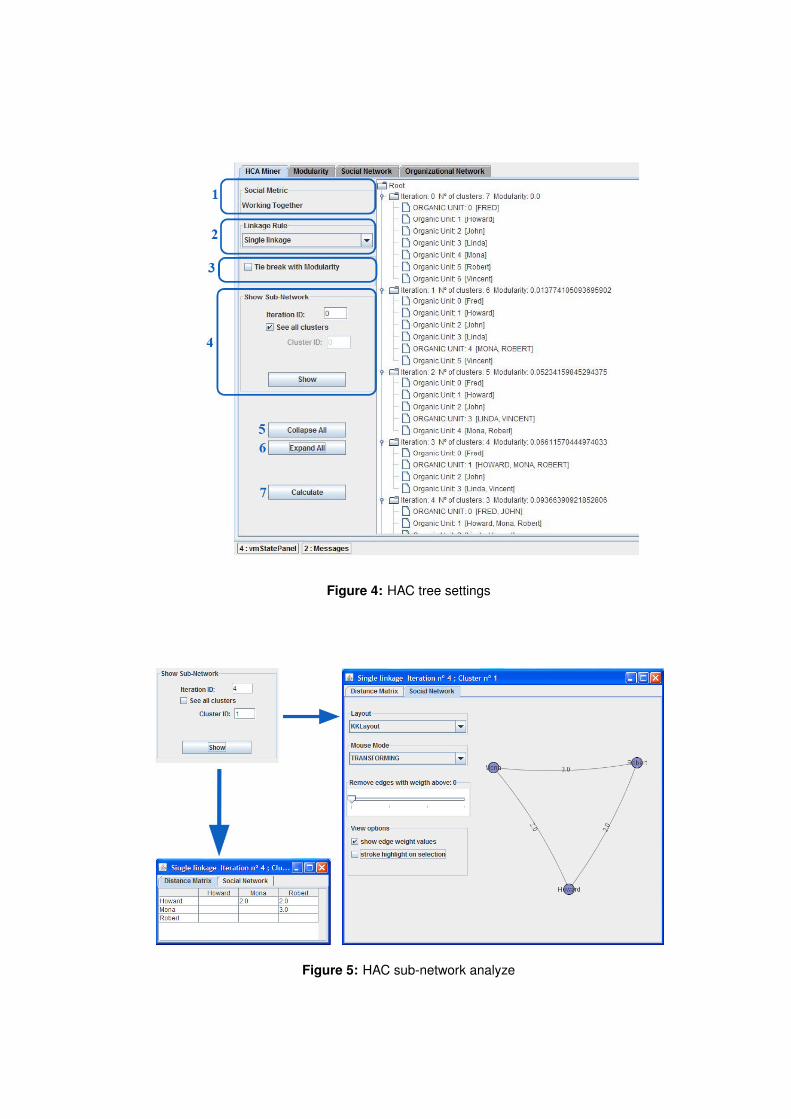
Figure 4: HAC tree settings

Figure 5: HAC sub-network analyze

2.2.2 Modularity

Modularity is a quality measure for graph clustering. It measures if a specific division ofa network into a group of communities is good or not, in the sense that the connectionsinside a community are dense and the connections among communities is sparse.

The needed to use this concept arrived because on of the most important and serioushandicaps of Hierarchical Clustering Algorithms. All these kind of algorithms have thedisadvantage of not providing any guidance of how many communities a network shouldbe split into. For example, in a Agglomerative Clustering approach, the algorithm iter-ates from one element per cluster to a cluster containing all the elements, and the userdoes not now, which of the several iterations is the best one, the one that matches withthe reality.

To address this problem we adopted Modularity concept which has recently emerged[2, 3].

Next we will explain how the modularity is calculated.

Definition of Modularity To help explaining how to compute modularity, we willmake some assumptions:

• Assume a network composed of N vertices connected by m links or edges;

• LetAij be an element of the adjacency matrix (symmetric matrix) of the network,which gives the number of edges between vertices i and j, i.e.; the power of therelationship between element i and element j.

• Finally, suppose we are given a candidate division of the vertices into Nc commu-nities [4].

The modularity of this division is defined to be the fraction of the edges that fallwithin the given groups minus the expected such fraction if edges were distributed atrandom. The fraction of the edges that fall within the given groups is expressed by Aij .And the expected number of edges falling between two vertices i and j, at random, iskikj/2m where ki is the degree of vertex i and kj is the degree of vertex j. Hencethe actual minus expected number of edges between the same two vertices giver by thefollowing equation:

q = Aij −kikj

2m(1)

Summing over all pairs of vertices in the same group, the modularity, denoted Q, isthen given by the following equation:

Q =1

2m

∑

ij

[Aij −

kikj

2m

]δ(ci, cj) (2)

Where ci is the group to which vertex i belongs and cj is the group to which ver-tex j belongs. δ(ci, cj) = 1 if vertex i and vertex j belong to the same cluster, andδ(ci, cj) = 0, if they belong to different clusters.

The value of the modularity lies in the range [-1,1]. It is positive if the number ofedges within groups exceeds the number expected on the basis of chance.

Figure 6: Modularity chart

Modularity features We will now explain the features available in Modularity Tab.In the settings panel we have three main features which are merely informative, as wecan see in Figure 6.

1. Social metric informs the metric that was selected in the main panel or in HCAtab. Note that in this tab the user are not able to change this feature.

2. Linkage rules informs the linkage rule that was selected in the main panel or inHCA tab. Note that in this tab the user are not able to change this feature.

3. Information informs which iteration has the highest value and the respectivevalue

Figure 7: Social Network tab

2.2.3 Social Network

Social Network tab, offers to the user, an individual perspective. This functionality ofthe plug-in, derives from the event log, a flat model where the user can analyze howindividuals of the network are connected between one another. Figure 7 representsSocial Network tab and as we can see, the network is depicted as a graph, where eachnode represents an individual and the links connecting nodes represent the relationshipthat exists between them.

Each node is represented by one colour, and nodes from the same cluster are repre-sented by the same colour. For example, in Figure 7 we can see the social network ofthe 2nd iteration of HCA Algorithm. Nodes Linda and Vincent are both represented byorange because they belong to the same cluster.

This perspective allows us to see the relationship among originators, and to see whichof them belong to the same clusters. However with this perspective we are not ableto analyze the relationships among clusters. We overcome this issue with a secondperspective - Organizational Network - which is available in the fourth and last tab.

Social Network features As the other tab, this one is also composed by three pan-els. We will explain the settings panel, represented in Figure 8, and how each featureswork.

1. Social metric informs which metric was selected in the main panel or in HCAtab. Note that in this tab the user are not able to change this feature.

2. Linkage rules informs which linkage rule that was selected in the main panel orin HCA tab. Note that in this tab the user are not able to change this feature.

3. Layout: This feature available five algorithms use to draw undirected graphs .These algorithms calculate the layout of a graph only using information contained

within the structure of the graph itself, rather than relying on domain-specificknowledge. Graphs drawn with these algorithms tend to be aesthetically pleasing,exhibit symmetries, and tend to produce crossing-free layouts for planar graphs.The five different types of algorithms used in this plug-in are:

• KKLayout also known as Kamada-Kawai layout, attempts to position nodeson the space so that the geometric (Euclidean) distance among them is asclose as possible to the graph-theoretic (path) distance among them.

• Circle layout: arranges all the node randomly into a circle, with constantspacing between each neighbour node.

• FRLayout also known as Fruchterman-Rheingold layout

• SpringLayout: it is a force-directed layout algorithm designed to simulate asystem of particles each with some mass. The vertices simulate mass pointsrepelling each other and the edges simulate springs with attracting forces.

• ISOMLayout: it a layout for self-organizing graphs. This is a neural net-work technique that arranges the data according to a low dimensional struc-ture. The original data is partitioned into as many homonogeneous clustersas there are units, in such way that close clusters contain close data points inthe original space.

4. Mouse Mode: this features has two options: (1) Transforming, which drags allthe graph all around the screen; and (2) Picking, which drags only a specific node.

5. HCA Algorithm Iteration: shows the social network that corresponds to theiteration of HCA algorithm selected with the slide bar.

6. Remove Edges: with the slide bar the user can choose a threshold. All the edgeswith label above the threshold will not be drawn.

7. View Options

• show edge weights: if checked, edges are labelled with their weights. Oth-erwise, edges are not labelled.

• stroke highlight on selection: if checked, edges are drawn using thick solidlines, the thickness of each line is proportional to its weight. As bigger isthe weight, thicker will be the line.

• group clusters: if checked, nodes belonging to the same cluster will bedrawn closed to each other as we can see in Figure 8.

Figure 8: Social Network settings

Figure 9: Group clusters

Figure 10: Organizational Network tab

2.2.4 Organizational Network

This perspective allows the user to identify teams in social network and to analyze therelationships that exists among those teams. Figure 10 represents Organizational Net-work tab and as we can see the network is depicted as a graph, where each node rep-resents one team and the links connecting nodes represent the relationship that existsamong them.

Figure 10 corresponds to the Organizational perspective of Figure 7. Notice thatnodes from the same cluster, in social perspective, have the same colour as their cluster,in the organizational perspective. For example, Linda and Vincent are represented withthe colour orange as well is their cluster in the organizational perspective.

The features of this tab are similar to the features available in Social Network Tab.

References[1] W.M.P. van der Aalst, M. Song, Mining social networks: Uncovering interaction

patterns in business processes, in: J. Desel, B. Pernici, M. Weske (Eds.), Interna-tional Conference on Business Process Management (BPM 2004), Lecture Notes inComputer Science, vol. 3080, Springer, Berlin, 2004, pp. 244-260

[2] M. E. J. Newman, Detecting community structure in networks. Eur. Phys. J. B 38,321-330 (2004)

[3] M. E. J. Newman, Modularity and community structure in networks. Proceedingsof the National Academy of Science (USA), 103, 8577-8582 (2006)

[4] Clauset, A., Newman, M. E. J., and Moore, C. (2004). Finding community structurein very large networks. Physical Review E, 70:06111.

social network analysis for business process discovery · resumo ap erspectiva organizacional da...

Documents