TILS619 Time Series Analysis

Matti Vihola

Spring 2017

Contents

1 Introduction 31.1 Time series data . . . . . . . . . . . . . . . . . . . . . . . . . . . 31.2 Objectives . . . . . . . . . . . . . . . . . . . . . . . . . . . . . . . 31.3 Time series models . . . . . . . . . . . . . . . . . . . . . . . . . . 41.4 Basic summary statistics . . . . . . . . . . . . . . . . . . . . . . . 51.5 Stationarity . . . . . . . . . . . . . . . . . . . . . . . . . . . . . . 61.6 White noise . . . . . . . . . . . . . . . . . . . . . . . . . . . . . . 71.7 Estimation of stationary mean and autocorrelation . . . . . . . . 8

2 Exploratory data analysis, trends and cycles 82.1 Smoothing . . . . . . . . . . . . . . . . . . . . . . . . . . . . . . . 92.2 Cycles . . . . . . . . . . . . . . . . . . . . . . . . . . . . . . . . . 112.3 Trends . . . . . . . . . . . . . . . . . . . . . . . . . . . . . . . . . 14

3 Spectral analysis 173.1 The periodogram . . . . . . . . . . . . . . . . . . . . . . . . . . . 173.2 Leakage and tapering . . . . . . . . . . . . . . . . . . . . . . . . . 233.3 Spectrogram . . . . . . . . . . . . . . . . . . . . . . . . . . . . . . 24

4 Box-Jenkins models 274.1 Moving average (MA) . . . . . . . . . . . . . . . . . . . . . . . . 274.2 Autoregressive (AR) . . . . . . . . . . . . . . . . . . . . . . . . . 304.3 Invertibility of MA . . . . . . . . . . . . . . . . . . . . . . . . . . 334.4 Autoregressive moving average (ARMA) . . . . . . . . . . . . . . 344.5 Integrated models . . . . . . . . . . . . . . . . . . . . . . . . . . . 364.6 Seasonal dependence . . . . . . . . . . . . . . . . . . . . . . . . . 38

5 Parameter estimation 41

Copyright c© 2017 by Matti Vihola and University of Jyvaskyla

5.1 Mean and trends . . . . . . . . . . . . . . . . . . . . . . . . . . . 415.2 Autoregressive model . . . . . . . . . . . . . . . . . . . . . . . . . 415.3 General ARMA . . . . . . . . . . . . . . . . . . . . . . . . . . . . 45

6 Model selection tools 466.1 Non-stationarity . . . . . . . . . . . . . . . . . . . . . . . . . . . . 466.2 Autocorrelation . . . . . . . . . . . . . . . . . . . . . . . . . . . . 476.3 Partial autocorrelation function . . . . . . . . . . . . . . . . . . . 486.4 Information criteria . . . . . . . . . . . . . . . . . . . . . . . . . . 50

7 Model diagnostics 527.1 Residuals . . . . . . . . . . . . . . . . . . . . . . . . . . . . . . . 527.2 Residual tests . . . . . . . . . . . . . . . . . . . . . . . . . . . . . 537.3 Overfitting . . . . . . . . . . . . . . . . . . . . . . . . . . . . . . . 55

8 Forecasting 558.1 Autoregressive process . . . . . . . . . . . . . . . . . . . . . . . . 568.2 General ARIMA . . . . . . . . . . . . . . . . . . . . . . . . . . . 57

9 Spectrum of a stationary process 589.1 Spectral density . . . . . . . . . . . . . . . . . . . . . . . . . . . . 589.2 Spectral distribution function (not examinable) . . . . . . . . . . 609.3 Spectral density of ARMA process . . . . . . . . . . . . . . . . . 619.4 Linear time invariant filters (not examinable) . . . . . . . . . . . . 619.5 Spectrum estimation . . . . . . . . . . . . . . . . . . . . . . . . . 639.6 Parametric spectrum estimation . . . . . . . . . . . . . . . . . . . 69

10 State-space models 7110.1 Linear-Gaussian state-space model . . . . . . . . . . . . . . . . . 7110.2 State inference in linear-Gaussian state-space model . . . . . . . . 7510.3 Maximum likelihood inference in linear-Gaussian state-space models 8010.4 On Bayesian inference for linear-Gaussian state-space models . . . 8310.5 Hidden Markov models . . . . . . . . . . . . . . . . . . . . . . . . 8510.6 General state-space models . . . . . . . . . . . . . . . . . . . . . . 8610.7 State inference in general state-space models . . . . . . . . . . . . 8910.8 On Bayes inference in general state-space models . . . . . . . . . 90

2

Outline of topics & relevant literature

Topics:1. Introduction, basics2. Exploratory data analysis, trends & cycles3. Spectral analysis4. Box-Jenkins models5. Parameter estimation6. Model identification, diagnostics, forecasting7. State-space models

Literature• Brockwell & Davis: Time Series: Theory and Methods, Springer, 1991.• Shumway & Stoffer: Time Series Analysis and Its Applications (With R

Examples), Springer, 2010.• Cryer & Chan: Time Series Analysis With Applications in R, Springer

2008.• Durbin & Koopman: Time Series Analysis by State Space Methods, Oxford

University Press, 2001.

1 Introduction

1.1 Time series data

Time series is a sequential data x1, . . . , xn collected at increasing time instantst1 < · · · < tn, respectively. Our primary focus in this course is on series which are• univariate (real-valued) and• uniformly sampled (i.e. the time points are equally spaced, ti+1 − ti =

const).The last point also suggests that the series are complete, with no missing obser-vations.

In some applications we might encounter vector-valued or irregularly sam-pled time series, perhaps with missing data. The state-space techniques which wediscuss later in the course are available also in this context.

1.2 Objectives

Time series data arise in various contexts. For example• Rainfall or average temperature over months• Average house prices or stock prices• EEG or audio signals. . .

There are many possible objectives of the analysis.

3

1946 1948 1950 1952 1954 1956 1958 1960

20

22

24

26

28

30

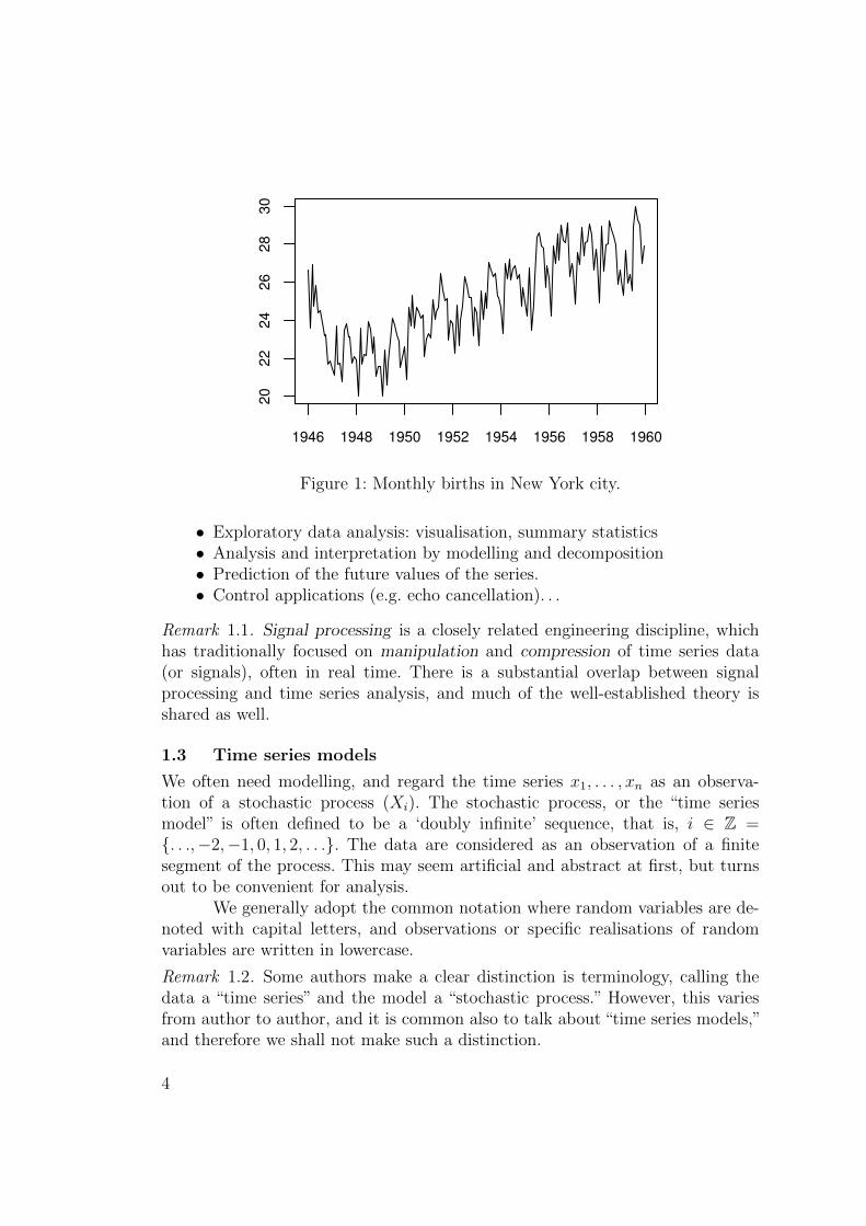
Figure 1: Monthly births in New York city.

• Exploratory data analysis: visualisation, summary statistics• Analysis and interpretation by modelling and decomposition• Prediction of the future values of the series.• Control applications (e.g. echo cancellation). . .

Remark 1.1. Signal processing is a closely related engineering discipline, whichhas traditionally focused on manipulation and compression of time series data(or signals), often in real time. There is a substantial overlap between signalprocessing and time series analysis, and much of the well-established theory isshared as well.

1.3 Time series models

We often need modelling, and regard the time series x1, . . . , xn as an observa-tion of a stochastic process (Xi). The stochastic process, or the “time seriesmodel” is often defined to be a ‘doubly infinite’ sequence, that is, i ∈ Z ={. . .,−2,−1, 0, 1, 2, . . .}. The data are considered as an observation of a finitesegment of the process. This may seem artificial and abstract at first, but turnsout to be convenient for analysis.

We generally adopt the common notation where random variables are de-noted with capital letters, and observations or specific realisations of randomvariables are written in lowercase.

Remark 1.2. Some authors make a clear distinction is terminology, calling thedata a “time series” and the model a “stochastic process.” However, this variesfrom author to author, and it is common also to talk about “time series models,”and therefore we shall not make such a distinction.

4

0 5 10 15 20 25 30

−2

−1

01

2

Figure 2: Realisations of white noise (Xi)i.i.d.∼ N(0, 1)

0 5 10 15 20 25 30

−4

−2

02

4

Figure 3: Realisations of random walk Xi =∑i

j=1Wj, (Wj)i.i.d.∼ N(0, 1)

Remark 1.3. Stochastic process means that the random variables Xi may, andoften do, exhibit (non-negligible) dependencies. In probability terminology, all Xi

are defined on a common probability space.

1.4 Basic summary statistics

Suppose (Xi)i∈I is a stochastic process, and I ⊂ Z.

Definition 1.4 (Mean). The mean (µi) of (Xi) consists of the mean of eachindividual variable Xi:

µi := E[Xi] for all i ∈ I

Definition 1.5 (Autocovariance and autocorrelation). The autocovariance andautocorrelation are covariance and correlation of a (finite variance) time series

5

0 5 10 15 20 25 30

−6

−2

24

6

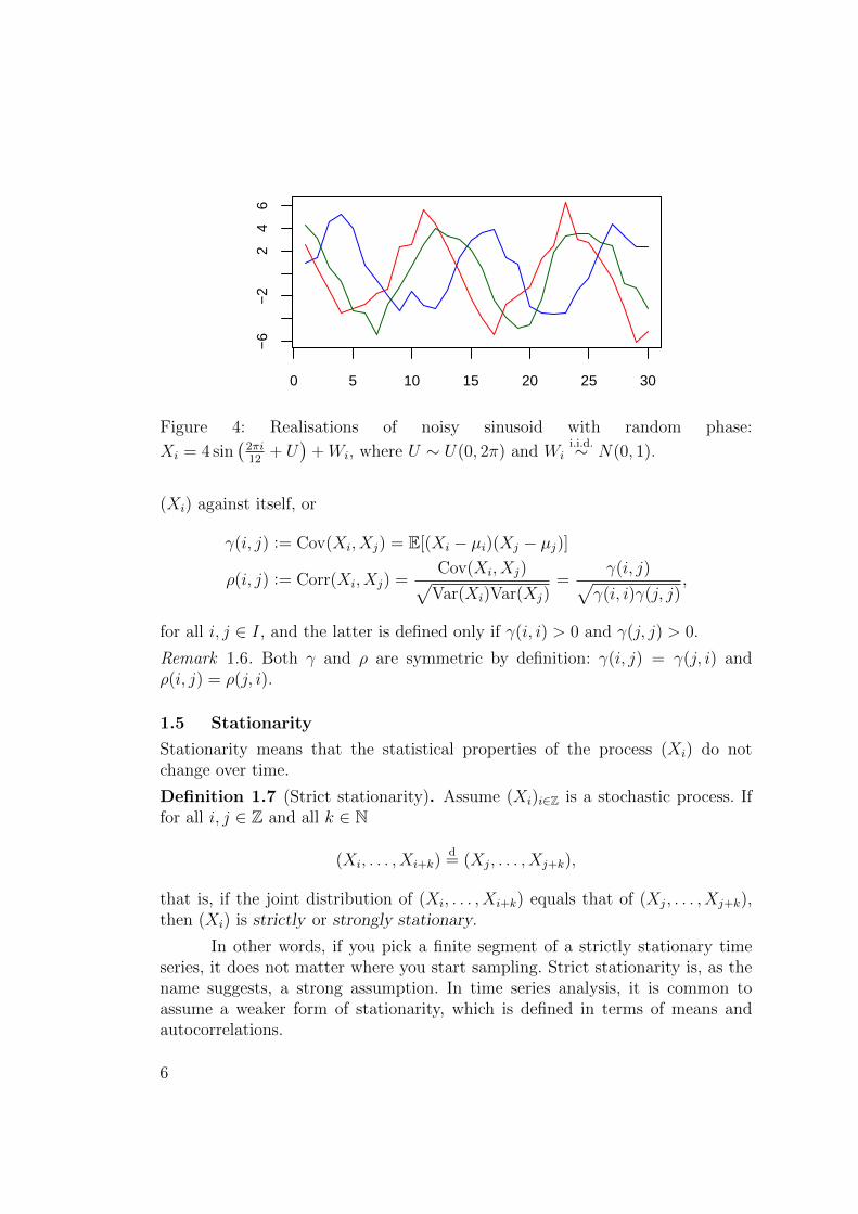
Figure 4: Realisations of noisy sinusoid with random phase:

Xi = 4 sin(2πi12

+ U)

+Wi, where U ∼ U(0, 2π) and Wii.i.d.∼ N(0, 1).

(Xi) against itself, or

γ(i, j) := Cov(Xi, Xj) = E[(Xi − µi)(Xj − µj)]

ρ(i, j) := Corr(Xi, Xj) =Cov(Xi, Xj)√

Var(Xi)Var(Xj)=

γ(i, j)√γ(i, i)γ(j, j)

,

for all i, j ∈ I, and the latter is defined only if γ(i, i) > 0 and γ(j, j) > 0.

Remark 1.6. Both γ and ρ are symmetric by definition: γ(i, j) = γ(j, i) andρ(i, j) = ρ(j, i).

1.5 Stationarity

Stationarity means that the statistical properties of the process (Xi) do notchange over time.

Definition 1.7 (Strict stationarity). Assume (Xi)i∈Z is a stochastic process. Iffor all i, j ∈ Z and all k ∈ N

(Xi, . . . , Xi+k)d= (Xj, . . . , Xj+k),

that is, if the joint distribution of (Xi, . . . , Xi+k) equals that of (Xj, . . . , Xj+k),then (Xi) is strictly or strongly stationary.

In other words, if you pick a finite segment of a strictly stationary timeseries, it does not matter where you start sampling. Strict stationarity is, as thename suggests, a strong assumption. In time series analysis, it is common toassume a weaker form of stationarity, which is defined in terms of means andautocorrelations.

6

Question. Which of the processes in Figures 2–4 could be stationary? What aboutFigure 1?

Definition 1.8 (Stationarity). Assume (Xi)i∈Z is a stochastic process. If(i) (Xi) is constant mean, µ = µi for all i ∈ Z, and(ii) the autocovariance depends only in the difference of the indices,

γ(i+ k, i) = γ(i, i+ k) = γ(0, k) for all i ∈ Z and all k ∈ N,

then (Xi) is stationary. For stationary time series, we denote γk := γ(0, k).

The property above is also called weak sense stationarity, or second orderstationarity in the literature.

Proposition 1.9. If (Xi)i∈Z is stationary, then(i) Var(Xi) = γ0 for all i ∈ Z, and

(ii) if γ0 > 0, then ρk := γkγ0

= ρ(i, i+ k) for all i ∈ Z and k ∈ N.

Theorem 1.10. If (Xi) is a Gaussian process, that is, the joint distributions of(Xi, . . . , Xi+k) are multivariate Gaussian for all i ∈ Z and all k ∈ N, then (weak)stationarity is equivalent to strict stationarity.

Proof. Recall that a Gaussian process is fully determined by the mean and co-variance structure.

Warning. The claim of Theorem 1.10 does not hold in general if eachXi is Gaussian marginally.

1.6 White noise

Definition 1.11. A process (Xi) consisting of i.i.d. random variablesX0, X±1, X±2, . . . is called white1 noise if µi = 0 and Var(Xi) = σ2 ∈ (0,∞).We write (Xi) is WN(σ2).

Definition 1.12. If (Xi)i.i.d.∼ N(0, σ2), then (Xi) is Gaussian white noise.

White noise, as such, is not a very interesting model—i.i.d. measurementscould be analysed with standard methods. However, it is the ‘driving randomness’in many time series models.

Remark 1.13. Sometimes white noise is defined so that (Xi) need not be in-dependent or identically distributed, but instead only assuming that the ran-dom variables hare zero mean and common variance, and to be uncorrelated:Cov(Xi, Xj) = 0 for i 6= j. We do not pursue this generalisation further.

1. The ‘white’ comes from the analogy of electromagnetic radiation in light, which has ‘equal’amount of all colours (frequencies). . .

7

1.7 Estimation of stationary mean and autocorrelation

In general, when the mean of the time series is constant, µi = µ, the obviousestimator of µ is the sample mean of the process

x =1

n

n∑j=1

xj.

Definition 1.14. The sample autocovariance and sample autocorrelation ofx1, . . . , xn for lags k = 0, . . . , n− 1 are

γk :=1

n

n−k∑i=1

(xi+k − x)(xi − x) and ρk :=γkγ0,

respectively, where ρk are defined assuming γ0 > 0.

Plot of ρk with respect to k ≥ 0 is sometimes called the correlogram.

Remark 1.15. The estimator γk is biased, but the common factor n−1 ensuresthat (γk) is positive semi-definite,

n∑i=1

n∑j=1

aiaj γ|i−j| ≥ 0, (1)

for all n and vectors a = (a1, . . . , an) ∈ Rn. In fact, if γ0 > 0, then the inequalityin (1) is strict if a 6= 0.

Remark 1.16. Sample autocovariance/correlation can be always calculated, butit may not be meaningful if the process is not stationary. In fact, slowly decayingsample autocorrelation suggests a possible non-stationarity.

Theorem 1.17. Assume (Xi) is WN(σ2) with EX4i < ∞. Then, the sample

autocorrelation ρ(n)k calculated from X1, . . . , Xn satisfies for any h > 1,

√n(ρ

(n)1 , . . . , ρ

(n)h )

n→∞−−−→ N(0, Ih) in distribution,

where Ih ∈ Rh×h is the identity matrix.

For a proof, see Brockwell and Davis, Theorem 7.2.1.

Remark 1.18. The confidence intervals shown by R function acf by default arebased on this asymptotic result. That is, if (Xi) is WN, then each ρ

(n)k is nearly

N(0, n−1) for large n.

2 Exploratory data analysis, trends and cycles

The first step in practical time series data analysis is (as usual) to inspect thedata visually. When inspecting trend behaviour, smoothed versions of the processmight be informative.

8

0 2 4 6 8 10 12 14

−0.4

0.0

0.4

0.8

0 2 4 6 8 10 12 14

0.0

0.4

0.8

0 10 20 30 40 50

0.0

0.4

0.8

0 10 20 30 40 50

−0.5

0.5

1.0

Figure 5: Top: ACF of standard Gaussian white noise with n = 30 (left) andn = 300 (right); bottom: ACF of random walk (left) and random sine (right)with n = 30, 000.

2.1 Smoothing

Definition 2.1 (Moving average). Assume m ∈ N, and define for m < i < n−m

xi =1

2m+ 1

i+m∑j=i−m

xj.

This is a moving average with window size 2m+ 1.

plot(AirPassengers); w <- 13

win <- rep(1/w, w)

AP_smoothed <- filter(AirPassengers, win, sides=2)

lines(AP_smoothed, col="red")

Instead of taking simple average over the window, more weight can begiven to some samples, typically the ones closer to the centre.

Definition 2.2 (Weighted moving average). Assume k ∈ N and supposeθ0, . . . , θ2k are non-negative numbers with

∑j θj = 1. Then, the weighted moving

average is

xi =2k∑j=0

θjxi−k+j, for k < i < n− k.

9

1950 1952 1954 1956 1958 1960

100

300

500

Figure 6: R data AirPassengers and its smoothed version with window size 13(dashed red).

Note that the simple moving average has θ0 = · · · = θ2k = (2k + 1)−1.

Example 2.3 (Hamming window2). Define the weights for j = 0, . . . , 2n as

θj = α− β cos

(2πj

2n

), and θj =

θj∑2nk=0 θk

with α = 0.54 and β = 1− α.

Exponential smoothing is another popular and simple method:

Definition 2.4 (Exponential smoothing). Let β ∈ (0, 1), set x1 = x1 and thenrecursively

xk = (1− β)xk + βxk−1, k = 2, . . . , n.

Remark 2.5. We may write the exponential smoothing as

xk =k−1∑i=0

θixk−i, where θi :=

{βi, i = k − 1

(1− β)βi, i < k − 1,

which is (for large k) an exponentially weighted moving average.

b <- 0.9

AP_ewma <- (1-b)*filter(AirPassengers, b, method="r",

init=AirPassengers[1]/(1-b))

2. There are some theoretical justifications why this particular weighing might be preferable,but there are other window functions as well. . .

10

0 2 4 6 8 10 12 14

0.0

20.0

60.1

0

Figure 7: The hamming window weights θi with n = 7.

2.2 Cycles

Cyclic behaviour is particularly common in time-series analysis. Simple sinusoidalmean model can be expressed easily by linear regression, by noticing that we canwrite

β sin(2πt+ φ) = β1 cos(2πt) + β2 sin(2πt),

with the following one-to-one correspondence3 between (β, φ) and (β1, β2):

β1 = β sin(φ), β2 = β cos(φ), and

β =√β21 + β2

2 , φ = arctan(β1/β2).

Example 2.6. Fitting sinusoidal model to temperature time series.

library(TSA); data(tempdub)

t <- as.numeric(time(tempdub))

x1 <- cos(2*pi*t); x2 <- sin(2*pi*t)

model <- lm(tempdub ~ x1+x2)

par(mfrow=c(3,1))

plot(tempdub, col="red", type="p", ylab="Temperature",

main="Data & fitted(model)")

lines(t, fitted(model), type="l")

plot(t, residuals(model), type="p", xlab="Time",

3. Recall that sin(x+ y) = cos(x) sin(y) + sin(x) cos(y).

11

Data & fitted(model)

Tem

pera

ture

1964 1966 1968 1970 1972 1974 1976

10

30

50

70

1964 1966 1968 1970 1972 1974 1976

−1

00

5

residuals(model)

Te

mp

era

ture

diff.

5 10 15 20

−0.2

0.0

0.2

Series residuals(model)

AC

F

Figure 8: Sinusoidal model fitted to temperature data.

main="residuals(model)", ylab="Temperature diff.")

acf(residuals(model))

The pure sinusoidal model is rarely appropriate, but seasonal variation is,in general, very common. The seasonal means model assumes that

µi = µi+kf , for all 1 ≤ i ≤ f and 0 ≤ k ≤ ni,

where f is the frequency of the data, that is, the length of the period (e.g. f = 12with monthly data), and ni :=

⌊n−if

⌋. If the total number of points n = mf , then

ni = m− 1.The seasonal means can be estimated with the obvious estimator

µi =1

ni + 1

ni∑k=0

xi+kf .

Example 2.7. The temperature data with seasonal means:

12

Data & fitted(model)Tem

pera

ture

1964 1966 1968 1970 1972 1974 1976

10

30

50

70

1964 1966 1968 1970 1972 1974 1976

−5

05

10

residuals(model)

Te

mp

era

ture

diff.

5 10 15 20

−0.1

50.0

00.1

5

Series res_

AC

F

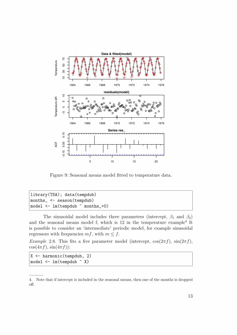
Figure 9: Seasonal means model fitted to temperature data.

library(TSA); data(tempdub)

months_ <- season(tempdub)

model <- lm(tempdub ~ months_+0)

The sinusoidal model includes three parameters (intercept, β1 and β2)and the seasonal means model f, which is 12 in the temperature example4 Itis possible to consider an ‘intermediate’ periodic model, for example sinusoidalregressors with frequencies mf , with m ≤ f .

Example 2.8. This fits a five parameter model (intercept, cos(2πf), sin(2πf),cos(4πf), sin(4πf)):

X <- harmonic(tempdub, 2)

model <- lm(tempdub ~ X)

4. Note that if intercept is included in the seasonal means, then one of the months is droppedoff.

13

Data & fitted(model)

Tem

pera

ture

1964 1966 1968 1970 1972 1974 1976

10

30

50

70

1964 1966 1968 1970 1972 1974 1976

−5

05

10

residuals(model)

Te

mp

era

ture

diff.

5 10 15 20

−0.1

50.0

00.1

5

Series residuals(model)

AC

F

Figure 10: Cosine model with intercept and regressorscos(2πt), sin(2πt), cos(4πt), sin(4πt).

Question. What happens if we would regress here with respect to the interceptplus sin(2πt), cos(2πt), . . . , sin(10πt), cos(10πt) and sin(12πt)? How that com-pares with seasonal means?

Remark 2.9. There are many cases where exactly periodic mean models may notbe appropriate, but which still have periodic dependencies. We will return to suchcases later.

2.3 Trends

It is not uncommon that a time-series contains a trend, which is often of interest.Linear regression methods may be used to capture parametric trends. With alinear trend, an alternative is to consider differencing.

Definition 2.10 (Difference series). Suppose (xi)i=1,...,n is a time series, then

∇xi := xi − xi−1, where i = 2, . . . , n,

is the difference series corresponding (xi). The higher order differences are defined

14

1950 1952 1954 1956 1958 1960

5.0

6.0

0.0 0.5 1.0 1.5

−0.2

0.2

0.6

1.0

1950 1952 1954 1956 1958 1960

−0.3

0.0

0.2

0.0 0.5 1.0 1.5

−0.4

0.2

0.8

1950 1952 1954 1956 1958 1960

−0.2

0.0

0.2

0.0 0.5 1.0 1.5

−0.2

0.4

0.8

Figure 11: Linear trend in the log-AirPassengers data, the detrended series andthe differenced series, with their ACFs.

as

∇dxi := ∇d−1xi −∇d−1xi−1, where i = d+ 1, . . . , n.

x <- log(AirPassengers); t <- as.numeric(time(x))

model <- lm(x ~ t)

detrend <- ts(resid(model),start=start(x),deltat=deltat(x))

dx <- diff(x)

In case of seasonal dependence, it may be useful to consider lagged differ-ences.

Definition 2.11 (Lagged differences). Suppose (xi)i=1,...,n is a time series ands ≥ 1, then

∇sxi = xi − xi−s, where i = s+ 1, . . . , n

is the s:th lagged difference sequence, and the higher-order lagged differences

∇dsxi := ∇d−1

s xi −∇d−1s xi−s.

15

Time

1950 1954 1958

0.0

0.2

0.0 0.5 1.0 1.5

−0.

20.

41.

0

Lag

1950 1954 1958

−0.

150.

000.

15

0.0 0.5 1.0 1.5

−0.

40.

20.

8

Series ds.dx

Figure 12: Seasonal differences of log-AirPassengers and seasonal difference ofthe difference sequence. . .

s <- 12

ds.x <- diff(x, lag=s)

ds.dx <- diff(dx, lag=s)

Remark 2.12. Note that (seasonal) differencing removes a linear trend. Moregenerally, d:th order differencing removes polynomial trends of order ≤ d.

Non-parametric regression can also be useful for exploring time-series data.There is an R-function stl which can be helpful. It decomposes the time seriesxi automatically into

xi = si + ti + ri,

wheresi is seasonal, ti is trend and ri residual (or ‘irregular’) components, usingLOESS (non-parametric regression by local fit of polynomials).

Example 2.13. Decomposition of AirPassengers after log-transform.

AP_fit <- stl(log(AirPassengers), s.window="periodic")

plot(AP_fit)

Remark 2.14. Recall that

log(xi) = log(ti) + log(si) + log(ri) ⇐⇒ xi = tisiri.

That is, the additive decomposition of log-data is, in fact, multiplicative decom-position of the original data.

16

Figure 13: Decomposition of logarithm of AirPassengers by stl.

3 Spectral analysis

The spectral (or harmonic) representation of a time series means, generally speak-ing, that the time series is decomposed into (or represented with) a linear combi-nation of sinusoidal signals. This allows frequency domain analysis of the series.

In many applications frequency domain analysis is more natural than di-rect time domain analysis (and vice versa). For example, the spectrum of an audiosignal is usually much more useful, because that is (closer to) what we perceive.Spectral analysis can also be used to find ‘hidden’ periodicities from time seriesdata.

3.1 The periodogram

We first take a look at the periodogram of an observed time series x1, . . . , xT . Itis based on

Definition 3.1 (Discrete Fourier transform). Let x = (x1, . . . , xT ) ∈ CT . Thediscrete Fourier transform (DFT) of x are the complex coefficients

aj :=1√T

T∑k=1

xke−ikωj for j ∈ FT ,

where eix := cos(x) + i sin(x) stands for the complex exponential and

17

(i) ωj := 2πjT

are the Fourier frequencies and(ii) FT :=

{j ∈ Z : ωj ∈ (−π, π]

}= {−

[T−12

],−[T−32

], . . . ,

[T2

]}, where [x]

stands for the integer part5 of x ∈ R.

Proposition 3.2. If (x1, . . . , xT ) ∈ RT , then(i) a0√

T= x = 1

T

∑Tk=1 xT , and

(ii) aj = a−j for all j ∈ FT with −j ∈ FT ,where x stands for the complex conjugate of x.

Proof. The first identity is immediate, and the latter follows by writing

Re(aj) =1√T

T∑k=1

xk cos(−kωj) =1√T

T∑k=1

xk cos(kωj) = Re(a−j)

Im(aj) =1√T

T∑k=1

xk sin(−kωj) = − 1√T

T∑k=1

xk sin(kωj) = −Im(a−j),

as ωj = −ω−j.

Theorem 3.3. The DFT (aj) of x satisfies

xt =1√T

∑j∈FT

ajeitωj .

This identity is called the inverse DFT.

Proof. Define the vectors

ej :=1√T

(eiωj , ei2ωj , . . . , eiTωj), j ∈ FT .

The vectors (ej) are orthonormal, that is, the inner products6 satisfy

〈ej, ek〉 =1

T

T∑m=1

eim(ωj−ωk) =

{1, j = k

0, j 6= k.

We can write any vector x ∈ CT as a linear combination of T orthonormal vectorsej as

x =∑j∈FT

〈x, ej〉ej =∑j∈FT

ajej.

5. Truncated towards zero: [−2.5] = −2 and [2.5] = 26. Recall that for x,y ∈ Cn, 〈x,y〉 = xT y =

∑nk=1 xkyk.

18

Remark 3.4. Suppose x ∈ RT and (aj)j∈FTis its Fourier transform. Then, for

j > 0 such that −j, j ∈ FT , we may write (check!)

a−je−j + ajej =√

2rj(

cos(θj)cj − sin(θj)sj),

with polar representation aj = rjeiθj , and the vectors

cj =√

2/T(

cos(ωj), cos(2ωj), . . . , cos(Tωj))

sj =√

2/T(

sin(ωj), sin(2ωj), . . . , sin(Tωj)).

Therefore, the Fourier representation of x can be written equivalently as

x = a0e0 +

[T−12

]∑j=1

(αjcj + βjsj) + aT/2eT/2,

where the last term is non-zero only if T is even, and equals then eT/2 =

T−1/2(−1, 1,−1, . . . , 1) (check!), and αj =√

2rj cos(θj), and βj = −√

2rj sin(θj).

Remark 3.5. If we let a = (a0, α1, β1, . . . , α[T−12

], β[T−12

], aT/2) and form the matrix

M =[e0, c1, s1, . . . , c[T−1

2], s[T−1

2], eT/2

],

then the Fourier representation has one-to-one correspondence with M a = x, andcan be interpreted as (full rank) regression of x = (x1, . . . , xT ) with regressorse0, c1, s1, . . ., and therefore encodes how different ‘frequency components’ explainx.

Definition 3.6 (Periodogram). The periodogram of x = (x1, . . . , xT ) ∈ CT arethe non-negative coefficients

I(ωj) := |aj|2 =1

T

∣∣∣ T∑k=1

xke−ikωj

∣∣∣2 for j ∈ FT .

Remark 3.7. For x ∈ RT , I(ω0) = T−1(∑T

k=1 xk)2

and

I(ωj) = Re(aj)2 + Im(aj)

2

=1

T

∣∣∣ T∑k=1

xk cos(kωj)∣∣∣2 +

1

T

∣∣∣ T∑k=1

xk sin(kωj)∣∣∣2.

From this, we also see that for x ∈ RT and −j ∈ FT , we have I(ω−j) = I(ωj).Therefore, the periodogram (for real valued series) is usually considered only forpositive frequencies, that is, for j = 1, . . . , [T/2].

19

Table 1: Decomposition of ‖x‖2 into the periodogram (Brockwell & Davis, Table10.2).

Frequency Degrees of freedom Sum of squares

ω0 1 a20 = 1T

(∑Tk=1 xk

)2ω1 2 I(ω1) + I(ω−1) = 2I(ω1)...

......

ω[T−12

] 2 2I(ω[T−12

])

ωT/2 = π (if T even) 1 I(ωT/2).

Theorem 3.8. Let x ∈ CT , and let I(· · · ) be its periodogram, then

‖x‖2 =∑j∈FT

I(ωj).

Proof. As in the proof of Theorem 3.3, write

‖x‖2 =∥∥∥ ∑j∈FT

ajej

∥∥∥2 =∑j,k∈FT

aj ak〈ej, ek〉 =∑j∈FT

|aj|2.

Corollary 3.9. If x ∈ RT ,

‖x‖2 = a20 + 2

[T−12

]∑k=1

I(ωk) + I(ω[T/2]),

where the last term exists only if T is even, otherwise it is taken as zero.

Remark 3.10. The degrees of freedom can also be understood also via Remark3.4, where each frequency ω1, . . . , ω[T−1

2] corresponds to a pair of a sine and a

cosine. (For more discussion on this, see Brockwell & Davis §10.1.)

Remark 3.11. The computational complexity of a straightforward implementa-tion of DFT from Definition 3.1 is T 2—sum of T terms for each of the T Fourierfrequencies. This quickly becomes prohibitive. It turns out that if T = 2r, the com-putations can be re-ordered, leading into an algorithm of complexity O(T log2 T ).The algorithm is known as the Fast Fourier transform (FFT). For further discus-sion on the FFT, see for example Brockwell and Davis §10.7.

Remark 3.12. The normalisation convention in the DFT varies. The R functionfft omits the normalising constant T−1/2 in the DFT (and the inverse DFT).

20

x <- rnorm(2^16)

y <- fft(x)/2^8 # This is the properly normalised DFT

z <- fft(y, inverse=T)/2^8 # ...and the inverse DFT

Mathematically x should be exactly z, but there is some numerical error. (Youmay try how much faster the FFT algorithm performs when compared againstdirect implementation of DFT by replacing 2^16 above with 2^16+1.)

Remark 3.13. The choice of the Fourier frequencies in the DFT varies. The Rfunction fft uses the Fourier frequencies

0,2π

T, . . . ,

2π(T − 1)

T.

This corresponds to the DFT in Definition 3.1, because the frequencies 2πjT

for j >[T/2] in fact correspond to our negative frequencies, starting from the smallest.This can be seen by the following identity valid for all k,m ∈ Z and ω ∈ R:

eikωj = cos(kω) + i sin(kω)

= cos(k(ω + 2mπ)

)+ i sin(k(ω + 2mπ)

)= eik(ωj+2mπ).

Example 3.14. Calculating the periodogram for 0 < ωj ≤ [T/2] with R fft.

periodogram <- function(x) {

T <- length(x); T_per <- floor(T/2)

a <- fft(x); I <- abs(a[2:(T_per+1)])^2/T

list(I=I, freq=2*pi*(1:T_per)/T)

}

In R, the periodogram can be calculated (and plotted) directly with spec.pgram,which we will get back to later in the course.

Remark 3.15. The Fourier frequencies are often reported in an alternative way,for example normalised as ωj =

ωj

2π∈ (−1/2, 1/2]. If f is the sampling frequency

of the signal (in Hz, say), then, the Fourier frequency ωj corresponds to the fre-quency ωjf . The R functions such as spec.pgram will report frequencies relativeto sampling frequencies.

Remark 3.16. The phenomenon of the frequencies ω being equivalent to ω+2mπas discussed in Remark 3.13 is an example of a more general notion of aliasingor folding. If the time series represents an audio signal, say, with a sampling fre-quency f , then any frequency components above the Nyquist or folding frequencyf/2 are folded back into the frequency range [0, f/2].

21

Time domain

0.00 0.10 0.20

−0.4

0.0

0.4

0.0 1.0 2.0 3.0−

2−

10

12

Re(DFT)

0.0 1.0 2.0 3.0

−1.0

0.0

1.0

Im(DFT)

Figure 14: The DFT and the periodogram of speech sample ‘ah.’ The DFT areshown for positive ωj, and the frequencies in the periodogram are in Hz.

0 1000 2000 3000 4000

02

46

Peri

odogra

m

0 1000 2000 3000 4000

1e−

08

1e−

02

Log−

scale

Figure 15: The periodogram of the speech sample /ah/ in linear and log scale.

22

0.0 0.2 0.4 0.6 0.8 1.0

−1.

5−

0.5

0.5

1.5

tx

●

●

●●

●●

●

●

●

●●

●●

●

●

●

●

●

●

●

●

●

●

●

●

●

●

●

●

●

●

●

●

●

●●

●●

●

●

●

●●

●●

●

●

●

●

●

●

●

●

●

●

●

●

●

●

●

●

●

●

●

●●●●●●●●●●●●

●

●●●●●●●●●●●●●

●

●●●●●●

0 5 10 15 20 25 30

05

1015

(ind − 1)I1

0.0 0.2 0.4 0.6 0.8 1.0

−1.

5−

0.5

0.5

1.5

●

●

●

●

●

●

●

●

●

●●

●

●●

●

●

●

●

●

●

●

●

●

●

●

●●

●

●●

●

●

● ● ● ● ● ●

●

● ● ● ● ●

●

● ● ● ●

0 5 10 15

02

46

8

I2

Figure 16: The ‘true’ signal (in red) of Example 3.17 sampled in two frequencies,among with periodograms.

Example 3.17. Suppose the ‘true’ underlying signal is

x(t) = cos(2πtf1) +1

2sin(2πtf2), t ∈ [0, 1],

with f1 = 12 and f2 = 26. The representation of x(t) with sampling frequencies7

64 and 32 are shown in Figure 16.

3.2 Leakage and tapering

Example 3.17 showed the periodogram of a sum of cosine and sine with one ofthe Fourier frequencies. If there is a sinusoidal component whose frequency doesnot match exactly the Fourier frequencies, there is spectral leakage. This can bemitigated by tapering.

Example 3.18. Cosine with frequency 2.5 in a signal with sampling frequency 64.The periodogram and the tapered periodogram with cosine bell window, whichis similar to the Hamming window (cf. Example 9.13).

7. More precisely, x(t) represented in discrete sampling points 1/64, 2/64, . . . , 1 and1/32, 2/32, . . . , 1.

23

0.0 0.2 0.4 0.6 0.8 1.0

−1.

00.

01.

0

t

0 5 10 15 20 25 30

1e−

081e

−04

1e+

00

I_x$freq/(2 * pi) * T

I_x$

I

0.0 0.2 0.4 0.6 0.8 1.0

−1.

00.

01.

0

0 5 10 15 20 25 30

1e−

081e

−04

1e+

00

I_y$

I

Figure 17: Cosine signal of Example 3.18 and the log-scale periodogram (top). Thetapered signal showing the tapering window (dashed red) and the correspondingperiodogram.

T <- 64; f <- 2.5; t <- (1:T)/T

x <- cos(2*pi*t*f) # the signal

I_x <- spectrum(x, taper=0, detrend=F) # w/o tapering

I_y <- spectrum(x, taper=0.5, detrend=F) # with tapering

Remark 3.19. The R spec.pgram uses tapering by default, by callingspec.taper. The window function used is so-called split cosine bell (or Tukeywindow), meaning that the cosine is split between the beginning and the end ofthe sample, while the middle of the sample stays untouched.

Remark 3.20 (*). In theoretical terms, the finite sample effect can be thought ofas multiplication of an infinite signal with a “rectangular window” (no tapering)or a smoother window (with tapering). 8

3.3 Spectrogram

The usual spectral analysis is most useful for stationary data. It is, however, verycommon to perform dynamic spectral estimation, where the data is analysed

8. For a more thorough discussion of different windows and windowing effects, see for exampleHarris, F. J. (1978). On the use of windows for harmonic analysis with the discrete Fouriertransform. Proceedings of the IEEE, 66(1), 51-83.

24

0.0 0.5 1.0 1.5 2.0 2.5 3.0

−1.

00.

5

t

0.0 0.5 1.0 1.5 2.0 2.5 3.0

−1.

00.

5

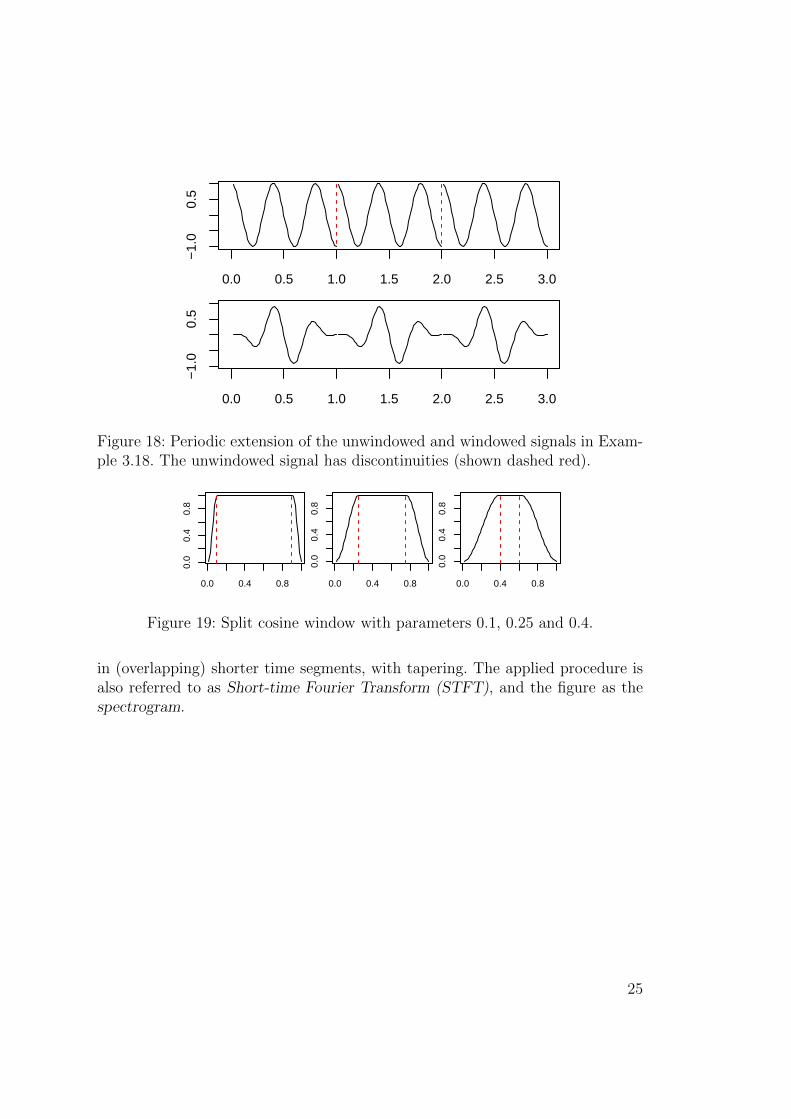
Figure 18: Periodic extension of the unwindowed and windowed signals in Exam-ple 3.18. The unwindowed signal has discontinuities (shown dashed red).

0.0 0.4 0.8

0.0

0.4

0.8

0.0 0.4 0.8

0.0

0.4

0.8

spec

.tape

r(re

p(1,

leng

th(t

)), 0

.25)

0.0 0.4 0.8

0.0

0.4

0.8

spec

.tape

r(re

p(1,

leng

th(t

)), 0

.4)

Figure 19: Split cosine window with parameters 0.1, 0.25 and 0.4.

in (overlapping) shorter time segments, with tapering. The applied procedure isalso referred to as Short-time Fourier Transform (STFT), and the figure as thespectrogram.

25

Time

0.2 0.4 0.6 0.8 1.0

−1.

00.

01.

0

0.0 0.2 0.4 0.6 0.8 1.0

−1.

00.

01.

0

Index

0.0 0.2 0.4 0.6 0.8 1.0

0.5

1.5

2.5

Figure 20: Chirp signal (top), overlapping windowed segments (middle) and the(log-)spectrogram (bottom)

0.0 0.5 1.0 1.5 2.0 2.5

−0.

150.

000.

15

seq(0, T, length = L/7)

0.0 0.5 1.0 1.5 2.0 2.5

1000

4000

Figure 21: Beginning of Suzanne Vega’s Tom’s Diner and spectrogram calculatedwith R specgram (from signal package).

26

4 Box-Jenkins models

Many time-series data cannot be well modelled just by assuming means to followtrends or seasonal variations, and regarding the residual as independent. In manycases, there is an additional layer of correlation between the adjacent time points.We now turn into models which capture dependency structures in the time seriesdata.

Box-Jenkins models9 are fundamental models for stationary processes.When viewed as generative models, they are based on ‘filtering’ of a white noiseprocess. They are all special cases of the following (abstract & theoretical) model.

Definition 4.1 (Linear process). If the process (Xi) can be represented as

Xi = µ+∞∑

j=−∞

cjWi−j,

where µ ∈ R is a common mean, and cj ∈ R are constants with∑

j c2j <∞, and

(Wi) ∼WN(1), then (Xi) is called a (stationary finite variance) linear process.

Definition 4.2 (Causal linear process). The linear process (Xi) is causal, if ithas a representation with cj = 0 for all j < 0.

Remark 4.3. In what follows, we shall concentrate on zero-mean processes. Inpractice, please keep in mind that your data most likely will have a non-zeromean, which may carry important information. . .

4.1 Moving average (MA)

Definition 4.4 (Moving average MA(q)). Suppose θ1, . . . , θq ∈ R are constants,and (Wi) ∼WN(σ2). The MA(q) process with parameters σ2, θ1, . . . , θq is definedas

Xi = Wi + θ1Wi−1 + · · ·+ θqWi−q =

q∑j=0

θjWi−j, (2)

where θ0 = 1 by convention.

Question. Why can we assume θ0 = 1 without loss of generality?

Remark 4.5. Moving average was introduced in Section 2 as a device to smoothany time series data, perhaps for explanatory purposes. The MA(q) can be un-derstood as ‘one-sided’ moving average of a white noise process.

Question. Is ‘two-sided MA(q)’ more general than the ‘one-sided MA(q) above?

Example 4.6. This is a simulation of a specific MA(6) model.

9. These models were largely popularised in statistics following the Box & Jenkins’ influential1976 book Time series analysis, control and forecasting.

27

0 1 2 3 4 5 6

−1.0

0.0

1.0

MA

coe

ffic

ient

0 20 40 60 80 100 120

−4

02

4

Sim

ula

teed

valu

es

0 5 10 15 20

−0.5

0.0

0.5

1.0

AC

F

Figure 22: Simulation of a MA(6) model.

theta <- cos(2*pi*(1:6)/12)

y <- arima.sim(model=list(ma=theta), 133)

# This is the same as:

y <- filter(rnorm(140), c(1,theta), sides=1)[8:140]

Theorem 4.7. The autocovariance of MA(q) can be calculated as follows

γi =

{σ2∑q−|i|

k=0 θkθk+|i|, |i| ≤ q

0, otherwise.

Proof. The MA(q) process has zero mean, so for i ≥ 0

γi = E[X0Xi] = E[( q∑

k=0

θkW−k

)( q∑j=0

θjWi−j

)]

= σ2

q∑k,j=0

θkθjI{k = j − i}

28

= σ2

q∑k=0

θkθk+i,

with the convention θj = 0 for j > q.

Corollary 4.8. The variance and autocorrelation of MA(q) are

Var(Xi) = σ2

q∑k=0

θ2k

ρi =

∑q−|i|

k=0 θkθk+|i|∑qk=0 θ

2k

, |i| ≤ q

0, otherwise

ma_acf <- function(theta) {

# Note that rho[1]=1 (zeroth lag)!

q_1 <- length(theta)

gamma <- convolve(c(1,theta), c(1,theta), type="o")

rho <- gamma[(q_1+1):(2*q_1+1)]/gamma[q_1+1]

}

Definition 4.9 (Backshift operator). Let (Xi) be a stochastic process. The back-shift operator is defined as

BXi := Xi−1 and BjXi := B(Bj−1Xi) = Xi−j for j ≥ 2.

We may write the definition of MA(q) in (2) in terms of the backshiftoperator as follows:

Xi =(

1 +

q∑j=1

θjBj)Wi.

Definition 4.10. The characteristic polynomial of MA(q) is the complex poly-nomial

θ(z) := 1 +

q∑j=1

θjzj.

We may write (2) using the characteristic polynomial as

Xi = θ(B)Wi.

29

4.2 Autoregressive (AR)

Moving average models are causal linear processes by definition. There is anotherclass of models, based on a recursive formulation similar to the exponentiallyweighted moving average.

Definition 4.11 (Autoregressive AR(p)). Suppose φ1, . . . , φp ∈ R are constantsand (Wi) ∼WN(σ2). The AR(p) process with parameters σ2, φ1, . . . , φp is definedthrough

Xi = Wi +

p∑j=1

φjXi−j, (3)

whenever such stationary process (Xi) exists.

Remark 4.12. The process in Definition 4.11 is sometimes called a stationaryAR(p) process. It is possible to consider a ‘non-stationary AR(p) process’ for anyφ1, . . . , φp satisfying (3) for i ≥ 0 by letting for example Xi = 0 for i ∈ [−p+1, 0].

Example 4.13 (Variance and autocorrelation of AR(1) process). For the AR(1)process, whenever it exits, we must have

γ0 = Var(Xi) = Var(φ1Xi−1 +Wi) = φ21γ0 + σ2,

which implies that we must have |φ1| < 1, and

γ0 =σ2

1− φ21

.

We may also calculate for j ≥ 1

γj = E[XiXi−j] = E[(φ1Xi−1 +Wi)Xi−j] = φ1E[Xi−1Xi−j] = φj1γ0,

which gives that ρj = φj1.

Example 4.14. Simulation of an AR(1) process.

phi_1 <- 0.7

x <- arima.sim(model=list(ar=phi_1), 140)

# This is the explicit simulation:

gamma_0 <- 1/(1-phi_1^2)

x_0 <- rnorm(1)*sqrt(gamma_0)

x <- filter(rnorm(140), phi_1, method = "r", init = x_0)

Example 4.15. Consider a stationary AR(1) process. We may write

Xi = φ1Xi−1 +Wi = · · · = φn1Xi−n +n−1∑j=0

φj1Wi−j.

30

Sim

ula

ted v

alu

es

0 20 40 60 80 100 120 140

−4

02

4

0 5 10 15

−0

.20.2

0.6

1.0

AC

F

Figure 23: Simulation of AR(1) process in Example 4.14.

0 5 10 15

0.0

0.4

0.8

phi_1 = 0.9

0 5 10 15

−0.5

0.5

phi_1 = −0.9

0 5 10 15

0.0

0.4

0.8

phi_1 = 0.5

0 5 10 15

−0.5

0.5

phi_1 = −0.7

Figure 24: Autocorrelations of AR(1) with different parameters.

31

Define the causal linear process Yi =∑∞

j=0 φj1Wi−j, then we may write (detailed

proof not examinable)

(E|Xi − Yi|2

)1/2=

(E∣∣∣φn1Xi−n −

∞∑j=n

φj1Wi−j

∣∣∣2)1/2

≤ |φ1|n(EX2

i−n)1/2

+∞∑j=n

|φ1|j(EW 2

i−j)1/2

= |φ1|n(σX +

σ

1− |φ1|

)n→∞−−−→ 0,

where σ2X = EX2

1 . This implies Xi = Yi (almost surely).

We may write the autoregressive process also in terms of the backshiftoperator, as

Xi −p∑j=1

φjBjXi = Wi, (4)

or φ(B)Xi = Wi, where

Definition 4.16 (Characteristic polynomial of AR(p)).

φ(z) := 1−p∑j=1

φjzj.

Remark 4.17. Note the minus sign in the AR polynomial, contrary to the plus inthe MA polynomial. In some contexts (esp. signal processing), the AR coefficientsare often defined φi = −φi, so that the AR polynomial will look exactly like theMA polynomial.

Theorem 4.18. The (stationary) AR(p) process exists and can be written as acausal linear process if and only if

φ(z) 6= 0 for all z ∈ C with |z| ≤ 1,

that is, the roots of the complex polynomial φ(z) lie strictly outside the unit disc.

For full proof, see for example Theorem 3.1.1 of Brockwell and Davis.However, to get the idea, we may write informally

Xi = φ(B)−1Wi,

and we may write the reciprocal of the characteristic function as

1

φ(z)=∞∑j=0

cjzj, for |z| ≤ 1 + ε,

32

This means that we may write the AR(p) as a causal linear process

Xi =∞∑j=0

cjWi−j,

where the coefficients satisfy10 |cj| ≤ K(1 + ε/2)−j.

Remark 4.19. This justifies viewing AR(p) as a ‘MA(∞)’ with coefficients (cj)j≥1.This also implies that we may apporximate AR(p) with ‘arbitrary precision’ byMA(q) with large enough q.

4.3 Invertibility of MA

Example 4.20. Let θ1 ∈ (0, 1) and σ2 > 0 be some parameters, and consider twoMA(1) models,

Xi = Wi + θ1Wi−1, (Wn)i.i.d.∼ N(0, σ2)

Xi = Wi + θ1Wi−1, (Wn)i.i.d.∼ N(0, σ2),

where θ1 = 1/θ1 and σ2 = σ2θ21. We have

γ0 = σ2(1 + θ21), γ1 = σ2θ1

γ0 = σ2(1 + θ21) γ1 = σ2θ1.

What do you observe?

It turns out that the following invertibility condition resolves the MA(q)identifiability problem, and therefore it is standard that the roots of the charac-teristic polynomial are assumed to lie outside the unit disc.

Theorem 4.21. If the roots of the characteristic polynomial of MA(q) are strictlyoutside the unit circle, the MA(q) is invertible in the sense that it satisfies

Wi =∞∑j=0

βjXi−j,

where the constants satisfy β0 = 1 and |βj| ≤ K(1 + ε)−j for some constantsK <∞ and ε > 0.

As with Theorem 4.18, we may write symbolically, from Xi = θ(B)Wi,that

Wi =1

θ(B)Xi =

∞∑j=0

βjXi−j,

where the constants βj are uniquely determined by 1/θ(z) =∑∞

j=0 βjzj, as the

roots of θ(z) lie outside the unit disc.

10. Because∑cj(1 + ε/2)j → 0 as j →∞.

33

4.4 Autoregressive moving average (ARMA)

Definition 4.22 (Autoregressive moving average ARMA(p,q) process). Supposeφ1, . . . , φp ∈ R are coefficients of a (stationary) AR(p) process and θ1, . . . , θq ∈ R,and (Wi) ∼WN(σ2). The (stationary) ARMA(p,q) process with these parametersis a process satisfying

Xi =

p∑j=1

φjXi−j +

q∑j=0

θjWi−j, (5)

with the convention θ0 = 1 and where the first sum vanishes if p = 0.

Remark 4.23. AR(p) is ARMA(p,0) and MA(q) is ARMA(0,q).

We may write ARMA(p,q) briefly with the characteristic polynomials ofthe AR and MA and the backshift operator as

φ(B)Xi = θ(B)Wi.

Simulation of a general ARMA(p,q) model is not straightforward exactly,but we can approximately simulate it by setting X−p+1 = · · · = X0 = 0 (say)and then following (5). Then, Xb, Xb+1, . . . , Xb+n is an approximate sample of astationary ARMA(p,q) if b is ‘large enough’. This is what R function arima.sim

does; the parameter n.start is b above.

Example 4.24. Simulation of ARMA(2,1) model with φ1 = 0.3, φ2 = −0.4, θ1 =−0.8.

x <- arima.sim(list(ma = c(-0.8), ar=c(.3,-.4)),

140, n.start = 1e5)

This is the same as

q <- 2; n <- 140; n.start <- 1e5

z <- filter(rnorm(n.start+n), c(1, -0.8), sides=1)

z <- tail(z, n.start+n-q)

x <- tail(filter(z, c(.3,-.4), method="r"), n)

(The latter may sometimes be necessary, because arima.sim checks the stabilityof the AR part by calculating the roots of φ(z) numerically, which is notoriouslyunstable if the order of φ is large. Sometimes arima.sim refuses to simulate astable ARMA. . . )

Remark 4.25. If the characteristic polynomials θ(z) and φ(z) of an ARMA(p,q)share a (complex) root, say x1 = y1, then

θ(z)

φ(z)=cθ(z − x1)(z − x2) · · · (z − xq)cφ(z − y1)(z − y2) · · · (z − yp)

34

Sim

ula

teed v

alu

es

0 20 40 60 80 100 120 140

−4

−2

02

0 5 10 15

−0.5

0.5

1.0

AC

F

Figure 25: Simulation of ARMA(2,1) in Example 10.6.

=cθ(z − x2) · · · (z − xq)cφ(z − y2) · · · (z − yp)

=θ(z)

φ(z),

where θ(z) is of order q − 1 and φ(z) is of order p− 1, and it turns out that

φ(B)Xi = θ(B)Wi,

which means that the model reduces to ARMA(p− 1,q − 1).

Condition 4.26 (Regularity conditions for ARMA). In what follows, we shallassume the following:

(a) The roots of the AR characteristic polynomial are strictly outside the unitdisc (cf Theorem 4.18).

(b) The roots of the MA characteristic polynomial are strictly outside the unitdisc (cf. Theorem 4.21).

(c) The AR and MA characteristic polynomials do not have common roots(cf. Remark 4.25).

35

Theorem 4.27. A stationary ARMA(p,q) model satisfying Condition 4.26 ex-ists, is invertible and can be written as a causal linear process

Xi =∞∑j=0

ξjWi−j, Wi =∞∑j=0

βjXi−j,

where the constants ξj and βj satisfy

∞∑j=0

ξjzj =

θ(z)

φ(z)and

∞∑j=0

βjzj =

φ(z)

θ(z).

In addition, β0 = 1 and there exist constants K < ∞ and ε > 0 such thatmax{|ξj|, |βj|} ≤ K(1 + ε)−j for all j ≥ 0.

Remark 4.28. In fact, the coefficients ξj (or βj) related to any ARMA(p,q) can becalculated numerically from the parameters easily. Also the autocovariance canbe calculated numerically up to any lag in a straightforward way; cf. Brockwelland Davis p. 91–95. In R, the autocorrelation coefficients can be calculated withARMAacf.

4.5 Integrated models

Autoregressive moving average models are pretty flexible models for stationaryseries. However, in many practical time series, it might be more useful to considerthe differenced series (Definition 2.10). This brings us to the general notion of

Definition 4.29 (Difference operator). Suppose (Xi) is a stochastic process. Itsd:th order difference process is defined as (∇dXi), where the d:th order differenceoperator may be written in terms of the backshift operator as ∇d = (1−B)d ford ≥ 1.

Definition 4.30 (Autoregressive integrated moving average ARIMA(p,d,q) pro-cess). If the d-th difference of the process (∇dXi) follows ARMA(p,q), then wesay (Xi) is ARIMA(p,d,q).

Remark 4.31. Suppose that (∇dXi) is a stationary ARMA(p, q).(i) The ARIMA(p,d,q) process (Xi) is not unique (why?).(ii) The ARIMA(p,d,q) process (Xi) is not, in general, stationary.

The process (Xi) (or the data x1, . . . , xn) is said to be difference stationary.

Example 4.32. Simple random walk

Xi = Xi−1 +Wi

is an ARIMA(0,1,0).

36

Sim

ula

teed

va

lue

s

0 20 40 60 80 100 120 140

−6

−2

2

0 5 10 15

−0

.20.2

0.6

1.0

AC

F

0 5 10 15

−0.5

0.5

1.0

AC

F

Figure 26: Simulation of ARIMA(1,1,0) in Example 4.33. The first ACF is for thesimulated series, and the second is the ACF of the differences.

Example 4.33. Simulation of ARIMA(1,1,0) model with φ1 = −0.5.

x <- arima.sim(list(order=c(1,1,0), ar=c(-.5)),

140, n.start = 1e5)

If the random walk is considered as a ‘non-stationary AR(1)’, then it’scharacteristic polynomial is φ(z) = 1 − z, with unit root z = 1. We have, ingeneral, the following:

Proposition 4.34. Suppose that φ(B)Xt = θ(B)Wt and the characteristicpolynomial of φ(z) = 1 −

∑pj=1 φjz

j has unit root, that is, φ(1) = 0. Then,

φ(B)(∇Xt) = θ(B)Wt for certain characteristic polynomial φ(B) of order p− 1.

Proof. If φ(1) = 0, then

φ(z) = c(z − 1)

p∏j=2

(z − rj) = φ(z)(1− z),

37

for some c ∈ R \ {0} and roots rj ∈ C. Therefore,

φ(B)(1−B)Xt = φ(B)(∇Xt) = θ(B)Wt.

Question. What does it mean if φ(B)Xt = θ(B)Wt and φ(z) has a unit root withmultipllicity d?

Remark 4.35. There are unit root tests for detecting non-stationarity. (The nullis the existence of a unit root, that is, non-stationarity.)

4.6 Seasonal dependence

Seasonal behaviour is often modelled conveniently by considering explicitly theseasonal dependence in the ARMA or ARIMA models.

Definition 4.36. Purely seasonal ARMA(P ,Q)s with season s > 1 is a processwhich follows

Xi =P∑j=1

ϕjXi−js +

Q∑j=0

ϑjWi−js, (6)

where ϑ0 = 1.Let ϕ(z) = 1−

∑Pj=1 ϕjz

j and ϑ(z) = 1 +∑Q

j=1 ϑjzj be the characteristic

polynomials of the seasonal AR and MA parts, respectively, then we may write(6) concisely as

ϕ(Bs)Xi = ϑ(Bs)Wi.

Question. Can you write seasonal ARMA(P ,Q)s as ARMA(p,q) for some p andq?What does that mean in terms of regularity conditions required for ϕ(zs) andϑ(zs)?

It is rare that a purely seasonal model is appropriate, as there are oftenalso correlation between adjacent values. The common way is to combine boththe seasonal and the non-sesaonal models.

Definition 4.37. Autoregressive moving average model with seasonal elementARMA(p,q)(P ,Q)s with season s > 1 is a process (Xi) which follows

ϕ(Bs)φ(B)Xi = ϑ(Bs)θ(B)Wi,

where φ and ϕ are AR characteristic polynomials with orders p and P , and like-wise θ and ϑ are MA characteristic polynomials with orders q and Q, respectively.

Remark 4.38. Note again that ARMA(p,q)(P ,Q)s is just ARMA(Ps+ p,Qs+ q)with certain parameterisation of the coefficients, and often some coefficients setto zero. Again, all ϕ(zs), φ(z), ϑ(zs) and θ(z) are assumed to have all zeroesstrictly outside the unit disc, and ϕ(zs)φ(z) not sharing roots with ϑ(zs)θ(z).

38

0 5 10 15 20 25

0.0

0.4

Jo

int M

A c

oe

ffs

Sim

ula

teed

valu

es

0 20 40 60 80 100 120 140

−4

02

4

0 5 10 15 20 25

−0.2

0.2

0.6

1.0

AC

F

Figure 27: Simulation of Example 4.39.

Example 4.39. Simulation of ARMA(0,2)(0,2)12 with ϑ1 = 0.75 = θ1 and ϑ2 =0.5 = θ2.

s <- 12; p <- 2; P <- 2; n.sim <- 140

theta <- c(0.75, 0.5); theta_s <- theta

theta_s_ <- rep(0,P*s)

theta_s_[seq(from=s, to=P*s, by=s)] <- theta_s

theta_joint <- convolve(c(1,theta_s_), rev(c(1,theta)),

type="o")[2:(P*s+p+1)]

x <- arima.sim(list(ma = theta_joint), n.sim)

Finally, we may put everything together, yielding a ‘ARIMA with seasonalcomponents’, sometimes dubbed ‘SARIMA’.

Definition 4.40. ARIMA(p,d,q)(P ,D,Q)s with season s > 1 is a process (Xi)which follows

ϕ(Bs)φ(B)∇Ds ∇dXi = ϑ(Bs)θ(B)Wi,

39

0 50 100 150

−2

50

−10

00

Sim

ula

ted

va

lue

s

0 5 10 15 20 25

−0

.20

.20

.61

.0

Sam

ple

AC

F

0 5 10 15 20 25

−0.2

0.2

0.6

1.0

Diffe

renced A

CF

Figure 28: Simulation of Example 4.41.

where φ and ϕ are AR characteristic polynomials with orders p and P , and like-wise θ and ϑ are MA characteristic polynomials with orders q and Q, respectively.

In applications, it is common that many of p, d, q, P,D,Q are set to zero,leading into a simpler form. However, the general form is good to recognise, forinstance because the R function arima estimates parameters for any such model.

Example 4.41. Consider the ARIMA(0,1,2)(0,1,2)12 with θ1 = 0.75 = ϑ1, θ2 =0.5 = ϑ2, and assume theta_joint is defined as in Example 4.39.

s <- 12; n.sim <- 140

y <- arima.sim(list(ma = theta_joint), n.sim)

x <- diffinv(diffinv(y), lag=s)

# This is what happens above:

z <- cumsum(y); y_ <- rep(0, n.sim)

for (k in 1:s) {

y_[seq(k, n.sim, by=s)] <- cumsum(z[seq(k, n.sim, by=s)])

}

40

5 Parameter estimation

We now turn into estimation of parameters of ARIMA models, which can be donein R using the function arima.

5.1 Mean and trends

In Section 4, we considered only zero-mean models. In practice, the series willoften have a non-zero mean. In practice, we need to set xi = xi−µ and regard (xi)as a realisation of an ARIMA(p,d,q) process (Xi), and estimate simultaneouslyboth µ and the ARMA parameters φ1, . . . , φp, θ1, . . . , θq, σ

2.More generally, it is often useful to regress (xi) first, in terms of some

regressors (z(j)i ), such that

xi = xi −m∑j=1

β(j)z(j)i , and (xi) ∼ (Xi)

where β(1), . . . , β(n) ∈ R are estimated together with the parameters of theARIMA(p,d,q)(P ,D,Q)s. We do not discuss this in more detail, but we applythis in practice.

Remark 5.1. R allows to add external regressors to the model. Please note thatin R, when fitting ARMA models with arima, the mean µ is estimated and theARMA is fitted to xi = xi − µ. However, when fitting ARIMA models, withdifferencing, the mean µ is assumed zero.

# X_t = W_t + k*50

x <- rnorm(140)+(1:140)*50

m1 <- arima(diff(x), order=c(0,0,1)) # automatic intercept

m2 <- arima(x, order=c(0,1,1)) # no intercept -> wrong model

m3 <- arima(x, order=c(0,1,1), xreg=1:140) # equivalent to m1

Here m1 and m3 are the same model! Note that the external regressor regressesthe original series, not the differenced one, in m3.

5.2 Autoregressive model

We start by considering parameter estimation for the AR(p) model in a bit moredetail.

Theorem 5.2 (Yule-Walker equations). The autocovariance function of anAR(p) satisfies the equations

γ = Γφ (7)

γ0 = σ2 + γTφ, (8)

where γ = (γ1, . . . , γp)T , [Γ]ij = γ|i−j| and φ = (φ1, . . . , φp)

T .

41

Proof. We may assume, without loss of generality, a zero mean AR(p) process(Xi), for which by definition

XiXi−k = WiXi−k +

p∑j=1

φjXi−jXi−k.

For k ≥ 0, taking expectations leads to

γk = σ2I{k = 0}+

p∑j=1

φjγ|j−k|.

We obtain (8) from k = 0 and (7) from k = 1, . . . , p.

The Yule-Walker equations suggest a simple method for estimating theparameters φ1, . . . , φp.

Definition 5.3 (Yule-Walker estimates). The YW estimates of φ1, . . . , φp andσ2 are calculated as follows:

(i) Calculate γk for k = 0, . . . , p (and also µ = x).

(ii) Solve φ from γ = Γφ.

(iii) Solve σ2 from γ0 = σ2 + γT φ.

Remark 5.4. If γ0 > 0, the matrix Γ is invertible (because positive definite!), andtherefore the Yule-Walker estimates φ are unique. Note that dividing by γ0, theestimates can be written in an alternative form

φ = R−1ρ and σ2 = γ0(1− ρT R−1ρ),

where ρ = (ρ1, . . . , ρp) and [R]ij = ρ|i−j|. In addition, if γ0 > 0, the estimates φdefine a stationary AR model.

Remark 5.5. Solving φ directly by matrix inversion would involve O(p3) opera-tions. Because of the specific structure11, the coefficients can be solved (even more)efficiently using only O(p2) operations. The standard method is the Levinson-Durbin algorithm. The Levinson-Durbin algorithm is particularly convenient be-cause it computes recursively the coefficients φ and variance estimates σ2 forall intermediate models, that is, AR(1), AR(2), . . . , and AR(p). This is veryconvenient in model selection.

The Yule-Walker estimates are consistent, and satisfy a central limit the-orem.

11. The matrix Γ is Toeplitz: all the diagonals of Γ are equal.

42

Ori

gin

al

0 500 1000 1500 2000

−0.4

0.0

0.4

0 50 100 150 200

−0.5

0.0

0.5

1.0

AC

F

Re

sid

ual

0 500 1000 1500 2000

−0.0

50.0

5

0 50 100 150 200

0.0

0.4

0.8

AC

F

Genera

ted

0 500 1000 1500 2000

−0.4

0.0

0.4

0 50 100 150 200

−0.5

0.0

0.5

1.0

AC

F

Figure 29: AR model fit into speech sample “ah” (top), the residual, and therandom sample of the model (bottom).

Theorem 5.6. If (Xi) is stationary AR(p) with (Wi) ∼WN(σ2), and φ(n)

is theYW estimates based on X1, . . . , Xn, then

√n(φ

(n)− φ)

n→∞−−−→ N(0, σ2Γ−1), in distribution.

Moreover, σ2 → σ2 in probability.

For proof, see Brockwell and Davis, Theorem 8.1.1.

Example 5.7. The mobile phone (GSM) standard involves lossy speech compres-sion based on “linear prediction coefficients”, which is engineering terminology“AR coefficients”. Figure 29 shows a the beginning of a 0.5 second speech sampleof “ah” at 8000 samples per second, the corresponding residual of AR(100) fit tothe sample, and a random sample of AR(100).

(The compression includes both the AR coefficients and an additionalresidual compression, which involves a lot of fine tuning. . . )

In the AR model, we have

(Xi − µ)−p∑j=1

φj(Xi−j − µ) = Wi,

43

and we could think also the following estimator

Definition 5.8 (Conditional sum of squares). The conditional sum of squares,or conditional least squares estimator of φ = φ1, . . . , φn and µ is

(φ, µ) := arg min(φ,µ)

Sc(x1, . . . , xn;φ, µ),

Sc(x1, . . . , xn;φ, µ) :=n∑

i=p+1

(xi − µ−

p∑j=1

φj(xi−j − µ))2. (9)

If we differentiate wrt. µ and set to zero, we get

µ =

∑ni=p+1(xi −

∑pj=1 φjxi−j)

(n− p)(1−∑p

j=1 φj)=

1

n− p

( n−p∑i=p+1

xi +Rn,p

)≈ x,

if n is large, because Rn,p is a residual term of order O(p2). If we substitute µ = x

in (9) and differentiate wrt. φk and set to zero, we get that the estimates φjshould satisfy

1

n

n∑i=p+1

(xi−k − x)(xi − x)−p∑j=1

φj

(1

n

n∑i=p+1

(xi−k − x)(xi−j − x)

)= 0,

which is, for large n, close to

γk =

p∑j=1

φj γ|j−k|,

which corresponds to the Yule-Walker estimate. This shows that for large n, theYule-Walker estimates are going to be similar to the CSS estimates.

Example 5.9. Assume next an AR(1) with Gaussian white noise (Wn)i.i.d.∼

N(0, σ2). We can write the likelihood now as

`(x1, . . . , xn) = N

(x1 − µ; 0,

σ2

1− φ21

) n∏i=2

N(xi − µ;φ1(xi−1 − µ), σ2

),

where N(x,m, σ2) stands for the Gaussian p.d.f. Denoting xi = xi − µ, we canexpand

log ` = −1− φ21

2σ2x21 −

1

2σ2

n∑i=2

(xi − φ1xi−1)2 − n

2log σ2 +

1

2log(1− φ2

1) + c

= − 1

2σ2Sc(x1, . . . , xn;φ1, µ) +R1(x1, σ

2, φ21, µ).

44

As the number of samples increases, the conditional sum of squares term willdominate, meaning that the maximum likelihood estimator will be similar to theCSS, and hence the YW estimators.

Remark 5.10. Finding both the CSS and the ML estimates requires, in general,iterative numerical optimisation methods.

The story about the maximum likelihood estimates of a general AR(p)is similar: The first p variables follow a multivariate Gaussian distribution, andthe conditional sum of squares term will be the dominating one, so the maximumlikelihood estimates will coincide with the YW and CSS estimates asymptotically.Keep in mind, however, that with any finite n, the Yule-Walker, the CSS and theML estimates will all be generally different, and may be preferable in specificapplications. The R arima used ML by default.

Question. Can you give some reasons why each of the three variants could beuseful in certain applications?

5.3 General ARMA

We saw earlier that the Yule-Walker method of estimation for the AR modelswas straightforward and efficient, and coincides asymptotically with the CSS andthe ML estimators. There are not as simple and well-behaved methods for theestimation of parameters in the general ARMA model, and one has to resort tonumerical optimisation.

If the time series is not too long, and if the fitted model does not havetoo many parameters, it is common to use maximum likelihood estimation inthe ARIMA context, assuming Gaussian white noise. This is also what the Rstandard ARIMA fitting tool arima does.

The ML estimation requires iterative numerical optimisation methods, andwe shall not take a closer look at the methods now. Instead, we quote the followingasymptotic normality result.

Theorem 5.11. (not examinable) Suppose β = (φ,θ) are parameters of anARMA(p,q) process (Xi) with Gaussian (Wi) ∼ WN(σ2), which satisfies Con-

dition 4.26. Let β(n)

= (φ(n), θ

(n)) stand for the ML estimator calculated from

(X1, . . . , Xn), then,

√n(β

(n)− β)

n→∞−−−→ N(0, V (β)

), in distribution,

where the covariance matrix V (β) can be expressed as

V (β) = σ2

[EUUT EUV T

EV UT EV V T

]−1,

U = (Up, . . . , U1)V = (Vq, . . . , V1),

45

where (Ui) and (Vi) are AR(p) and AR(q) processes satisfying

φ(B)Ui = Wi and θ(B)Vi = Wi.

In case of p = 0 or q = 0, the corresponding matrices vanish.

See Brockwell and Davis, Section 8.8. We note that the confidence intervalsof the estimated parameters may be (and are) calculated from the Hessian,

1

nV (β) ≈

([− ∂2

∂βi∂βj`(β)

]i,j

)−1,

where ` is the log-likelihood of β.

6 Model selection tools

Perhaps the most challenging question in time series analysis is to find a satis-factory model class. In the case of real data, there rarely is a correct model, andwhat is satisfacotry depends on what the model is used for. We will next looksome tools which may indicate which models might be appropriate.

The first thing to do is always to inspect the data. Plot the time series, orif it is long, look for shorter segments of the data at the time. Look for obvioustrends or other behaviour suggesting non-stationary. Inspect also cyclic or near-cyclic behaviour. Autocorrelation plots and the periodogram can be helpful, theycan also suggest cyclic components. Remember to try also transformations, suchas log-transform or Box-Cox transforms.

It can be instructive to look at the data agains lagged versions of itself,that is, the scatterplots of (Xi, Xi+k).

Example 6.1. Lag plots of the speech data in Example 5.7.

lag.plot(x, layout=c(2,3), set.lags=c(1:3, 32, 72, 104),

pch=".")

6.1 Non-stationarity

If the data shows signs of non-stationarity, recall that you may inspect the differ-ences. Note, however, that if removal of a trend makes the data seem stationary(data is trend stationary), it is possible to consider the original data with anexternal regressor handling the trend.

Remark 6.2. Unit root tests were mentioned in Section 4.5. We shall not discussunit root tests further, but only note that there are some implemented in Rlibrary tseries: the Augmented Dickey-Fuller test adf.test and the Phillips-Perron test pp.test.

46

lag 1

x

−0

.40

.00.2

0.4

−0.4 0.0 0.2 0.4

lag 2x

lag 3

x

−0.4 0.0 0.2 0.4

lag 32

x

lag 72

x

−0.4 0.0 0.2 0.4

lag 104

x

−0.4

0.0

0.2

0.4

Figure 30: Lag plots of the speech data in Example 5.7.

6.2 Autocorrelation

Theorem 1.17 stated asymptotic normality of the sample ACF in case of whitenoise. The following generalises that for a large class of linear processes.

Theorem 6.3. (Not examinable) Suppose (Xi) is a stationary process given by

Xi = µ+∞∑

j=−∞

cjWj, (Wi) ∼WN(σ2),

with coefficients satisfying∑

j |cj| < ∞ and∑

j |j|c2j < ∞, and let (ρk) be itsautocorrelation.

Then, for any h ∈ N, the sample autocorrelations ρ(n)k calculated from

X1, . . . , Xn satisfy

√n(ρ(n)1 − ρ1, . . . , ρ

(n)h − ρh

) n→∞−−−→ N(0,Wh) in distribution,

where the limiting covariance matrix is given as

[Wh]ij =∞∑k=1

(ρk+i − ρk−i − 2ρiρk

)(ρk+j − ρk−j − 2ρjρk

)For a proof, see Brockwell and Davis Theorem 7.2.2.

Remark 6.4. Theorem 6.3 justifies us to say that (ρ1, . . . , ρh) is approximatelyN((ρ1, . . . , ρh),Wh/n

)for large n. Note that Theorem 6.3 holds for any stationary

47

ARMA(p,q), because we know that it has representation with cj = 0 for j < 0and |cj| decay exponentially in j.

Corollary 6.5. Suppose (Xi) is a MA(q). Then, for all i > q,

√n(ρi − ρi)→ N(0, σ2

i ),

where

σ2i = 1 + 2

q∑j=1

ρ2j .

Proof. Left aso an exercise.

The result of Corollary 6.5 is used by R acf, when called withci.type="ma". It displays confidence bounds based on

σ2k = 1 + 2

k−1∑j=1

ρ2j .

Question. Can you explain what is the rationale of this? What about the possiblecaveats?

Example 6.6. Comparison of ACF with standard and MA confidence bounds.

x = arima.sim(model=list(ma=c(3/4, -1/5, -1/5)), 100)

par(mfrow=c(2, 1))

acf(x); acf(x, ci.type="ma")

6.3 Partial autocorrelation function

Definition 6.7. The partial autocorrelation function (PACF) (αk)k≥0 of a zero-mean finite variance stationary process (Xi) is defined as ρ0 = 1 = α0 andρ1 = α1, and for k ≥ 2 through

αk = Corr(Xk+1 − Xk+1|2:k, X1 − X1|2:k),

where Xk+1|2:k and X1|2:k are the best linear predictors (in the mean squaresense)12, of Xk+1 and X1 given X2, . . . , Xk, respectively.

Theorem 6.8. The partial autocorrelation of AR(p) process αk = 0 for all k > p.

12. Recall that the best linear predictor X of a random variable X given Y1, . . . , Yn in themean square sense is X =

∑nj=1 cjYj , where the constants (c1, . . . , cn) are chosen to minimise

E[(X −X)2]. That is, the partial autocorrelation is correlation of the residuals of Xk+1 and X1

after regressing with X2, . . . , Xk.

48

0 5 10 15 20

−0.2

0.4

1.0

0 5 10 15 20

−0.2

0.4

1.0

Proof. Let k > p, then we have

E[Xk+1 | X2, . . . , Xk] = E[ p∑j=1

φjXk+1−j +Wk+1

∣∣∣∣ X2, . . . , Xk

]

=

p∑j=1

φjXk+1−j,

because Wk+1 is independent of X2, . . . , Xk and 2 ≤ k + 1 − j ≤ k in the sum.Because conditional expectation minimises the mean square error, we deduce that(in this specific case!) Xk+1|2:k =

∑pj=1 φjXk+1−j. We then conclude,

αk = Corr(Wk+1, X1 − X1|2:k) = 0.

Theorem 6.9. Let ρk be the autocorrelation of a stationary process (Xi), and

assume β(k) = (β(k)1 , . . . , β

(k)k ) is the solution of

R(k)β(k) = ρ(k), where ρ(k) = (ρ1, . . . , ρk) and [R(k)]ij = ρ|i−j| for 1 ≤ i, j ≤ k.

Then, the partial autocorrelation αk = β(k)k for k ≥ 2.

The proof can be found, for example, from Brockwell and Davis, Corollary5.2.1.

Definition 6.10. The sample PACF αk = β(k)k , where β

(k)satisfies R(k)β

(k)=

ρ(k), with R(k) and ρ(k) standing for the R(k) and ρ(k) with the autocorrelationsreplaced with their corresponding sample quantities.

49

Remark 6.11. The partial autocorrelations can be calculated iteratively with theLevinson-Durbin algorithm, as discussed in Section 5.2. Note that each αp cor-

responds to the last estimated autocorrelation coefficient φp of the AR(p) Yule-Walker estimates.

Example 6.12. (Not examinable) The PACF of MA(1) is (exercise)

αk = −(−θ1)k(1− θ21)1− θ2(k+1)

1

.

The general story is similar (and very much examinable!): For MA(q), thePACF will not vanish but will tail off, just like the ACF for AR(p).

Theorem 6.13. Assume (Xi) is AR(p), then the partial autocorrelation coeffi-

cient α(n)k calculated from X1, . . . , Xn satisfies

√nα

(n)k

n→∞−−−→ N(0, 1),

for k > p.

This follows from from asymptotic of Yule-Walker estimates stated in The-orem 5.6 (cf. Brockwell and Davis Ex. 8.15). It is the basis of the PACF confidenceintervals in R.

Example 6.14. Figure 6.14 shows ACF and PACF of simulated AR(1) with φ1 =3/4, MA(1) with θ1 = 3/4 and random walk.

n = 300

x.ar <- arima.sim(model=list(ar=c(3/4)), n)

x.ma <- arima.sim(model=list(ma=c(3/4)), n)

x.rw <- cumsum(rnorm(n))

par(mfrow=c(3,3))

ts.plot(x.ar); acf(x.ar); pacf(x.ar)

ts.plot(x.ma); acf(x.ma); pacf(x.ma)

ts.plot(x.rw); acf(x.rw); pacf(x.rw)

6.4 Information criteria

Autocorrelation and partial autocorrelation plots can suggest certain low-orderAR and MA models, respectively. For a mixed ARMA(p,q) with p > 1 andq > 1, neither ACF or PACF vanish, providing little help. Further, comparingAR, ARMA and MA models can be very difficult, because the model families arenot ordered (how to compare AR(2) and ARMA(1, 1), say?).

It is possible (and quite popular) to base model choice based on genericinformation criteria such as Akaike’s AIC, AIC with correction AICc, and the

50

0 50 150 250

−4

02

0 5 10 15 20

0.0

0.4

0.8

5 10 15 20

0.0

0.4

0.8

0 50 150 250

−3

−1

13

0 5 10 15 20

0.0

0.4

0.8

5 10 15 20

−0.2

0.2

0 50 150 250

−15

−10

−5

0

0 5 10 15 20

0.0

0.4

0.8

5 10 15 20

0.0

0.4

0.8

Figure 31: Data (left), ACF (middle) and PACF (right) of AR(1) (top), MA(1)(middle) and random walk (bottom) of Example 6.14.

Bayesian BIC:

AIC := −2 ln `ML + 2k

AICc := −2 ln `ML +2kn

n− k − 1= AIC− 2k(k + 1)

n− k − 1

BIC := −2 ln `ML + k lnn,

where n is the length of the data, `ML is the likelihood of the ML estimate andk = p+ q + 2 is the number of parameters (including mean and variance).

Remark 6.15. Note that AICc converges to AIC as n tends to infinity, but thepenalty of BIC will be higher, leading to favour models with less parameters.

fit <- arima(x, order=c(p,0,q))

n <- length(x); k <- q+p+2

fit.aic <- AIC(fit)

fit.aicc <- AIC(fit, k=2*n/(n-k-1))

fit.bic <- AIC(fit, k=log(n))

There is even an automatic ARIMA model fitting tool in R, which searchesfor the best (low order) ARIMA in terms of some of the information criteria.

51

library(forecast)

log_AP <- log(AirPassengers)

fit <- auto.arima(log_AP, ic="aicc")

7 Model diagnostics

The model diagnostics final step in the three-step procedure for time series modelbuilding suggested by (and attributed to) the Box and Jenkins (1970):Identification where we look at the data (with ACF, PACF, differencing, lag

plots, periodogram. . . ), and also any subject-specific information aboutthe data, to suggest subclasses of parsimonious models we might consider.

Estimation where we fit the chosen model, or models of interest, to the data.Diagnostic checking where we study how the model fits the data, and look for

any signs of an inadequate fit using formal hypothesis tests.The steps overlap, as is the case with information criteria which can only be foundafter estimation of the parameters. Please bear in mind that this procedure wassuggested when computing was expensive, and even then the procedure was meantto be iterative; the most adequate model may not be found in one iteration.

7.1 Residuals

Let us next take a closer look at the residuals of the ARMA models. Notice thatin the time series context, there is no natural decomposition of the data to ‘fittedvalues’ and ‘the residuals’. Please keep this mind when using the R functionsfitted and resid with time series models; see Figure 32.

Consider first an AR(p). If the data is really from AR(p), and if the esti-mated parameters are close to their true values, we should have the residuals

ei = (xi − µ)−p∑j=1

φj(xi−j − µ), i = p+ 1, . . . , n

distributed approximately according to white noise.Likewise, for general ARMA(p,q), the residuals can be expressed as

ei = xi − E[Xi | X1 = x1, . . . , Xi−1 = xi−1],

where the conditional expectation is with respect to the process (Xi) followingthe ARMA with the estimated parameters (φ, θ, σ2, µ).

The first step in the residual analysis is to look at the ACF and PACF ofthe residuals, whether they appear similar to those calculated from white noise.

52

5 10 15 20

46

810

5 10 15 20

−3

−1

1

Figure 32: Residuals of a linear model (top) and residuals of an AR(1) withφ1 = 3/4 (bottom).

7.2 Residual tests

Definition 7.1 (Box-Pierce test). The Box-Pierce statistic is calculated for somep+ q < K � n,

Q = nK∑j=1

r2j ,

where rj is the sample autocorrelation of the residual series. If the model is correct,then Q is approximately distributed as χ2

K−p−q.13

Definition 7.2 (Ljung-Box test). The Ljung-Box test is exactly as Box-Pierce,but with a modified statistic

Q = nK∑j=1

n+ 2

n− jr2j ,

which has been found empirically to be often a more accurate approximation ofχ2K−p−q.

Example 7.3. Ljung-Box with MA(3) fitted to simulated AR(2).

13. That is, the null (that the model is correct) is rejected if Q is greater than the 1−α quantileof χ2

K−p−q.

53

Standardized Residuals

0 20 40 60 80

−2

02

0 5 10 15

−0

.20.4

1.0

2 4 6 8 10

0.0

0.4

0.8

p values for Ljung−Box statistic

Figure 33: You should not trust the Ljung-Box statistic reported by R functiontsdiag(fit). . .

n <- 80; q <- 3; p <- 0

x <- arima.sim(model=list(ar=c(1/2, 1/3)), n)

fit <- arima(x, order=c(p,0,q));

e <- resid(fit); pval <- rep(NA,10)

for(lag in (p+q+1):10) {

pval[lag] <- Box.test(e, lag=lag, fitdf=p+q,

type="Ljung")$p.value

}

Remark 7.4. The R function tsdiag calculates the Ljung-Box statistics withwrong degrees of freedom, not taking the number of parameters into account,leading into overestimated p-values!

Remark 7.5. The Box-Pierce and Ljung-Box tests generally may fail to disqualifypoorly fitting models with smaller data sets (cf. also Brockwell and Davis, p. 312).This means that failing to reject the null should not be taken as a strong indicationthat the model is necessarily the most adequate one. (Example 7.3 with n = 200often leads into clear rejection of the null.)

54

2 4 6 8 10

0.0

0.4

0.8

x

xx

xx x

x

x x x

Figure 34: The incorrect statistics calculated by tsdiag (x), and the correct Box-Ljung (∆) and Box-Pierce (o) statistics.

7.3 Overfitting

Sometimes, it can be instructive to fit higher order model to reassure that thechosen model should, in fact, be sufficient. If the preliminary model is, say, AR(2),we may try to fit AR(3), and inspect the coefficients of the AR(3). If the firsttwo coefficients of the fitted do not significantly differ from those of the AR(2),and the third does not significantly differ from zero, this overfitting procedurecan given further support to our choice of the AR(2).

Example 7.6. Suppose we have fitted an AR(1) to the data, and both residualanalysis and information criteria support our choice. We fit AR(2) and comparethe coefficients.

φ1 ± s.d. φ2 ± s.d. σ2

AR(1) 0.1935± 0.0509 1.5618AR(2) 0.1865± 0.0518 0.0368± 0.0520 1.5607

What would you conclude?

8 Forecasting

Forecasting in time-series models relies on calculating forecasts from the modelwith the estimated parameters, in the mean square sense. This means calculatingthe conditional expectations

xi+h|1:i := E[Xi+h | X1 = x1, . . . , Xi = xi], h > 1,

where the conditional expectation is with respect to the process (Xi) followingthe ARMA with the estimated parameters.

In order to have confidence invervals of the prediction, we should considerthe conditional distribution of Xi+h given X1 = x1, . . . , Xi = xi. Under the

55

assumption of Gaussian white noise, we only need to calculate only the predictivevariance vi+h|1:i = Var(Xi+h | X1 = x1, . . . , Xi = xi).

14

Remark 8.1. Note that these confidence intervals may be optimistic because ofthis Gaussian assumption—heavier tailed noise might well imply wider confidenceintervals. Note also that the parameter uncertainty is not taken into account, sothe prediction confidence intervals may be optimistic.

8.1 Autoregressive process

In the case of AR(p), we already discussed noted in Section 7.1 that the one-steppredictors come directly from the definition for i > p

xi+1|1:i := E[Xi+1 | X1 = x1, . . . , Xi = xi] = µ+

p∑j=1

φj(xi−j+1 − µ).

The conditional variance is just the variance of Wi+1, that is, σ2.For the rest of this section, we assume µ = 0 to simplify expressions—if

(X ′i) was the non-centred AR(p) process, we consider Xi = Xi − µ and so forth.The two-step predictor can be calculated as

xi+2|1:i = E[Wi+2 +

p∑j=1

φjXi+2−j

∣∣∣∣ X1 = x1, . . . , Xi = xi

]

= φ1E[Xi+1 | X1 = x1, . . . , Xi = xi] +

p∑j=2

φjxi+2−j

= φ1xi+1|1:i +

p∑j=2

φjxi+2−j,

where the latter two sums equal zero if p = 1. If we denote xj|1:i = xj if 1 ≤ j ≤ i,we have the general result for i ≥ p and h ≥ 1

xi+h|1:i =

p∑j=1

φjxi+h−j|1:i.

This just means that we calculate xi+h|1:i from the previous values and previouspredictions via the AR(p) definition, ignoring the noise.

Remark 8.2. For any stationary AR(p), the predictors xi+h|1:i converge to µ as hincreases (at an exponential rate).

14. If the prediction (xi+1|1:i, . . . , xi+h|1:i) is considered simultaneously, then one could consideralso the conditional covariance matrix.

56

Example 8.3. The variance of the prediction of AR(1) satisfies for i ≥ 2 andh ≥ 2,

vi+h|1:i = Var(X2i+h | X1 = x1, . . . , Xi = xi)

= σ2 + φ21Var(Xi+h−1 | X1 = x1, . . . , Xi = x1)

= · · · = σ2

h−1∑k=0

(φ21)k.

We observe that vi+h|1:i → σ2

1−ρ21as h increases.

Any stationary AR(p) behaves similarly, that is, the variance of the pre-dictor stabilises to the stationary variance (at exponential rate).

8.2 General ARIMA

For general ARIMA process, closed form expressions are not available, but bothprediction and the variance of the prediction (under Gaussian assumption) canbe calculated numerically.

In case of a regular stationary ARMA (Condition 4.26), we could write,in principle,

Xi =∞∑j=1

βjXi−1 +Wi,

where the constants βj converge to zero exponentially fast. Therefore, it comesby no surprise that the long-horizon predictions behave similarly as in the AR(p)case, that is, xi+h|1:i → µ and vi+h|1:i → γ0 (at an exponential rate).

When the model involves differencing, we can consider the model as an‘non-stationary’ ARMA, and do the prediction and calculate the variance of theprediction with the same numerical tools as for stationary ARMA. However, themodel is in this case non-stationary, and the predictive variances increase towardsinfinity as h increases.

Example 8.4. Prediction from ARIMA(1,0,0)(1,0,0)12 fitted to NY births data(from 1948) with a linear trend regressor.

h <- 48; t <- time(b)

f1 <- arima(b, xreg=t, order=c(1,0,0),

seasonal=list(order=c(1,0,0), season=12))

p1 <- predict(f1, h, newxreg=t[n]+(1:h)/12)

m1 <- p1$pred; s1 <- p1$se

ts.plot(b, m1, m1+1.96*s1, m1-1.96*s1,

col=c(1,2,2,2), lty=c(1,1,2,2))

57

1950 1955 1960

20

30

1950 1955 1960

20

30

Figure 35: Predictions of ARIMA(1,0,0)(1,0,0)12 of Example 8.4 (top) and a sim-ilarly fitted non-stationary ARIMA(1,1,0)(1,0,0)12 (bottom).

9 Spectrum of a stationary process

The periodogram was a transform calculated from a finite length vector. We nextconsider a slightly more abstract concept of the spectrum of a stationary process.There are two key differences: the process (Xi)i∈Z is of infinite length, and theprocess can take multiple realisations.

9.1 Spectral density

The spectral density of a stationary process is, in fact, a discrete-time Fouriertransform (DTFT) of the autocovariance function. It is analogous to DFT, butwith infinite number of frequencies.

Definition 9.1 (Spectral density). Suppose that (Xt) is a stationary processwith autocovariance sequence satisfying

∞∑k=0

|γk| <∞.

The spectral density of the process (Xt) (or equivalently of the autocovariance(γk)) is the function

f(λ) =1

2π

∞∑k=−∞

γke−ikλ, for λ ∈ (−π, π].

58

Remark 9.2. The function f(λ) may be defined for all λ ∈ R, but because ofaliasing f(λ+ 2πm) = f(λ) for any m ∈ Z, so λ ∈ (−π, π] is sufficient.

Example 9.3 (Spectral density of white noise). Suppose (Xt) is WN(σ2), then itsautocovariance is γ0 = σ2 and γk = 0 for k 6= 0. Let λ ∈ R, and consider

f(λ) =1

2π

∞∑k=−∞

γke−ikλ =

σ2

2π.

That is, the spectral density is constant. (That why such noise is called white. . . )

Proposition 9.4 (Basic properties of spectral density). The spectral density fof Definition (9.1) satisfies

(a) f is even, f(λ) = f(−λ).(b) f(λ) ≥ 0 for all λ ∈ R.

(c) γk =

∫ π

−πeikλf(λ)dλ =

∫ π

−πcos(kλ)f(λ)dλ.

Proof. We may write

f(λ) =1

2π

∞∑k=−∞

[cos(kλ)− i sin(kλ)

]γk

=1

2π

(γ0 + 2

∞∑k=1

cos(kλ)γk

),

because sin(·) is odd and γ(·) even. Now, (a) follows because cos(·) is even.For (b), let (Xt) be a zero-mean process with autocovariance (γk) and

define

fT (λ) :=1

2πE[

1

T

∣∣∣ T∑k=1

Xke−ikλ

∣∣∣2] =1

2π

∑|h|<T

T − |h|T

e−ihλγh.

Clearly fT ≥ 0, and fT (λ)→ f(λ) pointwise15, which yields f ≥ 0.Write then, by definition of f ,∫ π

−πeikλf(λ)dλ =

1

2π

∞∑m=−∞

γm

∫ π

−πeikλ−imλdλ

=1

2π

∞∑m=−∞

γm

∫ π

−π

[cos(∆λ)

+ i sin(∆λ)]

dλ,

where ∆ = k −m. Now, if k = m, the integral equals to 2π, and if k 6= m, theintegral equals zero (check!). The last identity follows similarly.

15. Look at |f(λ)− fT (λ)| and apply Kronecker’s lemma.

59

Remark 9.5. Proposition 9.4 (c) shows that there is a one-to-one correspondencebetween the autocovariance (γk) and the spectral density f , analogous to theDFT and the IDFT.

Remark 9.6. The proof of Proposition 9.4 (b) reveals an important property ofthe spectral density: define the ‘extension’ of the sample periodogram to anyfrequency λ ∈ (−π, π] as

IT (λ) =1

T

∣∣∣ T∑k=1

Xke−ikλ

∣∣∣2, λ ∈ (−π, π].

Then, the spectral density is the (rescaled) limit of the expected sample peri-odogram,

f(λ) =1

2πlimT→∞

E[IT (λ)

]However, as we shall see later, the (raw) periodogram turns out to be non-consistent estimator of the spectral density, and we will return to the estimationof the spectral density later.

9.2 Spectral distribution function (not examinable)

Spectral density exists only for certain autocovariance sequences. The spectrumcan be defined more generally via the spectral distribution function.

Definition 9.7 (Spectral distribution function). Let (γk) be autocovariances ofa stationary process. There exists a non-decreasing and right-continuous spectraldistribution function16 F : [−π, π]→ [0,∞) with F (−π) = 0 such that

γk =

∫(−π,π]

eikλdF (λ), (10)

(the Riemann-Stieltjes integral).

Remark 9.8. If there exists a spectral density f , then

F (x) =

∫ x

−πf(t)dt,

and (10) coincides with Proposition 9.4 (c).

Example 9.9. Suppose A and B are uncorrelated random variables with zeromean and unit variance, and let ω ∈ (0, π) be a constant. Define

Xt = A cos(ωt) +B sin(ωt).

16. The function F is like a c.d.f. on (−π, π], with the exception that F (π) = γ0, not necessarilyone.

60

The autocovariance and autocorrelation function of Xt is

γt = E[X0Xt] = E[A2 cos(0) cos(ωt) +B2 sin(0) sin(ωt)] = cos(ωt) = ρt.

The process Xt does not have a spectral density (we have∑

k≥0 |ρk| = ∞), butit turns out the spectral distribution function of (Xt) is

F (λ) =

0, λ < −ω1/2, −ω ≤ λ < ω

1, λ ≥ ω.

That is, there are two half-unit masses at −ω and ω.

We do not consider the general spectral distribution function further (andit is not examinable), but we hereafter focus on the spectral densities.

9.3 Spectral density of ARMA process

Theorem 9.10. Let (Xt) be a stationary ARMA(p,q) process satisfying

φ(B)Xt = θ(B)Zt, (Zt) ∼WN(σ2),

Then, (Xt) has the spectral density

fX(λ) =σ2

2π

|θ(e−iλ)|2

|φ(e−iλ)|2, λ ∈ (−π, π].

For a proof, see Brockwell & Davis, Theorem 4.4.2.

9.4 Linear time invariant filters (not examinable)

Theorem 9.11. Suppose (Yt) is a zero mean stationary process with spectraldensity fY , and (Xt) is defined through

Xt =∞∑

j=−∞

ψjYt−j, where∞∑

j=−∞

|ψj| <∞.

Then, (Xt) has the spectral density

fX(λ) =∣∣∣ ∞∑j=−∞

ψje−ijλ∣∣∣2fY (λ).

Proof follows as a Corollary of Brockwell & Davis Theorem 4.4.1.

61

0.0 1.0 2.0 3.0

0.0

0.2

0.4

0.6

theta=0.9

0.0 1.0 2.0 3.0

0.0

0.2

0.4

0.6

theta=−0.9

0.0 1.0 2.0 3.0

0.0

0.2

0.4

0.6

theta=0.4

0.0 1.0 2.0 3.0

0.0

0.2

0.4

0.6

theta=−1.1

Figure 36: Spectral density of MA(1) with σ2 = 1 and with various values θ.

0.0 1.0 2.0 3.0

0.0

0.5

1.0

1.5

2.0

phi=0.7

0.0 1.0 2.0 3.0

0.0

0.5

1.0

1.5

2.0

phi=−0.7

0.0 1.0 2.0 3.0

0.0

0.5

1.0

1.5

2.0

phi=0.4

0.0 1.0 2.0 3.0

0.0

0.5

1.0

1.5

2.0

phi=−0.1

Figure 37: Spectral density of AR(1) with σ2 = 1 and with various values φ.

62

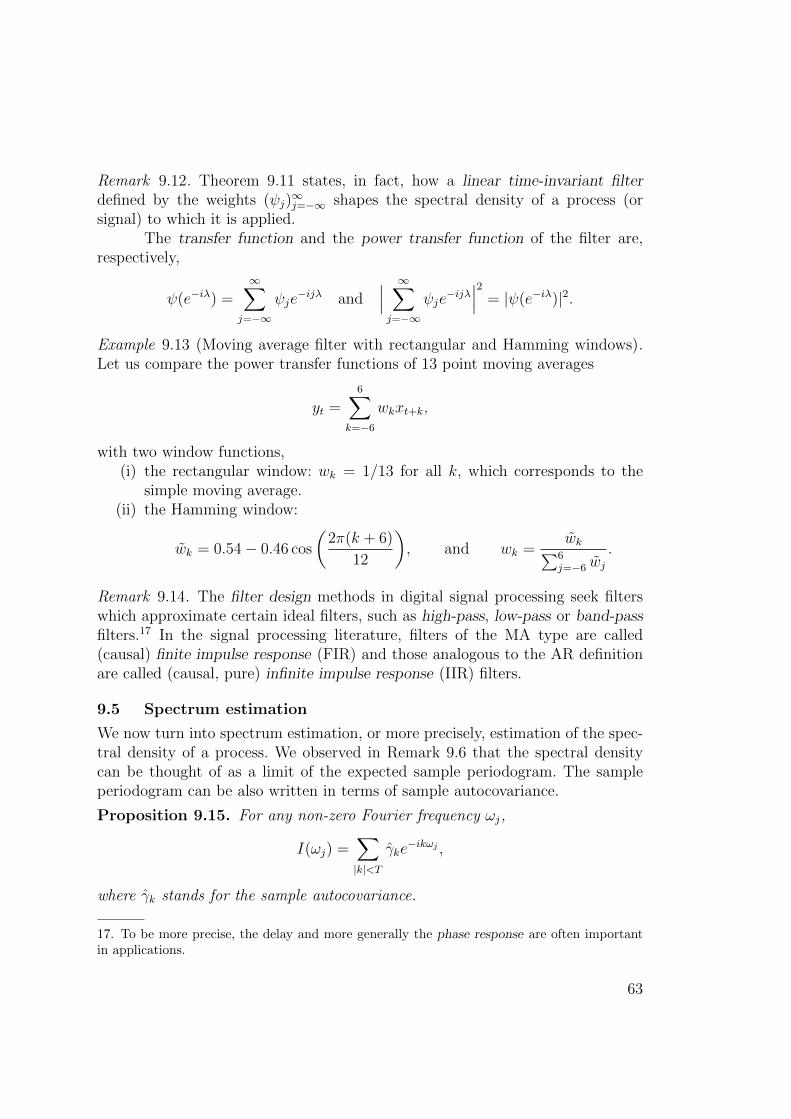
Remark 9.12. Theorem 9.11 states, in fact, how a linear time-invariant filterdefined by the weights (ψj)

∞j=−∞ shapes the spectral density of a process (or

signal) to which it is applied.The transfer function and the power transfer function of the filter are,

respectively,

ψ(e−iλ) =∞∑

j=−∞

ψje−ijλ and

∣∣∣ ∞∑j=−∞

ψje−ijλ∣∣∣2 = |ψ(e−iλ)|2.

Example 9.13 (Moving average filter with rectangular and Hamming windows).Let us compare the power transfer functions of 13 point moving averages

yt =6∑

k=−6

wkxt+k,

with two window functions,(i) the rectangular window: wk = 1/13 for all k, which corresponds to the

simple moving average.(ii) the Hamming window:

wk = 0.54− 0.46 cos

(2π(k + 6)

12

), and wk =

wk∑6j=−6 wj

.

Remark 9.14. The filter design methods in digital signal processing seek filterswhich approximate certain ideal filters, such as high-pass, low-pass or band-passfilters.17 In the signal processing literature, filters of the MA type are called(causal) finite impulse response (FIR) and those analogous to the AR definitionare called (causal, pure) infinite impulse response (IIR) filters.

9.5 Spectrum estimation

We now turn into spectrum estimation, or more precisely, estimation of the spec-tral density of a process. We observed in Remark 9.6 that the spectral densitycan be thought of as a limit of the expected sample periodogram. The sampleperiodogram can be also written in terms of sample autocovariance.

Proposition 9.15. For any non-zero Fourier frequency ωj,

I(ωj) =∑|k|<T

γke−ikωj ,

where γk stands for the sample autocovariance.

17. To be more precise, the delay and more generally the phase response are often importantin applications.

63

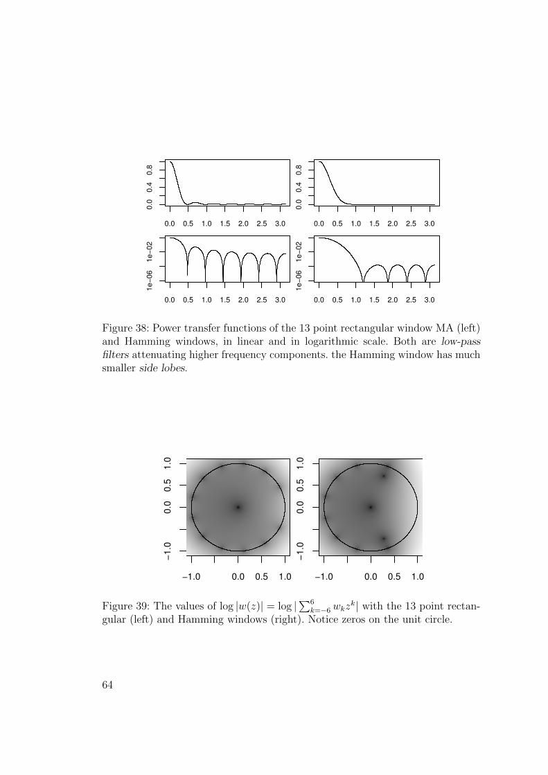
0.0 0.5 1.0 1.5 2.0 2.5 3.0

0.0

0.4

0.8

0.0 0.5 1.0 1.5 2.0 2.5 3.0

0.0

0.4

0.8

0.0 0.5 1.0 1.5 2.0 2.5 3.0

1e−

06

1e−

02

0.0 0.5 1.0 1.5 2.0 2.5 3.01e−

06

1e−

02

Figure 38: Power transfer functions of the 13 point rectangular window MA (left)and Hamming windows, in linear and in logarithmic scale. Both are low-passfilters attenuating higher frequency components. the Hamming window has muchsmaller side lobes.

−1.0 0.0 0.5 1.0

−1.0

0.0

0.5

1.0

−1.0 0.0 0.5 1.0

−1.0

0.0

0.5

1.0

Figure 39: The values of log |w(z)| = log |∑6

k=−6wkzk| with the 13 point rectan-

gular (left) and Hamming windows (right). Notice zeros on the unit circle.

64

Proof. Note that∑T

k=1 e−ikωj = 0 =

∑Tk=1 e

ikωj , and therefore

I(ωj) =1

T

( T∑k=1

(xk − µ)e−ikωj

)( T∑m=1

(xm − µ)eimωj

)∑|h|<T

e−ihωj

( 1

T

∑k,j : k−j=h

(xk − µ)(xj − µ)),

where µ := 1T

∑Tk=1 xk.

We know that the sample autocorrelation of a stationary process convergesunder general conditions (esp. for any regular ARMA). . .

Example 9.16. Consider an AR(2) with φ1 = 0.9 and φ2 = −0.7. Figure 40 showssample periodograms calculated from simulated values for a number of lengths Talong with the true spectral density.

x <- arima.sim(model=list(ar=c(0.9, -0.7)), n=2^12)

s0 <- periodogram(x[1:2^6])

s1 <- periodogram(x[1:2^8])

s2 <- periodogram(x[1:2^10])

s3 <- periodogram(x)

Proposition 9.17. Suppose (X1, . . . , XT ) is Gaussian white noise, that is,

(Xi)i.i.d.∼ N(0, σ2). Then, the periodogram I(ωj) for j = 1, . . . , [(T − 1)/2] are

i.i.d. Exp(σ−2).

Proof. Recall Remark 3.5, which say that the DFT can be written equivalentlywith a ∈ RT of a vector x ∈ RT by Ma = x, where M ∈ RT×T is an ortogonalmatrix. It follows that the vector (A1, . . . , AT ) = M−1(X1, . . . , XT ) consists of

(Ai)i.i.d.∼ N(0, σ2). Consequently, 1

σ2

(I(ωj) + I(−ωj)

) i.i.d.∼ χ2(2) = Exp(1/2). (SeeBrockwell & Davis §10.2 for details.)

Corollary 9.18. Suppose (X1, . . . , XT ) is Gaussian white noise, that is, (Xi)i.i.d.∼

N(0, σ2). Define the random variables

Yk :=

∑kj=1 I(ωj)∑[(T−1)/2]

j=1 I(ωj), k = 1, . . . ,

[T − 1

2

]− 1.

Then, Y1, . . . , Y[T−12

]−1 are distributed as the order statistics of U(0, 1) (uniform

distribution on [0, 1]), and consequently the corresponding empirical cdf has thesame distribution as empirical cdf based on [T−1

2]− 1 i.i.d. U(0, 1).

65

0.0 0.5 1.0 1.5 2.0 2.5 3.0

0.00

10.

050

1.00

0

per$freq

0.0 0.5 1.0 1.5 2.0 2.5 3.0

0.00

10.

050

1.00

0

per$freq

(per

$I)/

(2 *

pi)

0.0 0.5 1.0 1.5 2.0 2.5 3.0

0.00

10.

050

1.00

0

0.0 0.5 1.0 1.5 2.0 2.5 3.0

0.00

10.

050

1.00

0

(per

$I)/

(2 *

pi)

Figure 40: Periodograms with T = 64, 256, 1024, 4096 for AR(2) compared withthe true spectral density (in red).

The proof follows from Proposition 9.17; see Brockwell & Davis Proposi-tion 10.2.1 and Corollary 10.2.1 for details.

Example 9.19. Cumulative periodogram of the simulated AR(2) data in Example9.16, with different sample lengths.

cpgram(x[1:32], taper=0, main="T=32")

cpgram(x[1:64], taper=0, main="T=64")

cpgram(x[1:128], taper=0, main="T=128")

Example 9.16 and Proposition 9.17 suggest that the periodogram is highlyirregular, but does seem to exhibit some ‘distributional regularity.’ This is indeedtrue, for a large class of models.

In what follows, we consider the periodogram extended to all frequenciesω ∈ (0, π] by the following step-wise definition:

I(ω) := I(ωj) where j = arg minj∈FT

|ωj − ω|, (11)

and where smaller j is taken in case of ties.

66

0.0 0.1 0.2 0.3 0.4 0.5

0.0

0.2

0.4

0.6

0.8

1.0

frequency

T=32

0.0 0.1 0.2 0.3 0.4 0.50.

00.

20.

40.

60.

81.

0

frequency

T=64

0.0 0.1 0.2 0.3 0.4 0.5

0.0

0.2

0.4

0.6

0.8

1.0

frequency

T=128

0.0 0.1 0.2 0.3 0.4 0.5

0.0

0.2

0.4

0.6

0.8

1.0 T=32

0.0 0.1 0.2 0.3 0.4 0.5

0.0

0.2

0.4

0.6

0.8

1.0 T=64

0.0 0.1 0.2 0.3 0.4 0.50.

00.

20.

40.

60.

81.

0 T=128

Figure 41: Cumulative periodograms of Gaussian white noise (top) and the sim-ulated AR(2) data in Example 9.16 (bottom), with 95% confidence intervals.

Theorem 9.20. Let (Xt) be a linear process,

Xt =∞∑

j=−∞

ψjZt−j, (Zt) ∼ WN(σ2), (12)

with constants∑∞

j=−∞ |ψj| <∞. Let f stand for the spectral density of (Xt) anddenote the periodogram of X1, . . . , XT by IT .

If f > 0 on (0, π] and if 0 < λ1 < · · · < λn < π, then

1

2π

(IT (λ1), . . . , IT (λn)

) T→∞−−−→(f(λ1)E1, . . . , f(λn)En

), in distribution,

where (Ei) are independent Exp(1) random variables.

For a proof, see Brockwell & Davis Theorem 10.3.2.

Remark 9.21. Note that the expectation of the ith element on the right is f(λi),which is compatible with Remark 9.6. Recall also that any regular ARMA processis a linear process with

∑|ψj| <∞.

Theorem 9.20 suggests the intuition that the elements of the periodogramare almost independent. And if f is smooth enough, we may consider averag-ing a number of neighbouring elements to obtain a more stable spectral densityestimate.

67

Definition 9.22 (Discrete spectral average estimator). Define the weighted mov-ing average of the periodogram

f(ωj) =1

2π

m∑h=−m

w(h)I(ωj+h),

where the spectral window satisfies w(h) ≥ 0, w(h) = w(−h) and∑|h|≤mw(h) =

1, and m ≥ 1 is called its bandwidth18. The step-wise extension of f(ω) to allω ∈ (0, π] as in (11) is a discrete spectral average estimator.

The following theorem gives some guidelines about the choice of bandwidthand the window, so that the discrete spectral average estimator is consistent.

Theorem 9.23. Let fT (ω) stand for the discrete spectral average estimator basedon X1, . . . , XT and with spectral window wT (h) of bandwidth mT . Assume that asT →∞,

(i) mT →∞,(ii) mT/T → 0 and

(iii)∑|h|≤mT

w2T (h)→ 0.

Assume also that (Xt) is a linear process as in (12), with white noise havingfinite fourth moment E[Z4

j ] < ∞ and with constants∑∞

j=−∞ |ψj||j|1/2 < ∞.

Then, fT (ω) is a mean square consistent estimator of f(ω).

For a proof, see Brockwell & Davis Theorem 10.4.1 and the followingRemark 1.

In practice, we usually must choose the window for fixed T . There is acommon bias/variance tradeoff in choosing the window bandwidth.• The wider window has more averaging and hence less variance.• The wider window, the more bias (unless f is constant).

Of course, we have to choose also the window function type. Usually in practiceit is advisable to try different choices.

Remark 9.24. In this context, the rectangular window with w(h) = 12m+1

, whichcorresponds to simple moving average, is often referred to as the Daniell window.

Remark 9.25. In R, spectral average estimators can be calculated with functionspectrum, which calls spec.pgram by default. The function spec.pgram imple-ments only the Daniell window by default, with parameter spans which corre-sponds to 2m + 1. Other windows can be supplied with kernel argument. Infact spectrum supports applying multiple windowing operations by default, by

18. Sometimes the term ‘bandwidth’ is used for the bandwidth corrected with a constant whichdepends on the window type, to obtain the same asymptotic variance; see Brockwell & Davis§10.4. See also R bandwidth.kernel.

68

0.0 0.1 0.2 0.3 0.4 0.5

0.05

0.50

5.00

frequency

bandwidth = 0.00113

0.0 0.1 0.2 0.3 0.4 0.5

0.05

0.50

5.00

frequencysp

ectr

um

bandwidth = 0.00923

0.0 0.1 0.2 0.3 0.4 0.5

0.05

0.50

5.00

0.0 0.1 0.2 0.3 0.4 0.5

0.05

0.50

5.00

spec

trum

Figure 42: The spectral estimates of Example 9.26, with the true spectrum (red).The blue cross on the top right indicates variance/bandwidth (as reported by Rbandwidth.kernel).

supplying a vector in spans.19

Example 9.26. Discrete spectral averaged estimates of 256 length sample of AR(2)of Example 9.16.

spectrum(x, detrend=F)

spectrum(x, spans=9, detrend=F)

spectrum(x, spans=c(13,17), detrend=F)

spectrum(x, spans=c(25,29), detrend=F)

Figure 42 shows the spectral estimates along with the true spectrum (shown inred). Note that R spectrum does not incorporate the normalising constant 1

2πin

the estimate, for which reason the true spectral density is multiplied with 2π inFigure 42.

9.6 Parametric spectrum estimation

The discrete spectral average is a non-parametric estimate for the spectral density.It is sensible to look also for some parametric forms of spectral densities, and use

19. Recall, however, that applying multiple weighted averages consecutively is equivalent toapplying a single weighted average with window which is the convolution of the two.

69

0.0 0.1 0.2 0.3 0.4 0.5

0.05

0.50

5.00

frequencybandwidth = 0.00113

0.0 0.1 0.2 0.3 0.4 0.5

0.05

0.50

5.00

frequencysp

ectr

um

bandwidth = 0.0227

0.0 0.1 0.2 0.3 0.4 0.5

0.05

0.50

5.00

frequency

spec

trum

0.0 0.1 0.2 0.3 0.4 0.5

1e−

071e

−03

1e+

01

0.0 0.1 0.2 0.3 0.4 0.5

1e−

071e

−03

1e+

01

spec

trum

0.0 0.1 0.2 0.3 0.4 0.5

1e−

071e

−03

1e+

01

spec

trum

Figure 43: Raw periodogram, with spans=c(13,17) and the AR with AIC modelorder estimates of the AR(2) data of Example 9.16 (top) and the speech signalin Figure 14 (bottom).

them to provide spectral density estimates.The usual stationary ARMA models serve as a good candidate for the

task. There are still several choices to make, including the model order, andwhether to restrict to some sub-family such as AR or MA. Recall that AR withthe Levinson-Durbin estimation provides a sequence of models of increasing orderwith very reasonable computational requirements. Therefore, the AR models aremost commonly applied in parametric spectrum estimation. The AR spectrumestimation is often accompanied with automatic model order selection, such aswith AIC. This is what R spectrum with method="ar" does by default; see thehelp of spec.ar for details.

It is generally advisable to look both the averaged periodogram and theAR estimate, and also try different averaging (spans) and possibly different arorder (order).

70

10 State-space models

The ARIMA models all rely on the underlying assumption of stationarity. In ad-dition, the ARIMA models are defined direclty for the data. This poses problemswith various applications.

• The variance may change over time (heteroschedasticity).

• The data may be sampled irregularly.

• There may be missing data.20

This calls for more general time series models.State-space models bring a latent or unobserved layer into the model,

which allows to overcome many of the limitations of the ARIMA models. They canaccomodate time-inhomogeneity, which allows missing data or irregularly sampleddata (through continuous-time models). State-space models are still relativelysimple, but surprisingly flexible.

10.1 Linear-Gaussian state-space model

Let us start with the important special case of linear Gaussian state space mod-els. Unlike with ARIMA framework, the extension into multivariate models, isrelatively straightforward, and we will give the definition directly in this domain.

Definition 10.1 (Linear-Gaussian state-space model). Assume X0 ∼ N(µ0,Σ0)with some mean µ0 ∈ Rd and covariance matrix Σ0 ∈ Rd×d, and that for k ≥ 1

Xk = FkXk−1 +Wk (system equation)

Yk = HkXk + Uk (observation equation),

where Wk ∼ N(0,Qk) and Uk ∼ N(0,Rk), independent of each other and X0,with some covariance matrices Qk ∈ Rd×d and Rk ∈ Ro×o, and with some matricesFk ∈ Rd×d and Hk ∈ Ro×d.

Remark 10.2. Sometimes, Definition 10.1 includes additional constants in thesystem equation. However, inclusion of such constants in what follows is straight-forward; see Remark 10.15.

Remark 10.3. In the state-space model,

(i) The latent state variables (Xk)k≥1 form a Markov chain.More precisely, Xk | Xk−1 ∼ N(FkXk−1,Qk).

(ii) The observed variables (Yk)k≥1 are independent conditional on Xk.They follow Yk | Xk ∼ N(HkXk,Rk).

20. Here, we consider only missing completely at random.

71

X0 X1 X2 · · · XT

Y1 Y2 YT

(F1,W1) (F2,W2) (F3,W3) (FT ,WT )

(H1, U1) (H2, U2) (HT , UT )

Figure 44: Diagram of the linear-Gaussian state-space model (Definition 10.1).

0 50 100 150 200

−5

05

10

Figure 45: The hidden AR(1) (black) with the noisy observations (red) of Example10.4.

Example 10.4 (Noisy observations of stationary AR(1)). Let |ρ| < 1 and σ2 > 0.Define Fk = ρ and Qk = σ2, and the initial distribution

µ0 := 0 and Σ0 :=σ2

1− ρ2.

Then, (Xk)k≥0 corresponds to a stationary AR(1).Let then Hk = 1 and Rk = r2 > 0 so that Yk | Xk ∼ N(Xk, r

2) are noisyobservations of Xk (with independent noise).

This is a simulation of 200 samples from the above model with ρ = 0.9,σ2 = 1 and r = 3.

n <- 200

X <- arima.sim(model=list(ar=0.9), n=n, sd=1)

Y <- X + rnorm(n, sd=3)

Remember that the variable X would not be observed in an application, only Y.

Example 10.5 (Irregularly sampled noisy observations of Brownian motion). Let0 = t0 < t1 < · · · < tT < ∞ be some constant time points, and let σ2 > 0. Letµ0 = 0 and Σ0 > 0, and

Define Fk = 1 and let the system noise parameters satisfy

Qk := (tk − tk−1)σ2.

72

0.0 0.2 0.4 0.6 0.8 1.0

5.5

6.0

6.5

**

**

* *

*** * *

*** *

***

*

* *

*

*

* *

*

*

**

**

** *

* *

**

*

* *

Figure 46: The noisy observations (Yk) (red) of the irregularly sampled Brow-nian motion (Xk) (black). The underlying Brownian motion is also shown forillustration (gray).

Then, (Xk)k≥0 corresponds to a standard Brownian motion (Bt)t∈R+ , so thatXk = σBtk . Let then Hk = 1 and Rk = r2 > 0 as before.

This is a simulation of 20 samples from the above model with µ0 = 0,Σ0 = 32, σ2 = 1 and r = 0.2 (and with randomly picked (tk)).

n <- 20

t <- c(0,sort(runif(n))) # Random ’observation times’

W <- rnorm(n, sd=1)*sqrt(diff(t)) # The increments W_k

X0 <- rnorm(1, sd=3) # Initial state

X <- cumsum(c(X0, W)) # Construct X_k

Y <- X[-1] + rnorm(n, sd=0.2) # Simulate Y_k | X_k

Example 10.6 (ARMA(2,1)). Let the state vector be Xk = (X∗k , X∗k−1,Wk), then

Xk+1 =

X∗k+1

X∗kWk+1

=

φ1 φ2 θ11 0 00 0 0

X∗kX∗k−1Wk

+

101

Wk+1, (13)

and the observations Yk = X∗k =[1 0 0

]Xk. NB: Here Qk are singular (covari-

ance of the last term in (13)) and Rk = 0.

Example 10.7 (Random trend). Let the state vector be Xk = (Zk, Tk), and

Xk =

[1 10 1

]Xk−1 +Wk, Wk ∼ N

(0, σ2

[1/3 1/21/2 1

])Yk =

[1 0

]Xk + Uk, Uk ∼ N(0, r2).

Then, the trend Tk follows a random walk, while Zk is an “integrated” version ofTk.

73

Time

0 20 40 60 80 100

−3

02

0 20 40 60 80 100

−20

2060

***********

********

*********

**********

********

*******

*********

********

*********

****

************

*****

Figure 47: Simulated data from the random trend model in Example 10.7, withσ = 1/2 and r = 5. Top graph shows (Tk). The bottom graph shows (Zk) (black)and the observations (Yk) (red).

Remark 10.8. Example 10.7 corresponds, in fact, to a continuous-time modelwhich can be applied with irregularly sampled data. Let τk = tk − tk−1, and then

Fk =

[1 τk0 1

]and Qk = σ2

[τ 3k/3 τ 2k/2τ 2k/2 τk

].

Example 10.9 (Seasonal model). If Zk is a zero-mean seasonal hidden state, andwe would have perfect seasonality, then

∑3j=0 Sk−j = 0. We can account for

(slowly) changing seasonal effect by letting Sk = −Sk−1 − Sk−2 − Sk−3 +Wk. Wecan write this model in state space form by Xk = (Sk, Sk−1, Sk−2), that is,

Xk =

−1 −1 −11 0 00 1 0

Xk−1 +

100

Wk, Wk ∼ N(0, σ2)

Yk =[1 0 0

]Xk + Uk, Uk ∼ N(0, r2).

Remark 10.10. In state-space modelling, it is easy to combine different models.For example, it is common to have a model with both a random trend model suchas in Example 10.7 and a seasonal model such as in Example 10.9, and model theobservation as being Yk = Zk + Sk + Uk, where Uk ∼ N(0, r2).

74

0 10 20 30 40

−5

05

**

**

*

*

*

**

*

**

*

*

**

**

**

* *

**

**

*

*

*

**

*

*

**

*

*

*

*

*

Figure 48: Simulated data from the seasonal model with σ = r = 1.

Remark 10.11 (*). Durbin & Koopman promote the use of diffuse initialisationof the Kalman filter (or the state-space model). This means considering the limitof mk|k and Pk|k as µ0 = 0 and Σ0 = αI, and we let α → ∞ (when the limitexists).

10.2 State inference in linear-Gaussian state-space model

Our first aim is to calculate the conditional distribution of the latentvariables X1, . . . , XT given observations Y1 = y1, . . . , YT = yT . Because(X1, . . . , XT , Y1, . . . , YT ) is Gaussian (with dimension (d + o)T ), we could inprinciple derive the conditional mean and covariance of X1, . . . , XT givenY1 = y1, . . . , YT = yT by matrix algebra.

However, if T is large, the matrices are large, and the approach wouldquickly get computationally expensive (or intractable). Fortunately, the specificstructure of the model allows much more efficient approach for calculating theconditional means and covariances sequentially.

Definition 10.12 (Conditional means and variances). For 0 ≤ a ≤ b ≤ T ,we shall use the notation Xa:b = (Xa, . . . , Xb), and we assume that y1:T is theobserved data. For k, j = 0, . . . , T we denote

mj|k := E[Xj | Y1:k = y1:k]

Pj|k := Var(Xj | Y1:k = y1:k),

where Var( · ) means the (conditional) covariance matrix of the argument. Wefurther define (mj|0,Pj|0) as the unconditional mean and covariance, so thatm0|0 = µ0 and P0|0 = Σ0.

We start by looking how we may calculate (m1|1,P1|1),(m2|2,P2|2), . . . , (mT |T ,PT |T ), so that then

Xk | (Y1:k = y1:k) ∼ N(mk|k,Pk|k).

This is called filtering in the state-space context.

75

Lemma 10.13. Suppose X1 and X2 be random vectors which are jointly Gaus-sian. Let µi = E[Xi] and Σij = Cov(Xi, Xj). If Σ22 is invertible, then,

E[X1 | X2 = x2] = µ1 + Σ12Σ−122 (x2 − µ2)

Var(X1 | X2 = x2) = Σ11 − Σ12Σ−122 Σ21.

Proof. Define A := −Σ12Σ−122 and Z = X1 + AX2, then

Cov(Z,X2) = Cov(X1, X2) + A Cov(X2, X2) = 0,

so Z is indepedent of X2. Now,

E[X1 | X2 = x2] = E[Z − AX2 | X2 = x2]

= E[Z]− Ax2 = µ1 + A(µ2 − x2).

We also have Var(X1 | X2 = x2) = Var(Z − AX2 | X2 = x2) = Var(Z), and

Var(Z) = Var(X1 + AX2)

= Σ11 + AΣ21 + Σ12AT + AΣ22A

T = Σ11 − Σ12Σ−122 Σ21.

Algorithm 10.14 (The Kalman filter). For k = 1, 2, . . . , T , calculate the pre-dicted mean and covariance

mk|k−1 = Fkmk−1|k−1 (14)

Pk|k−1 = FkPk−1|k−1FTk + Qk, (15)

and then the update

zk = yk − Hkmk|k−1 (16)

Sk = HkPk|k−1HTk + Rk (17)

mk|k = mk|k−1 + Pk|k−1HTk S−1k zk (18)

Pk|k = (I − Pk|k−1HTk S−1k Hk)Pk|k−1. (19)

Proof of Algorithm 10.14. The prediction is relatively straightforward:

mk|k−1 = E[FkXk−1 +Wk | Y1:k−1 = y1:k−1] = Fkmk−1|k−1

Pk|k−1 = Var(FkXk−1 +Wk | Y1:k−1 = y1:k−1) = FkPk−1|k−1FTk + Qk.

For update, let us observe that the joint distribution of (Xk, Yk) given Y1:k−1 =y1:k−1 is a Gaussian with mean and covariance

µ :=

[mk|k−1

Hkmk|k−1

], Σ :=

[Pk|k−1 Pk|k−1H

Tk

HkPk|k−1 Sk

].

76

Now, we aim to look at conditional of this distribution, when setting Yk = yk.We may apply Lemma 10.13 with µ1 = mk|k−1, µ2 = Hkmk|k−1, Σ11 = Pk|k−1,Σ12 = Pk|k−1H

Tk , Σ21 = HkPk|k−1 and Σ22 = Sk, then

mk|k = mk|k−1 + Pk|k−1HTk S−1k (yk − Hkmk|k−1)

Pk|k = Pk|k−1 − Pk|k−1HTk S−1k HkPk|k−1.

Remark 10.15. In the Algorithm 10.14,

(i) If the system equation involves additional constants, such that Xk =FkXk−1 +Wk + bk, then, the algorithm applies with (14) changed to

mk|k−1 = Fkmk−1|k−1 + bk. (14’)

(ii) In case of missing observations (completely at random), the Kalman filterupdate consists only of prediction equations, and the update equations(16)–(19) are skipped. That is, mk|k = mk|k−1 and Pk|k = Pk|k−1.

(iii) The residual terms zk are often called innovations and similarly Sk are theinnovation covariances.

(iv) Direct implementation of the update equations (18) and (19) with matrixinverses may be numerically unstable. In fact, valid updates exist also fornon-invertible Sk.

Proposition 10.16. Consider a family of state-space models Γ(θ) =(µ

(θ)0 ,Σ

(θ)0 , (F

(θ)k ), (H

(θ)k ), (Q

(θ)k ), (Rk)

(θ)), indexed by parameter θ. The likelihoodof θ given an observation sequence y1:T can be obtained from Algorithm 10.14applied with the parameters Γ(θ), from

L(θ; y1:T ) =T∏k=1

N(zk; 0, Sk).

Proof. Write

L(θ; y1:T ) = p(y1)T∏k=2

p(yk | y1:k−1),

and recall from the proof of Algorithm 10.14 that the conditional distributionsYk|Y1:k−1 = y1:k−1 are N(Hkmk|k, Sk), so the conditional distribution of Zk =Yk −Hkmk|k is N(0, Sk).

Hidden state and observation prediction come directly from the Kalmanfilter.

Algorithm 10.17 (Prediction with Kalman filter). For k = T + 1, . . . , T + k,

77

(i) calculate state predictions

mk|T = Fkmk−1|T

Pk|T = FkPk−1|TFTk + Qk,

(ii) calculate observation predictions yk|T = E[Yk | Y1:T = y1:T ] and their

covariances Sk|T with

yk|T = Hkmk|T

Sk|T = HkPk|THTk + Rk.

We next look how the conditional means and covariances mk|T and Pk|Tare determined. This is called smoothing in the state-space context.

Algorithm 10.18 (The Kalman smoother). For k = T−1, T−2, . . . , 1, calculatethe smoothed mean and covariance as follows

mk|T = mk|k + Ck(mk+1|T −mk+1|k) (20)

Pk|T = Pk|k + Ck(Pk+1|T − Pk+1|k)CTk , (21)

where Ck = Pk|kFTk+1P

−1k+1|k.

Remark 10.19. In Algorithm 10.18,(i) Missing observations are handled automatically (note also that (20) and

(21) do not depend on data).(ii) Direct implementation of the Kalman smoother may be numerically un-

stable. There exist techniques which are more general and stable.

Proof of Algorithm 10.18. Similar as in Proof of Algorithm 10.14, we see that(Xk, Xk+1) | Y1:k = y1:k has mean and covariance

µ :=

[mk|k

mk+1|k

], Σ :=

[Pk|k Pk|kF

Tk+1

Fk+1Pk|k Pk+1|k

],

and then the distribution of Xk | Xk+1, Y1:k = y1:k has mean and covariance

Mk := mk|k + Pk|kFTk+1P

−1k+1|k(Xk+1 −mk+1|k)

= mk|k + Ck(Xk+1 −mk+1|k)

Sk := Pk|k − Pk|kFTk+1P

−1k+1|kFk+1Pk|k

= Pk|k − CkPk+1|kCTk

Now, because Xk is conditionally independent of Yk+1:T given Xk+1, we get (20)from

E[Xk | Y1:T = y1:T ] = E[E[Xk | Xk+1, Y1:T = y1:T ] | Y1:T = y1:T ]

78

0 50 100 150 200

−5

05

10

**

***

*

*

***

*

*****

*

**

*

***

*

*

*

**

*

*

*

***

*

*

*****

*

*

*

*

*

****

*

******

**

*

*

*

****

*

*

*

*

*

*

*

**

*

*

*

******

**

***

*

*

**

*

*

**

*

*

*

********

*

*

*

*

*

**

*

*

***

*

**

*

*

*

***

**

***

*

**

****

**

*

**

*****

**

*

****

*

*

*

**

*

*

*

***

***

*

**

*

**

*

**

***

*

*

**

****

*

***

**

**

Figure 49: The smoothed mean mk|T (blue) and the 50% and 95% confidenceintervals corresponding Pk|T (gray).

= E[Mk | Y1:T = y1:T ].

By the law of total (conditional) (co)variance,

Var(Xk | Y1:T = y1:T ) = E[Var(Xk | Xk+1, Y1:T = y1:T ) | Y1:T = y1:T ]

+ Var(E[Xk | Xk+1, Y1:T = y1:T ] | Y1:T = y1:T ).

The first term on the right equals Sk and the latter equals

Var(Mk | Y1:T = y1:T ) = Var(CkXk+1 | Y1:T = y1:T ) = CkPk+1|TCTk .

Example 10.20. Kalman smoother applied to the noisy AR(1) observations (Yk)in Example 10.4

# Do install.packages("KFAS") first to install the package!

require(KFAS)

# Define the model parameters for KFAS

rho <- 0.9; sigma <- 1; r <- 3

model <- SSModel(Y ~ -1 + SSMarima(ar=rho, Q=sigma^2), H=r^2)

# Run Kalman filter & smoother:

out <- KFS(model)

# Extract mean and variance of the smoothed state:

m <- out$alphahat

P <- out$V[1,1,]

Example 10.21. Kalman smoother applied to the noisy observations of a Brown-ian motion in Example 10.5.

79

0.0 0.2 0.4 0.6 0.8 1.0

5.0

5.5

6.0

6.5

**

**

*

*

** *

* ***

* **** *

Figure 50: The smoothed mean mk|T (blue) and the 50% and 95% confidenceintervals corresponding Pk|T (gray).

require(KFAS)

# Include intermediate time instants spaced with dt

t_ <- sort(union(t, seq(0,1,by=1/512)))

n_ <- length(t_); Y_ <- rep(NA, n_)

for (k in 2:n) {

j <- which(t_ == t[k]); Y_[j] <- Y[k]

}

# Now Q changes in time; it can be encoded as follows

Q <- array(c(diff(t_)), c(1, 1, length(Y_)))

# Define the model

mod <- SSModel(Y_ ~ SSMtrend(1, Q = list(Q), P1 = 3^2), H = 0.2^2)

out <- KFS(mod)

m <- out$alphahat

P <- out$V[1,1,]

10.3 Maximum likelihood inference in linear-Gaussian state-spacemodels

In order to fit a state-space model, the observation of Proposition 10.16 is veryuseful. In case we look for maximum likelihood estimates θ, we must search for θthat maximises the (log-)likelihood from the Kalman filter. While specific state-space models may admit more efficient estimation methods, we may also max-imise the likelihood taken as a ‘black box’. We may also construct (approximate,asymptotic) confidence intervals from the inverse Hessian.

Example 10.22. Finding the MLE of θ = (ρ, σ, r) in the noisy AR(1) parameters

80

332

334

336

338

338

340

340

342

342

344

344

346

0.0 0.5 1.0 1.5

0.0

0.2

0.4

0.6

0.8

1.0

335

340

345

345 345

350

350

355

355

360 365

0.5 1.0 1.52.

02.

53.

03.

54.

0

(a) (b)

Figure 51: Negative log-likelihood surface of data from noisy AR(1) Example 10.4:(a) over a range of values of σ (x axis) and ρ (y axis), with r = 32. (b) over arange of values of σ (x axis) and r (y axis), with ρ = 0.9.

(Example 10.4).

require(KFAS)

# Function which returns a model built with given parameters

build <- function(parm, model) {

SSModel(model$y ~ -1 +

SSMarima(ar=parm[1], Q=parm[2]^2), H=parm[3]^2)

}

# Use fitSSM routine (a wrapper for R optim)

fit <- fitSSM(model=list(y=Y), c(0,1,1), build, hessian=T,

method="L-BFGS-B",

lower=c(-.99,0.01,0.01), upper=c(.99,NA,NA))

mle <- fit$optim.out$par

c95.d <- sqrt(diag(solve(fit$optim.out$hessian)))*1.96

The found estimates were approximately ρ = 0.93 ± 0.09, σ = 0.62 ± 0.45 andr = 2.93± 0.34.

Given a MLE θ, we may use the model with parameters θ in order to:

(i) Calculate estimated trajectory of the latent variables X1:T (smoothing).

(ii) Calculate predictions for the latent variables XT+1:T+p.

(iii) Calculate predictions for the future observations YT+1:T+p.

Example 10.23. Continuing from Example 10.22, we may use KFAS in order to

81

160 180 200 220 240

−6

−2

24

6

**

****

**

*

**

*

*

***

*

*

*

*

***

*

*

*

**

*

*

*

*

**

***

*

**

*

*

*

*

*

*

***

*

*

*

*

*

***

*

***

*

*

*

*

Figure 52: Smoothed state estimates, state and observation predictions of thenoisy AR(1) from Example 10.23.

perform the above tasks.

n.ahead <- 50

m <- predict(fit$model, interval="confidence", level=0.95)

m.pred <- predict(fit$model, n.ahead=n.ahead,

interval="confidence", level=0.95)

y.pred <- predict(fit$model, n.ahead=n.ahead,

interval="prediction", level=0.95)

ts.plot(m, m.pred, y.pred[,2:3], col=c(1,1,1,4,4,4,3,3),

lty=c(1,2,2,1,2,2,2,2), xlim=c(150,n+n.ahead))

points(Y, type="p", pch="*", col=2)

Example 10.24. Decomposition of the AirPassengers data using nearly seasonaland random walk ‘local linear trend’ models.

y <- log(AirPassengers)

model <- SSModel(y ~ SSMtrend(1, Q=list(NA)) +

SSMseasonal(period=12, Q=NA), H=NA)

# all unknown parameters are in Q and H, no need for buildfn

fit <- fitSSM(model, inits = c(-1,-1,-1), method = "BFGS")

fm <- fit$model

pred <- predict(fm, interval="p", level=0.95, n.ahead=24)

p.s.t <- predict(fm, interval="c", level=0.95, states=1)

p.t <- predict(fm, interval="c", level=0.95, states=1, n.ahead=24)

p.s.s <- predict(fm, interval="c", level=0.95, states=2)

p.s <- predict(fm, interval="c", level=0.95, states=2, n.ahead=24)

82

Time

1950 1952 1954 1956 1958 1960 1962

5.0

6.0

Time

1950 1952 1954 1956 1958 1960 1962

5.0

6.0

1950 1952 1954 1956 1958 1960 1962

−0.

20.

00.

2

Figure 53: Decomposition of the air passengers data in Example 10.24 with 24month predictions.

10.4 On Bayesian inference for linear-Gaussian state-space models

In state-space modelling, it is easy to end up with weak identifiability (or evennon-identifiability) especially with more complicated models. Even if the maxi-mum likelihood estimates may be found, the uncertainty related to the estimatesmay well be substantial, and disregarding the parameter uncertainty in predic-tions may lead to overly optimistic confidence bounds. It is increasingly commonto use a (fully) Bayesian approach, and set a prior for the unknown parameterspr(θ). In that case, the inference is usually based on posterior expectations (orprobabilities).

A fully Bayesian state-space model is based on a joint distribution on(θ,X1:T , Y1:T ), which takes the general form

p(θ, x1:T , y1:t) = pr(θ)p(x1:T , y1:T | θ),where p(x1:T , y1:T | θ) corresponds to a linear-Gaussian SSM. The inference withobserved y1:T is based on the posterior density which can be written in the form

π(θ, x1:T ) := p(θ, x1:T | y1:T ) ∝ p(x1:T | y1:T , θ)p(θ, y1:T ) = pr(θ)L(θ)p(x1:T | y1:T , θ),where L(θ) is the likelihood from the Kalman filter applied with parameters θ (seeProposition 10.16), and p(x1:T | y1:T , θ) is a Gaussian distribution, with marginalscalculated by the Kalman smoother.

83

Algorithm 10.25 (MCMC for linear-Gaussian SSM). Pick some initial valuesθ0 and a proposal density q( · | θ), then for k = 1, . . . , n:

(i) Draw θ′k ∼ q( · | θk−1)(ii) With probability

min

{1,

pr(θ′k)L(θ′k)q(θk−1 | θ′k)pr(θk−1)L(θk−1)q(θ′k | θk−1)

},

accept and set θk = θ′k; otherwise reject and set θk = θk−1.

Remark 10.26. The output (θb, . . . , θn) of Algorithm 10.25 can be regarded asan empirical approximation of the marginal p(θ | Y1:T = y1:T ) ≈ (n − b +1)−1

∑nk=b δθk , and the smoothing marginal is approximated by a mixture of Gaus-

sians p(x1:T | Y1:T = y1:T ) ≈ (n− b+ 1)−1∑n

k=b p(x1:T | y1:T , θk). Generally,∫h(θ, x1:T )dθdx1:T ≈

1

n

n∑k=1

∫h(θk, x1:T )p(x1:T | y1:T , θk)dx1:T .

Example 10.27. MCMC for noisy AR(1) in Example 10.4.

build <- function(p, y) {

rho <- (1-exp(p[1]))/(1+exp(p[1])) # Transformations ensure

Q <- exp(p[2]); H <- exp(p[3]) # right range of values

SSModel(y ~ -1 + SSMarima(ar=rho, Q=Q), H=H)

}

theta <- c(0,1,1); n <- 5000

Theta <- matrix(NA, ncol=n, nrow=3)

L <- logLik(build(theta, Y))

for (k in 1:n) {

theta_ <- theta + rnorm(3, sd=0.3) # Symmetric random walk q

L_ <- logLik(build(theta_, Y)) # Uniform (improper) prior

if (runif(1)<=exp(L_-L)) {

theta <- theta_; L <- L_ # Accept

}

Theta[,k] <- theta

}

Calculating the estimates of means and variances of the smoothing distributionbased on MCMC output

b <- ceiling(n/5) # "burn-in"

theta <- Theta[,b]; o <- KFS(build(theta,Y))

m <- m_ <- o$alphahat; P_ <- o$V[1,1,]; Pm <- P_+m_^2

for (k in (b+1):n) {

84

0 50 100 150 200

−10

−5

05

*

*

***

*

*

**

*

*

**

***

*

*

*

*

*

**

*

*

*

**

*

*

*

**

*

*

*

***

*

*

*

*

*

*

****

*

**

***

*

**

*

*

*

****

*

*

*

*

*

*

*

**

*

*

*

******

*

*

**

*

*

*

*

*

*

*

**

*

*

*

*

*

**

****

*

*

*

*

*

**

*

*

**

*

*

*

*

*

*

***

**

**

*

*

**

****

**

*

*

*

*

*

**

*

*

*

*

*

***

*

*

*

*

*

*

*

*

*

**

***

*

**

*

*

*

*

*

*

**

*

*

*

*

*

*

***

*

***

*

*

*

*

Figure 54: Posterior mean & 1.96×posterior sd (black) of the smoothing distri-bution (Example 10.27), compared to ML fitted model smoothing distribution(blue).

theta_ <- Theta[,k]

if (any(theta != theta_)) {

theta <- theta_; o <- KFS(build(theta,Y))

m_ <- o$alphahat; P_ <- o$V[1,1,]

}

g <- 1/(k-b+1)

m <- (1-g)*m + g*m_

Pm <- (1-g)*Pm + g*(P_+m_^2)

}

P <- Pm - m^2

10.5 Hidden Markov models

Definition 10.28 (Hidden Markov model). A hidden Markov model consistsof a Markov state (X1:T ) and where Xk take values in {1, . . . ,m}, and Y1:T areconditionally independent given X0:T . The parameters of the model are:

(a) X0 ∼ µ0 (initial distribution)

(b) Pr(Xk = j | Xk−1 = i) = Tk(i, j) (transition probability)

(c) Yk | (Xk = i) ∼ gk( · | i) (‘emission’ distribution; discrete or continuous)

Denote similarly as in the linear-Gaussian case pj|k(i) = Pr(Xj = i |Y1:k = y1:k). Then, the filtering distributions pk|k, the smoothing distributionspk|T , as well as the likelihood L, may be calculated in O(m2T ) time, using the

85

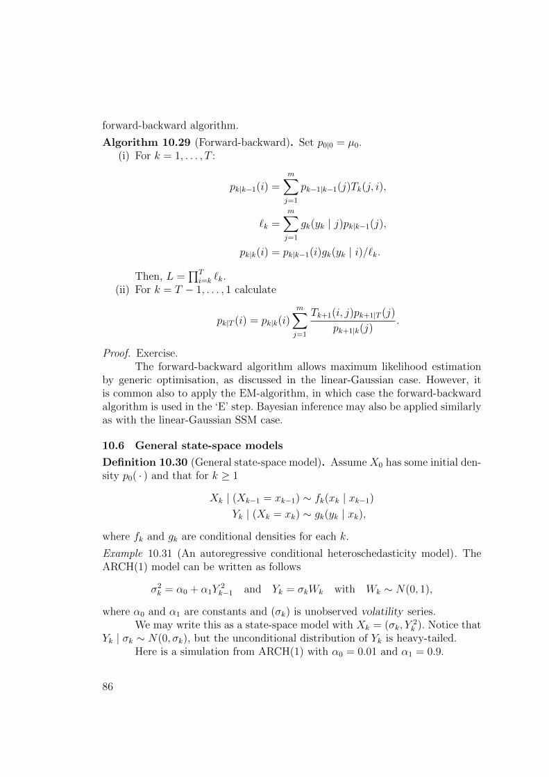
forward-backward algorithm.

Algorithm 10.29 (Forward-backward). Set p0|0 = µ0.(i) For k = 1, . . . , T :

pk|k−1(i) =m∑j=1

pk−1|k−1(j)Tk(j, i),

`k =m∑j=1

gk(yk | j)pk|k−1(j),

pk|k(i) = pk|k−1(i)gk(yk | i)/`k.

Then, L =∏T

i=k `k.(ii) For k = T − 1, . . . , 1 calculate

pk|T (i) = pk|k(i)m∑j=1

Tk+1(i, j)pk+1|T (j)

pk+1|k(j).

Proof. Exercise.The forward-backward algorithm allows maximum likelihood estimation

by generic optimisation, as discussed in the linear-Gaussian case. However, itis common also to apply the EM-algorithm, in which case the forward-backwardalgorithm is used in the ‘E’ step. Bayesian inference may also be applied similarlyas with the linear-Gaussian SSM case.

10.6 General state-space models

Definition 10.30 (General state-space model). Assume X0 has some initial den-sity p0( · ) and that for k ≥ 1

Xk | (Xk−1 = xk−1) ∼ fk(xk | xk−1)Yk | (Xk = xk) ∼ gk(yk | xk),

where fk and gk are conditional densities for each k.

Example 10.31 (An autoregressive conditional heteroschedasticity model). TheARCH(1) model can be written as follows

σ2k = α0 + α1Y

2k−1 and Yk = σkWk with Wk ∼ N(0, 1),

where α0 and α1 are constants and (σk) is unobserved volatility series.We may write this as a state-space model with Xk = (σk, Y

2k ). Notice that

Yk | σk ∼ N(0, σk), but the unconditional distribution of Yk is heavy-tailed.Here is a simulation from ARCH(1) with α0 = 0.01 and α1 = 0.9.

86

0 50 100 150 200 250 300

−1.

5−

0.5

0.5

1.5

Figure 55: The simulated values Yk from ARCH(1) of Example 10.31, with theconfidence intervals of the conditional Yk given σk−1. The data Yk shows het-eroschedasticity (volatility clustering).

n <- 300; alpha0 <- 0.01; alpha1 <- 0.9

Y <- S <- rep(NA, n); S[1]=0.5

Y[1] <- rnorm(1, sd=S[1])

for (k in 2:n) {

S[k] <- alpha0 + alpha1*Y[k-1]^2

Y[k] <- rnorm(1, sd=sqrt(S[k]))

}

Example 10.32 (A stochastic volatility model). Suppose that ρ ∈ (0, 1), q > 0and (Xk) is a stationary AR(1), that is, X0 ∼ N

(0, 1

1−ρ2)

and

Xk = ρXk−1 +Wk, Wk ∼ N(0, q).

The observations follow

Yk = σ exp(1

2Xk

)Uk, Uk ∼ N(0, 1),

where the standard deviation σ is a constant.The term σ exp

(12Xk

)plays a similar role as the σk in the ARCH(1). Here

is a simulation of the SV model with same AR(a) parameters as in Example 10.4and with σ = 2.

n <- 200

X <- arima.sim(model=list(ar=0.9), n=n, sd=1)

Y <- exp(X/2)*rnorm(n, sd=2)

87

0 50 100 150 200

−20

010

Figure 56: The simulated series (Yk) from the SV model, with confidence boundsof the conditional distributions Yk | Xk as in Figure 55.

−1.

5−

0.5

0.5

1.5

50 100 150 200 250

Figure 57: The latent random walk (Xk) (top) and the binary observations (Yk)(bottom) of Example 10.34.

Remark 10.33. There are more complicated versions of both the ARCH and theSV models. The generalised ARCH model GARCH(p,q) assumes the volatility tofollow

σ2k = α0 +

q∑j=1

αjY2k−j +

p∑j=1

βjσ2k−j.

The ARCH(q)=GARCH(0,q) is an obvious extension of ARCH(1), butGARCH(p,0) can be thought of a SV model.

Example 10.34 (Binary observations with random-walk logit probabilities). Sup-pose (Xk) is a Gaussian random walk with X0 = 0 and σ = 50, and Pr(Yk = 1 |Xk) = logit−1(Xk) = 1− Pr(Yk = 0).

88

10.7 State inference in general state-space models

Definition 10.35 (Conditional densities). For k, j = 0, . . . , T we denote bypj|k( · ) the conditional densities of Xj | Y1:k = y1:k, that is,

P(Xj ∈ A | Y1:k = y1:k) =

∫A

pj|k(xj)dxj.

In particular, pk|k are the filtering densities and pk|T the smoothing densities.

Apart from specific cases, notably the linear-Gaussian SSM and the HMM,inference in a general state-space model is based on approximations.

Remark 10.36. In case the model exhibits linear structure, with non-Gaussiannoise, that is

Xk = FkXk−1 +Wk, Yk = HkXk + Uk,

where Wk and Uk are zero-mean and have finite covariances Qk and Rk, butmay be non-Gaussian, then the Kalman filter may still be applied, and viewedas a ‘least squares’ estimation method. Note that then the (exact) likelihood isunavailable.

There are two major brances of approximations available. One branch isto stick with the ‘Kalman filter type’ approach and approximate pk|k and pk|Twith Gaussians (or with mean and covariance). Such methods often work wellif the model is regular enough so that the true posteriors are reasonably wellapproximated by Gaussians (or summarised by mean and covariance).

If that is not the case, there are efficient sequential Monte Carlo methodswhich approximate pk|k and pk|T in a non-parametric manner, by a large number ofrandom samples (often referred to as ‘particles’). In particular, the particle filterand particle smoother algorithms can often provide very accurate approximationsin many cases with reasonable computational cost.21

Let us take a closer look in a widely used approach called the extendedKalman filter, in case of Gaussian noise, but non-linear dependences.

Definition 10.37 (Gaussian state space model with non-linear dynamics). As-sume X0 ∼ N(µ0,Σ0) with some mean µ0 ∈ Rd and covariance matrix Σ0 ∈ Rd×d,and that for k ≥ 1

Xk = fk(Xk−1) +Wk Wk ∼ N(0,Qk)

Yk = hk(Xk) + Uk Uk ∼ N(0,Rk),

with some continuously differentiable functions fk : Rd → Rd and h : Rd → Ro.

21. See for instance Cappe, Moulines & Ryden, Inference in Hidden Markov Models, Springer,2005.

89

Algorithm 10.38 (The extended Kalman filter). Assume the model in Defini-tion 10.37. The EKF is identical to the Kalman filter Algorithm 10.14, except of(14) and (16) replaced with

mk|k−1 = fk(mk−1|k−1) and zk = yk − hk(mk|k−1),

respectively, and using the following matrices

Fk := f ′k(mk−1|k−1) and Hk := h′k(mk|k−1).

Remark 10.39. The extended Kalman filter can be defined also for a model in-corporating non-additive and non-Gaussian noise, by letting

Xk = fk(Xk−1,Wk), Yk = hk(Xk, Uk).

Then, the noise matrices Qk and Rk are corrected by a similar linearisation. Thereare also several other ‘extensions’ of the Kalman filter, which aim at providing amore accurate approximation.

Remark 10.40. If the state variables (Xk) follow a linear-Gaussian model, but therelationship Yk | Xk is non-linear or non-Gaussian, but belonging to the expo-nential family, then Durbin & Koopman suggest to use Laplace approximations,which are found iteratively by running the Kalman smoother with linearised ob-servation equation, and re-linearising the observation equation at new smoothedstates. This is how the KFAS package handles observations from Poisson, binomial,Gamma and negative binomial distributions.

Example 10.41. Maximum likelihood estimation in the binary observations Ex-ample 10.34:

require(KFAS)

# Instead of "H", supply name of the observation distribution.

# in case of binomial, u is the size.

mod <- SSModel(y ~ SSMtrend(1, Q=list(NA)),

distribution="binomial", u=1)

fit <- fitSSM(mod, inits=c(1), method="BFGS")

s.x <- predict(fit$model, interval="c", level=0.95)

p.x <- predict(fit$model, interval="c", level=0.95, n.ahead=50)

10.8 On Bayes inference in general state-space models

With linear-Gaussian models, the MCMC could be performed only on the pa-rameters θk, because of the access to the (marginal) likelihood from the Kalmanfilter. In the general state-space models, the straightforward approach would be

90

Time

0 50 100 150 200 250 300

−4

−2

01

2

50 100 150 200 250 300

Figure 58: Example 10.34; confidence intervals for the smoothing distribution(blue) and the predictions (red).

to do MCMC jointly on the latent variable and parameter space (x1:T , θ). How-ever, this can be prohibitively inefficient in many cases, if T is even moderatelylarge.

The recent particle MCMC methods combine efficient sequential MonteCarlo (or particle filter) algorithms, which are used ‘in place of’ the Kalman filterin Algorithm 10.25. Rather surprisingly, this can be easily implemented so thatthe method defines a valid MCMC for the joint posterior p(θ, x1:T | y1:T ). 22 Suchmethods have enabled inference in moderate-sized general state-space models,but general, easy-to-use packages which implement these methods efficiently arestill under development.

22. For further discussion, see for instance a recent review article: Kantas, Doucet, Singh,Maciejowski & Chopin: On particle methods for parameter estimation in state-space models,Statist. Sci. 30(3):328–351 (2015).

91