Computational Materials Science 47 (2009) 237–253

Contents lists available at ScienceDirect

Computational Materials Science

journal homepage: www.elsevier .com/locate /commatsci

Density-functional tight-binding for beginners

Pekka Koskinen *, Ville MäkinenNanoScience Center, Department of Physics, University of Jyväskylä, 40014 Jyväskylä, Finland

a r t i c l e i n f o

Article history:Received 1 June 2009Accepted 29 July 2009Available online 22 August 2009

PACS:31.10.+z71.15.Dx71.15.Nc31.15.E�

Keywords:DFTBTight-bindingDensity-functional theoryElectronic structure simulations

0927-0256/$ - see front matter � 2009 Elsevier B.V. Adoi:10.1016/j.commatsci.2009.07.013

* Corresponding author. Tel.: +358 14 260 4717.E-mail address: pekka.koskinen@iki.fi (P. Koskinen

a b s t r a c t

This article is a pedagogical introduction to density-functional tight-binding (DFTB) method. We derive itfrom the density-functional theory, give the details behind the tight-binding formalism, and give practi-cal recipes for parametrization: how to calculate pseudo-atomic orbitals and matrix elements, and espe-cially how to systematically fit the short-range repulsions. Our scope is neither to provide a historicalreview nor to make performance comparisons, but to give beginner’s guide for this approximate, butin many ways invaluable, electronic structure simulation method—now freely available as an open-source software package, hotbit.

� 2009 Elsevier B.V. All rights reserved.

1. Introduction

If you were given only one method for electronic structure calcu-lations, which method would you choose? It certainly depends onyour field of research, but, on average, the usual choice is probablydensity-functional theory (DFT). It is not the best method for every-thing, but its efficiency and accuracy are suitable for most purposes.You may disagree with this argument, but already DFT commu-nity’s size is a convincing evidence of DFT’s importance—it is evenamong the few quantum mechanical methods used in industry.

Things were different before. When computational resourceswere modest and DFT functionals inaccurate, classical force fields,semiempirical tight-binding, and jellium DFT calculations wereused. Today tight-binding is mostly familiar from solid-state text-books as a method for modeling band-structures, with one to sev-eral fitted hopping parameters [1]. However, tight-binding couldbe used better than this more often even today—especially as amethod to calculate total energies. Particularly useful for total en-ergy calculations is density-functional tight-binding, which isparametrized directly using DFT, and is hence rooted in first prin-ciples deeper than other tight-binding flavors. It just happened thatdensity-functional tight-binding came into existence some tenyears ago [2,3] when atomistic DFT calculations for realistic system

ll rights reserved.

).

sizes were already possible. With DFT as a competitor, the DFTBcommunity never grew large.

Despite being superseded by DFT, DFTB is still useful in manyways: (i) In calculations of large systems [4,5]. Computational scal-ing of DFT limits system sizes, while better scaling is easier to achievewith DFTB. (ii) Accessing longer time scales. Systems that are limitedfor optimization in DFT can be used for extensive studies on dynam-ical properties in DFTB [6]. (iii) Structure search and general trends[7]. Where DFT is limited to only a few systems, DFTB can be usedto gather statistics and trends from structural families. It can be usedalso for pre-screening of systems for subsequent DFT calculations[8,9]. (iv) Method development. The formalism is akin to that ofDFT, so methodology improvements, quick to test in DFTB, can beeasily exported and extended into DFT[10]. (v) Testing, playingaround, learning and teaching. DFTB can be used simply for playingaround, getting the feeling of the motion of atoms at a given temper-ature, and looking at the chemical bonding or realistic molecularwavefunctions, even with real-time simulations in a classroom—DFTB runs easily on a laptop computer.

DFTB is evidently not an ab initio method since it containsparameters, even though most of them have a theoretically solidbasis. With parameters in the right place, however, computationaleffort can be reduced enormously while maintaining a reasonableaccuracy. This is why DFTB compares well with full DFT withminimal basis, for instance. Semiempirical tight-binding can beaccurately fitted for a given test set, but transferability is usually

238 P. Koskinen, V. Mäkinen / Computational Materials Science 47 (2009) 237–253

worse; for general purposes DFTB is a good choice among the dif-ferent tight-binding flavors.

Despite having its origin in DFT, one has to bear in mind that DFTBis still a tight-binding method, and should not generally be consid-ered to have the accuracy of full DFT. Absolute transferability cannever be achieved, as the fundamental starting point is tightly boundelectrons, with interactions ultimately treated perturbatively. DFTBis hence ideally suited for covalent systems such as hydrocarbons[2,11]. Nevertheless, it does perform surprisingly well describingalso metallic bonding with delocalized valence electrons [12,8].

This article is neither a historical review of different flavors oftight-binding, nor a review of even DFTB and its successes or failures.For these purposes there are several good reviews, see, for exampleRefs. [13–16]. Some ideas were around before [17–19], but the DFTBmethod in its present formulation, presented also in this article, wasdeveloped in the mid-1990s [2,3,20–23]. The main architects behindthe machinery were Eschrig, Seifert, Frauenheim, and their co-work-ers. We apologize for omitting other contributors—consult Ref. [13]for a more organized literature review on DFTB.

Instead of reviewing, we intend to present DFTB in a pedagogi-cal fashion. By occasionally being more explicit than usual, we de-rive the approximate formalism from DFT in a systematic manner,with modest referencing to how the same approximations weredone before. The approach is practical: we present how to turnDFT into a working tight-binding scheme where parametrizationsare obtained from well-defined procedures, to yield actual num-bers—without omitting ugly details hiding behind the scenes. Onlybasic quantum mechanics and selected concepts from density-functional theory are required as pre-requisite.

The DFTB parametrization process is usually presented assuperficially easy, while actually it is difficult, especially regardingthe fitting of short-range repulsion (Section 4). In this article wewant to present a systematic scheme for fitting the repulsion, in or-der to accurately document the way the parametrization is done.

We discuss the details behind tight-binding formalism, like Sla-ter–Koster integrals and transformations, largely unfamiliar fordensity-functional community; some readers may prefer to skipthese detailed appendices. Because one of DFTB’s strengths is thetransparent electronic structure, in the end we also present se-lected analysis tools.

We concentrate on ground-state DFTB, leaving time-dependent[24–27] or linear response [28] formalisms outside the discussion.We do not include spin in the formalism. Our philosophy lies in thelimited benefits of improving upon spin-paired self-consistent -charge DFTB. Admittedly, one can adjust parametrizations for cer-tain systems, but the tight-binding formalism, especially the pres-ence of the repulsive potential, contains so many approximationsthat the next level in accuracy, in our opinion, is full DFT.

This philosophy underlies hotbit [29] software. It is an open-source DFTB package, released under the terms of GNU generalpublic license [30]. It has an interface with the atomic simulationenvironment (ASE) [31], a python module for multi-purpose atom-istic simulations. The ASE interface enables simulations with dif-ferent levels of theory, including many DFT codes or classicalpotentials, with DFTB being the lowest-level quantum-mechanicalmethod. hotbit is built upon the theoretical basis describedhere—but we avoid technical issues related practical implementa-tions having no scientific relevance.

2. The origins of DFTB

2.1. Warm-up

We begin by commenting on practical matters. The equationsuse �h2

=me ¼ 4pe0 ¼ e ¼ 1. This gives Bohr radius as the unit of

length (aB ¼ 0:5292 Å) and Hartree as the unit of energy (Ha ¼27:2114 eV). Selecting atomic mass unit (u ¼ 1:6605� 10�27 kg)the unit of mass, the unit of time becomes 1:0327 fs, appropriatefor molecular dynamics simulations. Some useful fundamentalconstants are then �h ¼

ffiffiffiffiffiffiffiffiffiffiffiffime=u

p¼ 0:0234, kB ¼ 3:1668� 10�6, and

e0 ¼ 1=ð4pÞ, for instance.Electronic eigenstates are denoted by wa, and (pseudo-atomic)

basis states ul, occasionally adopting Dirac’s notation. Greek let-ters l, m are indices for basis states, while capital Roman letters I,J are indices for atoms; notation l 2 I stands for orbital l that be-longs to atom I. Capital R denotes nuclear positions, with the posi-tion of atom I at RI , and displacements RIJ ¼ jRIJj ¼ jRJ � RIj. Unitvectors are denoted by bR ¼ R=jRj.

In other parts our notation remains conventional; deviations arementioned or made self-explanatory.

2.2. Starting point: full DFT

The derivation of DFTB from DFT has been presented severaltimes; see, for example Refs. [18,13,3]. We do not want to beredundant, but for completeness we derive the equations briefly;our emphasis is on the final expressions.

We start from the total energy expression of interacting elec-tron system

E ¼ T þ Eext þ Eee þ EII; ð1Þ

where T is the kinetic energy, Eext the external interaction (includingelectron–ion interactions), Eee the electron–electron interaction, andEII ion–ion interaction energy. Here EII contains terms likeZv

I ZvJ =jRI � RJj, where Zv

I is the valence of the atom I, and other contri-butions from the core electrons. In density-functional theory the en-ergy is a functional of the electron density nðrÞ, and for Kohn–Shamsystem of non-interacting electrons the energy can be written as

E½nðrÞ� ¼ Ts þ Eext þ EH þ Exc þ EII; ð2Þ

where Ts is the non-interacting kinetic energy, EH is the Hartree en-ergy, and Exc ¼ ðT � TsÞ þ ðEee � EHÞ is the exchange-correlation (xc)energy, hiding all the difficult many-body effects. More explicitly,

E½n� ¼X

a

fahwaj �12r2 þ Vext þ

12

Znðr0Þd3r0

jr0 � rj

!jwai þ Exc½n� þ EII;

ð3Þ

where fa 2 ½0;2� is the occupation of a single-particle state wa withenergy ea, usually taken from the Fermi-function (with factor 2for spin)

fa ¼ f ðeaÞ ¼ 2 � expðea � lÞ=kBT þ 1½ ��1 ð4Þ

with chemical potential l chosen such thatP

afa ¼ number of elec-trons. The Hartree potential

VH½n�ðrÞ ¼Z 0 nðr0Þjr0 � rj ð5Þ

is a classical electrostatic potential from given nðrÞ; for brevity wewill use the notation

Rd3r !

R,R

d3r0 !R 0, nðrÞ ! n, and

nðr0Þ ! n0. With this notation the Kohn–Sham DFT energy is, oncemore,

E½n� ¼X

a

fahwaj �12r2 þ

ZVextðrÞnðrÞ

� �jwai

þ 12

Z Z 0 nn0

jr � r0j þ Exc½n� þ EII: ð6Þ

So far everything is exact, but now we start approximating.Consider a system with density n0ðrÞ that is composed of atomicdensities, as if atoms in the system were free and neutral. Hence

P. Koskinen, V. Mäkinen / Computational Materials Science 47 (2009) 237–253 239

n0ðrÞ contains (artificially) no charge transfer. The density n0ðrÞdoes not minimize the functional E½nðrÞ�, but neighbors the trueminimizing density nminðrÞ ¼ n0ðrÞ þ dn0ðrÞ, where dn0ðrÞ is sup-posed to be small. Expanding E½n� at n0ðrÞ to second order in fluc-tuation dnðrÞ the energy reads

E½dn� �X

a

fahwaj �12r2 þ Vext þ VH½n0� þ Vxc½n0�jwai

þ 12

Z Z 0 d2Exc½n0�dndn0

þ 1jr � r0j

!dndn0 � 1

2

ZVH½n0�ðrÞn0ðrÞ

þ Exc½n0� þ EII �Z

Vxc½n0�ðrÞn0ðrÞ; ð7Þ

while linear terms in dn vanish. The first line in Eq. (7) is the band-structure energy

EBS½dn� ¼X

a

fahwajH½n0�jwai; ð8Þ

where the Hamiltonian H0 ¼ H½n0� itself contains no charge transfer.The second line in Eq. (7) is the energy from charge fluctuations,being mainly Coulomb interaction but containing also xc-contributions

Ecoul½dn� ¼ 12

Z Z 0 d2Exc½n0�dndn0

þ 1jr � r0j

!dndn0: ð9Þ

The last four terms in Eq. (7) are collectively called the repulsiveenergy

Erep ¼ �12

ZVH½n0�ðrÞn0ðrÞ þ Exc½n0� þ EII �

ZVxc½n0�ðrÞn0ðrÞ;

ð10Þ

because of the ion–ion repulsion term. Using this terminology theenergy is

E½dn� ¼ EBS½dn� þ Ecoul½dn� þ Erep: ð11Þ

Before switching into tight-binding description, we discuss Erep andEcoul separately and introduce the main approximations.

2.3. Repulsive energy term

In Eq. (10) we lumped four terms together and referred them toas repulsive interaction. It contains the ion–ion interaction so it isrepulsive (at least at small atomic distances), but it contains alsoxc-interactions, so it is a complicated object. At this point we adoptmanners from DFT: we sweep the most difficult physics under thecarpet. You may consider Erep as practical equivalent to an xc-func-tional in DFT because it hides the cumbersome physics, while weapproximate it with simple functions.

For example, consider the total volumes in the first term, theHartree term

�12

Z Zn0ðrÞn0ðr0Þjr � r0j d3rd3r0; ð12Þ

divided into atomic volumes; the integral becomes a sum over atompairs with terms depending on atomic numbers alone, since n0ðrÞdepends on them. We can hence approximate it as a sum of termsover atom pairs, where each term depends only on elements andtheir distance, because n0ðrÞ is spherically symmetric for freeatoms. Similarly ion–ion repulsions

ZvI Zv

J

jRJ � RIj¼

ZvI Zv

J

RIJ; ð13Þ

depend only on atomic numbers via their valence numbers ZvI .

Using similar reasoning for the remaining terms the repulsive en-ergy can be approximated as

Erep ¼XI<J

V IJrepðRIJÞ: ð14Þ

For each pair of atoms IJ we have a repulsive function VIJrepðRÞ

depending only on atomic numbers. Note that Erep contains alsoon-site contributions, not only the atoms’ pair-wise interactions,but these depend only on n0ðrÞ and shift the total energy by aconstant.

The pair-wise repulsive functions VIJrepðRÞ are obtained by fitting

to high-level theoretical calculations; detailed description of thefitting process is discussed in Section 4.

2.4. Charge fluctuation term

Let us first make a side road to recall some general conceptsfrom atomic physics. Generally, the atom energy can be expressedas a function of Dq extra electrons as [32]

EðDqÞ � E0 þ@E@Dq

� �Dqþ 1

2@2E@Dq2

!Dq2

¼ E0 � vDqþ 12

UDq2: ð15Þ

The (negative) slope of EðDqÞ at Dq ¼ 0 is given by the (positive)electronegativity, which is usually approximated as

v � ðIEþ EAÞ=2; ð16Þ

where IE the ionization energy and EA the electron affinity. The (up-ward) curvature of EðDqÞ is given by the Hubbard U, which is

U � IE� EA ð17Þ

and is twice the atom absolute hardness g (U ¼ 2g) [32]. Electro-negativity comes mainly from orbital energies relative to the vac-uum level, while curvature effects come mainly from Coulombinteractions.

Let us now return from our side road. The energy in Eq. (9)comes from Coulomb and xc-interactions due to fluctuationsdnðrÞ, and involves a double integrals over all space. Consider thespace V divided into volumes VI related to atoms I, such thatX

I

VI ¼V andZV

¼X

I

ZVI

: ð18Þ

We never precisely define what these volumes VI exactly are—theyare always used qualitatively, and the usage is case-specific. Forexample, volumes can be used to calculate the extra electron popu-lation on atom I as

DqI �ZVI

dnðrÞd3r: ð19Þ

By using these populations we can decompose dn into atomiccontributions

dnðrÞ ¼X

I

DqIdnIðrÞ; ð20Þ

such that each dnIðrÞ is normalized,RVI

dnIðrÞd3r ¼ 1. Note that Eqs.(19) and (20) are internally consistent. Ultimately, this division isused to convert the double integral in Eq. (9) into sum over atompairs IJ, and integrations over volumes

RVI

RVJ

.First, terms with I ¼ J are

12

Dq2I

ZVI

Z 0

VI

d2Exc½n0�dndn0

þ 1jr � r0j

!dnIdn0I: ð21Þ

Term depends quadratically on DqI and by comparing to Eq. (15) wecan see that integral can be approximated by U. Hence, terms withI ¼ J become 1

2 UIDq2I .

240 P. Koskinen, V. Mäkinen / Computational Materials Science 47 (2009) 237–253

Second, when I – J xc-contributions will vanish for local xc-functionals for which

d2Exc

dnðrÞdnðr0Þ / dðr � r0Þ ð22Þ

and the interaction is only electrostatic,

12

DqIDqJ

ZVI

Z 0

VJ

dnIdn0Jjr � r0j ð23Þ

between extra atomic populations DqI and DqJ . Strictly speaking, wedo not know what the functions dnIðrÞ are. However, assumingspherical symmetry, they tell how the density profile of a givenatom changes upon charging. By assuming functional form for theprofiles dnIðrÞ, the integrals can be evaluated. We choose a Gaussianprofile [33],

dnIðrÞ ¼1

2pr2I

� �3=2 exp � r2

2r2I

� �; ð24Þ

where

rI ¼FWHMIffiffiffiffiffiffiffiffiffiffiffiffi

8 ln 2p ð25Þ

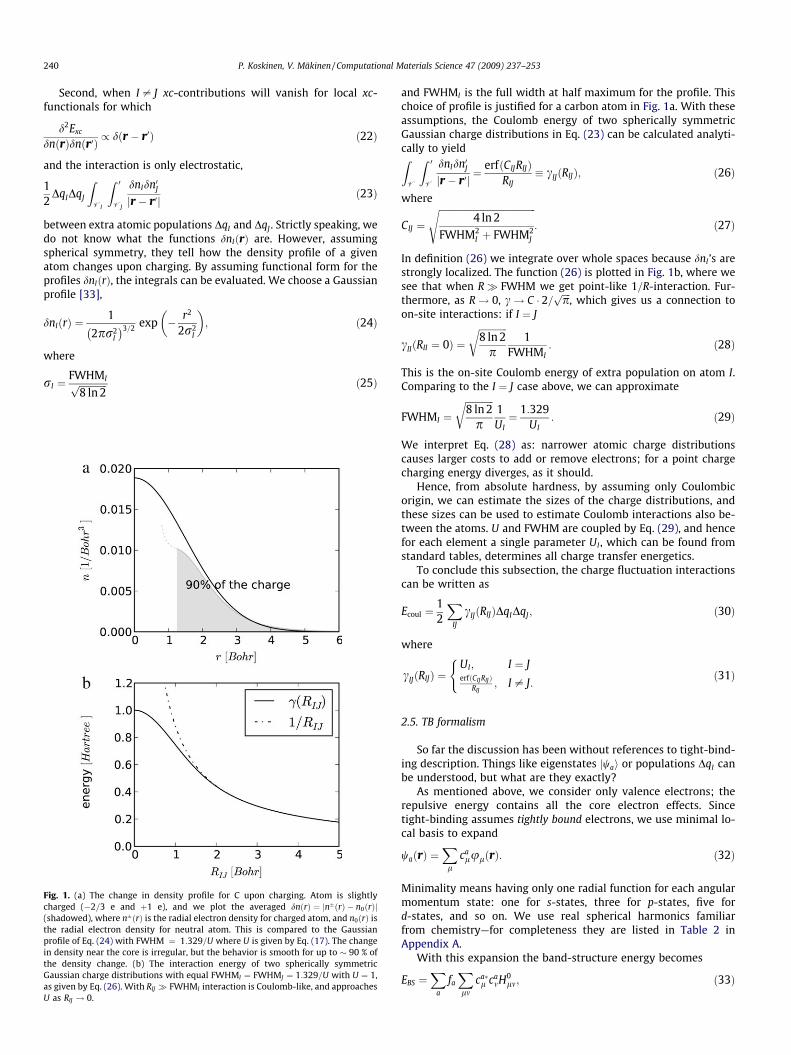
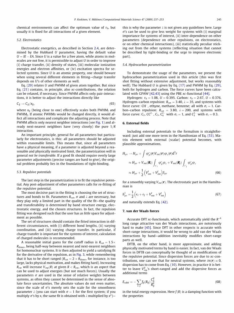
Fig. 1. (a) The change in density profile for C upon charging. Atom is slightlycharged (�2=3 e and þ1 e), and we plot the averaged dnðrÞ ¼ jnðrÞ � n0ðrÞj(shadowed), where nðrÞ is the radial electron density for charged atom, and n0ðrÞ isthe radial electron density for neutral atom. This is compared to the Gaussianprofile of Eq. (24) with FWHM ¼ 1:329=U where U is given by Eq. (17). The changein density near the core is irregular, but the behavior is smooth for up to � 90 % ofthe density change. (b) The interaction energy of two spherically symmetricGaussian charge distributions with equal FWHMI ¼ FWHMJ ¼ 1:329=U with U ¼ 1,as given by Eq. (26). With RIJ � FWHMI interaction is Coulomb-like, and approachesU as RIJ ! 0.

and FWHMI is the full width at half maximum for the profile. Thischoice of profile is justified for a carbon atom in Fig. 1a. With theseassumptions, the Coulomb energy of two spherically symmetricGaussian charge distributions in Eq. (23) can be calculated analyti-cally to yieldZV

Z 0

V

dnIdn0Jjr � r0j ¼

erfðCIJRIJÞRIJ

� cIJðRIJÞ; ð26Þ

where

CIJ ¼ffiffiffiffiffiffiffiffiffiffiffiffiffiffiffiffiffiffiffiffiffiffiffiffiffiffiffiffiffiffiffiffiffiffiffiffiffiffiffiffiffiffi

4 ln 2FWHM2

I þ FWHM2J

s: ð27Þ

In definition (26) we integrate over whole spaces because dnI ’s arestrongly localized. The function (26) is plotted in Fig. 1b, where wesee that when R� FWHM we get point-like 1=R-interaction. Fur-thermore, as R! 0, c! C � 2=

ffiffiffiffipp

, which gives us a connection toon-site interactions: if I ¼ J

cIIðRII ¼ 0Þ ¼ffiffiffiffiffiffiffiffiffiffiffiffi8 ln 2

p

r1

FWHMI: ð28Þ

This is the on-site Coulomb energy of extra population on atom I.Comparing to the I ¼ J case above, we can approximate

FWHMI ¼ffiffiffiffiffiffiffiffiffiffiffiffi8 ln 2

p

r1UI¼ 1:329

UI: ð29Þ

We interpret Eq. (28) as: narrower atomic charge distributionscauses larger costs to add or remove electrons; for a point chargecharging energy diverges, as it should.

Hence, from absolute hardness, by assuming only Coulombicorigin, we can estimate the sizes of the charge distributions, andthese sizes can be used to estimate Coulomb interactions also be-tween the atoms. U and FWHM are coupled by Eq. (29), and hencefor each element a single parameter UI , which can be found fromstandard tables, determines all charge transfer energetics.

To conclude this subsection, the charge fluctuation interactionscan be written as

Ecoul ¼12

XIJ

cIJðRIJÞDqIDqJ ; ð30Þ

where

cIJðRIJÞ ¼UI; I ¼ JerfðCIJRIJÞ

RIJ; I – J:

(ð31Þ

2.5. TB formalism

So far the discussion has been without references to tight-bind-ing description. Things like eigenstates jwai or populations DqI canbe understood, but what are they exactly?

As mentioned above, we consider only valence electrons; therepulsive energy contains all the core electron effects. Sincetight-binding assumes tightly bound electrons, we use minimal lo-cal basis to expand

waðrÞ ¼Xl

calulðrÞ: ð32Þ

Minimality means having only one radial function for each angularmomentum state: one for s-states, three for p-states, five ford-states, and so on. We use real spherical harmonics familiarfrom chemistry—for completeness they are listed in Table 2 inAppendix A.

With this expansion the band-structure energy becomes

EBS ¼X

a

fa

Xlm

cal ca

mH0lm; ð33Þ

P. Koskinen, V. Mäkinen / Computational Materials Science 47 (2009) 237–253 241

where

H0lm ¼ huljH

0jumi: ð34Þ

The tight-binding formalism is adopted by accepting the matrix ele-ments H0

lm themselves as the principal parameters of the method.This means that in tight-binding spirit the matrix elements H0

lmare just numbers. Calculation of these matrix elements is discussedin Section 3, with details left in Appendix C.

How about the atomic populations DqI? Using the localizedbasis, the total number of electrons on atom I is

qI ¼X

a

fa

ZVI

jwaðrÞj2d3r ¼

Xa

fa

Xlm

cal ca

m

ZVI

ulðrÞumðrÞd3r: ð35Þ

If neither l nor m belong to I, the integral is roughly zero, and if bothl and m belong to I, the integral is approximately dlm since orbitalson the same atom are orthonormal. If l belongs to I and m to someother atom J, the integral becomesZVI

ulðrÞumðrÞ �12

ZV

ulðrÞumðrÞ ¼12

Slm; ð36Þ

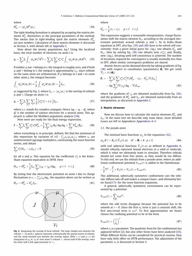
as suggested by Fig. 2, where Slm ¼ huljumi is the overlap of orbitalsl and m. Charge on atom I is

qI ¼X

a

fa

Xl2I

Xm

12

cal ca

m þ c:c:� �

Slm; ð37Þ

where c.c. stands for complex conjugate. Hence DqI ¼ qI � q0I , where

q0I is the number of valence electrons for a neutral atom. This ap-

proach is called the Mulliken population analysis [34].Now were are ready for the final energy expression,

E ¼X

a

fa

Xlm

cal ca

mH0lm þ

12

XIJ

cIJðRIJÞDqIDqJ þXI<J

VIJrepðRIJÞ; ð38Þ

where everything is, in principle, defined. We find the minimum ofthis expression by variation of dðE�

PaeahwajwaiÞ, where ea are

undetermined Lagrange multipliers, constraining the wave functionnorms, and obtainX

mcamðHlm � eaSlmÞ ¼ 0 ð39Þ

for all a and l. This equation for the coefficients cal is the Kohn–

Sham equation-equivalent in DFTB. Here

Hlm ¼ H0lm þ

12

Slm

XK

ðcIK þ cJKÞDqK ; l 2 I m 2 J: ð40Þ

By noting that the electrostatic potential on atom I due to chargefluctuations is �I ¼

PKcIKDqK , the equation above can be written as

Hlm ¼ H0lm þ h1

lmSlm; ð41Þ

Fig. 2. Integrating the overlap of local orbitals. The large shaded area denotes thevolume VI of atom I, spheres represent schematically the spatial extent of orbitals,and the small hatched area denotes the overlap region. With m 2 J and l 2 I, theintegration of ulðrÞ

umðrÞ over atom I’s volume VI misses half of the overlap, sincethe other half is left approximately to VJ .

where

h1lm ¼

12ð�I þ �JÞ; l 2 I m 2 J: ð42Þ

This expression suggests a reasonable interpretation: charge fluctu-ations shift the matrix element Hlm according to the averaged elec-trostatic potentials around orbitals l and m. As in Kohn–Shamequations in DFT, also Eqs. (39) and (40) have to be solved self-con-sistently: from a given initial guess for fDqIg one obtains h1

lm andHlm, then by solving Eq. (39) one obtains new fca

lg, and, finally,new fDqIg, iterating until self-consistency is achieved. The numberof iterations required for convergence is usually markedly less thanin DFT, albeit similar convergence problems are shared.

Atomic forces can be obtained directly by taking gradients of Eq.(38) with respect to coordinates (parameters) RI . We get (withrJ ¼ @=@RJ)

F I ¼ �X

a

fa

Xlm

cal ca

m rIH0lm � ðea � h1

lmÞrISlm

h i� DqI

XJ

ðrIcIJÞDqJ �rIErep; ð43Þ

where the gradients of cIJ are obtained analytically from Eq. (26),and the gradients of H0

lm and Slm are obtained numerically from aninterpolation, as discussed in Appendix C.

3. Matrix elements

Now we discuss how to calculate the matrix elements H0lm and

Slm. In the main text we describe only main ideas; more detailedissues are left to Appendices Appendices A–C

3.1. The pseudo-atom

The minimal basis functions ul in the expansion (32),

ulðr0Þ ¼ RlðrÞeY lðh;uÞ ðr0 ¼ RI þ r; l 2 IÞ ð44Þ

with real spherical functions eYlðh;uÞ as defined in Appendix A,should robustly represent bound electrons in a solid or molecule,which is what we ultimately want to simulate. Therefore orbitalsshould not come from free atoms, as they would be too diffuse.To this end, we use the orbitals from a pseudo-atom, where an addi-tional confinement potential V confðrÞ is added to the Hamiltonian

�12r2 � Z

rþ VHðrÞ þ VxcðrÞ þ VconfðrÞ: ð45Þ

This additional, spherically symmetric confinement cuts the orbi-tals’ diffuse tails off and makes a compact basis—and ultimately bet-ter basis[17]—for the wave function expansion.

A general, spherically symmetric environment can be repre-sented by a potential

VconfðrÞ ¼X1i¼0

v2ir2i; ð46Þ

where the odd terms disappear because the potential has to besmooth at r ¼ 0. Since the first v0 term is just a constant shift, thefirst non-trivial term is v2r2. To first approximation we hencechoose the confining potential to be of the form

VconfðrÞ ¼rr0

� �2

; ð47Þ

where r0 is a parameter. The quadratic form for the confinement hasappeared before [2], but also other forms have been analyzed [35].While different forms can be considered for practical reasons, theyhave only little effect on DFTB performance. The adjustment of theparameter r0 is discussed in Section 5.

242 P. Koskinen, V. Mäkinen / Computational Materials Science 47 (2009) 237–253

The pseudo-atom is calculated with DFT only once for a givenconfining potential. This way we get ul’s (more precisely, Rl’s),the localized basis functions, for later use in matrix elementcalculations.

One technical detail we want to point out here concerns orbitalconventions. Namely, once the orbitals ul are calculated, their signand other conventions should never change. Fixed conventionshould be used in all simultaneously used Slater–Koster tables;using different conventions for same elements gives inconsistenttables that are plain nonsense. The details of our conventions,along with other technical details of the pseudo-atom calculations,are discussed in Appendix A.

3.2. Overlap matrix elements

Using the orbitals from pseudo-atom calculations, we need tocalculate the overlap matrix elements

Slm ¼Z

ulðrÞumðrÞd

3r: ð48Þ

Since orbitals are chosen real, the overlap matrix is real andsymmetric.

The integral with ul at RI and um at RJ can be calculated alsowith ul at the origin and um at RIJ . Overlap will hence depend onRIJ , or equivalently, on RIJ and bRIJ separately. Fortunately, thedependence on bRIJ is fully governed by Slater–Koster transformationrules [36]. Only one to three Slater–Koster integrals, depending onthe angular momenta of ul and um, are needed to calculate theintegral with any bRIJ for fixed RIJ . These rules originate from theproperties of spherical harmonics.

The procedure is hence the following: we integrate numericallythe required Slater–Koster integrals for a set of RIJ , and store themin a table. This is done once for all orbital pairs. Then, for a givenorbital pair, we interpolate this table for RIJ , and use the Slater–Koster rules to get the overlap with any geometry—fast andaccurately.

Readers unfamiliar with the Slater–Koster transformations canread the detailed discussion in Appendix B. The numerical integra-tion of the integrals is discussed in Appendix C.

Before concluding this subsection, we make few remarks aboutnon-orthogonality. In DFTB it originates naturally and inevitablyfrom Eq. (48), because non-overlapping orbitals with diagonaloverlap matrix would yield also diagonal Hamiltonian matrix,which would mean chemically non-interacting system. Thetransferability of a tight-binding model is often attributed tonon-orthogonality, because it accounts for the spatial nature ofthe orbitals more realistically.

Non-orthogonality requires solving a generalized eigenvalueproblem, which is more demanding than normal eigenvalue prob-lem. Non-orthogonality complicates, for instance, also gauge trans-formations, because the phase from the transformations is not welldefined for the orbitals due to overlap. The Peierls substitution[37], while gauge invariant in orthogonal tight-binding [38,39], isnot gauge invariant in non-orthogonal tight-binding (but affectsonly time-dependent formulation).

3.3. Hamiltonian matrix elements

From Eq. (34) the Hamiltonian matrix elements are

H0lm ¼

ZulðrÞ

�12r2 þ Vs½n0�ðrÞ

� �umðrÞ; ð49Þ

where

Vs½n0�ðrÞ ¼ VextðrÞ þ VH½n0�ðrÞ þ Vxc½n0�ðrÞ ð50Þ

is the effective potential evaluated at the (artificial) neutral densityn0ðrÞ of the system. The density n0 is determined by the atoms inthe system, and the above matrix element between basis states land m, in principle, depends on the positions of all atoms. However,since the integrand is a product of factors with three centers, twowave functions and one potential (and kinetic), all of which arenon-zero in small spatial regions only, reasonable approximationscan be made.

First, for diagonal elements Hll one can make a one-centerapproximation where the effective potential within volume VI is

Vs½n0�ðrÞ � Vs;I½n0;I�ðrÞ; ð51Þ

where l 2 I. This integral is approximately equal to the eigenener-gies el of free atom orbitals. This is only approximately correct sincethe orbitals ul are from the confined atom, but is a reasonableapproximation that ensures the correct limit for free atoms.

Second, for off-diagonal elements we make the two-centerapproximation: if l is localized around atom I and m is localizedaround atom J, the integrand is large when the potential is local-ized either around I or J as well; we assume that the crystal fieldcontribution from other atoms, when the integrand has three dif-ferent localized centers, is small. Using this approximation theeffective potential within volume VI þVJ becomes

Vs½n0�ðrÞ � Vs;I½n0;I�ðrÞ þ Vs;J ½n0;J �ðrÞ; ð52Þ

where Vs;I½n0;I�ðrÞ is the Kohn-Sham potential with the density of aneutral atom. The Hamiltonian matrix element is

H0lm ¼

ZulðrÞ

�12r2 þ Vs;IðrÞ þ Vs;JðrÞ

� �umðrÞ; ð53Þ

where l 2 I and m 2 J. Prior to calculating the integral, we have toapply the Hamiltonian to um. But in other respects the calculationis similar to overlap matrix elements: Slater–Koster transforma-tions apply, and only a few integrals have to be calculated numeri-cally for each pair of orbitals, and stored in tables for futurereference. See Appendix C.2 for details of numerical integration ofthe Hamiltonian matrix elements.

4. Fitting the repulsive potential

In this section we present a systematic approach to fit the repul-sive functions VIJ

repðRIJÞ that appear in Eq. (38)—and a systematicway to describe the fitting. But first we discuss some difficulties re-lated to the fitting process.

The first and straightforward way of fitting is simple: calculatedimer curve EDFTðRÞ for the element pair with DFT, requireEDFTðRÞ ¼ EDFTBðRÞ, and solve

V repðRÞ ¼ EDFTðRÞ � EBSðRÞ þ EcoulðRÞ½ �: ð54Þ

We could use also other symmetric structures with N bonds havingequal RIJ ¼ R, and require

N � V repðRÞ ¼ EDFTðRÞ � EBSðRÞ þ EcoulðRÞ½ �: ð55Þ

In practice, unfortunately, it does not work out. The approximationsmade in DFTB are too crude, and hence a single system is insuffi-cient to provide a robust repulsion. As a result, fitting repulsivepotentials is difficult task, and forms the most laborous part ofparametrizing in DFTB.

Let us compare things with DFT. As mentioned earlier, we triedto dump most of the difficult physics into the repulsive potential,and hence V rep in DFTB has practical similarity to Exc in DFT. InDFTB, however, we have to make a new repulsion for each pairof atoms, so the testing and fitting labor compared to DFT function-als is multifold. Because xc-functionals in DFT are well docu-mented, DFT calculations of a reasonably documented article can

P. Koskinen, V. Mäkinen / Computational Materials Science 47 (2009) 237–253 243

be reproduced, whereas reproducing DFTB calculations is usuallyharder. Even if the repulsive functions are published, it would bea great advantage to be able to precisely describe the fitting pro-cess; repulsions could be more easily improved upon.

Our starting point is a set of DFT structures, with geometries R,energies EDFTðRÞ, and forces FDFT (zero for optimized structures). Anatural approach would be to fit V rep so that energies EDFTBðRÞ andforces FDFTB are as close to DFT ones as possible. In other words, wewant to minimize force differences F DFT � FDFTB

and energy dif-ferences EDFT � EDFTBj j on average for the set of structures. Thereare also other properties such as basis set quality (large overlapwith DFT and DFTB wave functions), energy spectrum (similarityof DFT and DFTB density of states), or charge transfer to be com-pared with DFT, but these originate already from the electronicpart, and should be modified by adjusting V confðrÞ and HubbardU. Repulsion fitting is always the last step in the parametrizing,and affects only energies and forces.

In practice we shall minimize, however, only force differ-ences—we fit repulsion derivative, not repulsion directly. The fit-ting parameters, introduced shortly, can be adjusted to get energydifferences qualitatively right, but only forces are used in thepractical fitting algorithm. There are several reasons for this. First,forces are absolute, energies only relative. For instance, since wedo not consider spin, it is ambiguous whether to fit to DFT dimercurve with spin-polarized or spin-paired free atom energies. Wecould think that lower-level spin-paired DFT is the best DFTBcan do, so we compare to spin-paired dimer curve—but we shouldfit to energetics of nature, not energetics in some flavors of DFT.Second, for faithful dynamics it is necessary to have right forcesand right geometries of local energy minima; it is more importantfirst to get local properties right, and afterwards look how theglobal properties, such as energy ordering of different structuralmotifs, come out. Third, the energy in DFTB comes mostly fromthe band-structure part, not repulsion. This means that if alreadythe band-structure part describes energy wrong, the short-rangedrepulsions cannot make things right. For instance, if EDFTðRÞ andEDFTBðRÞ for dimer deviates already with large R, short-rangerepulsion cannot cure the energetics anymore. For transferabilityrepulsion has to be monotonic and smooth, and if repulsion is ad-justed too rapidly catch up with DFT energetics, the forces will gowrong.

For the set of DFT structures, we will hence minimize DFT andDFTB force differences, using the recipes below.

4.1. Collecting data

To fit the derivative of the repulsion for element pair AB, weneed a set of data points fRi;V

0repðRiÞg. As mentioned before, fitting

to dimer curve alone does not give a robust repulsion, because thesame curve is supposed to work in different chemical environ-ments. Therefore it is necessary to collect the data points from sev-eral structures, to get a representative average over different typesof chemical bonds. Here we present examples on how to acquiredata points.

4.1.1. Force curves and equilibrium systemsThis method can be applied to any system where all the bond

lengths between the elements equal RAB or otherwise are beyondthe selected cutoff radius Rcut. In other words, the only energy com-ponent missing from these systems is the repulsion from N bondsbetween elements A and B with matching bond lengths. Hence,

EDFTBðRABÞ ¼ EBSðRABÞ þ EcoulðRABÞ þ eErep þ N � V repðRABÞ; ð56Þ

where eErep is the repulsive energy independent of RAB. This setupallows us to change RAB, and we will require

V 0repðRABÞ ¼E0DFTðRABÞ � E0BSðRABÞ þ E0coulðRABÞ

�N

; ð57Þ

where the prime stands for a derivative with respect to RAB. The eas-iest way is first to calculate the energy curve and use finite differ-ences for derivatives. In fact, systems treated this way can haveeven different RAB’s if only the ones that are equal are chosen to vary(e.g. a complex system with one appropriate AB bond on its surface).For each system, this gives a family of data points for the fitting; thenumber of points in the family does not affect fitting, as explainedlater. The dimer curve, with N ¼ 1, is clearly one system where thismethod can be applied. For any equilibrium DFT structure thingssimplify into

V 0rep R0AB

� �¼�E0BS R0

AB

� �� E0coul R0

AB

� �N

; ð58Þ

where R0AB is the distance for which E0DFT R0

AB

� �¼ 0.

4.1.2. Homonuclear systemsIf a cluster or a solid has different bond lengths, the energy

curve method above cannot be applied (unless a subset of bondsare selected). But if the system is homonuclear, the data pointscan be obtained the following way. The force on atom I is

F I ¼ F0I þ

XJ–I

V 0repðRIJÞbRIJ ð59Þ

¼ F0I þ

XJ–I

�IJbRIJ; ð60Þ

where F0I is the force without repulsions. Then we minimize the

sumXI

FDFT;I � F I

2 ð61Þ

with respect to �IJ , with �IJ ¼ 0 for pair distances larger than the cut-off. The minimization gives optimum �IJ , which can be used directly,together with their RIJ ’s, as another family of data points in thefitting.

4.1.3. Other algorithmsFitting algorithms like the ones above are easy to construct, but

a few general guidelines are good to keep in mind.While pseudo-atomic orbitals are calculated with LDA-DFT, the

systems to fit the repulsive potential should be state-of-the-art cal-culations; all structural tendencies—whether right or wrong—aredirectly inherited by DFTB. Even reliable experimental structurescan be used as fitting structures; there is no need to think DFTBshould be parametrized only from theory. DFTB will not becomeany less density-functional by doing so.

As data points are calculated by stretching selected bonds (orcalculating static forces), also other bonds may stretch (dimer isone exception). These other bonds should be large enough to ex-clude repulsive interactions; otherwise fitting a repulsion betweentwo elements may depend on repulsion between some other ele-ment pairs. While this is not illegal, the fitting process easily be-comes complicated. Sometimes the stretching can affect chemicalinteractions between elements not involved in the fitting; this isworth avoiding, but sometimes it may be inevitable.

4.2. Fitting the repulsive potential

Transferability requires the repulsion to be short-ranged, andwe choose a cutoff radius Rcut for which V repðRcutÞ ¼ 0, and alsoV 0repðRcutÞ ¼ 0 for continuous forces. Rcut is one of the mainparameters in the fitting process. Then, with given Rcut, after having

244 P. Koskinen, V. Mäkinen / Computational Materials Science 47 (2009) 237–253

collected enough data points fRi;V0rep;ig, we can fit the function

V 0repðRÞ. The repulsion itself is

V repðRÞ ¼ �Z Rcut

RV 0repðrÞdr: ð62Þ

Fitting of V 0rep using the recipe below provides a robust andunbiased fit to the given set of points, and the process is easy tocontrol. We choose a standard smoothing spline [40] forV 0repðRÞ � UðRÞ, i.e. we minimize the functional

S UðRÞ½ � ¼XM

i¼1

V 0rep;i � UðRiÞri

!2

þ kZ Rcut

U00ðRÞ2dR ð63Þ

for total M data points fRi;V0rep;ig, where UðRÞ is given by a cubic

spline. Spline gives an unbiased representation for UðRÞ, and thesmoothness can be directly controlled by the parameter k. Large kmeans expensive curvature and results in linear UðRÞ (quadraticV rep) going through the data points only approximately, while smallk considers curvature cheap and may result in a wiggled UðRÞ pass-ing through the data points exactly. The parameter k is the secondparameter in the fitting process. Other choices for UðRÞ can be used,such as low-order polynomials [2], but they sometimes behave sur-prisingly while continuously tuning Rcut. For transferability thebehavior of the derivative should be as smooth as possible, prefer-ably also monotonous (the example in Fig. 3a is slightly non-monot-onous and should be improved upon).

The parameters ri are the data point uncertainties, and can beused to weight systems differently. With the dimension of force,ri’s have also an intuitive meaning as force uncertainties, thelengths of force error bars. As described above, each system mayproduce a family of data points. We would like, however, the fitting

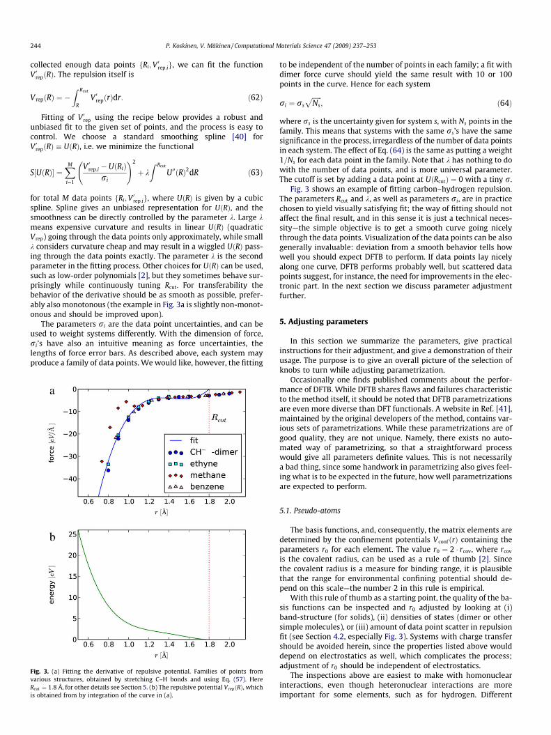
Fig. 3. (a) Fitting the derivative of repulsive potential. Families of points fromvarious structures, obtained by stretching C–H bonds and using Eq. (57). HereRcut ¼ 1:8 Å, for other details see Section 5. (b) The repulsive potential V repðRÞ, whichis obtained from by integration of the curve in (a).

to be independent of the number of points in each family; a fit withdimer force curve should yield the same result with 10 or 100points in the curve. Hence for each system

ri ¼ rs

ffiffiffiffiffiffiNs

p; ð64Þ

where rs is the uncertainty given for system s, with Ns points in thefamily. This means that systems with the same rs’s have the samesignificance in the process, irregardless of the number of data pointsin each system. The effect of Eq. (64) is the same as putting a weight1=Ns for each data point in the family. Note that k has nothing to dowith the number of data points, and is more universal parameter.The cutoff is set by adding a data point at UðRcutÞ ¼ 0 with a tiny r.

Fig. 3 shows an example of fitting carbon–hydrogen repulsion.The parameters Rcut and k, as well as parameters ri, are in practicechosen to yield visually satisfying fit; the way of fitting should notaffect the final result, and in this sense it is just a technical neces-sity—the simple objective is to get a smooth curve going nicelythrough the data points. Visualization of the data points can be alsogenerally invaluable: deviation from a smooth behavior tells howwell you should expect DFTB to perform. If data points lay nicelyalong one curve, DFTB performs probably well, but scattered datapoints suggest, for instance, the need for improvements in the elec-tronic part. In the next section we discuss parameter adjustmentfurther.

5. Adjusting parameters

In this section we summarize the parameters, give practicalinstructions for their adjustment, and give a demonstration of theirusage. The purpose is to give an overall picture of the selection ofknobs to turn while adjusting parametrization.

Occasionally one finds published comments about the perfor-mance of DFTB. While DFTB shares flaws and failures characteristicto the method itself, it should be noted that DFTB parametrizationsare even more diverse than DFT functionals. A website in Ref. [41],maintained by the original developers of the method, contains var-ious sets of parametrizations. While these parametrizations are ofgood quality, they are not unique. Namely, there exists no auto-mated way of parametrizing, so that a straightforward processwould give all parameters definite values. This is not necessarilya bad thing, since some handwork in parametrizing also gives feel-ing what is to be expected in the future, how well parametrizationsare expected to perform.

5.1. Pseudo-atoms

The basis functions, and, consequently, the matrix elements aredetermined by the confinement potentials VconfðrÞ containing theparameters r0 for each element. The value r0 ¼ 2 � rcov, where rcov

is the covalent radius, can be used as a rule of thumb [2]. Sincethe covalent radius is a measure for binding range, it is plausiblethat the range for environmental confining potential should de-pend on this scale—the number 2 in this rule is empirical.

With this rule of thumb as a starting point, the quality of the ba-sis functions can be inspected and r0 adjusted by looking at (i)band-structure (for solids), (ii) densities of states (dimer or othersimple molecules), or (iii) amount of data point scatter in repulsionfit (see Section 4.2, especially Fig. 3). Systems with charge transfershould be avoided herein, since the properties listed above woulddepend on electrostatics as well, which complicates the process;adjustment of r0 should be independent of electrostatics.

The inspections above are easiest to make with homonuclearinteractions, even though heteronuclear interactions are moreimportant for some elements, such as for hydrogen. Different

P. Koskinen, V. Mäkinen / Computational Materials Science 47 (2009) 237–253 245

chemical environments can affect the optimum value of r0, butusually it is fixed for all interactions of a given element.

5.2. Electrostatics

Electrostatic energetics, as described in Section 2.4, are deter-mined by the Hubbard U parameter, having the default valueU ¼ IE� EA. Since U is a value for a free atom, while atoms in mol-ecules are not free, it is permissible to adjust U in order to improve(i) charge transfer, (ii) density of states, (iii) molecular ionizationenergies and electron affinities, or (iv) excitation spectra for se-lected systems. Since U is an atomic property, one should bewarewhen using several different elements in fitting—charge transferdepends on U’s of other elements as well.

Eq. (29) relates U and FWHM of given atom together. But sinceEq. (21) contains, in principle, also xc-contributions, the relationcan be relaxed, if necessary. Since FWHM affects only pair-interac-tions, it is better to adjust the interactions directly like

CIJ ! CIJ=xIJ; ð65Þ

where xIJ (being close to one) effectively scales both FWHMI andFWHMJ . If atomic FWHMs would be changed directly, it would af-fect all interactions and complicate the adjusting process. Note thatFWHM affects only nearest neighbor interactions (see Fig. 1) and al-ready next-nearest neighbors have (very closely) the pure 1=Rinteraction.

An important principle, general for all parameters but particu-larly for electrostatics, is this: all parameters should be adjustedwithin reasonable limits. This means that, since all parametershave a physical meaning, if a parameter is adjusted beyond a rea-sonable and physically motivated limit, the parametrization will ingeneral not be transferable. If a good fit should require overly largeparameter adjustments (precise ranges are hard to give), the origi-nal problem probably lies in the foundations of tight-binding.

5.3. Repulsive potentials

The last step in the parametrization is to fit the repulsive poten-tial. Any post-adjustment of other parameters calls for re-fitting ofthe repulsive potential.

The most decisive part in the fitting is choosing the set of struc-tures and bonds to fit. Parameters Rcut, r and k are necessary, butthey play only a limited part in the quality of the fit—the qualityand transferability is determined by band structure energy, elec-trostatic energy, and the chosen structures. In fact, the repulsionfitting was designed such that the user has as little space for adjust-ment as possible.

The set of structures should contain the fitted interaction in dif-ferent circumstances, with (i) different bond lengths, (ii) varyingcoordination, and (iii) varying charge transfer. In particular, ifcharge transfer is important for the systems of interest, calculationof charged molecules is recommended.

A reasonable initial guess for the cutoff radius is Rcut ¼ 1:5�Rdimer, being half-way between nearest and next-nearest neighborsfor homonuclear systems. It is then adjusted to yield a satisfying fitfor the derivative of the repulsion, as in Fig. 3, while rememberingthat it has to be short ranged (Rcut ¼ 2� Rdimer, for instance, is toolarge, lacks physical motivation, and makes fitting hard). IncreasingRcut will increase V repðRÞ at given R < Rcut, which is an aspect thatcan be used to adjust energies (but not much forces). Usually theparameters r are used in the sense of relative weights betweensystems, as often they cannot be determined in the sense of abso-lute force uncertainties. The absolute values do not even matter,since the scale of r’s merely sets the scale for the smoothnessparameter k (you can start with r ¼ 1 for the first system; if youmultiply r’s by x, the same fit is obtained with k multiplied by x2)—

this is why the parameter k is not given any guidelines here. Larger’s can be used to give less weight for systems with (i) marginalimportance for systems of interest, (ii) inter-dependence on otherparameters (dependence on other repulsions, on electrostatics,or on other chemical interactions), (iii) statistically peculiar stick-ing out from the other systems (reflecting situation that cannotbe described by tight-binding or the urge to improve electronicpart).

5.4. Hydrocarbon parametrization

To demonstrate the usage of the parameters, we present thehydrocarbon parametrization used in this article (this was firstshot fitting without extensive adjustment, but works reasonablywell). The Hubbard U is given by Eq. (17) and FWHM by Eq. (29),both for hydrogen and carbon. The force curves have been calcu-lated with GPAW [42,43] using the PBE xc-functional [44].

Hydrogen: r0 ¼ 1:08, U ¼ 0:395. Carbon: r0 ¼ 2:67, U ¼ 0:376.Hydrogen–carbon repulsion: Rcut ¼ 3:40, k ¼ 35, and systems withforce curve: CH�, ethyne, methane, benzene; all with ri ¼ 1. Car-bon–carbon repulsion: Rcut ¼ 3:80, k ¼ 200, and systems withforce curve: C2, CC2�, C3, C2�

4 with ri ¼ 1, and C2�3 with ri ¼ 0:3.

6. External fields

Including external potentials to the formalism is straightfor-ward: just add one more term in the Hamiltonian of Eq. (53). Ma-trix element with external (scalar) potential becomes, withplausible approximations,

Hlm ! Hlm þZ

ulðrÞVextðrÞumðrÞd3r

� Hlm þ VextðRIÞZVI

ulum þ VextðRJÞZVJ

ulum

� Hlm þ12

VIext þ VJ

ext

� �Slm ð66Þ

for a smoothly varying VextðrÞ. The electrostatic part in the Hamilto-nian is

h1lm ¼

12�I þ �J þ VI

ext þ VJext

� �ð67Þ

and naturally extends Eq. (42).

7. van der Waals forces

Accurate DFT xc-functionals, which automatically yield the R�6

long range attractive van der Waals interactions, are notoriouslyhard to make [45]. Since DFT in other respects is accurate withshort-range interactions, it would be wrong to add van der Waalsinteractions by hand—addition inevitably modifies short-rangeparts as well.

DFTB, on the other hand, is more approximate, and addingphysically motivated terms by hand is easier. In fact, van der Waalsforces in DFTB can conceptually be thought of as modifications ofthe repulsive potential. Since dispersion forces are due to xc-con-tributions, one can see that for neutral systems, where dnðrÞ � 0,dispersion has to come from Eq. (10). However, in practice it is bet-ter to leave VIJ

rep’s short-ranged and add the dispersive forces asadditional terms

EvdW ¼ �XI<J

fIJðRIJÞCIJ

6

R6IJ

ð68Þ

in the total energy expression. Here f ðRÞ is a damping function withthe properties

246 P. Koskinen, V. Mäkinen / Computational Materials Science 47 (2009) 237–253

f ðRÞ ¼� 1; R J R0

� 0; R K R0;

�ð69Þ

because the idea is to switch off van der Waals interactions for dis-tances smaller than R0, a characteristic distance where chemicalinteractions begin to emerge.

The C6-parameters depend mainly on atomic polarizabilitiesand have nothing to do with DFTB formalism. Care is required toavoid large repulsive forces, coming from abrupt behavior in f ðRÞnear R � R0, which could result in local energy minima. For a de-tailed descriptions about the C6-parameters and the form of f ðRÞwe refer to original Refs. [46,47]; in this section we merely demon-strate how straightforward it is, in principle, to include van derWaals forces in DFTB.

8. Periodic boundary conditions

8.1. Bravais lattices

Calculation of isolated molecules with DFTB is straightforward,but implementation of periodic boundary conditions and calcula-tion of electronic band-structures is also easy[48]. As mentionedin the introduction, this is usually the first encounter with tight-binding models for most physicists; our choice was to discuss peri-odic systems at later stage.

In a crystal periodic in translations T , the wave functions havethe Bloch form

waðk; rÞ ¼ eik�ruaðk; rÞ; ð70Þ

where uaðk; rÞ is function with crystal periodicity [49]. This meansthat a wave function waðk; rÞ changes by a phase eik�T in translationT . We define new basis functions, not as localized orbitals anymore,but as Bloch waves extended throughout the whole crystal

ulðk; rÞ ¼1ffiffiffiffiNp

XT

eik�Tulðr � TÞ; ð71Þ

where N is the (infinite) number of unit cells in the crystal. Theeigenfunction ansatz

waðk; rÞ ¼Xl

calðkÞulðk; rÞ ð72Þ

is then also an extended Bloch wave, as required by Bloch theorem,because k is the same for all basis states. Matrix elements in thisnew basis are

Slmðk;k0Þ ¼ dðk� k0ÞSlmðkÞ ð73Þ

and

Hlmðk;k0Þ ¼ dðk� k0ÞHlmðkÞ; ð74Þ

where

SlmðkÞ ¼X

T

eik�TZ

ulðrÞumðr � TÞ� �

�X

T

eik�T SlmðTÞ ð75Þ

and similarly for H. Obviously the Hamiltonian conserves k—that iswhy k labels the eigenstates in the first place. Note that the new ba-sis functions are usually not normalized.

Inserting the trial wave function (72) into Eq. (38) and by usingthe variational principle we obtain the secular equationX

mcamðkÞ HlmðkÞ � eaðkÞSlmðkÞ

�¼ 0; ð76Þ

where

HlmðkÞ ¼ H0lmðkÞ þ h1

lmSlmðkÞ ð77Þ

for each k-point from a chosen set, such as Monkhorst–Pack sam-pled [50]. Above we have

h1lm ¼

12ð�I þ �JÞ l 2 I; m 2 J; ð78Þ

as in Eq. (42), and Mulliken charges are extensions of Eq. (37),

qI ¼X

a

Xk

faðkÞXl2I;m

12

cal ðkÞca

mðkÞSlmðkÞ þ c:c:h i

: ð79Þ

The sum for the electrostatic energy per unit cell,

Ecoul ¼12

Xunit cell

IJ

XT

cIJðRIJ � TÞDqIDqJ ; ð80Þ

can be calculated with standard methods, such as Ewald summation[51], and the repulsive part,

XI<J

V IJrepðRIJÞ ¼

12

Xunit cell

IJ

XT

VIJrepðRIJ � TÞ ð81Þ

is easy because repulsions are short-ranged (and V repð0Þ ¼ 0 isunderstood).

8.2. General symmetries

Thanks to the transparent formalism of DFTB, it is easy to con-struct more flexible boundary conditions, such as the ‘‘wedgeboundary condition” introduced in Ref. [52]. This is one exampleof DFTB in method development.

General triclinic unit cells are copied by translations, and DFTimplementation is easy with plane waves, real-space grids or local-ized orbitals with fixed quantization axis. But if we allow the quan-tization axis of localized orbitals to be position-dependent, we cantreat more general symmetries which have rotational symmetry[53] or even combined rotational and translational (chiral) symme-tries [54].

The basic idea is to enforce the orbitals to have the the samesymmetry as the system. This requires that basis functions not onlydepend on atom positions like

ulðr � RlÞ; ð82Þ

as usual, but more generally like

DðRlÞulðrÞ; ð83Þ

where DðRlÞ is an operator transforming the orbitals in any posi-tion-dependent manner, including both translations and rotations.The only requirement is that the orbitals are complete and ortho-normal for a given angular momentum. If the quantization axeschange, things become unfortunately messy. However, suitably de-fined basis orbitals yield well-defined Hamiltonian and overlapmatrices, and enable simulations of systems like bent tubes or slabs,helical structures such as DNA, or a piece of spherical surface—witha greatly reduced number of atoms. Similar concepts are familiarfrom chemistry, where symmetry-adapted molecular orbitals areconstructed from the atomic orbitals, and computational effort ishereby reduced [55]. Detailed treatment of these general symme-tries is a work in progress [56].

9. Density-matrix formulation

In this section we introduce DFTB using density-matrix formu-lation. We do this because not only does the formulation simplifyexpressions, but it also makes calculations faster in practice. Thispractical advantage comes because the density-matrix,

P. Koskinen, V. Mäkinen / Computational Materials Science 47 (2009) 237–253 247

qlm ¼X

a

faðcalca

m Þ ¼X

a

faðqalmÞ; ð84Þ

contains a loop over eigenstates; quantities calculated with qlm sim-ply avoid this extra loop. It has the properties

qSq ¼ q ð� idempotencyÞ; ð85Þqlm ¼ qml ðq ¼ qyÞ; ð86ÞTrðqaSÞ ¼ 1 ðeigenfunction normalizationÞ: ð87Þ

We define also the energy-weighted density-matrix

qelm ¼

Xa

eafacalca

m ; ð88Þ

and symmetrized density matrix

~qlm ¼12ðqlm þ qlmÞ; ð89Þ

which is symmetric and real. Using qlm we obtain simple expres-sions, for example, for

EBS ¼ TrðqH0Þ ð90ÞNel ¼ Trð~qSÞ ¼

Xl

Xm

~qlmSml; ð91Þ

qI ¼ TrIð~qSÞ ¼Xl2I

Xm

~qlmSml; ð92Þ

where EBS is the band-structure energy, Nel is the total number ofelectrons, and qI is the Mulliken population on atom I. TrI is partialtrace over orbitals of atom I alone.

It is practical to define also matrices’ gradients. They do not di-rectly relate to density matrix formulation, but equally simplifynotation, and are useful in practical implementations. We define(with rJ ¼ @=@RJ)

dSlm ¼ rJSlm ðl 2 I; m 2 JÞ

�Z

ulðr � RIÞrJumðr � RJÞ ¼ huljrJumi ð93Þ

and

dHlm ¼ rJHlmhuljHjrJumi ðl 2 I; m 2 JÞ ð94Þ

with the properties dSlm ¼ �dSml and dHlm ¼ �dHml. From thesedefinitions we can calculate analytically, for instance, the timederivative of the overlap matrix for a system in motion_S ¼ ½dS;V � ð95Þ

with commutator ½A;B� and matrix Vlm ¼ dlm_RI , l 2 I. Force from the

band-energy part, the first line in Eq. (43), for atom I can be ex-pressed as

F I ¼ �TrIðqdH � qedSÞ þ c:c:; ð96Þ

which is, besides compact, useful in implementation. The density-matrix formulation introduced here is particularly useful in elec-tronic structure analysis, discussed in the following section.

10. Simplistic electronic structure analysis

One great benefit of tight-binding is the ease in analyzing theelectronic structure. In this section we present selected analysistools, some old and renowned, others casual but intuitive. Othersimple tools for chemical analysis of bonding can be found fromRef. [57].

10.1. Partial Mulliken populations

The Mulliken population on atom I,

qI ¼ TrIð~qSÞ ¼Xl2I

Xm

~qlmSml ¼Xl2I

ð~qSÞll ð97Þ

is easy to partition into smaller pieces. Population of a single orbitall is

qðlÞ ¼X

m

~qlmSml ¼ ð~qSÞll; ð98Þ

while population on atom I due to eigenstate wa alone is

qI;a ¼ TrIð~qaSÞ ¼Xl2I

Xm

~qalmSml; ð99Þ

so thatXI

Xa

faqI;a

!¼X

I

ðqIÞ ¼ Nel: ð100Þ

Population on orbitals of atom I with angular momentum l is,similarly,

qlI ¼

Xl2Iðll¼lÞ

ð~qSÞll: ð101Þ

The partial Mulliken populations introduced above are simple, butenable surprisingly rich analysis of the electronic structure, as dem-onstrated below.

10.2. Analysis beyond Mulliken charges

At this point, after discussing Mulliken population analysis, wecomment on the role of wave functions in DFTB. Namely, internallyDFTB formalism uses atom resolution for any quantity, and thetight-binding spirit means that the matrix elements Hlm and Slm

are just parameters, nothing more. Nonetheless, the elements Hlm

and Slm are obtained from genuine basis orbitals ulðrÞ usingwell-defined procedure—these basis orbitals remain constantlyavailable for deeper analysis. The wave functions are

waðrÞ ¼Xl

calulðrÞ ð102Þ

and the total electron density is

nðrÞ ¼X

a

fajwðrÞj2 ¼Xlm

qlmumðrÞulðrÞ; ð103Þ

awaiting for inspection with tools familiar from DFT. One should,however, use the wave functions only for analysis[58]. The formal-ism itself is better off with Mulliken charges. But for visualizationand for gaining understanding this is a useful possibility. This dis-tinguishes DFTB from semiempirical methods, which—in princi-ple—do not possess wave functions but only matrix elements(unless made ad hoc by hand).

10.3. Densities of states

Mulliken populations provide intuitive tools to inspect elec-tronic structure. Let us first break down the energy spectrum intovarious components. The complete energy spectrum is given by thedensity of states (DOS),

DOSðeÞ ¼X

a

drðe� eaÞ; ð104Þ

where drðeÞ can be either the peaked Dirac delta-function, or somefunction—such as a Gaussian or a Lorentzian—with broadeningparameter r. DOS carrying spatial information is the local densityof states,

LDOSðe; rÞ ¼X

a

drðe� eaÞjwaðrÞj2 ð105Þ

with integration overR

d3r yielding DOSðeÞ. Sometimes it is definedas

248 P. Koskinen, V. Mäkinen / Computational Materials Science 47 (2009) 237–253

LDOSðrÞ ¼X

a

f 0ajwaðrÞj2; ð106Þ

where f 0a are weights chosen to select states with given energies, asin scanning tunneling microscopy simulations[59]. Mullikencharges, pertinent to DFTB, yield LDOS with atom resolution,

LDOSðe; IÞ ¼X

a

drðe� eaÞqI;a; ð107Þ

which can be used to project density for group of atoms R as

LDOSRðeÞ ¼XI2R

LDOSðe; IÞ: ð108Þ

For instance, if systems consists of surface and adsorbed molecule,we can plot LDOSmolðeÞ and LDOSsurfðeÞ to see how states are distrib-uted; naturally LDOSmolðeÞ þ LDOSsurfðeÞ ¼ LDOSðeÞ.

Similar recipes apply for projected density of states, where DOSis broken into angular momentum components,

PDOSðe; lÞ ¼X

a

drðe� eaÞX

I

qlI;a; ð109Þ

such that, againP

lPDOSðe; lÞ ¼ DOSðeÞ.

10.4. Mayer bond-order

Bond strengths between atoms are invaluable chemical infor-mation. Bond order is a dimensionless number attached to thebond between two atoms, counting the differences of electronpairs on bonding and antibonding orbitals; ideally it is one for sin-gle, two for double, and three for triple bonds. In principle, anybond strength measure is equally arbitrary; in practice, some mea-sures are better than others. A measure suitable for many purposesin DFTB is Mayer bond-order [57], defined for bond IJ as

MIJ ¼X

l2I;m2J

ð~qSÞlmð~qSÞml: ð110Þ

The off-diagonal elements of ~qS can be understood as Mullikenoverlap populations, counting the number of electrons in the over-lap region—the bonding region. It is straightforward, if necessary, topartition Eq. (110) into pieces, for inspecting angular momenta oreigenstate contributions in bonding. Look at Refs. [60,57] for furtherdetails, and Table 1 for examples of usage.

10.5. Covalent bond energy

Another useful bonding measure is the covalent bond energy,which is not just a dimensionless number but measures bondingdirectly using energy [61].

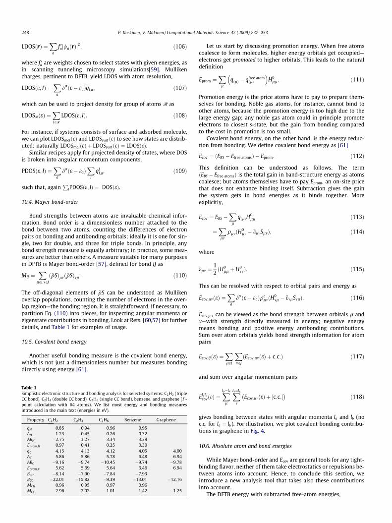
Table 1Simplistic electronic structure and bonding analysis for selected systems: C2H2 (tripleCC bond), C2H4 (double CC bond), C2H6 (single CC bond), benzene, and graphene (C-point calculation with 64 atoms). We list most energy and bonding measuresintroduced in the main text (energies in eV).

Property C2H2 C2H4 C2H6 Benzene Graphene

qH 0.85 0.94 0.96 0.95AH 1.23 0.45 0.26 0.32ABH �2.75 �3.27 �3.34 �3.39Eprom;H 0.97 0.41 0.25 0.30qC 4.15 4.13 4.12 4.05 4.00AC 5.86 5.86 5.78 6.48 6.94ABC �9.16 �9.74 �10.45 �9.74 �9.78Eprom;C 5.62 5.69 5.64 6.46 6.94BCH �8.14 �7.90 �7.84 �7.93BCC �22.01 �15.82 �9.39 �13.01 �12.16MCH 0.96 0.95 0.97 0.96MCC 2.96 2.02 1.01 1.42 1.25

Let us start by discussing promotion energy. When free atomscoalesce to form molecules, higher energy orbitals get occupied—electrons get promoted to higher orbitals. This leads to the naturaldefinition

Eprom ¼Xl

qðlÞ � qfree atomðlÞ

� �H0

ll: ð111Þ

Promotion energy is the price atoms have to pay to prepare them-selves for bonding. Noble gas atoms, for instance, cannot bind toother atoms, because the promotion energy is too high due to thelarge energy gap; any noble gas atom could in principle promoteelectrons to closest s-state, but the gain from bonding comparedto the cost in promotion is too small.

Covalent bond energy, on the other hand, is the energy reduc-tion from bonding. We define covalent bond energy as [61]

Ecov ¼ ðEBS � Efree atomsÞ � Eprom: ð112Þ

This definition can be understood as follows. The termðEBS � Efree atomsÞ is the total gain in band-structure energy as atomscoalesce; but atoms themselves have to pay Eprom, an on-site pricethat does not enhance binding itself. Subtraction gives the gainthe system gets in bond energies as it binds together. Moreexplicitly,

Ecov ¼ EBS �Xl

qðlÞH0ll ð113Þ

¼Xlm

qlmðH0lm � �elmSlmÞ; ð114Þ

where

�elm ¼12ðH0

ll þ H0mmÞ: ð115Þ

This can be resolved with respect to orbital pairs and energy as

Ecov;lmðeÞ ¼X

a

drðe� eaÞqalmðH

0ml � �emlSmlÞ: ð116Þ

Ecov;l;m can be viewed as the bond strength between orbitals l andm—with strength directly measured in energy; negative energymeans bonding and positive energy antibonding contributions.Sum over atom orbitals yields bond strength information for atompairs

Ecov;IJðeÞ ¼Xl2I

Xm2J

ðEcov;lmðeÞ þ c:c:Þ ð117Þ

and sum over angular momentum pairs

ElalbcovðeÞ ¼

Xll¼la

l

Xlm¼lb

mEcov;lmðeÞ þ ½c:c:�� �

ð118Þ

gives bonding between states with angular momenta la and lb (noc.c. for la ¼ lb). For illustration, we plot covalent bonding contribu-tions in graphene in Fig. 4.

10.6. Absolute atom and bond energies

While Mayer bond-order and Ecov are general tools for any tight-binding flavor, neither of them take electrostatics or repulsions be-tween atoms into account. Hence, to conclude this section, weintroduce a new analysis tool that takes also these contributionsinto account.

The DFTB energy with subtracted free-atom energies,

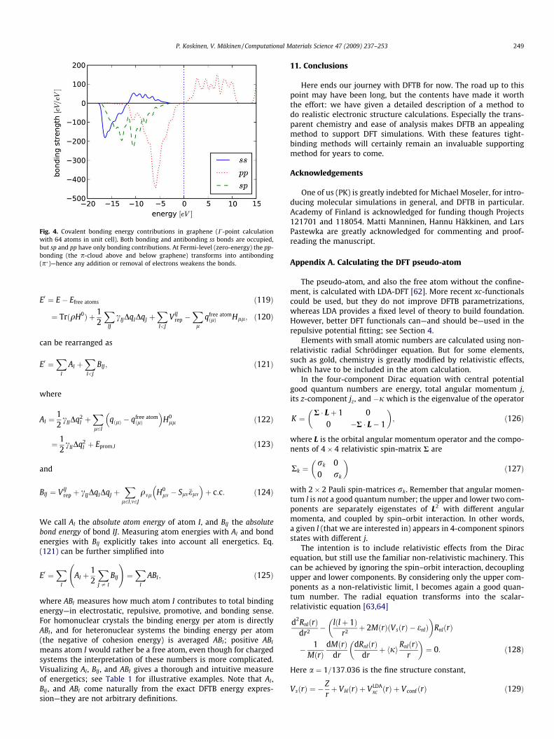
Fig. 4. Covalent bonding energy contributions in graphene (C-point calculationwith 64 atoms in unit cell). Both bonding and antibonding ss bonds are occupied,but sp and pp have only bonding contributions. At Fermi-level (zero-energy) the pp-bonding (the p-cloud above and below graphene) transforms into antibonding(p)—hence any addition or removal of electrons weakens the bonds.

P. Koskinen, V. Mäkinen / Computational Materials Science 47 (2009) 237–253 249

E0 ¼ E� Efree atoms ð119Þ

¼ TrðqH0Þ þ 12

XIJ

cIJDqIDqJ þXI<J

VIJrep �

Xl

qfree atomðlÞ Hll; ð120Þ

can be rearranged as

E0 ¼X

I

AI þXI<J

BIJ; ð121Þ

where

AI ¼12cIIDq2

I þXl2I

qðlÞ � qfree atomðlÞ

� �H0

ll ð122Þ

¼ 12cIIDq2

I þ Eprom;I ð123Þ

and

BIJ ¼ VIJrep þ cIJDqIDqJ þ

Xl2I;m2J

qml H0lm � Slm�elm

� �þ c:c: ð124Þ

We call AI the absolute atom energy of atom I, and BIJ the absolutebond energy of bond IJ. Measuring atom energies with AI and bondenergies with BIJ explicitly takes into account all energetics. Eq.(121) can be further simplified into

E0 ¼X

I

AI þ12

XJ – I

BIJ

!¼X

I

ABI; ð125Þ

where ABI measures how much atom I contributes to total bindingenergy—in electrostatic, repulsive, promotive, and bonding sense.For homonuclear crystals the binding energy per atom is directlyABI , and for heteronuclear systems the binding energy per atom(the negative of cohesion energy) is averaged ABI; positive ABI

means atom I would rather be a free atom, even though for chargedsystems the interpretation of these numbers is more complicated.Visualizing AI , BIJ , and ABI gives a thorough and intuitive measureof energetics; see Table 1 for illustrative examples. Note that AI ,BIJ , and ABI come naturally from the exact DFTB energy expres-sion—they are not arbitrary definitions.

11. Conclusions

Here ends our journey with DFTB for now. The road up to thispoint may have been long, but the contents have made it worththe effort: we have given a detailed description of a method todo realistic electronic structure calculations. Especially the trans-parent chemistry and ease of analysis makes DFTB an appealingmethod to support DFT simulations. With these features tight-binding methods will certainly remain an invaluable supportingmethod for years to come.

Acknowledgements

One of us (PK) is greatly indebted for Michael Moseler, for intro-ducing molecular simulations in general, and DFTB in particular.Academy of Finland is acknowledged for funding though Projects121701 and 118054. Matti Manninen, Hannu Häkkinen, and LarsPastewka are greatly acknowledged for commenting and proof-reading the manuscript.

Appendix A. Calculating the DFT pseudo-atom

The pseudo-atom, and also the free atom without the confine-ment, is calculated with LDA-DFT [62]. More recent xc-functionalscould be used, but they do not improve DFTB parametrizations,whereas LDA provides a fixed level of theory to build foundation.However, better DFT functionals can—and should be—used in therepulsive potential fitting; see Section 4.

Elements with small atomic numbers are calculated using non-relativistic radial Schrödinger equation. But for some elements,such as gold, chemistry is greatly modified by relativistic effects,which have to be included in the atom calculation.

In the four-component Dirac equation with central potentialgood quantum numbers are energy, total angular momentum j,its z-component jz, and �j which is the eigenvalue of the operator

K ¼R � Lþ 1 0

0 �R � L� 1

� �; ð126Þ

where L is the orbital angular momentum operator and the compo-nents of 4� 4 relativistic spin-matrix R are

Rk ¼rk 00 rk

� �ð127Þ

with 2� 2 Pauli spin-matrices rk. Remember that angular momen-tum l is not a good quantum number; the upper and lower two com-ponents are separately eigenstates of L2 with different angularmomenta, and coupled by spin–orbit interaction. In other words,a given l (that we are interested in) appears in 4-component spinorsstates with different j.

The intention is to include relativistic effects from the Diracequation, but still use the familiar non-relativistic machinery. Thiscan be achieved by ignoring the spin–orbit interaction, decouplingupper and lower components. By considering only the upper com-ponents as a non-relativistic limit, l becomes again a good quan-tum number. The radial equation transforms into the scalar-relativistic equation [63,64]

d2RnlðrÞdr2 � lðlþ 1Þ

r2 þ 2MðrÞðVsðrÞ � enlÞ� �

RnlðrÞ

� 1MðrÞ

dMðrÞdr

dRnlðrÞdr

þ hjiRnlðrÞr

� �¼ 0: ð128Þ

Here a ¼ 1=137:036 is the fine structure constant,

VsðrÞ ¼ �Zrþ VHðrÞ þ VLDA

xc ðrÞ þ V confðrÞ ð129Þ

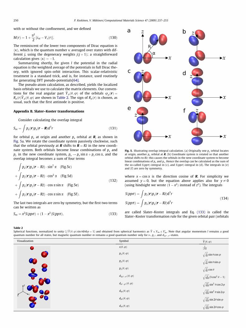
Fig. 5. Illustrating overlap integral calculation. (a) Originally one px orbital locatesat origin, another px orbital at R. (b) Coordinate system is rotated so that anotherorbital shifts to Rz; this causes the orbitals in the new coordinate system to becomelinear combinations of px and pz . Hence the overlap can be calculated as the sum ofthe so-called SðpppÞ-integral in (c), and SðpprÞ-integral in (d). The integrals in (e)and (f) are zero by symmetry.

250 P. Koskinen, V. Mäkinen / Computational Materials Science 47 (2009) 237–253

with or without the confinement, and we defined

MðrÞ ¼ 1þ a2

2½enl � VsðrÞ�: ð130Þ

The reminiscent of the lower two components of Dirac equation ishji, which is the quantum number j averaged over states with dif-ferent j, using the degeneracy weights jðjþ 1Þ; a straightforwardcalculation gives hji ¼ �1.

Summarizing shortly, for given l the potential in the radialequation is the weighted average of the potentials in full Dirac the-ory, with ignored spin–orbit interaction. This scalar-relativistictreatment is a standard trick, and is, for instance, used routinelyfor generating DFT pseudo-potentials[64].

The pseudo-atom calculation, as described, yields the localizedbasis orbitals we use to calculate the matrix elements. Our conven-tions for the real angular part eY lðh;uÞ of the orbitals ulðrÞ ¼RlðrÞeY lðh;uÞ are shown in Table 2. The sign of RlðrÞ is chosen, asusual, such that the first antinode is positive.

Appendix B. Slater–Koster transformations

Consider calculating the overlap integral

Sxx ¼Z

pxðrÞpxðr � RÞd3r ð131Þ

for orbital px at origin and another px orbital at R, as shown inFig. 5a. We rotate the coordinate system passively clockwise, suchthat the orbital previously at R shifts to R ¼ Rz in the new coordi-nate system. Both orbitals become linear combinations of px andpz in the new coordinate system, px ! px sinaþ pz cosa, and theoverlap integral becomes a sum of four termsZ

pxðrÞpxðr � RzÞ � sin2 a ðFig:5cÞ

þZ

pzðrÞpzðr � RzÞ � cos2 a ðFig:5dÞ

þZ

pxðrÞpzðr � RzÞ � cos a sina ðFig:5eÞ

þZ

pzðrÞpxðr � RzÞ � cos a sina ðFig:5fÞ:

ð132Þ

The last two integrals are zero by symmetry, but the first two termscan be written as

Sxx ¼ x2SðpprÞ þ ð1� x2ÞSðpppÞ; ð133Þ

Table 2Spherical functions, normalized to unity (

R eY ðh;uÞ sin hdhdu ¼ 1) and obtained from sphquantum number for all states, but magnetic quantum number m remains a good quantu

Visualization Sym

sðh;

pxðh

pyðh

pzðh

d3z2�

dx2�

dxyð

dyzð

dzxð

where x ¼ cos a is the direction cosine of R. For simplicity weassumed y ¼ 0, but the equation above applies also for y – 0(using hindsight we wrote ð1� x2Þ instead of z2). The integrals

SðpprÞ ¼Z

pzðrÞpzðr � RzÞd3r

SðpppÞ ¼Z

pxðrÞpxðr � RzÞd3rð134Þ

are called Slater–Koster integrals and Eq. (133) is called theSlater–Koster transformation rule for the given orbital pair (orbitals

erical harmonics as eY / Ylm Ylm . Note that angular momentum l remains a goodm number only for s-, pz-, and d3z2�r2 -states.

bol eY ðh;uÞuÞ 1ffiffiffiffiffi

4pp

;uÞ ffiffiffiffiffi3

4p

qsin h cos u

;uÞ ffiffiffiffiffi3

4p

qsin h sinu

;uÞ ffiffiffiffiffi3

4p

qcos h

r2 ðh;uÞffiffiffiffiffiffiffi

516p

qð3 cos2 h� 1Þ

y2 ðh;uÞffiffiffiffiffiffiffi15

16p

qsin2 h cos 2u

h;uÞ ffiffiffiffiffiffiffi15

16p

qsin2 h sin 2u

h;uÞ ffiffiffiffiffiffiffi15

16p

qsin 2h sin u

h;uÞ ffiffiffiffiffiffiffi15

16p

qsin 2h cos u

P. Koskinen, V. Mäkinen / Computational Materials Science 47 (2009) 237–253 251

may have different radial parts; the notation SlmðpprÞ stands for ra-dial functions RlðrÞ and RmðrÞ in the basis functions l and m). Similarreasoning can be applied for other combinations of p-orbitals aswell—they all reduce to Slater–Koster transformation rules involv-ing SðpprÞ and SðpppÞ integrals alone. This means that only twointegrals with a fixed R is needed for all overlaps between anytwo p-orbitals from a given element pair.

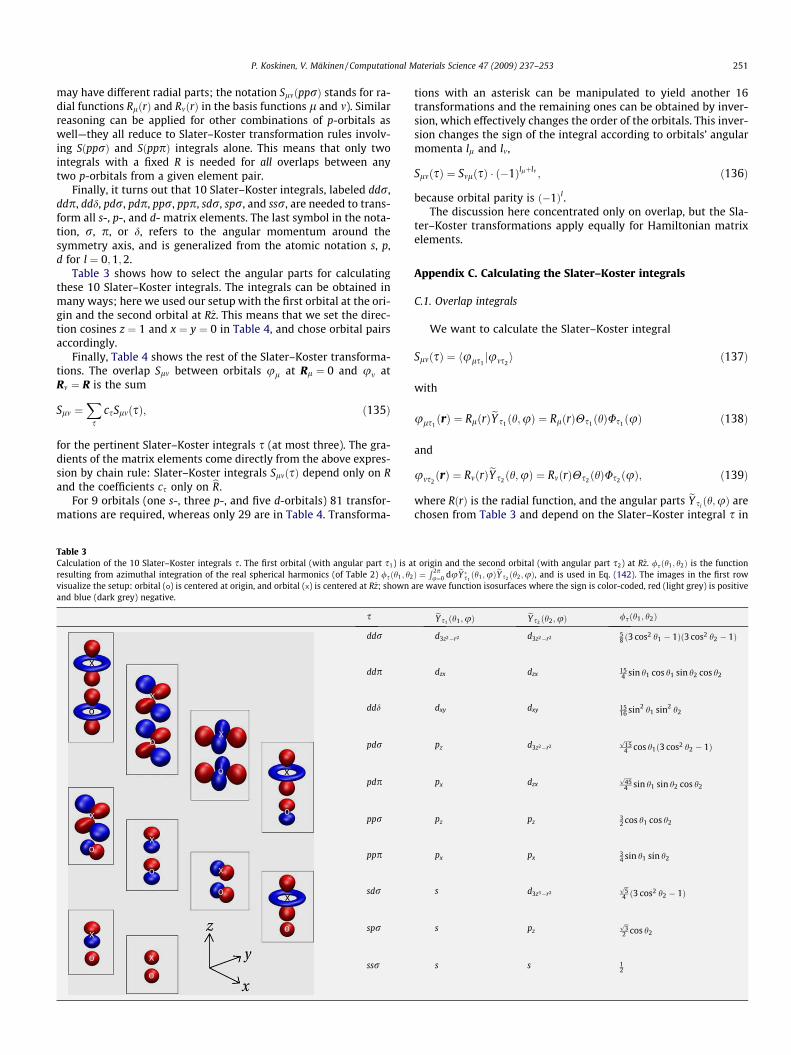
Finally, it turns out that 10 Slater–Koster integrals, labeled ddr,ddp, ddd, pdr, pdp, ppr, ppp, sdr, spr, and ssr, are needed to trans-form all s-, p-, and d- matrix elements. The last symbol in the nota-tion, r, p, or d, refers to the angular momentum around thesymmetry axis, and is generalized from the atomic notation s, p,d for l ¼ 0;1;2.

Table 3 shows how to select the angular parts for calculatingthese 10 Slater–Koster integrals. The integrals can be obtained inmany ways; here we used our setup with the first orbital at the ori-gin and the second orbital at Rz. This means that we set the direc-tion cosines z ¼ 1 and x ¼ y ¼ 0 in Table 4, and chose orbital pairsaccordingly.

Finally, Table 4 shows the rest of the Slater–Koster transforma-tions. The overlap Slm between orbitals ul at Rl ¼ 0 and um atRm ¼ R is the sum

Slm ¼X

scsSlmðsÞ; ð135Þ

for the pertinent Slater–Koster integrals s (at most three). The gra-dients of the matrix elements come directly from the above expres-sion by chain rule: Slater–Koster integrals SlmðsÞ depend only on Rand the coefficients cs only on bR.

For 9 orbitals (one s-, three p-, and five d-orbitals) 81 transfor-mations are required, whereas only 29 are in Table 4. Transforma-

Table 3Calculation of the 10 Slater–Koster integrals s. The first orbital (with angular part s1) is aresulting from azimuthal integration of the real spherical harmonics (of Table 2) /sðh1 ; h2

visualize the setup: orbital (o) is centered at origin, and orbital (x) is centered at Rz; shownand blue (dark grey) negative.

s

ddr

ddp

ddd

pdr

pdp

ppr

ppp

sdr

spr

ssr

tions with an asterisk can be manipulated to yield another 16transformations and the remaining ones can be obtained by inver-sion, which effectively changes the order of the orbitals. This inver-sion changes the sign of the integral according to orbitals’ angularmomenta ll and lm,

SlmðsÞ ¼ SmlðsÞ � ð�1Þllþlm ; ð136Þ

because orbital parity is ð�1Þl.The discussion here concentrated only on overlap, but the Sla-

ter–Koster transformations apply equally for Hamiltonian matrixelements.

Appendix C. Calculating the Slater–Koster integrals

C.1. Overlap integrals

We want to calculate the Slater–Koster integral

SlmðsÞ ¼ huls1jums2

i ð137Þ

with

uls1ðrÞ ¼ RlðrÞeY s1 ðh;uÞ ¼ RlðrÞHs1 ðhÞUs1 ðuÞ ð138Þ

and

ums2ðrÞ ¼ RmðrÞeY s2 ðh;uÞ ¼ RmðrÞHs2 ðhÞUs2 ðuÞ; ð139Þ

where RðrÞ is the radial function, and the angular parts eY siðh;uÞ are

chosen from Table 3 and depend on the Slater–Koster integral s in

t origin and the second orbital (with angular part s2) at Rz. /sðh1 ; h2Þ is the functionÞ ¼

R 2pu¼0 dueY s1

ðh1;uÞeY s2 ðh2;uÞ, and is used in Eq. (142). The images in the first roware wave function isosurfaces where the sign is color-coded, red (light grey) is positive

eY s1 ðh1;uÞ eY s2 ðh2;uÞ /sðh1; h2Þ

d3z2�r2 d3z2�r2 58 ð3 cos2 h1 � 1Þð3 cos2 h2 � 1Þ

dzx dzx 154 sin h1 cos h1 sin h2 cos h2

dxy dxy 1516 sin2 h1 sin2 h2

pz d3z2�r2ffiffiffiffi15p

4 cos h1ð3 cos2 h2 � 1Þ

px dzxffiffiffiffi45p

4 sin h1 sin h2 cos h2

pz pz32 cos h1 cos h2

px px34 sin h1 sin h2

s d3z3�r2ffiffi5p

4 ð3 cos2 h2 � 1Þ

s pzffiffi3p

2 cos h2

s s 12

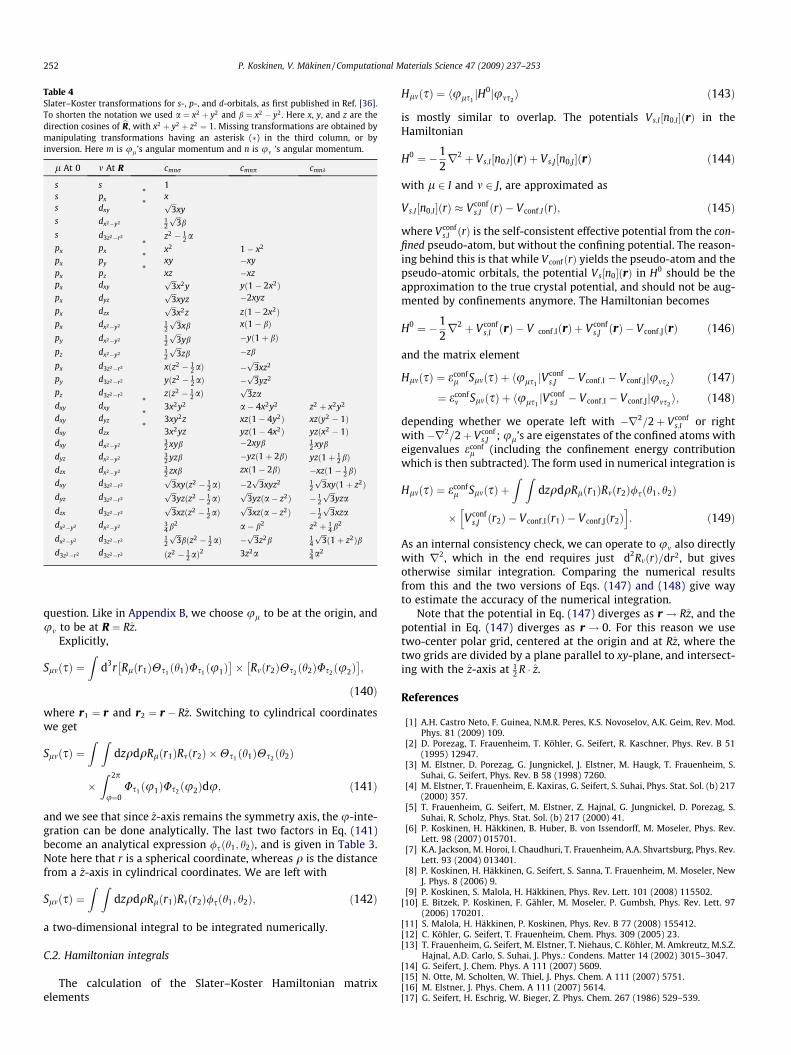
Table 4Slater–Koster transformations for s-, p-, and d-orbitals, as first published in Ref. [36].To shorten the notation we used a ¼ x2 þ y2 and b ¼ x2 � y2. Here x, y, and z are thedirection cosines of bR, with x2 þ y2 þ z2 ¼ 1. Missing transformations are obtained bymanipulating transformations having an asterisk () in the third column, or byinversion. Here m is ul ’s angular momentum and n is um ’s angular momentum.

l At 0 m At R cmnr cmnp cmnd

s s 1s px

* xs dxy

* ffiffiffi3p

xys dx2�y2 1

2

ffiffiffi3p

b

s d3z2�r2 z2 � 12 a

px px* x2 1� x2

px py* xy �xy

px pz* xz �xz

px dxyffiffiffi3p

x2y yð1� 2x2Þpx dyz

ffiffiffi3p

xyz �2xyz

px dzxffiffiffi3p

x2z zð1� 2x2Þpx dx2�y2 1

2

ffiffiffi3p

xb xð1� bÞpy dx2�y2 1

2

ffiffiffi3p

yb �yð1þ bÞpz dx2�y2 1

2

ffiffiffi3p

zb �zb

px d3z2�r2 xðz2 � 12 aÞ �

ffiffiffi3p

xz2

py d3z2�r2 yðz2 � 12 aÞ �

ffiffiffi3p

yz2

pz d3z2�r2 zðz2 � 12 aÞ

ffiffiffi3p

zadxy dxy

* 3x2y2 a� 4x2y2 z2 þ x2y2

dxy dyz* 3xy2z xzð1� 4y2Þ xzðy2 � 1Þ

dxy dzx* 3x2yz yzð1� 4x2Þ yzðx2 � 1Þ

dxy dx2�y2 32 xyb �2xyb 1

2 xyb

dyz dx2�y2 32 yzb �yzð1þ 2bÞ yzð1þ 1

2 bÞdzx dx2�y2 3

2 zxb zxð1� 2bÞ �xzð1� 12 bÞ

dxy d3z2�r2ffiffiffi3p

xyðz2 � 12 aÞ �2

ffiffiffi3p

xyz2 12

ffiffiffi3p

xyð1þ z2Þdyz d3z2�r2

ffiffiffi3p

yzðz2 � 12 aÞ

ffiffiffi3p

yzða� z2Þ � 12

ffiffiffi3p

yzadzx d3z2�r2

ffiffiffi3p

xzðz2 � 12 aÞ

ffiffiffi3p

xzða� z2Þ � 12

ffiffiffi3p

xzadx2�y2 dx2�y2 3

4 b2 a� b2 z2 þ 14 b2

dx2�y2 d3z2�r2 12

ffiffiffi3p

bðz2 � 12 aÞ �

ffiffiffi3p

z2b 14

ffiffiffi3pð1þ z2Þb

d3z2�r2 d3z2�r2 ðz2 � 12 aÞ2 3z2a 3

4 a2

252 P. Koskinen, V. Mäkinen / Computational Materials Science 47 (2009) 237–253

question. Like in Appendix B, we choose ul to be at the origin, andum to be at R ¼ Rz.

Explicitly,

SlmðsÞ ¼Z

d3r Rlðr1ÞHs1 ðh1ÞUs1 ðu1Þ �

� Rmðr2ÞHs2 ðh2ÞUs2 ðu2Þ �

;

ð140Þ

where r1 ¼ r and r2 ¼ r � Rz. Switching to cylindrical coordinateswe get

SlmðsÞ ¼Z Z

dzqdqRlðr1ÞRmðr2Þ �Hs1 ðh1ÞHs2 ðh2Þ

�Z 2p

u¼0Us1 ðu1ÞUs2 ðu2Þdu; ð141Þ

and we see that since z-axis remains the symmetry axis, the u-inte-gration can be done analytically. The last two factors in Eq. (141)become an analytical expression /sðh1; h2Þ, and is given in Table 3.Note here that r is a spherical coordinate, whereas q is the distancefrom a z-axis in cylindrical coordinates. We are left with

SlmðsÞ ¼Z Z

dzqdqRlðr1ÞRmðr2Þ/sðh1; h2Þ; ð142Þ

a two-dimensional integral to be integrated numerically.

C.2. Hamiltonian integrals

The calculation of the Slater–Koster Hamiltonian matrixelements

HlmðsÞ ¼ huls1jH0jums2

i ð143Þ

is mostly similar to overlap. The potentials Vs;I½n0;I�ðrÞ in theHamiltonian

H0 ¼ �12r2 þ Vs;I½n0;I�ðrÞ þ Vs;J ½n0;J �ðrÞ ð144Þ

with l 2 I and m 2 J, are approximated as

Vs;I½n0;I�ðrÞ � Vconfs;I ðrÞ � Vconf;IðrÞ; ð145Þ

where V confs;I ðrÞ is the self-consistent effective potential from the con-

fined pseudo-atom, but without the confining potential. The reason-ing behind this is that while VconfðrÞ yields the pseudo-atom and thepseudo-atomic orbitals, the potential Vs½n0�ðrÞ in H0 should be theapproximation to the true crystal potential, and should not be aug-mented by confinements anymore. The Hamiltonian becomes

H0 ¼ �12r2 þ Vconf

s;I ðrÞ � V conf;IðrÞ þ V confs;J ðrÞ � V conf;JðrÞ ð146Þ

and the matrix element

HlmðsÞ ¼ econfl SlmðsÞ þ huls1

jVconfs;J � Vconf;I � Vconf;Jjums2

i ð147Þ

¼ econfm SlmðsÞ þ huls1

jVconfs;I � Vconf;I � V conf;Jjums2

i; ð148Þ

depending whether we operate left with �r2=2þ Vconfs;I or right

with �r2=2þ Vconfs;J ; ul’s are eigenstates of the confined atoms with

eigenvalues econfl (including the confinement energy contribution

which is then subtracted). The form used in numerical integration is

HlmðsÞ ¼ econfl SlmðsÞ þ

Z ZdzqdqRlðr1ÞRmðr2Þ/sðh1; h2Þ

� V confs;J ðr2Þ � Vconf;Iðr1Þ � V conf;Jðr2Þ

h i: ð149Þ

As an internal consistency check, we can operate to um also directlywith r2, which in the end requires just d2RmðrÞ=dr2, but givesotherwise similar integration. Comparing the numerical resultsfrom this and the two versions of Eqs. (147) and (148) give wayto estimate the accuracy of the numerical integration.

Note that the potential in Eq. (147) diverges as r ! Rz, and thepotential in Eq. (147) diverges as r ! 0. For this reason we usetwo-center polar grid, centered at the origin and at Rz, where thetwo grids are divided by a plane parallel to xy-plane, and intersect-ing with the z-axis at 1

2 R � z.

References

[1] A.H. Castro Neto, F. Guinea, N.M.R. Peres, K.S. Novoselov, A.K. Geim, Rev. Mod.Phys. 81 (2009) 109.

[2] D. Porezag, T. Frauenheim, T. Köhler, G. Seifert, R. Kaschner, Phys. Rev. B 51(1995) 12947.

[3] M. Elstner, D. Porezag, G. Jungnickel, J. Elstner, M. Haugk, T. Frauenheim, S.Suhai, G. Seifert, Phys. Rev. B 58 (1998) 7260.

[4] M. Elstner, T. Frauenheim, E. Kaxiras, G. Seifert, S. Suhai, Phys. Stat. Sol. (b) 217(2000) 357.

[5] T. Frauenheim, G. Seifert, M. Elstner, Z. Hajnal, G. Jungnickel, D. Porezag, S.Suhai, R. Scholz, Phys. Stat. Sol. (b) 217 (2000) 41.

[6] P. Koskinen, H. Häkkinen, B. Huber, B. von Issendorff, M. Moseler, Phys. Rev.Lett. 98 (2007) 015701.

[7] K.A. Jackson, M. Horoi, I. Chaudhuri, T. Frauenheim, A.A. Shvartsburg, Phys. Rev.Lett. 93 (2004) 013401.

[8] P. Koskinen, H. Häkkinen, G. Seifert, S. Sanna, T. Frauenheim, M. Moseler, NewJ. Phys. 8 (2006) 9.

[9] P. Koskinen, S. Malola, H. Häkkinen, Phys. Rev. Lett. 101 (2008) 115502.[10] E. Bitzek, P. Koskinen, F. Gähler, M. Moseler, P. Gumbsh, Phys. Rev. Lett. 97

(2006) 170201.[11] S. Malola, H. Häkkinen, P. Koskinen, Phys. Rev. B 77 (2008) 155412.[12] C. Köhler, G. Seifert, T. Frauenheim, Chem. Phys. 309 (2005) 23.[13] T. Frauenheim, G. Seifert, M. Elstner, T. Niehaus, C. Köhler, M. Amkreutz, M.S.Z.

Hajnal, A.D. Carlo, S. Suhai, J. Phys.: Condens. Matter 14 (2002) 3015–3047.[14] G. Seifert, J. Chem. Phys. A 111 (2007) 5609.[15] N. Otte, M. Scholten, W. Thiel, J. Phys. Chem. A 111 (2007) 5751.[16] M. Elstner, J. Phys. Chem. A 111 (2007) 5614.[17] G. Seifert, H. Eschrig, W. Bieger, Z. Phys. Chem. 267 (1986) 529–539.

P. Koskinen, V. Mäkinen / Computational Materials Science 47 (2009) 237–253 253

[18] W.M.C. Foulkes, R. Haydock, Phys. Rev. B 39 (1989) 12520.[19] O.F. Sankey, D.J. Niklewski, Phys. Rev. B 40 (1989) 3979.[20] T. Frauenheim, F. Weich, T. Köhler, S. Uhlmann, D. Porezag, G. Seifert, Phys.

Rev. B 52 (1995) 11492.[21] G. Seifert, D. Porezag, T. Frauenheim, Int. J. Quant. Chem. 58 (1996) 185–192.[22] J. Widany, T. Frauenheim, T. Köhler, M. Sternberg, D. Porezag, G. Jungnickel, G.

Seifert, Phys. Rev. B 53 (1996) 4443.[23] F. Liu, Phys. Rev. B 52 (1995) 10677.[24] T.N. Todorov, J. Phys.: Condens. Matter 13 (2001) 10125–10148.[25] B. Torralva, T.A. Niehaus, M. Elstner, S. Suhai, T. Frauenheim, R.E. Allen, Phys.

Rev. B 64 (2001) 153105.[26] T.A. Niehaus, D. Heringer, B. Torralva, T. Frauenheim, Eur. Phys. J. D 35 (2005)

467–477.[27] J.R. Reimers, G.C. Solomon, A. Gagliardi, A. Bilic, N.S. Hush, T. Frauenheim, A.D.

Carlo, A. Pecchia, J. Phys. Chem. A 111 (2007) 5692.[28] T.A. Niehaus, S. Suhai, F.D. Sala, P. Lugli, M. Elstner, G. Seifert, T. Frauenheim,

Phys. Rev. B 63 (2001) 085108.[29] Hotbit wiki at <https://trac.cc.jyu.fi/projects/hotbit>.[30] <http://www.gnu.org/licenses/gpl.html>.[31] ASE wiki at <https://wiki.fysik.dtu.dk/ase/>.[32] R.G. Parr, W. Yang, Density-Functional Theory of Atoms and Molecules, Oxford

University Press, 1994.[33] N. Bernstein, M.J. Mehl, D.A. Papaconstantopoulos, Phys. Rev. B 66 (2002)

075212.[34] R.S. Mulliken, J. Chem. Phys. 23 (1955) 1833.[35] J. Junquera, O. Paz, D. Sanchez-Portal, E. Artacho, Phys. Rev. B 64 (2001)

235111.[36] J.C. Slater, G.F. Koster, Phys. Rev. 94 (1954) 1498.[37] J.A. Pople, J. Chem. Phys. 37 (1962) 53.[38] T.B. Boykin, R.C. Bowen, G. Klimeck, Phys. Rev. B 63 (2001) 245314.[39] M. Graf, P. Vogl, Phys. Rev. B 51 (1995) 4940.[40] I.N. Bronshtein, K.A. Semendyayev, G. Musiol, H. Muehlig, Handbook of

Mathematics, Springer, 2004.[41] <http://www.dftb.org>.

[42] J.J. Mortensen, L.B. Hansen, K.W. Jacobsen, Phys. Rev. B 71 (2005) 035109.[43] GPAW wiki at <https://wiki.fysik.dtu.dk/gpaw>.[44] J.P. Perdew, K. Burke, M. Ernzerhof, Phys. Rev. Lett. 77 (1996) 3865.[45] H. Rydberg, M. Dion, N. Jacobson, E. Scroder, P. Hyldgaard, S.I. Simak, D.C.

Langreth, B.I. Lundqvist, Phys. Rev. Lett. 91 (2003) 126402.[46] T.A. Halgren, J. Am. Chem. Soc. 114 (1992) 7827.[47] M. Elstner, P. Hobza, T. Frauenheim, S. Suhai, E. Kaxiras, J. Chem. Phys. 114

(2001) 5149.[48] P. Koskinen, L. Sapienza, M. Manninen, Phys. Scripta 68 (2003) 74–78.[49] N.W. Ashcroft, N.D. Mermin, Solid State Physics, Saunders College Publishing,

1976.[50] H.J. Monkhorst, J.D. Pack, Phys. Rev. B 13 (1976) 5188.[51] D. Frenkel, B. Smit, Understanding molecular simulation, From Algorithms to

Applications, Academic Press, 2002.[52] S. Malola, H. Häkkinen, P. Koskinen, Phys. Rev. B 78 (2008) 153409.[53] C.P. Liu, J.W. Ding, J. Phys.:Condens. Matter 18 (2006) 4077.[54] V.N. Popov, New J. Phys. 6 (2004) 17.[55] P.W. Atkins, R.S. Friedman, Molecular Quantum Mechanics, Oxford University

Press, 2000.[56] O. Kit, P. Koskinen, in preparation.[57] I. Mayer, Simple Theorems, Proofs, and Derivations in Quantum Chemistry,

Springer, 2003.[58] B. Yoon, P. Koskinen, B. Huber, O. Kostko, B. von Issendorff, H. Häkkinen, M.

Moseler, U. Landman, Chem. Phys. Chem. 8 (2006) 157–161.[59] F. Yin, J. Akola, P. Koskinen, M. Manninen, R.E. Palmer, Phys. Rev. Lett. 102

(2009) 106102.[60] A.J. Bridgeman, G. Cavigliasso, L.R. Ireland, J. Rothery, J. Chem. Soc., Dalton

Trans. 2001 (2001) 2095–2108.[61] N. Börnsen, B. Meyer, O. Grotheer, M. Fähnle, J. Phys.: Condens. Matter 11

(1999) L287.[62] J.P. Perdew, Y. Wang, Phys. Rev. B 45 (1992) 13244.[63] D.D. Koelling, B.N. Harmon, J. Phys. C 10 (1977) 3107.[64] R.M. Martin, Electronic Structure Basic Theory and Practical Methods,

Cambridge University Press, 2004.