calder on problem - jyväskylän...
TRANSCRIPT
Calderon problem
Lecture notes, Spring 2008
Mikko Salo
Department of Mathematics and Statistics
University of Helsinki

Contents
Chapter 1. Introduction 1
Chapter 2. Multiple Fourier series 5
2.1. Fourier series in L2 5
2.2. Sobolev spaces 11
Chapter 3. Uniqueness 15
3.1. Reduction to Schrodinger equation 15
3.2. Complex geometrical optics 20
3.3. Uniqueness proof 26
Chapter 4. Stability 29
4.1. Schrodinger equation 31
4.2. More facts on Sobolev spaces 33
4.3. Conductivity equation 37
Chapter 5. Partial data 41
5.1. Carleman estimates 41
5.2. Uniqueness with partial data 50
Bibliography 55
v

CHAPTER 1
Introduction
Electrical Impedance Tomography (EIT) is an imaging method with
potential applications in medical imaging and nondestructive testing.
The method is based on the following important inverse problem.
Calderon problem: Is it possible to determine the
electrical conductivity of a medium by making voltage
and current measurements on its boundary?
In this course we will prove a fundamental uniqueness result due
to Sylvester and Uhlmann, which states that the conductivity is de-
termined by the boundary measurements. We will also consider stable
dependence of the conductivity on boundary measurements, and the
case where measurements are only made on part of the boundary. In
addition, we will discuss useful techniques in partial differential equa-
tions, Fourier analysis, and inverse problems.
Let us begin by recalling the mathematical model of EIT, see [5] for
details. The purpose is to determine the electrical conductivity γ(x) at
each point x ∈ Ω, where Ω ⊆ Rn represents the body which is imaged
(in practice n = 3). We assume that Ω is a bounded open subset of Rn
with C∞ boundary, and that γ is a positive C2 function in Ω.
Under the assumption of no sources or sinks of current in Ω, a
voltage potential f at the boundary ∂Ω induces a voltage potential u
in Ω, which solves the Dirichlet problem for the conductivity equation,
(1.1)
∇ · γ∇u = 0 in Ω,
u = f on ∂Ω.
Since γ is positive, there is a unique weak solution u ∈ H1(Ω) for
any boundary value f ∈ H1/2(∂Ω). One can define the Dirichlet to
Neumann map (DN map) formally as
Λγf = γ∂u
∂ν
∣∣∣∂Ω.
1
2 1. INTRODUCTION
This is the current flowing through the boundary. More precisely, the
DN map is defined weakly as
(Λγf, g)∂Ω =
∫Ω
γ∇u · ∇v dx, f, g ∈ H1/2(∂Ω),
where u is the solution of (1.1), and v is any function in H1(Ω) with
v|∂Ω = g. The pairing on the boundary is integration with respect to
the surface measure,
(f, g)∂Ω =
∫∂Ω
fg dS.
With this definition Λγ is a bounded linear map from H1/2(∂Ω) into
H−1/2(∂Ω).
The Calderon problem (also called the inverse conductivity prob-
lem) is to determine the conductivity function γ from the knowledge
of the map Λγ. That is, if the measured current Λγf is known for all
boundary voltages f ∈ H1/2(∂Ω), one would like to determine the con-
ductivity γ. There are several aspects of this inverse problem which are
interesting both for mathematical theory and practical applications.
1. Uniqueness. If Λγ1 = Λγ2 , show that γ1 = γ2.
2. Reconstruction. Given the boundary measurements Λγ, find
a procedure to reconstruct the conductivity γ.
3. Stability. If Λγ1 is close to Λγ2 , show that γ1 and γ2 are close
(in a suitable sense).
4. Partial data. If Γ is a subset of ∂Ω and if Λγ1f |Γ = Λγ2f |Γfor all boundary voltages f , show that γ1 = γ2.
Starting from the work of Calderon in 1980, the inverse conductivity
problem has been studied intensively. In the case where n ≥ 3 and
all conductivities are in C2(Ω), the following positive results are an
example of what can be proved.
Theorem. (Sylvester-Uhlmann 1987) If Λγ1 = Λγ2, then γ1 = γ2
in Ω.
Theorem. (Nachman 1988) There is a convergent algorithm for
reconstructing γ from Λγ.
Theorem. (Alessandrini 1988) Let γj ∈ Hs(Ω) for s > n2
+ 2, and
assume that ‖γj‖Hs(Ω) ≤M and 1/M ≤ γj ≤M (j = 1, 2). Then
‖γ1 − γ2‖L∞(Ω) ≤ ω(‖Λγ1 − Λγ2‖H1/2(∂Ω)→H−1/2(∂Ω))
1. INTRODUCTION 3
where ω(t) = C|log t|−σ for small t > 0, with C = C(Ω,M, n, s) > 0,
σ = σ(n, s) ∈ (0, 1).
Theorem. (Kenig-Sjostrand-Uhlmann 2007) Assume that Ω is con-
vex and Γ is any open subset of ∂Ω. If Λγ1f |Γ = Λγ2f |Γ for all
f ∈ H1/2(∂Ω), and if γ1|∂Ω = γ2|∂Ω, then γ1 = γ2 in Ω.
During this course we will discuss the methods involved in these re-
sults. The main tool will be the construction of special solutions, called
complex geometrical optics solutions, to the conductivity equation and
related equations. This will involve Fourier analysis, and we will begin
the course with a discussion of n-dimensional Fourier series.
References. This course a continuation of the class ”Impedanssi-
tomografian perusteet” (Principles of EIT) given by Petri Ola [5]. From
[5] we will mainly use the solvability of the Dirichlet problem for el-
liptic equations, the definition of the DN map, and results which state
that the boundary values of the conductivity can be recovered from the
DN map. Chapter 2 on multiple Fourier series is classical, an excellent
reference is Zygmund [8]. In Chapter 3 we prove the uniqueness result
of Sylvester-Uhlmann [6]. The proof of the main estimate, Theorem
3.7, follows Hahner [4]. The stability question is taken up in Chapter 4,
where the main results are due to Alessandrini [1]. The treatment also
benefited from Feldman-Uhlmann [3]. In the final Chapter 5 we intro-
duce Carleman estimates and prove the result in Bukhgeim-Uhlmann
[2], which states that it is enough to measure currents on roughly half
of the boundary to determine the conductivity.

CHAPTER 2
Multiple Fourier series
2.1. Fourier series in L2
Joseph Fourier laid the foundations of the mathematical field now
known as Fourier analysis in his 1822 treatise on heat flow. The basic
question is to represent periodic functions as sums of elementary pieces.
If the period of f is 2π and the elementary pieces are sine and cosine
functions, then the desired representation would be
f(x) =∞∑k=0
(ak cos(kx) + bk sin(kx)).
Since eikx = cos(kx)+i sin(kx), we may alternatively consider the series
(2.1) f(x) =∞∑
k=−∞
ckeikx.
We will need to represent functions of n variables as Fourier series. If f
is a function in Rn which is 2π-periodic in each variable, then a natural
analog of (2.1) would be
f(x) =∑k∈Zn
ckeik·x.
This is the form of Fourier series which we will study. Note that the
terms on the right-hand side are 2π-periodic in each variable.
There are many subtle issues related to various modes of conver-
gence for the series above. However, we will mostly just need the case
of convergence in L2 norm for Fourier series of L2 functions, and in this
case no problems arise. Consider the cube Q = [−π, π]n, and define an
inner product on L2(Q) by
(f, g) = (2π)−n∫Q
fg dx, f, g ∈ L2(Q).
With this inner product, L2(Q) is a separable infinite-dimensional Hilbert
space. The space of functions which are locally square integrable and
5
6 2. MULTIPLE FOURIER SERIES
2π-periodic in each variable may be identified with L2(Q). Therefore,
we will consider Fourier series of functions in L2(Q).
Lemma 2.1. The set eik·x is an orthonormal subset of L2(Q).
Proof. A direct computation: if k, l ∈ Zn then
(eik·x, eil·x) = (2π)−n∫Q
ei(k−l)·x dx
= (2π)−n∫ π
−π· · ·∫ π
−πei(k1−l1)x1 · · · ei(kn−ln)xn dxn · · · dx1
=
1, k = l,
0, k 6= l.
We recall a Hilbert space fact: if ej∞j=1 is an orthonormal subset
of a separable Hilbert space H, then the following are equivalent:
(1) ej∞j=1 is an orthonormal basis, in the sense that any f ∈ Hmay be written as the series
f =∞∑j=1
(f, ej)ej
with convergence in H,
(2) for any f ∈ H one has
‖f‖2 =∞∑j=1
|(f, ej)|2,
(3) if f ∈ H and (f, ej) = 0 for all j, then f ≡ 0.
If the condition (3) is satisfied, the orthonormal system ej is called
complete. The main point is that eik·xk∈Zn is complete in L2(Q).
Lemma 2.2. If f ∈ L2(Q) satisfies (f, eik·x) = 0 for all k ∈ Zn,
then f ≡ 0.
The proof is given below. The main result on Fourier series of L2
functions is now immediate. Below we denote by `2(Zn) the space of
complex sequences c = (ck)k∈Zn with norm
‖c‖`2(Zn) =( ∑k∈Zn|ck|2
)1/2
.
2.1. FOURIER SERIES IN L2 7
Theorem 2.3. If f ∈ L2(Q), then one has the Fourier series
f(x) =∑k∈Zn
f(k)eik·x
with convergence in L2(Q), where the Fourier coefficients are given by
f(k) = (f, eik·x) = (2π)−n∫Q
f(x)e−ik·x dx.
One has the Plancherel formula
‖f‖2L2(Q) =
∑k∈Zn|f(k)|2.
Conversely, if c = (ck) ∈ `2(Zn), then the series
f(x) =∑k∈Zn
ckeik·x
converges in L2(Q) to a function f satisfying f(k) = ck.
Proof. The facts on the Fourier series of f ∈ L2(Q) follow directly
from the discussion above, since eik·xk∈Zn is a complete orthonormal
system in L2(Q). For the converse, if (ck) ∈ `2(Zn), then
‖∑k∈Zn
M≤|k|≤N
ckeik·x‖2
L2(Q) =∑k∈Zn
M≤|k|≤N
|ck|2
by orthogonality. Since the right hand side can be made arbitrarily
small by choosing M and N large, we see that fN =∑
k∈Zn,|k|≤N ckeik·x
is a Cauchy sequence in L2(Q), and converges to f ∈ L2(Q). One
obtains f(k) = (f, eik·x) = ck again by orthogonality.
It remains to prove Lemma 2.2. We begin with the most familiar
case, n = 1. The partial sums of the Fourier series of a function
f ∈ L2([−π, π]), extended as a 2π-periodic function into R, are given
by
Smf(x) =m∑
k=−m
f(k)eikx =m∑
k=−m
( 1
2π
∫ π
−πf(y)e−iky dy
)eikx
=
∫ π
−πDm(x− y)f(y) dy
8 2. MULTIPLE FOURIER SERIES
where Dm(x) is the Dirichlet kernel
Dm(x) =1
2π
m∑k=−m
eikx =1
2πe−imx(1 + eix + . . .+ ei2mx)
=1
2πe−imx
ei(2m+1)x − 1
eix − 1=
1
2π
ei(m+ 12
)x − e−i(m+ 12
)x
ei12x − e−i 1
2x
=1
2π
sin((m+ 12)x)
sin(12x)
.
Thus, definining the convolution of two 2π-periodic locally integrable
functions by
f ∗ g(x) =
∫ π
−πf(x− y)g(y) dy,
we see that Smf(x) = (Dm ∗ f)(x). The Dirichlet kernel acts in a
similar way as an approximate identity, but is problematic because it
takes both positive and negative values.
Definition. A sequence (KN(x))∞N=1 of 2π-periodic continuous
functions on the real line is called an approximate identity if
(1) KN ≥ 0 for all N ,
(2)∫ π−πKN(x) dx = 1 for all N , and
(3) for all δ > 0 one has
limN→∞
supδ≤|x|≤π
KN(x)→ 0.
Thus, an approximate identity (KN) for large N resembles a Dirac
delta at 0, extended in a 2π-periodic way. It is possible to approximate
Lp functions by convolving them against an approximate identity.
Lemma 2.4. Let (KN) be an approximate identity. If f ∈ Lp([−π, π])
where 1 ≤ p < ∞, or if f is a continuous 2π-periodic function and
p =∞, then
‖KN ∗ f − f‖Lp([−π,π]) → 0 as N →∞.
Proof. Since KN has integral 1, we have
(KN ∗ f)(x)− f(x) =
∫ π
−πKN(y)[f(x− y)− f(x)] dy
2.1. FOURIER SERIES IN L2 9
Let first f be continuous and p = ∞. To estimate the L∞ norm of
KN ∗ f − f , we fix ε > 0 and compute
|(KN ∗ f)(x)− f(x)| ≤∫ π
−πKN(y)|f(x− y)− f(x)| dy
≤∫|y|≤δ
KN(y)|f(x−y)−f(x)| dy+
∫δ≤|y|≤π
KN(y)|f(x−y)−f(x)| dy.
Here δ > 0 is chosen so that
|f(x− y)− f(x)| < ε
2whenever x ∈ R and |y| ≤ δ.
This is possible because f is uniformly continuous. Further, we use the
definition of an approximate identity and choose N0 so that
supδ≤|x|≤π
KN(x) <ε
4π‖f‖L∞, for N ≥ N0.
With these choices, we obtain
|(KN ∗ f)(x)− f(x)| ≤ ε
2
∫|y|≤δ
KN(y) dy + 4π‖f‖L∞ supδ≤|x|≤π
KN(x) < ε
whenever N ≥ N0. The result is proved in the case p =∞.
Let now f ∈ Lp([−π, π]) and 1 ≤ p < ∞. We need the integral
form of Minkowski’s inequality,(∫X
∣∣∣ ∫Y
F (x, y) dν(y)∣∣∣p dµ(x)
)1/p
≤∫Y
(∫X
|F (x, y)|p dµ(x))1/p
dν(y),
which is valid on σ-finite measure spaces (X,µ) and (Y, ν), cf. the
usual Minkowski inequality ‖∑
y F ( · , y)‖Lp ≤∑
y‖F ( · , y)‖Lp . Using
this, we obtain
‖KN ∗ f − f‖Lp([−π,π]) ≤∫ π
−πKN(y)‖f( · − y)− f‖Lp([−π,π]) dy
=
∫δ≤|y|≤π
KN(y)‖f( · −y)−f‖Lp dy+
∫|y|≤δ
KN(y)‖f( · −y)−f‖Lp dy
≤ 4π‖f‖Lp supδ≤|x|≤π
KN(x) + sup|y|≤δ‖f( · − y)− f‖Lp .
Now, for any ε > 0, there is δ > 0 such that
‖f( · − y)− f‖Lp([−π,π]) <ε
2whenever |y| ≤ δ.
Thus the second term can be made arbitrarily small by choosing δ
sufficiently small, and then the first term is also small if N is large.
This shows the result.

10 2. MULTIPLE FOURIER SERIES
Now, if the Dirichlet kernels (Dm) were an approximate identity, by
Lemma 2.4 one would have Smf → f in L2 for any f ∈ L2. This would
in particular imply that any f ∈ L2 which satisfies (f, eikx) = f(k) = 0
for all k ∈ Zn, would be the zero function.
However, Dm is not an approximate identity because it takes nega-
tive values. One does get an approximate identity if a different summa-
tion method used: instead of the partial sums Smf consider the Cesaro
sums
σNf(x) =1
N + 1
N∑m=0
Smf(x).
This can be written in convolution form as
σNf(x) =1
N + 1
N∑m=0
(Dm ∗ f)(x) = (FN ∗ f)(x)
where FN is the Fejer kernel,
FN(x) =1
2π(N + 1)
N∑m=0
ei(m+ 12
)x − e−i(m+ 12
)x
ei12x − e−i 1
2x
=1
2π(N + 1)
ei12x ei(N+1)x−1
eix−1− e−i 1
2x e−i(N+1)x−1
e−ix−1
ei12x − e−i 1
2x
=1
2π(N + 1)
ei(N+1)x − 1 + e−i(N+1)x − 1
(ei12x − e−i 1
2x)2
=1
2π(N + 1)
sin2(N+12x)
sin2(12x)
.
Clearly this is nonnegative, and in fact FN is an approximate identity
(exercise). It follows from Lemma 2.4 that Cesaro sums of the Fourier
series an Lp function always converge in the Lp norm if 1 ≤ p <∞.
Lemma 2.5. If f ∈ Lp([−π, π]) where 1 ≤ p < ∞, or if f is a
continuous 2π-periodic function and p =∞, then
‖σNf − f‖Lp([−π,π]) → 0 as N →∞.
Proof of Lemma 2.2. We begin with the case n = 1. If f ∈L2([−π, π]) and (f, eikx) = 0 for all k ∈ Z, then Smf = 0 and also
σNf = 0 for all N . By Lemma 2.5 it follows that f ≡ 0.
2.2. SOBOLEV SPACES 11
Now let n ≥ 2, and assume that f ∈ L2(Q) and (f, eik·x) = 0 for all
k ∈ Zn. Since eik·x = eik1x1 · · · eiknxn , we have∫ π
−πh(x1; k2, . . . , kn)e−ik1x1 dx1 = 0
for all k1 ∈ Z, where
h(x1; k2, . . . , kn) =
∫[−π,π]n−1
f(x1, x2, . . . , xn)e−i(k2x2+...+knxn) dx2 · · · dxn.
Now h( · ; k2, . . . , kn) is in L2([−π, π]) by the Cauchy-Schwarz inequal-
ity. By the completeness of the system eik1x1 in one dimension, we
obtain that h( · ; k2, . . . , kn) = 0 for all k2, . . . , kn ∈ Z. Applying the
same argument in the other variables shows that f ≡ 0.
We have now proved the main facts on Fourier series of L2 functions.
2.2. Sobolev spaces
In this section we wish to consider Sobolev spaces of periodic func-
tions. In fact, most of the results given here will not be used in their
present form, but they provide good motivation for the developments
in Chapter 3.
Let T n = Rn/2πZn be the n-dimensional torus. Note that L2(Q)
above may be identified with L2(T n). However, C(Q) is different from
C(T n); in fact C(T n) (resp. C∞(T n)) can be identified with the con-
tinuous (resp. C∞) 2π-periodic functions in Rn.
First we need to define weak derivatives of periodic functions. This
is similar to the nonperiodic case, except that here the test function
space will be C∞(T n). We use the notation
Dj =1
i
∂
∂xj, Dα = Dα1
1 · · ·Dαnn .
Definition. Let f ∈ L2(T n). We say that Dαf ∈ L2(T n) if there
is a function v ∈ L2(T n) which satisfies∫TnfDαϕdx = (−1)|α|
∫Tnvϕ dx
for all ϕ ∈ C∞(T n). In this case we define Dαf = v.
As in the nonperiodic case, weak derivatives are unique, and for
smooth functions the definition coincides with the usual derivative.
12 2. MULTIPLE FOURIER SERIES
This uses the fact that there are no boundary terms arising from inte-
gration by parts, because of periodicity.
Definition. If m ≥ 0 is an integer, we denote by Hm(T n) the
space of functions f ∈ L2(T n) such that Dαf ∈ L2(T n) for all α ∈ Nn
satisfying |α| ≤ m.
We equip Hm(T n) with the inner product
(f, g)Hm(Tn) =∑|α|≤m
(Dαf,Dαg).
Then Hm(T n) is a Hilbert space.
If f and Dαf are in L2(T n), one may compute the Fourier coeffi-
cients of Dαf to be
(Dαf ) (k) = (2π)−n∫TnDαf(x)e−ik·x dx
= (2π)−n(−1)|α|∫Tnf(x)Dα(e−ik·x) dx
= kαf(k)
by the definition of weak derivative, since eik·x ∈ C∞(T n). This mo-
tivates the following characterization of Hm(T n) in terms of Fourier
coefficients.
Lemma 2.6. Let f ∈ L2(T n). Then f ∈ Hm(T n) if and only if
〈k〉mf ∈ `2(Zn), where 〈k〉 = (1 + k21 + . . .+ kn)1/2.
Proof. One has
f ∈ Hm(T n) ⇔ Dαf ∈ L2(T n) for |α| ≤ m
⇔ kαf(k) ∈ `2(Zn) for |α| ≤ m
⇔ (k21, . . . , k
2n)α|f(k)|2 ∈ `1(Zn) for |α| ≤ m.
If the last condition is satisfied, then
〈k〉2m|f(k)|2 =∑|β|≤m
cβ(k21, . . . , k
2n)β|f(k)|2 ∈ `1(Zn),
consequently 〈k〉mf(k) ∈ `2(Zn). Conversely, if 〈k〉mf(k) ∈ `2(Zn),
then kαf(k) ∈ `2(Zn) for |α| ≤ m because |kj| ≤ 〈k〉.
It is now easy to prove a version of the Sobolev embedding theorem.
Theorem 2.7. If m > n/2 then Hm(T n) ⊆ C(T n).
2.2. SOBOLEV SPACES 13
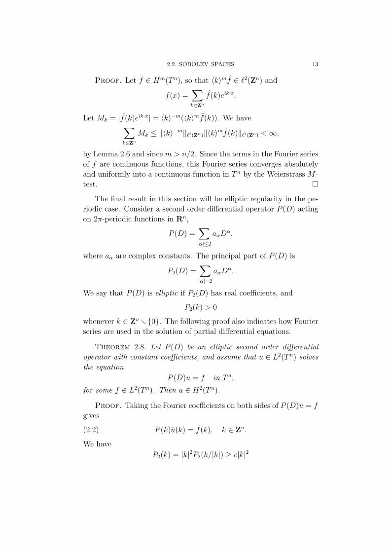
Proof. Let f ∈ Hm(T n), so that 〈k〉mf ∈ `2(Zn) and
f(x) =∑k∈Zn
f(k)eik·x.
Let Mk = |f(k)eik·x| = 〈k〉−m(〈k〉mf(k)). We have∑k∈Zn
Mk ≤ ‖〈k〉−m‖`2(Zn)‖〈k〉mf(k)‖`2(Zn) <∞,
by Lemma 2.6 and since m > n/2. Since the terms in the Fourier series
of f are continuous functions, this Fourier series converges absolutely
and uniformly into a continuous function in T n by the Weierstrass M -
test.
The final result in this section will be elliptic regularity in the pe-
riodic case. Consider a second order differential operator P (D) acting
on 2π-periodic functions in Rn,
P (D) =∑|α|≤2
aαDα,
where aα are complex constants. The principal part of P (D) is
P2(D) =∑|α|=2
aαDα.
We say that P (D) is elliptic if P2(D) has real coefficients, and
P2(k) > 0
whenever k ∈ Znr0. The following proof also indicates how Fourier
series are used in the solution of partial differential equations.
Theorem 2.8. Let P (D) be an elliptic second order differential
operator with constant coefficients, and assume that u ∈ L2(T n) solves
the equation
P (D)u = f in T n,
for some f ∈ L2(T n). Then u ∈ H2(T n).
Proof. Taking the Fourier coefficients on both sides of P (D)u = f
gives
(2.2) P (k)u(k) = f(k), k ∈ Zn.
We have
P2(k) = |k|2P2(k/|k|) ≥ c|k|2
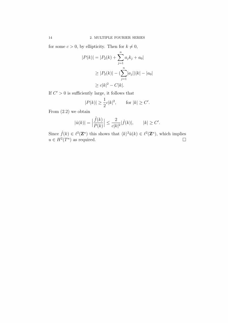
14 2. MULTIPLE FOURIER SERIES
for some c > 0, by ellipticity. Then for k 6= 0,
|P (k)| = |P2(k) +n∑j=1
ajkj + a0|
≥ |P2(k)| − (n∑j=1
|aj|)|k| − |a0|
≥ c|k|2 − C|k|.
If C ′ > 0 is sufficiently large, it follows that
|P (k)| ≥ 1
2c|k|2, for |k| ≥ C ′.
From (2.2) we obtain
|u(k)| =∣∣∣ f(k)
P (k)
∣∣∣ ≤ 2
c|k|2|f(k)|, |k| ≥ C ′.
Since f(k) ∈ `2(Zn) this shows that 〈k〉2u(k) ∈ `2(Zn), which implies
u ∈ H2(T n) as required.
CHAPTER 3
Uniqueness
In this chapter, we will discuss the proof of the following uniqueness
result of Sylvester and Uhlmann.
Theorem 3.1. Let Ω ⊆ Rn be a bounded open set with smooth
boundary, where n ≥ 3, and let γ1 and γ2 be two positive functions in
C2(Ω). If Λγ1 = Λγ2, then γ1 = γ2 in Ω.
In fact, this theorem will be reduced to a uniqueness result for the
Schrodinger equation (also due to Sylvester and Uhlmann).
Theorem 3.2. Let Ω ⊆ Rn be a bounded open set with smooth
boundary, where n ≥ 3, and let q1 and q2 be two functions in L∞(Ω)
such that the Dirichlet problems for −∆+q1 and −∆+q2 in Ω are well
posed. If Λq1 = Λq2, then q1 = q2 in Ω.
The reduction of Theorem 3.1 to Theorem 3.2 is presented in Sec-
tion 3.1 along with the relevant definitions. The proof of the uniqueness
results relies on complex geometrical optics (CGO) solutions, which
are constructed in Section 3.2 for the Schrodinger equation by Fourier
analysis and perturbation arguments. Section 3.3 includes an integral
identity relating boundary measurements to interior information about
the coefficients, and this identity is used to prove Theorem 3.2 by taking
an asymptotic limit with suitable CGO solutions.
3.1. Reduction to Schrodinger equation
The first step in the proof is the reduction of the conductivity equa-
tion to a Schrodinger equation,
(−∆ + q)u = 0 in Ω,
where q is a function in L∞(Ω). This equation turns out to be easier
to handle, since the principal part is the Laplacian −∆.
15
16 3. UNIQUENESS
Lemma 3.3. If γ ∈ C2(Ω) and u ∈ H1(Ω) then
(3.1) −∇ · γ∇(γ−1/2u) = γ1/2(−∆ + q)u
in the weak sense, where
q =∆√γ
√γ.
Proof. This is a direct computation: if u ∈ C2(Ω) then
− ∂j(γ∂j(1√γu)) = −∂j(
√γ∂ju) + ∂j(∂j(
√γ)u)
= −√γ∂2ju− ∂j(
√γ)∂ju+ ∂j(
√γ)∂ju+ ∂2
j (√γ)u.
The claim follows by taking the sum over j. The case where u ∈ H1(Ω)
can be proved by approximation1.
If q ∈ L∞(Ω), we consider the Dirichlet problem for the Schrodinger
equation,
(3.2)
(−∆ + q)u = 0 in Ω,
u = f on ∂Ω,
where f ∈ H1/2(∂Ω). We say that u ∈ H1(Ω) is a weak solution of
(3.2) if u|∂Ω = f , and if for all ϕ ∈ H10 (Ω) one has∫
Ω
(∇u · ∇ϕ+ quϕ) dx = 0.
1Let (uk) ⊆ C2(Ω) be a sequence with uk → u in H1(Ω). We have
−∇ · γ∇(γ−1/2uk) = γ1/2(−∆ + q)uk.
If a ∈ C1(Ω) then u 7→ au is a continuous map on H1(Ω), since
‖au‖H1(Ω) = ‖au‖L2(Ω)+‖(∇a)u+a∇u‖L2(Ω) ≤ 2(‖a‖L∞(Ω)+‖∇a‖L∞(Ω))‖u‖H1(Ω).
Using that γ is in C2(Ω) and that ∇ : Hm(Ω) → Hm−1(Ω) is a continuous map,we have
uk → u in H1(Ω)
=⇒ γ−1/2uk → γ−1/2u in H1(Ω)
=⇒ ∇(γ−1/2uk)→ ∇(γ−1/2u) in L2(Ω)
=⇒ γ∇(γ−1/2uk)→ γ∇(γ−1/2u) in L2(Ω)
=⇒ −∇ · γ∇(γ−1/2uk)→ −∇ · γ∇(γ−1/2u) in H−1(Ω).
Similarly, γ1/2(−∆ + q)uk → γ1/2(−∆ + q)u in H−1(Ω), which shows that (3.1)holds in the sense of H−1(Ω).
3.1. REDUCTION TO SCHRODINGER EQUATION 17
The problem (3.2) is said to be well-posed if the following three condi-
tions hold:
1. (existence) there is a weak solution u in H1(Ω) for any bound-
ary value f in H1/2(∂Ω),
2. (uniqueness) the solution u is unique,
3. (stability) the solution operator f 7→ u is continuous from
H1/2(∂Ω)→ H1(Ω), that is,
‖u‖H1(Ω) ≤ C‖f‖H1/2(∂Ω).
If the problem is well-posed, we can define a DN map formally by
Λq : H1/2(∂Ω)→ H−1/2(∂Ω), f 7→ ∂u
∂ν
∣∣∣∂Ω.
This is analogous to the conductivity equation, and also here the precise
definition of the DN map is given by the weak formulation
(Λqf, g)∂Ω =
∫Ω
(∇u · ∇v + quv) dx, f, g ∈ H1/2(∂Ω),
where u solves (3.2) and v is any function in H1(Ω) with v|∂Ω = g. The
next proof shows that this is a valid definition and Λq is a bounded
linear map.
Lemma 3.4. If q ∈ L∞(Ω) is such that the problem (3.2) is well-
posed, then Λq is a bounded linear map from H1/2(∂Ω) to H−1/2(∂Ω),
and satisfies
(Λqf, g)∂Ω = (f,Λqg)∂Ω, f, g ∈ H1/2(∂Ω).
Proof. Fix f ∈ H1/2(∂Ω), and define a map T : H1/2(∂Ω) → C
by
T (g) =
∫Ω
(∇u · ∇v + quv) dx,
where u solves (3.2) and v is any function in H1(Ω) with v|∂Ω = g.
Since u is a solution, we have∫Ω
(∇u · ∇ϕ+ quϕ) dx
for any ϕ ∈ H10 (Ω). Therefore we may replace v by v + ϕ in the
definition of T (g). If v, v ∈ H1(Ω) and v|∂Ω = v∂Ω = g, then v −v ∈ H1
0 (Ω), so indeed the definition does not depend on the particular
choice of v (as long as v ∈ H1(Ω) and v|∂Ω = g).
18 3. UNIQUENESS
Now, for g ∈ H1/2(∂Ω), use the one-sided inverse to the trace op-
erator to obtain vg ∈ H1(Ω) with ‖vg‖H1(Ω) ≤ C‖g‖H1/2(∂Ω). Then by
Cauchy-Schwarz
|T (g)| ≤∫
Ω
|∇u · ∇vg + quvg| dx ≤ C ′‖u‖H1(Ω)‖vg‖H1(Ω)
≤ C ′′‖f‖H1/2(∂Ω)‖g‖H1/2(∂Ω).
Thus T : H1/2(∂Ω)→ C is a continuous map, and there is an element
Λqf ∈ H−1/2(∂Ω) satisfying (Λqf, g) = T (g). Consequently, the map
Λq : f 7→ Λqf is a bounded linear map H1/2(∂Ω)→ H−1/2(∂Ω).
To show the last identity, let f, g ∈ H1/2(Ω), and let u, v be solutions
of (3.2) with boundary values u|∂Ω = f , v|∂Ω = g. Then
(Λqf, g)∂Ω =
∫Ω
(∇u · ∇v + quv) dx =
∫Ω
(∇v · ∇u+ qvu) dx = (Λqg, f)
by the definition of Λq.
The problem (3.2) is not always well-posed, consider for instance
the case q = −λ where λ > 0 is an eigenvalue of the Laplacian in Ω
(then there exists a nonzero u ∈ H1(Ω) with −∆u = λu in Ω and
u|∂Ω = 0). However, for potentials q coming from conductivities, the
Dirichlet problem is always well-posed, and there is a relation between
the DN maps Λγ and Λq.
Lemma 3.5. If γ ∈ C2(Ω) and q = ∆√γ/√γ, then the Dirichlet
problem (3.2) is well-posed and
Λqf = γ−1/2Λγ(γ−1/2f) +
1
2γ−1∂γ
∂νf∣∣∣∂Ω, f ∈ H1/2(Ω).
Proof. Fix f ∈ H1/2(∂Ω). We need to show that there is u in
H1(Ω) which solves (3.2). Motivated by Lemma 3.3, we take v be the
solution of ∇ · γ∇v = 0 in Ω with v|∂Ω = γ−1/2f . Then u = γ1/2v
is a function in H1(Ω) which solves (−∆ + q)u = 0 with the right
boundary values. The same argument with f = 0 shows that the
solution is unique. Further, since γ ∈ C2(Ω), we have the estimate
‖u‖H1(Ω) ≤ C‖v‖H1(Ω) ≤ C ′‖γ−1/2f‖H1/2(∂Ω) ≤ C ′′‖f‖H1/2(∂Ω).
If u solves (3.2), then v = γ−1/2u solves the conductivity equation
and
Λγ(γ−1/2f) = γ
∂v
∂ν= γ1/2∂u
∂ν− 1
2γ−1/2∂γ
∂νf.
3.1. REDUCTION TO SCHRODINGER EQUATION 19
Since Λqf = ∂u/∂ν, we obtain the relation between Λγ and Λq.
We may now show that uniqueness in the inverse conductivity prob-
lem can be deduced from the corresponding result for the Schrodinger
equation.
Proof that Theorem 3.2 implies Theorem 3.1. Let γ1, γ2 be
positive functions in C2(Ω), and assume that Λγ1 = Λγ2 . If qj =
∆√γj/√γj, then qj ∈ L∞(Ω) and by Theorem 3.5 the Dirichlet prob-
lems for −∆ + qj are well posed. Also, the boundary reconstruction
result ([5], Theorem 6.6.1) implies that γ1 = γ2 and ∂γ1/∂ν = ∂γ2/∂ν
on ∂Ω. Thus, for any f in H1/2(∂Ω) one has
Λq1f = γ−1/21 Λγ1(γ
−1/21 f) +
1
2γ−1
1
∂γ1
∂νf∣∣∣∂Ω
= γ−1/22 Λγ2(γ
−1/22 f) +
1
2γ−1
2
∂γ2
∂νf∣∣∣∂Ω
= Λq2f.
Theorem 3.2 gives that q1 = q2 in Ω. Therefore,
(3.3)∆√γ1√γ1
=∆√γ2√γ2
in Ω.
We would like to conclude from (3.3) that γ1 = γ2. Let q =
γ−1/21 ∆γ1 = γ
−1/22 ∆γ2, and consider the equation
(−∆ + q)u = 0 in Ω.
Both√γ1 and
√γ2 solve this equation, and
√γ1|∂Ω =
√γ2|∂Ω by bound-
ary determination. Since the Schrodinger equation with potential q
coming from a conductivity is well-posed, we obtain γ1 = γ2 by unique-
ness of solutions.
Remark 3.6. We record for later use another argument showing
that (3.3) implies γ1 = γ2. The equation (3.3) looks like a nonlinear
PDE involving γ1 and γ2. To simplify the equation, we note that
∆(log√γ) =
n∑j=1
∂j(1√γ∂j√γ) =
∆√γ
√γ− |∇(log
√γ)|2.
The equation becomes
∆(log√γ1 − log
√γ2) + |∇(log
√γ1)|2 − |∇(log
√γ2)|2 = 0.
20 3. UNIQUENESS
Rewriting slightly, we get
∆(log
√γ1√γ2
) +∇a · ∇(log
√γ1√γ2
) = 0,
where a = log√γ1γ2. This is a linear equation for the C2 function
v = log√γ1√γ2
. Further, noting the identity
∇ · (ea∇v) = ea(∆v +∇a · ∇v),
and using the fact that γ1 = γ2 on ∂Ω, we see that v solves the Dirichlet
problem ∇ · ((γ1γ2)1/2∇v) = 0 in Ω,
v = 0 on ∂Ω.
This problem is well-posed, and we get v ≡ 0 and γ1 ≡ γ2.
3.2. Complex geometrical optics
In this section, we will construct complex geometrical optics (CGO)
solutions to the Schrodinger equation
(−∆ + q)u = 0 in Ω.
The potential q is assumed to be in L∞(Ω).
Motivation. First let q = 0. We try as a solution to the equation
−∆u = 0 the complex exponential at frequency ζ ∈ Cn,
u(x) = eiζ·x.
This satisfies
Du(x) = ζeiζ·x, D2u(x) = (ζ · ζ)eiζ·x.
Thus, if ζ ∈ Cn satisfies ζ · ζ = 0, then u(x) = eiζ·x solves −∆u = 0.
Writing ζ = Re ζ + i Im ζ, we see that
ζ · ζ = 0 ⇐⇒ |Re ζ| = |Im ζ|, Re ζ · Im ζ = 0.
Now suppose q is nonzero. The function u = eiζ·x is not an exact
solution of (−∆ + q)u = 0 anymore, but we can find solutions which
resemble complex exponentials. These are the CGO solutions, which
have the form
(3.4) u(x) = eiζ·x(1 + r(x)).
Here r is a correction term which is needed to convert the approximate
solution eiζ·x to an exact solution.
3.2. COMPLEX GEOMETRICAL OPTICS 21
In fact, we are interested in solutions in the asymptotic limit as
|ζ| → ∞. This follows the principle that it is usually not possible
to obtain explicit formulas for solutions to general equations, but in
suitable asymptotic limits explicit expressions for solutions may exist.
We note that (3.4) is a solution of (−∆ + q)u = 0 iff
(3.5) e−iζ·x(−∆ + q)eiζ·x(1 + r) = 0.
It will be convenient to conjugate the exponentials eiζ·x into the Lapla-
cian. By this we mean that
e−iζ·xDj(eiζ·xv) = (Dj + ζj)v,
e−iζ·xD2(eiζ·xv) = (D + ζ)2v = (D2 + 2ζ ·D)v.
We can rewrite (3.5) as
(D2 + 2ζ ·D + q)(1 + r) = 0.
This implies the following equation for r:
(3.6) (D2 + 2ζ ·D + q)r = −q.
The solvability of (3.6) is the most important step in the construction
of CGO solutions. We proceed in several steps.
3.2.1. Basic estimate. We first consider the free case in which
there is no potential on the left hand side of (3.6).
Theorem 3.7. There is a constant C0 depending only on Ω and n,
such that for any ζ ∈ Cn satisfying ζ · ζ = 0 and |ζ| ≥ 1, and for any
f ∈ L2(Ω), the equation
(3.7) (D2 + 2ζ ·D)r = f in Ω
has a solution r ∈ H1(Ω) satisfying
‖r‖L2(Ω) ≤C0
|ζ|‖f‖L2(Ω),
‖∇r‖L2(Ω) ≤ C0‖f‖L2(Ω).
The idea of the proof is that (3.7) is a linear equation with constant
coefficients, so one can try to solve it by the Fourier transform. Since
(Dju) (ξ) = ξju(ξ), the Fourier transformed equation is
(ξ2 + 2ζ · ξ)r(ξ) = f(ξ).
22 3. UNIQUENESS
We would like to divide by ξ2 + 2ζ · ξ and use the inverse Fourier
transform to get a solution r. However, the symbol ξ2 + 2ζ · ξ vanishes
for some ξ ∈ Rn, and the division cannot be done directly.
It turns out that we can divide by the symbol if we use Fourier
series in a large cube instead of the Fourier transform, and moreover
take the Fourier coefficients in a shifted lattice instead of the usual
integer coordinate lattice.
Proof of Theorem 3.7. Write ζ = s(ω1+iω2) where s = |ζ|/√
2
and ω1 and ω2 are orthogonal unit vectors in Rn. By rotating coor-
dinates in a suitable way, we can assume that ω1 = e1 and ω2 = e2
(the first and second coordinate vectors). Thus we need to solve the
equation
(D2 + 2s(D1 + iD2))r = f.
We assume for simplicity that Ω is contained in the cube Q =
[−π, π]n. Extend f by zero outside Ω into Q, which gives a function in
L2(Q) also denoted by f . We need to solve
(3.8) (D2 + 2s(D1 + iD2))r = f in Q.
Let wk(x) = ei(k+ 12e2)·x for k ∈ Zn. That is, we consider Fourier series
in the lattice Zn + 12e2. Writing
(u, v) = (2π)−n∫Q
uv dx, u, v ∈ L2(Q),
we see that (wk, wl) = 0 if k 6= l and (wk, wk) = 1, so wk is an
orthonormal set in L2(Q). It is also complete: if v ∈ L2(Q) and
(v, wk) = 0 for all k ∈ Zn then (ve−12ix2 , eik·x) = 0 for all k ∈ Zn,
which implies v = 0.
Hilbert space theory gives that f can be written as the series f =∑k∈Zn fkwk, where fk = (f, wk) and ‖f‖2
L2(Q) =∑
k∈Zn|fk|2. Seeking
also r in the form r =∑
k∈Zn rkwk, and using that
Dwk = (k +1
2e2)wk,
the equation (3.8) results in
pkrk = fk, k ∈ Zn,
where
pk := (k +1
2e2)2 + 2s(k1 + i(k2 +
1
2)).
3.2. COMPLEX GEOMETRICAL OPTICS 23
Note that Im pk = 2s(k2 + 12) is never zero, which was the reason for
considering the shifted lattice. We define
rk :=1
pkfk
and
r :=∑k∈Zn
rkwk.
The last series converges in L2(Q) to a function r ∈ L2(Q) since
|rk| ≤1
|pk||fk| ≤
1
|2s(k2 + 12)||fk| ≤
1
s|fk|,
and then
‖r‖L2(Q) =(∑
k
|rk|2)1/2
≤ 1
s
(∑k
|fk|2)1/2
=1
s‖f‖L2(Q).
This shows the desired estimate in L2(Q).
It remains to show that Dr ∈ L2(Q) with correct bounds. We have
Dr =∑k∈Zn
(k +1
2e2)rkwk.
The derivative is justified since this is a convergent series in L2(Q): we
claim
(3.9) |(k +1
2e2)rk| ≤ 4|fk|, k ∈ Zn,
which implies that ‖Dr‖L2(Q) ≤ 4‖f‖L2(Q). To show (3.9) we consider
two cases: if |k + 12e2| ≤ 4s we have
|(k +1
2e2)rk| ≤
4s
2s|k2 + 1/2||fk| ≤ 4|fk|,
and if |k + 12e2| ≥ 4s then
||k +1
2e2|2 + 2sk1| ≥ |k +
1
2e2|2 − 2s|k +
1
2e2| ≥
1
2|k +
1
2e2|2
which implies
|(k +1
2e2)rk| ≤
|k + 12e2|
12|k + 1
2e2|2|fk| ≤
1
2s|fk|.
The statement is proved.
24 3. UNIQUENESS
3.2.2. Basic estimate with potential. Now we consider the so-
lution of (3.6) in the presence of a nonzero potential. It will be conve-
nient to give a name to the solution operator in the free case.
Notation. Let ζ ∈ Cn satisfy ζ · ζ = 0 and |ζ| sufficiently large.
We denote by Gζ the solution operator
Gζ : L2(Ω)→ H1(Ω), f 7→ r,
where r is the solution to (D2 + 2ζ ·D)r = f provided by Theorem 3.7.
Theorem 3.8. Let q ∈ L∞(Ω). There is a constant C0 depending
only on Ω and n, such that for any ζ ∈ Cn satisfying ζ · ζ = 0 and
|ζ| ≥ max(C0‖q‖L∞(Ω), 1), and for any f ∈ L2(Ω), the equation
(3.10) (D2 + 2ζ ·D + q)r = f in Ω
has a solution r ∈ H1(Ω) satisfying
‖r‖L2(Ω) ≤C0
|ζ|‖f‖L2(Ω),
‖∇r‖L2(Ω) ≤ C0‖f‖L2(Ω).
Proof. If one has q = 0, a solution would be given by r = Gζf .
Here q may be nonzero, so we try a solution of the form
(3.11) r := Gζ f ,
where f ∈ L2(Ω) is a function to be determined. Inserting (3.11) in
the equation (3.10), and using that (D2 + 2ζ ·D)Gζ = I, we see that f
should satisfy
(3.12) (I + qGζ)f = f in Ω.
We have the norm estimate
‖qGζ‖L2(Ω)→L2(Ω) ≤C0‖q‖L∞(Ω)
|ζ|.
If |ζ| ≥ max(2C0‖q‖L∞(Ω), 1) then
‖qGζ‖L2(Ω)→L2(Ω) ≤1
2.
It follows that I + qGζ is an invertible operator on L2(Ω), and the
equation (3.12) has a solution
f := (I + qGζ)−1f.
3.2. COMPLEX GEOMETRICAL OPTICS 25
The definition (3.11) for r implies
(D2 + 2ζ ·D + q)r = f + qGζ f = (I + qGζ)f = f,
and r indeed solves the equation (3.10). Since ‖(I+qGζ)−1‖L2(Ω)→L2(Ω) ≤
2, we have ‖f‖L2(Ω) ≤ 2‖f‖L2(Ω). The norm estimates in Theorem 3.7
imply the desired estimates for r, if we replace C0 by 2C0.
3.2.3. Construction of CGO solutions. It is now easy to give
the main result on the existence of CGO solutions. Note that the
constant function a ≡ 1 always satisfies ζ · ∇a = 0, so as a special case
one obtains the solutions u = eiζ·x(1 + r) in (3.4).
Theorem 3.9. Let q ∈ L∞(Ω). There is a constant C0 depending
only on Ω and n, such that for any ζ ∈ Cn satisfying ζ · ζ = 0 and
|ζ| ≥ max(C0‖q‖L∞(Ω), 1), and for any function a ∈ H2(Ω) satisfying
ζ · ∇a = 0 in Ω,
the equation (−∆ + q)u = 0 in Ω has a solution
(3.13) u(x) = eiζ·x(a+ r),
where r ∈ H1(Ω) satisfies
‖r‖L2(Ω) ≤C0
|ζ|‖(−∆ + q)a‖L2(Ω),
‖∇r‖L2(Ω) ≤ C0‖(−∆ + q)a‖L2(Ω).
Proof. The function (3.13) is a solution of (−∆ + q)u = 0 iff
(3.14) e−iζ·x(−∆ + q)eiζ·x(a+ r) = 0.
As in the beginning of this section, we conjugate the exponentials into
the derivatives and rewrite (3.5) as
(D2 + 2ζ ·D + q)(a+ r) = 0.
Since ζ ·Da = 0, this implies the following equation for r:
(D2 + 2ζ ·D + q)r = −(D2 + q)a.
Theorem 3.8 guarantees the existence of a solution r satisfying the norm
estimates above. Then (3.13) is the required solution to (−∆+q)u = 0
in Ω.
26 3. UNIQUENESS
3.3. Uniqueness proof
In this section we prove the Sylvester-Uhlmann uniqueness results.
As shown in Section 3.1, uniqueness in the inverse conductivity problem
(Theorem 3.1) follows from the uniqueness result for the Schrodinger
equation, which we now recall.
Theorem 3.2. Let Ω ⊆ Rn be a bounded open set with smooth
boundary, where n ≥ 3, and let q1 and q2 be two functions in L∞(Ω)
such that the Dirichlet problems for −∆+q1 and −∆+q2 in Ω are well
posed. If Λq1 = Λq2, then q1 = q2 in Ω.
The starting point is an integral identity which relates the differ-
ence of the boundary measurements Λq1 − Λq2 to the difference of the
potentials.
Lemma 3.8. Let q1 and q2 be two functions in L∞(Ω) such that the
Dirichlet problems for −∆ + q1 and −∆ + q2 in Ω are well-posed. Then
for any f1, f2 ∈ H1/2(∂Ω) one has
〈(Λq1 − Λq2)f1, f2〉 =
∫Ω
(q1 − q2)u1u2 dx,
where uj ∈ H1(Ω) is the solution of (−∆+qj)uj = 0 in Ω with boundary
values uj|∂Ω = fj, j = 1, 2.
Proof. By the weak definition of the DN map, we have
〈Λq1f1, f2〉 =
∫Ω
(∇u1 · ∇u2 + q1u1u2) dx
since u1 is a solution with boundary values f1, and u2 has boundary
values f2. Also, since the DN map is self-adjoint,
〈Λq2f1, f2〉 = 〈f1,Λq2f2〉 = 〈Λq2f2, f1〉 =
∫Ω
(∇u2 · ∇u1 + q2u2u1) dx.
The claim follows.
Proof of Theorem 3.2. Since Λq1 = Λq2 , we know from Lemma
3.8 that
(3.15)
∫Ω
(q1 − q2)u1u2 dx = 0
for any H1 solutions uj to the equations (−∆ + qj)uj = 0, j = 1, 2.
Thus, to prove that q1 = q2, it is enough to establish that products
u1u2 of such solutions are dense in L1(Ω).
3.3. UNIQUENESS PROOF 27
Fix ξ ∈ Rn. We would like to choose the solutions in such a way
that u1u2 is close to eix·ξ, since the functions eix·ξ form a dense set. We
begin by taking unit vectors ω1 and ω2 in Rn such that ω1, ω2, ξ is
an orthogonal set (here we need that n ≥ 3). Let
ζ = s(ω1 + iω2),
so that ζ · ζ = 0. By Theorem 3.9, if s is sufficiently large there exist
H1 solutions u1 and u2 which satisfy (−∆ + qj)uj = 0, and which are
of the form
u1 = eiζ·x(eix·ξ + r1),
u2 = e−iζ·x(1 + r2),
where ‖rj‖L2(Ω) ≤ C/s for j = 1, 2. For the first solution we chose
a = eix·ξ which satisfies ζ · ∇a = (ζ · ξ)eix·ξ = 0 by orthogonality, and
for the second solution we chose a to be constant.
Inserting these solutions in (3.15), we obtain
(3.16)
∫Ω
(q1 − q2)(eix·ξ + r1)(1 + r2) dx = 0.
In this identity, only r1 and r2 depend on s. Since the L2 norms of r1
and r2 are bounded by C/s, it is possible to take the limit as s → ∞in (3.15), and then the terms involving r1 and r2 will vanish. Taking
this limit in (3.16), we get∫Ω
(q1 − q2)eix·ξ dx = 0.
This holds for every ξ ∈ Rn. If q is the function in L1(Rn) which is
equal to q1 − q2 in Ω and vanishes outside Ω, the last identity implies
that the Fourier transform of q vanishes for every frequency ξ ∈ Rn.
Consequently q = 0, and q1 = q2 in Ω.

CHAPTER 4
Stability
In the preceding chapter, we proved that if γ1, γ2 are two conduc-
tivities in C2(Ω) such that Λγ1 is equal to Λγ2 , then γ1 ≡ γ2. Here we
address the stability question: if γ1, γ2 are two conductivities such that
Λγ1 is close to Λγ2 , does this imply that γ1 is close to γ2?
More precisely, we are looking for an estimate of the form
(4.1) ‖γ1 − γ2‖L∞(Ω) ≤ ω(‖Λγ1 − Λγ2‖∗),
where ‖ · ‖∗ = ‖ · ‖H1/2(∂Ω)→H−1/2(∂Ω) is the natural operator norm for
the DN maps, and ω : [0,∞)→ [0,∞) is a modulus of continuity, that
is, a continuous nondecreasing function satisfying ω(t)→ 0 as t→ 0+.
We begin with an example due to Alessandrini.
Example. Let D be the unit disc in R2, and let γ1, γ2 ∈ L∞(D) be
two conductivities such that γ1 ≡ 1 in D, and
γ2(x) =
1 + A, |x| < r0,
1, r0 < |x| < 1,
where A is a positive constant and r0 ∈ (0, 1). If f ∈ H1/2(∂D), then
f may be written as Fourier series
f(eiθ) =∞∑
k=−∞
f(k)eikθ.
It can be shown (exercise) that
Λγ1f(eiθ) =∞∑
k=−∞
|k|f(k)eikθ,
Λγ2f(eiθ) =∞∑
k=−∞
|k|2 + A(1 + r2|k|0 )
2 + A(1− r2|k|0 )
f(k)eikθ.
29
30 4. STABILITY
Then
‖(Λγ1−Λγ2)f‖2H−1/2 =
∞∑k=−∞
(1+k2)−1/2k2
∣∣∣∣∣1−2 + A(1 + r2|k|0 )
2 + A(1− r2|k|0 )
2∣∣∣∣∣2
|f(k)|2
=∞∑
k=−∞
k2
1 + k2
(2Ar
2|k|0
2 + A(1− r2|k|0 )
)2
(1 + k2)1/2|f(k)|2.
The sum is actually over k 6= 0, and then the expression in parentheses
is ≤ Ar20 since it attains its maximum value when |k| = 1. It follows
that
‖Λγ1 − Λγ2‖∗ = sup‖f‖
H1/2=1
‖(Λγ1 − Λγ2)f‖H−1/2 ≤ Ar20.
Now ‖Λγ1 − Λγ2‖∗ → 0 as r0 → 0, but
‖γ1 − γ2‖L∞(D) = A.
Thus, an estimate of the form (4.1) can not be valid if one only assumes
that γ1, γ2 ∈ L∞.
It turns out that under certain a priori assumptions on γ1 and γ2,
it is possible to prove a stability estimate with logarithmic modulus of
continuity.
Theorem 4.1. Let Ω ⊆ Rn be a bounded open set with smooth
boundary, where n ≥ 3, and let γj, j = 1, 2, be two positive functions
in Hs+2(Ω) with s > n/2, satisfying
1M≤ γj ≤M,(4.2)
‖γj‖Hs+2(Ω) ≤M.(4.3)
There are constants C = C(Ω, n,M, s) > 0 and σ = σ(n, s) ∈ (0, 1)
such that
‖γ1 − γ2‖L∞(Ω) ≤ ω(‖Λγ1 − Λγ2‖∗)where ω is a modulus of continuity satisfying
ω(t) ≤ C|log t|−σ, 0 < t < 1/e.
Note that γj ∈ Hs+2(Ω) with s > n/2 implies that γj ∈ C2(Ω) by
Sobolev embedding. The logarithmic modulus of continuity is rather
weak, in the sense that even small changes in γ can result in large
changes in Λγ. However, it has been proved that the logarithmic mod-
ulus is optimal, and for instance Holder type stability can not hold for
conductivities of general form.
4.1. SCHRODINGER EQUATION 31
4.1. Schrodinger equation
As in the uniqueness proof, we will use the inverse problem for the
Schrodinger equation to study the stability question. In the following,
Ω ⊆ Rn is a bounded open set with C∞ boundary, and n ≥ 3.
Theorem 4.2. Let qj ∈ L∞(Ω) be two potentials such that the
Dirichlet problems for −∆ + qj are well-posed. Further, assume that
‖qj‖L∞(Ω) ≤M.
There is a constant C = C(Ω, n,M) such that
‖q1 − q2‖H−1(Ω) ≤ ω(‖Λq1 − Λq2‖∗)
where ω is a modulus of continuity satisfying
ω(t) ≤ C|log t|−2
n+2 , 0 < t < 1/e.
Proof. Let ξ ∈ Rn. We start from the identity in Lemma 3.8,
which states that
(4.4)
∫Ω
(q1 − q2)u1u2 dx = ((Λq1 − Λq2)(u1|∂Ω), u2|∂Ω)∂Ω,
for any uj ∈ H1(Ω) which solve (−∆ + qj)uj = 0 in Ω. As in the proof
of Theorem 3.2, let ω1 and ω2 be unit vectors such that ω1, ω2, ξ is
an orthogonal set. The choice of complex vectors is slightly different
(we make this choice to obtain better constants), we take
ζ1 =s√2
(
√1− |ξ|
2
2s2ω1 +
1√2sξ + iω2),
ζ2 = − s√2
(
√1− |ξ|
2
2s2ω1 −
1√2sξ + iω2).
These satisfy ζj · ζj = 0 and |ζ1| = |ζ2| = s. Theorem 3.9 ensures
the existence of solutions uj to (−∆ + qj)uj = 0, provided that s ≥max(C0M, 1), of the form
u1 = eiζ1·x(1 + r1),
u2 = eiζ2·x(1 + r2),
with ‖rj‖L2(Ω) ≤ C0‖qj‖L∞s
, and C0 = C0(Ω, n).
32 4. STABILITY
Inserting u1 and u2 in (4.4) and using that ei(ζ1+ζ2)·x = eix·ξ, we
obtain∣∣∣ ∫Ω
(q1 − q2)eix·ξ dx∣∣∣ ≤ ‖Λq1 − Λq2‖∗‖u1‖H1/2(∂Ω)‖u2‖H1/2(∂Ω)
+∣∣∣ ∫
Ω
(q1 − q2)eix·ξ(r1 + r2 + r1r2) dx∣∣∣
≤ ‖Λq1 − Λq2‖∗‖u1‖H1‖u2‖H1 + C(‖r1‖L2 + ‖r2‖L2 + ‖r1‖L2‖r2‖L2)
with C = C(Ω, n,M). If Ω ⊆ B(0, R) then
‖uj‖H1 ≤ ‖eiζj ·x(1 + rj)‖L2 +n∑k=1
‖∂k(eiζj ·x)(1 + rj) + eiζj ·x∂krj‖L2
≤ CseRs.
We assume that s is so large that s ≤ eRs, and have
(4.5) |(q1 − q2) (ξ)| ≤ C(e4Rs‖Λq1 − Λq2‖∗ +
1
s
),
where qj is the extension of qj to Rn by zero (thus qj ∈ L1(Rn)).
So far, we have proved that there are constants C and C ′, depending
on Ω, n, and M , such that (4.5) holds whenever s ≥ C ′. It is possible
to obtain a bound for q1− q2 in H−1 by using (4.5) and the L∞ bounds
for qj. If ρ > 0 is a constant which will be determined later, we have
‖q1−q2‖2H−1(Ω) ≤ ‖q1−q2‖2
H−1(Rn) =(∫|ξ|≤ρ
+
∫|ξ|>ρ
) |(q1 − q2) (ξ)|2
1 + |ξ|2dξ
≤ Cρn(e8Rs‖Λq1 − Λq2‖2
∗ +1
s2
)+ (1 + ρ2)−1‖q1 − q2‖2
L2(Rn)
≤ Cρne8Rs‖Λq1 − Λq2‖2∗ +
Cρn
s2+C
ρ2.
To make the last two terms of equal size, we choose
ρ = s2
n+2 .
Then
‖q1 − q2‖2H−1(Ω) ≤ Ce16Rs‖Λq1 − Λq2‖2
∗ + Cs−4
n+2
for s ≥ C ′(Ω, n,M). We make the final choice
s =1
16R|log‖Λq1 − Λq2‖∗|
4.2. MORE FACTS ON SOBOLEV SPACES 33
where we assume that
0 < ‖Λq1 − Λq2‖∗ < c′(Ω, n,M)
with c′ chosen so that s ≥ C ′. With this assumption, it follows that
‖q1 − q2‖2H−1(Ω) ≤ C(‖Λq1 − Λq2‖∗ + |log‖Λq1 − Λq2‖∗|−
4n+2 ).
The claim is an easy consequence.
4.2. More facts on Sobolev spaces
To reduce the stability result for the conductivity equation to The-
orem 4.2, we will need more properties of Sobolev spaces. There
are three settings to consider: Sobolev spaces in Rn, Sobolev spaces
in bounded C∞ domains Ω ⊆ Rn, and Sobolev spaces on (n − 1)-
dimensional boundaries ∂Ω. Further, we want to consider the case
where s may not be an integer.
The philosophy is thatHs(Rn) may be defined via the Fourier trans-
form, Hs(Ω) is the restriction of Hs(Rn) to Ω, and Hs(∂Ω) can be
defined by locally flattening the boundary and reducing matters to
Hs(Rn−1). We now give some specifics, see [7] for more details.
Definition. If s ≥ 0, let
Hs(Rn) = u ∈ L2(Rn) ; 〈ξ〉su(ξ) ∈ L2(Rn),
with norm
‖u‖Hs(Rn) = ‖〈ξ〉su‖L2(Rn).
Here 〈ξ〉 = (1 + |ξ|2)1/2 for ξ ∈ Rn.
The space Hs(Rn) is in fact a Hilbert space, with inner product
(u, v)Hs =∫〈ξ〉2su(ξ)v(ξ). Recall from [5] that if k ≥ 0 is an integer,
there is the equivalent norm
(4.6) ‖u‖Wk,2(Rn) :=∑|α|≤k
‖∂αu‖L2(Rn) ∼ ‖u‖Hk(Rn),
where A ∼ B means that c−1B ≤ A ≤ cB for some constant c > 0
(independent of u).
The following properties of Sobolev spaces are the main point in
this section. Recall that Ck(Rn) is the space of k times continuously
differentiable functions on Rn, such that all partial derivatives up to
order k are bounded. The norm is ‖u‖Ck(Rn) =∑|α|≤k‖∂αu‖L∞(Rn).
34 4. STABILITY
Theorem 4.3.
• (Sobolev embedding theorem) If u ∈ Hs+k(Rn) where s > n/2
and k is a nonnegative integer, then u ∈ Ck(Rn) and
‖u‖Ck(Rn) ≤ C‖u‖Hs+k(Rn).
• (Multiplication by functions) If u ∈ Hs(Rn) and s ≥ 0, and if
f ∈ Ck(Rn) where k is an integer ≥ s, then fu ∈ Hs(Rn) and
‖fu‖Hs(Rn) ≤ ‖f‖Ck(Rn)‖u‖Hs(Rn).
• (Logarithmic convexity of Sobolev norms) If 0 ≤ α ≤ β and
0 ≤ t ≤ 1, then
‖u‖Hγ(Rn) ≤ ‖u‖1−tHα(Rn)‖u‖
tHβ(Rn), u ∈ Hβ(Rn),
where γ = (1− t)α + tβ.
Proof. The first statement was proved in [5]. The second fact
follows, if s is an integer, by using the equivalent norm (4.6) and the
Leibniz rule. If s is not an integer, the most convenient way to prove
the result is by interpolation: if s = l − ε where l is an integer and
0 < ε < 1, the claim is true if s is replaced by l− 1 or l, and the claim
follows for s by interpolation between these two cases.
We now prove the third statement. The claim is trivial if t = 0 or
t = 1, so assume that 0 < t < 1. Then
‖u‖2Hγ(Rn) =
∫〈ξ〉2((1−t)α+tβ)|u(ξ)|2 dξ
=
∫(〈ξ〉2α|u(ξ)|2)1−t(〈ξ〉2β|u(ξ)|2)t dξ
≤(∫〈ξ〉2α|u(ξ)|2 dξ
)1−t(∫〈ξ〉2β|u(ξ)|2 dξ
)t= ‖u‖2(1−t)
Hα(Rn)‖u‖2tHβ(Rn)
by using Holder’s inequality with p = 11−t and p′ = 1
t.
We would like to use similar results for Sobolev spaces in bounded
domains. In the following, let Ω ⊆ Rn be a bounded open set with
C∞ boundary. In [5] one has the Sobolev spaces in Ω, denoted here by
W k,2(Ω), consisting of the functions in L2(Ω) whose all weak partial
derivatives up to order k are in L2(Ω). The norm is
‖u‖Wk,2(Ω) :=∑|α|≤k
‖∂αu‖L2(Ω).
4.2. MORE FACTS ON SOBOLEV SPACES 35
We wish to relate these to Sobolev spaces in Rn. The main tool for
doing this is the extension operator.
Theorem 4.4. (Extension operator) If k is a nonnegative integer,
there is a bounded linear operator E : W k,2(Ω) → Hk(Rn) satisfying
Eu|Ω = u.
Proof. See the exercises.
Definition. If s ≥ 0, let Hs(Ω) be the set of those u ∈ L2(Ω) such
that u = v|Ω for some v ∈ Hs(Rn). The norm is the quotient norm
‖u‖Hs(Ω) = infv∈Hs(Rn),v|Ω=u
‖v‖Hs(Rn).
The space Hs(Ω) is a Hilbert space. The definition is justified by
the fact that
Hk(Ω) = W k,2(Ω),
with equivalent norms, if k ≥ 0 is an integer. To see this, note that
‖u‖Hk(Ω) ≤ ‖Eu‖Hk(Rn) ≤ C‖u‖Wk,2(Ω).
Further, if u ∈ W k,2(Ω) and if v ∈ Hk(Rn) with v|Ω = u, then
‖u‖Wk,2(Ω) ≤ ‖v‖Wk,2(Rn). Therefore
‖u‖Wk,2(Ω) ≤ C‖u‖Hk(Ω).
On domains, the following results correspond to the ones above.
Theorem 4.5.
• (Sobolev embedding theorem) If u ∈ Hs+k(Ω) where s > n/2
and k is a nonnegative integer, then u ∈ Ck(Ω) and
‖u‖Ck(Ω) ≤ C‖u‖Hs+k(Ω).
• (Multiplication by functions) If u ∈ Hs(Ω) and s ≥ 0, and if
f ∈ Ck(Ω) where k is an integer ≥ s, then fu ∈ Hs(Ω) and
‖fu‖Hs(Ω) ≤ ‖f‖Ck(Ω)‖u‖Hs(Ω).
• (Logarithmic convexity of Sobolev norms) If 0 ≤ α ≤ β and
0 ≤ t ≤ 1, then
‖u‖H(1−t)α+tβ(Ω) ≤ ‖u‖1−tHα(Ω)‖u‖
tHβ(Ω), u ∈ Hβ(Ω).
36 4. STABILITY
Proof. The first item follows from the corresponding result on Rn
by using the extension operator: if u ∈ Hs+k(Ω), there is v ∈ Hs+k(Rn)
with v|Ω = u and ‖v‖Hs+k(Rn) ≤ C‖u‖Hs+k(Ω). Sobolev embedding in
Rn implies v ∈ Ck(Rn) with ‖v‖Ck(Rn) ≤ C‖v‖Hs+k(Rn). Then
‖u‖Ck(Ω) ≤ ‖v‖Ck(Rn) ≤ C‖v‖Hs+k(Rn) ≤ C‖u‖Hs+k(Ω).
The second item is again a direct computation for integer s and in
general can be proved by interpolation, and this is also true for the
third item.
Next consider the spaces Hs(∂Ω), where ∂Ω is the boundary of a
bounded C∞ domain Ω. As described in [5], one can define Hs(∂Ω) via
the spaces Hs(Rn−1), by using a partition of unity and diffeomorphisms
which locally flatten the boundary. The above properties carry over to
the spaces Hs(∂Ω). Note that in the Sobolev embedding theorem, the
condition is s > n−12
since ∂Ω is an (n− 1)-dimensional manifold.
Theorem 4.6.
• (Sobolev embedding theorem) If u ∈ Hs+k(∂Ω) where s > n−12
and k is a nonnegative integer, then u ∈ Ck(∂Ω) and
‖u‖Ck(∂Ω) ≤ C‖u‖Hs+k(∂Ω).
• (Multiplication by functions) If u ∈ Hs(∂Ω) and s ≥ 0, and if
f ∈ Ck(∂Ω) where k is an integer ≥ s, then fu ∈ Hs(∂Ω) and
‖fu‖Hs(∂Ω) ≤ ‖f‖Ck(∂Ω)‖u‖Hs(∂Ω).
• (Logarithmic convexity of Sobolev norms) If 0 ≤ α ≤ β and
0 ≤ t ≤ 1, then
‖u‖H(1−t)α+tβ(∂Ω) ≤ ‖u‖1−tHα(∂Ω)‖u‖
tHβ(∂Ω), u ∈ Hβ(∂Ω).
Finally, a remark about negative index Sobolev spaces Hs(Rn),
Hs(Ω), Hs(∂Ω), where s < 0. These spaces contain elements which are
no longer L2 functions, and in fact are not functions at all. The most
convenient definition uses the space of tempered distributions S ′(Rn),
which contains for instance all Lp functions and polynomially bounded
measures, and which is closed under the Fourier transform. Then, if
s ∈ R, one defines
Hs(Rn) = u ∈ S ′(Rn) ; 〈ξ〉su(ξ) ∈ L2(Rn),‖u‖Hs(Rn) = ‖〈ξ〉su(ξ)‖L2(Rn).

4.3. CONDUCTIVITY EQUATION 37
Further, Hs(Ω) can be defined via restriction as above, and Hs(∂Ω) by
reducing to Hs(Rn−1). We will use the fact that multiplication by Ck
functions is bounded on Hs for |s| ≤ k, which can be proved by duality
arguments.
4.3. Conductivity equation
We proceed to prove the main result on stability for the conductivity
equation, which we recall here.
Theorem 4.1. Let Ω ⊆ Rn be a bounded open set with smooth
boundary, where n ≥ 3, and let γj, j = 1, 2, be two positive functions
in Hs+2(Ω) with s > n/2, satisfying
1M≤ γj ≤M,(4.7)
‖γj‖Hs+2(Ω) ≤M.(4.8)
There are constants C = C(Ω, n,M, s) > 0 and σ = σ(n, s) ∈ (0, 1)
such that
‖γ1 − γ2‖L∞(Ω) ≤ ω(‖Λγ1 − Λγ2‖∗)where ω is a modulus of continuity satisfying
ω(t) ≤ C|log t|−σ, 0 < t < 1/e.
The proof will involve a stability result at the boundary. This is an
easier problem, and in fact one has stability with a Lipschitz modulus
of continuity.
Theorem 4.7. (Boundary stability) Under the assumptions in The-
orem 4.1, one has
‖γ1 − γ2‖L∞(∂Ω) ≤ C‖Λγ1 − Λγ2‖∗where C = C(Ω, n,M, s).
Proof. Follows by using the same method as in the proof of the
boundary determination result in [5], see the exercises.
We need to relate the difference of DN maps for the conductivity
equation to a corresponding quantity in the Schrodinger case.
Lemma 4.8. Under the assumptions in Theorem 4.1, if
qj =∆√γj
√γj
,
38 4. STABILITY
we have
‖Λq1 − Λq2‖∗ ≤ C(‖Λγ1 − Λγ2‖∗ + ‖Λγ1 − Λγ2‖2
2s+3∗ ),
with C = C(Ω, n,M, s).
Proof. We use the identity in Lemma 3.5,
Λqjf = γ−1/2j Λγj(γ
−1/2j f) +
1
2γ−1j
∂γj∂ν
f∣∣∣∂Ω.
If f ∈ H1/2(∂Ω), we obtain
(Λq1 − Λq2)f = (γ−1/21 − γ−1/2
2 )Λγ1(γ−1/21 f)
+ γ−1/22 (Λγ1 − Λγ2)(γ
−1/21 f) + γ
−1/22 Λγ2((γ
−1/21 − γ−1/2
2 )f)
+1
2(γ−1
1 − γ−12 )
∂γ1
∂νf +
1
2γ−1
2
(∂γ1
∂ν− ∂γ2
∂ν
)f.
We estimate the H−1/2 norm of this expression by the triangle inequal-
ity. For the first three terms we use the estimate
‖au‖H−1/2(∂Ω) ≤ ‖a‖C1(∂Ω)‖u‖H−1/2(∂Ω),
and for the last two terms we use that
‖au‖H−1/2(∂Ω) ≤ ‖a‖L∞(∂Ω)‖u‖H1/2(∂Ω).
The a priori estimates for γj imply
‖γp1 − γp2‖C1(∂Ω) ≤ C‖γ1 − γ2‖C1(∂Ω),
‖γpj ‖C1(∂Ω) ≤ C, ‖Λγj‖∗ ≤ C,
where C = C(Ω, n,M). Consequently
‖Λq1 − Λq2‖∗ ≤ C(‖Λγ1 − Λγ2‖∗ + ‖γ1 − γ2‖C1(∂Ω)).
We would like to use Lemma 4.7 to estimate the last term. By Sobolev
embedding, logarithmic convexity of Sobolev norms, the trace theorem,
and the a priori estimates for γj, we have
‖γ1 − γ2‖C1(∂Ω) ≤ C‖γ1 − γ2‖Hs+ 12 (∂Ω)
≤ C‖γ1 − γ2‖2
2s+3
L2(∂Ω)‖γ1 − γ2‖2s+12s+3
Hs+ 32 (∂Ω)
≤ C‖γ1 − γ2‖2
2s+3
L2(∂Ω)‖γ1 − γ2‖2s+12s+3
Hs+2(Ω)
≤ C‖γ1 − γ2‖2
2s+3
L2(∂Ω).
4.3. CONDUCTIVITY EQUATION 39
Now ‖γ1 − γ2‖L2(∂Ω) ≤ C‖γ1 − γ2‖L∞(∂Ω), and the claim follows by
Lemma 4.7.
We can now give the proof of the main stability result. It will be
convenient to use the approach in Remark 3.6 to reduce matters to the
Schrodinger equation.
Proof of Theorem 4.1. As in Remark 3.6, we introduce the
function
v = log
√γ1√γ2
=1
2(log γ1 − log γ2).
This is a C2 function in Ω, and satisfies∇ · (γ1γ2)1/2∇v = (γ1γ2)1/2(q1 − q2) in Ω,
v = 12(log γ1 − log γ2) on ∂Ω,
where qj = ∆√γj/√γj. Therefore
1
2‖log γ1 − log γ2‖H1(Ω) = ‖v‖H1(Ω)
≤ ‖(γ1γ2)1/2(q1 − q2)‖H−1(Ω) +1
2‖log γ1 − log γ2‖H1/2(∂Ω)
≤ C‖q1 − q2‖H−1(Ω) + C‖log γ1 − log γ2‖H1/2(∂Ω).
By Theorem 4.2 and Lemma 4.8, if ‖Λγ1 − Λγ2‖∗ is small we have
‖q1 − q2‖H−1(Ω) ≤ C|log ‖Λq1 − Λq2‖∗|−2
n+2
≤ C|log ‖Λγ1 − Λγ2‖2
2s+3∗ |−
2n+2
≤ C|log ‖Λγ1 − Λγ2‖∗|−2
n+2 .
We obtain
‖log γ1 − log γ2‖H1(Ω) ≤ C|log ‖Λγ1 − Λγ2‖∗|−2
n+2
+ C‖log γ1 − log γ2‖H1/2(∂Ω).
We would like to change the norms of log γ1−log γ2 on both sides to L∞
norms. As before, this can be done by Sobolev embedding, logarithmic
convexity of Sobolev norms, and the a priori bounds on γj:
‖log γ1 − log γ2‖L∞(Ω) ≤ C‖log γ1 − log γ2‖Hs(Ω)
≤ C‖log γ1 − log γ2‖2s+1
H1(Ω)‖log γ1 − log γ2‖s−1s+1
Hs+2(Ω)
≤ C‖log γ1 − log γ2‖2s+1
H1(Ω),
40 4. STABILITY
and
‖log γ1 − log γ2‖H1/2(∂Ω) ≤ C‖log γ1 − log γ2‖2s
2s+3
L2(∂Ω)‖log γ1 − log γ2‖1
2s+3
Hs+ 32 (Ω)
≤ C‖log γ1 − log γ2‖2s
2s+3
L∞(∂Ω).
It follows that
‖log γ1 − log γ2‖s+1
2
L∞(Ω) ≤ C|log ‖Λγ1 − Λγ2‖∗|−2
n+2
+ C‖log γ1 − log γ2‖2s
2s+3
L∞(∂Ω).
Finally, we obtain bounds in terms of γ1 − γ2 by using that
log γ1 − log γ2 =
∫ 1
0
d
dtlog ((1− t)γ2 + tγ1) dt
=(∫ 1
0
1
(1− t)γ2 + tγ1
)(γ1 − γ2).
The a priori bounds on γj imply that
‖γ1 − γ2‖L∞(Ω) ≤ C‖log γ1 − log γ2‖L∞(Ω),
‖log γ1 − log γ2‖L∞(∂Ω) ≤ C‖γ1 − γ2‖L∞(∂Ω).
This shows that
‖γ1 − γ2‖s+1
2
L∞(Ω) ≤ C|log ‖Λγ1 − Λγ2‖∗|−2
n+2 + C‖γ1 − γ2‖2s
2s+3
L∞(∂Ω).
The result follows by Theorem 4.7.
CHAPTER 5
Partial data
In Chapter 3, we showed that if the boundary measurements for
two C2 conductivities coincide on the whole boundary, then the con-
ductivities are equal. Here we consider the case where measurements
are made only on part of the boundary.
The first result in this direction was proved by Bukhgeim and
Uhlmann. It involves a unit vector α in Rn and the subset of the
boundary
∂Ω−,ε = x ∈ ∂Ω ; α · ν(x) < ε.The theorem is as follows.
Theorem 5.1. Let Ω ⊆ Rn be a bounded open set with smooth
boundary, where n ≥ 3, and let γ1 and γ2 be two positive functions in
C2(Ω). If α ∈ Rn is a unit vector, if γ1|∂Ω = γ2|∂Ω, and if for some
ε > 0 one has
Λγ1f |∂Ω−,ε = Λγ2f |∂Ω−,ε for all f ∈ H1/2(∂Ω),
then γ1 = γ2 in Ω.
The proof is based on complex geometrical optics solutions, but
requires new elements since we need some control of the solutions on
parts of the boundary. The main tool is a weighted norm estimate
known as a Carleman estimate. This estimate also gives rise to a new
construction of complex geometrical optics solutions, which does not
involve Fourier analysis.
5.1. Carleman estimates
Again, we first consider the Schrodinger equation, (−∆+q)u = 0 in
Ω, where q ∈ L∞(Ω) and Ω ⊆ Rn is a bounded open set with smooth
boundary.
Motivation. Recall from Theorem 3.8 that in the construction of
complex geometrical optics solutions, which depend on a large vector
41
42 5. PARTIAL DATA
ζ ∈ Cn satisfying ζ · ζ = 0, we needed to solve equations of the form
(D2 + 2ζ ·D + q)r = f in Ω,
or written in another way,
e−iζ·x(−∆ + q)eiζ·xr = f in Ω.
In particular, Theorem 3.8 shows the existence of a solution and implies
the estimate
‖r‖L2(Ω) ≤C0
|ζ|‖f‖L2(Ω).
We write
ζ =1
h(β + iα),
where α and β are orthogonal unit vectors in Rn, and h > 0 is a small
parameter. The estimate for r may be written as
‖r‖L2(Ω) ≤ C0h‖e1hα·x(−∆ + q)e−
1hα·xr‖L2(Ω).
It is possible to view this as a uniqueness result: if the right hand side
is zero, then the solution r also vanishes. It turns out that such a
uniqueness result can be proved directly without Fourier analysis, and
this is sufficient to imply also existence of a solution.
Remark 5.2. We will systematically use a small parameter h in-
stead of a large parameter |ζ| (these are related by h =√
2|ζ| ). This is
of course just a matter of convention, but has the benefit of being con-
sistent with semiclassical calculus which is a well-developed theory for
the analysis of certain asymptotic limits. We will also arrange so that
our basic partial derivatives will be hDj instead of ∂∂xj
. The usefulness
of these choices will hopefully be evident below.
5.1.1. Carleman estimates for test functions. We begin with
the simplest Carleman estimate, which is valid for test functions and
does not involve boundary terms.
Theorem 5.3. (Carleman estimate) Let q ∈ L∞(Ω), let α be a unit
vector in Rn, and let ϕ(x) = α · x. There exist constants C > 0 and
h0 > 0 such that whenever 0 < h ≤ h0, we have
‖u‖L2(Ω) ≤ Ch‖eϕ/h(−∆ + q)e−ϕ/hu‖L2(Ω), u ∈ C∞c (Ω).
5.1. CARLEMAN ESTIMATES 43
We introduce some notation which will be used in the proof and
also later. If u, v ∈ L2(Ω) we write
(u|v) =∫
Ωuv dx,
‖u‖ = (u|u)1/2 = ‖u‖L2(Ω).
Consider the semiclassical Laplacian
P0 = −h2∆ = (hD)2,
and the corresponding Schrodinger operator
P = h2(−∆ + q) = P0 + h2q.
The operators conjugated with exponential weights will be denoted by
P0,ϕ = eϕ/hP0e−ϕ/h,
Pϕ = eϕ/hPe−ϕ/h = P0,ϕ + h2q.
We will also need the concept of adjoints of differential operators. If
L =∑|α|≤m
aα(x)Dα
is a differential operator in Ω, with aα ∈ W |α|,∞(Ω) (that is, all partial
derivatives up to order |α| are in L∞(Ω)), then L∗ is the differential
operator which satisfies
(Lu|v) = (u|L∗v), u, v ∈ C∞c (Ω).
For L of the above form, an integration by parts shows that
L∗v =∑|α|≤m
Dα(aα(x)v).
Proof of Theorem 5.3. Using the notation above, the desired
estimate can be written as
h‖u‖ ≤ C‖Pϕu‖, u ∈ C∞c (Ω).
First consider the case q = 0, that is, the estimate
h‖u‖ ≤ C‖P0,ϕu‖, u ∈ C∞c (Ω).
We need an explicit expression for P0,ϕ. On the level of operators, one
has
eϕ/hhDje−ϕ/h = hDj + i∂jϕ.
44 5. PARTIAL DATA
Since ϕ(x) = α · x where α is a unit vector, we obtain
P0,ϕ =n∑j=1
(eϕ/hhDje−ϕ/h)(eϕ/hhDje
−ϕ/h) =n∑j=1
(hDj + iαj)2
= (hD)2 − 1 + 2iα · hD.
The objective is to prove a positive lower bound for
‖P0,ϕu‖2 = (P0,ϕu|P0,ϕu).
To this end, we decompose P0,ϕ in a way which is useful for determin-
ing which parts in the inner product are positive and which may be
negative. Write
P0,ϕ = A+ iB
where A∗ = A and B∗ = B. Here, A and iB are the self-adjoint and
skew-adjoint parts of P0,ϕ. Since
P ∗0,ϕ = (eϕ/hP0e−ϕ/h)∗ = e−ϕ/hP0e
ϕ/h = P0,−ϕ
= (hD)2 − 1− 2iα · hD,
we obtain A and B from the formulas (cf. the real and imaginary parts
of a complex number)
A =P0,ϕ + P ∗0,ϕ
2= (hD)2 − 1,
B =P0,ϕ − P ∗0,ϕ
2i= 2α · hD.
Now we have
‖P0,ϕu‖2 = (P0,ϕu|P0,ϕu) = ((A+ iB)u|(A+ iB)u)
= (Au|Au) + (Bu|Bu) + i(Bu|Au)− i(Au|Bu)
= ‖Au‖2 + ‖Bu‖2 + (i[A,B]u|u),
where [A,B] = AB−BA is the commutator of A and B. This argument
used integration by parts and the fact that A∗ = A and B∗ = B. There
are no boundary terms since u ∈ C∞c (Ω).
The terms ‖Au‖2 and ‖Bu‖2 are nonnegative, so the only nega-
tive contributions could come from the commutator term. But in our
case A and B are constant coefficient differential operators, and these
operators always satisfy
[A,B] ≡ 0.
5.1. CARLEMAN ESTIMATES 45
Therefore
‖P0,ϕu‖2 = ‖Au‖2 + ‖Bu‖2.
By the Poincare inequality (see [5]) 1,
‖Bu‖ = 2h‖α ·Du‖ ≥ ch‖u‖,
where c depends on Ω. This shows that for any h > 0, one has
h‖u‖ ≤ C‖P0,ϕu‖, u ∈ C∞c (Ω).
Finally, consider the case where q may be nonzero. The last esti-
mate implies that for u ∈ C∞c (Ω), one has
h‖u‖ ≤ C‖P0,ϕu‖ ≤ C‖(P0,ϕ + h2q)u‖+ C‖h2qu‖≤ C‖Pϕu‖+ Ch2‖q‖L∞(Ω)‖u‖.
Choose h0 so that C‖q‖L∞(Ω)h0 = 12, that is,
h0 =1
2C‖q‖L∞(Ω)
.
Then, if 0 < h ≤ h0,
h‖u‖ ≤ C‖Pϕu‖+1
2h‖u‖.
The last term may be absorbed in the left hand side, which completes
the proof.
5.1.2. Complex geometrical optics solutions. Here, we show
how the Carleman estimate gives a new method for constructing com-
plex geometrical optics solutions. We first establish an existence result
for an inhomogeneous equation, analogous to Theorem 3.8.
Theorem 5.4. Let q ∈ L∞(Ω), let α be a unit vector in Rn, and
let ϕ(x) = α · x. There exist constants C > 0 and h0 > 0 such that
whenever 0 < h ≤ h0, the equation
eϕ/h(−∆ + q)e−ϕ/hr = f in Ω
has a solution r ∈ L2(Ω) for any f ∈ L2(Ω), satisfying
‖r‖L2(Ω) ≤ Ch‖f‖L2(Ω).
1In fact, if α ∈ Rn is a unit vector, then the proof given in [5] implies thefollowing Poincare inequality in the unbounded strip S = x ∈ Rn ; a < x ·α < b:
‖u‖L2(S) ≤b− a√
2‖α ·Du‖L2(S), u ∈ C∞c (S).
46 5. PARTIAL DATA
Remark 5.5. With some knowledge of unbounded operators on
Hilbert space, the proof is immediate. Consider P ∗ϕ : L2(Ω) → L2(Ω)
with domain C∞c (Ω). It is a general fact thatT injective
range of T closed=⇒ T ∗ surjective.
Since the Carleman estimate is valid for P ∗ϕ one obtains injectivity and
closed range for P ∗ϕ, and thus solvability for Pϕ. Below we give a direct
proof based on duality and the Hahn-Banach theorem, and also obtain
the norm bound.
Proof of Theorem 5.4. Note that P ∗ϕ = P0,−ϕ +h2q. If h0 is as
in Theorem 5.3, for h ≤ h0 we have
‖u‖ ≤ C
h‖P ∗ϕu‖, u ∈ C∞c (Ω).
Let D = P ∗ϕC∞c (Ω) be a subspace of L2(Ω), and consider the linear
functional
L : D → C, L(P ∗ϕv) = (v|f), for v ∈ C∞c (Ω).
This is well defined since any element of D has a unique representation
as P ∗ϕv with v ∈ C∞c (Ω), by the Carleman estimate. Also, the Carleman
estimate implies
|L(P ∗ϕv)| ≤ ‖v‖‖f‖ ≤ C
h‖f‖‖P ∗ϕv‖.
Thus L is a bounded linear functional on D.
The Hahn-Banach theorem ensures that there is a bounded linear
functional L : L2(Ω) → C satisfying L|D = L and ‖L‖ ≤ Ch−1‖f‖.By the Riesz representation theorem, there is r ∈ L2(Ω) such that
L(w) = (w|r), w ∈ L2(Ω),
and ‖r‖ ≤ Ch−1‖f‖. Then, for v ∈ C∞c (Ω), by the definition of weak
derivatives we have
(v|Pϕr) = (P ∗ϕv|r) = L(P ∗ϕv) = L(P ∗ϕv) = (v|f),
which shows that Pϕr = f in the weak sense.
Finally, set r = h2r. This satisfies eϕ/h(−∆ + q)e−ϕ/hr = f in Ω,
and ‖r‖ ≤ Ch‖f‖.
5.1. CARLEMAN ESTIMATES 47
We now give a construction of complex geometrical optics solutions
to the equation (−∆ + q)u = 0 in Ω, based on Theorem 5.4. This is
slightly more general than the discussion in Chapter 3, and is analogous
to the WKB construction used in finding geometrical optics solutions
for the wave equation.
Our solutions are of the form
(5.1) u = e−1h
(ϕ+iψ)(a+ r).
Here h > 0 is small and ϕ(x) = α ·x as before, ψ is a real valued phase
function, a is a complex amplitude, and r is a correction term which is
small when h is small.
Writing ρ = ϕ+ iψ for the complex phase, using the formula
eρ/hhDje−ρ/h = hDj + i∂jρ
which is valid for operators, and inserting (5.1) in the equation, we
have
(−∆ + q)u = 0
⇔ eρ/h((hD)2 + h2q)e−ρ/h(a+ r) = 0
⇔ eρ/h((hD)2 + h2q)e−ρ/hr = −((hD + i∇ρ)2 + h2q)a
The last equation may be written as
eϕ/h(−∆ + q)e−ϕ/h(e−iψ/hr) = f
where
f = −e−iψ/h(−h−2(∇ρ)2 + h−1[2∇ρ · ∇+ ∆ρ] + (−∆ + q))a.
Now, Theorem 5.4 ensures that one can find a correction term r sat-
isfying ‖r‖ ≤ Ch, thus showing the existence of complex geometrical
optics solutions, provided that
‖f‖ ≤ C
with C independent of h. Looking at the expression for f , we see that
it is enough to choose ψ and a in such a way that
(∇ρ)2 = 0,
2∇ρ · ∇a+ (∆ρ)a = 0.
Since ϕ(x) = α · x with α a unit vector, expanding the square in
(∇ρ)2 = 0 gives the following equations for ψ:
|∇ψ|2 = 1, α · ∇ψ = 0.
48 5. PARTIAL DATA
This is an eikonal equation (a certain nonlinear first order PDE) for
ψ. We obtain one solution by choosing ψ(x) = β · x where β ∈ Rn is
a unit vector satisfying α · β = 0. It would be possible to use other
solutions ψ, but this choice is close to the discussion in Chapter 3.
If ψ(x) = β · x, then the second equation becomes
(α + iβ) · ∇a = 0.
This is a complex transport equation (a first order linear equation) for
a, analogous to the equation for a in Theorem 3.9. One solution is
given by a ≡ 1. Again, other choices would be possible.
This ends the construction of complex geometrical optics solutions
based on Carleman estimates. There is one additional difference with
the analogous result in Theorem 3.9: the correction term r given by
this argument is only in L2(Ω), not in H1(Ω). The same is true for
the solution u. One can in fact obtain r and u in H1(Ω) (and even
in H2(Ω)), but this requires a slightly stronger Carleman estimate and
some additional work. Some details for this were given in the exercises
and lectures.
5.1.3. Carleman estimates with boundary terms. We will
continue by deriving a Carleman estimate for functions which vanish
at the boundary but are not compactly supported. The estimate will
include terms involving the normal derivative. We will use the notation
(u|v)∂Ω =∫∂Ωuv dS,
∂νu = ∇u · ν|∂Ω
and
∂Ω± = ∂Ω±(α) = x ∈ ∂Ω ; ±α · ν(x) ≥ 0.
Theorem 5.6. (Carleman estimate with boundary terms) Let q ∈L∞(Ω), let α be a unit vector in Rn, and let ϕ(x) = α · x. There exist
constants C > 0 and h0 > 0 such that whenever 0 < h ≤ h0, we have
− h((α · ν)∂νu|∂νu)∂Ω− + ‖u‖2L2(Ω)
≤ Ch2‖eϕ/h(−∆ + q)e−ϕ/hu‖2L2(Ω) + Ch((α · ν)∂νu|∂νu)∂Ω+
for any u ∈ C∞(Ω) with u|∂Ω = 0.
Note that the sign of α · ν on ∂Ω± ensures that all terms in the
Carleman estimate are nonnegative.
5.1. CARLEMAN ESTIMATES 49
Proof. We first claim that
(5.2) ch2‖u‖2 − 2h3((α · ν)∂νu|∂νu)∂Ω ≤ ‖P0,ϕu‖2
for u ∈ C∞(Ω) with u|∂Ω = 0. It is easy to see that this implies the
desired estimate in the case q = 0.
As in the proof of Theorem 5.3, we decompose
P0,ϕ = A+ iB
where A = (hD)2 − 1 and B = 2α · hD, and A∗ = A, B∗ = B. Then
‖P0,ϕu‖2 = (P0,ϕu|P0,ϕu) = ((A+ iB)u|(A+ iB)u)
= ‖Au‖2 + ‖Bu‖2 + i(Bu|Au)− i(Au|Bu).
We wish to integrate by parts to obtain the commutator term in-
volving i[A,B], but this time boundary terms will arise. We have
i(Bu|(hD)2u) =n∑j=1
i(Bu|(hDj)2u)
=n∑j=1
[i(Bu|h
iνjhDju)∂Ω + i(hDjBu|hDju)
]= −2h3(α · ∇u|∂νu)∂Ω +
n∑j=1
[i(hDjBu|
h
iνju)∂Ω + i((hDj)
2Bu|u)].
But u|∂Ω = 0, so the boundary term involving hiνju is zero. For the
first boundary term we use the decomposition
∇u|∂Ω = (∂νu)ν + (∇u)tan
where (∇u)tan := ∇u− (∇u ·ν)ν|∂Ω is the tangential part of ∇u, which
vanishes since u|∂Ω = 0. By these facts, we obtain
i(Bu|Au) = i(ABu|u)− 2h3((α · ν)∂νu|∂νu)∂Ω.
Similarly, using that u|∂Ω = 0,
i(Au|Bu) = i(Au|2α · hiνu)∂Ω + i(BAu|u)
= i(BAu|u).
We have proved that
‖P0,ϕu‖2 = ‖Au‖2 + ‖Bu‖2 + (i[A,B]u|u)− 2h3((α · ν)∂νu|∂νu)∂Ω.
50 5. PARTIAL DATA
Again, sinceA andB are constant coefficient operators, we have [A,B] =
AB − BA ≡ 0. The Poincare inequality gives ‖Bu‖ ≥ ch‖u‖, which
proves (5.2).
Writing (5.2) in a different form, we have
− 2h((α · ν)∂νu|∂νu)∂Ω− + c‖u‖2
≤ h2‖eϕ/h(−∆)e−ϕ/hu‖2 + 2h((α · ν)∂νu|∂νu)∂Ω+ .
Adding a potential, it follows that
− 2h((α · ν)∂νu|∂νu)∂Ω− + c‖u‖2
≤ h2‖eϕ/h(−∆ + q)e−ϕ/hu‖2 + h2‖q‖2L∞(Ω)‖u‖2
+ 2h((α · ν)∂νu|∂νu)∂Ω+ .
Choosing h small enough (depending on ‖q‖L∞(Ω)), the term involving
‖u‖2 on the right can be absorbed to the left hand side. This concludes
the proof.
5.2. Uniqueness with partial data
Let Ω be a bounded open set in Rn with smooth boundary, where
n ≥ 3. If α ∈ Rn, recall the subsets of the boundary
∂Ω± = x ∈ ∂Ω ; ±α · ν(x) > 0,∂Ω−,ε = x ∈ ∂Ω ; α · ν(x) < ε.
Also, let ∂Ω+,ε = x ∈ ∂Ω ; α · ν(x) > ε. We first consider a partial
data uniqueness result for the Schrodinger equation.
Theorem 5.7. Let q1 and q2 be two functions in L∞(Ω) such that
the Dirichlet problems for −∆ + q1 and −∆ + q2 are well-posed. If α
is a unit vector in Rn, and if
Λq1f |∂Ω−,ε = Λq2f |∂Ω−,ε for all f ∈ H1/2(∂Ω),
then q1 = q2 in Ω.
Given this result, it is easy to prove the corresponding theorem for
the conductivity equation.
Proof that Theorem 5.7 implies Theorem 5.1. Define qj =
∆√γj/√γj. By Lemma 3.5 we have the relation
Λqjf = γ−1/2j Λγj(γ
−1/2j f) +
1
2γ−1j
∂γj∂ν
f∣∣∣∂Ω.
5.2. UNIQUENESS WITH PARTIAL DATA 51
Since Λγ1f |∂Ω−,ε = Λγ2f |∂Ω−,ε for all f , boundary determination results
(see [5]) imply that
γ1|∂Ω−,ε = γ2|∂Ω−,ε ,∂γ1
∂ν|∂Ω−,ε =
∂γ2
∂ν|∂Ω−,ε .
Thus Λq1f |∂Ω−,ε = Λq2f |∂Ω−,ε for all f ∈ H1/2(∂Ω). Theorem 5.7 then
implies q1 = q2, or
∆√γ1√γ1
=∆√γ2√γ2
in Ω.
Now also γ1|∂Ω = γ2|∂Ω, so the arguments in Section 3.1 imply that
γ1 = γ2 in Ω.
We proceed to the proof of Theorem 5.7. The main tool is the
Carleman estimate in Theorem 5.6, which will be applied with the
weight −ϕ instead of ϕ. The estimate then has the form
h((α · ν)∂νu|∂νu)∂Ω+ + ‖u‖2L2(Ω)
≤ Ch2‖e−ϕ/h(−∆ + q)eϕ/hu‖2L2(Ω) − Ch((α · ν)∂νu|∂νu)∂Ω−
with u ∈ C∞(Ω) and u|∂Ω = 0. Choosing v = eϕ/hu and noting that
v|∂Ω = 0, this may be written as
(5.3) h((α · ν)e−ϕ/h∂νv|e−ϕ/h∂νv)∂Ω+ + ‖e−ϕ/hv‖2L2(Ω)
≤ Ch2‖e−ϕ/h(−∆ + q)v‖2L2(Ω) − Ch((α · ν)e−ϕ/h∂νv|e−ϕ/h∂νv)∂Ω− .
This last estimate is valid for all v ∈ H2 ∩H10 (Ω), which follows by an
approximation argument (or can be proved directly).
Proof of Theorem 5.7. Recall from Lemma 3.8 that
(5.4)
∫Ω
(q1 − q2)u1u2 dx = 〈(Λq1 − Λq2)(u1|∂Ω), u2|∂Ω〉∂Ω,
whenever uj ∈ H1(Ω) are solutions of (−∆ + qj)uj = 0 in Ω. By the
assumption on the DN maps, the boundary integral is really over ∂Ω+,ε.
If further u1 ∈ H2(Ω), then
Λq1(u1|∂Ω) = ∂νu1|∂Ω
since ∇u1 ∈ H1(Ω) and ∂νu1|∂Ω = (tr∇u1) · ν|∂Ω ∈ H1/2(∂Ω). Also,
Λq2(u1|∂Ω) = ∂ν u2|∂Ω,
52 5. PARTIAL DATA
where u2 solves (−∆ + q2)u2 = 0 in Ω,
u2 = u1 on ∂Ω.
We have u2 ∈ H2(Ω) since u1|∂Ω ∈ H3/2(∂Ω). Therefore, (5.4) implies∫Ω
(q1 − q2)u1u2 dx =
∫∂Ω+,ε
∂ν(u1 − u2)u2 dS
for any uj ∈ H2(Ω) which solve (−∆ + qj)uj = 0 in Ω.
Given the unit vector α ∈ Rn, let ξ ∈ Rn be a vector orthogonal to
α, and let β ∈ Rn be a unit vector such that α, β, ξ is an orthogonal
triplet. Write ϕ(x) = α · x and ψ(x) = β · x. Theorem 3.9 ensures that
there exist CGO solutions to (−∆ + qj)uj = 0 of the form
u1 = e1h
(ϕ+iψ)eix·ξ(1 + r1),
u2 = e−1h
(ϕ+iψ)(1 + r2),
where ‖rj‖ ≤ Ch, ‖∇rj‖ ≤ C, and uj ∈ H2(Ω) (the part that rj ∈H2(Ω) was in the exercises). Then, writing u := u1− u2 ∈ H2∩H1
0 (Ω),
we have
(5.5)
∫Ω
eixξ(q1 − q2)(1 + r1 + r2 + r1r2) dx =
∫∂Ω+,ε
(∂νu)u2 dS.
By the estimates for rj, the limit as h → 0 of the left hand side is∫Ωeix·ξ(q1−q2) dx. We wish to show that the right hand side converges
to zero as h→ 0.
By Cauchy-Schwarz, one has
(5.6)∣∣∣ ∫
∂Ω+,ε
(∂νu)u2 dS∣∣∣2 =
∣∣∣ ∫∂Ω+,ε
e−ϕ/h(∂νu)eϕ/hu2 dS∣∣∣2
≤(∫
∂Ω+,ε
|e−ϕ/h∂νu|2 dS)(∫
∂Ω+,ε
|eϕ/hu2|2 dS).
To use the Carleman estimate, we note that ε ≤ α · ν on ∂Ω+,ε, By
(5.3) applied to u and with potential q2, and using that ∂νu|∂Ω−,ε = 0
by the assumption on DN maps, we obtain for small h that∫∂Ω+,ε
|e−ϕ/h∂νu|2 ≤1
ε
∫∂Ω+,ε
(α · ν)|e−ϕ/h∂νu|2 dS
≤ 1
εCh‖e−ϕ/h(−∆ + q2)u‖2
L2(Ω).
5.2. UNIQUENESS WITH PARTIAL DATA 53
The reason for choosing the potential q2 is that
(−∆ + q2)u = (−∆ + q2)u1 = (q2 − q1)u1.
Thus, the solution u2 goes away, and we are left with an expression
involving only u1 for which we know exact asymptotics. We have∫∂Ω+,ε
|e−ϕ/h∂νu|2 ≤1
εCh‖(q2 − q1)eiψ/heix·ξ(1 + r1)‖2
L2(Ω) ≤ Ch.
This takes care of the first term on the right hand side of (5.6). For
the other term we compute∫∂Ω+,ε
|eϕ/hu2|2 dS =
∫∂Ω+,ε
|1 + r2|2 dS
≤ 1
2
∫∂Ω+,ε
(1 + r22) dS ≤ C(1 + ‖r2‖2
L2(∂Ω)).
By the trace theorem, ‖r2‖L2(∂Ω) ≤ C‖r2‖H1(Ω) ≤ C. Combining these
estimates, we have for small h that∣∣∣ ∫∂Ω+,ε
(∂νu)u2 dS∣∣∣ ≤ C
√h.
Taking the limit as h→ 0 in (5.5), we are left with
(5.7)
∫Ω
eix·ξ(q1 − q2) dx = 0.
This is true for all ξ ∈ Rn orthogonal to α. However, since the DN
maps agree on ∂Ω−,ε(α) for a fixed constant ε > 0, they also agree on
∂Ω−,ε′(α′) for α′ sufficiently close to α on the unit sphere and for some
smaller constant ε′. Thus, in particular, (5.7) holds for ξ in an open
cone in Rn. Writing q for the function which is equal to q1 − q2 in Ω
and which is zero outside of Ω, this implies that the Fourier transform
of q vanishes in an open set. But since q is compactly supported, the
Fourier transform is analytic by the Paley-Wiener theorem, and this
implies that q ≡ 0. We have proved that q1 ≡ q2.

Bibliography
[1] G. Alessandrini, Stable determination of conductivity by boundary measure-ments, Appl. Anal. 27 (1988), 153-172.
[2] A. L. Bukhgeim and G. Uhlmann, Recovering a potential from partial Cauchydata, Comm. PDE 27 (2002), 653–668.
[3] J. Feldman and G. Uhlmann, Inverse problems, preview version at the webpagehttp://www.math.ubc.ca/ feldman/ibook/.
[4] P. Hahner, A periodic Faddeev-type solution operator, J. Differential Equations128 (1996), 300–308.
[5] P. Ola, Introduction to Electrical Impedance Tomography, lecture notes,http://mathstat.helsinki.fi/kurssit/imptom/EITluennot.pdf.
[6] J. Sylvester and G. Uhlmann, A global uniqueness theorem for an inverseboundary value problem, Ann. of Math. 125 (1987), 153–169.
[7] H. Triebel, Interpolation theory, function spaces, differential operators, North-Holland, Amsterdam, 1978.
[8] A. Zygmund, Trigonometric series I-II, 3rd edition, Cambridge UniversityPress, 2002.
55