financial mathematics - jyväskylän...

Financial Mathematics

Christel GeissDepartment of Mathematics

University of Innsbruck

September 11, 2012

Contents

1 Introduction 51.1 Financial markets . . . . . . . . . . . . . . . . . . . . . . . . . 51.2 Types of financial contracts . . . . . . . . . . . . . . . . . . . 61.3 Example: the European call option . . . . . . . . . . . . . . . 8

2 Basics of Probability theory 131 Finite probability spaces . . . . . . . . . . . . . . . . . . . . . 13

3 CRR model 171 Filtration . . . . . . . . . . . . . . . . . . . . . . . . . . . . . 192 Martingales . . . . . . . . . . . . . . . . . . . . . . . . . . . . 21

4 Non-arbitrage pricing 251 The market model . . . . . . . . . . . . . . . . . . . . . . . . 252 Strategies . . . . . . . . . . . . . . . . . . . . . . . . . . . . . 263 Properties of the conditional expectation . . . . . . . . . . . . 294 Admissible strategies and arbitrage . . . . . . . . . . . . . . . 33

5 Fundamental Theorem 371 Separation of convex sets in RN . . . . . . . . . . . . . . . . . 372 Martingale transforms . . . . . . . . . . . . . . . . . . . . . . 393 The fundamental theorem of asset pricing . . . . . . . . . . . 444 Complete markets and option pricing . . . . . . . . . . . . . . 47

6 American Options 511 Stopping Times . . . . . . . . . . . . . . . . . . . . . . . . . . 512 The Snell Envelope . . . . . . . . . . . . . . . . . . . . . . . . 523 Decomposition of Supermartingales . . . . . . . . . . . . . . . 57

3

4 CONTENTS

4 Pricing and hedging of American options . . . . . . . . . . . . 595 American options and European options . . . . . . . . . . . . 61

7 Some stochastic calculus 631 Brownian motion . . . . . . . . . . . . . . . . . . . . . . . . . 63

1.1 Some properties of the Brownian motion . . . . . . . . 642 Conditional expectation and martingales . . . . . . . . . . . . 653 Ito’s integral for simple integrands . . . . . . . . . . . . . . . . 674 Ito’s integral for general integrands . . . . . . . . . . . . . . . 725 Ito’s formula . . . . . . . . . . . . . . . . . . . . . . . . . . . . 73

8 Continuous time market models 751 The stock price process . . . . . . . . . . . . . . . . . . . . . . 752 Trading strategies . . . . . . . . . . . . . . . . . . . . . . . . . 76

9 Risk neutral pricing 77

10 The Black-Scholes model 811 The equivalent martingale measure Q . . . . . . . . . . . . . . 812 Pricing: The Black-Scholes formula . . . . . . . . . . . . . . . 833 Example of infinitely many EMM’s . . . . . . . . . . . . . . . 874 Example of no EMM’s . . . . . . . . . . . . . . . . . . . . . . 87

11 Bonds 89

12 Currency markets 91

13 Credit risk 931 A simple model for credit risk . . . . . . . . . . . . . . . . . . 93

1. Introduction

1.1 Financial markets

Financial markets are places where individuals and corporations can buy orsell financial securities and products. These markets are not only a possibilityto purchase assets, they also are used for risk transfer.Already centuries ago financial contracts have been made. It is known thatin the Antique Greece olives were sold by the farmers using forward contracts(i.e. quality and price was aggreed upon in advance).In the beginning of the 17th century the first official stock exchange wasopened in Amsterdam. Especially tulips, originally from Turkey, becameextremely popular among rich merchants. Traders purchased bulbs at higherand higher prices planning to re-sell them for profit. Due to the natureof (growing) tulips which only can be moved in a certain time of the yearthe concept of futures contracts was developped. But suddenly the interestin tulips decreased and prices fell rapidly (’tulip mania’, ’speculative bubble’).

In the United States the Chicago Board of Trade (CBOT) was created in1848 as an exchange market for futures and options.

5

6 CHAPTER 1. INTRODUCTION

1.2 Types of financial contracts

financial contractsHHHHHj

)primary securities

@@@@R

bonds stocks

QQQQQs

preferred stocks shares

derivative securitiesPPPPPPPPPq

options futures

a security is a piece of paper representing a promise

bonds are certificates issued by a government or a public company promisingto repay a fixed interest rate at a specified time

a share (or stock) is a security representing partial ownership of a companyand/or makes dividend payments according to the profits. Shares aretraded on a stock exchange

preferred stocks are entitled to a fixed dividend

an asset (in Finance) is anything owned, whether in possession or by rightto take possession, by a person or a company, the value of which canbe expressed in monetary terms

stockcash

current assets

1.2. TYPES OF FINANCIAL CONTRACTS 7

landbuildingmachinery

fixed assets

goodwillcopyrightseducation...

intangible assets

a forward contract is an agreement between two parties to buy or sell anasset (which can be of any kind) at a pre-agreed future point in time.

a futures contract is a forward contract the has been standardized:

- amount to be traded: for example a fixed number of barrels of oil

currency (US dollar often)

-- quality

- delivery month

- last trading date

Futures contracts are traded on a futures exchange

an option gives the holder of the option the right to buy (or sell) a security(shares) at a predefined time (or timeperiod) in the future and for apre-determined amount.Types of options: - stock options

- foreign exchange options- interest rate options (=largest derivatives market in the world)- warrants- options on bonds- swaptions- ...

long position someone agrees to buy the asset

short position someone agrees to sell the asset

One purpose of derivatives is as a form of insurance to move risk from some-one who cannot afford a major loss to someone who could absorb the loss,or is able to hedge against the risk by buying some other derivatives.


The central topic of Financial Mathematics is the fair valuation of derivatives.One key equation used to value derivatives is the Black-Scholes-Equation(published 1973). Fischer Black and Myron Scholes received the Nobel Prizein Economics for this. After 1973 trading with options increased rapidly.

1.3 Example: the European call option

Someone buys at time 0 a ”European call option”. Then he can (but doesnot have to) buy a given number of shares (1 share here) for a fixed price K(= the so called ”strike price”) at a fixed time T .

0 200 400 600 800 1000

0.4

0.6

0.8

1.0

1.2

1.4

1.6

time

shareprice

T

ST

K

1.3. EXAMPLE: THE EUROPEAN CALL OPTION 9

If ST > K then he will buy the shares for the price K and if hesells them immediately hisgain = ST −K− price of the option

If ST ≤ K he will not buy and hisloss = price of the option

Question: How to determine a ”fair” price for an option?

1. If the price would be 0: then the option holder (= the one who boughtthe option) could make a riskless profit: this is against the ”rules ofthe market”

2. if the option price is too high and if there is no sign that the share priceST will be much higher than the strike price K, nobody will buy thisoption.

Summary: European call-option; C0 :=option price

The ”gain” (outcome) of the

option holder (= buyer) writer (=seller of the option)

ST −K − C0 if ST > K−C0 if ST ≤ K

K − ST + C0 if ST > KC0 if ST ≤ K


21

01

23

payoff (ST K)+

STK

buyer’s gain (ST K)+ C0

seller’s gain

21

01

23

payoff (ST K)+

STK

writers gain

writer’s gain

The purpose of a European call option:

1. The writer reduces the risk in case St will go down: he gets C0.

2. The buyer hopes that ST > K + C0 and takes the risk that St will godown. In this case he loses the price C0 of the option.

purpose: it is a form of insurance (for the writer)

A fair price of an European call option

f (ST ) = (ST −K)+ (Example)

A fair price of f(ST ) would be a price where both the writer and the buyercould not make riskless profit. We consider the following example:

Assume 2 trading dates: 0 and T.

at time 0 share price S0 = 20 $

at time T ST =

20 $ with probability p7.5 $ with probability 1− p (0 < p < 1).

Let the strike price be K = 15 (dollar).

⇒ the option writer has to pay

5 $ if ST = 20nothing if ST = 7.5

1.3. EXAMPLE: THE EUROPEAN CALL OPTION 11

We can do the following: ”hedging” (=counterbalancing action to protectoneself from losing). Let us assume here for simplicity that the interest rater= 0. That means one can borrow from the bank without paying interest.The writer sells the option, so he gets C0. He borrows (-ϕ0) dollar from thebank and can buy

ϕ1 =C0 − ϕ0

10(S0 = 10)

shares at time 0.The portfolio (ϕ0,ϕ1) is correctly chosen if

ϕ01 + ϕ120 = 5ϕ01 + ϕ17.5 = 0

We get

ϕ0 = −7.5ϕ1

12.5ϕ1 = 5ϕ1 = 5

12.5= 0.4

andϕ0 = −7.5× 0.4 = −3.

ThenC0 = 10ϕ1 + ϕ0 = 4− 3 = 1

is the fair price for the option.Hence at the time 0 the writer gets 1 dollar for the option and borrows 3dollars from the bank. With these 4 dollars he can buy 0.4 shares.

Case 1: ST = 20. The option is exercised at a cost of 5$. The writerrepays the loan (cost 3$) and sells the shares (gain 0.4× 20 = 8).Balance of trade: 8-5-3 = 0.

Case 2: ST = 7.5 The option is not exercised (cost = 0). The writerrepays the loan (cost 3$) and sells the shares (gain 0.4× 7.5 = 3)Balance of trade: 3-3= 0.

If C0 > 1, then the writer can make (by hedging like above) the risklessprofit C0 − 1.

If C0 < 1 the option holder can make a riskless profit by the followingprocedure: buy the option (cost −C0), sell 0.4 shares (gain: 4) and put4− C0 to the bank account. Then, at time T


4− C0 + 5− 0.4× 20 = 1− C0 for ST = 204− C0 − 0.4× 7.5 = 1− C0 for ST = 7.5

Where the 5 is the payoff of the option and 1− C0 is the riskless profit.

Summary

In this example we did

1. find the hedging portfolio (ϕ0, ϕ1) by solving the equation

ϕ0 + ϕST = f(ST ) ( here f(ST ) = (St −K)+).

2. We calculated the ”fair price” namely how much money a trader wouldneed at time 0 to have the amount f(ST ) at time T:

”fair price” = ϕ0 + ϕ1S0.

Remark

One can compute the fair price of an option also by using a ’martingale-measure’. For this we introduce probability theory.

2. Basics of Probability theory

1 Finite probability spaces

Definition 2.1. Let Ω = ω1, · · · , ωN be a finite set. Assume

pi > 0, i = 1, · · · , N such that

N∑i=1

pi = 1.

Then P is a probability measure: For A ⊆ Ω we set P(A) :=∑

ωi∈A P(ωi).

Example 2.2. Rolling a die

Ω = 1, 2, 3, 4, 5, 6

P(ω) =1

6, ω ∈ Ω.

A := ’rolling an odd number’P(A) =?

It follows from the definition that

P(Ω) =N∑i=1

P(ωi) =N∑i=1

pi = 1.

P(∅) =∑ωi∈∅

P(ωi) = 0.

We define F := 2Ω be the power set of Ω= the set of all subsets of Ω.

13

14 CHAPTER 2. BASICS OF PROBABILITY THEORY

Example 2.3. For Ω = 1, 2 we have 2Ω = 1, 2, 1, 2, ∅. The powerset 2Ω has 2#Ω elements.

Definition 2.4. [ σ - field, σ - algebra ]Let Ω be a non-empty set. A system F of subsets A ⊆ Ω is a σ-field orσ-algebra on Ω if

1. ∅,Ω ∈ F ,

2. A ∈ F ⇒ AC := Ω\A ∈ F ,

3. A1, A2, ... ∈ F ⇒⋃∞i=1Ai ∈ F .

Remark 2.5. If Ω is finite, it is enough to check in (3) that A1, A2 ∈ Fimplies A1 ∪ A2 ∈ F .

Examples

1. 2Ω is a σ-field.

2. Let Ω be a set and assume A1, ..., AM is a finite partition of Ω i.e.A1, ..., AM are mutually disjoint:

Ai ∩ Aj = ∅,∀i 6= j

andM⋃i=1

Ai = Ω.

Then

F =

⋃i=J

Ai : J ⊆ 1, ...,M

= ∅, A1, ..., AM , A1 ∪ A2, A1 ∪ A3, ...,Ω

is a σ-field. We say F is generated by A1, ..., AN and use the notation

F := σ(A1, ...AN).

A finite probability space can be thought of in two ways:

1. FINITE PROBABILITY SPACES 15

Finite probability space (Ω,F ,P)

HHHHHH

HHHj

Ω = ω1, ..., ωNΩ is finiteF = 2Ω,P(ωi) = pi > 0,P(Ω) = 1

Ω arbitraryF = σ(A1, ...AN)is a σ-field of a finite partition,P(Ai) > 0 i = 1, ..., N,A ∈ F ⇒ A =

⋃k∈J Ak

P(A) =∑

k∈J P(Ak)

16 CHAPTER 2. BASICS OF PROBABILITY THEORY

3. The Cox-Ross-Rubinsteinmodel(CRR-model, binomial treemodel)

We want to model the time-development of shares and bonds with a simplemodel:

Assume T = 0, 1, ..., T are trading dates (T = trading horizon).

S0 = (S00 , S

01 , ..., S

0T ) is a riskless bond (or bank account).

S1 := S = (S1, ..., ST ) is a risky (i.e. random) stock.

We assume a constant interest rate r > 0, i.e. if S00 = 1, then S0

1 = 1 + r,S0k = (1 + r)k, k = 0, 1, ..., T.

2 4 6 8 10

12

34

56

7

t

S t0

riskless bond for r=0.2

17

18 CHAPTER 3. CRR MODEL

The random behavior of the stock S will be modeled as follows:0 < p < 1fixed.

Sn+1 =

Sn(1 + a) with probability 1− pSn(1 + b) with probability p

−1 < a < b

If we choose

Ω := ω = (ε1, ..., εT ) : εi ∈ 1 + a, 1 + bthen

St(ω) = S0ε1, ε2, ..., εt, t ∈ T

Hence each ω ∈ Ω corresponds to one ”possible case” of a stock development.We can also compute the probability of each case:

P((ε1, ..., εT )

)= pk(1− p)T−k

wherek := #i : εi = 1 + b.

is the binomial distribution. The defined P is clearly a probability measureon Ω:

P(ω) > 0 ∀ω ∈ Ω.

We have to check thatP(Ω) = 1.

P(Ω) =∑

εi∈1+a,1+b;i=1,...,T

P((ε1, ..., εT )

)=

T∑k=0

∑ω with

k = #i, εi = 1 + b

pk(1− p)T−k

=T∑k=0

(T

k

)pk(1− p)T−k

=(p+ (1− p)

)T= 1.

1. FILTRATION 19

Example 3.1. T = 0, 1, 2, 3ω = (1 + b, 1 + b, 1 + b)

S0

(1 + b)S0

(1 + a)S0

1− p

p

p

p

(1 + a)(1 + b)S0

(1 + a)3S0

S3(ω)

•

•

•

•

•

•

•

•

•

•

@@@@@@@@@@@@

@@@@@@@@@@@@@@@@@@

@@@@@@

1 Filtration

The investor does not know at time 0 how the values of St, t = 1, ..., T will be.At time t > 0 he knows all about S0, S1, ...St but nothing about St+1, ..., ST .


We model the situation using a filtration.

Definition 3.2. A filtration is an increasing sequence of σ-fields:

∅,Ω = F0 ⊆ F1 ⊆ ... ⊆ FTDefinition 3.3. Assume f : Ω→ m1, ...mN, and G is a σ-field on Ω. Then

f is G-measurable ⇔ f−1(mi) = ω ∈ Ω : f(ω) = mi ∈ G ∀mi

If we have functions f1, f2, . . . , fl : Ω → m1, ...,mN then G = σ(f1, ...fl)denotes the smallest σ-field, such that all functions f1, ..., fl are G-measurable.

Example 3.4. CRR model:

We assume Ft = σS0, ...St is the information which the investor has tilltime t.

T = 0, 1, 2, S0 := 1.

Ω =ω = (ε1, ε2) : εi ∈ 1 + a, 1 + b

F1 := σS0, S1 S0 ≡ 1

S1(ω) = 1 + a ⇔ ω = (1 + a, 1 + a) or ω = (1 + a, 1 + b)

S1(ω) = 1 + b ⇔ ω = (1 + b, 1 + a) or ω = (1 + b, 1 + b)

Hence

F1 =∅,Ω, (1 + a, 1 + a), (1 + a, 1 + b), (1 + b, 1 + a), (1 + b, 1 + b)

.

But

S2(ω) = (1 + a)2 ⇔ ω = (1 + a, 1 + a)

S2(ω) = (1 + a)(1 + b) ⇔ ω = (1 + a, 1 + b) or ω = (1 + b, 1 + a)

S2(ω) = (1 + b)2 ⇔ ω = (1 + b, 1 + b)

Consequently,S2 is not F1-measurable.

We say that (fn)Tn=0 (fn : Ω→ R) is adapted to (Fn)Tn=0 if it holds that fn isFn-measurable ∀n. If fn is Fn−1-measurable ∀n we say (fn)Tn=0 is predictable.

2. MARTINGALES 21

2 Martingales and conditional expectation

We assume we have a finite probability space (Ω,F ,P). Hence we can find apartition A1, ..., AN of Ω with F = σ(A1, ..., AN).If f : Ω→ R is F -measurable it can always be written as

f(ω) =N∑i=1

ai1Ai(ω) with ai ∈ R

using indicator functions which are defined by

1A(ω) :=

1 ω ∈ A,0 ω ∈ Ac.

We define the expectation of f by

Ef :=N∑i=1

aiP(Ai).

Remark 3.5. Let Ω = ω1, ..., ωN. Then

Ef :=N∑i=1

f(ωi)P(ωi).

Example 3.6. Rolling a die: Ω = 1, ..., 6.

f(i) = i, i = 1, ..., 6.

The expectation is

Ef = 1× 1

6+ 2× 1

6+ ...+ 6× 1

6

=1 + ...+ 6

6= 3.5.

Definition 3.7. Let (Ω,F ,P) be a finite probability space and f : Ω → R

an F -measurable function. Let G ⊆ F be a sub-σ-field of F . If

1. g : Ω→ R is G-measurable and

2.

Eg1G = Ef1G ∀G ∈ G. (3.1)


We say g is the conditional expectation of f with respect to G and writeg := E[f |G]

Example 3.8. Let Ω = 1, 2, ..., 2N

GN = 2Ω , f(ω) = ω , P(ω) =1

2N

As sub-σ-field we choose

GN−1 = σ1, 23, 4, ..., 2N − 1, 2N

We want to compute E[f |GN−1]. Clearly, if (3.1) holds for all sets

G = 2k − 1, 2k k = 1, ..., 2N−1

then (3.1) holds for all sets G ∈ GN−1.By definition, if g := E[f |GN−1], then

g(2k − 1, 2k) = g(2k) , ∀k

⇒ Eg12k−1,2k = Ef12k−1,2k

Eg12k−1,2k = g(2k − 1)E12k−1,2k= g(2k − 1)P

(2k − 1, 2k

)= 2

2Ng(2k − 1)

On the other hand

Ef12k−1,2k = f(2k − 1)P(2k − 1

)+ f(2k)P(2k)

= 2k−1+2k2N

⇒ g(2k − 1) = g(2k) =2k − 1 + 2k

2Iteration:

GN−2 := σ1, 2, 3, 4, ..., 2N − 3, 2N − 2, 2N − 1, 2N

G0 = ∅,Ω.

We defineE[f |GN−1] =: fN−1

E[f |GN−2] =: fN−2

Ef =: f0.

2. MARTINGALES 23

0 5 10 15 20 25 30

05

1015

2025

30

x

y

ffN 1

fN 2

Remark 3.9. G0 ⊆ G1 ⊆ ... ⊆ GN is a filtration. Then (fk)Nk=0 with

fk := E[f |Gk]

is an adapted sequence. Moreover it holds

E[fk+1|Gk] = fk ∀k.

Definition 3.10. Let (Ω,F ,P) be a finite probability space. An (Fn)Tn=0

adapted process (Mn)Tn=0 is

1. a a martingale if E[Mn+1|Fn] = Mn, ∀0 ≤ n < T ,

2. a a supermartingale if E[Mn+1|Fn] ≤Mn, ∀0 ≤ n < T ,

3. a a submartingale if E[Mn+1|Fn] ≥Mn, ∀0 ≤ n < T.

4. Finite market models andnon-arbitrage pricing

1 The market model

Let (Ω, F,P) be a finite probability space where we agree on the conventionP(A) > 0 ∀A ∈ F , A 6= ∅ i.e. ’every event is possible’.

Trading dates : T = 0, 1, ..., T

The information available to the investors at time t we model by the σ-field Ft where we assume

∅,Ω = F0 ⊆ F1 ⊆ ... ⊆ FT = F .

The securities (assets) are modelled by a stochastic process in Rd+1:

(S0t , S

1t , ..., S

dt )t∈T.

Here S0t denotes the bond (or bank account) and is assumed to be

nonrandom while S1t , ..., S

dt models the share prices at time t for d

different shares and will be random (=depend on ω).

We want that Si is (Ft)-adapted for all i = 1, ..., d. This can be achieved bysetting

Ft := σ(S1u, ..., S

du : 0 ≤ u ≤ t)

The tuple(Ω,F ,P, (Ft), (S0

t , ...Sdt ))

is the (securities) market model.

25

26 CHAPTER 4. NON-ARBITRAGE PRICING

2 Strategies

Example 4.1. A trading strategy is a predictable process

ϕ = (ϕ0t , ...ϕ

dt )Tt=1

where ϕit denotes the number of shares of asset i the investor owns at timet. For fixed t the vector (ϕ0

t , ..., ϕdt ) is called the portfolio at time t.

The wealth process Vt(ϕ) is given by

V0(ϕ) = ϕ1 · S0, the investor’s initial wealth,

Vt(ϕ) = ϕt · St =d∑i=0

ϕitSit ∀t ∈ T, t ≥ 1.

The investor trades at time t − 1 which leads to the portfolio ϕt. At time the will have ϕt · St = Vt(ϕ). If he uses exactly his wealth Vt(ϕ) to trade attime t, then it must hold

Vt(ϕ) = ϕt · St = ϕt+1 · St.

where ϕt · St is the wealth which comes out from choosing ϕt at time t − 1and ϕt+1 · St the needed wealth to buy the portfolio ϕt+1 at time t.We call ϕ self-financing if

ϕt · St = ϕt+1 · St , t = 1, ..., T − 1

Let us introduce discounted prices: S0 models the bond, i.e. for example:,

S0t = (1 + r)t

if we assume a constant interest rate r ≥ 0, and it holds

S0t > 0 , t = 0, ..., T.

Then

St =

(1,S1t

S0t

, ...,SdtS0t

)is the vector of the discounted prices. (Clearly, in case of interest rate r = 0the discounted price and the share price are equal). Now

2. STRATEGIES 27

Vt(ϕ) =1

S0t

(ϕt · St) = ϕt · St

is the discounted wealth V (ϕ) at t.

Proposition 4.2. The following assertions are equivalent.

1. ϕ is self-financing.

2. Vt(ϕ) = V0(ϕ) +∑t

k=1 ϕk · (Sk − Sk−1), 1 ≤ t ≤ T.

3. Vt(ϕ) = V0(ϕ) +∑t

k=1 ϕk · (Sk − Sk−1), 1 ≤ t ≤ T.

Proof (1)⇔ (2) : We know that

Vt(ϕ) = ϕt · St =d∑i=0

ϕitSit

and this gives

Vt(ϕ) =(Vt(ϕ)− Vt−1(ϕ)

)+ · · ·+

(V1(ϕ)− V0(ϕ)

)+ V0(ϕ)

= (ϕt · St − ϕt−1 · St−1) + · · ·+ (ϕ1 · S1 − ϕ1 · S0) + ϕ1 · S0

= ϕt · (St − St−1) + · · ·+ ϕ1 · (S1 − S0) + V0(ϕ)

if and only if ϕ is self-financing, i.e. it holds

ϕt−1 · St−1 = ϕt · St−1.

(1)⇔ (3) : ϕt · St = ϕt+1 · St ⇔ ϕt ·StS0

= ϕt+1 ·StS0t

.

Example 4.3. A self-financing strategy ϕ

bank account first share second share

time S0 S1 S2

0 1 20 501 1+0.05 25 402 (1 + 0.05)2 23 45


Day 0: investors money: V0(ϕ) = 300$. The portfolio chosen at time 0

ϕ1 = (ϕ01, ϕ

11, ϕ

21)

= (100, 5, 2)

V0(ϕ) = ϕ1 · S0 = 100× 1 + 5× 20 + 2× 50 = 300.

Day 1: investors value of ϕ1 : V1(ϕ) = ϕ1 · S1,

V1(ϕ) = 105 + 5× 25 + 2× 40 = 310

which is the amount that can be used for the new portfolio ϕ2. It isself-financing:

ϕ1 · S1 = 310 =!

ϕ2 · S1.

If ϕ2 =(

701,05

, 8 , 1), then

ϕ2 · S1 = 70 + 8× 25 + 1× 40 = 310.

Day 2:

V2(ϕ) =70

1, 05× (1, 05)2 + 8× 23 + 45 = 302, 5.

Proposition 4.4. For any predictable process (ϕ1t , ..., ϕ

dt )Tt=1 and for any

V0 ∈ R, there exists a unique predictable process (ϕ0t )Tt=1 such that the

strategy ϕ = (ϕ0, ϕ1, ..., ϕd) is self-financing and V0(ϕ) = V0.

Proof. If ϕ is self-financing we get by Proposition 4.2 (3)

Vt(ϕ) = V0(ϕ) +t∑

k=1

ϕk · (Sk − Sk−1)

= V0(ϕ) +t∑

k=1

ϕ0k(S

0k − S0

k−1) + ϕ1k(S

1k − S1

k−1) + · · ·

+ϕdk(Sdk − Sdk−1). (4.1)

On the other hand,

3. PROPERTIES OF THE CONDITIONAL EXPECTATION 29

Vt(ϕ) = ϕt · St = ϕ0t + ϕ1

t S1t + · · ·+ ϕdt S

dt . (4.2)

From (4.1) and (4.2) we conclude

ϕ0t = V0(ϕ) +

∑tk=1

∑dj=1 ϕ

jk(S

jk − S

jk−1)−

∑dj=1 ϕ

jt S

jt

= V0 +∑t−1

k=1

∑dj=1 ϕ

jk(S

jk − S

jk−1)−

∑dj=1 ϕ

jt S

jt−1

From this it follows that (ϕ0t )Tt=1 is uniquely defined. Moreover, it is pre-

dictable, i.e. ϕ0t is Ft−1-measurable because

• V0 is a constant ⇔ F0 ⊆ Ft−1 measurable,

• ϕjt is Ft−1-measurable for j = 1, ..., d,

• St−1 is Ft−1-measurable,

• addition and multiplication does keep the measurability.

Questions we want to answer

1. How can we get market models(Ω,F ,P,T, (Ft), (S0

t , S1t , ..., S

dt ))

whereriskless profit is not possible?

2. Is there always a self-financing strategy ϕ to hedge the pay-off VT (ϕ) =f(ST )?

3. Is there a fair price for an option?

3 Properties of the conditional expectation

Assume P is a probability measure on (Ω,F). Then

P : A 7→ P(A) ∀A ∈ F := σ(A1, ..., AN)

with the known properties of P. If

f =N∑i=1

ai1Ai


the expectation of f is defined by

Ef :=N∑i=1

aiP(Ai).

Let us first recall some basic properties of the expectation.

Proposition 4.5. Assume Ω 6= ∅ and A1, ..., AN is a partition of Ω. SetF = σ(A1, ..., AN). Then it holds

1. A function f : Ω→ R is F -measurable⇔ f is constant on A1, ...AN , i.e. f can be represented by

f(ω) =∑N

i=1 ai1Ai(ω), ai ∈ R, ω ∈ Ω.

2. If f1 and f2 are F -measurable and a, b ∈ R then af1 + bf2 and f1 × f2

are F -measurable.

3. E(af1 + bf2) = aEf1 + bEf2, for f1, f2 F -measurable and a, b ∈ R.

Proof. We only prove 1. and leave 2. and 3. as an exercise.(1) ”⇐” Assume

f =N∑i=1

ai1Ai , ai ∈ R

If all the ai’s are different, then

f−1(ai) = Ai ∈ F , i = 1, ..., N

If some ai’s are equal, we can arrange that

f =n∑i=1

bj1Bj , bj’s different

and B1, ..., Bn is a partition on Ω while all Bj’s are unions of some Ai’s

⇒ Bj ∈ F ∀j.

Since f−1(bj) = Bj , ⇒ f is F -measurable.”⇒” Assume f is not constant on all A1, ..., AN . We will show that then fis not F -measurable: If there exists Aj such that f that is not constant onAj then

3. PROPERTIES OF THE CONDITIONAL EXPECTATION 31

∃ ω1, ω2 ∈ Ai a = f(ω1) 6= f(ω2) = b⇒ ω1 ∈ f−1(a)

ω2 ∈ f−1(b)Because f is a function we have

f−1(a) ∩ f−1(b) = ∅

But F consists only of unions of A1, ...AN , that means for any set A ∈ F itholds

either ω1, ω2 ⊆ A

or ω1, ω2 ⊆ Ac.

Consequently, f is constant on any Aj.

Example 4.6. If f1 = 1A , f2 = 1B then

f1 + f2 = 1A + 1B

= 1A∩B + 1A∪B

= 1(A\B)∪(B\A) + 21A∩B + 01(A∪B)c

and

f1f2 = 1A1B = 1A∩B.

Notice that

A ∩B = (Ac ∪Bc)c ∈ F and A\B = A ∩Bc ∈ F .

Proposition 4.7. Let F = σ(A1, ..., AN) like above. Then it holds

1. If G is a σ-field with G ⊆ F and f is G-measurable, then

E[f |G] = f.

2. ”tower-property”: f is F -measurable, G1 and G2 are σ-fields such thatG1 ⊆ G2 ⊆ F then

E[E[f |G1]|G2] = E[E[f |G2]|G1] = E[f |G1].


3. If g is G-measurable and G ⊆ F then

E[fg|G] = gE[f |G].

Proof: Exercise.

Example 4.8. If A1, A2, A3 form a partition of Ω and

P(A1) =1

10, P(A2) =

7

10, P(A3) =

2

10,

F = σ(A1, A2, A3),

f = a11A1 + a21A2 + a31A3 ,

then

Ef =a1

10+

7a2

10+

2a3

10.

Assume thatG = σ(A1 ∪ A2, A3) ⊆ σ(A1, A2, A3),

then h = E[fg|G] is by definition G-measurable, i.e. we have

h = b11A1∪A2 + b21A3 .

We want to evaluate b1 and b2. By definition,

E(h1B) =! E(f1B) ∀B ∈ G.

As it follows from the Lemma below it is sufficient to test only with B ∈A1 ∪ A2, A3. We start with the condition

E[(b11A1∪A2 + b21A3)1A1∪A2

]= E(f1A1∪A2).

From the LHS we get

Eb11A1∪A2 = b1P(A1 ∪ A2)

and the RHS implies

Ea11A1 + a21A2 = a1P(A1) + a2P(A2).

4. ADMISSIBLE STRATEGIES AND ARBITRAGE 33

This implies

b1 =a1 + 7a2

10

10

8=a1 + 7a2

8.

For B = A3 we get from

E(b11A1∪A2 + b21A3)1A3 = E(f1A3)

that it should holdEb21A3 = Ea31A3

which implies b2 = a3. Hence

E[f |G] =a1 + 7a2

81A1∪A2 + a31A3 .

Lemma 4.9. Let F be a σ-field, f an F-measurable function and G =σ(B1, ..., Bn) where B1, ..., Bn is a partition of Ω. Assume that h is G-measurable and

E(h1Bj = E(f1Bj) ∀Bj , j = 1, ..., n.

ThenE(h1B) = E(f1B) ∀B ∈ G.

4 Admissible strategies and arbitrage

If ϕ0t < 0, we had borrowed the amount |ϕ0

t | from the bank at time t − 1.If ϕit < 0 for i ∈ 1, ..., d we say that we are short a number ϕit of assets(shares) i. Borrowing and short-selling is allowed as long as the value of theportfolio Vt(ϕ) is always non-negative.

Definition 4.10. 1. A strategy ϕ is admissible if it is self-financing andif

Vt(ϕ) ≥ 0 ∀t ∈ T.

2. An arbitrage opportunity is an admissible strategy ϕ such that

V0(ϕ) = 0 and EVT (ϕ) > 0.

(Arbitrage means a possibility of riskless profit: ’free lunch’.)


3. The market is viable if it does not contain any arbitrage opportunities,i.e. if it holds

V0(ϕ) = 0⇒ VT (ϕ) = 0 ∀ admissible ϕ.

Let us assume in the following that Ω = ω1, ..., ωN. We can identify thespace of all functions f : Ω→ R with RN :

f ↔(f(ω1), ..., f(ωN)

)∈ RN

Define

C :=x = (x1..., xN) ∈ RN : xi≥0, i = 1, ..., N and there exists i : xi > 0

C is a convex cone.

Definition 4.11. A subset C of a vector space is a convex cone if it holds:

x, y ∈ C ⇒ x+ y ∈ C

x ∈ C, a > 0⇒ ax ∈ C

Define Ψa := set of admissible strategies.

Recall that ϕ is self-financing if and only if

Vt(ϕ) = V0(ϕ) +t∑

k=1

ϕk · (Sk − ˜Sk−1).

The discounted gains process will be defined by

Gt(ϕ) :=t∑

k=1

ϕk · (Sk − ˜Sk−1).

Lemma 4.12. If the market (Ω,F ,P, (Ft), (St)) is viable (does not admitany arbitrage opportunities) then it holds

GT (ϕ) 6∈ C ∀ predictable (ϕ1t , ..., ϕ

dt )Tt=1.

4. ADMISSIBLE STRATEGIES AND ARBITRAGE 35

Proof. Assume GT (ϕ) ∈ C. We will show that the market is not viable.First we prove that if

Gt(ϕ) ≥ 0, t = 0, ..., T

it follows that the market is not viable. Notice that

Gt(ϕ) =∑t

k=1 ϕk · (Sk − ˜Sk−1)

=∑t

k=1 ϕ0k(S

0k − S0

k−1) + ϕ1k(S

1k − S1

k−1) + · · ·+ ϕdk(Sdk − Sdk−1).

Hence GT (ϕ) does not depend on ϕ0. Proposition 4.4 implies that given(ϕ1, ..., ϕd) which is predictable and V0 = 0 then there is a predictable andself-financing ϕ such that

Vt(ϕ) = V0 + Gt(ϕ).

So we conclude that

V0(ϕ) = 0, Vt(ϕ) ≥ 0 t = 0, ..., T.

But GT (ϕ) ∈ C means GT (ϕ)(ωi) ≥ 0 i = 1, ..., N and there exists i0 withGT (ϕ)(ωi0) > 0. Hence

GT (ϕ) =∑N

i=1 GT (ϕ)(ωi)P(ωi)≥ GT (ϕ)(ωi0))P(ωi0) > 0.

So there exists an arbitrage opportunity and the market is not viable.

Now we consider the general case i.e. Gt(ϕ) can have negative values. Set

t0 = supt : P(ω : Gt(ϕ) < 0) > 0

Clearly,

1. t0 ≤ T − 1 (since GT (ϕ) ∈ C),

2. P(Gt0(ϕ) < 0) > 0,

3. Gt(ϕ) ≥ 0, ∀t = t0 + 1, ..., T


We define a new strategy as follows. For i = 1, ..., d put

ψit(ω) :=

0, if t ≤ t0,1A(ω)ϕit(ω), if t > t0

where A = ω : Gt0(ϕ) < 0 ∈ Ft0 and hence ψt is predictable. It holds

Gt(ψ) =t∑

k=1

ψk · (Sk − Sk−1) =

0 t ≤ t01A

(Gt(ϕ)− Gt0(ϕ)

)t > t0

so that by construction we have Gt(ϕ) ≥ 0 and −Gt0(ϕ) > 0 on A. Thus

Gt(ψ) ≥ 0, t = 0, ..., T, GT (ϕ) > 0 on A.

Hence

EGT (ψ) =N∑i=1

GT (ψ)(ωi)P(ωi)

≥∑ωi∈A

GT (ψ)(ωi)P(ωi) > 0,

i.e. the market is not viable which means GT (ψ) 6∈ C.

Remark

About the assumptions on our ’market’: in contrary to reality we alwaysassume here:

• a ’frictionless’ market: no transaction costs,

• short sale and borrowing without any limit (ϕit ∈ R),

• the securities are perfectly divisible: Sit ∈ [0,∞).

5. The fundamental theorem ofasset pricing

1 Separation of convex sets in RN

Theorem 5.1. Let C ∈ RN be a closed convex set and (0, ..., 0) 6∈ C. Thenthere exists a real linear functional ξ : RN → R and α > 0 such that

ξ(x) ≥ α ∀x ∈ C.

Proof Let B(0, r) = x ∈ RN : ||x|| := (x21 + · · ·+ x2

N)12 ≤ r which equals

to a closed ball of radius r and center at the origin. Choose r > 0 such that

C ∩B(0, r) 6= ∅.

The map x 7→ ||x|| is a continuous function and C ∩ B(0, r) is closed andbounded. Let m0 := minx∈C∩B(0,r) ||x||. Then there exists an x0 ∈ C∩B(0, r)with ||x0|| = m0.

Indeed, take (xn)∞n=1 with ||xn|| → m0 as n → ∞. Then there exists asubsequence (xnk) such that xnk → x0 for k →∞. The claim follows from

||x0|| ≤ ||x0 − xnk ||+ ||xnk ||

because ||x0 − xnk || → 0 and ||xnk || → m0.Hence,

||x|| ≥ ||x0|| ∀x ∈ C (x 6∈ B(0, r)⇒ ||x|| > r)

Notice thatx ∈ C ⇒ λx+ (1− λ)x0 ∈ C

for λ ∈ [0, 1] since C is convex. This implies

37

38 CHAPTER 5. FUNDAMENTAL THEOREM

||λx+ (1− λ)x0|| ≥ ||x0||

and therefore

λ2x · x+ 2λ(1− λ)x · x0 + (1− λ)2x0 · x0 ≥ x0 · x0.

This givesλx · x+ 2(1− λ)x · x0 − 2x0 · x0 + λx0 · x0 ≥ 0

and2x · x0 + λ(x · x− 2x · x0 + x0 · x0) ≥ 2x0 · x0 ∀λ ∈ [0, 1]

For λ→ 0 this inequality is only true if

x · x0 ≥ x0 · x0 = ||x0||2 > 0.

If we define ξ(x) := x0 · x we get a linear functional

ξ(x) ≥ m20 = α for x ∈ C.

Theorem 5.2. Let K be a compact convex subset in RN and V a linearsubspace of RN . If V ∩K = ∅, then there exists a linear functional

ξ : RN → R

such that

1. ξ(x) > 0, ∀x ∈ K,

2. ξ(x) = 0, ∀x ∈ V.

Therefore, the subspace V is included in a hyperplane that does not intersectK.

Proof. The set

C := K − V = x ∈ RN : ∃(k, v) ∈ K × V, x = k − v

is convex since for x1, x2 ∈ C we have

λx1 + (1− λ)x2 = λ(k1 − v1) + (1− λ)(k2 − v2)

2. MARTINGALE TRANSFORMS 39

= λk1 + (1− λ)k2 − (λv1 + (1− λ)v2).

Now λk1 + (1 − λ)k2 ∈ K and λv1 + (1 − λ)v2 ∈ V and its difference isin C. The set C is closed because V is closed and K is compact. We have(0, . . . , 0) 6∈ C since V ∩K = ∅. Hence we can apply Theorem 5.1 and find alinear functional ξ : RN → R and a constant α > 0 with

ξ(x) ≥ α ∀x ∈ C.

This implies

ξ(k − v) = ξ(k)− ξ(v) ≥ α ∀k ∈ K, v ∈ V.

Especially, it holds for fixed k0 ∈ K and and v0 ∈ V and all λ ∈ R that

ξ(k0)− ξ(λv0) ≥ α,

and because ξ is linear also

ξ(k0)− λξ(v0) ≥ α.

Consequently, ξ(v) = 0 for all v ∈ V and ξ(k) ≥ α for all k ∈ K.

2 Martingale transforms

Let (Ω,F ,P) be a finite probability space.

Lemma 5.3. Let (Fn)Tn=0 be a filtration (ϕn)Tn=1 a predictable sequence and(Mn)Tn=0 a martingale. Then the process

X0 := 0

Xn := ϕ1(M1 −M0) + ϕ(M2 −M1) + ...+ ϕn(Mn −Mn−1), n = 1, ..., T

is a martingale with respect to (Fn)Tn=0. The sequence (Xn)Tn=0 is called amartingale transform of (Mn) by (ϕn).

Proof. We have that Xn is Fn-measurable for all n = 0, ..., T. We check themartingale property:

E[Xn+1|Fn] = E[ n+1∑t=1

ϕt(Mt −Mt−1)∣∣Fn]


=n∑t=1

ϕt(Mt −Mt−1) + E[ϕn+1(Mn+1 −Mn)|Fn]

= Xn

where we used that

E[ϕn+1(Mn+1 −Mn)|Fn] = ϕn+1E[(Mn+1 −Mn)|Fn]

= ϕn+1E[Mn+1|Fn]− ϕn+1Mn

because (ϕn) is predictable and (Mn) is adapted.

Theorem 5.4. An adapted real-value process (Mn)Tn=0 is a martingale if andonly if

Et∑

n=1

ϕn(Mn −Mn−1) = 0 ∀t = 1, ..., T (5.1)

for all predictable processes (ϕn)Tn=1.

Proof. ” ⇒”If (Mn)Tn=0 is a martingale, Xt =

∑tn=1 ϕn(Mn − Mn−1) is a martingale

transform. Hence by the previous Lemma

EXt = 0 ∀t = 1, ..., T.

”⇐” Assume (5.1) holds. Let A ∈ Fn0 and define

ϕn(ω) :=

0 n 6= n0 + 11A(ω) n = n0 + 1.

ThenEXT = E1A(Mn0+1 −Mn0) = 0 ∀A ∈ Fn0

and consequently

E[Mn0+1|Fn0 ] = Mn0 n0 = 0, ..., T.

Definition 5.5. (Independence)


1. The sets A,B ∈ F are called independent :⇔ P(A ∩B) = P(A)P(B).

2. The σ-fields G1,G2 ⊆ F are called independent

:⇔ P(A ∩B) = P(A)P(B) ∀A ∈ G1, B ∈ G2

(every set of G1 is independent of every set of G2).

3. If f1, ..., fn : Ω→ a1, ..., aM (ai ∈ R) are F -measurable then f1, ..., fnare called independent (random variables) :⇔

P(ω : f1(ω) = x1, ..., fN(ω) = xn)) = Πnk=1P(ω : fi(ω) = xi)

∀xi ∈ a1, ..., aM. In other words all the pre-images of f1, ..., fn areindependent sets.

4. An F -measurable function f is called independent from a σ-field G (G ⊆F) :⇔

f and 1G are independent ∀G ∈ G.

Remark to (3)

ω : f1(ω) = x1, ..., fN(ω) = xn = ω : f1(ω) = x1 and ... and fn(ω) = xn=⋂nk=1 f

−1k (xk).

Example 5.6. 1. Tossing a coin 2 times:

P(1st toss = ’heads’ and 2nd toss = ’tails’)

= P(1st toss = ’heads’)P( 2nd toss = ’tails’)

2.

CRR model Tossing a coin T-timesΩ =

ω = (ε1, ..., εT ), εi ∈ (1 + a), (1 + b)

Write for each toss

P(ω) = pk(1− p)T−k

1 + a if ’tails’1 + b if ’heads’

if ω contains k times 1 + b and T − k times 1 + a P(tossing ’heads’) = p⇒ P(tossing ’tails’)=1− p


IfSt(ω) = S0ε1ε2 · · · εt

thenSt+1(ω)

St(ω)= εt+1.

The functions

S1

S0

,S2

S1

, ...,STST−1

are independent: for xi ∈ (1 + a), (1 + b)

P(ω :

S1(ω)

S0(ω)= x1, ...,

ST (ω)

ST−1(ω)= xT

)= P

(ω = (ε1, ..., εT ) : ε1 = x1, ..., εT = xT

)= pk(1− p)T−k

= ΠTt=1P

(ω :

StSt−1

= εt = xt)

if k of the xi’s are 1+b and T −k are equal to 1+a. We have for t = 1, . . . , T

P(ω = (ε1, ..., εT ) : εt = 1 + b

)= p

where p is the probability that one tosses ’heads’ the t-th time if one tossesT-times altogether. The outcome of the other times does not influence thatof time t.

Theorem 5.7. Let f, g be F -measurable.

1. If f and g are independent then

Efg = EfEg

2. If f is independent from the σ-field G(G ⊆ F) then E[f |G] = Ef

Proof

1. Let

f =n∑i=1

xi1Fi , g =m∑j=1

yj1Gj


where we assume that all xi’s are different and all yj’s are different.

Efg = En∑i=1

m∑j=1

xiyj1Fi1Gj

= En∑i=1

m∑j=1

xiyj1Fi∩Gj

=n∑i=1

m∑j=1

xiyjP(Fi ∩Gj)

=( n∑i=1

xiP(Fi))( m∑

j=1

yiP(Gj))

= EfEg

where we used P(Fi∩Gj) = P(ω : f(ω) = xi∩g(ω) = yj

)= P

(ω :

f(ω) = xi)P(ω : g(ω) = yj

)= P(Fi)P(Gj).

2. Exercise.

Proposition 5.8. Assume f1, ..., fn are independent and F -measurable. LetFk = σ(f1, ..., fk).

1. Then fl, l > k is independent from Fk.

2. If Efk = 0, for k = 1, ..., n then (Mt) with Mt :=∑t

k=1 fk for t ≥ 1 andM0 = 0 is a martingale with respect to (Ft).

3. If Efk = 1, for k = 1, ..., n then (Nt) with Nt := Πtk=1fk for t ≥ 1 and

N0 = 1 is a martingale with respect to (Ft).

Proof1. The idea is to use G ∈ Fk which can be represented by G = f1 =x1, ..., fk = xk and to show that

P(fl = xl, 1G = x) = P(fl = xl)P(1G = x).

2. and 3. are Exercises.


Remark 5.9. One can show that

σ

(S1

S0

, ...,StSt−1

)= σ(S1, ...St) = Ft.

From (3) it follows now that (St)Tt=0 with St = S0

S1

S0

S2

S1· · · St

St−1is a martingale

⇔ EStSt−1

= 1 ∀t.

3 The fundamental theorem of asset pricing

With the results of the previous sections we will get a characterization of the’no arbitrage’ condition.

Definition 5.10. Let P,Q : (Ω,F) → [0, 1] be probability measures. ThenP is said to be equivalent to Q (notation P ∼ Q) if and only if

P(A) = 0⇔ Q(A) = 0 for any A ∈ F .

If Ω := ω1, ..., ωN, F := 2Ω and P(ωi) > 0, i = 1, ..., N then Q ∼ P iffQ(ωi) > 0 , i = 1, ..., N.

Theorem 5.11. [Fundamental Theorem of Asset pricing]The market (Ω,F ,P, (Ft), (St)) is viable if and only if there exists a prob-

ability measure Q ∼ P such that Sit = 1S0tSit , t ∈ T are Q-martingales for

i = 1, ..., d (Q is called the equivalent martingale measure: EMM).

Proof. The proof for (our case, namely #Ω < ∞) was done by Harrison,Kreps and Pliska between 1979 and 1981. For general Ω this theorem wasproved by Dalang, Morton and Willinger in 1990.

”⇐ ”Assume Q ∼ P and Sit , i = 1, ..., d are Q-martingales. By Proposition 4.2(3),if ϕ is self-financing then

Vt(ϕ) = V0(ϕ) +t∑

k=1

ϕk · (Sk − ˜Sk−1).

3. THE FUNDAMENTAL THEOREM OF ASSET PRICING 45

We denote by EQ the expectation with respect to Q. Hence by Theorem 5.4

EQVT (ϕ) = EQV0(ϕ) + EQ

T∑k=1

ϕk · (Sk − ˜Sk−1)

= EQV0(ϕ) + EQ

d∑i=1

T∑k=1

ϕik(Sik − ˜Sik−1)

= EQV0(ϕ) +d∑i=1

EQ

T∑k=1

ϕik(Sik − ˜Sik−1)

= EQV0(ϕ). (5.2)

If V0(ϕ) = 0 then EQVT (ϕ) = 0. Now assume that

EQVT (ϕ) =N∑i=1

VT (ϕ)(ωi)Q(ωi) = 0. (5.3)

If ϕ is admissible, then VT (ϕ)(ωi) ≥ 0 , i = 1, ..., N. So (5.3) implies thatVT (ϕ)(ωi) = 0, i = 1, ..., N .Consequently,

V0(ϕ)(ωi) = 0, i = 1, ..., N ⇒ VT (ϕ)(ωi) = 0, i = 1, ..., N

for all admissible ϕ. Hence the market does not admit arbitrage opportunitiesand is not viable.”⇒ ”By Lemma 4.12 we have : If the market is viable then

GT (ϕ) 6∈ C = x = (x1, ..., xN) ∈ RN , xi ≥ 0, i = 1, ..., N, ∃i xi > 0∀(ϕ1, ..., ϕd) predictable

where

Gt(ϕ) =t∑

k=1

(ϕ1k(S

1k − ˜S1

k−1) + · · ·+ ϕdk(Sdk − ˜Sdk−1)

)is the discounted gains process. We define

V := GT (ϕ) : (ϕ1, ..., ϕd) predictable .


Then V is a linear subspace of RN and(GT (ϕ)(ω1), ..., GT (ϕ)(ωN)

)∈ RN .

By the Lemma we have V ∩ C = ∅. We define

K := f = (f(ω1), ..., f(ωN)) ∈ C :N∑i=1

f(ωi) = 1.

We have thatV ∩K = ∅

and K is convex: If f, g ∈ K then

1. λf + (1− λ)g ∈ C (since C is convex)

2.∑N

i=1

(λf(ωi) + (1− λ)g(ωi)

)= λ+ (1− λ) = 1

K is compact because it is bounded ( ||f || =∑N

i=1 |f(ωi)| = 1) and closed.Therefore, by Theorem 5.2 there exists a linear functional ξ(x) = ξ1x1 + · · ·+ξNxN with

1.∑N

i=1 ξif(ωi) > 0 ∀f ∈ K

2.∑N

i=1 ξiGT (ϕ)(ωi) = 0 ∀(ϕ1, ..., ϕd) predictable.

Now, if f := (0, ..., 0, 1, 0, ..., 0) , then f ∈ K and ”1.” implies ξi > 0 for alli = 1, ..., N . We define

Q(ωi) :=ξi∑Ni=1 ξi

.

Then Q is a probability measure, Q ∼ P and by ”2.”

EQGT (ϕ) =N∑i=1

GN(ϕ)(ωi)Q(ωi) = 0 ∀(ϕi, ..., ϕd) predictable.

In other words,

EQ

T∑t=1

d∑i=1

ϕit(Sit − Sit−1) = 0

4. COMPLETE MARKETS AND OPTION PRICING 47

or in short form

EQ

N∑i=1

ϕt · (St − St−1) = 0 ∀i = 1, ..., d (ϕit) predictable.

Hence by Theorem 5.4 we have that (S1, . . . , Sd) are Q-martingales.

Remark 5.12. The scalar product (or inner product) on a vector spaceV (= RN) is a function

( , ) : V × V → R such that ∀α, β ∈ R

and v1, v2, v ∈ V

1. (αv1 + βv2, v) = α(v1, v) + β(v2, v) linearity

2. (v1, v) = (v, v1) symmetry

3. (v, v) ≥ 0 and (v, v) = 0⇔ v = 0 positive definite.

For (x1, ..., xN) ∈ RN , v, w ∈ V the expression(v, w) :=

∑Ni=1 viwixi defines a scalar product iff xi > 0 ∀i = 1, ..., N. (To

see this assume x1 = 0. Then v = (1, 0, ..., 0) implies (v, v) = 0 which is acontadiction. In the same way it follows that xi < 0 is not possible.)

Orthogonality: We define V ⊥ W orthogonal⇔ (v, w) = 0 for all v ∈ V andw ∈ W.

4 Complete markets and option pricing

Let us assume the market model (Ω,F ,P, (Ft), (St)). We already know theEuropean call-option H = (S1

T − K)+ and the European put-option H =(K − S1

T )+.Options can also depend on the whole path of the underlying security. Forexample,

H =

(S1T −

S11 + S1

2 + · · ·+ S1T

T

)+


would be one type of a so-called Asian option. In general we define aEuropean option (or a contingent claim) to be a non-negative functionH : Ω → [0,∞) which is F -measurable. We say the contingent claim His attainable if there exists an admissible strategy ϕ with

H = VT (ϕ).

If the market is viable, then there exists a Q ∼ P such that (St)Tt=0 is a

Q-martingale and if we find a self-financing strategy ϕ such that

H = VT (ϕ)(

resp.H

S0T

= VT (ϕ)).

It followsEQVT (ϕ)) = V0(ϕ)

is a no-arbitrage price. This implies that EQHS0T

is a no-arbitrage price if H

is attainable and Q ∼ P. In general

Vt(ϕ) = EQ

[H

S0T

∣∣∣∣Ft]is the discounted no-arbitrage price at time t.

Definition 5.13. The market is complete if every contingent claim is attain-able; i.e. for any FT -measurable H ≥ 0 there exists an admissible strategyϕ such that H = VT (ϕ).

Remark 5.14. Completeness is a restrictive assumption: a lot of marketmodels are not complete. But there is a nice mathematical characterizationof completeness.

Theorem 5.15. A viable market is complete if and only if there exists aunique Q ∼ P such that (S1, ..., Sd) are Q-martingales.

Proof ”⇒ ”Assume the market is viable and complete. Let H be FT -measurable andH ≥ 0. Completeness implies that there exists an admissible strategy suchthat

H = VT (ϕ) (5.4)

4. COMPLETE MARKETS AND OPTION PRICING 49

where ϕ is self-financing so that

VT (ϕ) = V0(ϕ) +T∑t=1

ϕt(St − St−1).

A viable market implies that there exists a Q ∼ P such that the (St)t are Q-martingales. We have to show that Q is unique. Let Q be another probabilitymeasure such that Q ∼ P and (St)t are Q-martingales. Then

EQVT (ϕ) = V0(ϕ) = EQVT (ϕ).

Hence

EQH

S0T

= V0(ϕ) = EQH

S0T

.

By assumption H is attainable, so the no arbitrage price is the same for anyQ.Choose

H = 1AS0T for A ∈ FT .

Then Q(A) = Q(A) ∀A ∈ FT and Q = Q.

”⇐ ”Assume the market is viable and incomplete. Then there exists H ≥ 0 ,andH is FT -measurable and not attainable. Defining

V :=

V0 +

T∑t=1

ϕt(St − St−1) , V0 ∈ R, (ϕ1, ..., ϕd) predictable

implies

H

S0T

6∈ V.

LetW =

f =

(f(ω1), ..., f(ωN)

): f : Ω→ R

= RN .

Hence we get

V 6⊆ W.

We introduce the scalar product


(f, g) := EQfg =N∑i=1

f(ωi)g(ωi)Q(ωi)

We take a basis v1, ..., vM ∈ V, x := HS0T6∈ V then

x := x−M∑i=1

(x, vi)vi ⊥ V.

Indeed, for any v =∑M

k=1 αkvk ∈ V it holds

(x, v) =M∑k=1

αk(x, vk)−M∑n=1

αn(x, vn) = 0.

Define

Q(ω) :=

(1 +

x(ω)

2 supω |x(ω)|

)Q(ω).

Obviously Q(ω) > 0 ∀ω ∈ Ω and

Q(Ω) =N∑i=1

Q(ωi) +N∑i=1

x(ωi)

2 supω |x(ω)|Q(ωi) = 1.

Indeed, since 1 ∈ V we have

(x, 1) = EQx =N∑i=1

x(ωi)Q(ωi) = 0.

Hence Q is a probability measure and Q ∼ P and Q 6= Q by definition.Finally, we show that (St) is also a Q-martingale. Setting v =

∑Nt=1 ϕt(St −

St−1) we have

EQ∑N

t=1 ϕt(St − St−1) =∑N

i=1 v(ωi)Q(ωi)=∑N

i=1 v(ωi)(1 + x(ωi)

2 supω |x(ω)|

)Q(ωi)

= EQv + 12 supω |x(ω)|EQvx

= 0

∀(ϕ1, ..., ϕd) predictable. Hence by the Theorem 5.4 (St)Tt=0 is a Q-martingale.

6. American Options

1 Stopping Times

Let (Ω,F ,P) be a finite probability space, (Ω,F ,P, (Ft)Tt=0, (St)Tt=0) a market

model as before.An American option can be exercised at any time t ∈ 0, 1, ..., T =: T.For example, the American call option with strike price K:Zt = (S1

t −K)+ , t = 0,1,..., T is then a sequence adapted (FT ). The randomvariable Zt stands for the profit made by exercising the option at time t.For the decision to exercise or not at time t the trader can only use theinformation available until time t, i.e. the information is given by Ft. Wedescribe this using stopping times.

Definition 6.1. A random variable τ : Ω → T is a stopping time if

τ = t ∈ Ft ∀t = 0, ..., T.

(τ = t = ω ∈ Ω : τ(ω) = t)Remark 6.2. It holds

τ = t = τ ≤ t \ τ ≤ t− 1 ∈ Ft∀t = 1, ..., T

⇐⇒ τ ≤ t = τ = 0 ∪ τ = 1 ∪ ... ∪ τ = t ∈ Ft∀t = 0, ..., T

Definition 6.3. Let (Xt)Tt=o be an adapted sequence and τ a stopping time.

We defineXτt (ω) := Xt∧τ(ω)(ω) where (a ∧ b := mina, b).

This means on the set ω : τ(ω) = k it holds

Xτt =

Xk if t ≥ kXt if t < k.

51

52 CHAPTER 6. AMERICAN OPTIONS

Theorem 6.4. Let τ be a stopping time.(1) (Xt) is (Ft) adapted ⇒ (Xτ

t ) is (Ft) adapted.(2) (Xt) is a martingale ⇒ (Xτ

t ) is a martingale.(3) (Xt) is a supermartingale ⇒ (Xτ

t ) is a supermartingale.

Proof

(1)

Xt∧τ = X0 +t∑

k=1

1Ik≤τ(Xk −Xk−1)

It holds k ≤ τ = k > τc. But τ < k = τ ≤ k − 1 ∈ Fk−1.Hence ϕ(k):=1Ik≤τ is a predictable sequence. Clearly, (Xt∧τ )

Tt=0 is adapted.

(2) Let (Xt) be a martingale. Since (Xτt − x0) is a martingale trans-

form of (Xt) by (ϕ(t)) it follows by Lemma 5.3 that (Xτt ) is a martingale.

(3) Can be shown similarly.

2 The Snell Envelope

We want to define the price of an American option, for example, for

Zt = (St −K)+, t = 0, ..., T.

We use a backward in induction. Let t = T. Then for the option price UT itshould hold

UT = ZT .

For t = T − 1 the option holder has 2 possibilities:

(1) Trading at once (t = T − 1) implies that the writer must pay ZT−1

(2) Trading at time t = T. The writer must be able to pay ZT which meansthat he needs an admissible strategy with the price

S0T−1EQ

[ZTS0T

∣∣∣∣FT−1

]= S0

T−1VT−1 = VT−1.

2. THE SNELL ENVELOPE 53

Here Q=EMM and we assume that the market is complete. Then for theoption price it should hold

UT−1 = max

ZT−1, S

0T−1EQ

[ZTS0T

∣∣∣∣FT−1

]By induction we have

Ut−1 = max

Zt−1, S

0t−1EQ

[UtS0t

∣∣∣∣Ft−1

].

Theorem 6.5. Let (Ω,F ,Q) be a finite probability space, (Xt)Tt=0 an (Ft)

adapted sequence with Xt ≥ 0, t = 0, ..., T. Then the process (Ut) with

UT := XT

Ut−1 := maxXt−1, EQ[Ut|Ft−1]is a supermartingale. It is the smallest supermartingale dominating (Xt),i.e. it holds

Ut ≥ Xt, t = 0, ..., T.

Remark 6.6. The process (Ut) is called the Snell envelope of (Xt).

Proof (of the Theorem)Clearly, Ut = max Xt,EQ[Ut+1|Ft] ≥ Xt, t = 0, ..., T. So (Ut) is dominat-ing (Xt). Moreover, (Ut) is adapted. From

E[Ut|Ft−1] ≤ maxXt−1,EQ[Ut|Ft−1] = Ut−1

we conclude that (Ut) is a supermartingale.

We have to show that (Ut) is the smallest one. Suppose (Yt) is a supermartin-gale dominating (Xt). Then YT ≥ XT = UT .Backward induction: Assume for some t ≤ T that Yt ≥ Ut. Then itfollows by the supermartingale property of (Yt) that

Yt−1 ≥ EQ[Yt|Ft−1] ≥ EQ[Ut|Ft−1].

But Yt−1 ≥ Xt−1 holds also. Consequently,

Yt−1 ≥ maxXt−1,EQ[Ut|Ft−1] = Ut−1.


Theorem 6.7. 1. τ ∗ = mint ≥ 0 : Ut = Xt is a stopping time.

2. The stopped process (U τ∗t ) is a martingale.

Proof1. τ ∗ = 0 = U0 = X0 ∈ F0 since U0 and X0 are F0-measurable.

τ ∗ = t =t−1⋂s=0

Us > Xs ∩ Ut = Xt

Since Us > Xs ∈ Fs ⊆ Ft and Ut = Xt ∈ Ft we have τ ∗ = t ∈ Ft.2. Define ϕ(t) := 1Iτ∗≥t. We know that ϕ(t) is predictable. It holds

U τ∗

t = U0 +t∑

s=1

ϕ(s)(Us − Us−1)

and

U τ∗

t − U τ∗

t−1 = ϕ(t)(Ut − Ut−1)

= 1Iτ∗≥t(Ut − Ut−1)

= 1Iτ∗≥t(Ut − EQ[Ut|Ft−1])

since on the set τ ∗ ≥ t = τ ∗ > t− 1 it holds Ut−1 > Xt−1 and hence

Ut−1 = maxXt−1,EQ[Ut|Ft−1]= EQ[Ut|Ft−1].

So it follows

EQ[U τ∗

t − U τ∗

t−1|Ft−1] = EQ[1Iτ∗≥t(Ut − EQ[Ut|Ft−1])|Ft−1]

= 1Iτ∗≥t(EQ[Ut|Ft−1]− EQ[Ut|Ft−1]

= 0

i.e. (U τ∗t ) is a martingale.

Definition 6.8. A stopping time σ : Ω→ T is optimal for (Xt) if

EQXσ = supτ∈T

EQXτ

where T denotes the set of stopping times τ : Ω→ T.

2. THE SNELL ENVELOPE 55

Interpretation: If we think of Xn as the total winnings at time n, thenstopping at time σ would maximize the expected gain.

Corollary 6.9. τ ∗ = mint ≥ 0 : Ut = Xt is an optimal stopping time for(Xt) and

U0 = EQXτ∗ = supτ∈T

EXτ .

ProofThe process (U τ∗

t ) is a martingale. It holds

U0 = U τ∗

0 = EQUτ∗

T = EQUT∧τ∗ = EQXτ∗

because T ∧ τ ∗ = τ ∗ and Uτ∗ = Xτ∗ by definition.On the other hand (U τ

t ) is a supermartingale for any τ ∈ T by Theorem 6.4.So it follows because (U τ

t ) is a supermartingale and (Ut) dominates (Xt) that

U0 = U τ0 ≥ EQUτ ≥ EQXτ .

Which implies U0 ≥ supτ∈T EQXτ , and since τ ∗ ∈ T and EQXτ∗ = U0 weget U0 = supτ∈T EQXτ .

There is the following characterization for optimal stopping times:

Theorem 6.10. A stopping time σ is optimal for (Xt) iff

1. Uσ = Xσ,

2. Uσ is a ((Ft),Q) - martingale (U denotes the Snell envelope of (Xt)).

Proof ”⇐”If Uσ is a martingale, it holds

U0 = EQUσT = EQUσ = EQXσ.

On the other hand (U τt ) is a supermartingale for any τ ∈ T (since (Ut) is a

supermartingale, see Theorem 6.4.) Hence

U0 = U τ0 ≥ EQU

τT = EQUτ ≥ EQXτ


because (Ut) dominates (Xt). From σ ∈ T we get

EQXσ = supτ∈T

EQXτ , i.e. σ is optimal.

”⇒” Assume σ is optimal; i.e. EQXσ = supτ∈T EQXτ . By Collary 6.9 wehave that U0 = supτ∈T EQXτ . Hence

U0 = EQXσ ≤ EQUσ

because (Ut) dominates (Xt). The process (Ut) is a supermartingale, therefore(Uσ

t ) is a supermartingale so that also

U0 = Uσ0 ≥ EQUσ

and therefore

EQXσ = U0 = EQUσ. (6.1)

HenceUt ≥ Xt ∀t, ω ⇒ Xσ = Uσ.

Since (Uσt ) is a supermartingale,

EQ[UσT |Ft] ≤ Uσ

t (6.2)

and

U0 = Uσ0 ≥ EQU

σt ≥ EQEQ[Uσ

T |Ft]= EQUσ = U0

because of the relations (6.1) and (6.2). Since

Uσt ≥ EQ[Uσ

T |Ft]

andEQU

σt = EQ[Uσ

T |Ft]we conclude that

EQ[UσT |Ft] = Uσ

t ,

i.e. (Uσt ) is a martingale.

Remark 6.11. τ ∗ from the Corollary is the smallest optimal stopping timefor (Xt).

3. DECOMPOSITION OF SUPERMARTINGALES 57

3 Decomposition of Supermartingales

We will consider the so called ”Doob decomposition” which we will use tofind trading strategies for American options. Doob decomposition is alsoused to model trading strategies with consumption.

Theorem 6.12. Every supermartingale (Ut)Tt=0 has the following unique de-

compositionUt = Mt − At,

where (Mt) is a martingale an (At) is a non-decreasing predictable processwith A0 = 0.

Proof Induction t = 0: From A0 = 0 we conclude that M0 = U0 is uniquelydetermined.t→ t+ 1: Consider

Ut+1 − Ut = Mt+1 −Mt − (At+1 − At). (6.3)

We take the conditional expectation on both sides and assume (Mt) is amartingale and that (At) is predictable. Then

E[Ut+1|Ft]− Ut = E[Mt+1|Ft]−Mt − (At+1 − At)

implies

− (At+1 − At) = E[Ut+1|Ft]− Ut ≤ 0 (6.4)

and thereforeAt ≤ At+1

i.e. (At) is non-decreasing.

Remark 6.13. From (6.3) and (6.4) one gets

Mt+1 −Mt = Ut+1 − E[Ut+1|Ft]

andAt+1 − At = Ut − E[Ut+1|Ft].

One can find also the largest optimal stopping time for (Xt):


Definition 6.14. Define σ : Ω→ 0, 1, ..., T by setting

σ(ω) :=

T if AT (ω) = 0,mint ≥ 0;At+1 > 0 if AT (ω) > 0.

if (Ut) is the Snell envelope of (Xt) and Ut = Mt−At (Doob decomposition).

Theorem 6.15. σ is the largest optimal stopping time for (Xt)

Proof(1) σ is a stopping time:σ = T = AT = 0 ∈ FT and for 0 ≤ t ≤ T − 1

σ = t = ∩s≤tAs = 0 ∩ At+1 > 0 is Ft −measurable

because As = 0 ∈ Fs−1 ⊆ Ft−1 for 1 ≤ s ≤ t and At+1 > 0 ∈ Ft since Ais predictable.

(2) σ is optimal:We conlude from

Ut = Mt − At and Uσt = Mσ

t

that (Uσt ) is a martingale. This gives us property (2) of Theorem 6.10 i.e. σ

is optimal. We still have to show Uσ = Xσ.

Uσ = ΣT−1s=0 1Iσ=sUs + 1Iσ=TUT

= ΣT−1s=0 1Iσ=smaxXs,E[Us+1|Fs]+ 1Iσ=sUT

We have E[Us+1|Fs] = E[Ms+1 − As+1|Fs] = Ms − As+1 and As+1 > 0 onσ = s. On the other hand

Us = Ms − As and As = 0 on σ = s.

This givesE[Us+1|Fs] < Us

and thereforeUs = maxXs,E[Us+1|Fs] = Xs.

We getUσ = ΣT−1

s=0 1Iσ=sXs + 1Iσ=TUT = Xσ,

because UT = XT by construction, i.e. σ is optimal.

4. PRICING AND HEDGING OF AMERICAN OPTIONS 59

(3) σ is the largest:Assume τ ≥ σ and Q(τ > σ) > 0. Then

EUτ = EMτ − EAτ = EM0 − EAτ < EU0 = U0

which means τ is not optimal.

4 Pricing and hedging of American options

We assume the market (Ω,F ,P, (Ft), (St)) is viable and complete ((Ω,F ,P)finite probability space) and Q is the EMM. An American option is anadapted sequence (Zt)

Tt=0 with Zt ≥ 0. In Section 2 of this chapter we saw:

Given an American option (Zt)Tt=0 its value process (Ut)

Tt=0 can be described

by UT = ZT ,

Ut = maxZt, S0tEQ[Ut+1

St+1|Ft], 0 ≤ t ≤ T − 1.

That means, the discounted price of the option Ut := UtS0t, t=0,...,T is

the Snell envelope under Q of (Zt)Tt=0. Like in Section 2 one can show

Ut = supτ∈Tt,T

EQ[ZτS0τ

|Ft],

where Tt,T denotes the set of all stopping time τ : Ω → t, . . . , T. Conse-quently, the price Ut of the option (Zt)

Tt=0 is

Ut = S0t supτ∈Tt,T

EQ[ZτS0τ

|Ft].

Now we use the Doob decomposition:

Ut = Mt − At

where Mt is a Q-martingale and At is non-decreasing, predictable and A = 0.By assumption, the market is complete. This implies the existence of a self-financing strategy ϕ, such that for H = S0

TMT it holds

∨T (ϕ) = S0TMT .


This impliesVT (ϕ) = MT ⇒ Vt(ϕ) = Mt, t = 0, ..., T.

because (Vt(ϕ)) is a Q-martingale. Hence the Doob decomposition can bewritten as

Ut = Vt(ϕ)− At.

which implies Ut = Vt(ϕ)− At.

Optionprice V0(ϕ) = U0 = supτ∈T EQZτS0τ

= investment needed for a hedging strategy= rational ( or ”fair”) price or ”no-arbitrage price”.

∨0(ϕ) is the minimal investment capital to hedge (using a self-financing strat-egy) the option

Zt, t = 1, ..., T.

Theorem 6.16. A stopping time σ ∈ T is an optimal exercise time forthe American Option (Zt)

Tt=0 iff

EQZσS0σ

= supτ∈T

EQZτS0τ

. (6.5)

ProofAn optimal date to exercise the option has to be a stopping time (traders donot have information about the future). An option holder would not exercise(=use) the option in case

Ut > Zt

because he would trade an asset worth Ut (=the price of the option at timet) for an amount Zt (= profit he gets from exercising the option at time t).We know (Ut) dominates (Zt) which means Ut ≥ Zt ∀t . So the option holderwaits till Uτ∗ = Zτ∗. But this is property (1) of Theorem 6.10 for an optimalstopping time. Also

σmax =

inf0 ≤ t ≤ T − 1, At+1 6= 0T, AT = 0

is an optimal exercise time. After σmax one should not exercise: From

Ut = ∨t(ϕ)− At

5. AMERICAN OPTIONS AND EUROPEAN OPTIONS 61

It follows Ut < ∨t(ϕ) on t > σmax. If the holder would sell the option atthe time σmax he would get Uσmax . By using Uσmax = ∨σmax(ϕ) and tradingwith the trading strategy ϕ he creates a parfolio ϕt such that

∨σmax+1(ϕ) > Uσmax+1, ...,∨T (ϕ) > UT

Hence, for an optimal exercise time τ it holds (U τt ) is a martingale, so also

property (2) of an optimal stopping time must hold (compare Theorem 6.10)Remark:Or, from the writer’s point of view: If he uses ϕ as defined above and thebuyer exercises at τ 6= ’optimal’ then

Uτ > Zτ or Aτ > 0.

The writer can make riskless profit: From

Ut = ∨t(ϕ)− At

it follows

∨τ (ϕ)− Zτ = Uτ + Aτ − Zτ > 0

if Uτ > Zτ , Aτ ≥ 0 or Aτ > 0, Uτ ≥ Zτ . The writer gets the amount Vτ (ϕ)by hedging while Zτ is the amount the writer has to pay to the holder.

5 American options and European options

Theorem 6.17. Let CAt be the value of an American option at time t de-

scribed by an adapted sequence (Zt)Tt=0 and let CE

t be the value of an Europeanoption at time t defined by the FT measurable random variable H = ZT . Thenit holds

CAt ≥ CE

t .

Moreover, if CEt ≥ Zt for all t, then

CAt = CE

t ∀t = 1, . . . , T.

Remark 6.18. One can imagine that CAt ≥ CE

t should be true because theAmerican holder has more choices to exercise than the European.


Proof Put CEt := S0

tEQ[ HS0T|Ft]. Then CA

t =CAtS0t, t = 0, 1, ..., T is a Q−

supermartingale and because of the assumption CAT = CE

T we have

CAt ≥ EQ[CA

T |Ft] = EQ[CET |Ft] = CE

t .

If CEt ≥ Zt for all t then CE

t is a Q− martingale (and as any martingale is asupermartingale) it is a Q− supermartingale which dominates Zt. Hence

CAt ≤ CE

t t = 0, . . . , T.

Remark 6.19. The price of the European call and the American call areequal:

CEt = EQ[CE

T |Ft]= (1 + r)−TEQ[(ST −K)+|Ft]≥ EQ[ST −K(1 + r)−T |Ft]= St −K(1 + r)−T .

ThusCEt ≥ St −K(1 + r)−(T−t) ≥ St −K, r ≥ 0.

Because CEt ≥ 0 we have CE

t ≥ (St −K)+ = Zt.

7. Some stochastic calculus

Mathematical finance in continuous time is described in the language ofstochastic integrals and stochastic differential equations. Therefore thecourse begins by introducing

• Brownian motion,

• martingales,

• Ito integral and

• Ito’s formula.

1 Brownian motion

Let (Ω,F ,P) be a probability space, i.e.

(1) Ω is a non-empty set.

(2) F is a σ-algebra on Ω.

(3) P is a probability measure on (Ω,F).

The probability space (Ω,F ,P) is complete, if B ∈ F with P(B) = 0and A ⊆ B imply A ∈ F , in other words ’F contains all P-null sets’. LetF = (Ft)t≥0 be a filtration, i.e.

Fs ⊆ Ft ⊆ F , 0 ≤ s ≤ t <∞,

where Fs and Ft are σ-algebras. A σ-algebra B(R) is the smallest σ-algebracontaining all open intervals of R, see [4],In the future, it is assumed, that (Ω,F ,P,F) satisfies the ’usual conditions’,namely

63

64 CHAPTER 7. SOME STOCHASTIC CALCULUS

(1) (Ω,F ,P) is complete,

(2) F0 contains all P-null sets of F ,

(3) F is right-continuous, i.e. Ft = Ft+ :=⋂s>t

Fs.

To model random phenomena in finance, the Brownian motion will be used.

Definition 7.1 (Brownian motion).Assume a probability space (Ω,F ,P) and a filtration F = (Ft). A familyof random variables W = (Wt)t≥0 is called (standard) Brownian motionwith respect to (Ft), if

(a) for all ω ∈ Ω, t 7→ Wt(ω) : [0,∞) → R is a continuous function withW0(ω) = 0.

(b) (Wt) is (Ft)-adapted and for 0 ≤ s < t it holds that Wt − Ws isindependent from Fs(i.e. ∀A ∈ Fs, ∀B ∈ B(R) :P(A ∩ Wt −Ws ∈ B) = P(A)P(Wt −Ws ∈ B)).

(c) Wt is normally distributed for all t > 0 with EWt = 0 and EW 2t = t,

i.e.

P(Wt ≤ x) =1√2πt

∫ x

−∞e−

z2

2t dz.

(d) (Wt) is homogeneous:

P(Wt−s ≤ x) = P(Wt −Ws ≤ x).

1.1 Some properties of the Brownian motion

1. The Brownian motion exists. The space (Ω,F ,P,F) can be chosen tosatisfy the ”usual conditions”.

2. The Brownian motion can only be sketched but not drawn: The lengthof the path on the interval [0, 1] is ∞ almost surely:

P

(ω : lim

N→∞

N∑k=1

∣∣∣W kN

(ω)−W k−1N

(ω)∣∣∣ =∞

)= 1

2. CONDITIONAL EXPECTATION AND MARTINGALES 65

3. The paths t 7→ Wt(ω) of the Brownian motion are for almost all ω ∈ Ωnowhere differentiable.

4. For any 0 = t0 < t1 < ... < tn the random variables Wtn − Wtn−1 ,Wtn−1 −Wtn−2 , ...,Wt1 are independent.

5. Because W is homogeneous,

EWt −Ws = EWt−s = 0 and E(Wt −Ws)2 = t− s.

2 Conditional expectation and martingales

The main properties of conditional expectation are recalled for later use.Definition 7.2 (Conditional expectation).Let (Ω,F ,P) be a probability space and G ⊆ F a sub-σ-algebra, and X arandom variable such that E|X| <∞. If Y is G-measurable and

E (X1IA) = E (Y 1IA) for all A ∈ G,

then Y is called conditional expectation of X given G. The conditionalexpectation is denoted by E[X|G] := Y .

Remark: The conditional expectation E[X|G] is only almost surely unique.

Example 7.3. If for example, X(ω) = ω2, ω ∈ [0, 1], then by choosingΩ = [0, 1], F = B([0, 1]) and P = λ, where λ is the Lebesgue-measure on[0, 1], and a σ-algebra

G =

[0,

1

4

],

(1

4, 1

], ∅,Ω

,

E[X|G] can be determined in the following way: Any G-measurable randomvariable Y is of the form Y = a1I[0, 1

4] + b1I( 1

4,1], a, b ∈ R. Now, a and b need

to be chosen such that

EX1I[0, 14

] = EY 1I[0, 14

] and

EX1I( 14,1] = EY 1I( 1

4,1].

Since

EX1I[0, 14

] =

∫ 1

0

ω21I[0, 14

](ω)dω =1

3 · 43

3. ITO’S INTEGRAL FOR SIMPLE INTEGRANDS 67

Definition 7.5. Let (Ω,F ,P) be a probability space and F = (Ft)t≥0 afiltration.

(a) A stochastic process X = (Xt)t≥0 on (Ω,F ,P) is a collection ofrandom variables (Xt)t≥0, (i.e. Xt is F -measurable for all t ≥ 0.)

(b) A stochastic process X = (Xt)t≥0 is adapted if Xt is Ft-measurablefor all t ≥ 0.

(c) An adapted stochastic process (Xt)t≥0 is called a martingale withrespect to (Ft)t≥0, if

(1) E|Xt| <∞ for all t ≥ 0, i.e. Xt is integrable.

(2) for 0 ≤ s ≤ t

E[Xt|Fs] = Xs.

(d) A stochastic process (Xt)t≥0 is called square integrable if

EX2t <∞ for all t ≥ 0.

Proposition 7.6. The Brownian motion (Wt)t≥0 is a martingale.

ProofExercise.

3 Ito’s integral for simple integrands

We assume that W = (Wt)t≥0 is a Brownian motion on (Ω,F ,P,F) and wantto define the stochastic integral (=Ito integral)∫ T

0

LtdWt for T > 0.

In this section it is assumed that the stochastic process (Lt)t≥0 is a simpleprocess, i.e. there exists a sequence 0 = t0 < t1 < ... < tn = T and randomvariables ξi, i = 0, 1, ..., n with the properties

(i) ξi is Fti-measurable


(ii) supω∈Ω|ξi(ω)| < C for some C > 0 for all i = 1, ..., n such that (Lt)t≥0 can

be represented by

Lt =n∑i=1

ξi−11I(ti−1,ti](t)

The space of simple processes is denoted by L0.

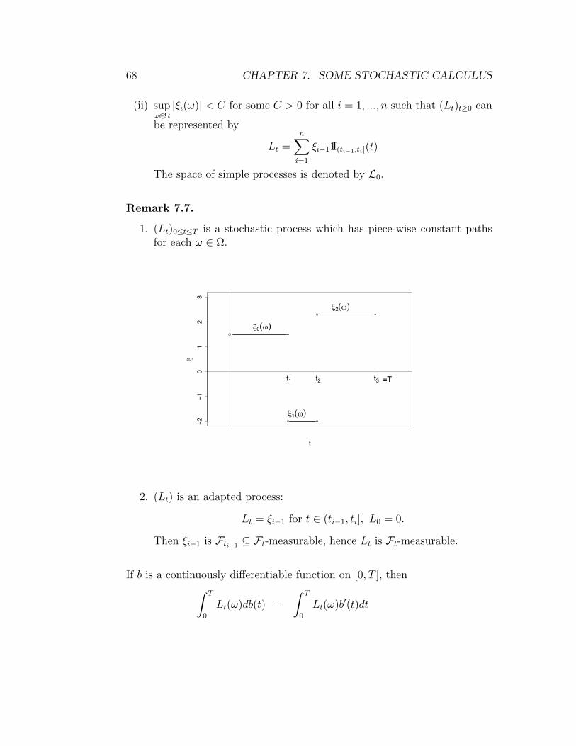
Remark 7.7.

1. (Lt)0≤t≤T is a stochastic process which has piece-wise constant pathsfor each ω ∈ Ω.

21

01

23

t

0( )

1( )

2( )

t1 t2 t3 =T

2. (Lt) is an adapted process:

Lt = ξi−1 for t ∈ (ti−1, ti], L0 = 0.

Then ξi−1 is Fti−1⊆ Ft-measurable, hence Lt is Ft-measurable.

If b is a continuously differentiable function on [0, T ], then∫ T

0

Lt(ω)db(t) =

∫ T

0

Lt(ω)b′(t)dt


=n∑i=1

∫ ti

ti−1

ξi−1(ω)b′(t)dt

=n∑i=1

ξi−1(ω)(b(ti)− b(ti−1)).

This relation is the motivation for the definition of∫ T

0LtdWt (but (Wt(ω) is

not differentiable!).

Definition 7.8 (Ito integral on L0).The Ito integral for L = (Lt)t≥0 ∈ L0 is defined by

It(L) :=k−1∑i=1

ξi−1(Wti −Wti−1) + ξk(Wt −Wtk),

if tk−1 < t ≤ tk and Lt =n∑i=1

ξi−11I(ti−1,ti](t). This can also be written as

It(L) =n∑i=1

ξi−1(Wti∧t −Wti−1∧t), t ∈ [0, T ],

where a ∧ b := mina, b.

Notation:

It(L) =

∫ t

0

LsdWs

Proposition 7.9 (Properties of It(L), L ∈ L0).

(a) Ito isometry:

E(IT (L))2 = E∫ T

0

L2tdt.

(b) (It(L))t≥0 is square integrable and a continuous martingale.

(c) It(αL+ βK) = αIt(L) + βIt(K) for all L,K ∈ L0 and α, β ∈ R.

Proof:


(a) By a direct computation,

E(IT (L))2 = E

(n∑i=1

ξi−1(Wti −Wti−1)

)2

=n∑i=1

n∑k=1

E(ξi−1ξk−1(Wti −Wti−1

)(Wtk −Wtk−1)

)=

n∑i=1

Eξ2i−1(ti − ti−1) + 0,

because if i 6= k, for example i < k, then by using the tower propertyand taking out what is known

Eξi−1ξk−1(Wti −Wti−1)(Wtk −Wtk−1

)

= EE[ξi−1ξk−1(Wti −Wti−1

)(Wtn −Wtn−1)|Ftk−1

]= Eξi−1ξk−1(Wti −Wti−1

)E[Wtk −Wtk−1

|Ftk−1

]= 0,

since Wtk −Wtk−1is independent from Ftk−1

and E(Wtk −Wtk−1) = 0.

If i = k, then

Eξ2i−1(Wti −Wti−1

)2 = EE[ξ2i−1(Wti −Wti−1

)2|Fti−1

]= Eξ2

i−1E[(Wti −Wti−1

)2|Fti−1

]= Eξ2

i−1(ti − ti−1). (7.1)

On the other hand,

E∫ T

0

L2tdt = E

∫ T

0

(n∑i=1

ξi−11I(ti−1,ti](t)

)2

dt

= E∫ T

0

(n∑i=1

ξ2i−11I(ti−1,ti](t)

)dt

= En∑i=1

ξ2i−1

∫ T

0

1I(ti−1,ti](t)dt

= En∑i=1

ξ2i−1(ti − ti−1). (7.2)

Comparing (7.1) and (7.2) implies the claim (a).


(b) From (a) the square integrability of (It(L))t≥0 follows, because

E(It(L))2 = E∫ t

0

L2sds = E

n∑i=1

ξ2i−1(ti ∧ t− ti−1 ∧ t) ≤ c2t, (7.3)

because ξ2i−1 ≤ c2 by the definition of simple processes. A martingale is

said to be continuous if it has almost surely continuous paths. Hence,it needs to be verified that

P(ω ∈ Ω : (It(L))t≤0 (ω) is continuous in t) = 1.

By the definition of the Brownian motion, t 7→ Wt(ω) is a continuousfunction for all ω ∈ Ω. This implies

It(L)(ω) =n∑i=1

ξi−1(ω)(Wti∧t(ω)−Wti−1∧t(ω))

→n∑i=1

ξi−1(ω)(Wti∧s(ω)−Wti−1∧s(ω)) = Is(L)(ω),

as t→ s and thus It(L)(ω) is continuous in t for all ω ∈ Ω.

Yet it needs to be shown that (It(L))t≥0 is a martingale:

(1) If t ∈ (tk−1, tk], then

It(L) =k−1∑i=1

ξi−1(Wti −Wti−1) + ξk−1(Wt −Wtk−1).

The random variables ξi−1 are Fti−1-measurable, ξk−1 is Ftk−1

-measurable, the terms (Wti −Wti−1

) are Fti-measurable and theterm (Wt −Wtk−1

) is Ft-measurable. Since Fti−1⊆ Ft, It(L) is

Ft-measurable, and (It(L))t≥0 is adapted.

(2) E|It(L)| ≤ (E|It(L)|2)12 <∞, because inequality (7.3).

(3) For 0 ≤ s < t, assume tk−1 < s < t ≤ tk. Then

E[It(L)|Fs] =k−1∑i=1

E[ξi−1(Wti −Wti−1

)|Fs]

+ E[ξk−1(Wt −Wtk−1

)|Fs]


=k−1∑i=1

ξi−1(Wti −Wti−1) + ξk−1(Ws −Wtk−1

)

= Is(L) almost surely.

(c) Clear from the definition.

4 Ito’s integral for general integrands

Is it possible to defineT∫

0

WtdWt ?

The process (Wt) is not piecewise constant, so (Wt) /∈ L0. In this section,the definition of It(L) will be extended to a larger class of integrands L. Theresults are not proven here, but the proofs can be found in [3], [4] and [7].

Definition 7.10. Let L2 be the space of the processes L = (Lt)t∈[0,T ] suchthat

1. L is B([0, T ])⊗F -measurable,

2. L is (Ft)t∈[0,T ]-adapted,

3. ET∫0

L2tdt <∞.

Lemma 7.11. Let L ∈ L2. Then there exists a sequence (Ln)n≥0 of simpleprocesses such that

limn→∞

E∫ T

0

|Lt − Lnt |2dt = 0.

Definition 7.12. Let L ∈ L2. Then define

It(L) := limn→∞

∫ t

0

LnsdWs,

where the limit is in L2-sense, i.e. It(L) is the random variable such that

limn→∞

E(It(L)− It(Ln))2 = 0.

5. ITO’S FORMULA 73

Notation:

It(L) :=

∫ t

0

LsdWs.

Proposition 7.13 (Properties of∫ t

0LsdWs, L ∈ L2).

(a) Ito isometry: E(It(L))2 = E∫ t

0L2sds

(b) (It(L))t≥0 is square integrable and a martingale.

(c) It(αL+ βK) = αIt(L) + βIt(K) almost surely for all α, β ∈ R, L,K ∈L2.

(d) EIt(L) = 0.

Remark 7.14. By (b), (It(L))t≥0 is square integrable and a martingale.What about the continuity of t 7→ It(L)(ω)? So far, for each t ∈ [0, T ] therandom variable It(L) has been defined as a limit in L2-sense, i.e. It(L) isP-a.s. unique.The stochastic processes (Xt)t≥0 and (Yt)t≥0 are called modifications of eachother, if Xt = Yt almost surely for all t ≥ 0. It can be shown that (It(L))t≥0

has a modification which has almost surely continuous paths t 7→ It(L)(ω).From now on we will assume that (It(L))t≥0 refers to the modification whichhas almost surely continuous paths. It can be shown that

limn,m→∞

E sup0≤t≤T

∣∣∣∣ ∫ t

0

Lns − Lms dWs

∣∣∣∣2 = 0.

5 Ito’s formula

Assume a given stochastic process

Xt = X0 +

∫ t

0

b(s)ds+

∫ t

0

σ(s)dWs,

where the second term is a Riemann-integral with

• b(s) = b(s, ω) is jointly measurable, i.e. b is B([0, T ])⊗F -measurable,

• b(s) is Fs-measurable, E∫ T

0|b(s)|ds <∞, and


• σ ∈ L2.

Then the Ito integral is defined.

Proposition 7.15 (Ito’s formula). Let f ∈ C1,2([0, T ] × R). Then for t ∈[0, T ]

f(t,Xt) = f(0, X0) +

∫ t

0

∂f

∂t(s,Xs)ds

+

∫ t

0

∂f

∂x(s,Xs)(b(s)ds+ σ(s)dWs) +

1

2

∫ t

0

∂2f

∂x2(s,Xs)σ

2(s)ds.

Remark 7.16. If (∂f

∂x(s,Xs)σ(s)

)s∈[0,T ]

/∈ L2,

then a more general definition is needed for∫ t

0

∂f

∂x(s,Xs)σ(s)dWs.

(see, for example [3], section 3.1.)

Example 7.17. Let f(t, x) = ex−t2 , Xt = Wt. Then

f(t,Wt) = eWt− t2 = 1 +

∫ t

0

−1

2eWs− s2ds+

∫ t

0

eWs− s2dWs +1

2

∫ t

0

eWs− s2ds

= 1 +

∫ t

0

eWs− s2dWs.

8. Continuous time marketmodels

1 The stock price process

A continuous time market model consists of

(1) a complete probability space (Ω,F ,P),

(2) a filtration F = (Ft)0≤t≤T , that

• satisfies the ’usual conditions’

• F0 is trivial, i.e. for A ∈ F0, P(A) = 0 or P(A) = 1.

• FT = F .

(3) d+ 1 traded assets:

• d stocks: S1(t), ..., Sd(t)

• one bank account S0(t)

Now assume, that r : [0, T ] → [0,∞) with r(0) = 0, for example r(t) = r0t,r0 ≥ 0, and S0(t) = er(t). We can interpret the stocks model as a ’generalizedgeometric Brownian motion’. For d = 1 let

S1(t) = S1(0) exp

(∫ t

0

σ(s)dWs +

∫ t

0

(α(s)− 1

2σ2(s)

)ds

), (8.1)

where α, σ are bounded, measurable and adapted processes. Now Ito’s for-mula implies that

(S1(t)) is given by (8.1) ⇐⇒ S1(t) = S1(0) +

∫ t

0

α(s)S1(s)ds+

∫ t

0

σ(s)S1(s)dWs

75

76 CHAPTER 8. CONTINUOUS TIME MARKET MODELS

for all t ∈ [0, T ].

Special case: geometric Brownian motion (with drift)

S1(t) = S1(0)eσWt+(α−σ2

2)t, t ∈ [0, T ]

⇐⇒ S1(t) = S1(0) + α

∫ t

0

S1(s)ds+ σ

∫ t

0

S1(s)dWs, t ∈ [0, T ]

For d > 1, the random influence is assumed to come from a d-dimensionalBrownian motion

W = (W 1t , ...W

dt )t∈[0,T ],

where (W 1t )t∈[0,T ], (W

2t )t∈[0,T ], ..., (W

dt )t∈[0,T ] are independent Brownian mo-

tions. Then for i = 1, ..., d, Si(t) is defined as

Si(t) := Si(0) +

∫ t

0

αi(s)Si(s)ds+d∑j=1

∫ t

0

Si(s)σij(s)dWjs (8.2)

for all t ∈ [0, T ], αi, σij bounded, measurable and adapted.

2 Trading strategies

Assume, that there are shares/stocks S1(t), ..., Sd(t), t ∈ [0, T ] of the form8.2, and a non-random bank account S0(t), t ∈ [0, T ].

Definition 8.1. The stochastic processes

ϕ(t) := (ϕ0(t), ..., ϕd(t)), t ∈ [0, T ],

form a trading strategy, if

(a) the ϕi : [0, T ]×Ω→ R are B([0, T ])⊗F -measurable and adapted (ϕi(t)is Ft-measurable for all t), i = 0, ..., d.

(b)d∑i=0

T∫0

Eϕi(t)2Si(t)2dt <∞.

In the definition above, ϕi(t) denotes the amount of shares of asset i (1 ≤i ≤ d) held in the portfolio at time t. ϕi(t) < 0 means short sales: sellinga stock which is not owned, only borrowed.

9. Risk neutral pricing

We want to have a method to compute the fair price of an option (so thatriskless profit = arbitrage is not possible). The method will be ’risk neutralpricing’ using an equivalent martingale measure.

Definition 9.1. A probability measure Q defined on (Ω,F) is a (strong)equivalent martingale measure if

(i) Q is equivalent to P, i.e. Q(A) = 0 ⇐⇒ P(A) = 0 for all A ∈ F

(ii) The discounted price processes

S :=

(S(t)

S0(t)

)t≥0

are a Q-martingales.

It will be shown that (like in the discrete time case) for certain models anequivalent martingale measure (EMM) exists

• uniquely

• not uniquely (there are more than one EMM) or

• not at all.

Definition 9.2.

(a) The value of the portfolio ϕt = (ϕ0(t), ϕ1(t), ..., ϕd(t)) at time t isgiven by

Vt(ϕ) :=d∑i=0

ϕi(t)Si(t), t ∈ [0, T ].

The process (Vt(ϕ))t∈[0,T ] is called the value process of the tradingstrategy ϕ.

77

78 CHAPTER 9. RISK NEUTRAL PRICING

(b) The gains process is

Gt(ϕ) :=d∑i=0

∫ t

0

ϕi(u)dSi(u),

if the stochastic integral is well-defined.

(c) A trading strategy is called self-financing if

Vϕ(t) = Vϕ(0) +Gϕ(t), t ∈ [0, T ].

Remark 9.3. If

Si(t) = Si(0) +

t∫0

αi(s)Si(s)ds+d∑j=1

∫ t

0

Si(s)σij(s)dWjs ,

then we define∫ t

0

ϕi(u)dSi(u) :=

∫ t

0

ϕi(u)αi(u)Si(u)du+d∑j=1

∫ t

0

ϕi(u)Si(u)σijdWju .

By denoting the first term by A and the second term by B, then by Holder’sinequality

E(∫ t

0

ϕi(u)dSi(u)

)2

= E(A+B)2 ≤ 2EA2 + 2EB2.

We can easily see that the gains process is square integrable:

EA2 = E(∫ t

0

ϕi(u)αi(u)Si(u)du

)2

≤ tE∫ t

0

(ϕi(u)Si(u)αi(u)

)2

du <∞

and for EB2,

E(∫ t

0

ϕi(u)Si(u)σij(u)dW ju

)2

=d∑j=1

E∫ t

0

(ϕi(u)Si(u)σij(u)

)2

du <∞.

The above is true, because

E∫ t

0

a(u)dW 1u

∫ t

0

b(u)dW 2u = 0

if W 1 and W 2 are independent Brownian motions, and a, b ∈ L2. See theexercises for (a(u)) and (b(u)) simple processes.

79

Definition 9.4. Assume Q is an equivalent martingale measure. A strategyϕ is admissible, if

(i) ϕ is self-financing,

(ii) Vt(ϕ) ≥ 0, t ∈ [0, T ]

(iii) EQ sup0≤t≤T

Vt(ϕ)2 <∞, where

Vt(ϕ) :=Vt(ϕ)

S0(t).

Definition 9.5. A trading strategy ϕ is called an arbitrage opportunityif

(i) ϕ is admissible,

(ii) V0(ϕ) = 0 and P(VT (ϕ) > 0) > 0.

Any non-negative random variable H we will call an option. Often H isa function of Si(T ), the terminal value of the i-th share price process. Forexample,

H = f(Si(T )) = (Si(T )−K)+,

the European call option. But there also exist ”basket options” like

H =(S1(T ) + ...+ Sd(T )−K

)+

or ”Asian options”, depending on the whole process S, for example,

H =

(1

T

∫ T

0

S1(t)dt−K)+

.

Proposition 9.6. If the equivalent martingale measure Q exists uniquelyand EQH

2 <∞, then there exists an admissible trading strategy

ϕ =(ϕ0(s), ..., ϕd(s)

)s∈[0,T ]

such that

H = V0(ϕ) +d∑i=1

∫ T

0

ϕi(s)dSi(s).

80 CHAPTER 9. RISK NEUTRAL PRICING

The theorem says that if there is exactly one Q ∼ P such that (Si(t))t∈[0,T ],i = 1, ..., d are Q-martingales, then any option H ≥ 0 with EQH

2 < ∞ can

be hedged. It can be shown, that EQ∫ T

0ϕi(t)dSi(t) = 0. Hence

EQH = V0(ϕ),

which is the fair price of the option H.

Since arbitrage opportunities appear in reality only temporarily, the aim isto construct market models which do not admit arbitrage opportunities.

Theorem 9.7 (Fundamental Theorem of Asset pricing). If a market modelhas an equivalent martingale measure Q, then it does not admit arbitrage.

Remark 9.8. The other implication is not always true in this general setting.But there exists an ”if and only if”-relation, if ”no arbitrage opportunities”is replaced by ”no free lunch with vanishing risk” (see [2], page 235).

10. The Black-Scholes model

Assume a filtered probability space (Ω,F ,P,F) and a Brownian motion Wwith respect to F. We will consider the model suggested by Black and Scholes.The model consists of

• one riskless asset S0(t) = ert, t ≥ 0, where r > 0 is the (instantaneous)interest rate, and

• one risky asset S(t) = s0eσWt−σ

2

2t+µt.

It can be easily checked, that S0(t) solves the differential equationdS0(t) = rS0(t)dtS0(0) = 1,

(10.1)

and that S0(t) is the only solution of (10.1). It is also true, thatdS(t) = σS(t)dWt + µS(t)dtS(0) = s0

(10.2)

is solved by

S(t) = s0eσWt−σ

2

2t+µt.

1 The equivalent martingale measure QWe want to determine the equivalent martingale measure Q. It has theproperties:

1. Q ∼ P

2. S(t) = S(t)S0(t)

= s0eσWt−σ

2

2t+(µ−r)t, t ∈ [0, T ] is a Q-martingale.

81

82 CHAPTER 10. THE BLACK-SCHOLES MODEL

The measure Q can be found using Girsanov’s theorem:

Proposition 10.1 (Girsanov’s theorem).

Let (θt)t∈[0,T ] be an adapted process satisfying∫ T

0θ2sds <∞ almost surely and

such that the process

Ht = exp

(−∫ t

0

θsdWs −1

2

∫ t

0

θ2sds

), t ∈ [0, T ]

is a martingale. Then with respect to Q,

Q(A) :=

∫A

HTdP(ω),

the process

Bt := Wt +

∫ t

0

θsds, 0 ≤ t ≤ T

is a standard Brownian motion.

Remark 10.2. It is often difficult in applications to check whether (Ht)t isa martingale. The Novikov condition

Ee12

∫ T0 θ2t dt <∞

is a sufficient condition for (Ht) being a martingale.Now by Ito’s formula,

S(t) = s0 + σ

∫ t

0

S(s)dWs +

∫ t

0

S(s)(−σ2

2+ (µ− r))ds

+σ2

2

∫ t

0

S(s)ds

= s0 + σ

∫ t

0

S(s)dWs +

∫ t

0

S(s)(µ− r)ds

= s0 + σ

∫ t

0

S(s)dBs,

with Bs = Ws + µ−rσs. Hence Q is given by Q(A) :=

∫AHtdP, where

Ht := exp

(−µ− r

σWt +

(µ− r)2

2σ2t

).

2. PRICING: THE BLACK-SCHOLES FORMULA 83

2 Pricing: The Black-Scholes formula

Assume we have an European call-option with strike price K > 0 at timeT > 0,

f(x) = (x−K)+

What is the fair price of the option f(ST ) = (ST −K)+? This question willbe answered using the so-called martingale representation (see [7]).

Definition 10.3. Let (Xt)0≤t≤T be a stochastic process on a complete prob-ability space (Ω,F ,P).

(i) Set

Ft := σ(Xs, 0 ≤ s ≤ t)

= the smallest σ-algebra, such that Xs is

Ft-measurable for all s ∈ [0, t].

Then (Ft)t∈[0,T ] is the filtration generated by (Xt).

(ii) Now all P-null sets of F are added to each Ft:

FXt := σ(Ft ∪ A ∈ F : P(A) = 0).

Then (FXt )t∈[0,T ] is again a filtration, and it is called the augmentednatural filtration of (Xt)t∈[0,T ].

Proposition 10.4 (Brownian martingale representation).Let (Ω,F ,P) be a complete probability space and (Wt)t∈[0,T ] a Brownian mo-tion, (FWt )t∈[0,T ] its augmented natural filtration. Let (Mt)t∈[0,T ] be a martin-gale with respect to (FWt )t∈[0,T ] such that EM2

T < ∞. Then there exists an

(FWt )t∈[0,T ]-adapted process (Lt)t∈[0,T ], such that E∫ T

0L2tdt <∞, and

Mt = M0 +

∫ t

0

LsdWs almost surely for all t ∈ [0, T ].

The above Proposition 10.4 is applied in the following way:


• ( ˜S(T )−K)+ is square integrable:

EQ(( ˜S(T )−K)+)2 ≤ EQ(S(T ))2 = 1 <∞

• Mt := EQ[ ˜(S(T )−K)+|FBt

]is a square integrable martingale with re-

spect to (FBt )t∈[0,T ], where (Bs)s∈[0,T ] is a Brownian motion with respectto Q.

• Proposition 10.4 implies that there exists a process (Ls)s∈[0,T ] which is

(FBt )-adapted and EQ∫ T

0L2sds <∞, such that

˜(S(T )−K

)+= MT = M0 +

∫ T

0

LsdBs. (10.3)

On the other hand, if the equation

˜(S(T )−K

)+= VT (ϕ) = V0(ϕ) +

∫ T

0

ϕ(u)dS(u) (10.4)

would be true with (ϕ(u)) being adapted and EQ( ∫ T

0ϕ(u)dS(u)

)2<∞, then

(ϕ(u))u∈[0,T ] would be a self-financing trading strategy. Because of

S(t) = s0 + σ

∫ t

0

S(s)dBs,

where (Bs)s∈[0,T ] is the Brownian motion with respect to Q, (10.4) implies

( ˜S(T )−K)+ = V0(ϕ) +

∫ T

0

ϕ(u)S(u)σdBu. (10.5)

By comparing (10.3) and (10.5),

0 = EQ

∣∣∣∣( ˜S(T )−K)+ − ( ˜S(T )−K)+

∣∣∣∣2= EQ

(M0 +

∫ T

0

LsdBs − V0(ϕ)−∫ T

0

ϕ(u)S(u)σdBu

)2

= EQ

(M0 − V0(ϕ)

)2

2. PRICING: THE BLACK-SCHOLES FORMULA 85

+ 2EQ

(M0 − V0(ϕ)

)(∫ T

0

LsdBs −∫ T

0

ϕ(u)S(u)σdBu

)+ EQ

(∫ T

0

LsdBs −∫ T

0

ϕ(u)S(u)σdBu

)2

= EQ

(M0 − V0(ϕ)

)2

+ EQ

∫ T

0

∣∣∣Lu − ϕ(u)S(u)σ∣∣∣2 du,

where the last equality follows from the fact that EQ∫ T

0Lu−ϕ(u)S(u)σdBu =

0 and Ito ’s isometry. This implies, that

V0(ϕ) = M0

ϕ(u) =Lu

S(u)σand

Vt(ϕ) = Mt

Q⊗ dt-almost everywhere. Since (Bu) is a Brownian motion with respect toQ, by Proposition 7.13

Vt(ϕ) = V0(ϕ) +

∫ t

0

ϕ(u)S(u)σdBu, t ∈ [0, T ]

is a square integrable martingale.Now, if

V0(ϕ) = the price of the option at time 0.

Vt(ϕ) = discounted price of the option at time t.

Then the price is

Vt(ϕ) = ertEQ

[(S(T )−K)+

erT

∣∣∣∣FBt ]= EQ[e−r(T−t)(S(T )−K)+|FBt ]

= EQ

[e−r(T−t)

(S(t)

S(T )

S(t)−K

)+ ∣∣∣∣FBt]

= EQ

[e−r(T−t)

(xS(T )

S(t)−K

)+ ∣∣∣∣FBt] ∣∣∣∣∣

x=S(t)

,


where S(t) is independent from FBt and FBt -measurable. For the last equality,see [6], proposition A.25.Now, set

F (t, x) := EQe−r(T−t)

(xS(T )

S(t)−K

)+

,

then Vt(ϕ) = F (t, S(t)). By S(u) = s0eσBu−σ

2u2

F (t, x) = EQe−r(T−t)

(xerT S(T )

ertS(t)−K

)+

= e−r(T−t)EQ

(xer(T−t)eσ(BT−Bt)−σ

2(T−t)2 −K

)+

= e−r(T−t)EQ

(xer(T−t)eσ(BT−t)−σ

2(T−t)2 −K

)+

,

since BT − Btd= BT−t. By substituting T − t =: a and denoting X = BT−t√

T−t ,

making X standard Gaussian, i.e. P(X ≤ z) = N0,1(z), F (t, x) can beexpressed as

F (t, x) = e−raEQ

(xeraeσ

√aX−σ

2a2 −K

)+

= e−ra1√2π

∫ ∞−∞

(xeraeσ

√az−σ

2a2 −K

)+

e−z2

2 dz

=1√2π

∫ ∞−∞

(xeσ

√az−σ

2a2 −Ke−ra

)1Iz+d2≥0e

− z2

2 dz,

where

d1 =log x

K+ (r + σ2

2)a

σ√a

and d2 = d1 − σ√a,

with a = T − t. Then z + d2 ≥ 0 = −z ≤ d2, and

F (t, x) =1√2π

∫ d2

−∞

(xe−σ

√az−σ

2a2 −Ke−ra

)e−

z2

2 dz

= ... = xN0,1(d1)−Ke−raN0,1(d2).

This is the Black-Scholes formula

F (t, x) = xN0,1(d1)−Ke−r(T−t)N0,1(d2).

3. EXAMPLE OF INFINITELY MANY EMM’S 87

3 Example of infinitely many EMM’s

Assume that (Ω,F ,P) is a complete probability space and (W 1t ) and (W 2

t )

are independent F−Brownian motions. Let (St)t∈[0,T ], St := eσWt−σ2t2 be the

share price process. Then (St) is a P-martingale with respect to (FW 1

t )t∈[0,T ],

the natural filtration of (W 1t ). Set Ht := eθW

2t −

Tθ2

2 , θ > 0. Then

Qθ(A) := EP (1IAHT )

is an equivalent martingale measure for any θ > 0 :

• 0 < HT <∞ P-a.s.

• Since HTStSs

and FW1s are independent, as are HT and St

Ss, and HT and

ST are square integrable, the martingale property is satisfied as

EQθ [St|FW1s ] = E

[HTSt|FW1

s

]= SsE

[HT

StSs

∣∣∣∣FW1s

]= SsE

(HT

StSs

)= SsEHTE

StSs

= Ss,

because EHT = 1 = EStSs

.

4 Example of no EMM’s

Assume r = 0 and price processes are chosen as

Si(t) = Si(0)eWt+(µi− 12

)t, i = 1, 2 and µ1 6= µ2.

Then H1i = e−µiWT+

µ2i2T defines according to Proposition 10.1 the equivalent

martingale measure Qi for Si. For Q1 = Q2 the condition µ1 = µ2 would beneeded.

11. Bonds

A bond is a debt security. The issuer (government, credit institutes, com-panies) has to pay interest (coupon) once or twice a year and to repay theamount (principal) and the interest at the maturity time. Zero-coupon bondsdo not pay interest until maturity time. Modeling of a zero-coupon bond:

• p(t, T ) = price of a zero-coupon bond at time t ≤ T that pays 1 e attime T .

• p(t, t) = 1.

If the ’instantaneous’ interest rate is a constant r, then

p(t, T ) = e−r(T−t)

because for 1 e one would get er(T−t) interest for the time amount T − t.(The relation between annual interest rate ra and instantaneous interest rater is

ra = limn→∞

(1 +

rT

n

)n− 1 = erT − 1 for T = 1 year. )

Now we assume that the interest rate is not fixed, but changes randomly.

Similar to Proposition 9.7, it holds that if the market model (Ω,F ,P,F, S)has an equivalent martingale measure, then it does not admit arbitrage.If Q is an equivalent martingale measure, then Q ∼ P and the discountedprice processes of the basic securities have to be Q-martingales. If weconsider the bond market, then the discounted zero-coupon bonds have tobe Q-martingales.

Definition 11.1. The fair price for a zero-coupon bond with maturityT at time t is

p(t, T )

S0(t):= EQ

[1

S0(T )

∣∣∣∣Ft] almost surely,

89

90 CHAPTER 11. BONDS

under the assumption S0(t) = exp(∫ t

0r(s)ds) with a random adapted process

(r(s))s∈[0,T ]. So p(t, T ), the price of a bond at time t which matures at T is

p(t, T ) = EQ

[e−

∫ Tt r(s)ds|Ft

].

Remark 11.2. There are other approaches to describe bonds and bondprices. See [2] for the Heath-Jarrow-Morton-model.The ”short rate” r(s) can be modeled by several processes:Vasicek model, see [3]:

r(s) = r0 +

∫ s

0

α− βr(u)du+

∫ s

0

γdWu,

Cox-Ingersoll-Ross, see [3]:

r(s) = r0 +

∫ s

0

α− βr(u)du+

∫ s

0

σ(u)√r(u)dWu,

and other more complicated ones.

12. Currency markets

Sometimes assets are needed in several countries simultaneously. We con-sider two countries: a domestic country with interest rate rd and a foreigncountry with interest rate rf , and bank accounts in both countries, denotedby Bd(t) = erdt and Bf (t) = erf t. We introduce an exchange rate process(Q(t))t≥0 to pass denomination in foreign to domestic currency. (Q(t))t≥0 de-pends on the two economies, the policies of the governments, etc, so (Q(t)) isinfluenced by a ’multidimensional noise’, modelled with independent Brow-nian motions (W 1

t )t, ..., (Wdt )t. Then

dQ(t) = Q(t)µdt+Q(t)(σ1dW1t + ...+ σddW

dt )

Q(0) = q0 > 0

if and only if

Q(t) = q0 exp

(d∑i=1

σiWit +

(µ− 1

2

d∑i=1

σ2i

)t

), (12.1)

where µ and σi, i = 1, ...d are positive constants. We compute the discountedvalue of the foreign savings account (discounted by the domestic interest rate)in domestic currency,

Q(t) :=Bf (t)Q(t)

Bd(t), (12.2)

and get from (12.1) and (12.2) that

Q(t) = q0 exp

(d∑i=1

σiWit +

(µ− 1

2

d∑i=1

σ2i

)t+ (rf − rd)t

).

91

92 CHAPTER 12. CURRENCY MARKETS

To avoid arbitrage between domestic and foreign bond markets, such anequivalent martingale measure Q(t) is needed that

Q(t) = q0 +

∫ t

0

Q(s)(µ+ rf − rd)ds+d∑i=1

σi

∫ t

0

Q(s)dW is

does not have the drift term∫ t

0Q(s)(µ + rf − rd)ds. In case there exist d

independent trading assets the equivalent martingale measure Q is unique.It is called the domestic martingale measure. By considering currencyoptions, for example the currency European call-option:

f(Q(t)) := (Q(T )−K)+

Then the fair price at time t is given by

C(t) = EQ[e−rd(T−t)(Q(T )−K)+|Ft].

13. Credit risk

Credit risk is the risk of loss if a loan or its interest is not paid back. Thereexists two methods to model credit risk:

• reduced form modelsThe modeler has the same information as the market. A point processis used to describe the default event.

• structural modelsThe modeler has the same information as the firms manager. Thetraded assets itself are used to describe the default event.

Default event is the event where the debtor does not make a scheduledpayment - ’the debtor defaults’.

1 A simple model for credit risk

Let (Ω,F ,P,F) be a filtered probability space, and T ∗ > 0 a time horizon.We assume a firm’s value process

V (t) = V (0) + r

∫ t

0

V (s)ds− δ∫ t

0

V (s)ds+ σ

∫ t

0

V (s)dWs,

where r is the interest rate and δ is either the constant dividend rate if δ > 0or the constant ’pay-in’ rate, if δ < 0. The process can be equivalentlywritten (see page 82) as

V (t) = V (0) exp

(σWt −

σ2t

2+ (r − δ)t

).

We assume that there exists an equivalent martingale measure Q to have anarbitrage-free market. Then the discounted tradable securities which pay no

93

94 CHAPTER 13. CREDIT RISK

dividends follow Q-martingales. By assuming that the firm’s value processis a tradable security, we get for σ ≥ 0 that

V (t) := V (0)eσWt−σ2t2 = e−(r−δ)tV (t)

is a Q-martingale if (Wt) is a Q-Brownian motion. Now we consider a zero-coupon bond with notational amount F (=face value) and maturity T ≤ T ∗.So the cash received by the ’owner of the defaultable claim’ (= the one whogives the credit to the firm in form of buying the bond) is

DT =

F, if VT ≥ FVT , if VT < F.

Now, define a ’default time’

τ := T1IVT<F +∞1IVT≥F.

Then the payoff for the ’equity owners’ (=owners of the firm) is

CT = (VT − F )+,

which can be interpreted as a call option on the value of the firm. ByBlack-Scholes formula (see page 86),

Ct = EQ(VT − F )+ = Vte−δ(T−t)N0,1(d1)− Fe−r(T−t)N0,1(d2) (13.1)

with

d1 =log Vt

F+ (r − δ + σ2

2)(T − t)

σ√T − t

= d2 + σ√T − t.

The bond owners’ (= the one who gave the credit) payoff is

DT = F − (F − VT )+.

What is the fair price of this bond, or in other words, how much creditcan this firm get?

Proposition 13.1. Assume the above assumptions. Then

Bonds = a risk-free payment− put-option on the value of the firm,

so we have

p(t, T ) = Fe−r(T−t) − EQ[e−r(T−t)(F − VT )+

∣∣FT ]= Vte

−δ(T−t)N0,1(−d1) + Fe−r(T−t)N0,1(d2).

1. A SIMPLE MODEL FOR CREDIT RISK 95

ProofThe proof is done by using the call-put-parity

CT − PT = (VT − F )+ − (F − VT )+ = VT − F

and knowing thate−(r−δ)tVt = Mt

is a martingale. We have

Ct = ertEQ[CT∣∣Ft]

andPt = ertEQ

[PT∣∣Ft],

which imply that

Ct − Pt = e−r(T−t)EQ[VT∣∣Ft]− e−r(T−t)F

= e−r(T−t)+(r−δ)T−(r−δ)tVt − e−r(T−t)F= Vte

−δ(T−t) − e−r(T−t)F.

This yieldsFe−r(T−t) − Pt = Vte

−σ(T−t) − CtThis implies

p(t, T ) = e−r(T−t)EQ[DT |Ft

]= e−r(T−t)EQ

[F − PT |Ft

]= Fe−r(T−t) − Pt= Vte

−δ(T−t) − Vte−δ(T−t)N0,1(d1) + Fe−r(T−t)N0,1(d2)

= Vte−δ(T−t)N0,1(−d1) + Fe−r(T−t)N0,1(d2)

96 CHAPTER 13. CREDIT RISK

Bibliography

[1] E. Benhamou Global Derivatives: Products, Theory and Practice. WorldScientific, 2007

[2] N.H Bingham and R. Kiesel Risk-Neutral Vauluation: Pricing and Hedgingof Financial Derivatives.

[3] S. Geiss Stochastic Processes in continuous time.www.math.jyu.fi/∼geiss/scripts/stochastic-sde.pdf

[4] C. Geiss and S. Geiss An introduction to probability theory.www.math.jyu.fi/∼geiss/scripts/introduction-probability.pdf

[5] R. Elliott, P. Kopp Mathematics of Financial Markets. Springer, 2000

[6] D. Lamberton and B. Lapeyre Stochastic Calculus Applied to Finance.Chapman & Hall, 1996.

[7] I. Karatzas and S. Shreve Brownian motion and Stochastic Calculus

[8] M. Steele Stochastic Calculus and Financial Applications

97

financial mathematics - jyväskylän...

Documents