Long run economic growth, part 2. The Solow growth model

Macroeconomics II Joanna Siwińska-Gorzelak

WNE UW

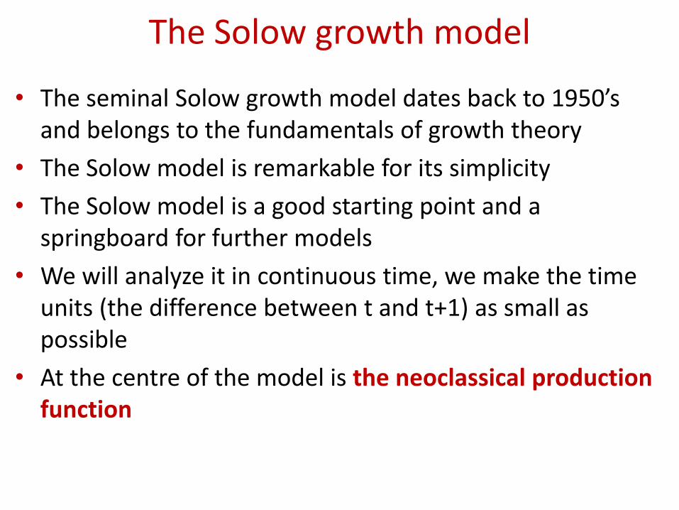
The Solow growth model

• The seminal Solow growth model dates back to 1950’s and belongs to the fundamentals of growth theory

• The Solow model is remarkable for its simplicity

• The Solow model is a good starting point and a springboard for further models

• We will analyze it in continuous time, we make the time units (the difference between t and t+1) as small as possible

• At the centre of the model is the neoclassical production function

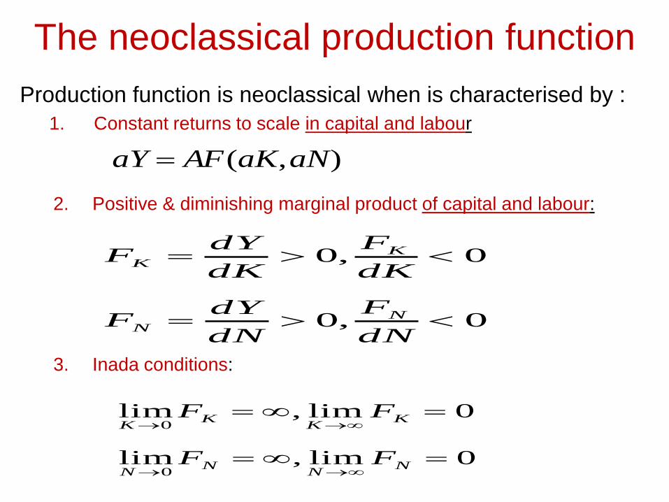
The neoclassical production function

Production function is neoclassical when is characterised by :

1. Constant returns to scale in capital and labour

2. Positive & diminishing marginal product of capital and labour:

3. Inada conditions:

),( aNaKAFaY

0,0

0,0

dN

F

dN

dYF

dK

F

dK

dYF

NN

KK

0lim,lim

0lim,lim

0

0

NN

NN

KK

KK

FF

FF

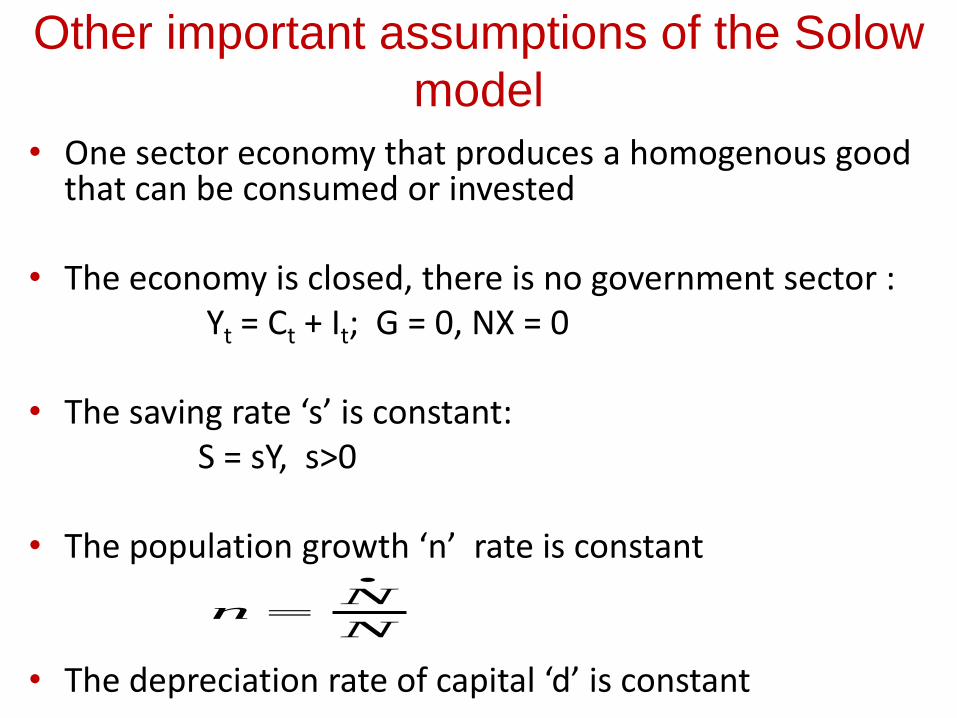
Other important assumptions of the Solow

model

• One sector economy that produces a homogenous good that can be consumed or invested

• The economy is closed, there is no government sector : Yt = Ct + It; G = 0, NX = 0

• The saving rate ‘s’ is constant: S = sY, s>0

• The population growth ‘n’ rate is constant

• The depreciation rate of capital ‘d’ is constant

N

Nn

A temporary assumption (just for now)

• To make our analysis easier, we will assume that

technology is constant and equal to 1

• We will change this assumption very soon

• For now, the (neoclassical) production function is:

Y=A F (K, N) = F (K, N)

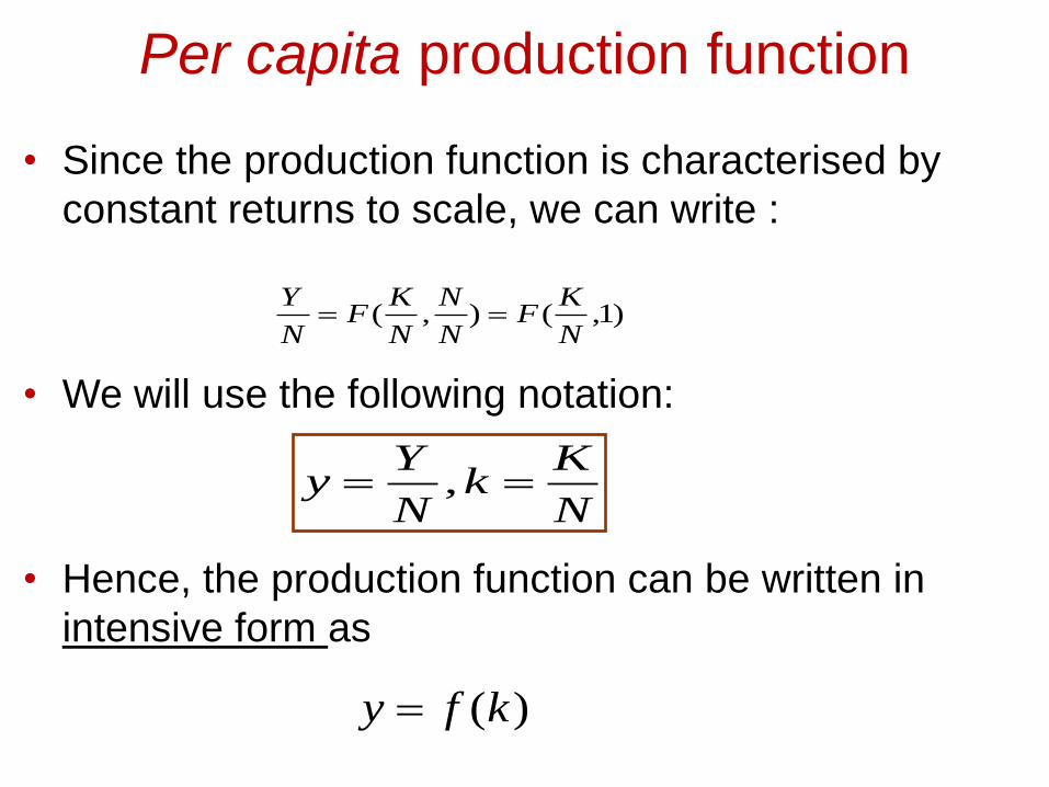
Per capita production function

• Since the production function is characterised by

constant returns to scale, we can write :

• We will use the following notation:

• Hence, the production function can be written in

intensive form as

)1,(),(N

KF

N

N

N

KF

N

Y

N

Kk

N

Yy ,

)(kfy

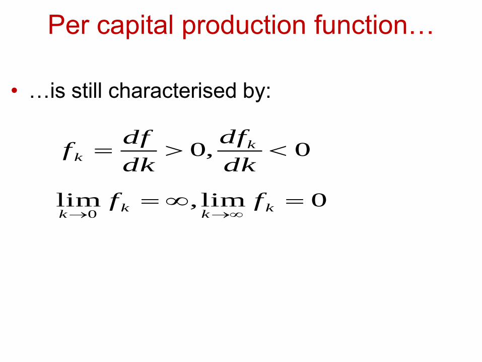
Per capital production function…

• …is still characterised by:

0lim,lim

0,0

0

k

kk

k

kk

ff

dk

df

dk

dff

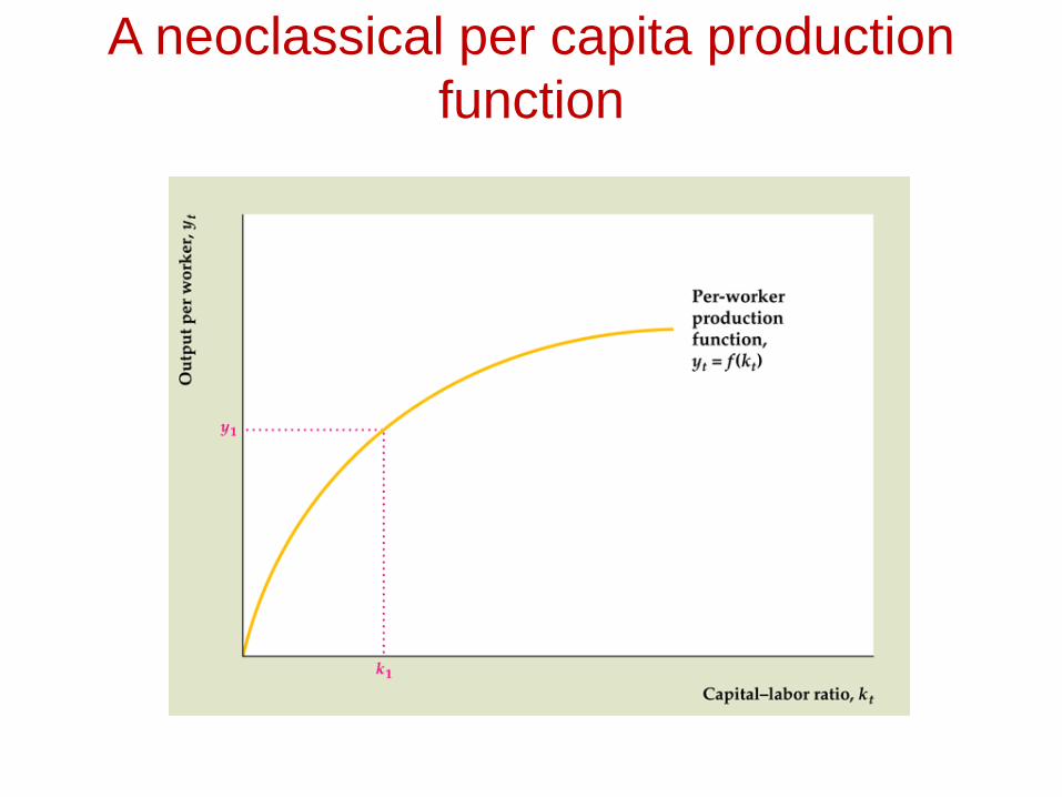
A neoclassical per capita production

function

Notice that

• The per capita production function depends only on

per capita capital stock

• If we understand the dynamics of capital per capita

we can understand economic growth!

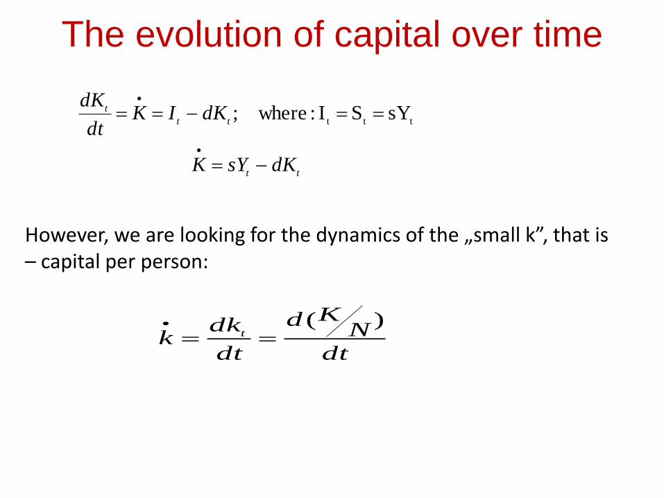
The evolution of capital over time

tt

tt

t

dKsYK

dKIKdt

dK

tttsYSI:where;

However, we are looking for the dynamics of the „small k”, that is – capital per person:

dt

NKd

dt

dkk t

)(

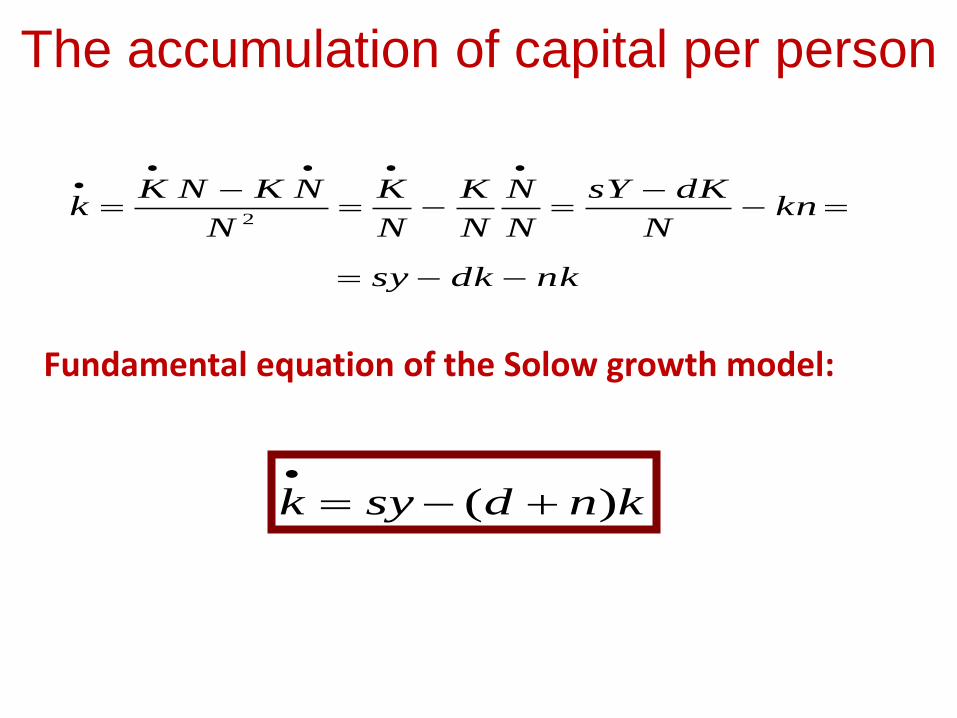
The accumulation of capital per person

nkdksy

knN

dKsY

N

N

N

K

N

K

N

NKNKk

2

Fundamental equation of the Solow growth model:

kndsyk )(

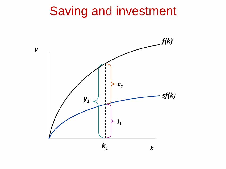
Saving and investment

y

k

f(k)

sf(k)

k1

y1

i1

c1

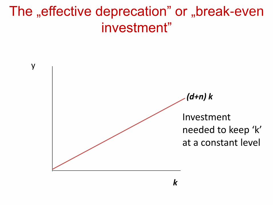
The „effective deprecation” or „break-even

investment”

y

k

(d+n) k

Investment needed to keep ‘k’ at a constant level

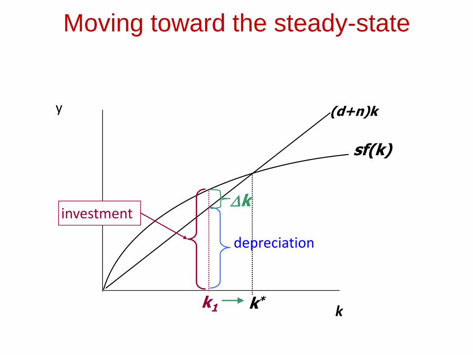
Moving toward the steady-state

y

k

sf(k)

(d+n)k

k* k1

investment

depreciation

k

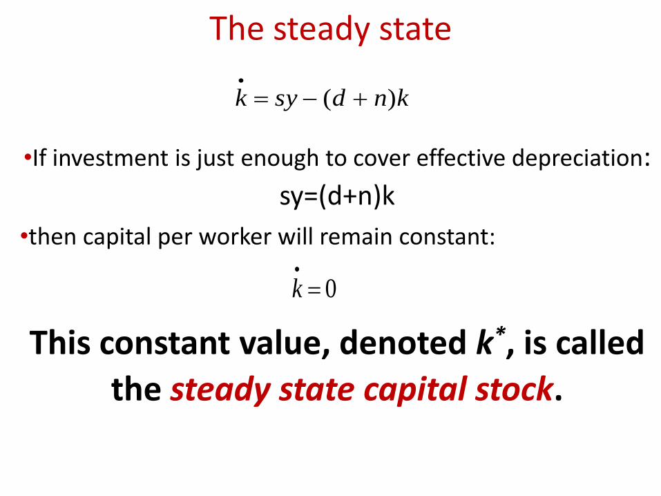
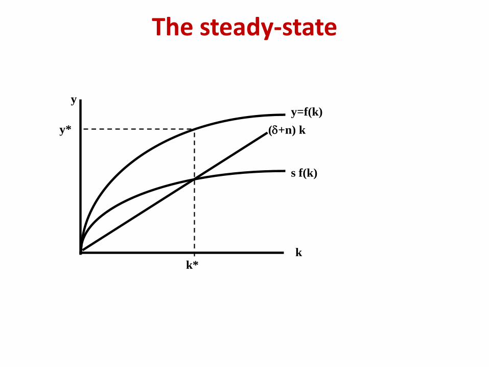
The steady state

•If investment is just enough to cover effective depreciation:

sy=(d+n)k

•then capital per worker will remain constant:

This constant value, denoted k*, is called

the steady state capital stock.

kndsyk )(

0

k

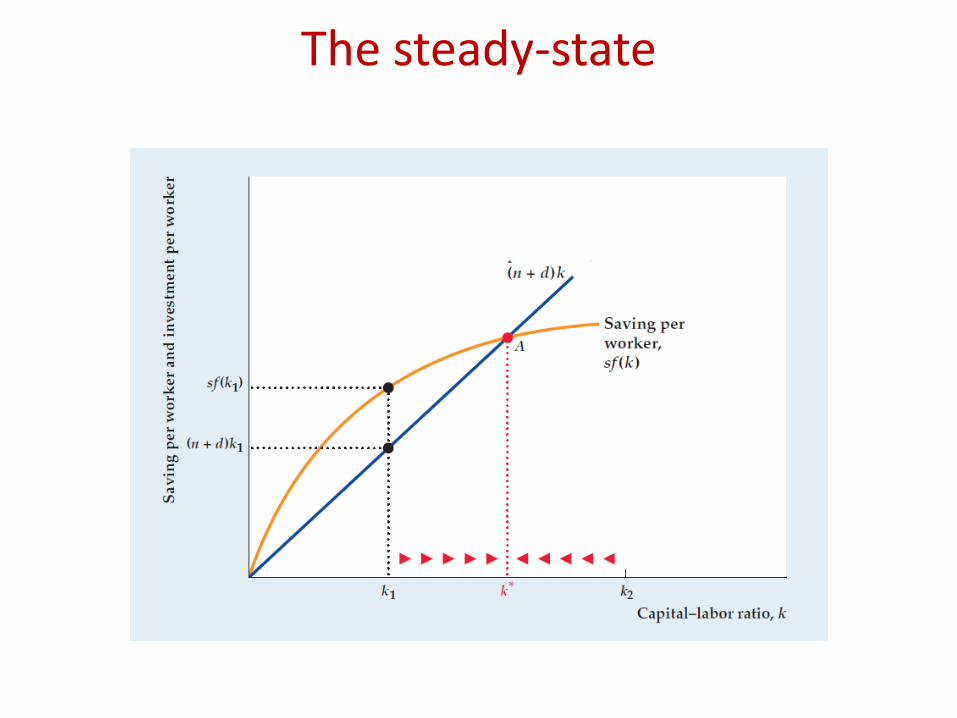
The steady-state

The steady-state

y

k

y*

y=f(k)

s f(k)

k*

(+n) k

The steady-state

• The only possible steady-state capital–labor ratio is k*

• Output at that point is y* = f(k*); consumption is c* = f(k*) – (n + d)k*

• If k begins at some level other than k*, it will move toward k*

– For k below k*, saving > the amount of investment needed to keep k constant, so k rises

– For k above k*, saving < the amount of investment needed to keep k constant, so k falls

The steady-state

• We have established that in the steady-state, capital per person is constant.

• That, of course implies that output per person and consumption per person are also constant:

0

cyk

The Solow’s suprise

• Investment in new capital cannot lead to continued growth in per capita income.

• What can lead to sustained growth of output per person?

• As we will see next week – technology!

The steady-state

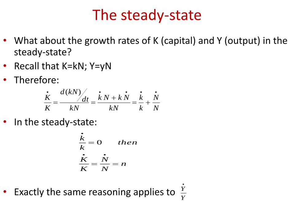
• What about the growth rates of K (capital) and Y (output) in the steady-state?

• Recall that K=kN; Y=yN

• Therefore:

• In the steady-state:

• Exactly the same reasoning applies to

N

N

k

k

kN

NkNk

kN

dtkNd

K

K

)(

nN

N

K

K

thenk

k

0

Y

Y

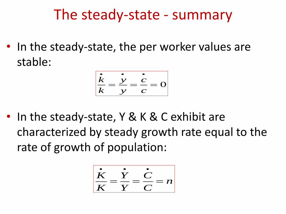
The steady-state - summary

• In the steady-state, the per worker values are stable:

• In the steady-state, Y & K & C exhibit are characterized by steady growth rate equal to the rate of growth of population:

0

c

c

y

y

k

k

nC

C

Y

Y

K

K

Steady-state: a Cobb-Douglas production function

• Assume a Cobb-Douglas function:

• Intensive form (per worker):

• The steady-state:

1NKY

ky

1

)(

)(

0)(

0*

knd

s

kndsk

kndskk

k

1

1

)(*

nd

sk

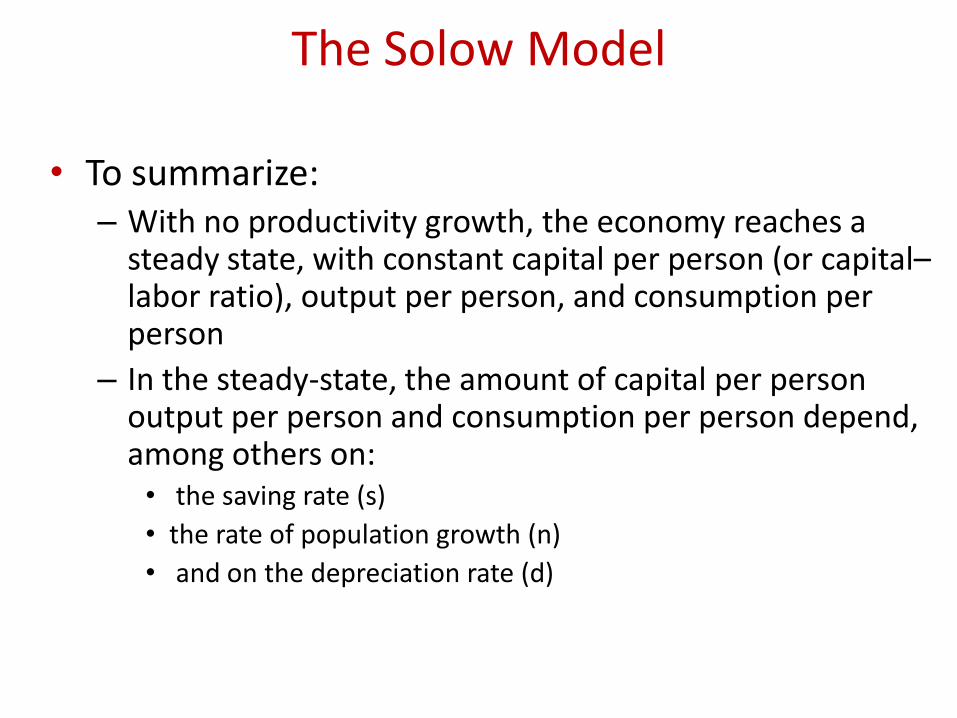
The Solow Model

• To summarize: – With no productivity growth, the economy reaches a

steady state, with constant capital per person (or capital–labor ratio), output per person, and consumption per person

– In the steady-state, the amount of capital per person output per person and consumption per person depend, among others on:

• the saving rate (s)

• the rate of population growth (n)

• and on the depreciation rate (d)

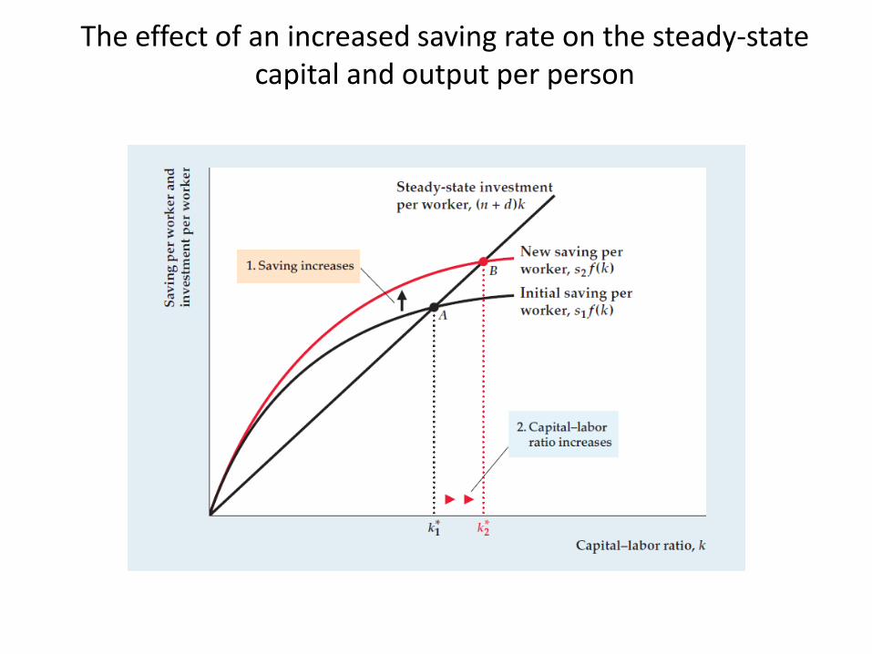
The effect of an increased saving rate on the steady-state capital and output per person

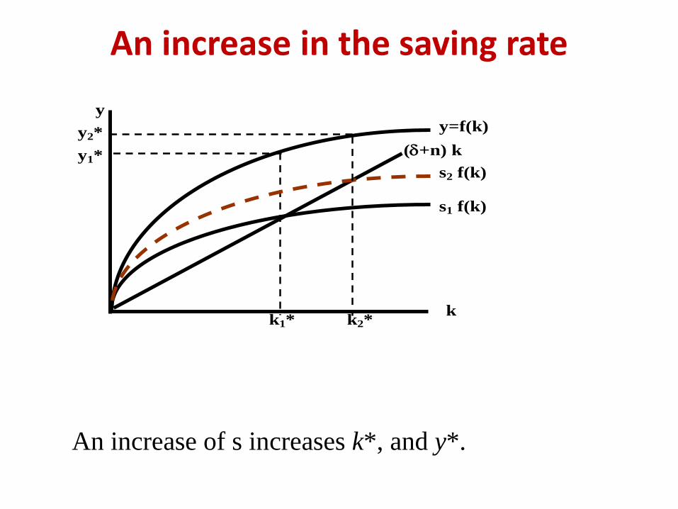
An increase in the saving rate

An increase of s increases k*, and y*.

y

k

y1*

y=f(k)

s1 f(k)

k1*

(+n) k

k2*

y2*

s2 f(k)

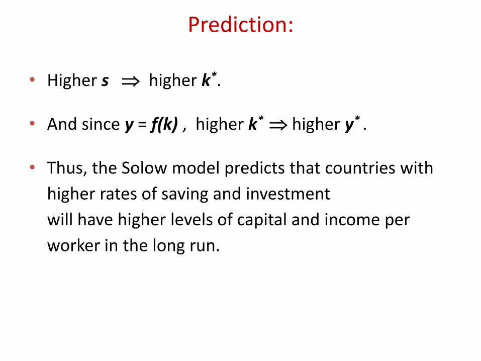
Prediction:

• Higher s higher k*.

• And since y = f(k) , higher k* higher y* .

• Thus, the Solow model predicts that countries with

higher rates of saving and investment

will have higher levels of capital and income per

worker in the long run.

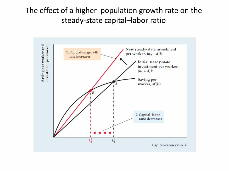
The effect of a higher population growth rate on the steady-state capital–labor ratio

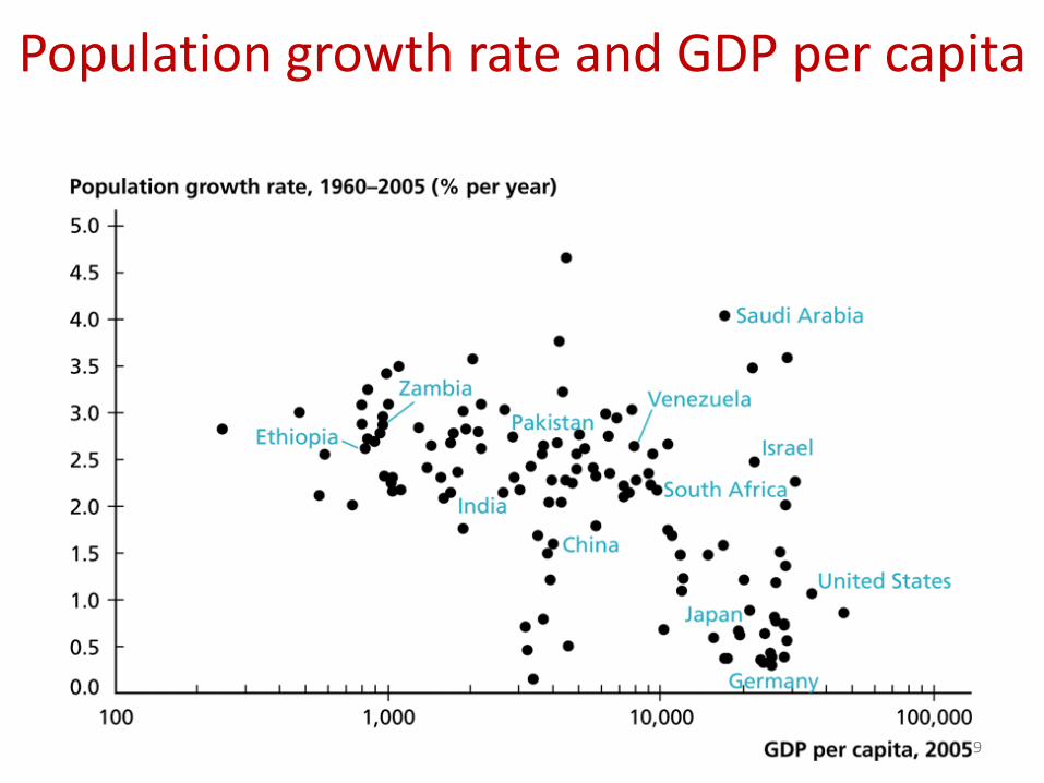
Population growth rate and GDP per capita

29

The Solow Model

• Should a policy goal be to reduce population growth? – Doing so will raise consumption per worker – Note however that the Solow model also assumes that

the proportion of the population of working age is fixed (exactly: population = workers)

• But when population growth changes, this may change the % of the working-age population

• Changes in cohort sizes may cause problems for social security systems and areas like health care

The Golden Rule: Introduction

• Different values of s lead to different steady states. How do we know which is the “best” steady state?

• The “best” steady state has the highest possible consumption per person: c* = (1–s) f(k*).

• An increase in s

– leads to higher k* and y*, which raises c*

– reduces consumption’s share of income (1–s), which lowers c*.

• So, how do we find the s and k* that maximize c* (in the steady-state)?

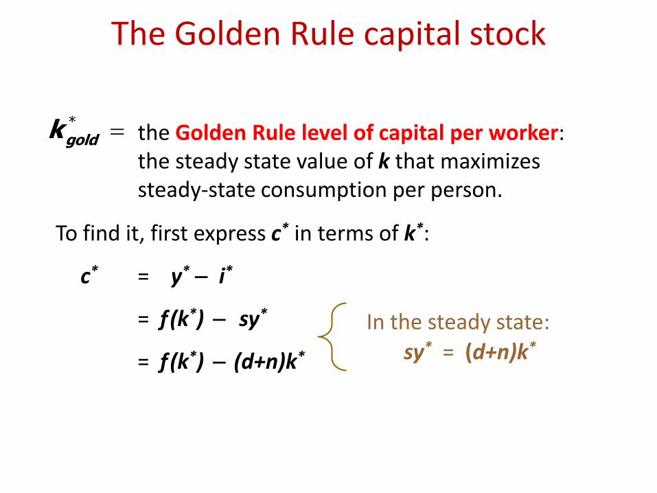
The Golden Rule capital stock

the Golden Rule level of capital per worker: the steady state value of k that maximizes steady-state consumption per person.

*

goldk

To find it, first express c* in terms of k*:

c* = y* i*

= f (k*) sy*

= f (k*) (d+n)k*

In the steady state:

sy* = (d+n)k*

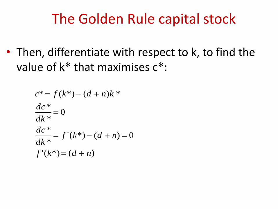
• Then, differentiate with respect to k, to find the value of k* that maximises c*:

The Golden Rule capital stock

)(*)('

0)(*)('*

*

0*

*

*)(*)(*

ndkf

ndkfdk

dc

dk

dc

kndkfc

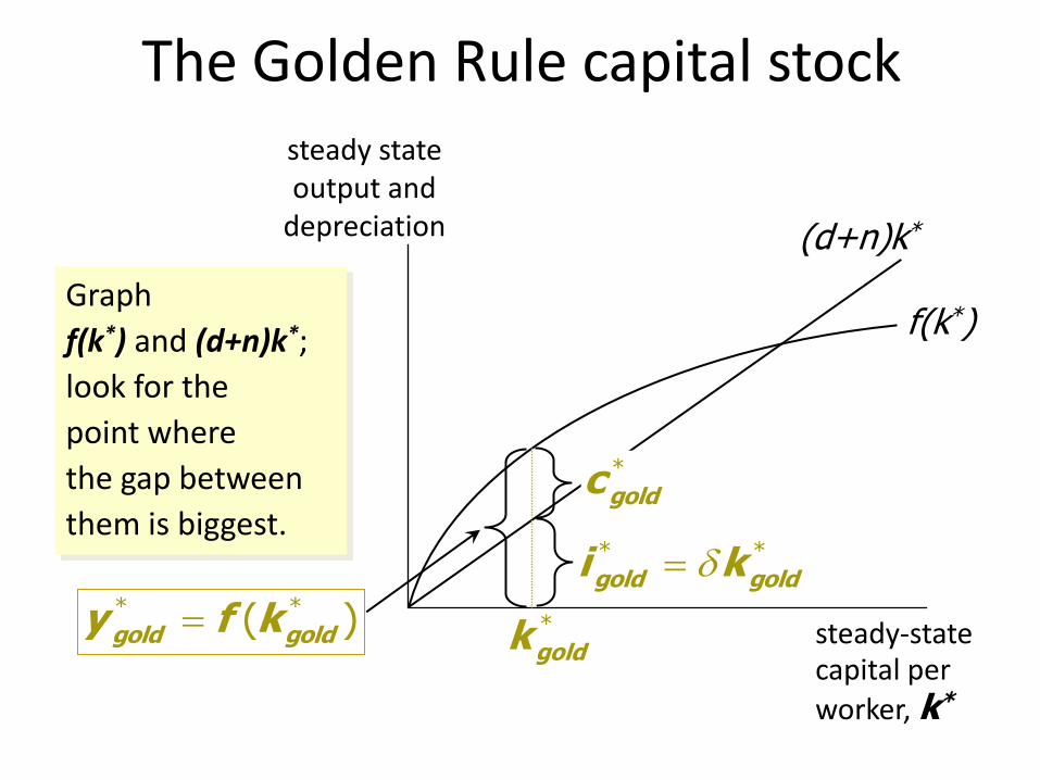
Graph

f(k*) and (d+n)k*;

look for the

point where

the gap between

them is biggest.

The Golden Rule capital stock steady state output and

depreciation

steady-state capital per

worker, k*

f(k*)

(d+n)k*

*

goldk

*

goldc

* *

gold goldi k* *( )gold goldy f k

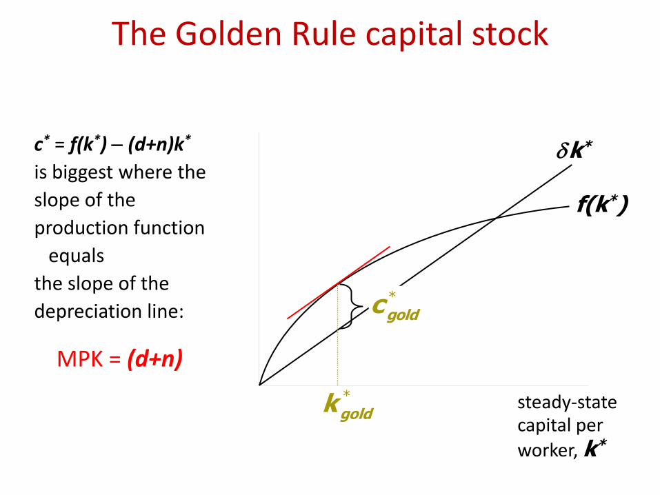
The Golden Rule capital stock

c* = f(k*) (d+n)k*

is biggest where the

slope of the

production function

equals

the slope of the

depreciation line:

steady-state capital per

worker, k*

f(k*)

k*

*

goldk

*

goldc

MPK = (d+n)

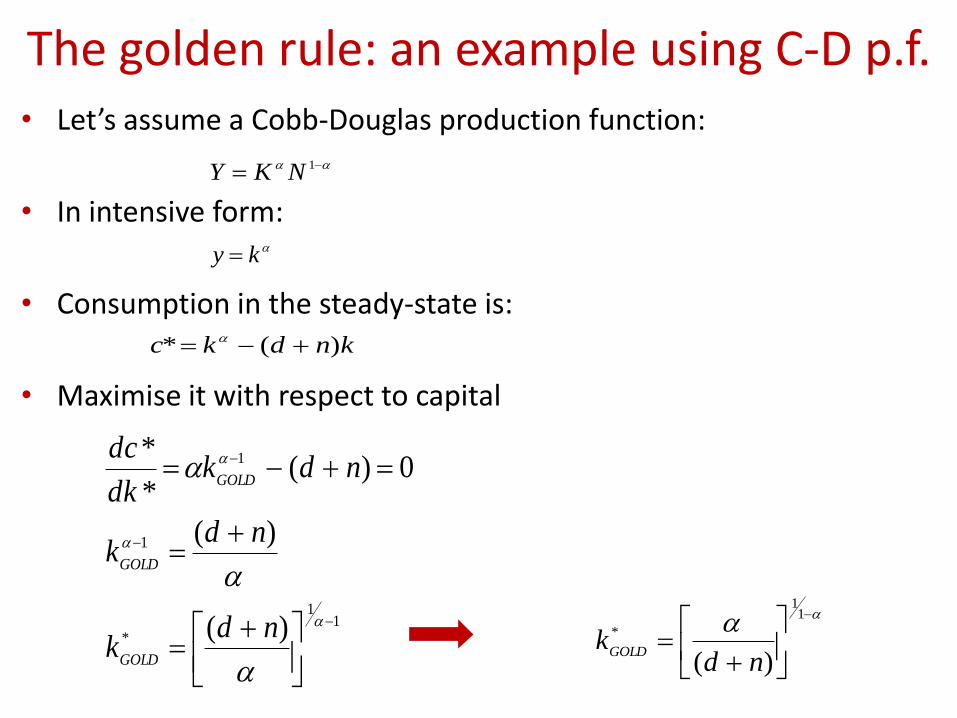
The golden rule: an example using C-D p.f. • Let’s assume a Cobb-Douglas production function:

• In intensive form:

• Consumption in the steady-state is:

• Maximise it with respect to capital

1NKY

ky

kndkc )(*

11

*

1

1

)(

)(

0)(*

*

ndk

ndk

ndkdk

dc

GOLD

GOLD

GOLD

11

*

)( ndk

GOLD

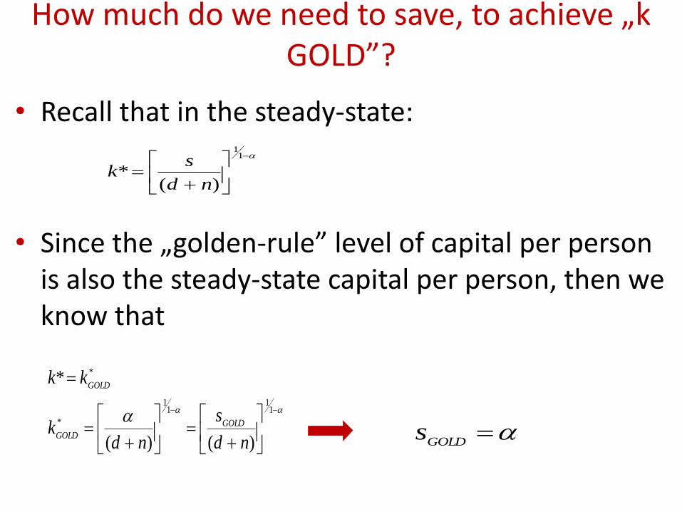
How much do we need to save, to achieve „k GOLD”?

• Recall that in the steady-state:

• Since the „golden-rule” level of capital per person is also the steady-state capital per person, then we know that

11

)(*

nd

sk

11

11

*

*

)()(

*

nd

s

ndk

kk

GOLD

GOLD

GOLD

GOLD

s

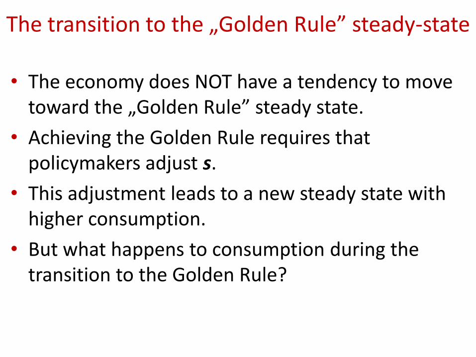
The transition to the „Golden Rule” steady-state

• The economy does NOT have a tendency to move toward the „Golden Rule” steady state.

• Achieving the Golden Rule requires that policymakers adjust s.

• This adjustment leads to a new steady state with higher consumption.

• But what happens to consumption during the transition to the Golden Rule?

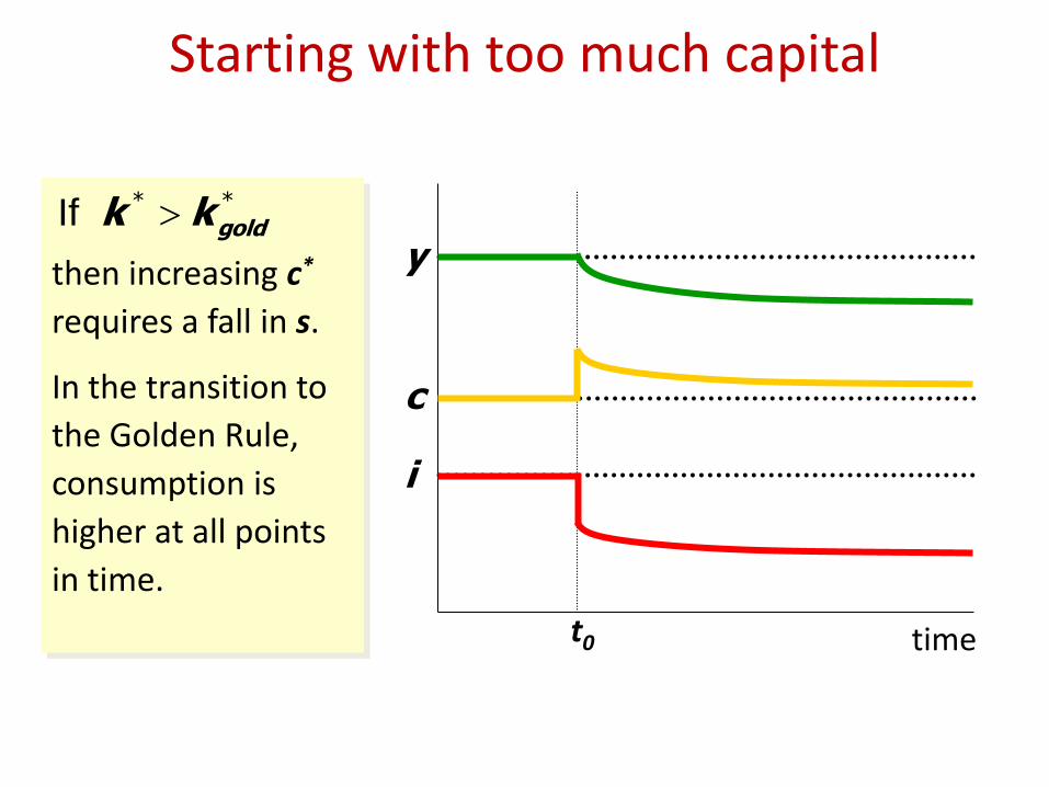
Starting with too much capital

then increasing c*

requires a fall in s.

In the transition to

the Golden Rule,

consumption is

higher at all points

in time.

If goldk k* *

time t0

c

i

y

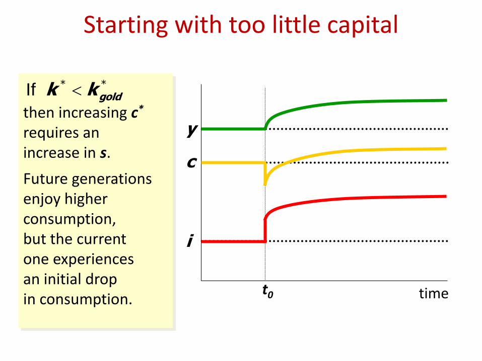
Starting with too little capital

then increasing c* requires an increase in s.

Future generations enjoy higher consumption, but the current one experiences an initial drop in consumption.

If goldk k* *

time t0

c

i

y

Summary

• The economy will reach a steady-state, where the values of capital & output & consumption per worker will be constant

• Investment in new capital (and the growth of population) cannot lead to continued growth in per capita income.

• GDP per worker in the steady-state depends on (among others): the saving rate and the population growth rate

What’s ahead?

• Discussing convergence (next week)

• Adding technology to the Solow’s model (next week)

• A very quick glimse at different growth models (in two weeks)