MACROECONOMICS I

March 7th, 2014

Class 3. Explaining Economic Growth.

The Solow-Swan Model

Homework assignment #1 is now posted on the web

Deadline: March 21st, before the class (12:00)

Submission: One hard copy of answers from a group

N!B! NO late submissions will be accepted

Announcement

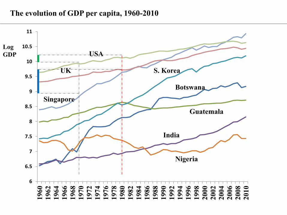
The evolution of GDP per capita, 1960-2010

6

6.5

7

7.5

8

8.5

9

9.5

10

10.5

11

1960

1962

1964

1966

1968

1970

1972

1974

1976

1978

1980

1982

1984

1986

1988

1990

1992

1994

1996

1998

2000

2002

2004

2006

2008

2010

USA

UK

Singapore

Guatemala

S. Korea

India

Nigeria

Botswana

Log

GDP

Solow-Swan Model of Economic Growth(1956)

What drives changes in GDP per capita in the long run?

• Robert Solow (1956)

Economic environment (a set of assumptions)

• A single composite good

• Two factors of production: capital and labor

• Two agents: firms and households

• A closed economy

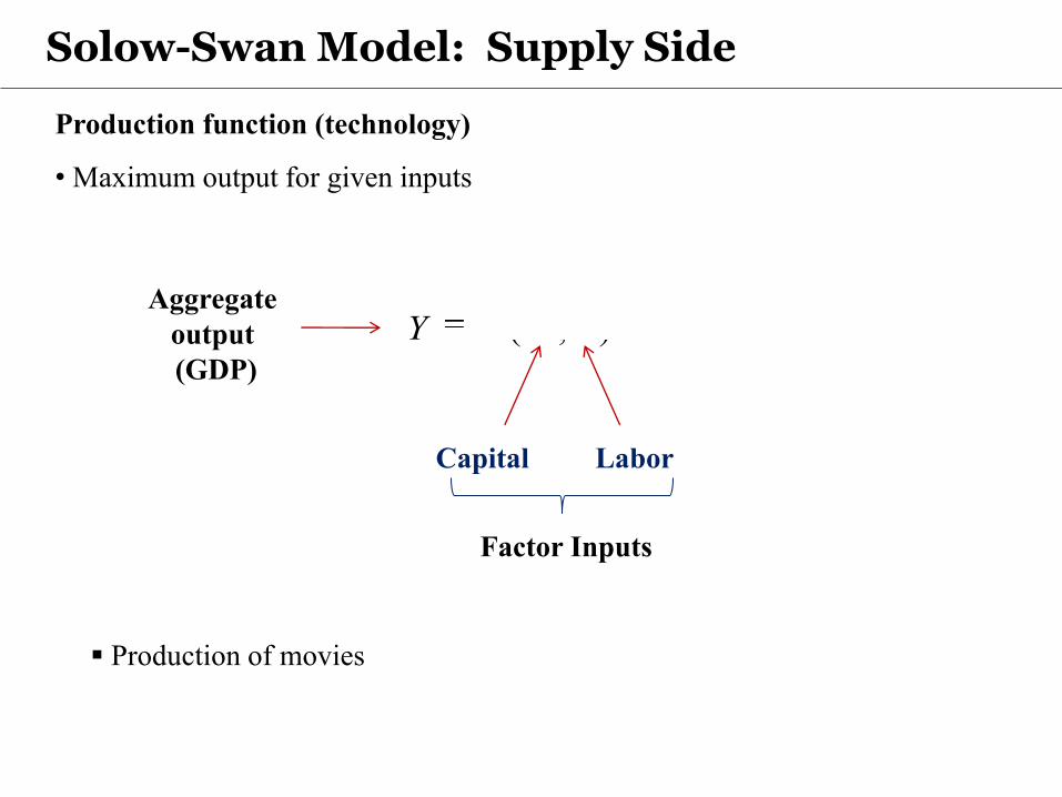
Solow-Swan Model: Supply Side

( , )Y F K L

Production function (technology)

• Maximum output for given inputs

Capital Labor

Factor Inputs

Aggregate

output

(GDP)

Production of movies

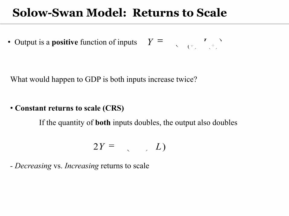
Solow-Swan Model: Returns to Scale

What would happen to GDP is both inputs increase twice?

• Constant returns to scale (CRS)

If the quantity of both inputs doubles, the output also doubles

- Decreasing vs. Increasing returns to scale

2 (2 , 2 )Y F K L

• Output is a positive function of inputs ( ) ( )

( , )Y F K L

Solow-Swan Model: Returns to Factor Inputs

• Diminishing returns to factor inputs

For a fixed L, an increase in K would lead to smaller and smaller increase in Y

For a fixed K, an increase in L would lead to smaller and smaller increase in Y

• Increasing returns to factor inputs

What would happen to GDP if only one input increases?

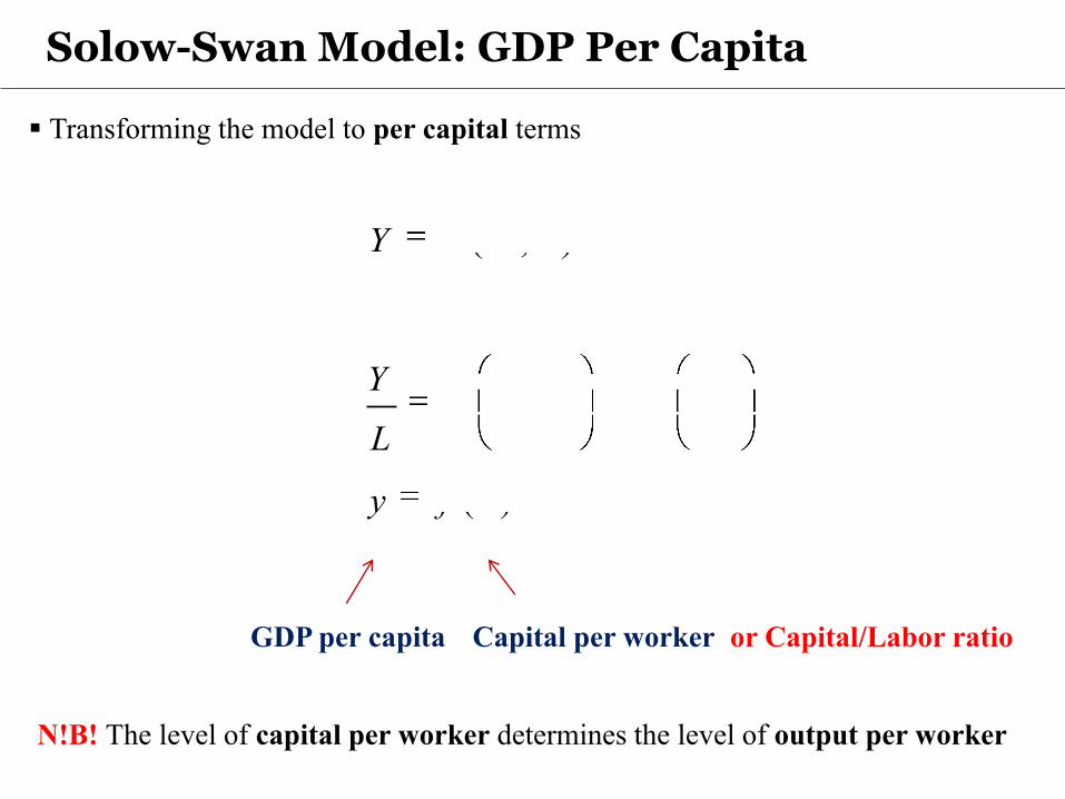
Solow-Swan Model: GDP Per Capita

, 1

( )

Y K KF F

L L L

y f k

GDP per capita Capital per worker

Transforming the model to per capital terms

( , )Y F K L

N!B! The level of capital per worker determines the level of output per worker

or Capital/Labor ratio

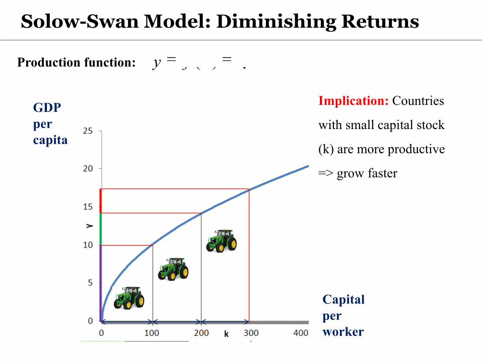
Solow-Swan Model: Diminishing Returns

Production function: ( )y f k k

Implication: Countries

with small capital stock

(k) are more productive

=> grow faster

GDP

per

capita

Capital

per

worker

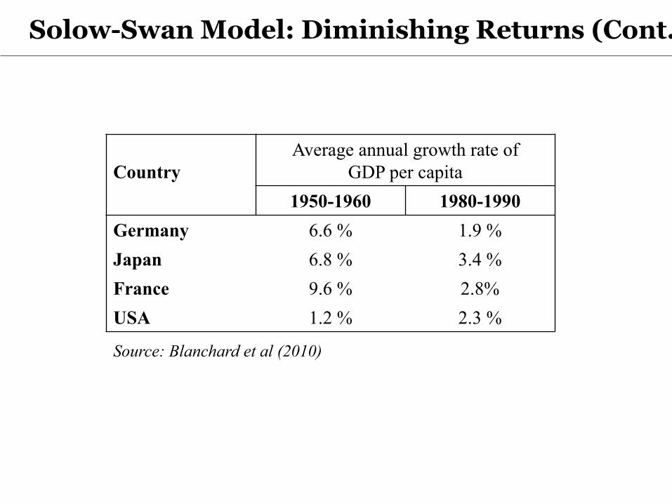
Solow-Swan Model: Diminishing Returns (Cont.)

Country

Average annual growth rate of

GDP per capita

1950-1960 1980-1990

Germany 6.6 % 1.9 %

Japan 6.8 % 3.4 %

France 9.6 % 2.8%

USA 1.2 % 2.3 %

Source: Blanchard et al (2010)

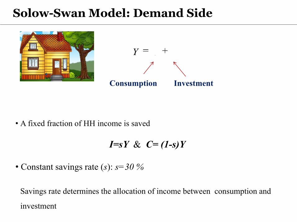
Solow-Swan Model: Demand Side

Y C I

Consumption Investment

• A fixed fraction of HH income is saved

I=sY & C= (1-s)Y

• Constant savings rate (s): s=30 %

Savings rate determines the allocation of income between consumption and

investment

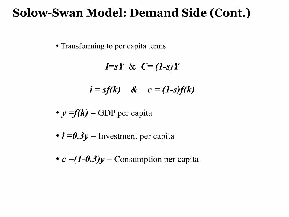
Solow-Swan Model: Demand Side (Cont.)

• Transforming to per capita terms

I=sY & C= (1-s)Y

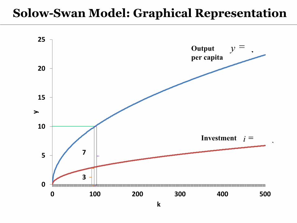
i = sf(k) & c = (1-s)f(k)

• y =f(k) – GDP per capita

• i =0.3y – Investment per capita

• c =(1-0.3)y – Consumption per capita

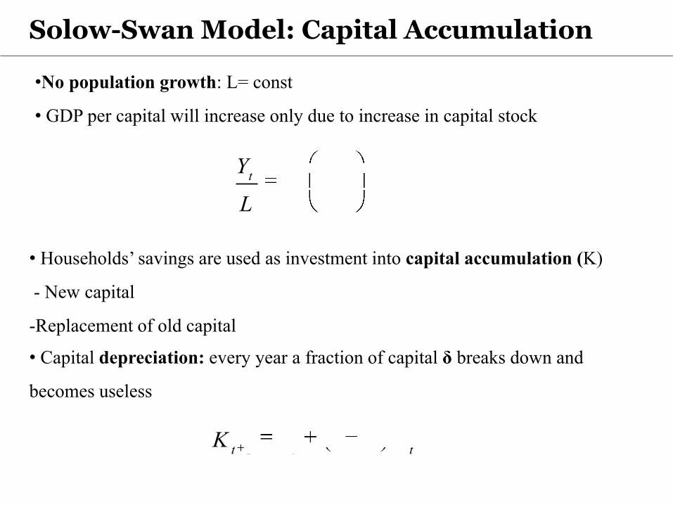
Solow-Swan Model: Capital Accumulation

•No population growth: L= const

• GDP per capital will increase only due to increase in capital stock

• Households’ savings are used as investment into capital accumulation (K)

- New capital

-Replacement of old capital

t tY K

FL L

• Capital depreciation: every year a fraction of capital δ breaks down and

becomes useless

1(1 )

t t tK I K

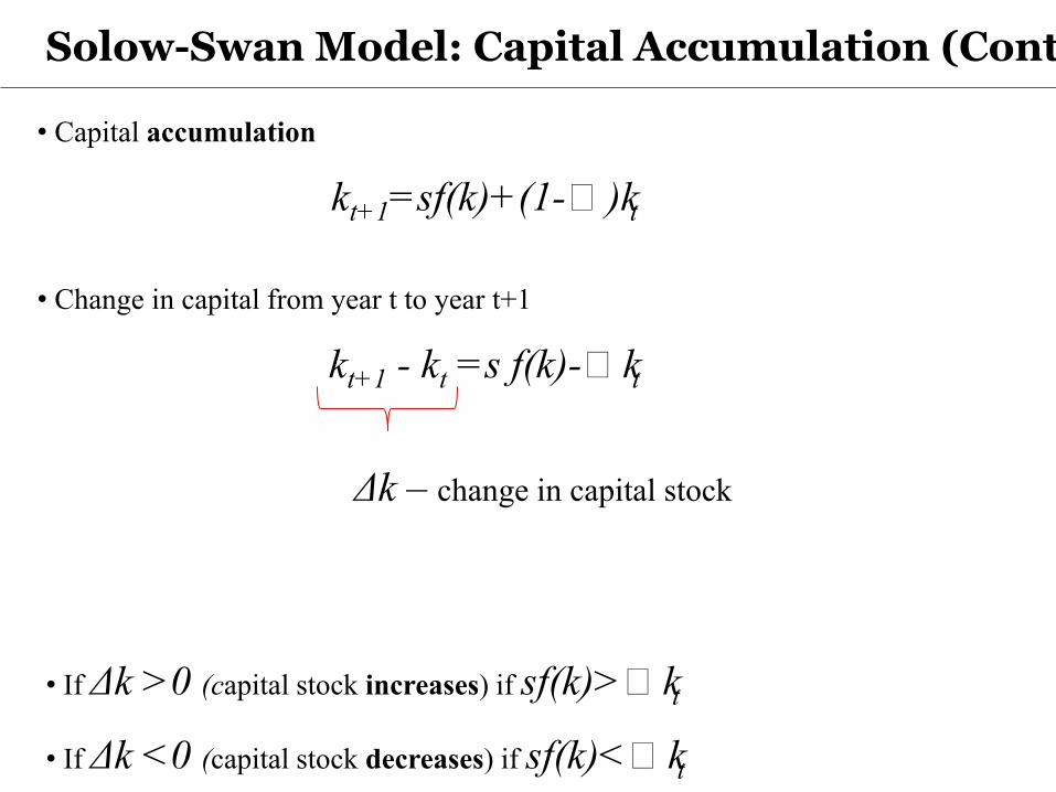
Solow-Swan Model: Capital Accumulation (Cont.)

• Capital accumulation

kt+1=sf(k)+(1-ẟ)kt

• Change in capital from year t to year t+1

kt+1 - kt =s f(k)-ẟkt

Δk – change in capital stock

• If Δk >0 (capital stock increases) if sf(k)>ẟkt

• If Δk <0 (capital stock decreases) if sf(k)<ẟkt

0

5

10

15

20

25

0 100 200 300 400 500

y

k

y k

0.3i k

3

7

Output

per capita

Investment

Solow-Swan Model: Graphical Representation

Solow Model: Steady-State (Cont.)

Steady-state: the long-run equilibrium of the economy

The amount of savings per worker is just sufficient to cover the depreciation of the

capital stock per worker

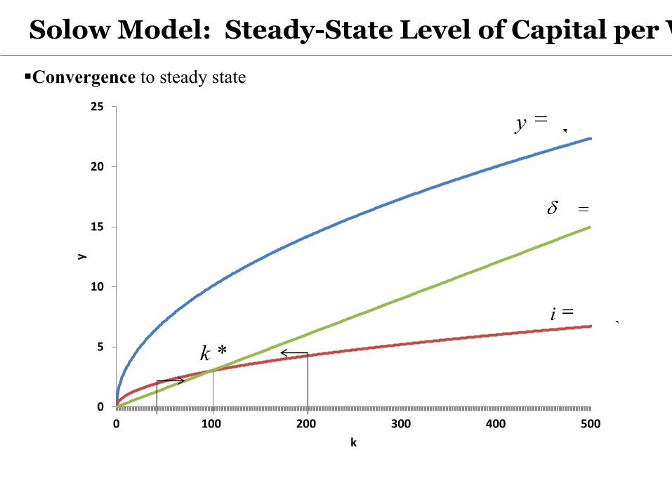
• Economy will remain in the steady state (unless additional channels of growth

are introduced)

• Economy which is not in the steady state will go there => convergence to the

constant level of output per worker over time

• Different economies have different steady state value of capital

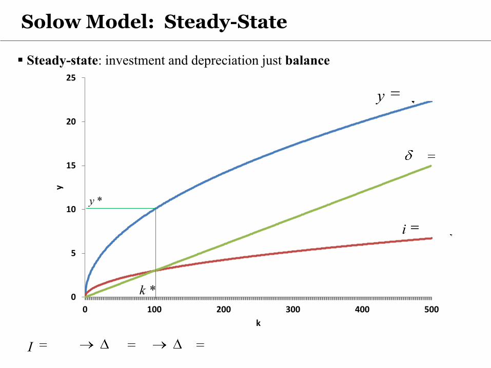
( *) * 0

* * 0

k sf k k

y k y

0

5

10

15

20

25

0 100 200 300 400 500

y

k

y k

0.3i k

0.05k k

Solow Model: Steady-State

0 0I K K k

Steady-state: investment and depreciation just balance

*k

*y

0

5

10

15

20

25

0 100 200 300 400 500

y

k

y k

0.3i k

0.05k k

Solow Model: Steady-State Level of Capital per Worker

Convergence to steady state

*k

Solow Model: Increase in Savings Rate

0

5

10

15

20

25

0 100 200 300 400 500

y

k

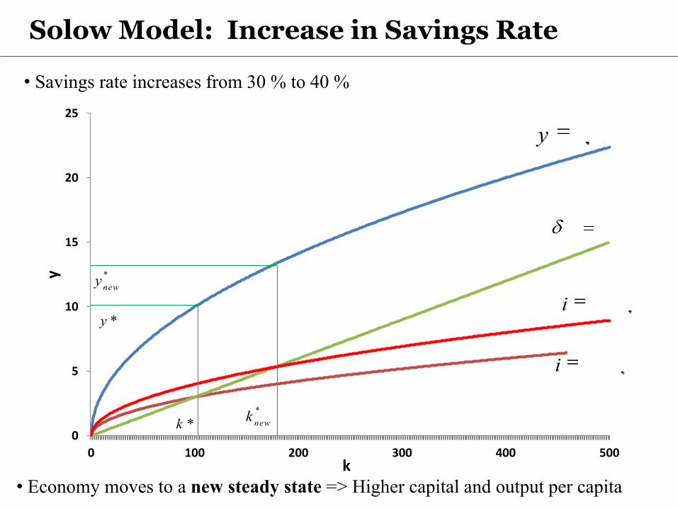
• Savings rate increases from 30 % to 40 %

• Economy moves to a new steady state => Higher capital and output per capita

y k

0.05k k

0.3i k

0.4i k

*k*

newk

*y

*

newy

Solow Model: Steady-State (Cont.)

Implications

Savings rate (s) has no effect on the long-run growth rate of GDP per capita

Increase in savings rate will lead to higher growth of output per capita only

for some time, but not forever.

Saving rate is bounded by interval [0, 1]

Savings rate determines the level of GDP per capita in a long run

Solow Model: The Role of Savings

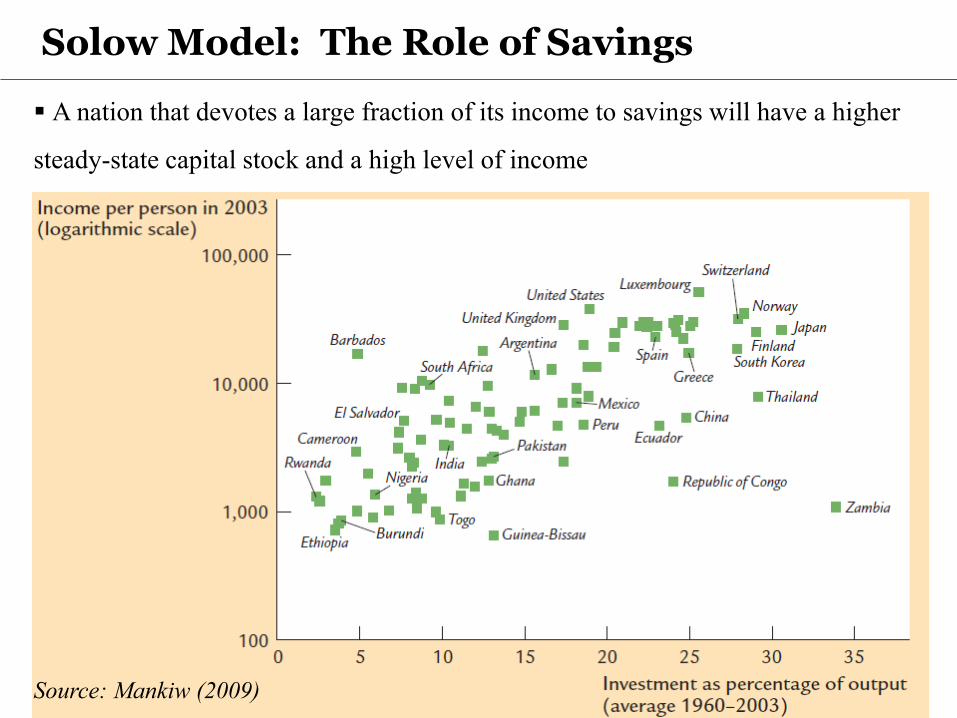
A nation that devotes a large fraction of its income to savings will have a higher

steady-state capital stock and a high level of income

Source: Mankiw (2009)

The Solow-Swan Model: Steady State

Steady state: the long-run equilibrium of the economy

•Savings are just sufficient to cover the depreciation of the capital stock

N!B! Savings rate is a fraction of wage, thus is bounded by the interval [0, 1]

In the long run, capital per worker reaches its steady state for an exogenous s

Increase in s leads to higher capital per worker and higher output per capita

Output grows only during the transition to a new steady state (not sustainable)

Economy will remain in the steady state (no further growth)

Economy which is not in the steady state will go there => Convergence

Government policy response?

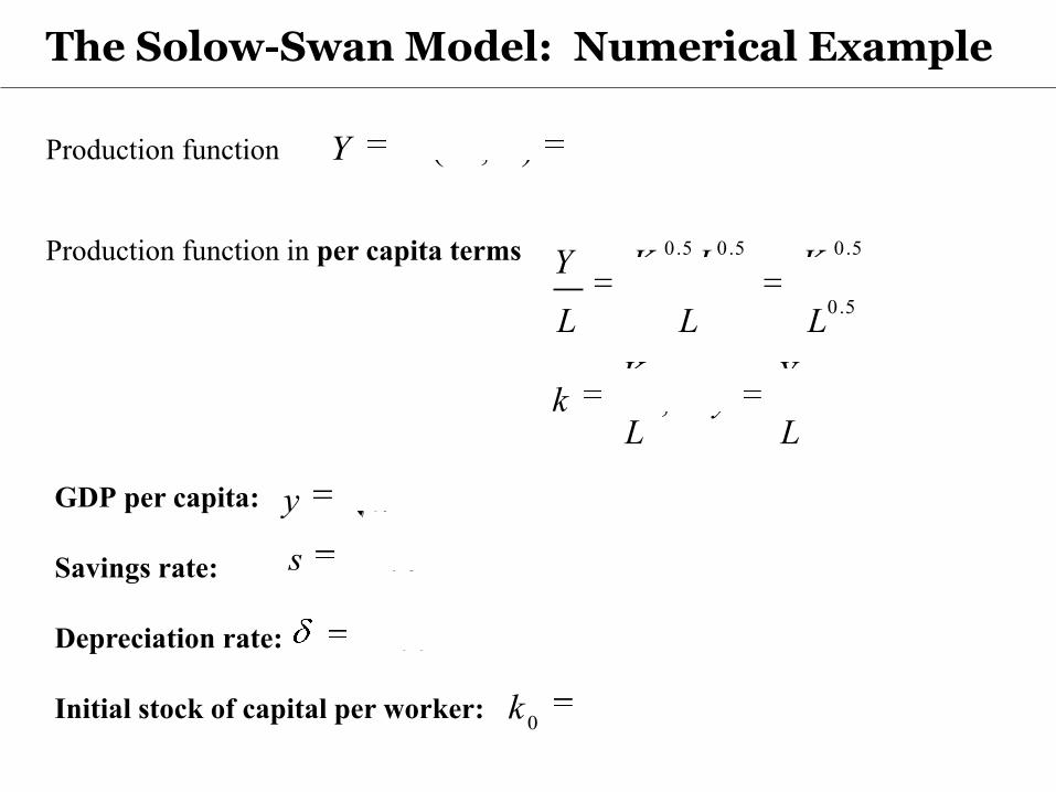
The Solow-Swan Model: Numerical Example

0.5 0.5( , )Y F K L K L

0.5 0.5 0.5

0.5

;

Y K L K

L L L

K Yk y

L L

Production function

Production function in per capita terms

GDP per capita:

Savings rate:

Depreciation rate:

Initial stock of capital per worker:

y k

30%s

10%

04k

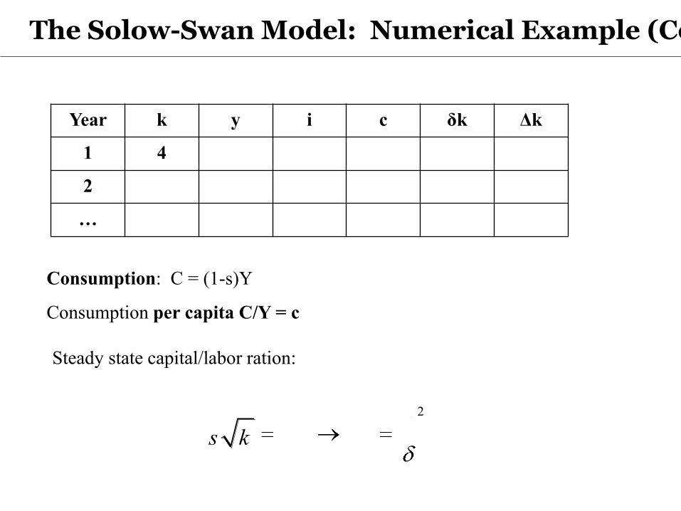
Year k y i c δk Δk

1 4

2

…

Consumption: C = (1-s)Y

Consumption per capita C/Y = c

Steady state capital/labor ration:

2

*

2

ss k k k

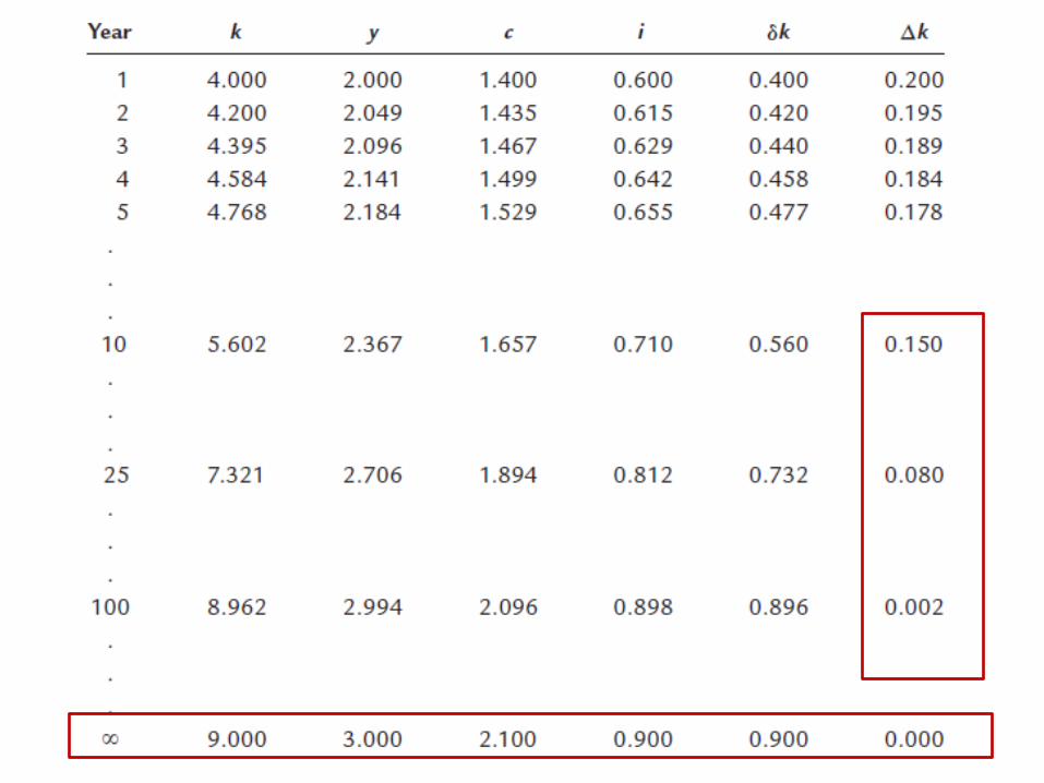
The Solow-Swan Model: Numerical Example (Cont.)

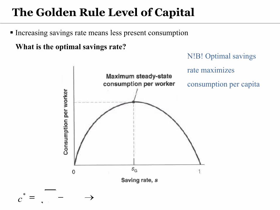
The Golden Rule Level of Capital

Increasing savings rate means less present consumption

What is the optimal savings rate?

* * *maxc k k

N!B! Optimal savings

rate maximizes

consumption per capita

The Solow-Swan Model: Convergence to Steady State

N!B! Regardless of , if two economies have the same s, δ, L, they will

reach the same steady state

0k

• The property of catching-up is known as convergence

• If countries have the same steady state, poorest countries grow faster

• Not much convergence worldwide

Different countries have different institutions and policies

• Conditional convergence: comparison of countries with similar savings rates

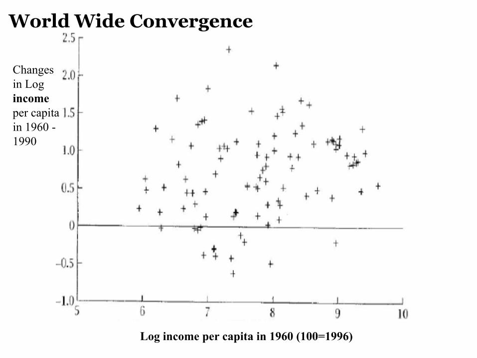
Log income per capita in 1960 (100=1996)

World Wide Convergence

Changes

in Log

income

per capita

in 1960 -

1990

Next class: Solow-Swan Growth Model (Cont.)

N!B! Reading Assignment: Handout “Theories that don’t work”