lecture 2 growth model with exogenous savings: solow...
TRANSCRIPT
Lecture 2
Growth Model with Exogenous Savings:
Solow-Swan Model
Rahul Giri∗
∗Contact Address: Centro de Investigacion Economica, Instituto Tecnologico Autonomo de Mexico (ITAM). E-mail:
As the first step, in order understand the role of proximate causes of economic growth we
develop a simple framework. We take the Solow-Swan model as our starting point. The model
is named after Robert Solow and Trevor Swan, who published two seminal papers in the same
year (1956). Robert Solow developed many applications of the model, and was later awarded the
Nobel prize in economics. This model has not only become the centerpiece of growth theory but
has also shaped the modern macro theory. The central model of macroeconomics before the Solow
model came along was the Harrod-Domar model, which was named after Roy Harrod and Evsey
Domar (Harrod (1939) and Domar (1946)). The Harrod-Domar model focused on unemployment
and growth. The distinguishing feature of the Solow model is the neoclassical aggregate production
function.
1 Model Economy
Consider a closed economy, with a unique final good. The economy is populated by a large number
of households/individuals/agents. All households are identical, so that we can think of this as a
representative household model. The representative household saves a constant exogenous fraction
s ∈ (0, 1) of the disposable income. This assumption is is also used in basic Keynesian models and
the Harrod-Domar model. It is a simplifying assumption which will be relaxed as we move on1.
Like consumers, there are a large number of identical firms and have access to the same production
function for the final good. Another way to say this is that there is a representative firm with a
representative (or aggregate) production function. The aggregate production function is
Y (t) = F (K(t), L(t), A(t)) , (1)
where Y (t) is the total output of final good at time t, K(t) is the capital stock, L(t) is the total
employment, and A(t) is technology at time t. Technology is assumed to be free, i.e. it is publicly
available as a nonexcludable, nonrival good. The implication of this assumption is that A(t) is
freely available to all firms and firms do not have to pay to use this technology.
Assumption 1: The production function F : ℜ3+ → ℜ+ is twice differentiable in K and L,
and satisfies:
FK (K, L, A) ≡∂F (K, L, A)
∂K> 0 , FL (K, L, A) ≡
∂F (K, L, A)
∂L> 0 .
1The Ramsey-Cass-Koopmans model, which is also known as the neoclassical growth model, relaxes this assump-
tion by making s endogenous.
2
FKK (K, L, A) ≡∂2F (K, L, A)
∂K2< 0 , FLL (K, L, A) ≡
∂2F (K, L, A)
∂L2< 0 .
Furthermore, F exhibits constant returns to scale (CRS) in K and L, i.e. F is linearly homogeneous
or homogeneous of degree 1.
Definition: Let K ∈ N . The function g : ℜK+2 → ℜ is homogeneous of degree m in x ∈ ℜ
and y ∈ ℜ if
g (λx, λy, z) = λmg (x, y, z) for all λ ∈ ℜ+ and z ∈ ℜK .
The intuition is that if we double the inputs of capital and labor then the output of the final
good will also double. Another way to think about this assumption is that the economy is large
enough so that the gains from specialization have been exhausted. Linear homogeneous functions
are concave, though not strictly.
Exercise (Euler’s Theorem): Suppose that g : ℜK+2 → ℜ is differentiable in x ∈ ℜ and
y ∈ ℜ, with partial derivatives denoted by gx and gy, and is homogeneous of degree m in x and y.
Then show that:
mg (x, y, z) = gx (x, y, z)x + gy (x, y, z) y ∀ x ∈ ℜ, y ∈ ℜ, and z ∈ ℜK ,
and that gx (x, y, z) and gy (x, y, z) are homogeneous of degree m − 1 in x and y.
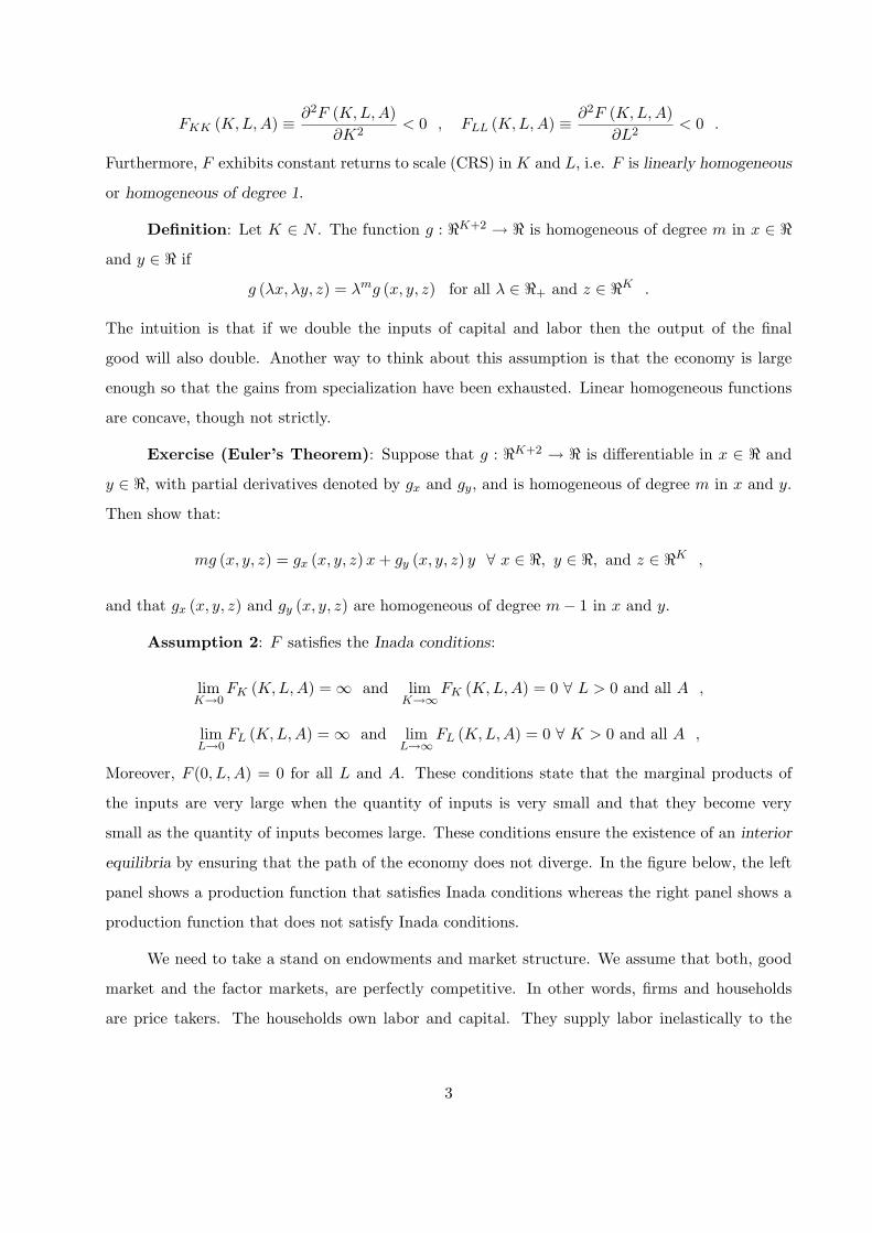
Assumption 2: F satisfies the Inada conditions:
limK→0
FK (K, L, A) = ∞ and limK→∞
FK (K, L, A) = 0 ∀ L > 0 and all A ,
limL→0
FL (K, L, A) = ∞ and limL→∞
FL (K, L, A) = 0 ∀ K > 0 and all A ,
Moreover, F (0, L, A) = 0 for all L and A. These conditions state that the marginal products of
the inputs are very large when the quantity of inputs is very small and that they become very
small as the quantity of inputs becomes large. These conditions ensure the existence of an interior
equilibria by ensuring that the path of the economy does not diverge. In the figure below, the left
panel shows a production function that satisfies Inada conditions whereas the right panel shows a
production function that does not satisfy Inada conditions.
We need to take a stand on endowments and market structure. We assume that both, good
market and the factor markets, are perfectly competitive. In other words, firms and households
are price takers. The households own labor and capital. They supply labor inelastically to the
3
Figure 1: Production Functions and Inada Conditions
firms, i.e. at any time t the demand for labor by firms is equal to the endowment of labor in the
economy2.
L(t) = L(t) . (2)
Capital is also owned by the households, which is rented to the firms. The market clearing for capital
implies that the demand for capital by firms must equal the supply of capital by households.
K(t) = K(t) , (3)
where K(t) is the supply of capital by households and K(t) is the demand by firms. What this
requires is that amount of capital that the firms choose to rent must be equal to the stock of capital
with households resulting from households’ initial endowment of capital and their decision to save
(which is exogenous here). We take the households’ initial stock of capital, K(0) ≥ 0 as given.
We assume that the final good is the numeraire, i.e. price of the final good P (t) = 1. Notice,
2More generally this condition should be written in the complementary slackness form: L(t) ≤ L(t), w(t) ≥ 0 and(
L(t) − L(t))
w(t) = 0. This ensures that labor market clearing does not happen at a negative wage. However, this
is not an issue as long as Assumption 1 holds and factor markets are competitive.
4
that assuming P (t) = 1 at all t is a strong assumption. The same final good at different t is a
different good, just like a bottle of water during water shortage would cost different than during
water abundance. However, when you have securities (in this model capital) which can transfer
one unit of consumption form one date (or state of the world) to another, then all we need is to
keep track of the price of that security. So, in the Solow model this role is fulfilled by the rental
price of capital, R(t). Capital is assumed to depreciate at rate δ, which captures the usual wear
and tear of machinery during the production process. This means that the interest rate faced by
households is net of depreciation, r(t) = R(t) − δ. The law of motion for capital is given by:
K(t) = I(t) − δK(t) , (4)
where I is investment. Since the total amount of the final good can either be consumed or invested,
Y (t) = C(t) + I(t) . (5)
Since aggregate investment must be financed out of aggregate savings, and savings are a fraction s
of the aggregate income,
I(t) = Y (t) − C(t) = sY (t) , (6)
C(t) = (1 − s)Y (t) , (7)
which in turn implies that the law of motion for capital is
K(t) = sY (t) − δK(t) , (8)
Lastly, we need to pin down the factor prices. This comes from the firms side. The objective
of the firms is to maximize profits. Given the assumption of a representative firm the problem is
given by
maxK(t)≥0,L(t)≥0
F (K(t), L(t), A(t)) − R(t)K(t) − w(t)L(t) ,
which combined with the factor market clearing conditions and Assumption 1 gives us the usual
equilibrium relation that factor prices must be equal to the value of marginal products (in this case
equal to marginal products).
w(t) = FL (K(t), L(t), A(t)) and (9)
R(t) = FK (K(t), L(t), A(t)) . (10)
5
Given the constant return to scale aggregate production function, firms in this model do not make
any profits.
Exercise: Given that Assumption 1 holds, show that in equilibrium of the Solow growth
model, firms make no profits, and in particular
Y (t) = w(t)L(t) + R(t)K(t) .
2 Equilibrium and the Steady-State
Equilibrium: For a given sequence of {L(t), A(t)}∞t=0 and an initial capital stock K(0), an equi-
librium path is a sequence of capital stocks, output levels, consumption levels, wages and rental
rates {K(t), Y (t), C(t), w(t), R(t)}∞t=0 such that K(t) satisfies Eq(8), Y (t) is given by Eq(1), C(t)
is given by Eq(7), and w(t) and R(t) are given by Eq(9) and Eq(10), respectively.
To analyze the equilibrium dynamics let us make the following assumptions about the se-
quence of {L(t), A(t)}∞t=0:
L(t) = nL(t) ⇒ L(t) = L(0)ent , (11)
A(t) = gA(t) ⇒ A(t) = A(0)egt , (12)
where L(0) and A(0) are given. We also assume that the nature of technological progress is labor-
augmenting or Harrod-neutral, which then implies that the aggregate production function is
Y (t) = F (K(t), A(t)L(t)) .
Define k = K/AL as capital per unit of effective labor, where the product of A and L captures the
units of effective of labor. Similarly, define f(k) = y = Y/AL is output per unit of effective labor.
Then
k(t) =K(t)
A(t)L(t)−
K(t)
(A(t)L(t))2
(
A(t)L(t) + L(t)A(t))
,
⇒ k(t) =K(t)
A(t)L(t)−
K(t)
A(t)L(t)
(
L(t)
L(t)+
A(t)
A(t)
)
.
Then substituting for K(t) from the law of motion gives us the fundamental law of motion of the
Solow model.
k(t) = sf(k(t)) − (n + g + δ)k(t) . (13)
6
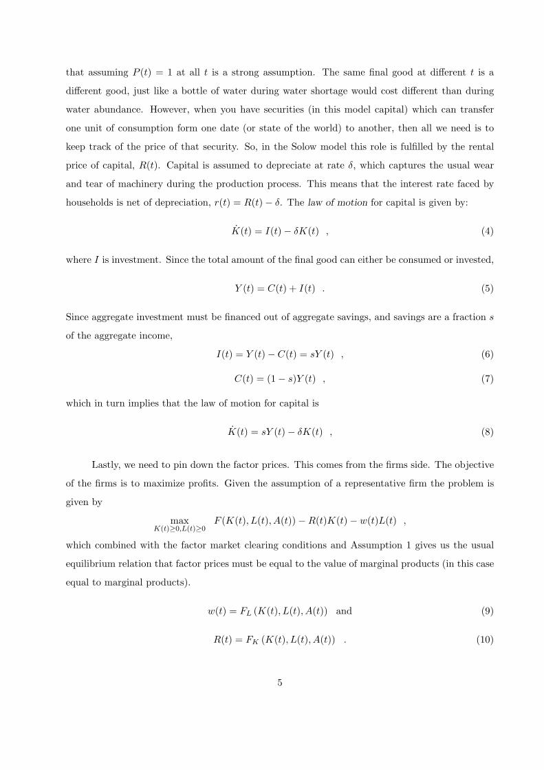
This equation states that the rate of change of the capital stock per unit of effective labor is the
difference between two terms. The first term, sf(k), is actual investment per unit of effective labor.
The second term, (n + g + δ)k is break-even investment, i.e. the amount of investment that must
be done to keep k at its existing level. Investment is needed to prevent k from falling because the
existing capital deprecates at rate δ, which is captured by δk term, and also because the quantity
of effective labor is also growing at rate (n+ g), which is captured by the term (n+ g)k. Therefore,
when the actual investment per unit of effective labor exceeds the break-even investment k rises,
and vice-versa. Moreover, when the two are equal k is constant. This is depicted in the figure
below. The figure plots the two terms of the right-hand side of the fundamental law of motion
as functions of k. Since F (0, L, A) = 0 it implies that f(0) = 0, and therefore actual investment
Figure 2: Actual investment and break-even investment
and break-even investment are equal at k = 0. Furthermore, the Inada conditions imply that as k
goes to zero fk(k) becomes very large. Therefore sf(k) is steeper than break even investment line
around k = 0, and actual investment is larger than break-even investment. The Inada conditions
also imply that fk(k) falls to zero as k becomes very large. As a result, at some point the slope of
7
the actual investment curve becomes less than the slope of the break-even investment line, implying
that the two lines must eventually cross. Finally, due to diminishing returns, fkk < 0, the two lines
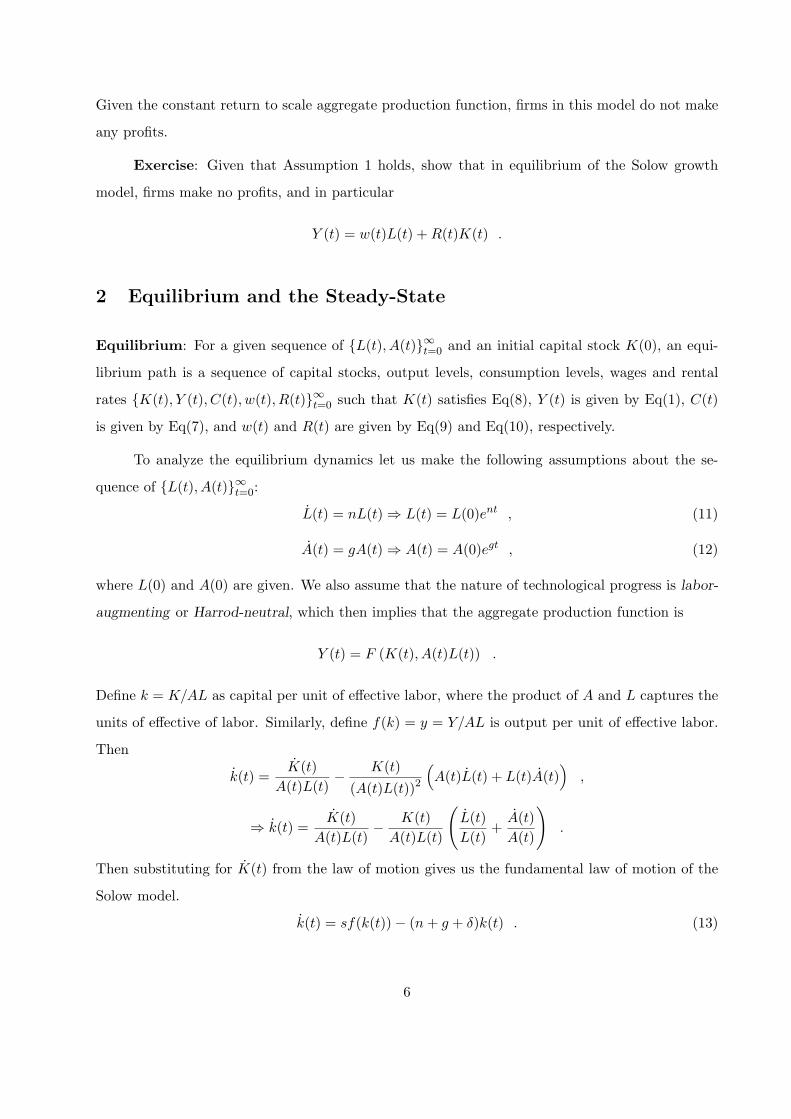
intersect only once. Let k∗ be the value where actual investment equals break-even investment, or
in other words there is no change in capital per unit of effective labor, k = 0. This value of k is
also called the steady state value of k.
The next figure shows that the economy converges to k∗ regardless of where it starts. When
k is less than k∗ actual investment exceeds break-even investment as a result k is positive. When
k is greater than k∗ the actual investment is less than break-even investment and therefore k is
negative. Finally for k = k∗, k = 0.
Figure 3: Steady State
2.1 The Balanced Growth Path
How are output, capital and consumption growing in this economy when k = k∗. We know that L
and A are growing at exogenously given rates - n and g, respectively. The capital stock K = ALk,
and since k is constant at k∗, the aggregate capital stock of the economy is growing at the rate
8
(n + g). With both capital and effective labor growing at the same rate (n + g), the assumption of
constant returns to scale implies that aggregate output is also growing at the rate (n + g). Since
consumption is (1 − s)Y , where s is constant, consumption also grows at the same rate as output.
Finally, capital per unit of labor, K/L, and output per unit of labor, Y/L, grow at the rate g.
Thus, the Solow model implies that regardless of its starting point, the economy converges to a
balanced growth path, where each variable grows at a constant rate.
At this point we also need to discuss our assumption that technological change is labor-
augmenting. This is a restriction that is required for the existence of a balanced growth path.
Other types of technological change - Hicks-neutral (unbiased technological change) and capital-
augmenting technical change - are not consistent with a balanced growth path. For a proof look at
Uzawa (1961). Notice that off the balanced growth path technological change is no longer required
to labor-augmenting.
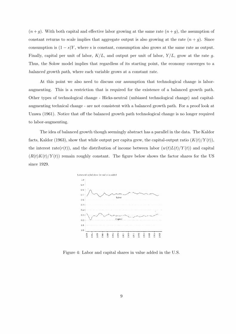
The idea of balanced growth though seemingly abstract has a parallel in the data. The Kaldor
facts, Kaldor (1963), show that while output per capita grew, the capital-output ratio (K(t)/Y (t)),
the interest rate(r(t)), and the distribution of income between labor (w(t)L(t)/Y (t)) and capital
(R(t)K(t)/Y (t)) remain roughly constant. The figure below shows the factor shares for the US
since 1929.
Figure 4: Labor and capital shares in value added in the U.S.
9
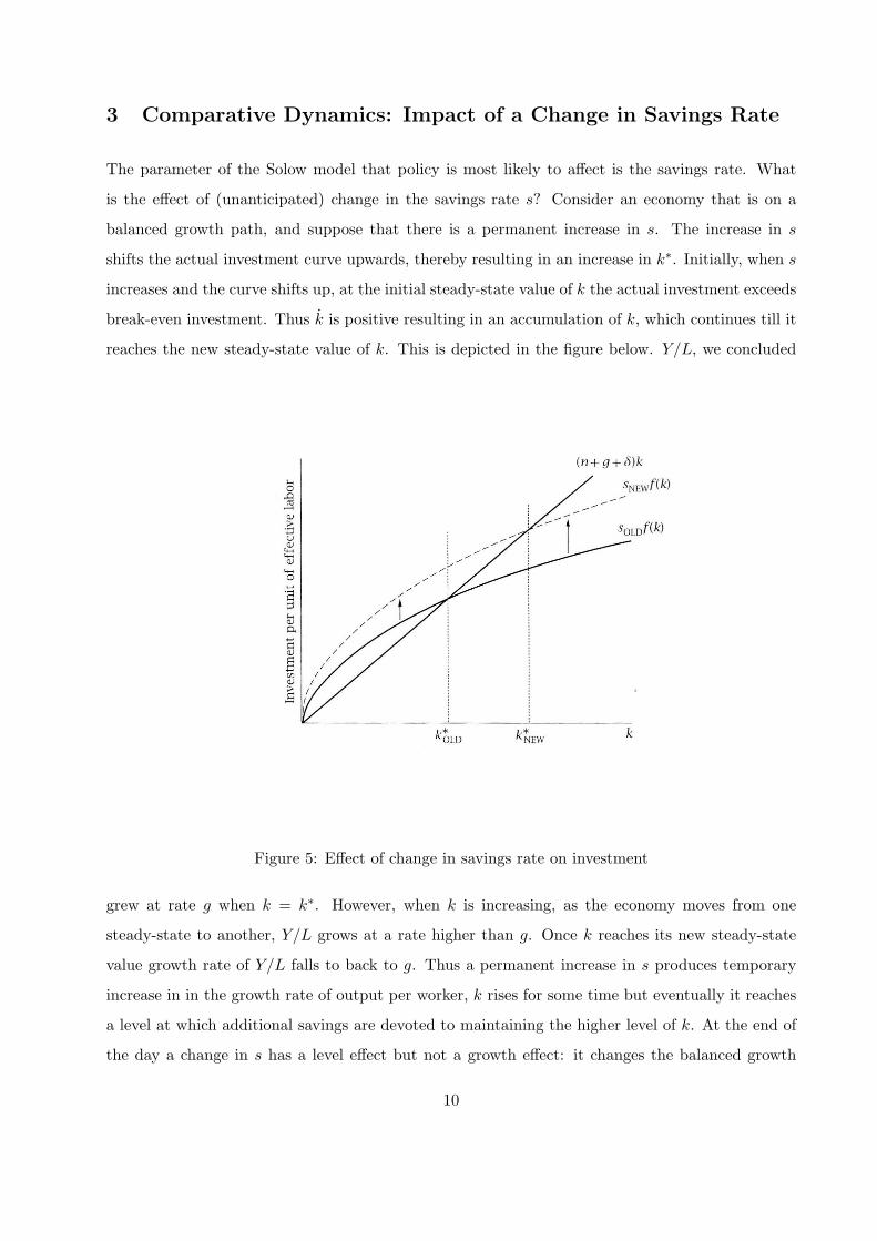
3 Comparative Dynamics: Impact of a Change in Savings Rate
The parameter of the Solow model that policy is most likely to affect is the savings rate. What
is the effect of (unanticipated) change in the savings rate s? Consider an economy that is on a
balanced growth path, and suppose that there is a permanent increase in s. The increase in s
shifts the actual investment curve upwards, thereby resulting in an increase in k∗. Initially, when s
increases and the curve shifts up, at the initial steady-state value of k the actual investment exceeds
break-even investment. Thus k is positive resulting in an accumulation of k, which continues till it
reaches the new steady-state value of k. This is depicted in the figure below. Y/L, we concluded
Figure 5: Effect of change in savings rate on investment
grew at rate g when k = k∗. However, when k is increasing, as the economy moves from one
steady-state to another, Y/L grows at a rate higher than g. Once k reaches its new steady-state
value growth rate of Y/L falls to back to g. Thus a permanent increase in s produces temporary
increase in in the growth rate of output per worker, k rises for some time but eventually it reaches
a level at which additional savings are devoted to maintaining the higher level of k. At the end of
the day a change in s has a level effect but not a growth effect: it changes the balanced growth
10
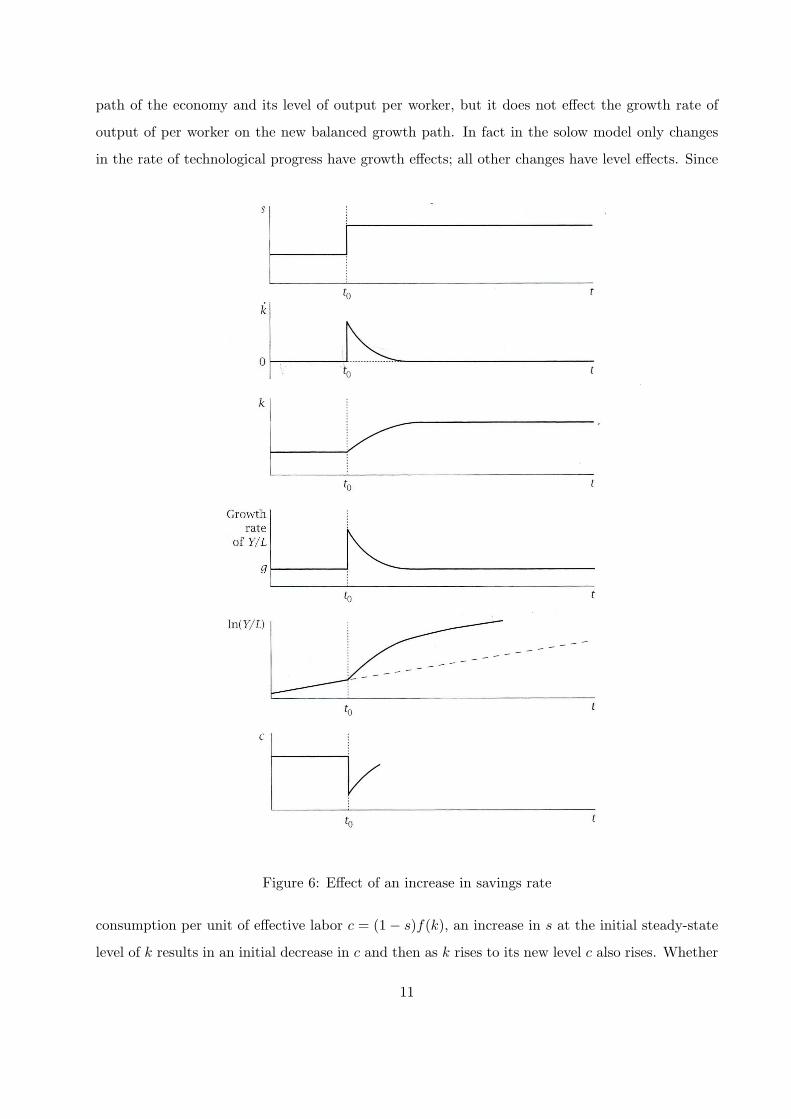
path of the economy and its level of output per worker, but it does not effect the growth rate of
output of per worker on the new balanced growth path. In fact in the solow model only changes
in the rate of technological progress have growth effects; all other changes have level effects. Since
Figure 6: Effect of an increase in savings rate
consumption per unit of effective labor c = (1 − s)f(k), an increase in s at the initial steady-state
level of k results in an initial decrease in c and then as k rises to its new level c also rises. Whether
11
or not c exceeds its original level can be seen by writing down the expression for consumption per
unit of effective labor. Steady-state consumption is given by:
c∗ = f(k∗) − (n + g + δ)k∗ ,
⇒∂c∗
∂s= [fk (k∗(s, n, g, δ)) − (n + g + δ)]
∂k∗(s, n, g, δ)
∂s.
An increase in s raises k∗. Thus, c∗ will rise in response to an increase in s if the marginal product
of capital, fk, is greater than (n + g + δ). Intuitively when k rises investment must increase by
(n + g + δ) times k in order to sustain the new level of k. If fk is less than (n + g + δ), then the
additional output from a higher k is not enough to support the higher level of k. As a result c must
decline in the long run to maintain the stock of capital. On the other hand, if fk exceeds (n+g+δ)
there is more than enough output to support the higher level of k, and therefore c increases in the
long run. However, if the steady-state value of k to start with is such that fk = (n + g + δ) then
a marginal change in s does not change c. This value of k∗ is called the golden rule level of the
capital stock. At the golden rule level of capital consumption is at its maximum level. Since s is
exogenous in the Solow model, there is no guarantee that k∗ will be at its golden rule level. This
cases are depicted in the figure below.
4 Quantitative Implications of the Model
Let us do a simple assessment of the Solow model in terms of its ability to match aspects of the
growth facts we have discussed.
4.1 Steady State: Quantitative Importance of Savings Rate in Affecting Income
Per Capita in the Long Run
In our discussions we saw that income per capita varies significantly across countries. Can the
savings rate have a quantitatively important impact on income per capita so as to explain such
large income differences? The long run effect of a change in savings rate on output per unit of
effective labor is given by:∂y∗
∂s= fk (k∗)
∂k∗(s, n, g, δ)
∂s.
At k = k∗, sf (k∗(s, n, g, δ)) = (n + g + δ)k∗(s, n, g, δ), which implies that
∂k∗
∂s=
f (k∗)
(n + g + δ) − sfk (k∗),
12
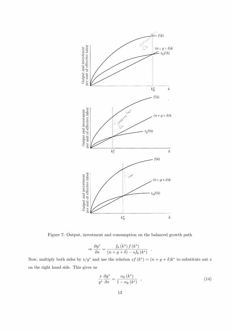
Figure 7: Output, investment and consumption on the balanced growth path
⇒∂y∗
∂s=
fk (k∗) f (k∗)
(n + g + δ) − sfk (k∗).
Now, multiply both sides by s/y∗ and use the relation sf (k∗) = (n + g + δ)k∗ to substitute out s
on the right hand side. This gives us
s
y∗∂y∗
∂s=
αk (k∗)
1 − αk (k∗), (14)
13
where αk (k∗) = k∗fk (k∗) /f (k∗) is the elasticity of output with respect to capital at k = k∗.
Furthermore, since fk = R(t), αk (k∗) is also interpreted as the share of capital in total income
on the balanced growth path. This share in most countries has been found to be about one-third.
This implies that the elasticity of output with respect to the savings rate is about one-half. Thus,
a 10% increase in savings rate increases per worker output in the long run by 5% relative to the
path it would have followed. For a 50% change in savings rate y∗ rises by only 22%. Thus, big
changes in savings rate have only a moderate effect on the level of output on the balanced growth
path.
4.2 Transition Dynamics: Speed of Convergence
How quickly do model variables move from one equilibrium to another in response to some ex-
ogenous change? More specifically, how rapidly does k approach k∗? To do this we take the
fundamental law of motion of the Solow model and take Taylor-series expansion around k = k∗.
This gives
k ≈ −λ (k − k∗) , (15)
where
λ = −
[
∂k(k)
∂k
]
k=k∗
= (1 − αk (k∗)) (n + g + δ) .
Since k is positive when k is slightly below k∗ and negative when it is slightly above k∗, ∂k(k)/∂k
is negative implying that λ is positive. Eq(15) implies that in the neighborhood of the balanced
growth path, k converges to k∗ at a speed proportional to its distance from k∗. This then gives us
the following expression
k(t) ≈ k∗ + exp−λt (k(0) − k∗) , (16)
where k(0) is the initial value of k. Similarly, we can also show that y(t)− y∗ ≈ exp−λt (y(0) − y∗).
Now let us put some numbers (per year). Typically, (n + g + δ) is around 5− 6%: n is 1 percent, g
is proxied by taking growth rate of output per worker, which is around 2 percent, and δ is around
5 percent. Taking α to be one-third implies that λ is about 5.6 percent, which means that k and
y move about 5.6 percent of the remaining distance towards k∗ and y∗ each year. An economy
starting from some k(0) and y(0) would be halfway to its balanced growth path when e−λt = 0.5.
This would mean that it would take an economy about 12.5 years to reach the half-way point to its
balanced growth path. This speed of convergence is too high to account for the empirical evidence;
λ, of 1.5 to 3 percent fits better with the data.
14
Note that by assuming α to be constant we impose the restriction that the production function
is Cobb-Douglas. This results in two properties of the convergence coefficient. First, the saving
rate, s, does not affect λ. This is because of two offsetting forces that exactly cancel in the Cobb-
Douglas case. Given k, a higher savings rate leads to greater investment and, therefore, to a faster
speed of convergence. But, a higher savings rate also raises the steadt state capital, k∗, and thereby
lowers the average product of capital. This reduces the speed of convergence. The second thing to
note is that the level of technology or efficiency of the economy, A, does not affect λ. Changes in
A, like changes in s, have two offsetting effects on the convergence speed, and these effect exactly
cancel in the Cobb-Douglas case.
Furthermore, due to the negative relation between current output and transition growth in
per capita terms, poor countries grow faster than the rich ones if they are on the transition path
of growth, and the speed of this catch-up is governed by the coefficient λ. However, this catch-up
stops once they reach the steady state and every country should grow at the same rate g purely
coming from technological progress. At that point inequality in per capita incomes across countries
persists at a constant level.
4.3 Can the Solow Model Explain Cross-Country Income Differences?
In the Solow model there are two factors that lead to differences in in output per worker across
countries: differences in capital per worker (K/L) and differences in technology (A). However,
we have seen that only growth in technology can lead to sustained growth in output. Due to
diminishing return to capital, changes in capital labor ratio have very modest effect on output per
worker.
Suppose we want to account for difference of a factor of X in per worker output across two
countries. Then difference in log output per worker is log X. Since the elasticity of output per
worker with respect to capital per worker is αk, log capital per worker must differ by (log X) /αk.
That is capital per worker differs by a factor of exp(logX)/αk , or X1/αk . As we have seen, output
per worker in the richest countries exceeds that in the poorest countries by a factor of 30. With
αk = 1/3, this would imply that capital per worker in the richest countries exceeds that in the
poorest countries by a factor of 27000. The data shows that capital per worker is only about 20 to
30 times larger in the richest countries as compared to the poorest countries. Therefore, differences
in capital per worker are far smaller than those needed to account for the differences in output per
worker.
15
The other factor that can explain these income differences is technology. However, in the
model technology grows at an exogenous rate. Thus, the variable that is the central force behind
growth in per capita incomes is itself exogenous! Moreover, the model does not tell us much about
how to think about it. Technically A captures the effect on output of all factors except capital
and labor. These other factors could include technology, education, skills, strength of property
rights, quality of infrastructure, cultural attitudes towards entrepreneurship and work, etc.. It is
essentially a black box!
Exercise: Suppose the aggregate production function is Cobb-Douglas:
F (t) = K(t)α (A(t)L(t))1−α .
Replicate the results on the growth rate of k, y, c, K/L, Y/L. Also, obtain an expression for k∗ and
y∗.
5 References
1. Domar, Evsey D. (1946), “Capital Expansion, Rate of Growth and Employment”, Economet-
rica 14: 137-147.
2. Harrod, Roy (1939), “An Essay in Dynamic Theory”, Economic Journal 49: 14-33.
3. Kaldor, Nicholas (1963), “Capital Accumulation and Economic Growth”, In Proceedings of a
Conference Held by the International Economics Association, Friedrich A. Lutz and Douglas
C. Hague (editors). London: Macmillan.
4. Solow, Robert M. (1956), “A Contribution to the Theory of Economic Growth”, Quarterly
Journal of Economics 70: 65-94.
5. Swan, Trevor W. (1956), “Economic Growth and Capital Accumulation”, Economic Record
32: 334-361.
6. Uzawa, Hirofumi (1961), “Neutral Inventions and the Stability of the Growth Equilibrium!”,
Review of Economic Studies 28: 117-124.
16