The Solow Model

Prof. Lutz Hendricks

Econ520

January 26, 2017

1 / 28

Issues

The production model measures the proximate causes of incomegaps.Now we start to look at deep causes.

The Solow model answers questions such as:

1. Why do countries lack capital?2. How much of cross-country income gaps is due to differences

in saving rates?3. Does capital accumulation drive long-run growth?

2 / 28

Objectives

At the end of this section you should be able to

1. Derive properties of the Solow model: steady state, effects ofshocks, ...

2. Graph the dynamics of the Solow model.3. Explain why the contribution of capital (saving) to

cross-country output gaps is small.

3 / 28

The Solow Model

We add just one piece to the production model:

I an equation that describes how capital is accumulated overtime through saving.

4 / 28

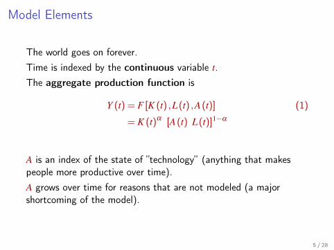
Model Elements

The world goes on forever.Time is indexed by the continuous variable t.The aggregate production function is

Y (t) = F [K (t) ,L(t) ,A(t)] (1)

= K (t)α [A(t) L(t)]1−α

A is an index of the state of ”technology” (anything that makespeople more productive over time).A grows over time for reasons that are not modeled (a majorshortcoming of the model).

5 / 28

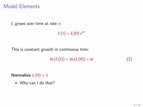
Model Elements

L grows over time at rate n:

L(t) = L(0) ent

This is constant growth in continuous time:

ln(L(t)) = ln(L(0)) + nt (2)

Normalize L(0) = 1

I Why can I do that?

6 / 28

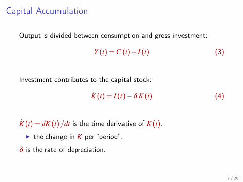
Capital Accumulation

Output is divided between consumption and gross investment:

Y (t) = C (t) + I (t) (3)

Investment contributes to the capital stock:

K̇ (t) = I (t)−δ K (t) (4)

K̇ (t) = dK (t)/dt is the time derivative of K (t).

I the change in K per “period”.

δ is the rate of depreciation.

7 / 28

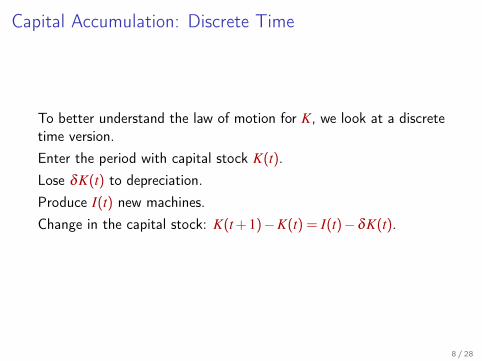
Capital Accumulation: Discrete Time

To better understand the law of motion for K, we look at a discretetime version.Enter the period with capital stock K(t).Lose δK(t) to depreciation.Produce I(t) new machines.Change in the capital stock: K(t + 1)−K(t) = I(t)−δK(t).

8 / 28

Capital Accumulation: Discrete Time

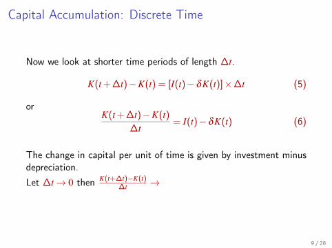
Now we look at shorter time periods of length ∆t.

K(t + ∆t)−K(t) = [I(t)−δK(t)]×∆t (5)

orK(t + ∆t)−K(t)

∆t= I(t)−δK(t) (6)

The change in capital per unit of time is given by investment minusdepreciation.Let ∆t→ 0 then K(t+∆t)−K(t)

∆t →

9 / 28

Choices

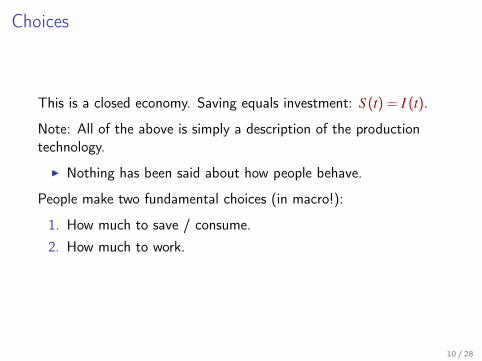
This is a closed economy. Saving equals investment: S (t) = I (t).

Note: All of the above is simply a description of the productiontechnology.

I Nothing has been said about how people behave.

People make two fundamental choices (in macro!):

1. How much to save / consume.2. How much to work.

10 / 28

Choices

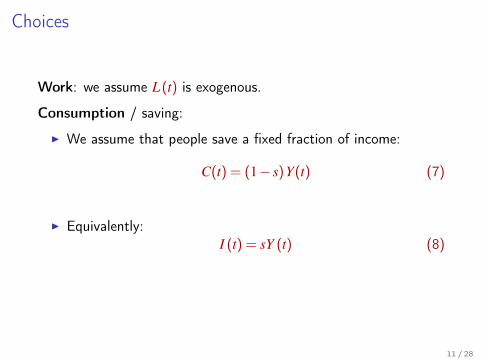
Work: we assume L(t) is exogenous.

Consumption / saving:

I We assume that people save a fixed fraction of income:

C(t) = (1− s)Y(t) (7)

I Equivalently:I (t) = sY (t) (8)

11 / 28

Model Summary

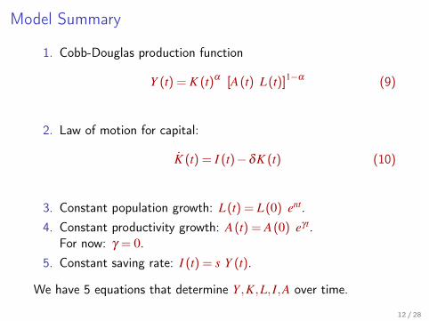
1. Cobb-Douglas production function

Y (t) = K (t)α [A(t) L(t)]1−α (9)

2. Law of motion for capital:

K̇ (t) = I (t)−δK (t) (10)

3. Constant population growth: L(t) = L(0) ent.4. Constant productivity growth: A(t) = A(0) eγt.

For now: γ = 0.5. Constant saving rate: I (t) = s Y (t).

We have 5 equations that determine Y,K,L, I,A over time.

12 / 28

The Law of Motion for Capital

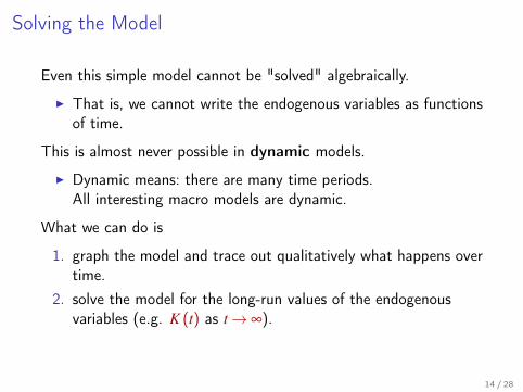
Solving the Model

Even this simple model cannot be "solved" algebraically.

I That is, we cannot write the endogenous variables as functionsof time.

This is almost never possible in dynamic models.

I Dynamic means: there are many time periods.All interesting macro models are dynamic.

What we can do is

1. graph the model and trace out qualitatively what happens overtime.

2. solve the model for the long-run values of the endogenousvariables (e.g. K (t) as t→ ∞).

14 / 28

The Solow Diagram

I We condense the model into a single equation in K.I It will be a dynamic equation that tells us how K changes over

time as a function of K.I Then we graph the equation.

15 / 28

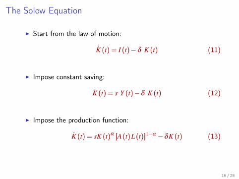
The Solow Equation

I Start from the law of motion:

K̇ (t) = I (t)−δ K (t) (11)

I Impose constant saving:

K̇ (t) = s Y (t)−δ K (t) (12)

I Impose the production function:

K̇ (t) = sK (t)α [A(t)L(t)]1−α −δK (t) (13)

16 / 28

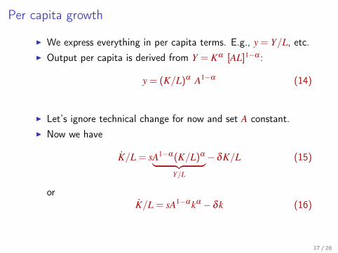
Per capita growth

I We express everything in per capita terms. E.g., y = Y/L, etc.I Output per capita is derived from Y = Kα [AL]1−α :

y = (K/L)α A1−α (14)

I Let’s ignore technical change for now and set A constant.I Now we have

K̇/L = sA1−α (K/L)α︸ ︷︷ ︸Y/L

−δK/L (15)

orK̇/L = sA1−αkα −δk (16)

17 / 28

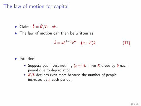
The law of motion for capital

I Claim: k̇ = K̇/L−nk.I The law of motion can then be written as

k̇ = sA1−αkα − (n + δ )k (17)

I Intuition:I Suppose you invest nothing (s = 0). Then K drops by δ each

period due to depreciation.I K/L declines even more because the number of people

increases by n each period.

18 / 28

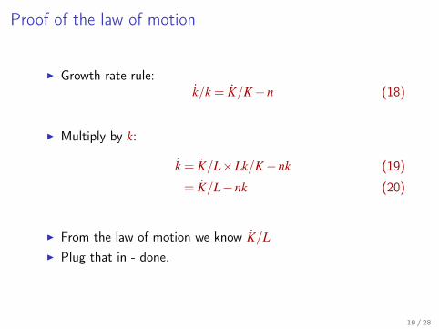
Proof of the law of motion

I Growth rate rule:k̇/k = K̇/K−n (18)

I Multiply by k:

k̇ = K̇/L×Lk/K−nk (19)

= K̇/L−nk (20)

I From the law of motion we know K̇/LI Plug that in - done.

19 / 28

Digression: What modern macro would do

I Modern macro would replace the constant saving rate with anoptimizing household.

I Households maximize utility of consumption, summed overall dates.

I They choose time paths of c(t) and K (t).I The saving rate would be endogenous and depend on

I the interest rate (marginal product of K)I productivityI population growthI expectations of all future variables.

I What do we gain from this complication?

20 / 28

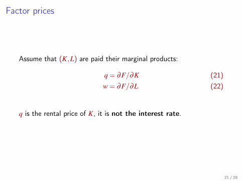
Factor prices

Assume that (K,L) are paid their marginal products:

q = ∂F/∂K (21)w = ∂F/∂L (22)

q is the rental price of K, it is not the interest rate.

21 / 28

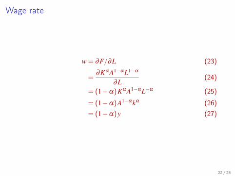
Wage rate

w = ∂F/∂L (23)

=∂KαA1−αL1−α

∂L(24)

= (1−α)KαA1−αL−α (25)

= (1−α)A1−αkα (26)= (1−α)y (27)

22 / 28

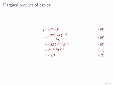
Marginal product of capital

q = ∂F/∂K (28)

=∂Kα (AL)1−α

∂K(29)

= α (AL)1−α Kα−1 (30)

= αA1−αkα−1 (31)= αy/k (32)

23 / 28

The Interest Rate

What is an interest rate?

The interest rate answers the question:

24 / 28

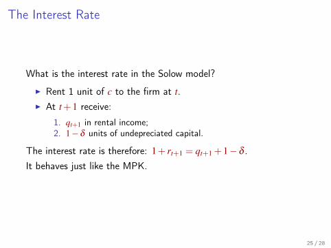
The Interest Rate

What is the interest rate in the Solow model?

I Rent 1 unit of c to the firm at t.I At t + 1 receive:

1. qt+1 in rental income;2. 1−δ units of undepreciated capital.

The interest rate is therefore: 1 + rt+1 = qt+1 + 1−δ .It behaves just like the MPK.

25 / 28

Summary

Law of motion for capital:

k̇ = sA1−αkα − (n + δ )k (33)

Wage rate:w = (1−α)A1−αkα (34)

Interest rate:

r = q−δ (35)

= αA1−αkα−1 (36)

26 / 28

Reading

I Jones (2013), ch. 2I Blanchard and Johnson (2013), ch. 11

Further Reading:

I Romer (2011), ch. 1I Barro and Martin (1995), ch. 1.2

27 / 28

References I

Barro, R. and S.-i. Martin (1995): “X., 1995. Economic growth,”Boston, MA.

Blanchard, O. and D. Johnson (2013): Macroeconomics, Boston:Pearson, 6th ed.

Jones, Charles; Vollrath, D. (2013): Introduction To EconomicGrowth, W W Norton, 3rd ed.

Romer, D. (2011): Advanced macroeconomics, McGraw-Hill/Irwin.

28 / 28