Time Series Tests of the Solow Growth Model

November, 2005

David Papell, University of Houston

Ruxandra Prodan, University of Alabama

Correspondence to:

David Papell, tel. (713) 743-3807, email: dpapell@mail.uh.edu, Department of Economics,

University of Houston, Houston, TX 77204-5019.

Ruxandra Prodan, tel. (205) 348-8985, email: rprodan@cba.ua.edu, Department of Economics,

University of Alabama, Tuscaloosa, AL 35405.

We propose a new methodology in order to study the stability of output growth over 135

years for 19 OECD countries and 7 Asian countries. Previous research on economic

growth can be categorized in three hypothesis: first, the level and the growth rate of

long run income per capita is constant, second, policy changes have transitory effect on

the growth rate of the economy and permanent effect on the income level and third,

policy changes have permanent effect on the economy’s long run growth rate and

income level. Our innovation consists in the fact that we formally test these hypotheses

using time series tests techniques. We find evidence of constant income levels and

growth rates for 2 countries which were the least affected by wars, US and Canada. For

the second group of 7 OECD countries, strongly affected by the World War II, we find

constant growth rate but a permanent change in the income level after a shock, showing

evidence towards semi-endogenous growth models. Finally, there is a third group of 11

countries (all Asian countries and some European countries) where we find permanent

changes in growth rate and income level after a shock, showing evidence towards

endogenous growth models.

“Consider the following simple exercise. An economist living in the year 1929 (who has

miraculous access to historical per capita GDP data) fits a simple linear trend to the

natural log of per capita GDP for the United States from 1880 to 1929 in an attempt to

forecast per capita GDP today, say in 1987. How far off would the prediction be?”

Charles Jones

1. Introduction

In his 1995 article, Jones argues that the average U.S. growth rate has been stable over

the last century, being well described by a process with a constant mean and little persistence.

However, this remains a puzzle even from the standpoint of a neoclassical growth model:

the documented significant increase in R&D intensity or time spent accumulating skills through

formal education in United States should generate temporarily high growth rates and long run

“level effects”, but the evidence looks like an economy that is fluctuating around its balanced

growth path.1 Furthermore, in many endogenous growth models, such policy changes should

lead to permanent increase in the growth rate: in models of Romer (1986), Lucas (1988) and

Rebelo (1991) where investment in human and physical capital is the engine of growth or in

models of Romer (1990) and Aghion and Howitt (1992) where the growth rate of the economy is

an increasing function of the research effort.

To reconcile these facts, Jones (1995, 2002, 2004) proposes an ideas-based model, in

which ideas are nonrivalrous, implying that output per capita is an increasing function, in the

long run, of the number of researchers in the economy, which in turn depends on the size of the

population. In this setting policy changes will have no effect on the long run growth rate but only

on the long-run level of per capita income (semi-endogenous growth model).2 Jones argues that

these models exhibit “weak” scale effects versus first-generation idea-based growth models

1 The neoclassical growth model (Solow, 1956) postulates stable equilibrium with a long run constant income

growth rate. Following changes in variables affected by government policy, specifically savings and investment, the

growth rate of the economy rises temporarily and then returns to its original value, but the level of income is

permanently higher as a result. 2 The long-run growth rate in these models is generally an increasing function of the growth rate of research effort,

which depends on the population growth rate of the countries contributing to the world research. But this growth rate

is taken to be exogenous in these models, producing the policy-invariance results.

which exhibit “strong” scale effects. Also, he argues that these are better representations for the

trends in the data and also they not rely on the strong assumption of linearity, which has been

subject to several critiques.3 He also gives several possible explanations for the US stable growth

rate: First, either nothing in the US experience had large persistent effect on the growth rate or

else, that persistent effects have been offsetting each other and finally that US growth is

generated by a sequence of transition dynamics at a constant rate that is higher than the steady

state rate.4 A straightforward implication of this result is that growth rates could slow down at

some point in the future, when the transition period ended.

Jones (1995) has previously applied the same rationale when examining the growth rates

in several advanced OECD countries. While a stylized fact shows that the investment rates in

most of these countries have dramatically increased, Jones (1995) documents that growth rates of

GDP per capita have remained roughly constant over the last century over the post-World War

era for these countries5.

There is a huge amount of empirical work, using cross-country and time series

methodology, which tried to make a clear choice between neoclassical and endogenous type

growth models but failed to arrive to a common consensus. Studies by Lee (1988), Kremer

(1993), McGraham (1998), have argued in favor of endogenous growth models with “strong”

scale effects.6 Contrarily, Mankiew et all (1992), Karras (2001) and several other authors found

significant evidence in agreement with the neoclassical growth model. However, there has not

been too much research devoted to study the relevance of “weak” scale effects. As argued in

Jones (2004) the most apparent lack of support for the hypothesis of “weak” scale effects comes

from the fact that most populous countries of the world, as China and India are among the

poorest while some of the smallest countries, like Hong-Kong and Luxembourg are among the

richest. The rich countries have benefited tremendously from ideas around the world and the

poor countries have very different levels of human capital, policies, institutions and property

rights, so the evidence is not clear. On the other hand, cross-country studies that have explicitly

3 The law of motion for human and physical capital accumulation is assumed to be linear and the idea production

function is assumed to be a linear differential equation. 4 Jones (2002) argues that 80% of the US growth in post-war period is due to the transition dynamics associated with

increases in educational attainment or increase in the world R&D intensity. They seem to rise smoothly, generating

an approximate stable growth path. 5 This provides evidence against AK models.

6 There are many other studies that test endogenous growth models, where the engine is growth in investment, etc

but for the purpose of this paper we will focus on models that test growth models where the growth engine is R&D.

control for differences in international trade and institution quality, such as Backus, Kehoe and

Kehoe (1992), Frankel and Romer (1999), Jones (2001) and Alcala and Ciccone (2002) have

found an important role for the “weak” scale effects.

This paper proposes a new methodology in order to study the stability of output growth

over 135 years for 19 OECD countries and 7 Asian countries. Previous research on economic

growth theory can be categorized in three hypothesis: “The Jones-Weil-Summers hypothesis”7, is

that the level of per capita GDP can be represented by a simple trend, “The Jones-Solow

hypothesis” is that after a shock the growth rate of the economy rises temporarily and then

returns to its original value, but the level of income is permanently higher and “The Romer

hypothesis” is that policy changes have permanent effects on economy’s long run growth rate.

Our innovation consists in the fact that we formally test these hypotheses using time series tests

techniques.

Tests for structural change in univariate time series provide a natural framework for

investigating the stylized fact of constant output growth. A common characteristic to all theses

countries is that they experience downward trends in their GDP per capita during the World War

II, followed by a strong recovery in the coming decades.8 These large transitions caused by wars

(or Great Depression in the case of US) could lead to misleading results when studying the

stability of output growth.9 In particularly Ben-David and Papell (1995) have found evidence of

trend breaks in the growth rate for a similar sample of countries (most of the breaks

corresponding to the WWII).

To quantify the above stylized facts, we test for multiple structural change using a

specification which allows for transitory changes in the growth rate but also maintain the

hypothesis of a long run growth path. Our model captures the idea that the aggregates fell during

World War II (a change in the intercept and the slope for the first break) which is followed by a

smooth transition once the trend is re-attained (a change in the slope, but not the intercept, for the

second break).

7 The method of presentation of this hypothesis has been originally suggested by David Weil and Lawrence

Summers but appeared for the first time in the Jones (1995) paper. 8 The decline in output associated with the Great Depression has generally been interpreted as a temporary response

to a significant reduction in the money stock (Friedman and Schwartz, 1963) and the substantial increase in output

that occurred during World War II is described as the result of the huge temporary increase in government purchases

caused by the war (Barro, 1981). 9Landon-Lane and Robertson (2002) have compared the first and the last three decades of the 20

th century rates of

growth and Charles Jones (1995) tested for a single mean shift in the growth rates of OECD countries.

In order to formally test the “The Jones-Weil-Summers hypothesis”, we propose a model

in which we restrict the trend following the second break to be a linear projection of the trend

function preceding the first break. To test the magnitude of the difference between the

unrestricted and restricted model we use an F test. The only countries for which we fail to reject

this hypothesis are United States and Canada, countries which were the least affected by war.

The next question that arises is whether additional countries, after the end of the transition time,

have returned to the pre-transition rates of growth. Next, in order to test the “The Jones-Solow

hypothesis” we propose a more relaxed restriction that the growth rate of the economy rises

temporarily and then returns to its original value, but the level of income per capita is

permanently higher. The countries for which we fail to reject this hypothesis are Denmark,

Germany, Italy, Sweden and Switzerland. Finally, in order to capture the 1970’s slowdown, we

run an experiment in which we compare the pre-break growth rate with the post 1974 growth

rate. We find evidence that reinforces our findings and also we add 2 more countries, France and

Japan, to our previous evidence of a constant growth rate. However, we are unable to reject the

“The Romer hypothesis” for more than half of the countries: in all Asian countries, which went

through deep transformations in their economic policy and strategy in the last three decades, and

several European countries where there was no evidence of slowdown in 1970’s, post World

War II transition. We conclude that the empirical evidence in this paper shows that there is not

much evidence that sustain Jones (1995, 2002, 2004) semi-endogenous models.

The rest of the paper is structured as follows: Section 2 presents the methodology and the

empirical results: unit root tests, structural change tests, the restricted models and rates of

growth. Section 3 discusses the empirical results and the connections between growth theory and

the stylized facts. Some concluding remarks are contained in Section 4.

2. Methodology and Empirical Results

Structural change tests play important role in studying long-run macroeconomic time

series. Yet, there has not been done much research on the presence of structural change when

investigating the stylized fact of output growth. Jones (1995) analyzing the long-run growth

rates, found evidence of significant mean shifts for the growth rates of 6 out of 14 OECD

countries, almost all of them associated with the World War II. He documents both, the large

movements in the policy variables and the lack of persistent changes for US over the last century

and for OECD countries for the post-war era, arguing against the endogenous growth models

predictions. Ben-David and Papell (1995), using tests for a structural change and 120 years of

annual per capita GDP data for 16 OECD countries, have found that most of the countries exhibit

a major break around World War II and either World War I or the Great Depression for the

remaining countries. They find that in most cases a shock to the economy is followed by

sustained growth that exceeds the earlier steady state growth, compatible with Romer-type

endogenous growth models.

The analysis in this paper differs from Ben-David and Papell in many dimensions: we use

135 years of per capita GDP data for 19 OECD and 7 Asian countries, adding 15 more years at

the end of the sample.10

We allow for multiple trend breaks, which has implications when

testing the long-run growth paths of countries as we are able to find if, and when, postwar

slowdowns occurred.11

The novelty is that, instead of using an arbitrary methodology, we propose a formal test

to analyze the stylized fact of output growth. First, we implement a structural change model

designed to capture the idea that the aggregates fell during wars or The Great Depression (a

change in the intercept and the slope for the first break), followed by a recovery and a smooth

transition to a new growth path (a change in the slope, but not in the intercept, for the second

break). Next, we test two restrictions: one that restricts the trend following the second break to be

a linear projection of the trend function preceding the first break and another one that restricts

10

The source of data is Maddison Angus (2005). 11

Allowing only for a structural change one identifies breaks which are dominated by the World Wars or the Great

Depression, failing to identify breaks that coincide with postwar slowdowns.

only the growth rate the growth rate of the economy to be equal prior the first break and after the

second break, but allows for differences in the level of income per capita.

Since regime-wise stationarity is a condition for the validity of applying any structural

change test method, the first objective is to test for unit roots in long-term per capita GDP.

2.1 Tests for unit roots: with and without structural change

The issue of unit roots in long-term output has been a matter of controversy since Nelson

and Plosser’s (1982) failed to reject the unit root hypothesis, using conventional unit root tests,

for either aggregate or per capita GNP.

Failing to find evidence of trend stationarity in the international output, several authors

have found alternative testing ways: accounting for one break point and using per-capita GDP for

9 countries (Raj, 1992) and for 16 countries (Ben-David and Papell, 1995), the unit root

hypothesis is rejected for half of the countries. By allowing for two endogenous break points, the

rate of rejection of the unit root hypothesis increases to three – quarters of the cases. (Ben-David

et all, 2003).

ADF tests for a unit root, both with and without allowing for shifts in the deterministic

trend at unknown dates, can be described as follows:

t

k

i

itittttt uyyDTDTDUtcy +∆+++++=∆ ∑=

−+−

1

1221111)( ραθθγβ , (1)

for t = 1,….,T, where DU1t is an indicator dummy variables for the intercept change in

the trend function, occurring at times TB1 . That is DU1 = 1 (t>TB1). DT1t and DT2t are the

corresponding changes in the slope of the trend function. That is DT1t = (t – TB1)1(t>TB1) and

DT2t = (t – TB2)1(t>TB2).

We use the “general-to-specific” recursive t-statistic procedure suggested by Ng and

Perron (1995) to choose the number of lags. We set the maximum value of k equal to 8, and use

a critical value of 1.645 from the asymptotic normal distribution to assess significance of the last

lag. The null hypothesis of a unit root is rejected in favor of trend stationarity if it is significantly

different from zero. Equation (1) is estimated sequentially for each break year Tbi = k+2, …,T –

2, where i =1,2 and T is the number of observations, 21 TbTb ≠ and 21 TbTb ≠ 1± . The chosen

break is that for which the maximum evidence against the unit root null, in the form of the most

negative t-statistic onα , is obtained.

Three types of models are estimated. The standard ADF test sets 021 == θθ and tests the

null hypothesis of a unit root in favor of the alternative of trend-stationarity. We also test the null

hypothesis of a unit root in favor of the alternative of broken trend-stationarity: Model C

( 02 =θ ) allows for one break in the intercept and slope of the trend function (Zivot and

Andrews, 1992) and model CB allows shifts in the intercept and the slope of the trend function

corresponding to the first break and the slope corresponding to the second break (Papell and

Prodan, 2005).12

Bootstrap critical values with the data generated under the null hypothesis, using 135

observations and 5000 replications, are calculated for each of the three tests. The critical values

for the finite sample distributions are taken from the sorted vector of 5000 replicated statistics (t-

statistic on α in equation 1).

Using the data of Maddison (2005) for the period 1870-2004, we cannot reject the unit

root null against the alternatives of trend-stationarity at the 10% significance level for 25 out of

26 countries. (table 1). The only exception is the United States, where the null can be rejected at

the 10% but not the 5% level of significance.13

Testing for unit root in the presence of one structural change in the intercept and slope, we

find evidence of broken-trend stationarity level for 1 out of 26 countries at 5% significance level

and for 4 more at 10% significance level (table 1).14

Our rejections are considerably lower than

Ben David and Papell (1995): they find evidence of broken trend stationarity for 9 out of 16

countries at 5% significance level and for two more at 10% significance level. Adding 15 more

years of data, it becomes evident that countries experience more than one break, possibly related

to the postwar slowdowns. Next, testing for unit root in the presence of two breaks (model CB)

we find evidence of broken trend stationarity for 17 out of 26 countries at 5% significance level

and for 2 countries at 10% significance level. Our results are comparable with Ben-David,

Lumdaine and Papell (2003) who found evidence of broken trend stationarity for three quarters

12

Model CB corresponds o a change in the intercept and a slope and a second change in the slope. We chose to test

model CB since we will also consider it later, in the context of tests for structural changes. 13

Previously Ben David and Papell (1995) found evidence of trend stationarity for US at 5% significance level. 14

We also add Switzerland, where we find evidence of broken-trend stationarity using model A (a change in

intercept)..

of the cases.15

Combining the two tests we find evidence of broken trend stationarity for 20 out

of 26 countries at 10% significance level. The results are reported in Table 1.

The only countries where we did not find any evidence of regime wise trend stationarity are

New Zealand, Norway and Portugal, Finland, India and Malayesia.

2.2. Tests for Structural Changes

Having established which countries experience evidence of regime wise trend-stationarity,

we focus next on tests for multiple structural changes, specifically the Bai (1999) likelihood ratio

type test. Its essential feature lies in its easy applicability and the use of straightforward methods

in order to calculate bootstrap critical values16

. It allows for lagged dependent variables and it is

well suited to test multiple changes in polynomial trends, both in the intercept and slope of the

trend function.

For the purpose of this paper we consider a model where we allow only for two breaks. The

estimated model is presented below (equation 2).

t

k

i

ititttt uyDTDTDUtcy ++++++= ∑=

−

1

221111)( ρθθγβ , (2)

where 1=tDU if iTbt > and 0 otherwise, and 1=−= it TbtDT if iTbt > and 0 otherwise.

The lag length, k, is chosen by Schwarz Information Criterion (SIC), which involves

minimizing the function of the residual sum of squares combined with a penalty for a large

number of parameters in the previous regressions.

The estimated break points are obtained by a global minimization of the sum of squared

residuals. The test statistic is based on the difference between the minimized SSR associated

with l breaks and the minimized SSR associated with l +1 breaks. The model is estimated

optimally under both null and the alternative hypothesis, which means that l breaks under the

null and l +1 breaks under the alternative are estimated simultaneously. When l = 0, the test

reduces to the usual test of no change against a single change. When the test is performed

15

They test several models, but they find most of the rejections when estimating model CC (allowing for two

changes breaks in the intercept and slope of the trend function). 16

It has been previously documented by Diebold and Chen (1996) and Prodan (2005) that tests for one and

respectively multiple structural changes suffer from serious size distortions. The authors recommend the use of

bootstrap critical values in the case of highly persistent data.

repeatedly while augmenting the value of l , the number of break points can be consistently

estimated.

It has been previously documented that in certain configurations of changes, particularly

breaks of opposite sign, the Bai sequential method is unable to reject the null hypothesis of 0

versus 1 break but it is not difficult to reject the null hypothesis of 0 versus of a higher number of

breaks. To improve power Prodan (2005) proposed what they call “The Modified Bai

procedure”: First, look at the sequential method. If 0 against 1 break is rejected, continue with

the sequential method until the first failure to reject. If 0 against 1 is not rejected then test the

hypothesis of no break versus a fixed number of breaks (in this case 2 breaks). If )2(sup tF is

significant, then the number of breaks can be decided upon a the examination of the )1|2(tF .

Critical values are calculated using parametric bootstrap methods. Generally we assume that

the underlying process follows a stationary finite-order autoregression of the form:

tt eyLA =)( , (3)

)1,0(~ iidNet with 0)( =teE and ∞<)( 2teE . '

,...,1 )( TyyY = denotes the observed data. )(LA is

an invertible polynomial in the lag operator. The AR(p) model may be bootstrapped as follows:

First determine the optimal AR(p) model, using the Schwartz criterion. Next, estimate the

parameters )(ˆ LA for the optimal model. Following, to determine the finite-sample distribution of

the statistics under the null hypothesis of no structural change, use the optimal AR model with

),0( 2σiidN innovations to construct a pseudo sample of size equal to the actual size of the data,

where 2σ is the estimated innovation variance of the AR model. Then calculate the bootstrap

parameter estimates: )(*ˆ LA and compute the statistics of interest. The critical values are taken

from the sorted vector of 5000 replicated statistics.

The results are reported in Table 2. We are able to reject the null hypothesis of no break

against the two breaks hypothesis for 15 out of 20 countries and against one break hypothesis for

the remaining 5 countries. The dates of breaks are consistent with the stylized facts; countries

which were most affected by the war experienced a significant drop in the income levels around

the World War II time (European countries as Austria, Belgium, Denmark, France, Germany,

Italy, Netherlands, Spain and Switzerland as well as Japan) followed by much faster rates of

growth. Among these countries, several experienced a second change in the rate of growth

during the seventies: Belgium, Denmark, France, Spain and Japan. The remaining countries,

Austria, Germany, Italy and Netherlands, experienced the second break during the fifties.17

Other

countries from this sample were affected by events as World War I, Finland, Sweden and UK, or

the Great Depression, Australia, Canada and US18

. The majority of Asian countries experience

one break around the World War II.

2.3. Tests for the “Jones-Weil-Summers” hypothesis

As Jones (1995, 2002) documents, “over the last 125 years the average growth rate of per

capita GDP in the US economy has been a steady 1.8 percent per year”. He argues that fitting a

simple linear trend from 1880 to 1929 in order to forecast per capita GDP in 1987 would lead to

a prediction which is very close to the real growth rate (he concludes that the prediction

overestimates US per capita GDP with only 5%). This result underlies the conventional view

that the US economy is close to its long run steady state balanced growth path. Jones (2002)

argues that this view is challenged by two significant changes that occurred in the last 50 years: a

substantial increase in the human capital investment (time spent accumulating skills through

formal education) and an intensified search for new ideas (increase in the number of scientists

engaged in research and development). These changes should lead to either long run increases in

the level of income per capita in the neoclassical models and semi-endogenous growth models

(“weak” scale effect models) or to long run increases in the growth rate of income per capita in

the endogenous model (“strong” scale effect models).

Trying to solve this puzzle, Jones (2002) proposes several theories that can explain the

apparent stability of long-run growth rate and income per capita level in the US: either nothing

had large persistent effect on the growth rate or that persistent effects have been offsetting each

other or finally that US growth is generated by a sequence of transition dynamics at a constant

rate that is higher than the steady state rate. We will call the hypothesis of a constant trend and

income level - “Jones-Weil-Summers hypothesis”. Next we investigate its validity for the rest of

the countries in our sample.

17

For countries which were strongly affected by the WWII but where we have only found evidence of a slope

change in fifties, we allowed for one more change in the slope function in the equation. We have not find significant

evidence, but this can be due to the low power of the structural change tests to capture this break. 18

Previously Ben David and Papell (1995) tested for one structural change using Vogelsang’s (1994) test for a

structural change and found similar results.

In order to formally test “Jones-Weil-Summers hypothesis” we propose a model in which

we restrict the trend following the second break to be a linear projection of the trend function

preceding the first break.

We add two restrictions to equation (2):

,021 =+θθ (4)

which imposes a constant trend following the second break, as well as prior to the first

break, and

0)( 1211 =−+ TbTbθγ , (5)

which restricts the trend following the second break to equal the trend prior to the first

break.

Is the “restricted alternative” a better representation of the model than just the

“unrestricted alternative”? Does the imposed restriction lead to a misleading result? To test the

magnitude of the difference between the unrestricted and restricted model we use a regular F-

test. The failure to reject that the restriction is significant leads to the conclusion that the breaks

that we found with the unrestricted model reverse, in fact, to a linear trend.19

.

The results are presented in Table 3: United States and Canada are the only 2 cases where

GDP per capita from 1870 to 2004 can be represented by a linear trend. In both cases output per

capita dropped significantly around the Great Depression followed by a quick recovery (around

1942). For all the other countries this hypothesis does not hold; most of these countries were

severely affected by war, the strong after-war recovery leaving them with a different level of

income and/or different growth rate of income.

2.3.Tests of the “Jones-Solow” hypothesis

As documented above, we have found that the United States and Canada are the only

countries that fit the restriction that the trend function following the second break is a linear

projection of the trend function preceding the first break. By just visually inspecting the data, a

new long run growth path which is a projection of the old growth path seems to be an unrealistic

assumption for several countries. It seems that most of the countries experience first a substantial

19

The restricted model is a special case of the unrestricted model. Finding evidence that the restriction is not

significant, we conclude that the unrestricted and the restricted model are not significantly different.

drop in income levels due to the wars or the Great Depression, followed by a much higher

growth rate during the period following the war.20

. According to the theory of transition

dynamics, one would expect the growth effects to decline over time as recovery took place, as

the country experience a level shift in the income level. The next issue that arises is whether the

new long run growth path is significantly different than the pre-break growth path. There are two

important theories that predict that policy changes should lead to long run increases in the level

but not the growth rate of income per capita: the neoclassical models (Solow) and Jones’ semi-

endogenous growth model (the “weak” scale effect model). Jones (1995, 2002, 2004) argues that

this is significant theoretical evidence towards models that exhibit “weak” scale effects versus

“strong” scale effects, which would lead to a change in the growth rate of income.

To answer these questions, we relax the previous restriction, proposing a model which

allows for permanent changes in the income level and transitory changes in the growth rate,

maintaining in the same time the hypothesis of a long run constant growth path. We estimate the

regression described by equation (2) restricted by equation (4). To check the validity of these

restrictions we use the same methodology as previously, testing the differences between the

unrestricted and restricted model, using an F-test. The results are presented in the table 4: the

restricted model is a valid representation for Denmark, Germany, Italy and Sweden21

. We

conclude that for these countries the post-break growth rate is not significantly different from the

pre-break growth rate.

For countries which experience only one structural change, as Australia, Finland,

Switzerland, UK, South Korea and Indonesia, we estimate the regression described by equation

(2) adding the following restriction:

,01 =θ (6)

which imposes a constant trend following and prior the break. Switzerland is the only country

where we find evidence of constant growth using this specification.

Adding the results, we fail to reject the “Jones-Solow hypothesis” for 5 countries:

Denmark, Germany, Italy, Sweden and Switzerland.

20

Jones (1995) previously documented that most of the countries which were severely affected by war experienced a

mean shift in their average growth rates. 21

We have also found evidence in the case of US and Canada, where we have previously found evidence with a

more restricted model.

2.4.Rates of growth

There is large evidence in the growth literature that European countries, which were

heavily affected by the World War II, have experienced a slowdown in the 1970’s. In order to

capture the 1970’s slowdown, we run an experiment in which we compare the pre-first break and

post 1974 steady states growth rates.22

First we find evidence that reinforces our previous

findings: we find very similar growth rates for Canada, Denmark, Germany, Italy, Sweden and

US. Second, for France and Japan, countries where we previously failed to reject the hypothesis

of a constant growth rate, we find very similar growth rates pre-first break and after post 1974.

We therefore add these two countries as “weaker” evidence to our previous evidence of constant

growth.

3. Interpretation of the empirical results

The countries can be divided into the following three groups: A first group would be

constituted from countries which can be well represented by a simple linear trend, according to

what we call “Jones-Weil-Summers hypothesis” : US and Canada were both affected by the

Great Depression and the WWII, but at a much smaller extent than the rest of the sample.

A second group of countries, consistent with the “Jones-Solow hypothesis” is

constituted by OECD countries, most of them strongly affected by the World War II: Denmark,

Germany, Italy, Sweden and Switzerland. We also can add two countries where we find “weak”

evidence of constant growth: France and Japan. The common characteristic of this second group

is that all countries have been severely affected by war, followed by a long transition. They

experienced a higher growth rate after the war, followed by the return to long run growth rate,

the level of income being permanently higher.

For more than half of the countries (11 out of 20 countries) we are unable to reject the

“The Romer hypothesis”. Countries from this last category experience either one or two breaks,

specifically a sharp drop in income associated with World War II, followed by much higher

growth rates, and then a return to a new long run path, with higher growth rates. This group is

22

We pick 1974 as the year that marks the beginning of the slowdown, averaging the second break years that we

find in our sample.

formed by all Asian countries, which went through deep transformations in their economic

policy and strategy in the last three decades and also several European countries where there was

no evidence of slowdown in 1970’s, post World War II transition.

We conclude that there is not much evidence that sustain Jones (1995, 2002, 2004) of

idea-based growth models. Empirical results point mostly towards endogenous growth models.

4. Conclusion

Charles Jones (1995, 2002) argues that the average U.S. growth rate has been stable over

the last century, being well described by a process with a constant mean and little persistence.

However, this remains a puzzle from the standpoint of both neoclassical growth model (Solow)

and semi-endogenous growth model based on ideas (Jones): the documented significant increase

in R&D intensity or time spent accumulating skills through formal education in United States

should generate temporarily high growth rates and long run “level effects”. On the other hand, in

endogenous growth models, such policy changes should lead to permanent increase in the growth

rate.

Jones (2002, 2004) gives several possible explanations for the US stable growth rate:

First, either nothing in the US experience had large persistent effect on the growth rate or else,

that persistent effects have been offsetting each other and finally that US growth is generated by

a sequence of transition dynamics at a constant rate that is higher than the steady state rate

Following, we cathegorize previous research on economic growth in three hypothesis:

“The Jones-Weil-Summers hypothesis”23

, is that the level of per capita GDP can be represented

by a simple trend, “The Jones-Solow hypothesis” is that after a shock the growth rate of the

economy rises temporarily and then returns to its original value, but the level of income is

permanently higher and “The Romer hypothesis” is that policy changes have permanent effects

on economy’s long run growth rate. We propose a new methodology in order to study the

stability of output growth over 135 years for 19 OECD countries and 7 Asian countries. Our

innovation consists in the fact that we formally test these hypotheses using time series tests: we

23

The method of presentation of this hypothesis has been originally suggested by David Weil and Lawrence

Summers but appeared for the first time in the Jones (1995) paper.

first test for multiple structural change using a specification which allows for transitory changes

in the growth rate but also maintain the hypothesis of a long run growth path. Next we propose 2

retsricted models:first we restrict the trend following the second break to be a linear projection of

the trend function preceding the first break to test “The Jones-Weil-Summers hypothesis”. Next,

in order to test the “The Jones-Solow hypothesis” we propose a more relaxed restriction that the

growth rate of the economy rises temporarily and then returns to its original value, but the level

of income per capita is permanently higher.

We find evidence of constant income levels and growth rates for 2 countries which were

the least affected by wars, US and Canada. For the second group of 7 OECD countries, strongly

affected by the World War II, we find constant growth rate but a permanent change in the

income level after a shock, showing evidence towards neoclassical and semi-endogenous

models. Finally, there is a third group of 11 countries (all Asian countries and some European

countries) where we find permanent change in growth rate and income level after a shock,

showing evidence towards endogenous type models.

We conclude that the empirical evidence in this paper shows that there is not much

evidence that sustains Jones (1995, 2002, 2004) semi-endogenous. The evidence mostly points

towards endogenous type growth models.

REFERENCES

Aghion, Philippe and Peter Howitt (1992), “A Model of Growth through Creative Destruction,”

Econometrica, 60 (2), 323-351.

Alcala, Francisco and Antonio Ciccone (2002), “Trade and Productivity,” Universitat

Pompeu Fabra, mimeo

Backus, David K., Patrick J. Kehoe, and Timothy J. Kehoe (1992), “In Search of Scale

Effects in Trade and Growth,” Journal of Economic Theory, 58, 377-409.

Ben-David, Dan and David H. Papell (1995),”The Great Wars, the Great Crash, and Steady-State

Growth: Some New Evidence about an Old Stylized Fact,” Journal of Monetary Economics,

December, 453-475.

Frankel, Jeffrey A. and David Romer (1999), “Does Trade Cause Growth?” American

Economic Review, 89 (3), 379-399.

Jones, Charles I. (1995), “R&D-Based Models of Economic Growth,” Journal of Political

Economy, 103 (4), 759-784.

Jones, Charles I. (1995), “Time Series Tests of Endogenous Growth Models,” Quarterly Journal

of Economics, 110 (441), 495-525.

Jones, Charles I. (1999), Growth: With or Without Scale Effects?,. American Economic

Association Papers and Proceedings, 89, 139-144.

Jones, Charles I. (2002), “Sources of U.S. Economic Growth in a World of Ideas,” American

Economic Review, 92 (1), 220-239.

Jones, Charles I. (2003), “Population and Ideas: A Theory of Endogenous Growth,” in P.

Aghion, R. Frydman, J. Stiglitz, and M. Woodford, eds., Knowledge, Information, an

Expectations in Modern Macroeconomics: In Honor of Edmund S. Phelps, Princeton University

Press.

Jones, Charles I. (2004), “Growth and Ideas,” Handbook of Economic growth.

Karras (2001), "Long-Run Economic Growth in Europe: Is It Endogenous or Neoclassical?"

International Economic Journal, 15(2), 63-76.

Kremer, Michael (1993), “Population Growth and Technological Change: One Million

B.C. to 1990,” Quarterly Journal of Economics, 108 (4), 681-716.

Lee, Ronald D.(1988), “Induced Population Growth and Induced Technological Progress:

Their Interaction in the Accelerating Stage,” Mathematical Population Studies, 1 (3), 265-288.

Lucas, Robert E.(1988), “On the Mechanics of Economic Development,” Journal of

Monetary Economics, 22 (1), 3-42.

Dan Ben-David & Robin L. Lumsdaine & David H. Papell (2003), "Unit roots, postwar

slowdowns and long-run growth: Evidence from two structural breaks," Empirical Economics,

28(2), 303-319.

Maddison, Angus, Monitoring the World Economy 1820-1992, Paris: Organization

For Economic Cooperation and Development, 1995.

Mankiw, N. Gregory, David Romer, and David Weil (1992), “A Contribution to the Empirics of

Economic Growth,” Quarterly Journal of Economics, 107(2), 407-438.

Papell, David and Ruxandra Prodan (2005), “Restricted Structural Change and Unit Root

Hypothesis,” working paper, University of Houston.

Prodan, Ruxandra (2005), “Potential Pitfalls in Determining Multiple Structural Changes with an

Application to Purchasing Power Parity,” working paper, University of Alabama.

Rebelo, Sergio (1991), “Long-Run Policy Analysis and Long-Run Growth,” Journal of Political

Economy, 99, 500-521.

Romer, Paul M. (1986), “Increasing Returns and Long-Run Growth,”Journal of Political

Economy, 94, 1002-1037.

Romer, Paul (1990), “Endogenous Technological Change,” Journal of Political Economy, 98 (5),

71-102.

Romer Paul (1992), “Two Strategies for Economic Development: Using Ideas and Producing

Ideas,” Proceedings of the World Bank Annual Conference on Development Economics, 63-115.

Segerstrom, Paul (1998), “Endogenous Growth Without Scale Effects,” American Economic

Review, 88 (5), 1290-1310.

Solow, Robert M.(1956), “A Contribution to the Theory of Economic Growth,” Quarterly

Journal of Economics, 70 (1), 65-94.

Table 1: Unit root tests: t

k

i

itittttt uyyDTDTDUtcy +∆+++++=∆ ∑=

−+−

1

1221111)( ραθθγβ

Critical values: ADF test: -3.15 (10%), -3.45 (5%), 4.04 (1%);

Model C: -5.15 (10%), -5.42 (5%), -5.96(1%);

Model CB: -6.11 (10%), -6.40 (5%), -6.96 (1%);

ADF test

021 == θθ

Model C

02 =θ

Model CB

t-statistic t-stat t-stat

OECD

Australia

Austria

Belgium

Canada

Denmark

Finland

France

Germany

Italy

Japan

Netherlands

New Zealand

Norway

Portugal

Spain

Sweden

Switzerland

UK

USA

-1.77

-1.78

-1.15

-2.12

-2.15

-2.22

-1.65

-2.99

-2.12

-1.59

-2.36

-1.95

-2.30

-1.40

-0.80

-2.04

-2.35

-0.47

-3.16*

-5.00

-4.31

-4.89

-5.04*

-3.91

-4.29

-4.65

-5.09

-3.51

-3.37

-4.64

-3.85

-3.82

-3.24

-5.16*

-2.84

-3.97

-4.92

-6.76***

-6.11*

-8.58***

-7.23***

-6.60**

-9.08***

-5.26

-9.97***

-8.84***

-6.51**

-14.14***

-7.04***

-5.02

-4.95

-4.51

-6.80**

-8.48***

-5.40

-6.76**

-8.20***

ASIA

India

Indonesia

Malaysia

Philippine

Taiwan

South Korea

Sri Lanka

1.87

-0.32

-0.64

-2.68

-1.41

-1.07

0.93

-2.63

-4.26

-3.93

-4.25

-8.97*

-8.32*

-2.66

-3.94

-6.36**

-5.89

-6.85**

-11.22***

-10.25***

-6.12*

Table 2. Structural change tests

Model allowing for two changes (a change in intercept and slope and a change in slope)

t

k

i

ititttt uyDTDTDUtcy ++++++= ∑=

−1

221111)( ρθθγβ

Country Hypothesis testing

Statistic Critical values

Nr.of breaks

Break dates

β γ 1θ 2θ

Australia 0 to 1 22.04* 21.00 1 1931 0.0007 0.0162 0.0035 1 to 2 12.77 15.20

Austria 0 to 1 22.64 22.18 2 1944 0.0029 -0.6475 0.1257 -0.1186 1 to 2 96.61 14.52 1950

Belgium 0 to 1 20.58 23.05 2 1939 0.0029 -0.1135 0.0090 -0.0058 1 to 2 28.04* 15.35 1976

Canada 0 to 1 14.07 18.56 2 1930 0.0046 -0.179 0.0179 -0.0176 1 to 2 13.97* 11.67 1940

Denmark 0 to 1 14.68 20.69 2 1939 0.0077 -0.1287 0.0088 -0.0083 1 to 2 47.30* 11.64 1969

France 0 to 1 23.33* 20.06 2 1939 0.0062 -0.2336 0.0162 -0.0143 1 to 2 50.12* 13.76 1972

Germany 0 to 1 18.51 19.07 2 1944 0.002 -0.5208 0.0954 -0.0941 1 to 2 64.67* 12.23 1950

Italy 0 to 1 25.44* 21.73 2 1942 0.0019 -0.2545 0.0508 -0.0495 1 to 2 14.55* 14.25 1948

Japan 0 to1 16.00* 23.01 2 1944 0.0123 -0.5450 0.0415 -0.0378 1 to 2 177.37* 15.13 1972

Netherlands 0 to1 28.33* 20.70 2 1943 0.0024 -0.7504 0.2747 -0.2706 1 to 2 95.39* 13.44 1946 Spain 0 to 1 28.03* 24.24 2 1935 0.0018 -0.1419 0.0083 -0.0047 1 to 2 22.59* 16.13 1974

Sweden 0 to 1 13.85 22.51 2 1916 0.0048 -0.0833 0.0059 -0.0052 1 to 2 26.01* 14.69 1970

Switzerland 0 to 1 24.41* 20.46 1 1944 0.0025 0.0824 -0.0002 9.48 13.24

UK 0 to 1 33.51* 20.99 1 1918 0.0026 -0.0554 0.0019 1 to 2 11.66 13.61

US 0 to 1 14.93 17.53 2 1929 0.0061 -0.1704 0.0139 -0.0129 1 to 2 24.59* 11.41 1942

Sri Lanka 0 to 1 14.60 24.53 2 1900 0.0064 -0.039 -0.0057 0.0090 1 to 2 24.18* 15.69 1966

South Korea 0 to 1 82.38* 15.59 1 1944 0.0065 -0.4995 0.0217 1 to 2 5.43 24.32

Taiwan 0 to 1 83.32* 23.61 2 1942 0.0074 -0.4153 0.0212 -0.0093 1 to 2 18.13* 16.00 1986

Philippine 0 to 1 18.19 20.80 2 1946 -0.0046 0.3874 -0.0419 0.0451 1 to 2 21.89* 13.53 1952

Indonesia 0 to 1 25.39* 23.40 1 1941 0.0011 -0.0734 0.0021 1 to 2 5.54 16.37

Country Break dates Statistic p-value R/FTR

OECD

Austria 1944, 1950 26.870 0.000 R

Belgium 1939, 1976 23.114 0.000

R

Canada 1930, 1940 0.242 0.784 FTR

Denmark 1939, 1969 21.948 0.000 R

France 1939, 1972 29.965 0.000 R

Germany 1944, 1950 4.596 0.011 R

Italy 1942, 1948 5.986 0.003 R

Japan 1944,1972 95.973 0.000 R

Netherlands 1943,1948 20.575 0.038 R

Spain 1935, 1974 19.763 0.000 R

Sweden 1916,1972 20.194 0.000 R

US

1929, 1942 2.388 0.095 FTR

Asia

Sri Lanka

1900,1966 17.61 0.000 R

Taiwan

1942,1986 19.238 0.000 R

Philippine 1946,1952 13.871 0.000 R

Table 3.

F- tests – restricted structural change – constant trend and same income

t

k

j

jtjt ycDTDTDUtr εγγθβµ ++++++= ∑=

−1

2211, 021 =+ γγ and 0)( 1211 =−+ TbTbθγ

Table 4.

F- tests – restricted structural change

1 1 2 2

1

k

t j t j t

j

r t DU DT DT c yµ β γ θ θ ε−=

= + + + + + +∑ , 021 =+ γγ

Country Break dates Statistic p-value R/FTR

OECD

Austria 1944, 1950 33.900 0.000 R

Belgium 1939, 1976 14.542 0.000 R

Denmark 1939, 1969 1.307 0.254 FTR

France 1939, 1972 4.505 0.036 R

Germany 1944, 1950 2.395 0.124 FTR

Italy 1942, 1948 2.451 0.119 FTR

Japan 1944,1972 16.817 0.000 R

Netherlands 1943,1948 27.154 0.000 R

Spain 1935, 1974 13.859 0.000 R

Sweden 1916,1972 0.675 0.412 FTR

Asia

Sri Lanka

1900,1966 7.378 0.007 R

Taiwan

1942,1986 19.264 0.000 R

Philippine 1946,1952 14.645 0.000

R

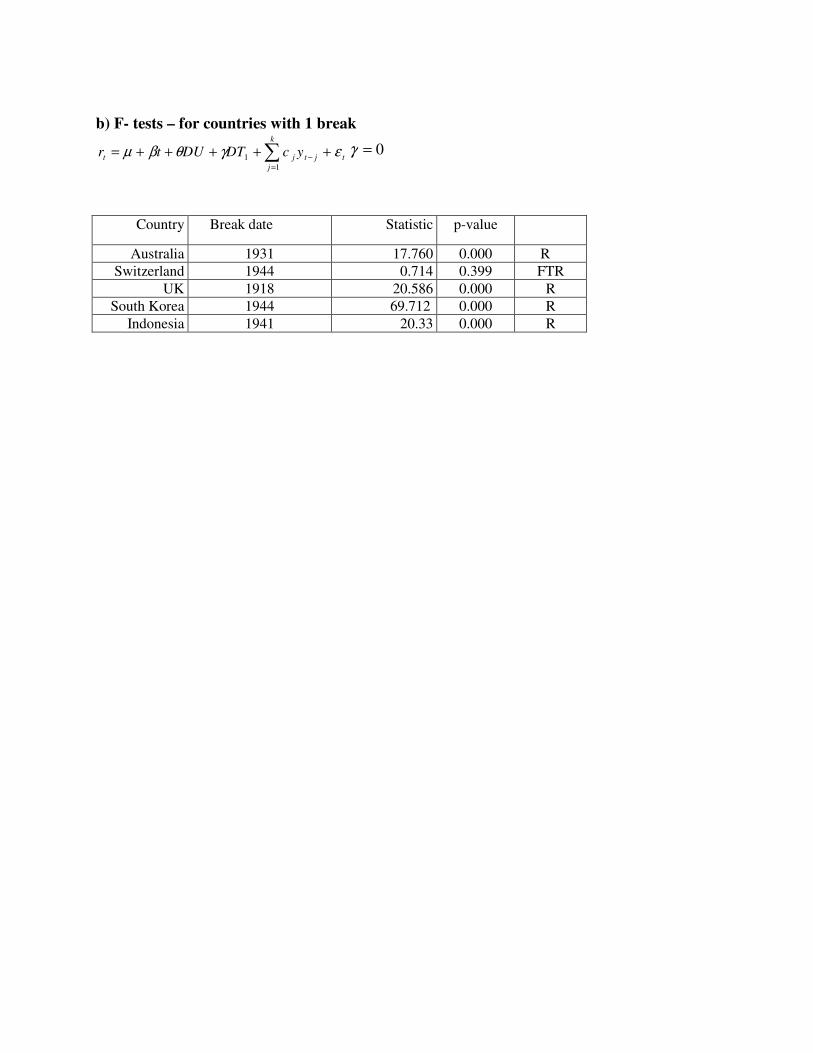
b) F- tests – for countries with 1 break

t

k

j

jtjt ycDTDUtr εγθβµ +++++= ∑=

−1

10=γ

Country Break date Statistic p-value

Australia 1931 17.760 0.000 R

Switzerland 1944 0.714 0.399 FTR

UK 1918 20.586 0.000 R

South Korea 1944 69.712 0.000 R

Indonesia 1941 20.33 0.000 R

Table 5. Prebreak (first break) and post - 1974 steady state rates of growth

Country Break dates Pre – first break

Post 1974 Ratio

Post 1974/Prefirst break

Australia 1931 0.54% 2.00% 3.70

Austria 1944, 1950 0.84% 1.99% 2.37

Belgium 1939, 1976 0.86% 1.84% 2.14

Canada 1930, 1940 1.97% 1.56% 0.79

Denmark 1939, 1969 1.62% 1.79% 1.10

France 1939, 1972 1.26% 1.59% 1.26

Germany 1944, 1950 1.30% 1.45% 1.12

Italy 1942, 1948 1.36% 1.95% 1.43

Japan 1944, 1972 1.83% 2.40% 1.31

Netherlands 1943, 1946 0.90% 1.75% 1.94

Spain 1935, 1974 0.92% 2.46% 2.67

Sweden 1916,1968 1.38% 1.48% 1.07

Switzerland 1944 1.52% 0.87% 0.57

UK 1918 1.02% 2.07% 2.03

US 1929, 1942 1.69% 2.02% 1.20

Sri Lanka 1900,1966 1.56% 3.22% 2.06

South Korea 1944 1.59% 5.92% 3.72

Taiwan 1942,1986 1.96% 5.18% 2.64

Philippine 1946,1952 1.04% 0.37% 0.36

Indonesia 1941 0.93% 3.27% 3.52

Figure 1.

West European Countries

Austria, 1870-1998

Years

1870 1882 1894 1906 1918 1930 1942 1954 1966 1978 19901.95

2.00

2.05

2.10

2.15

2.20

2.25

2.30

2.35GDP per capita

estimation

restricted

Belgium, 1870-1998

Years

1870 1882 1894 1906 1918 1930 1942 1954 1966 1978 19902.05

2.10

2.15

2.20

2.25

2.30GDP per capita

estimation

restricted

Germany, 1870-1998

Years

1870 1882 1894 1906 1918 1930 1942 1954 1966 1978 19902.00

2.05

2.10

2.15

2.20

2.25

2.30

2.35GDP per capita

estimation

restricted

FRANCE, 1870-1998

Years

1870 1882 1894 1906 1918 1930 1942 1954 1966 1978 19902.00

2.05

2.10

2.15

2.20

2.25

2.30GDP per capita

estimation

restricted

Italy, 1870-1998

Years

1870 1882 1894 1906 1918 1930 1942 1954 1966 1978 19901.95

2.00

2.05

2.10

2.15

2.20

2.25

2.30

2.35GDP per capita

estimation

restricted

Finland, 1870-1998

Years

1870 1882 1894 1906 1918 1930 1942 1954 1966 1978 19901.90

1.95

2.00

2.05

2.10

2.15

2.20

2.25

2.30

2.35GDP per capita

estimation

restricted

Denmark, 1870-1998

Years

1870 1882 1894 1906 1918 1930 1942 1954 1966 1978 19902.00

2.05

2.10

2.15

2.20

2.25

2.30

2.35GDP per capita

estimation

restricted

UK, 1870-1998

Years

1870 1882 1894 1906 1918 1930 1942 1954 1966 1978 19902.05

2.10

2.15

2.20

2.25

2.30GDP per capita

estimation

restricted

Netherlands, 1870-1998

Years

1870 1882 1894 1906 1918 1930 1942 1954 1966 1978 19902.05

2.10

2.15

2.20

2.25

2.30

2.35GDP per capita

estimation

restricted

Norway, 1870-1998

Years

1870 1882 1894 1906 1918 1930 1942 1954 1966 1978 19901.95

2.00

2.05

2.10

2.15

2.20

2.25

2.30

2.35GDP per capita

Sweden, 1870-1998

Years

1870 1882 1894 1906 1918 1930 1942 1954 1966 1978 19902.00

2.05

2.10

2.15

2.20

2.25

2.30GDP per capita

estimation

restricted

Switzerland, 1870-1998

Years

1870 1882 1894 1906 1918 1930 1942 1954 1966 1978 19902.00

2.04

2.08

2.12

2.16

2.20

2.24

2.28

2.32GDP per capita

estimation

restricted

Spain, 1870-1998

Years

1870 1882 1894 1906 1918 1930 1942 1954 1966 1978 19901.95

2.00

2.05

2.10

2.15

2.20

2.25

2.30GDP per capita

estimation

restricted

PORTUGAL, 1870-1998

Years

1870 1882 1894 1906 1918 1930 1942 1954 1966 1978 19901.90

1.95

2.00

2.05

2.10

2.15

2.20

2.25GDP per capita

Western Offshoots

United States, 1870-1998

Years

1870 1882 1894 1906 1918 1930 1942 1954 1966 1978 19902.05

2.10

2.15

2.20

2.25

2.30

2.35GDP per capita

estimation

restricted

Australia, 1870-1998

Years

1870 1882 1894 1906 1918 1930 1942 1954 1966 1978 19902.075

2.100

2.125

2.150

2.175

2.200

2.225

2.250

2.275

2.300GDP per capita

est imation

New Zealand, 1870-1998

Years

1870 1882 1894 1906 1918 1930 1942 1954 1966 1978 19902.075

2.100

2.125

2.150

2.175

2.200

2.225

2.250

2.275GDP per capita

restricted

Canada, 1870-1998

Years

1870 1882 1894 1906 1918 1930 1942 1954 1966 1978 19901.995

2.030

2.065

2.100

2.135

2.170

2.205

2.240

2.275

2.310GDP per capita

estimation

restricted

Asia

Japan, 1870-1998

Years

1870 1882 1894 1906 1918 1930 1942 1954 1966 1978 19901.85

1.90

1.95

2.00

2.05

2.10

2.15

2.20

2.25

2.30GDP per capita

estimation

restricted

South Korea, 1870-2004

Years

1911 1922 1933 1944 1955 1966 1977 1988 19996.0

6.5

7.0

7.5

8.0

8.5

9.0

9.5

10.0GDP per capita

estimation

restricted

Philippine , 1870-2004

Years

1903 1914 1925 1936 1947 1958 1969 1980 1991 20026.4

6.6

6.8

7.0

7.2

7.4

7.6

7.8

8.0G DP per capita

estimation

restricted

Sri Lanka, 1870-2004

Years

1870 1885 1900 1915 1930 1945 1960 1975 19906.25

6.50

6.75

7.00

7.25

7.50

7.75

8.00

8.25

8.50GDP per capita

est imat ion

restricted

Taiwan, 1870-2004

Years

1911 1922 1933 1944 1955 1966 1977 1988 19996.0

6.5

7.0

7.5

8.0

8.5

9.0

9.5

10.0GDP per capita

estimation

restricted

Indonesia, 1870-1998

Years

1870 1885 1900 1915 1930 1945 1960 1975 19906.00

6.25

6.50

6.75

7.00

7.25

7.50

7.75

8.00

8.25GDP per capita

estimation

restricted