tesi di laurea magistrale - unipd.ittesi.cab.unipd.it/53541/1/tesi_lm_lucchetta.pdf · corso di...
TRANSCRIPT

Universita degli Studi di Padova
DIPARTIMENTO DI FISICA E ASTRONOMIA ”GALILEO GALILEI”
Corso di Laurea in Fisica
Tesi di Laurea Magistrale
Design and optimization around 1 MeV of a Tracker for aCubeSat Mission
Candidato:
Giulio LucchettaMatricola 1106625
Relatore:
Dott. Riccardo Rando
Correlatore:
Prof. Denis Bastieri
Anno Accademico 2015-2016


Contents
Abstract 1
Introduzione 3
1 Gamma-ray astrophysics in the MeV regime 51.1 Astronomical sources . . . . . . . . . . . . . . . . . . . . . . . 5
1.1.1 Supernovae (SNe) and nucleosynthesis . . . . . . . . . 51.1.2 Gamma-Ray Bursts (GRBs) . . . . . . . . . . . . . . . 71.1.3 Active Galactic Nuclei (AGNs) . . . . . . . . . . . . . 7
1.2 Compton Scattering . . . . . . . . . . . . . . . . . . . . . . . 101.3 Compton Scattering in a real-life Instrument . . . . . . . . . . 131.4 Angular resolution for Compton events . . . . . . . . . . . . . 15
2 Compton Telescopes 172.1 Operating principle . . . . . . . . . . . . . . . . . . . . . . . . 172.2 The COMPTEL instrument . . . . . . . . . . . . . . . . . . . 182.3 COMPTEL performances . . . . . . . . . . . . . . . . . . . . 21
2.3.1 Effective Area . . . . . . . . . . . . . . . . . . . . . . . 212.3.2 Energy Responce . . . . . . . . . . . . . . . . . . . . . 222.3.3 ARM Distribution . . . . . . . . . . . . . . . . . . . . 22
2.4 Lessons learnt from COMPTEL . . . . . . . . . . . . . . . . . 232.5 General guidelines for a future Compton Telescope . . . . . . 25
3 Silicon Tracker 273.1 Properties of a tracker for Compton Telescopes . . . . . . . . 273.2 Noise in a Silicon strip detector . . . . . . . . . . . . . . . . . 29
4 Detector design and simulations 334.1 The MEGAlib software package . . . . . . . . . . . . . . . . . 334.2 Defining detector’s geometry: Starting geometry . . . . . . . . 354.3 First simulations . . . . . . . . . . . . . . . . . . . . . . . . . 37
i

ii CONTENTS
4.4 Only-calorimeter geometry . . . . . . . . . . . . . . . . . . . . 404.5 Lateral calorimeter geometry . . . . . . . . . . . . . . . . . . . 424.6 Performances under pair production . . . . . . . . . . . . . . . 45
5 Event selection and tracker optimization in the Comptonregime 495.1 Tracked events and event selection . . . . . . . . . . . . . . . 495.2 Layers number simulations . . . . . . . . . . . . . . . . . . . . 535.3 Layers thickness simulations . . . . . . . . . . . . . . . . . . . 545.4 Strip pitch simulations . . . . . . . . . . . . . . . . . . . . . . 555.5 Bit digitization simulations . . . . . . . . . . . . . . . . . . . . 565.6 Equivalent Noise Charge simulations . . . . . . . . . . . . . . 57
6 Background and sensitivity estimation 596.1 Background events . . . . . . . . . . . . . . . . . . . . . . . . 596.2 Sensitivity estimation . . . . . . . . . . . . . . . . . . . . . . . 61
7 Conclusions 65
A Quality cuts 67
B Tracker optimization plots 71
C Abbreviations and notations used 81
Ringraziamenti 83
Bibliography 85
List of Figures
1.1 Decay rates of the SN Ia model, W7, and the SN II model,W10HMM; both SNe are assumed at a distance of 10 Mpc(figures taken from [12]). . . . . . . . . . . . . . . . . . . . . . 6
1.2 Spectral energy distribution of the blazar Mrk 421 averagedover all the observations taken by different telescopes from2009 January 19, to 2009 June 1 ([4]). . . . . . . . . . . . . . . 8
1.3 Cross-section for the four dominating photon-interaction mech-anisms in Silicon ([30]). . . . . . . . . . . . . . . . . . . . . . . 10
1.4 Representation of a Compton-scattering process ([30]). . . . . 111.5 Klein-Nishina cross-section as a function of the Compton scat-
ter angle ϕ for different energies ([30]). . . . . . . . . . . . . . 111.6 Example of a polarization signal for a 100% polarized gamma-
ray beam ([30]). . . . . . . . . . . . . . . . . . . . . . . . . . . 121.7 Reconstruction of the Compton gamma-ray direction in the
case of incomplete measurements (image taken from [30]). . . 131.8 Energy of the recoil electron vs. energy of the scattered gamma-
ray for a fixed total scatter angle θ ([30]). . . . . . . . . . . . . 141.9 Compton cross section for unbound and bound Compton scat-
tering in Silicon, as a function of incident gamma-ray energy(left), and Compton scatter angle at 100 keV (right). Thepictures are taken from [30] . . . . . . . . . . . . . . . . . . . 15
2.1 Comparison of two different Compton telescopes: a "COMP-TEL type" instrument and a "modern type" instrument witha tracker (picture taken from https://www.med.physik.uni-muenchen.de/research/new-detectors/index.html). . . . . . . . 18
2.2 Schematic diagram of COMPTEL Instrument, as illustratedin [15]. . . . . . . . . . . . . . . . . . . . . . . . . . . . . . . . 19
2.3 COMPTEL effective area as a funtion of the incident photonenergy (picture taken from [18]). . . . . . . . . . . . . . . . . . 21
iii
iv LIST OF FIGURES
2.4 COMPTEL energy responce to a 4.430 MeV (left) and a12.143 MeV (right) monoenergetic point source at normalincidence (pictures taken from [18]). . . . . . . . . . . . . . . . 22
2.5 COMPTEL ARM distribution for a 4.430 MeV (left) anda 12.143 MeV (right) monoenergetic point source at normalincidence (pictures taken from [18]). . . . . . . . . . . . . . . . 23
2.6 Illustration of the point source continuum sensitivity for differ-ent X and Gamma-ray Telescopes, as reported in [21].COMP-TEL sensitivity is estimated for an observation time of 106 s. . 23
2.7 Background environment for an equatorial 550 km LEO orbitcomputed in the ASTROGAM proposal ([25]). . . . . . . . . . 24
2.8 Schematic diagram for future Compton Telescopes, taken from[25] and [9]. . . . . . . . . . . . . . . . . . . . . . . . . . . . . 26
3.1 Angular resolution as a function of the atomic number Z,assuming ideal detector properties ([30]). . . . . . . . . . . . . 28
3.2 Detector front-end circuit (picture taken from [23]). . . . . . . 303.3 Equivalent noise charge as a function of the CR-RC peaking
time. . . . . . . . . . . . . . . . . . . . . . . . . . . . . . . . . 31
4.1 Schematic diagram of the telescope starting geometry. . . . . . 354.2 Energy and ARM spectra for the 100 keV simulation with the
starting geometry. . . . . . . . . . . . . . . . . . . . . . . . . . 374.3 Energy and ARM spectra for the 333 keV simulation with the
starting geometry. . . . . . . . . . . . . . . . . . . . . . . . . . 384.4 Energy and ARM spectra for the 2 MeV simulation with the
starting geometry. . . . . . . . . . . . . . . . . . . . . . . . . . 384.5 Illustration of the concept of the surrounding sphere (picture
taken from Cosima manual). . . . . . . . . . . . . . . . . . . . 394.6 Comparison of the effective areas estimated from only-calorimeter
configuration and starting configuration. . . . . . . . . . . . . . 414.7 Comparison of the ARM spectrum from only calorimeter config-
uration (left) and starting configuration (right), for a 333 keVsimulation. . . . . . . . . . . . . . . . . . . . . . . . . . . . . . 41
4.8 Comparison of the ARM spectrum from only calorimeter con-figuration (left) and starting configuration (right), for a 1 MeVsimulation. . . . . . . . . . . . . . . . . . . . . . . . . . . . . . 42
4.9 Comparison of the energy spectrum from only calorimeterconfiguration (left) and starting configuration (right), for a1 MeV simulation. . . . . . . . . . . . . . . . . . . . . . . . . . 42
4.10 Events distribution in the x-y plane for a 333 keV simulation. . 43

LIST OF FIGURES v
4.11 Schematic diagram of the telescope final geometry. . . . . . . . 434.12 Effective area estimated from simulations with and without
lateral calorimeters. . . . . . . . . . . . . . . . . . . . . . . . . 444.13 Energy and PSF spectra under pair detection for the 2 MeV
simulation. . . . . . . . . . . . . . . . . . . . . . . . . . . . . . 454.14 Energy and PSF spectra under pair detection for the 5 MeV
simulation. . . . . . . . . . . . . . . . . . . . . . . . . . . . . . 464.15 Comparison of the effective area for Compton scattering and
pair production. . . . . . . . . . . . . . . . . . . . . . . . . . . 464.16 PSF containment intervals before and after quality cuts. . . . 47
5.1 Energy and ARM spectra for tracked and not tracked eventsin a 1 MeV simulation. . . . . . . . . . . . . . . . . . . . . . . 49
5.2 SPD distribution for a 1 MeV simulation. . . . . . . . . . . . . 505.3 Parameters estimated for the standard configuration. . . . . . 515.4 Comparison of the energy resolutions for the simulations with
different number of layers. . . . . . . . . . . . . . . . . . . . . 535.5 Parameters comparison for the simulations with different thick-
ness for the layers (tracked + bottom calorimeter events). . . . 545.6 Parameters comparison for the simulations with different thick-
ness for the layers (tracked + lateral calorimeter events). . . . 545.7 Comparison of the energy resolutions for the simulations with
different strip pitch. . . . . . . . . . . . . . . . . . . . . . . . . 555.8 Comparison of the ARM FWHM for simulations with different
strip pitch. . . . . . . . . . . . . . . . . . . . . . . . . . . . . . 565.9 Comparison of the energy resolutions for the bit digitization
simulations. . . . . . . . . . . . . . . . . . . . . . . . . . . . . 565.10 Comparison of the energy resolutions for the different noise
simulations. . . . . . . . . . . . . . . . . . . . . . . . . . . . . 57
6.1 Albedo and EGB simulated counts spectra (log scale). . . . . . 606.2 Effictive area for different energies and zenit angles for tracked
plus lateral calorimeter events. . . . . . . . . . . . . . . . . . . 61
A.1 ARM spectrum for a 2 MeV simulation with and without cuts. 68A.2 Example of some spectra with and without quality cuts. . . . 68A.3 Results after quality cuts. . . . . . . . . . . . . . . . . . . . . 69
B.1 Parameters estimated for the configuration with 20 layers. . . 71B.2 Parameters estimated for the configuration with 25 layers. . . 72B.3 Parameters estimated for the configuration with 400 µm layer
thickness. . . . . . . . . . . . . . . . . . . . . . . . . . . . . . 73

vi LIST OF FIGURES
B.4 Parameters estimated for the configuration with 600 µm layerthickness. . . . . . . . . . . . . . . . . . . . . . . . . . . . . . 74
B.5 Parameters estimated for the configuration with a strip pitchof 50 µm. . . . . . . . . . . . . . . . . . . . . . . . . . . . . . 75
B.6 Parameters estimated for the configuration with a strip pitchof 300 µm. . . . . . . . . . . . . . . . . . . . . . . . . . . . . . 76
B.7 Parameters estimated for the configuration with a 8 bit digiti-zation. . . . . . . . . . . . . . . . . . . . . . . . . . . . . . . . 77
B.8 Parameters estimated for the configuration with a 12 bit digi-tization. . . . . . . . . . . . . . . . . . . . . . . . . . . . . . . 78
B.9 Parameters estimated for the configuration with a 600 e− ENC. 79B.10 Parameters estimated for the configuration with a 2400 e− ENC. 80

List of Tables
3.1 Parameters used for the equivalent noise charge estimation. . . 31
4.1 Tracker main parameters for the starting geometry. . . . . . . 364.2 Calorimeter main parameters for the starting geometry. . . . . 374.3 Telescope performances for the starting geometry. . . . . . . . 404.4 Telescope performances for the lateral calorimeter geometry. . 44
5.1 Parameters considered for the silicon tracker optimization.In bold are reported the parameters used in the standardconfiguration. . . . . . . . . . . . . . . . . . . . . . . . . . . . 52
6.1 Parameters used for the sensitivity calculation for tracked plusbottom calorimeter events. . . . . . . . . . . . . . . . . . . . . 63
6.2 Parameters used for the sensitivity calculation for tracked pluslateral calorimeter events. . . . . . . . . . . . . . . . . . . . . 63
6.3 Parameters used for the sensitivity calculation for not trackedplus bottom calorimeter events. . . . . . . . . . . . . . . . . . 63
6.4 Sensitivity expressed in ph cm−2 s−1 for different events classes. 64
vii

viii

Abstract
Gamma-ray astrophysics is quite a young field, especially in comparison to thelong history of optical observations or even radio-astronomy. Starting with thefirst observations of telescopes like OSO3 (1967-1969) and SAS2 (1972-1973),in the last two decades many space observatories obtained considerable results:FERMI-LAT (2008-), in the energy range from 20 MeV to 300 GeV, AGILE(2007-), in the energy range from 30 MeV to 50 GeV, COMPTEL (1991-2000),in the energy range from 1 to 30 MeV, and INTEGRAL-IBIS (2002-), in theenergy range from 15 keV to 10 MeV, only to name but a few gamma-rayobservatories.At present, the worse sensitivity occurs in the range 1− 10 MeV, where thedominant interaction mechanism of gamma rays with matter is Comptonscattering. The scientific interest towards this area of the electromagneticspectrum is actually remarkable. In fact, the MeV regime can provide uniqueinformations about cosmic accelerators, in particular thanks to the detailedstudy of several emission lines. New data and informations in this range areessential to understand the physical processes powering several cosmic sourceslike pulsars, supernovae and active galactic nuclei.For these reasons the next generation of space observatories for gamma-rayastrophysics will focus on the energy range around 1 MeV.
The best instrument to date in this range, COMPTEL onboard CGRO,flew in the 1990’s but with a technology dating to a decade earlier. Theoperating principle of the detector was based on Compton interaction in oneof a series of liquid scintillators, and the consecutive absorption in a secondplane of NaI scintillators at the distance of 150 cm.Given the huge leap in technology that occurred since, such as the devel-opment of semiconductor detectors and the experience gathered with othergamma-ray observatories like the FERMI-LAT, the performances of a futureCompton telescope is expected to improve at least by an order of magnitudewith respect to COMPTEL. However, several issues affect this optimisticpicture of the situation: the external gamma-ray background produced by the
1
2 LIST OF TABLES
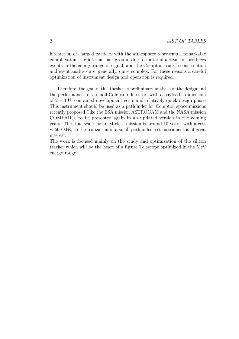
interaction of charged particles with the atmosphere represents a remarkablecomplication, the internal background due to material activation producesevents in the energy range of signal, and the Compton track reconstructionand event analysis are, generally, quite complex. For these reasons a carefuloptimization of instrument design and operation is required.
Therefore, the goal of this thesis is a preliminary analysis of the design andthe performances of a small Compton detector, with a payload’s dimensionof 2 − 3 U, contained development costs and relatively quick design phase.This instrument should be used as a pathfinder for Compton space missionsrecently proposed (like the ESA mission ASTROGAM and the NASA missionCOMPAIR), to be presented again in an updated version in the comingyears. The time scale for an M-class mission is around 10 years, with a cost∼ 500 Me, so the realization of a small pathfinder test instrument is of greatinterest.The work is focused mainly on the study and optimization of the silicontracker which will be the heart of a future Telescope optimized in the MeVenergy range.

Introduzione
L’astrofisica delle alte energie è un campo relativamente giovane della fisica,specialmente se confrontato con la lunga storia delle osservazioni nell’ottico,o con la radio-astronomia. Partendo dalle prime osservazioni di telescopicome OSO3 (1967-1969) e SAS2 (1972-1973), negli ultimi venti anni numerosiosservatori spaziali hanno ottenuto risultati notevoli: FERMI-LAT (2008-),nel range energetico compreso tra 20 MeV e 300 GeV, AGILE (2007-), nelrange compreso tra 30 MeV e 50 GeV, COMPTEL (1991-2000), nel rangecompreso tra 1 e 30 MeV, ed INTEGRAL-IBIS (2002-), nel range compresotra 15 keV e 10 MeV, solo per citarne alcuni.Attualmente la sensitività peggiore è proprio nella finestra 1−10 MeV, dove ilmeccanismo principale di interazione dei fotoni con la materia è rappresentatodallo scattering Compton. Tuttavia l’interesse scientifico rivolto a questaregione dello spettro elettromagnetico è notevole. Infatti, nel regime del MeV,si possono ottenere prezione informazioni che riguardano gli acceletatori cos-mici, in particolare grazie allo studio dettagliato di diverse linee di emissione.Nuovi dati ed informazioni in questo range energetico sono quindi essenzialiper comprendere i processi fisici che regolano diverse sorgenti cosmiche comele pulsar, le supernove e i nuclei galattici attivi.
Lo strumento che in passato ha coperto il range intorno ad 1 MeV, COMP-TEL, ha iniziato la presa dati negli anni ’90 ma fu costruito con una tecnologiasviluppata negli anni ’80. Il principio di funzionamento del rivelatore si basavasull’interazione Compton in un primo modulo di scintillatori liquidi, e il suc-cessivo assorbimento da parte di un secondo modulo di scintillatori allo Iodurodi Sodio, posti alla distanza di 150 cm rispetto ai primi.Considerati i grandi passi in avanti compiuti da allora dal punto di vistatecnologico, come lo sviluppo dei rivelatori a semiconduttore, e l’esperienzaaccumulata attraverso altre missioni spaziali come il FERMI-LAT, è possibilepensare alla realizzazione di un nuovo satellite Compton con delle prestazionimigliori rispetto a quelle di COMPTEL di almeno un ordine di grandezza.Tuttavia, diversi problemi complicano questo quadro ottimistico della situ-
3

4 LIST OF TABLES
azione: il background esterno di raggi gamma prodotti dall’interazione diparticelle cariche con l’atmosfera rappresenta un’enorme fonte di disturbo,il background interno dovuto all’attivazione di materiale passivo produceeventi nel range energetico in esame, e la ricostruzione e l’analisi degli eventiCompton è, generalmente, piuttosto complessa. Per tutti questi motivi ènecessaria un’accurata progettazione del satellite e un’attenta ottimizzazionedella strumentazione e della procedura di analisi dati.
Pertanto, lo scopo di questa tesi consiste nell’analisi preliminare dellaprogettazione e delle prestazioni di un piccolo satellite Compton, con unpayload delle dimensioni di circa 2− 3 U, dai costi contenuti e progettabilein tempi relativamente brevi. Questo telescopio potrà essere utilizzato comestrumento di test in vista di missioni presentate di recente (come la missioneESA ASTROGAM, e la missione NASA COMPAIR) e che saranno ripropostein versione aggiornata nei prossimi anni. Poiché il time scale per una missionedi classe M è di circa 10 anni, con un costo ∼ 500 Me, la realizzazione di unapiccola sonda pathfinder è di grande interesse.In particolare il lavoro svolto si è focalizzato principalmente sullo studio esull’ottimizzazione del tracciatore al silicio, il quale, come vedremo, rappre-senta l’elemento fondamentale per un futuro telescopio ottimizzato nel rangeenergetico attorno al MeV.

Chapter 1
Gamma-ray astrophysics in theMeV regime
1.1 Astronomical sourcesGamma-ray astronomy in the MeV regime, from a few hundred keV to severaltens of MeV, can provide unique information about the universe. The highpenetration power of the gamma rays enables studies of highly obscuredsources, and nuclear lines carry information about origin and distributionof individual isotopes in the cosmos, and the underlying processes poweringseveral cosmic sources like supernovae, novae, pulsars etc.It is not the purpose of this thesis to give a complete and detailed descriptionof all these astronomical sources; in fact in this section are presented onlysome fundamentals science objectives for a future Compton Telescope. Forfurther information see, for example, [25] and [14].
1.1.1 Supernovae (SNe) and nucleosynthesisOne of the most challenging questions in gamma-ray astronomy is related totype Ia Supernovae.Supernovae are the brilliant death of a star; these astronomical events can bedue to the thermonuclear explosion of a CO white dwarf (SNe Ia) or to the core-collapse of a massive star (SNe II/Ib/Ic). Supernovae have synthesized mostof the elements heavier than He, and their light curve is powered, mainly, bythe decay 56Ni→56 Co (t1/2 = 6.1 d, with a 812 keV line) and 56Co→56 Fe(t1/2 = 77 d, with a line at 847 keV ). A much smaller contribution is given by57Co, 44Ti, 22Na and 60Co, as illustrated in Figure 2.8. Evident in the figureis the cascade from the early-time dominance of short-lived radioactivitiesto the later dominance of long-lived radioactivities. Assuming that a large
5

6CHAPTER 1. GAMMA-RAY ASTROPHYSICS IN THE MEV REGIME
fraction of these photons escape, short-lived radioactivities give rise to intense,but brief emission, while long-lived radioactivities give rise to faint, butpersistent emission. Moreover, type II Supernovae produce less 56Ni thantype Ia Supernovae (the difference of a factor of eight can not be properlyidentified, since the large scale of the figure), so prompt emission is far fainterin SNe II than SNe Ia.Initially, the SN density is so large that all X and gamma-ray photons arescattered, but, as the SN expands, the ejecta thins and photons begin toescape. Therefore, the prompt X and gamma-ray line flux from a SN dependsupon ejecta mass and kinematics, making the evolution of the fluxes of thevarious gamma-ray lines a probe of the SN ejecta. In fact, the measurementof the intensity of these lines provides a direct and precise determination ofthe 56Co mass, which is the main parameter that determines the evolution ofoptical light curve and relationship between the intensity of the peak and theslope of the post peak.
(a) Type Ia Supernova. (b) Type II Supernova.
Figure 1.1: Decay rates of the SN Ia model, W7, and the SN II model,W10HMM; both SNe are assumed at a distance of 10 Mpc (figures taken from[12]).
Although SNe Ia are used as standard candles to measure cosmologicaldistances, many questions about these explosions remain unanswered. Firstlywe do not yet know which are the progenitor systems: it is almost certainlythat these processes occur in binary systems, but the nature of the compan-ions, whether normal stars or white dwarfs, is still unknown. Moreover, wedo not clear understand the propagation processes and several competingmodels of explosion mechanisms exist: for example, we do not know if theburning front propagates subsonically or supersonically, or a mixture of thetwo, and to what extent instabilities break spherical symmetry.The study of gamma-ray line emission in the MeV regime is an excellent
1.1. ASTRONOMICAL SOURCES 7
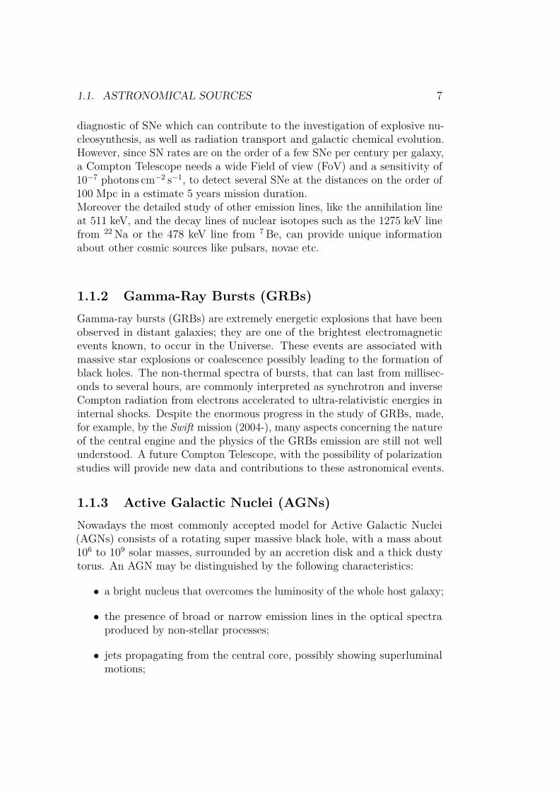
diagnostic of SNe which can contribute to the investigation of explosive nu-cleosynthesis, as well as radiation transport and galactic chemical evolution.However, since SN rates are on the order of a few SNe per century per galaxy,a Compton Telescope needs a wide Field of view (FoV) and a sensitivity of10−7 photons cm−2 s−1, to detect several SNe at the distances on the order of100 Mpc in a estimate 5 years mission duration.Moreover the detailed study of other emission lines, like the annihilation lineat 511 keV, and the decay lines of nuclear isotopes such as the 1275 keV linefrom 22 Na or the 478 keV line from 7 Be, can provide unique informationabout other cosmic sources like pulsars, novae etc.
1.1.2 Gamma-Ray Bursts (GRBs)Gamma-ray bursts (GRBs) are extremely energetic explosions that have beenobserved in distant galaxies; they are one of the brightest electromagneticevents known, to occur in the Universe. These events are associated withmassive star explosions or coalescence possibly leading to the formation ofblack holes. The non-thermal spectra of bursts, that can last from millisec-onds to several hours, are commonly interpreted as synchrotron and inverseCompton radiation from electrons accelerated to ultra-relativistic energies ininternal shocks. Despite the enormous progress in the study of GRBs, made,for example, by the Swift mission (2004-), many aspects concerning the natureof the central engine and the physics of the GRBs emission are still not wellunderstood. A future Compton Telescope, with the possibility of polarizationstudies will provide new data and contributions to these astronomical events.
1.1.3 Active Galactic Nuclei (AGNs)Nowadays the most commonly accepted model for Active Galactic Nuclei(AGNs) consists of a rotating super massive black hole, with a mass about106 to 109 solar masses, surrounded by an accretion disk and a thick dustytorus. An AGN may be distinguished by the following characteristics:
• a bright nucleus that overcomes the luminosity of the whole host galaxy;
• the presence of broad or narrow emission lines in the optical spectraproduced by non-stellar processes;
• jets propagating from the central core, possibly showing superluminalmotions;
8CHAPTER 1. GAMMA-RAY ASTROPHYSICS IN THE MEV REGIME
• continuum non-thermal emission in several wavelength, from radio togamma-ray band;
• strong variability of the electromagnetic emission, on time scales fromhours to years.
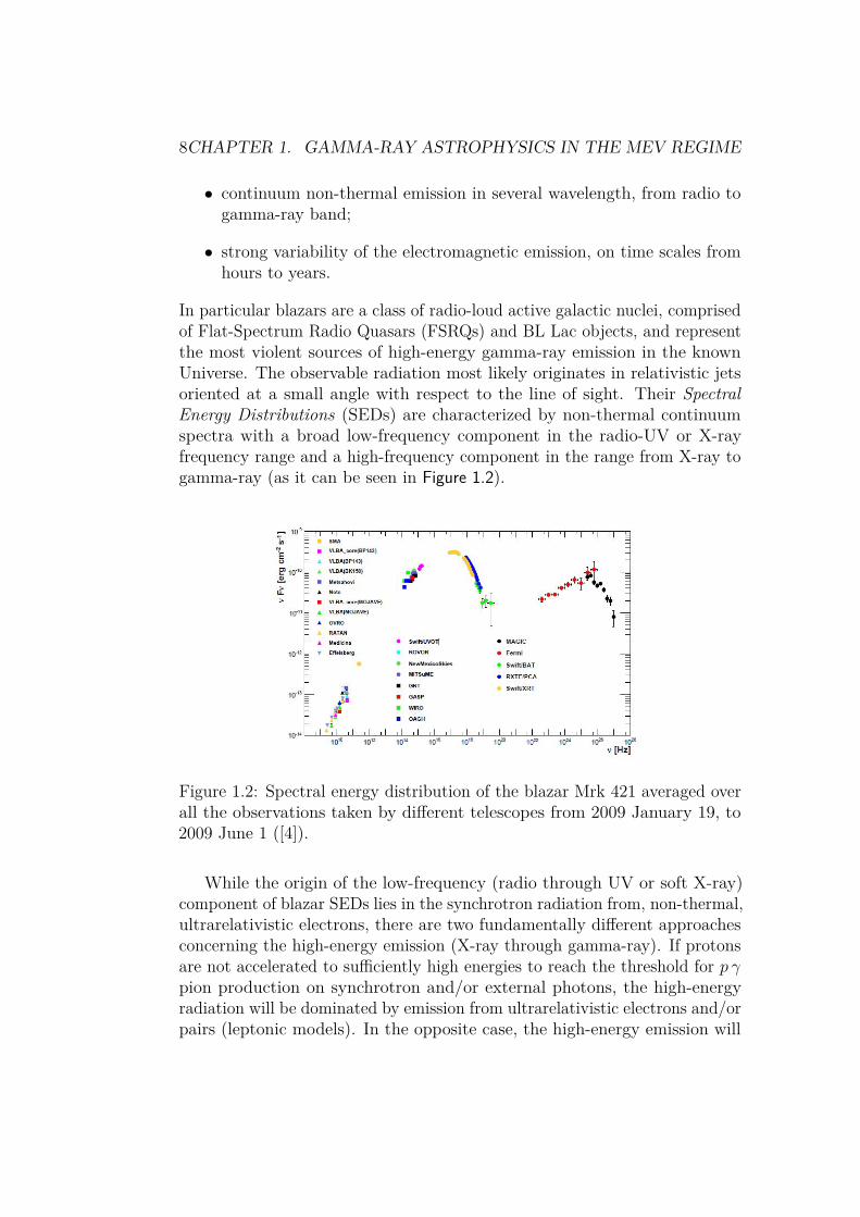
In particular blazars are a class of radio-loud active galactic nuclei, comprisedof Flat-Spectrum Radio Quasars (FSRQs) and BL Lac objects, and representthe most violent sources of high-energy gamma-ray emission in the knownUniverse. The observable radiation most likely originates in relativistic jetsoriented at a small angle with respect to the line of sight. Their SpectralEnergy Distributions (SEDs) are characterized by non-thermal continuumspectra with a broad low-frequency component in the radio-UV or X-rayfrequency range and a high-frequency component in the range from X-ray togamma-ray (as it can be seen in Figure 1.2).
Figure 1.2: Spectral energy distribution of the blazar Mrk 421 averaged overall the observations taken by different telescopes from 2009 January 19, to2009 June 1 ([4]).
While the origin of the low-frequency (radio through UV or soft X-ray)component of blazar SEDs lies in the synchrotron radiation from, non-thermal,ultrarelativistic electrons, there are two fundamentally different approachesconcerning the high-energy emission (X-ray through gamma-ray). If protonsare not accelerated to sufficiently high energies to reach the threshold for p γpion production on synchrotron and/or external photons, the high-energyradiation will be dominated by emission from ultrarelativistic electrons and/orpairs (leptonic models). In the opposite case, the high-energy emission will

1.1. ASTRONOMICAL SOURCES 9
be dominated by cascades initiated by p γ pair and pion production as wellas proton, π±, and µ± synchrotron radiation (hadronic models).
• Leptonic blazar models. In leptonic models, the radiative outputthroughout the electromagnetic spectrum is assumed to be dominated byleptons (electrons and positrons). Any protons that are likely present inthe outflow, are not accelerated to sufficiently high energies to contributesignificantly to the radiative output. The high-energy emission is thenmost plausibly explained by Compton scattering of low-energy photonsby the same electrons producing the synchrotron emission at lowerfrequencies. Possible target photon fields are the synchrotron photonsproduced within the jet (the synchrotron self-Compton (SSC) process)or external photons (the external Compton process). Leptonic models,which require the specification of a rather large number of parameters,have met great success in modeling the spectral energy distribution(SEDs) of a large class of blazars. However, the very fast variability ofsome blazars, poses several problems in the modeling of some sourcesas, for example, W Comae and 3C 66A (Böettcher et al., 2013 ).
• Hadronic blazar models. In hadronic models, both primary electronsand protons are accelerated to ultrarelativistic energies, with protonsexceeding the threshold for p γ pion production. The acceleration ofprotons to the necessary ultrarelativistic energies requires high magneticfields of at least several tens of Gauss. While the low-frequency emissionis still dominated by synchrotron emission from primary electrons, thehigh-energy emission is dominated by proton synchrotron emission, π0
decay photons, and synchrotron and Compton emission from secondarydecay products of charged pions. Hadronic modeling seems problematicin the case of some AGN like 3C 273 and 3C 279 (Böettcher et al.,2013 ).
• Hybrid blazar models. The leptonic and hadronic models discussedabove are certainly only to be regarded as extreme idealizations of ablazar jet. Realistically, both types of processes should be consideredin modeling blazar emission. Nevertheless, for the majority of blazardetected nowadays, we are not able to determine how much is hadronicemission and how much is leptonic emission.
AGNs detection in the energy range around 1 MeV, a widely unexploredregion in the electromagnetic spectrum, as it can be seen Figure 1.2 1, can
1roughly 1 MeV corresponds to 1022 Hz

10CHAPTER 1. GAMMA-RAY ASTROPHYSICS IN THE MEV REGIME
provide unique informations in this scenario, determining which component(hadronic or leptonic) is dominant for a given energy in the considered AGN.
1.2 Compton ScatteringCompton scattering, discovered by Arthur Holly Compton in 1922, is theelastic scattering of a photon by an electron. Compton cross-section dependson the atomic number Z of the scatter material; however Compton scatteringis the dominant photon-interaction process between ∼ 200 keV and ∼ 10 MeV,for the majority of materials (Figure 1.3).
Figure 1.3: Cross-section for the four dominating photon-interaction mecha-nisms in Silicon ([30]).
The Compton scattering process can be described in terms of energy andmomentum conservation of photon and electron:
Ei + Ei,e = Eg + Ee (1.1)
~pi + ~pi,e = ~pg + ~pe (1.2)In general, the initial energy Ei,e and momentum ~pi,e of the bound electronare unknown. Assuming that the electron is at rest, the previous equationsare modified as follow:
Ei + E0 = Eg + Ee (1.3)~pi = ~pg + ~pe (1.4)
where E0 = mec2 is the rest energy of the electron.
From these, the following relation between energies and Compton scatterangle can be derived:
cosϕ = 1− E0
Eg+ E0
Eg + Ee(1.5)
1.2. COMPTON SCATTERING 11
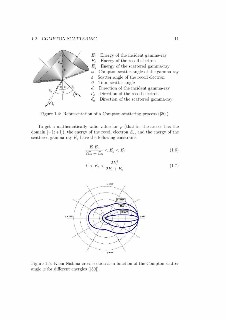
Ei Energy of the incident gamma-rayEe Energy of the recoil electronEg Energy of the scattered gamma-rayϕ Compton scatter angle of the gamma-rayε Scatter angle of the recoil electronϑ Total scatter angle~ei Direction of the incident gamma-ray~ee Direction of the recoil electron~eg Direction of the scattered gamma-ray
Figure 1.4: Representation of a Compton-scattering process ([30]).
To get a mathematically valid value for ϕ (that is, the arccos has thedomain [−1; +1]), the energy of the recoil electron Ee, and the energy of thescattered gamma ray Eg have the following constrains:
E0Ei2Ei + E0
< Eg < Ei (1.6)
0 < Ee <2E2
i
2Ei + E0(1.7)
Figure 1.5: Klein-Nishina cross-section as a function of the Compton scatterangle ϕ for different energies ([30]).
12CHAPTER 1. GAMMA-RAY ASTROPHYSICS IN THE MEV REGIME
The differential Compton cross-section for unpolarized photons scatteringof unbound electrons was derived by Klein and Nishina in 1929:(
dσ
dΩ
)C,unbound,unpol
= r2e
2
(EgEi
)2(EgEi
+ EiEg− sin2 ϕ
)(1.8)
with re classical electron radius.The forward scattering is favored at higher energies since the average Comptonscatter angle is smaller for higher energies, as represented in Figure 1.5. How-ever the Klein-Nishina cross-section constitutes only an approximation, sincethe electron is assumed not to be bound to an atom and therefore to be at rest.
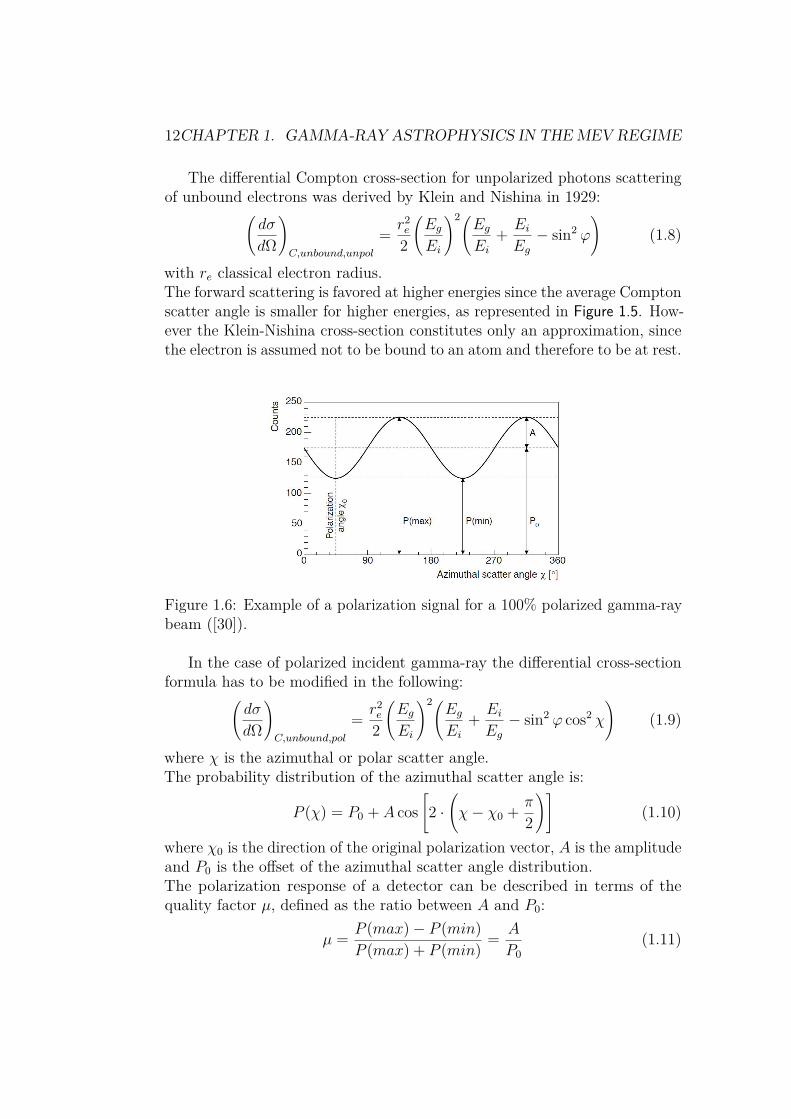
Figure 1.6: Example of a polarization signal for a 100% polarized gamma-raybeam ([30]).
In the case of polarized incident gamma-ray the differential cross-sectionformula has to be modified in the following:(
dσ
dΩ
)C,unbound,pol
= r2e
2
(EgEi
)2(EgEi
+ EiEg− sin2 ϕ cos2 χ
)(1.9)
where χ is the azimuthal or polar scatter angle.The probability distribution of the azimuthal scatter angle is:
P (χ) = P0 + A cos[2 ·(χ− χ0 + π
2
)](1.10)
where χ0 is the direction of the original polarization vector, A is the amplitudeand P0 is the offset of the azimuthal scatter angle distribution.The polarization response of a detector can be described in terms of thequality factor µ, defined as the ratio between A and P0:
µ = P (max)− P (min)P (max) + P (min) = A
P0(1.11)

1.3. COMPTON SCATTERING IN A REAL-LIFE INSTRUMENT 13
1.3 Compton Scattering in a real-life Instru-ment
In the previous section ideal Compton Scattering processes have been studied.However, in any real-life telescope, several additional aspects have to be takeninto consideration.For example if the energies of the recoil electron Ee and the scattered photonEg, as well as their directions ~ee and ~eg, are determined with high accuracy,the origin of the photon can be calculated. However, in a real detector thesefour parameters may not be all measured (or only measured with a largeerror): in this case it is still possible to constrain the origin of the incidentphoton.If the Compton scatter angle is well know, but it is not possible to measurethe electron scatter angle, the incident direction of the detected gamma-raycan be restricted to a cone whose opening angle is the Compton scatterangle ϕ. Otherwise, if the electron scatter angle can be computed, but noinformation about the photon scatter angle is present, the incident directionof the detected gamma-ray can be restricted to a cone with an opening angleε.If no energies are measured or both energies only incompletely, and the elec-tron and the photon scatter directions are well known, photon’s origin canpartly be retrieved, determining a minimum and maximum possible Comptonscatter angle (1.7).
Figure 1.7: Reconstruction of the Compton gamma-ray direction in the caseof incomplete measurements (image taken from [30]).

14CHAPTER 1. GAMMA-RAY ASTROPHYSICS IN THE MEV REGIME
As it can be seen in Figure 1.8, ϕmin and ϕmax can be calculated only forsome values of the measured gamma-ray and electron energy. If Emeas
g >E0
1−cosϑ and Emease > 2E0
tan2 ϑ, and both values are below/left of the curve, it is
possible to determine both ϕmin and ϕmax. Otherwise, if Emeasg < E0
1−cosϑ thenno limit on ϕmax can be determined, while if Emeas
e < 2E0tan2 ϑ
then no limit onϕmin can be given.
Figure 1.8: Energy of the recoil electron vs. energy of the scattered gamma-rayfor a fixed total scatter angle θ ([30]).
The second fundamental aspect to take into account in a real-life detectorsystem, is the fact that electrons are neither free nor at rest, but bound to anucleus. The unknown momentum of the electron within its atomic energyshell leads to a “Doppler broadening” of the relative energies of the electronand scattered photon, limiting the accuracy with which the incident photondirection can be reconstructed.To describe this effect, a more sophisticated Compton cross section than theKlein-Nishina equation is required. A suitable expression, that takes intoaccount the momentum distribution of the bound electrons, has been derivedby Ribberfors (1975):(
dσ
dΩ
)C,bound,i
=(dσ
dΩ
)C,unbound
SIi (Ei, ϕ, Z) (1.12)
Where Z is the atomic number of the scattering material an SIi is called theincoherent scattering function of the i-th shell electrons in the momentumapproximation. The expression for SIi has been calculated by Ritterfors andBerggren (1982).

1.4. ANGULAR RESOLUTION FOR COMPTON EVENTS 15
Figure 1.9: Compton cross section for unbound and bound Compton scatteringin Silicon, as a function of incident gamma-ray energy (left), and Comptonscatter angle at 100 keV (right). The pictures are taken from [30]
The differences between Ribberfors and Klein-Nishina cross sections areillustrated in Figure 1.9. Especially at lower energies, photons have a slightlyhigher probability to scatter than predicted by the Klein-Nishina equation.Moreover, also the scatter angle distribution changes: in the case of boundelectrons small and large scatter angles are suppressed, while the scatterprobability increases in the range between ∼ 40 and ∼ 130.
1.4 Angular resolution for Compton eventsFor Compton reconstructed events in a real-life telescope the angular resolutioncan be describe in terms of two different quantities: the Angular ResolutionMeasure or ARM, and the Scatter Plane Deviation or SPD.The ARM is defined as the difference between the computed scatter angle ϕ,and the true scatter angle ϕgeo:
ARM = ϕ− ϕgeo (1.13)
In the ideal case with no measurement errors, ARM will be zero. Howeverin a real-life instrument, energies and locations are measured with a certainerror, producing a finite width in the ARM measurement distributed aboutzero. Therefore the width of the ARM distribution is a measure of theuncertainty in the opening angle of the Compton cone for each reconstructedevent.Instead, the SPD represents the angle between the true scatter plane describedby the direction of the incident photon ~ei, and the direction of the scatteredphoton ~eg, and the measured one spanned by ~eg and ~ee (direction of the recoilelectron), assuming that ~eg has been measured correctly:
SPD = arccos((~eg × ~ei) (~eg × ~ee)) (1.14)

16CHAPTER 1. GAMMA-RAY ASTROPHYSICS IN THE MEV REGIME
Thus the SPD is relevant only if a measure of ~ee exist, that is only for trackedevents. More intuitively the scatter plane deviation describe the length of theCompton arcs (see, for example, Figure 2.1).

Chapter 2
Compton Telescopes
2.1 Operating principle
The key objective for a Compton Telescope is to determine the direction ofmotion of the scattered gamma-ray and/or the recoil electron. As illustratedin 2.1, two different types of instrument can fulfill this scope.In the first type telescopes ("COMPTEL type" telescopes) we have two detec-tor systems: a low-Z scatterer and a high-Z absorber. In the low-Z detectorthe initial Compton interaction takes place. In the high-Z detector the scat-tered gamma-ray is absorbed and measured. The two detectors are wellseparated, so that the time-of-flight of the scattered photon between the twodetectors can be measured. Thus top-to-bottom events can be distinguishedfrom bottom-to-top events. With a COMPTEL type instrument it is notpossible to measure the direction of the recoil electron, so an ambiguity in thereconstruction of the origin of original photon emerges: the origin can onlybe reconstructed to a cone. This ambiguity has to be resolved by measuringseveral photons from the source and by image reconstruction.A second group of detectors is capable of measuring the direction of the recoilelectron by tracking it. This enables the determination of the direction ofmotion of the scattered photon and allows to resolve the origin of the photonmuch more accurately: the Compton cone is reduced to a segment of the cone,whose length depends on the measurement accuracy of the recoil electron."Modern type" Compton telescopes with a tracker, have the advantage thatonly fewer photons are needed to recover the position of sources, dependingon background conditions and quality of the events. They are also inherentlysensitive to polarization. However for all those advantages a price must bepaid: the original photon is measured via several individual measurementsat different interaction positions. Each of these introduces measurement
17

18 CHAPTER 2. COMPTON TELESCOPES
errors which are propagated into the recovery of the origin and energy ofthe photon. In addition, the complexity of the measurement process requiresnon-trivial techniques to find the direction of motion and origin of the photons.
Figure 2.1: Comparison of two different Compton telescopes: a "COMP-TEL type" instrument and a "modern type" instrument with a tracker (pic-ture taken from https://www.med.physik.uni-muenchen.de/research/new-detectors/index.html).
2.2 The COMPTEL instrumentThe Compton Gamma-Ray Observatory (CGRO), launched in April 1991,performed the first full-sky survey in gamma rays. With four differentinstruments, CGRO, orbiting the Earth at nominal height of 450 km, operatedover a wide range of photon energies from about 20 keV to 30 GeV:
• the Energetic Gamma-Ray Telescope (EGRET): a spark chamber in-strument for imaging of the energy range 20 MeV− 30 GeV;
• the Imaging Compton Telescope (COMPTEL): an imaging gamma-raytelescope sensitive to photons between 1 and 30 MeV;
• the Oriented Scintillation Spectrometer (OSSE) for nuclear spectroscopyof selected regions in the energy range 0.1− 10 MeV;
• the Burst and Transient Source Experiment (BATSE) with 8 scintillationdetectors positioned to yield omnidirectional exposure.
COMPTEL, onboard CGRO, was the first successful Compton telescopeput into space, opening the 1 − 30 MeV range as a new window to astro-physics. The schematic representation of the COMPTEL instrument is shown

2.2. THE COMPTEL INSTRUMENT 19
in Figure 2.2. The detection principle of this telescope is a Compton scatterinteraction in a plane of upper liquid scintillation detectors. The Comptonscattered photon escapes this detector, and is absorbed in a second plane ofNaI scintillation detectors at a distance of 150 cm. Measurement of interactionpositions and energy deposits in both detector planes provide the informationabout the Compton scatter process.
Figure 2.2: Schematic diagram of COMPTEL Instrument, as illustrated in[15].
In particular the upper detector plane, called D1, consists of seven mod-ules, each of which is 28 cm in diameter and 8.5 cm deep. They are filledwith liquid scintillator (NE213A), with properties of low Z and low density(ρ ∼ 1g/cm3). With a thickness of 8.5 cm, the D1 design optimizes theprobability of a single Compton scattering process within a single D1 module.Each of the D1 modules is viewed by eight photo-multiplier tubes (PMTs).The D1 modules are mounted on a thin aluminum plate of 1.45 m in diameter,with holes cut out beneath the D1 modules. The high-voltage power supplies,the high-voltage junction boxes and the front-end electronics are mountedbeneath the platform out of the gamma-ray path from D1 to D2. The lowerdetector plane, called D2, consists of fourteen modules (28.2 cm diameterand 7.5 cm thickness) made of scintillating inorganic NaI(Tl) crystals, with
20 CHAPTER 2. COMPTON TELESCOPES
properties of high Z to absorb the scattered photons. Each of the D2 modulesis viewed by seven PMTs from below. The anode signals of the seven PMTsare summed and individually processed by the Front-End Electronics (FEEs).The D1 detector assembly has an active area of 4188 cm2 and a total massof 167.5 kg. while the D2 detector assembly has an active area of 8744 cm2
and a total mass of 429.1 kg. Each of the D1 and D2 detector subsystemsis completely surrounded by two active plastic charged-particle shields (vetodomes) that are used in anti-coincidence with D1 and D2 detectors to rejectcharged-particle triggers. Each veto domes is made of thin plastic scintillator(1.5 cm thick) and viewed by 24 PMTs.
A COMPTEL event is defined by a coincident signal in the upper (D1)and lower (D2) detector within the proper time-of-flight window with nosignal from any of the charged-particle shields. The measured parameters foreach telescope event generated by gamma-ray photon are:
1. energy deposit of the Compton electron in upper detector;
2. location of the Compton scatter interaction in upper detector;
3. pulse shape of upper detector scintillation signal;
4. energy deposit of the scattered photon in lower detector;
5. location of the interaction in lower detector;
6. time of flight from upper to lower detector;
7. absolute event time.
From these raw parameters the useful quantities that describe the measuredevent can be easily derived. For example, the total energy deposit from thegamma ray is derived from the energy measurements in the upper and bottomdetector planes:
Etot = E1 + E2 (2.1)
while the Compton scatter angle is derived from these energy measure-ments using the Compton formula (1.5).
The instrument operates in the range of 800 keV to 30 MeV with a field-of-view of ∼ 1.5 steradians. The total energy resolution (FWHM) improves withenergy from about 10% at 1 MeV to 5% at 20 MeV. The spatial resolution(1σ) at 1 MeV is approximately 2 cm for a D1 module and 1 cm for a D2

2.3. COMPTEL PERFORMANCES 21
module. These energy and spatial resolutions translate through the Compton-scatter kinematics to an angular resolution of 1− 2 again a function of totalenergy and zenith angle.COMPTEL also measures the time sequence of the D1 and D2 interactionwith the time-of-flight (ToF) system. The ToF measurement is defined as thetime difference between the interactions in the D1 and D2 modules. The rawToF values are used by the onboard electronics to distinguish down-scatteredor forward-scattered events (D1 → D2) from up-scattered (D2 → D1) events.
2.3 COMPTEL performances
2.3.1 Effective AreaOne of the basic measures of the instrument response is the telescope effectivearea (in units of cm2) for point sources. The effective area is the product ofthe intrinsic efficiency with the projected geometric-area, and depends on thesource direction and photon energy. Therefore, the effective area Aeff can beexpressed as:
Aeff (θ, ϕ, E) = Ageo(θ, ϕ) · ε(θ, ϕ,E) (2.2)where ε is the intrinsic telescope efficiency depending on the specific data
selections, the incident photon direction (θ, ϕ), and photon energy E. Ageo isthe geometric area normal to the incident photon direction.
Figure 2.3: COMPTEL effective area as a funtion of the incident photonenergy (picture taken from [18]).
The effective area of the instrument was in the range of 10 to 40 cm2,dependent on energy. In Figure 2.3 the effective area computed using simula-

22 CHAPTER 2. COMPTON TELESCOPES
tions is shown as a function of energy, for two separate event-selection criteriaand two incident angles. The low energy roll-over in Aeff is due to the D1and D2 module energy thresholds, while at higher energies the decrease inthe Compton-scatter cross-section becomes important.To comparison with our analysis is important to point out that COMPTELeffective area at 1 MeV after quality cuts is around 10 cm2.
2.3.2 Energy ResponceThe measured energy spectra are characterized by a full-energy peak anda tail toward lower measured energy deposits, typically due to incompleteabsorption of the scattered photons, as illustrated in Figure 2.4. In factin many events either one or both the detectors may not contain the fullinteraction energy, i.e., secondary photons or particles escape the detector.As expected, the fraction of events with incomplete energy loss increases withenergy. The fraction of events with total energy absorption decreases rapidlyfrom 60% at 1 − 2 MeV to ∼ 10% at 10 MeV. The total energy resolution(FWHM) improves with energy from about 10% at 1 MeV to 5% at 20 MeV.
Figure 2.4: COMPTEL energy responce to a 4.430 MeV (left) and a12.143 MeV (right) monoenergetic point source at normal incidence (pic-tures taken from [18]).
2.3.3 ARM DistributionAnother important quality in Compton Telescope is the Angular ResolutionMeasure (ARM). In the ideal case with no measurement errors, ARM will bezero. In reality, energy and location measurement errors produce a finite widthin the ARM measurement distributed about zero. In the case of COMPTELthis width is around 1 − 2, as a function of energy (see Figure 2.5, where

2.4. LESSONS LEARNT FROM COMPTEL 23
the ARM distribution for 4.430 and 12.143 MeV photons at normal incidenceare shown).
Figure 2.5: COMPTEL ARM distribution for a 4.430 MeV (left) and a12.143 MeV (right) monoenergetic point source at normal incidence (picturestaken from [18]).
2.4 Lessons learnt from COMPTELDespite the results obtained by COMPTEL, gamma-ray sky in the MeV rangeremains largely unexplored, mainly because of the modest sensitivity achievedby this telescope. It becomes clearly evident considering Figure 2.6, whereCOMPTEL sensitivity is compared to the sensitivities so far achieved byother X and high energy gamma-ray observatories.
Figure 2.6: Illustration of the point source continuum sensitivity for differentX and Gamma-ray Telescopes, as reported in [21].COMPTEL sensitivity isestimated for an observation time of 106 s.
24 CHAPTER 2. COMPTON TELESCOPES
Even INTEGRAL-IBIS is not able to fill the gap between hundreds of keVto 50 MeV, since its sensitivity is excellent only below-say 100 keV. Thereforethe next generation low/medium-energy gamma-ray telescopes should have asensitivity which is at least comparable to that achieved by EGRET at higherenergies.In the case of COMPTEL the sensitivity was mainly determined by the back-ground event rate. In the original COMPTEL proposal to NASA the cosmicbackground was overestimated and the intensity level of locally producedbackground events was clearly underestimated. Furthermore it was foundduring the course of the mission that the background rate below 4.2 MeVsteadily increased, due to the build-up of radio-active isotopes, such as 22Na,24Na and others.
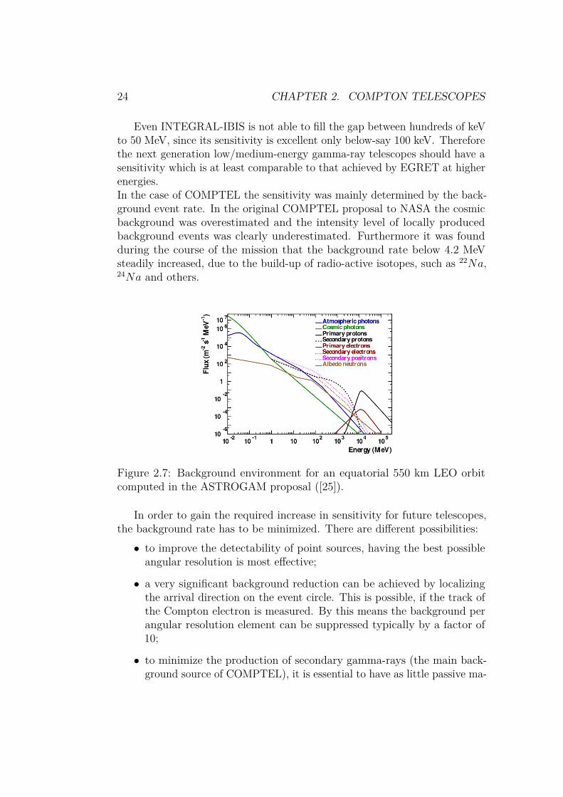
Figure 2.7: Background environment for an equatorial 550 km LEO orbitcomputed in the ASTROGAM proposal ([25]).
In order to gain the required increase in sensitivity for future telescopes,the background rate has to be minimized. There are different possibilities:• to improve the detectability of point sources, having the best possible
angular resolution is most effective;
• a very significant background reduction can be achieved by localizingthe arrival direction on the event circle. This is possible, if the track ofthe Compton electron is measured. By this means the background perangular resolution element can be suppressed typically by a factor of10;
• to minimize the production of secondary gamma-rays (the main back-ground source of COMPTEL), it is essential to have as little passive ma-
2.5. GENERAL GUIDELINES FOR A FUTURE COMPTON TELESCOPE25
terial around the instrument as possible, in order to reduce backgroundproduction inside the anticoincidence and guarantee best performance,optimizing angular and energy resolutions;
• optimization of ϕ-selection windows and windows for scatter angle direc-tions is another important and sensitive tool to reduce the background;
• the choice of the satellite orbit has a huge effect on the overall back-ground. In particular, in Low Earth Orbit (LEO) albedo will be thebiggest background source around 1 MeV (see Figure 2.7), while athigher orbits activation becomes a major issue.
2.5 General guidelines for a future ComptonTelescope
Several Compton space missions have been recently proposed (like the ESAmedium class mission ASTROGAM and the NASA medium class missionCOMPAIR, only to name the two leading proposals nowadays), and will bepresented again in an updated version in the coming years. However, all ofthese will rely on the silicon strip detector technology. Silicon trackers, largelyapplied to particle detection in the last two decades, provide good positionand energy resolution and abide by many items listed before for backgroundrejection.Therefore, the payload for a future telescope optimized for the MeV regime(as proposed by the ASTROGAM Collaboration, in 2015) will consists ofthree main detectors:
• A Silicon Tracker, in which the cosmic gamma rays undergo a firstCompton scattering or a pair conversion, based on the technology ofDouble Sided Si Strip Detectors (Si DSSDs) to measure the energy andthe position of each interaction with an excellent energy and spatialresolution;
• ACalorimetermade of scintillating crystals readout by photodetectors,to completely absorb all secondary particles and measure the interactionposition as well as the deposited energy. Thus it should be built ofhigh-Z material (e.g. CsI) and have good position and energy resolution;
• An Anticoincidence System design with plastic scintillators coveringthe whole instrument to detect single charged relativistic particleswith an efficiency exceeding 99.99% and to reject charged-particlesbackground events.

26 CHAPTER 2. COMPTON TELESCOPES
The payload is completed by the front-end electronics, the back-end elec-tronics, a payload data handling unit and a power supply unit. The Telescopewill operate in LEO, at a nominal height of 550 − 600 km, with a Field ofView ≥ 2.5 sr. It will achieve an angular resolution ≤ 1.5 and a sensitivity(for an observation time of 1 month) < 3 · 10−5 MeV cm−2 s−1 at 1 MeV.The COMPAIR collaboration is also examining the performances of a CZT-strip (Cadmium zinc telluride) calorimeter for the parts closest to the Tracker,where knowing the positions of the interacting low-energy Compton-scatteredphotons is very important. CZT calorimeters provide better spatial andenergy resolutions than CsI(Tl) calorimeters, but have much higher costs.
(a) ASTROGAM. (b) COMPAIR.
Figure 2.8: Schematic diagram for future Compton Telescopes, taken from[25] and [9].
Since the time scale for an M-class mission is around 10 years, with a cost∼ 500 Me, there is the actual opportunity for a small CubeSat Telescoperealization, with contained development costs, relatively quick design phase,to be used as a pathfinder test instrument for a future Compton Telescope.
Chapter 3
Silicon Tracker
3.1 Properties of a tracker for Compton Tele-scopes
As mentioned before, the tracker will be the heart of a future Telescopeoptimized in the MeV energy range, playing several tasks. First of all, it hasto act as a Compton scattering and pair creation medium. Therefore thematerial requires a large cross-section for these interactions and low Doppler-broadening; for both reasons a low Z material is preferred. Secondly, it hasto measure the direction of the secondary electrons and positrons as well astheir energy very accurately.
Semiconductor detectors provides good position and energy resolution, andrepresent the most logical choice for the Tracker of a future Compton Telescope.In particular Silicon Detectors are preferred to Germanium Detectors for thefollowing reasons:
• Silicon provides better angular resolution than Germanium assumingideal detector properties, as shown in Figure 3.1. On average, the angularresolution worsens with increasing Z, but it also strongly depends onthe shell structure of the individual atoms: the best FWHM is obtainedfor alkaline metals, while the worst FWHM is reached for noble gases,where orbitals are completely filled.
• Germanium detectors are very expensive and must be used at reducedtemperature for proper operation (usually the liquid nitrogen tempera-ture, 77.2 K). This fact is a great problem for space operations. LittleGe crystals detector is used in INTEGRAL-SPI however, for a spacetelescope, it is practically unrealizable to cover a great amount of volume
27

28 CHAPTER 3. SILICON TRACKER
with Germanium detectors. Moreover the cooler system contribute tothe increase of passive materials which activation could be a considerablesource of background.
• the Silicon strip detector technology was already applied to the detectionof gamma rays in space with the AGILE and Fermi-LAT missions.However, whereas AGILE and Fermi use Single Sided Strip Detectors(SSSDs), the tracker for a Compton Telescope needs Double Sided StripDetectors, in order to obtain precise information on electrons direction.
Figure 3.1: Angular resolution as a function of the atomic number Z, assumingideal detector properties ([30]).
Therefore a Compton telescope based on semiconductor technology shoulduse a Silicon tracker similar to the one used in Fermi-LAT, despite the energyresolution of Silicon is worse than that of Germanium.However there are some differences from the tracker for a Compton telescopewith respect to the one of Fermi-LAT. Firstly it should not have tungstenlayers (which act as converter material in FERMI-LAT tracker) and have anultra-light mechanical structure minimizing the amount of passive materialwithin the detection volume. This enables the tracking of low-energy Comp-ton electrons and reduce the effect of multiple Coulomb scattering and thebackground due to activation. Moreover a fine spatial resolution (< 1/6 ofthe microstrip pitch) is needed. These would be obtained by analog readoutof the signals, as for the AGILE tracker. Finally an ultra low-noise front-endelectronics is essential, in order to accurately measure the low energy depositsproduced by Compton events with an excellent spectral resolution.

3.2. NOISE IN A SILICON STRIP DETECTOR 29
In the design of a tracker for a future Compton telescope many parametersmust be carefully evaluated and tuned, like the number of the layers, thelayers thickness, the strip pitch etc.For example, a decrease of the strip pitch implies obviously a better spatialresolution. However it also implies the read-out of a much higher number ofchannel and then more power consumptions.Moreover a much higher sensitive volume achieved with the increasing of thenumber of layers, involves a considerable increase in the pay-load costs.The thickness of the silicon layers is an additional physical quantity that hasto be carefully evaluated. In fact, when a charged particle pass through thevolume of the silicon layer, undergoes several scattering due to the Coulombinteractions with lattice atoms. Usually to describe this phenomenon theaverage scattering angle is defined:
θ = 13.6MeVβcp
Z
√x
X0(3.1)
where X0 is the radiation length. Therefore, a much higher thickness forthe layers, is reflected to large particles deviation and a greater error thetrajectory reconstruction. Moreover the leakage current also increase. Instead,a much thick detector implies a smaller number of charge carriers and thedecrease of signals intensity.
3.2 Noise in a Silicon strip detectorThe key parameter for the design of a microstrip detector is the signal-to-noiseratio, S/N . In this section the various noise sources are described, and thedependence of the signal-to-noise ratio on the shaping time is discussed.
As illustrated in Figure 3.2, the detector is represented by the capacitanceCd and the detector bias voltage is applied through the bias resistor Rb. Forthe bias resistor holds the assumption Rb TP/Cd where TP is the peakingtime of the shaper. In other words the bias resistor must be sufficiently largein order to block the flow of signal charge. In this way all of the signal isavailable for the amplifier. The bypass capacitor Cb, serves to shunt anyexternal interference coming through the bias supply line to ground. Theseries resistor RS represents any resistance present in the connection from thedetector to the amplifier input, for example the resistance of the connectingwires, the resistance of the detector electrodes, etc. Finally the coupling

30 CHAPTER 3. SILICON TRACKER
capacitor Cc at the input of the amplifier can be neglected in our analysis,since the capacitor passes AC signals.
Figure 3.2: Detector front-end circuit (picture taken from [23]).
The electronic noise is usually expressed in term of the Equivalent NoiseCharge (ENC), i.e. the input charge for which S/N = 1. The electronics noisesources, differentiated in noise voltage sources and current noise sources, arehere summarized (a complete and thorough discussion of the argument canbe found in [23]):• Detector bias current. The noise current of the sensor is computedassuming that the input impedance of the amplifier is infinite, whilethe current that flow through Rb is negligible. The noise current willthen flow through the detector capacitance, yielding a voltage:
v2nd = 2qeId
1(ωCd)2 (3.2)
• Parallel resistance. The bias resistance Rb acts as a noise current source.In addition also the contribute of the sensor capacitance has to be takeninto account:
v2np = 4kTRb
1 + (ωRbCd)2 (3.3)
• Series resistance. The noise associated with the series resistance Rs issimply computed as:
v2nr = 4kTRs (3.4)
• Amplifier input noise voltage. The noise sources associated with anamplifier are a white noise component and a 1/f noise component.Then the equivalent noise voltage is:
v2na = v2
nw + Aff
(3.5)

3.2. NOISE IN A SILICON STRIP DETECTOR 31
In the case of a RC-CR shaper with equal differentiation and integrationtime constants (τi = τd ≡ τ), the equivalent noise charge can be computedvia the formula:
Q2n =
(ε2
8
)[(2eId + 4kT
Rb
+ i2na
)· τ + (4kTRS + e2
na) ·C2d
τ+ 4AfC2
d
](3.6)
In order to reach a good estimation of the equivalent noise ratio for thetracker designed in this thesis, the physical quantities in 3.6 was evaluatedfor a suitable microtrip detector (e.g. the silicon microstrip detector used inFERMI-LAT mission) and read-out electronics (e.g. the ASIC VATA460,[10]).The physical quantities settled for the equivalent noise ratio computation arelisted in Table 3.1.
Parameter ValueT 300 KId 10 nARb 40 MΩina 0.2 pA/
√Hz
ena 5 nA/√
HzAf 10−11 V2
Rs 400 ΩCd 10 pF
Table 3.1: Parameters used for the equivalent noise charge estimation.
Peaking time (s)8−10 7−10 6−10 5−10
EN
C (
e)
210
310
410
ENC as a function of CR-RC peaking time.I_dR_pnaiR_s
nae1/fTotal
Figure 3.3: Equivalent noise charge as a function of the CR-RC peaking time.
The dependence of the ENC on the CR-RC peaking time is shown inFigure 3.3. As we can see voltage sources are the most important noise

32 CHAPTER 3. SILICON TRACKER
source for short peaking times, while at long peaking times the current noisesources dominate. A minimum is reached when the current and voltage noisecontributions are equal.Since the shaping time of VATA460 is ∼ 2µs, we can correctly assume anequivalence noise charge of 1100− 1200 e− for our future tracker design.

Chapter 4
Detector design andsimulations
4.1 The MEGAlib software packageSimulations are an essential analysis tool in physics, and play a fundamentalrole in the development and design of X and gamma-ray telescopes, inparticular. In fact they allow determining the performance of the detectorswith respect to the desired science objectives. In addition, they enable theoptimization of the design by performing trade-off studies between variationsof the detector setup, various instrument orbits, optimization of passivematerials, and many more. Finally, simulations help to prepare and tounderstand calibrations and measurements of the instrument.In this work simulations are made using the simulation and data analysis toolMEGAlib (the Medium Energy Gamma-ray Astronomy library), developedby Andreas Zoglauer. The MEGAlib software package is completely writtenin C++ and utilizes the ROOT software library for its graphical user interfaceand its data display. Its main application area is hard X-ray and low-to-medium-energy gamma-ray telescopes, from a few keV up to hundreds of MeV.MEGAlib encompasses the complete data analysis pipeline from simulationsto high-level data analysis, thanks to its four principal libraries:
1. Geomega (Geometry for MEGAlib). Geomega is the universalgeometry and detector description library of MEGAlib, for the detailedmodeling of different detector types: 2D or 3D strip detectors, driftchambers, calorimeters. The geometry file has to include the descriptionof all materials, volumes and detectors properties of the telescopes(energy resolutions, noise properties, trigger criteria, etc.);
2. Cosima (Cosmic Simulator for MEGAlib). Cosima is the simula-
33
34 CHAPTER 4. DETECTOR DESIGN AND SIMULATIONS
tion tool of MEGAlib. It is based on Geant4 and provides the generationof simulated data, via electromagnetic (Livermore and Penelope) orhadronic libraries. In this work the Livermore library is used for the sim-ulation of monochromatic point-like photon sources at different energies,and diffuse sources;
3. Revan (Real Event Analyzer). Revan provides the events recon-struction using the detector characteristics and the energy and positioninformations of individual hits. Its task is to identify the original inter-action process such as photo effect, Compton scattering, pair creation,radioactive decay etc. This is a crucial step in the data-analysis frame-work since the overall performance of a Compton telescope is not onlydetermined by its hardware but also by the performance of the algo-rithms which recover the original parameters of the incident photonsfrom the measured (or simulated) data. In fact each not recognized orincorrectly reconstructed event lowers the efficiency and increases thebackground of the instrument, affecting the final sensitivity estimationof the telescope. Revan events reconstruction tries to identify the mostsimple structures like pair events and muons first; searching for themuch more complex structures of Compton events in the remainingevents. The events reconstruction process consists of four main steps:
• Clusterize into one hit the single passing particle interactions intwo or more adjacent voxels of a strip or pixel detector;
• Search for high energy events like a vertex of the pair events or amuon tracks;
• Search for Compton electron tracks and the Compton interactionsequences;
• Search for special beta-decays.
4. Mimrec (MEGAlib image reconstruction) Mimrec is MEGAlib’smain tool for advanced data analysis. It enables event selections onvarious parameters of Compton and pair events, and provides anal-ysis of energy spectra, ARM distributions, Compton and pair imagereconstruction etc.
Moreover, during the thesis work, several scripts and macros were written inC++ and Python, in order to reach much more control on various parametersand kinematic variables.

4.2. DEFINING DETECTOR’S GEOMETRY: STARTING GEOMETRY35
4.2 Defining detector’s geometry: Startinggeometry
As mentioned before, the purpose of the thesis is to design and evaluate theperformances of a CubeSat Compton Telescope. A CubeSat is a standardizedmodel of miniaturized satellite for space research, with precise restrictionsboth in volume and in weight: it consist in a 10 × 10 × 10 cm3 cube witha maximum weight of 1.33 kg (1U cubesat). It is possible to increase thecubesat length of one axis, adding one unit of the same dimensions. Thus a2U cubesat (10×10×20 cm3) or a 3U cubesat (10×10×30 cm3) can be realized.
The telescope fundamental design, shown in Figure 4.1, is composed oftwo main detectors: a silicon strip tracker unit, with the dimensions of8.4 × 8.4 × 7.5 cm3 on the upper half, and a CsI(Tl) calorimeter, with thedimensions of 8.9 × 8.9 × 5 cm3 on the lower half, leaving some space forstructural elements, electronics and other passive materials (not consideredat this stage). The first design was settled "back of the envelope", makingseveral educated guesses which evaluated both performance and costs.
Figure 4.1: Schematic diagram of the telescope starting geometry.
The tracker, which fundamental parameters are listed in Table 4.1, is
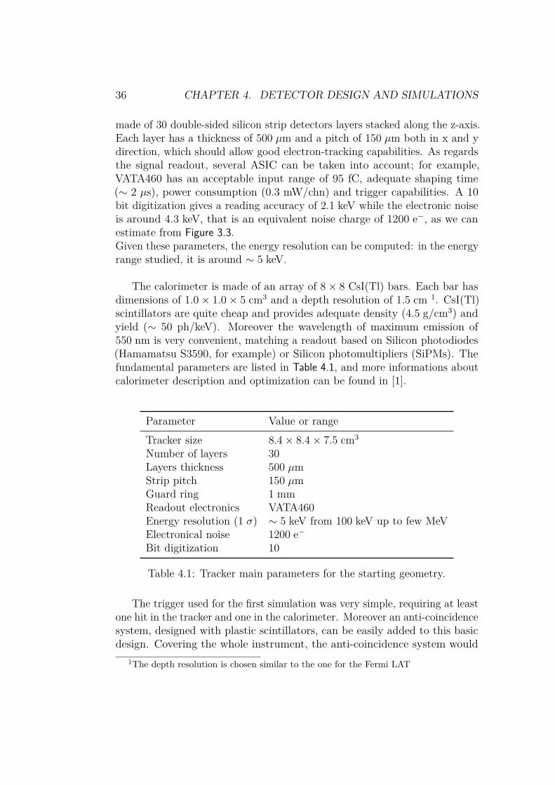
36 CHAPTER 4. DETECTOR DESIGN AND SIMULATIONS
made of 30 double-sided silicon strip detectors layers stacked along the z-axis.Each layer has a thickness of 500 µm and a pitch of 150 µm both in x and ydirection, which should allow good electron-tracking capabilities. As regardsthe signal readout, several ASIC can be taken into account; for example,VATA460 has an acceptable input range of 95 fC, adequate shaping time(∼ 2 µs), power consumption (0.3 mW/chn) and trigger capabilities. A 10bit digitization gives a reading accuracy of 2.1 keV while the electronic noiseis around 4.3 keV, that is an equivalent noise charge of 1200 e−, as we canestimate from Figure 3.3.Given these parameters, the energy resolution can be computed: in the energyrange studied, it is around ∼ 5 keV.
The calorimeter is made of an array of 8× 8 CsI(Tl) bars. Each bar hasdimensions of 1.0× 1.0× 5 cm3 and a depth resolution of 1.5 cm 1. CsI(Tl)scintillators are quite cheap and provides adequate density (4.5 g/cm3) andyield (∼ 50 ph/keV). Moreover the wavelength of maximum emission of550 nm is very convenient, matching a readout based on Silicon photodiodes(Hamamatsu S3590, for example) or Silicon photomultipliers (SiPMs). Thefundamental parameters are listed in Table 4.1, and more informations aboutcalorimeter description and optimization can be found in [1].
Parameter Value or rangeTracker size 8.4× 8.4× 7.5 cm3
Number of layers 30Layers thickness 500 µmStrip pitch 150 µmGuard ring 1 mmReadout electronics VATA460Energy resolution (1 σ) ∼ 5 keV from 100 keV up to few MeVElectronical noise 1200 e−
Bit digitization 10
Table 4.1: Tracker main parameters for the starting geometry.
The trigger used for the first simulation was very simple, requiring at leastone hit in the tracker and one in the calorimeter. Moreover an anti-coincidencesystem, designed with plastic scintillators, can be easily added to this basicdesign. Covering the whole instrument, the anti-coincidence system would
1The depth resolution is chosen similar to the one for the Fermi LAT

4.3. FIRST SIMULATIONS 37
detect single charged particles with an efficiency of 99.99%, and veto nearlyall the charged particle background. At this stage no ACD was considered inthis design.
Parameter Value or rangeCalorimeter size 8.9× 8.9× 5 cm3
CsI(Tl) bars dimension 1.0× 1.0× 5 cm3
Photodiode readout Hamamatsu S3590Readout electronics VATA460Depth resolution 1.5 cmEnergy resolution (1 σ) from 10 keV at 100 keV to 25 keV at 2 MeV
Table 4.2: Calorimeter main parameters for the starting geometry.
4.3 First simulationsThe geometry defined in the previous section was tested using Cosima, simu-lating the detectors response under a monochromatic point-like photon sourceat normal incidence and at different energies: 100, 333, 500, 1000, 2000 keV.In this way the behavior and the performance of the telescope as a functionof the energy, can be analyzed. For each set of simulations we are interested,in particular, in the energy and ARM (Angular Resolution Measure) spectraof the reconstructed photon. In fact, from these spectra, some of the funda-mental parameters for the characterization of the detector as the energy andangular resolution, and the effective area can be obtained.
htempEntries 216723Mean 104RMS 11.94
Energy (keV)60 80 100 120 140
Cou
nts
0
500
1000
1500
2000
2500
3000
3500
4000
htempEntries 216723Mean 104RMS 11.94
Energy spectrum
(a) Energy spectrum.
htempEntries 216723Mean 30.48− RMS 41.84
ARM (deg)200− 150− 100− 50− 0 50 100 150
Cou
nts
0
500
1000
1500
2000
2500
3000
3500
htempEntries 216723Mean 30.48− RMS 41.84
ARM spectrum
(b) ARM spectrum.
Figure 4.2: Energy and ARM spectra for the 100 keV simulation with thestarting geometry.
38 CHAPTER 4. DETECTOR DESIGN AND SIMULATIONS
htempEntries 631495Mean 317.2RMS 48.1
Energy (keV)50 100 150 200 250 300 350 400 450
Cou
nts
0
5000
10000
15000
20000
25000htemp
Entries 631495Mean 317.2RMS 48.1
Energy spectrum
(a) Energy spectrum.
htempEntries 631495Mean 0.886− RMS 21.84
ARM (deg)150− 100− 50− 0 50 100 150
Cou
nts
0
5000
10000
15000
20000
25000
30000
35000
40000
45000
htempEntries 631495Mean 0.886− RMS 21.84
ARM spectrum
(b) ARM spectrum.
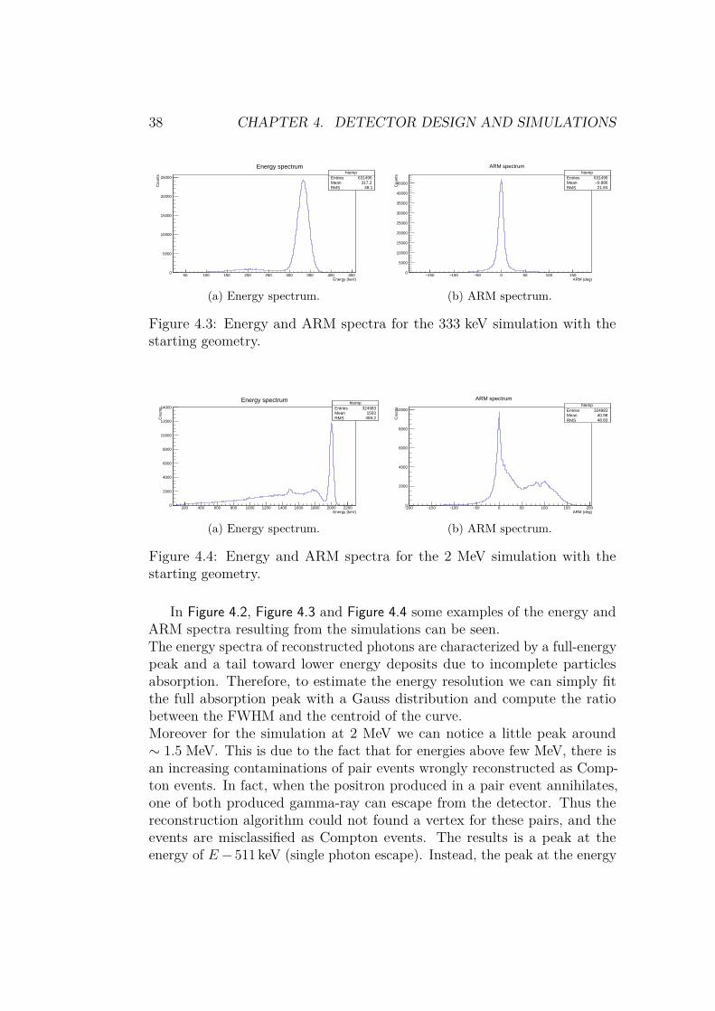
Figure 4.3: Energy and ARM spectra for the 333 keV simulation with thestarting geometry.
htempEntries 324983Mean 1503RMS 469.2
Energy (keV)200 400 600 800 1000 1200 1400 1600 1800 2000 2200
Cou
nts
0
2000
4000
6000
8000
10000
12000
14000htemp
Entries 324983Mean 1503RMS 469.2
Energy spectrum
(a) Energy spectrum.
htempEntries 324983Mean 40.98RMS 48.83
ARM (deg)200− 150− 100− 50− 0 50 100 150 200
Cou
nts
0
2000
4000
6000
8000
10000htemp
Entries 324983Mean 40.98RMS 48.83
ARM spectrum
(b) ARM spectrum.
Figure 4.4: Energy and ARM spectra for the 2 MeV simulation with thestarting geometry.
In Figure 4.2, Figure 4.3 and Figure 4.4 some examples of the energy andARM spectra resulting from the simulations can be seen.The energy spectra of reconstructed photons are characterized by a full-energypeak and a tail toward lower energy deposits due to incomplete particlesabsorption. Therefore, to estimate the energy resolution we can simply fitthe full absorption peak with a Gauss distribution and compute the ratiobetween the FWHM and the centroid of the curve.Moreover for the simulation at 2 MeV we can notice a little peak around∼ 1.5 MeV. This is due to the fact that for energies above few MeV, there isan increasing contaminations of pair events wrongly reconstructed as Comp-ton events. In fact, when the positron produced in a pair event annihilates,one of both produced gamma-ray can escape from the detector. Thus thereconstruction algorithm could not found a vertex for these pairs, and theevents are misclassified as Compton events. The results is a peak at theenergy of E− 511 keV (single photon escape). Instead, the peak at the energy
4.3. FIRST SIMULATIONS 39
of E − 1022 keV (double photon escape) is not observed in our simulations,since the escape of both photon is a quite unlikely circumstance, especiallyin the energy range studied. Obviously these wrongly reconstructed eventscontribute also to the tails in the ARM distribution.
The ARM spectra are a bit more complex, since they can exhibit leftor right tails, due to incompletely absorbed scattered gamma ray and recoilelectron, respectively. These phenomena are remarkable especially at lowerenergies (∼ 100 keV) and at higher energies (∼ 2000 keV). As a consequence,the shape of the peak is affected by the tails of poorly reconstructed eventsand can not be correctly fitted by any simple distribution, neither a Gauss ora Lorentz distribution. A quite good estimation of the peak FWHM can beobtained with a fit of two different gauss distributions to take into accountthe different tails for each side of the peak.
Finally, the effective area Aeff can be computed using the formula:
Aeff = AstartNmeasured
Nsimulated
(4.1)
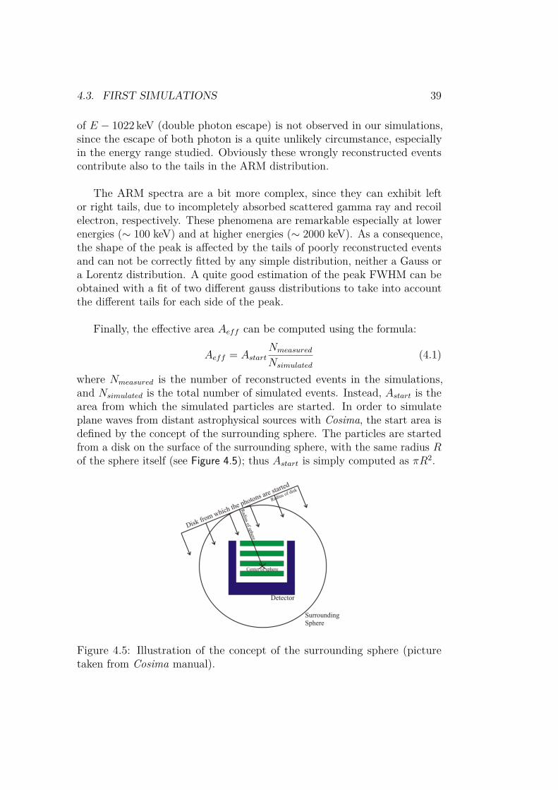
where Nmeasured is the number of reconstructed events in the simulations,and Nsimulated is the total number of simulated events. Instead, Astart is thearea from which the simulated particles are started. In order to simulateplane waves from distant astrophysical sources with Cosima, the start area isdefined by the concept of the surrounding sphere. The particles are startedfrom a disk on the surface of the surrounding sphere, with the same radius Rof the sphere itself (see Figure 4.5); thus Astart is simply computed as πR2.
Figure 4.5: Illustration of the concept of the surrounding sphere (picturetaken from Cosima manual).

40 CHAPTER 4. DETECTOR DESIGN AND SIMULATIONS
In Table 4.3 the telescope main parameters are shown as a function ofsimulated energy.In this phase of the work the errors are only statistical and not particu-larly significant (they can be reduced at discretion increasing the numberof simulated events). Under these conditions systematic errors are morerelevant, but in this preliminary stage of the work they were not studied(the final structure of the detector is not decided yet, no passive materialswere included in the design etc.). In the completely settled design wherethe detectors characteristics, the read-outs and the electronics performancesare all decided and evaluated, it will be possible to carefully compute thesystematic errors.
Energy [keV] Aeff [cm2] Energy resolution (FWHM) ARM FWHM []100 1.43 24% 51.5333 3.90 9.3% 12.9500 3.62 6.8% 9.91000 2.81 4.2% 8.62000 2.49 2.7% 11.5
Table 4.3: Telescope performances for the starting geometry.
The obtained performances are very sensitive to energy. The effectivearea increases rapidly from 100 keV to 333 keV and then starts to slowlydecrease, due to the lowering of Compton cross section at higher energies. Atthe same time, the energy resolutions and the ARM FWHM greatly improvefrom 100 keV to 333 keV. Even considering these preliminary results, we cansee that the 100 keV energy establish the lower limit for the CubeSat design.Instead, the higher limit is set to energies of few MeV, since already at 2 MeVthe rate of wrongly reconstructed events starts to increase (as it can be seenfrom the tails in the energy and ARM spectra in Figure 4.4).
4.4 Only-calorimeter geometryBefore moving on with the analysis and the optimization of the detector, itis interesting to understand, in a very simple but straightforward way, howmuch the presence of the silicon tracker affect the overall performance of thetelescope.

4.4. ONLY-CALORIMETER GEOMETRY 41
Energy (keV)210 310
)2E
ffect
ive
area
(cm
0
10
20
30
40
50
Effective areas comparison plot
only-calorimeter geometry
starting geometry
Figure 4.6: Comparison of the effective areas estimated from only-calorimeterconfiguration and starting configuration.
To achieve this scope an only-calorimeter geometry, made only of an18× 18 array of 0.5× 0.5× 10 cm3 CsI(Tl) crystals was tested. Obviouslythis is a quite unrealistic design; nevertheless such a simple geometry can giveimportant informations about the necessity of the presence of the tracker.As we can easily expect, the effective area of the only-calorimeter geometry ismuch bigger than the one computed for the starting geometry (Figure 4.6).However the increase of the effective area is followed by a remarkable wors-ening of the ARM spectra for different energies. As we can see in Figure 4.7and Figure 4.8, many wrongly reconstructed events contribute not only tothe increase of the tails of the distributions, but also to the broadening ofthe peak. In fact, in order to give just a rough estimation, if in the startinggeometry the ARM FWHM is around ∼ 10 for energies above 100 keV, inthe only-calorimeter geometry the FWHM is around 25 − 30.
htempEntries 288520Mean 16.39RMS 55.09
ARM (deg)-150 -100 -50 0 50 100 150
Cou
nts
0
500
1000
1500
2000
2500
3000
3500
htempEntries 288520Mean 16.39RMS 55.09
ARM spectrumhtemp
Entries 631495Mean 0.886− RMS 21.84
ARM (deg)150− 100− 50− 0 50 100 150
Cou
nts
0
5000
10000
15000
20000
25000
30000
35000
40000
45000
htempEntries 631495Mean 0.886− RMS 21.84
ARM spectrum
Figure 4.7: Comparison of the ARM spectrum from only calorimeter configu-ration (left) and starting configuration (right), for a 333 keV simulation.

42 CHAPTER 4. DETECTOR DESIGN AND SIMULATIONS
htempEntries 325604Mean 42.06RMS 57.66
ARM (deg)200− 150− 100− 50− 0 50 100 150 200
coun
ts
0
500
1000
1500
2000
2500
3000
htempEntries 325604Mean 42.06RMS 57.66
ARMhtemp
Entries 406896Mean 23.42RMS 45.02
ARM (deg)200− 150− 100− 50− 0 50 100 150 200
Cou
nts
0
2000
4000
6000
8000
10000
12000
htempEntries 406896Mean 23.42RMS 45.02
ARM
Figure 4.8: Comparison of the ARM spectrum from only calorimeter configu-ration (left) and starting configuration (right), for a 1 MeV simulation.
Finally, there are not great differences in the energy spectra of the twoconfigurations (in Figure 4.9 an example for the simulation at 1 MeV ispresented). Therefore from these simulations we have a straightforwardindication of the importance of a silicon tracker.
htempEntries 325604Mean 785.6RMS 258.4
Energy (keV)0 200 400 600 800 1000 1200
coun
ts
0
2000
4000
6000
8000
10000htemp
Entries 325604Mean 785.6RMS 258.4
Energy
htempEntries 406896Mean 843.7RMS 226.1
Energy (kev)0 200 400 600 800 1000
coun
ts
0
2000
4000
6000
8000
10000
12000
14000
16000 htempEntries 406896Mean 843.7RMS 226.1
Energy
Figure 4.9: Comparison of the energy spectrum from only calorimeter config-uration (left) and starting configuration (right), for a 1 MeV simulation.
4.5 Lateral calorimeter geometry
In the starting geometry a significant fraction of events are lost at the edge ofthe tracker, as it can be seen in Figure 4.10, where the events projection on thex-y plane for a 333 keV simulation is shown. This is due to the fact that forenergies below 1 MeV the majority of photons are scattered to angles > |30|(see the Klein-Nishina cross section in Figure 1.5). Thus, there is a high proba-bility that the scattered particles escape the detector without leaving any hits.

4.5. LATERAL CALORIMETER GEOMETRY 43
x position (cm)-4 -3 -2 -1 0 1 2 3 4
y po
sitio
n (c
m)
-4
-3
-2
-1
0
1
2
3
4
0
20
40
60
80
100
120
140
160
180
200
Tracker events
Figure 4.10: Events distribution in the x-y plane for a 333 keV simulation.
Therefore we decided to study in more detail a new geometry, including alateral calorimeter made of 1.0× 1.0× 8.1 cm3 CsI crystal, decreasing the x-ysize of the tracker and the bottom calorimeter (see Figure 4.11)2.In particular we tested two configurations: in the first one (we will name itlateral calorimeter 1 geometry) the starting detector size was decreased of0.8 cm both in x and y direction; in the second one (named lateral calorimeter2 geometry) the x and y size was reduced of 1.8 cm.
Figure 4.11: Schematic diagram of the telescope final geometry.
2we decreased the tracker and bottom calorimeter sizes in order to still have a configu-ration compatible to a 2 mathrmU CubeSat

44 CHAPTER 4. DETECTOR DESIGN AND SIMULATIONS
As shown in Figure 4.12, the effective area estimated for both configurationsincreases compared to the one estimated for the starting geometry. Howeverthe effective area of the lateral calorimeter 1 configuration is greater thanthe one estimated for the lateral calorimeter 2 configuration. The energy andARM FWHM, instead, are comparable for each configuration.The considerable increase in the effective area achieved with the introductionof lateral CsI(Tl) crystals, brings the choice of the detector geometry to asatisfying stage. In fact, from our analysis the best configuration is lateralcalorimeter 1 geometry, since a design with a more effective area is, of course,preferable under comparable values for the others final parameters of spacetelescope, as the energy and angular resolution.
log E (keV)210 310
)2
effe
ctiv
e ar
ea (
cm
0
1
2
3
4
5
6
7
8
9
10no lat cal
lat cal 1
lat cal 2
Figure 4.12: Effective area estimated from simulations with and withoutlateral calorimeters.
Energy [keV] Aeff [cm2] Energy resolution (FWHM) ARM FWHM []100 7.09 25% 55.4333 8.67 9.3% 14.6500 6.87 6.9% 11.11000 5.81 4.4% 10.92000 4.95 2.8% 13.7
Table 4.4: Telescope performances for the lateral calorimeter geometry.
In Table 4.4 the telescope main parameters for this final geometry areshown as a function of simulated energy. In comparison to COMPTEL, in theenergy range around 1 MeV, the detector developed in this thesis can provide
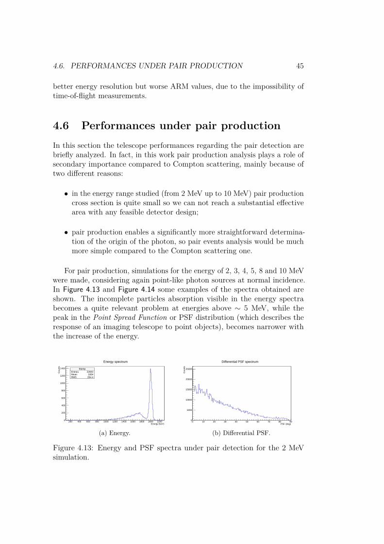
4.6. PERFORMANCES UNDER PAIR PRODUCTION 45
better energy resolution but worse ARM values, due to the impossibility oftime-of-flight measurements.
4.6 Performances under pair productionIn this section the telescope performances regarding the pair detection arebriefly analyzed. In fact, in this work pair production analysis plays a role ofsecondary importance compared to Compton scattering, mainly because oftwo different reasons:
• in the energy range studied (from 2 MeV up to 10 MeV) pair productioncross section is quite small so we can not reach a substantial effectivearea with any feasible detector design;
• pair production enables a significantly more straightforward determina-tion of the origin of the photon, so pair events analysis would be muchmore simple compared to the Compton scattering one.
For pair production, simulations for the energy of 2, 3, 4, 5, 8 and 10 MeVwere made, considering again point-like photon sources at normal incidence.In Figure 4.13 and Figure 4.14 some examples of the spectra obtained areshown. The incomplete particles absorption visible in the energy spectrabecomes a quite relevant problem at energies above ∼ 5 MeV, while thepeak in the Point Spread Function or PSF distribution (which describes theresponse of an imaging telescope to point objects), becomes narrower withthe increase of the energy.
htempEntries 22663Mean 1804RMS 264.4
Energy (keV)200 400 600 800 1000 1200 1400 1600 1800 2000 2200
Cou
nts
0
200
400
600
800
1000
1200
1400 htempEntries 22663Mean 1804RMS 264.4
Energy spectrum
(a) Energy.PSF (deg)
0 10 20 30 40 50 60 70 80 90
Cou
nts
0
5000
10000
15000
20000
25000
Differential PSF spectrum
(b) Differential PSF.
Figure 4.13: Energy and PSF spectra under pair detection for the 2 MeVsimulation.

46 CHAPTER 4. DETECTOR DESIGN AND SIMULATIONS
htempEntries 60482Mean 4011RMS 726.7
Energy (keV)0 1000 2000 3000 4000 5000
Cou
nts
0
200
400
600
800
1000
1200
1400
htempEntries 60482Mean 4011RMS 726.7
Energy spectrum
(a) Energy.PSF (deg)
0 10 20 30 40 50 60 70 80 90
Cou
nts
0
20
40
60
80
100
120
140
160
180
310×Differentail PSF spectrum
(b) Differential PSF.
Figure 4.14: Energy and PSF spectra under pair detection for the 5 MeVsimulation.
The effective area obtained from the pair simulations is compared to theone associated to Compton scattering events in Figure 4.15: the effectivearea for pair events is actually quite small. Moreover, for the energies above5 MeV, a significant fraction of incompletely absorbed events affects the valuesobtained, and the peaks due to the escape of one or both photons in positronannihilation events are very pronounced.
Energy (keV)210 310 410
)2E
ffect
ive
area
(cm
0
1
2
3
4
5
6
7
8
9
Effective area plot
compton
pair production
Figure 4.15: Comparison of the effective area for Compton scattering andpair production.
On the other hand the PSF can be easily improved applying quite simplecuts: cuts in the direction of positrons and electrons were performed, excludingevents with a small angle with the tracker plane. The PSF containmentintervals greatly improved (from the red to the green line, and from the blackto the blue line in Figure 4.16) discarding no more than 20 − 25% of thetotal events. Another task of quality cuts is to remove misclassified Comptonevents, which is important especially at lower energies.

4.6. PERFORMANCES UNDER PAIR PRODUCTION 47
Energy (keV)2000 3000 4000 5000 6000 7000 8000 9000 10000
PS
F in
terv
als
(deg
)
0
10
20
30
40
50
60
70
80
90
68% interval
68% interval cut
95% interval
95% interval cut
PSF intervals comparison plot
Figure 4.16: PSF containment intervals before and after quality cuts.

48 CHAPTER 4. DETECTOR DESIGN AND SIMULATIONS

Chapter 5
Event selection and trackeroptimization in the Comptonregime
5.1 Tracked events and event selectionIn Chapter 4 the telescope geometry was defined and the general perfor-mances were estimated with satisfying results. In this chapter we want toperform further analyses. We only considered Compton scattered events,ignoring performance of reconstructions of pairs (as explained before pairproduction plays a role of secondary importance compared to Compton scat-tering in our detector design). We selected and divided the total events inevent classes. In particular tracked events present a very different topologyrespect to not tracked events.
htempEntries 196960Mean 825.2RMS 254.4
Energy (keV)0 200 400 600 800 1000 1200
Cou
nts
0
2000
4000
6000
8000
10000htemp
Entries 196960Mean 825.2RMS 254.4
Energy spectrum
(a) Energy.
htempEntries 196960Mean 27.71RMS 50.41
ARM (deg)-200 -150 -100 -50 0 50 100 150 200
Cou
nts
0
1000
2000
3000
4000
5000
htempEntries 196960Mean 27.71RMS 50.41
ARM spectrum
(b) Differential ARM.
Figure 5.1: Energy and ARM spectra for tracked and not tracked events in a1 MeV simulation.
49

50CHAPTER 5. EVENT SELECTION AND TRACKER OPTIMIZATION
In Figure 5.1 tracked and not tracked events are plotted for the 1 MeVsimulation: in blue are represented total events, in black not tracked eventsand in red tracked events. As we can see, tracked events represent only asmall fraction of the total data. Moreover the ARM distribution does notexhibit the left and right tails due to incompletely absorbed events, but itpresent a broadened peak.In addition to the energy resolution and the ARM FWHM, another parametercan be computed for tracked events: the Scatter Plane Deviation or SPD.In Figure 5.2 an example of SPD distribution for a 1 MeV simulation is plotted.As is can be seen, for tracked events the SPD HWHM is around roughly30− 40, depending on energy. Otherwise, for not tracked events, the SPDHWHM is set to 180. Therefore tracked events can still provide much betterinformations compared to not tracked events, despite the broadening of ARMpeak.
htempEntries 40898Mean 51.91RMS 52.02
SPD (deg)0 20 40 60 80 100 120 140 160 180
Cou
nts
0
100
200
300
400
500
600
700
800
900
htempEntries 40898Mean 51.91RMS 52.02
SPD spectrum
Figure 5.2: SPD distribution for a 1 MeV simulation.
Thus, to further improve our analysis, we decided to divide the eventsreconstructed in simulations in four different event classes:
• class 1 events: events with a track and at least one hit in the bottomcalorimeter, but no hits in the lateral calorimeter. The parametersestimated for this events class are plotted in blue in the followingfigures of this chapter;
• class 2 events: events with a track and at least one hit in the lateralcalorimeter, but no hits in the bottom calorimeter. The parametersestimated for this events class are plotted in black in the followingfigures;

5.1. TRACKED EVENTS AND EVENT SELECTION 51
• class 3 events: events with a single hit in the silicon tracker (thus nottracked) and at least one hit in the bottom calorimeter, but no hitsin the lateral one. The parameters estimated for this events class areplotted in red in the following figures;
• class 4 events: events with a single hit in the silicon tracker (nottracked) and at least one hit in the lateral calorimeter, but no hits inthe bottom one. The parameters estimated for this events class areplotted in green in the following figures.
We omitted in our analysis tracked and not tracked events with hits bothin the bottom and in the lateral calorimeter, since they hardly representproperly reconstructed events in our configuration, that constitute only asmall fraction of total events. We also omitted events with hits in the lateraland in the bottom calorimeter but with no hits in the tracker, since theperformances are worse and in this work we are interested in optimizing thesilicon tracker performance.
Energy (keV)200 400 600 800 1000 1200 1400 1600 1800 2000
)2E
ffect
ive
Are
a (c
m
0
1
2
3
4
5
6
Effective Area for different events classes
Tracked + Bottom Calorimeter
Tracked + Lateral Calorimeter
Hit Tracker + Bottom Calorimeter
Hit Tracker + Lateral Calorimeter
(a) Effective area.Energy (keV)
200 400 600 800 1000 1200 1400 1600 1800 2000
Ene
rgy
reso
lutio
n (%
)
5
10
15
20
25
Energy resolution for different events classes
Tracked + Bottom Calorimeter
Tracked + Lateral Calorimeter
Hit Tracker + Botton Calorimeter
Hit Tracker + Lateral Calorimeter
(b) Energy resolution.
Energy (keV)200 400 600 800 1000 1200 1400 1600 1800 2000
AR
M F
WH
M (
deg)
20
30
40
50
60
70
ARM for different events classes
Tracked + Bottom Calorimeter
Tracked + Lateral Calorimeter
Hit Tracker + Bottom Calorimeter
Hit Tracker + Lateral Calorimeter
(c) ARM FWHM.Energy (keV)
400 600 800 1000 1200 1400 1600 1800 2000
SP
D H
WH
M (
deg)
22
24
26
28
30
32
34
36
38
40
SPD for different events classes
Tracked + Bottom Calorimeter
Tracked + Lateral Calorimeter
(d) SPD HWHM.
Figure 5.3: Parameters estimated for the standard configuration.
In Figure 5.3 the main telescope parameters are plotted as a function ofenergy for each different class considered. The fit of the ARM and energy

52CHAPTER 5. EVENT SELECTION AND TRACKER OPTIMIZATION
spectra were made as explained in Chapter 4, while the fit of the SPDdistribution was performed via an half-gaussian. As we can see, the energyresolutions are nearly the same for all event classes, while tracked eventspresent an ARM FWHM highly worse than not tracked events. In fact inorder to generate an electron track, a sufficient amount of energy needs tobe transferred to the electron. This results in large Compton scatter angles,where energy measurements uncertainties have a larger influence on the angu-lar resolution than at small Compton scatter angles.
Moreover some points are not present in the figures. In fact in the case ofthe 100 keV energy, we do not have any tracked events, since an electron withenergy smaller than a hundred of keV is completely absorbed in a 500 µm thicksilicon layer. Instead, at higher energies the 1 cm thick lateral calorimetercan not completely absorb the scattered particles, so a fit of the ARM spectracould be very difficult due to the large presence of the tails in the distribution.
Parameter Simulated valuesLayers number 20, 25, 30Layers thickness 400, 500, 600 µmLayers pitch 50, 150, 300 µmBit digitization 8, 10, 12Equivalent noise charge 600, 1200, 2400 e−
Table 5.1: Parameters considered for the silicon tracker optimization. In boldare reported the parameters used in the standard configuration.
In order to optimize the tracker design, and validate the characteristicsand the specifics settled in Chapter 4, related both to the detector designand the read-out electronics, many simulations were performed. Startingfrom the standard configuration defined in the previous chapter, we stressedtime by time a single physical quantity (as the number of tracker layers, thepitch of the strip, the noise level etc.) and computed the main parametersuseful to define the telescope performance. In Table 5.1 are listed the physicalquantities considered in the simulations and the values investigated.
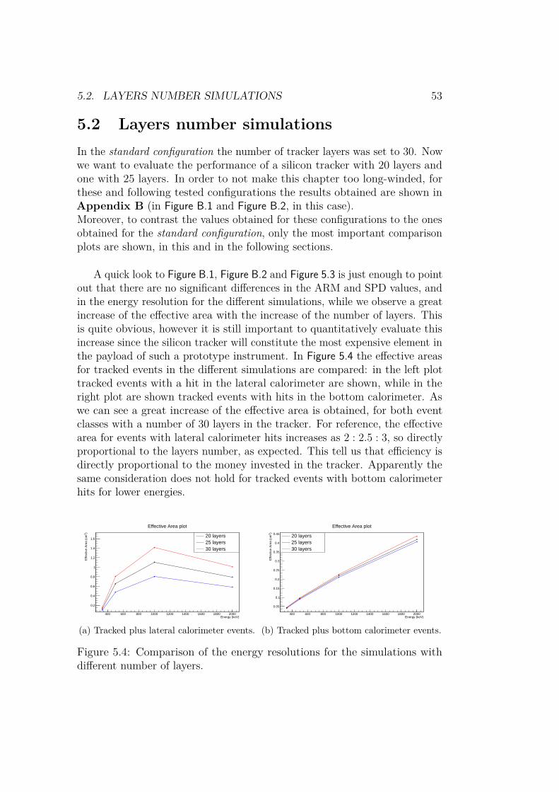
5.2. LAYERS NUMBER SIMULATIONS 53
5.2 Layers number simulationsIn the standard configuration the number of tracker layers was set to 30. Nowwe want to evaluate the performance of a silicon tracker with 20 layers andone with 25 layers. In order to not make this chapter too long-winded, forthese and following tested configurations the results obtained are shown inAppendix B (in Figure B.1 and Figure B.2, in this case).Moreover, to contrast the values obtained for these configurations to the onesobtained for the standard configuration, only the most important comparisonplots are shown, in this and in the following sections.
A quick look to Figure B.1, Figure B.2 and Figure 5.3 is just enough to pointout that there are no significant differences in the ARM and SPD values, andin the energy resolution for the different simulations, while we observe a greatincrease of the effective area with the increase of the number of layers. Thisis quite obvious, however it is still important to quantitatively evaluate thisincrease since the silicon tracker will constitute the most expensive element inthe payload of such a prototype instrument. In Figure 5.4 the effective areasfor tracked events in the different simulations are compared: in the left plottracked events with a hit in the lateral calorimeter are shown, while in theright plot are shown tracked events with hits in the bottom calorimeter. Aswe can see a great increase of the effective area is obtained, for both eventclasses with a number of 30 layers in the tracker. For reference, the effectivearea for events with lateral calorimeter hits increases as 2 : 2.5 : 3, so directlyproportional to the layers number, as expected. This tell us that efficiency isdirectly proportional to the money invested in the tracker. Apparently thesame consideration does not hold for tracked events with bottom calorimeterhits for lower energies.
Energy (keV)400 600 800 1000 1200 1400 1600 1800 2000
)2E
ffect
ive
Are
a (c
m
0.2
0.4
0.6
0.8
1
1.2
1.4
1.6
Effective Area plot
20 layers25 layers30 layers
(a) Tracked plus lateral calorimeter events.Energy (keV)
400 600 800 1000 1200 1400 1600 1800 2000
)2E
ffect
ive
Are
a (c
m
0.05
0.1
0.15
0.2
0.25
0.3
0.35
0.4
0.45
Effective Area plot
20 layers25 layers30 layers
(b) Tracked plus bottom calorimeter events.
Figure 5.4: Comparison of the energy resolutions for the simulations withdifferent number of layers.

54CHAPTER 5. EVENT SELECTION AND TRACKER OPTIMIZATION
5.3 Layers thickness simulationsThe second parameter considered in this analysis is the thickness of thelayers. We stressed the initial value of 500 µm, and performed simulationsfor a 400 µm and a 600 µm layers thick tracker. The number of layerswas also modified, since we want now to evaluate the telescope performanceconsidering an equal amount of sensitive volume for the detector. Thus,the 400 µm thickness simulations was performed considering a tracker with38 layers, while the 600 µm was performed considering a tracker with 25 layers.
Energy (keV)600 800 1000 1200 1400 1600 1800 2000
Ene
rgy
reso
lutio
n (%
)
2.5
3
3.5
4
4.5
5
5.5
6
6.5
7
Energy resolution plot
thickness 400
thickness 500
thickness 600
(a) Energy resolution.Energy (keV)
600 800 1000 1200 1400 1600 1800 2000
SP
D H
WH
M (
deg)
30
32
34
36
38
40
42
SPD plot
thickness 400
thickness 500
thickness 600
(b) SPD HWHM.
Figure 5.5: Parameters comparison for the simulations with different thicknessfor the layers (tracked + bottom calorimeter events).
Energy (keV)400 600 800 1000 1200 1400 1600 1800 2000
Ene
rgy
reso
lutio
n (%
)
3
4
5
6
7
8
9
10
Energy resolution plot
thickness 400
thickness 500
thickness 600
(a) Energy resolution.Energy (keV)
400 600 800 1000 1200 1400 1600 1800 2000
SP
D H
WH
M (
deg)
22
24
26
28
30
32
34
36
38
40
SPD plot
thickness 400
thickness 500
thickness 600
(b) SPD HWHM.
Figure 5.6: Parameters comparison for the simulations with different thicknessfor the layers (tracked + lateral calorimeter events).
The results obtained for the different events classes considered are shownin Figure B.3 and Figure B.4. No significant differences was found in anyparameter estimated: in Figure 5.5 and Figure 5.6 some examples can be foundfor tracked events with hits in the bottom either in the lateral calorimeter.

5.4. STRIP PITCH SIMULATIONS 55
As we can see the energy resolution is nearly the same for all of threeconfigurations tested, and the differences in the SPD HWHM values are lessthan 5%. The same considerations hold for the ARM distribution. Thereforein the range studied, the choice of layers thickness does not affect very muchthe overall performance of the telescope.
5.4 Strip pitch simulationsWhile in the standard configuration the pitch of the strip was set to 150 µm,the performance of the detector with a strip pitch of 50 µm and 300 µm wasevaluated too.For these simulations the minimum length for clusterization in the datareconstruction algorithm was adjusted, in order to have at least a distanceof 3 strip for an acceptable cluster in every configuration. Undoubtedly adecrease of the strip pitch implies a better spatial resolution. On the otherhand it also implies the read-out of a much higher number of channels andthen more power consumptions, so silicon strip pitch is a physical quantitythat has to be carefully evaluated in the design of the tracker.
Energy (keV)400 600 800 1000 1200 1400 1600 1800 2000
Ene
rgy
reso
lutio
n (%
)
3
4
5
6
7
8
9
10
Energy plot
pitch 50pitch 150pitch 300
(a) Tracked plus lateral calorimeter events.Energy (keV)
600 800 1000 1200 1400 1600 1800 2000
Ene
rgy
reso
lutio
n (%
)
3
4
5
6
7
Energy plot
pitch 50pitch 150pitch 300
(b) Tracked plus bottom calorimeter events.
Figure 5.7: Comparison of the energy resolutions for the simulations withdifferent strip pitch.
In Figure 5.7 the energy resolution obtained for the 50 µm, 150 µm and300 µm simulations for tracked events are compared. The energy resolutionfairly improve from the configuration with 300 µm strip pitch to the configu-ration with 150 µm strip pitch, while the improvement is much less evidentfrom 150 µm to 50 µm. Therefore we could keep 150 µm as a compromise ofcost vs performance.One the other hand the values estimated for the ARM FWHM and the SPDHWHM are practically the same for all configurations. An example is shown

56CHAPTER 5. EVENT SELECTION AND TRACKER OPTIMIZATION
in Figure 5.8 where the ARM FWHM for all three configurations are plotted,for tracked events with hits in the lateral calorimeter (the values at the topof the figure with rectangular markers) and for tracked events with hits inthe bottom calorimeter (the values at the bottom of the figure with circularmarkers). This analysis validate the fairness of the choice of a 150 µm pitchfor the silicon strip.
Energy (keV)400 600 800 1000 1200 1400 1600 1800 2000
AR
M F
WH
M (
deg)
20
25
30
35
40
45
50
ARM plot
pitch 50pitch 150pitch 300
Figure 5.8: Comparison of the ARM FWHM for simulations with differentstrip pitch.
5.5 Bit digitization simulationsSimulations with 8 and 12 bit digitization for the analog readout of the signalswere performed, and the results are shown in Figure B.7 and Figure B.8 (thestandard configuration foresaw a 10 bit digitization).We can observe an improvement in the energy resolution but no significantdifferences in the ARM and SPD values.
Energy (keV)400 600 800 1000 1200 1400 1600 1800 2000
Ene
rgy
reso
lutio
n (%
)
4
6
8
10
12
Energy resolution plot
8 bit
10 bit
12 bit
(a) Tracked plus lateral calorimeter events.Energy (keV)
600 800 1000 1200 1400 1600 1800 2000
Ene
rgy
reso
lutio
n (%
)
3
4
5
6
7
8
Energy resolution plot
8 bit
10 bit
12 bit
(b) Tracked plus bottom calorimeter events.
Figure 5.9: Comparison of the energy resolutions for the bit digitizationsimulations.

5.6. EQUIVALENT NOISE CHARGE SIMULATIONS 57
As shown in Figure 5.9, the improvement is much more pronounced fromthe 8 bit to the 10 bit simulation than from the 10 bit to the 12 bit simulation.Thus, a 10 bit digitization for the signals readout is a more than adequatevalue in our design.
5.6 Equivalent Noise Charge simulationsIn the standard configuration an equivalent noise charge of ∼ 1200 e− wasestimated considering a 2 µs shaping-time for the readout electronics of areasonable designed silicon microstrip detector (see Figure 3.3).Now we want to evaluate the performance of the detector assuming a 600 e−
and a 2400 e− equivalent noise charge. The results obtained with for simula-tions at different energies are shown in Figure B.9 and Figure B.10.Quite obviously no considerable differences in the ARM and SPD valueswere observed, while the energy resolution greatly worsen with the increasingof the electronic noise. However it is very important to point out that theworsening is significant from the 1200 e− ENC simulation to the 2400 e− ENCsimulation, while little differences subsist between the 600 e− ENC and the1200 e− ENC simulations. Moreover, as we can see in Figure 3.3 an equivalentnoise charge of 600 e− would not be reasonably achieved for our detector(without a significant redesign of the electronics), so this value has to beconsidered as a lower limit in our prototype. Therefore the results obtainedwith these simulations can be considered as a good validation of the fairnessin the choice of the ASIC proposed for signals read-out.
Energy (keV)400 600 800 1000 1200 1400 1600 1800 2000
Ene
rgy
reso
lutio
n (%
)
2
4
6
8
10
12
Energy resolution plot
600 ENC
1200 ENC
2400 ENC
(a) Tracked plus lateral calorimeter events.Energy (keV)
600 800 1000 1200 1400 1600 1800 2000
Ene
rgy
reso
lutio
n (%
)
2
3
4
5
6
7
8
Energy resolution plot
600 ENC
1200 ENC
2400 ENC
(b) Tracked plus bottom calorimeter events.
Figure 5.10: Comparison of the energy resolutions for the different noisesimulations.

58CHAPTER 5. EVENT SELECTION AND TRACKER OPTIMIZATION

Chapter 6
Background and sensitivityestimation
6.1 Background eventsThe next step in our analysis is to include background sources in the sim-ulations, in order to achieve more realistic conditions for the detector. Ina real-life space telescope there are four main sources of background, herebriefly summarized:
• Extragalactic gamma-ray background: the EGB is a diffuse and isotropicphoton background, mainly due to unresolved sources plus a possiblediffuse component.
• Earth albedo: Earth albedo is due to the interaction of the cosmic rayswith the upper atmosphere producing gamma-rays. In Low Earth Orbit,the orbit in which such a prototype will operate, earth albedo is themajor source of background in our telescope;
• Charged particles background: there are many sources of charged par-ticles, both extragalactic and galactic which may contribute to back-ground. A continuos flux of charged particles composed by protons,electrons, positrons and light nuclei would run over the detector. How-ever the majority of this radiation can be effectively shielded using ananticoincidence detector. Thus we estimate that the contribution of thisbackground would be comparable to the EGB background in a real-lifetelescope.
• Material activation: the telescopes materials become radioactive due tothe continuous incidence of charged and uncharged particles. Finally a
59

60 CHAPTER 6. BACKGROUND AND SENSITIVITY ESTIMATION
equilibrium between radioactive nuclei production and their decays isreached. This source of background is very difficult to treat since theactivation of passive materials produce events inside the anticoincidenceshield. Fortunately in LEO, the background due to passive materialsactivation is negligible compared to the ones due to earth albedo and theEGB, especially for such a small payload as the one we are consideringhere.
In this phase of the work we simulated Earth albedo and EGB back-ground events, only in the half of the sky in which the detector was pointing.Therefore the albedo we are considering is the fraction of events wronglyreconstructed as coming from the top of the detector. Considering the highflux of albedo events, this is still the dominant component in our analysis.The charged background events are assumed to be roughly two times theevents computed for the EGB. In Figure 6.1 the Albedo and EGB spectra areshown for a 6 hours simulation, in the region from 800 keV up to 20 MeV.For both spectra the events number rapidly decreases with the increasing ofthe energy. Moreover the ratio between albedo events and EGB events is ∼ 15.
Energy (keV)310 410
Cou
nts
210
310
Albedo spectrum
(a) Albedo.Energy (keV)
310 410
Cou
nts
1
10
210
EGB spectrum
(b) EGB.
Figure 6.1: Albedo and EGB simulated counts spectra (log scale).
In this chapter we plan to thoroughly evaluate the performance of theselected detector structure, therefore in place of several monochromatic pointsources we simulated signal events in the half of the sky in which the detectorwas pointing. The source was simulated using a power-law of the form:
dN
dE= N0
(E
E0
)γ(6.1)
where N is the number of photons simulated, E is the energy, and γ is theenergy index. In our simulation the energy index γ is set to −1 and the flux is

6.2. SENSITIVITY ESTIMATION 61
isotropic in angle. The source generates than a constant number of particlesper zenith solid angle and per energy decades.The estimated parameters depend now both on the energy and the zenithangle. An example can be found in Figure 6.2 where the effective area iscomputed in energy and zenit angle bins for tracked events with hits in thelateral calorimeter.
0.00 0.03 0.25 0.78 1.07 1.02 0.90 0.74
0.00 0.04 0.28 0.82 1.09 1.04 0.91 0.76
0.00 0.04 0.29 0.85 1.10 1.05 0.92 0.75
0.00 0.04 0.30 0.87 1.11 1.03 0.89 0.73
0.00 0.05 0.32 0.93 1.15 1.02 0.86 0.68
0.00 0.05 0.35 0.98 1.17 1.00 0.84 0.64
0.00 0.05 0.39 1.07 1.20 0.99 0.79 0.56
0.00 0.06 0.45 1.18 1.26 0.96 0.71 0.48
log(Energy[keV])2 2.2 2.4 2.6 2.8 3 3.2 3.4 3.6 3.8 4
θco
s
0
0.1
0.2
0.3
0.4
0.5
0.6
0.7
0.8
0.9
1
)2Effective Area (cm
Figure 6.2: Effictive area for different energies and zenit angles for trackedplus lateral calorimeter events.
6.2 Sensitivity estimationThe final and most important parameter computed to describe any gamma-raytelescope performance is its sensitivity. The sensitivity describes the weakestsource which can still be detected with a certain significance z (in units ofσ). Actually, three types of sensitivities can be determined for a gamma-raytelescope:
• continuum sensitivity: the continuum sensitivity represents the min-imum flux (in photon or in energy) of a continuous source needed todistinguish it from the background, with a certain significance level z;
• line sensitivity: the concept to estimate the line sensitivity is thesame of the continuum one. The only difference is that in this case thesource is distinguished from the background via the flux measurementsof a single and specific nuclear lines;

62 CHAPTER 6. BACKGROUND AND SENSITIVITY ESTIMATION
• the polarization sensitivity which is the key parameter to judge thetelescope performance under polarization measurements.
The continuum sensitivity is the only one computed in this work. Howeveralso the line and the polarization sensitivities will be interesting parametersfor the determination of the performance of a completely designed instrument.
The continuum sensitivity Fz was calculated as explained in [30], throughthe equation:
Fz = z√NSNB
TeffAeff(6.2)
where NS is the number of source photons, NB is the number of backgroundphotons, Aeff is the effective area of the telescope and Teff is the effectiveobservation time. Finally z, as explained before, is the significance level forwhich the source can still be detected. In this work, like in the majority ofcases, the significance level is set to z = 3.The number of source photons can be computed as:
NS = FzTeffAeff (6.3)
Thus, substituting this value in (6.2) and solving for Fz the expressionsimplifies in:
Fz = z2 + z√z2 + 4NB
2TeffAeff(6.4)
Finally the number of background events NB has to be computed in theresolution element. We can write:
NB = FBAeffTeff∆Ω (6.5)
with FB flux of the background events and ∆Ω resolution element, describedby the ARM and SPD as follow:
∆Ω = 2π[
cos(ϕ− σARM)− cos(ϕ+ σARM)]· 2σSPD
2π (6.6)
where ϕ is the average Compton scatter angle, σARM is the ARM FWHMand σSPD is the SPD HWHM.

6.2. SENSITIVITY ESTIMATION 63
Energy bin Aeff σARM σSPD ϕ FB ∆Ω[MeV] [cm2] [] [] [] [ph cm−2s−1sr−1] [sr−1]
1− 1.78 0.29 17.0 32.5 72.0 35.0 · 10−3 0.631.78− 3.16 0.39 24.1 28.9 50.2 16.4 · 10−3 0.633.16− 5.62 0.32 19.0 25.2 23.4 9.3 · 10−3 0.23
Table 6.1: Parameters used for the sensitivity calculation for tracked plusbottom calorimeter events.
Energy bin Aeff σARM σSPD ϕ FB ∆Ω[MeV] [cm2] [] [] [] [ph cm−2s−1sr−1] [sr−1]
1− 1.78 1.26 32.7 26.9 86.4 35.0 · 10−3 1.011.78− 3.16 0.96 40.0 20.2 56.9 16.4 · 10−3 0.76
Table 6.2: Parameters used for the sensitivity calculation for tracked pluslateral calorimeter events.
Energy bin Aeff σARM σSPD ϕ FB ∆Ω[MeV] [cm2] [] [] [] [ph cm−2s−1sr−1] [sr−1]
1− 1.78 0.96 15.1 180 28.1 35.0 · 10−3 1.541.78− 3.16 0.72 19.1 180 22.6 16.4 · 10−3 1.58
Table 6.3: Parameters used for the sensitivity calculation for not tracked plusbottom calorimeter events.
We computed the sensitivity for the different event classes studied inthe previous chapter and for different energies range. The estimated pa-rameters used in the sensitivity calculation are listed in Table 6.1, Table 6.2and Table 6.3. The sensitivity for not tracker events with hits in the lateralcalorimeter was not computed since, as explained on the previous chapter, wedo not have good estimations of the ARM values for these simulations. Theobservation time was set to 106 s and a significance level of z = 3 was assumed.

64 CHAPTER 6. BACKGROUND AND SENSITIVITY ESTIMATION
Energy range1− 1.78 [MeV] 1.78− 3.16 [MeV] 3.16− 5.62 [MeV]
Tracked + Bot Cal 8.4 · 10−4 5.0 · 10−4 2.6 · 10−4
Tracked + Lat Cal 5.1 · 10−4 3.5 · 10−4
Not tracked + Bot Cal 7.2 · 10−4 5.7 · 10−4
Table 6.4: Sensitivity expressed in ph cm−2 s−1 for different events classes.
In Table 6.4 the sensitivity is computed for different events classes anddifferent energy intervals. At present the sensitivity estimated for the de-signed detector is worse than that achieved by COMPTEL (the COMPTELsensitivity around 1 MeV was about ∼ 2 · 10−4ph cm−2 s−1, as we can seefrom Figure 2.6). However it has to be pointed out that the one computedin this thesis is only a preliminary estimation of the detector sensitivity. Nosignificant quality cuts was performed yet so there is the actual opportunityto greatly improve this estimation and to obtain a sensitivity better than theone achieved by COMPTEL.
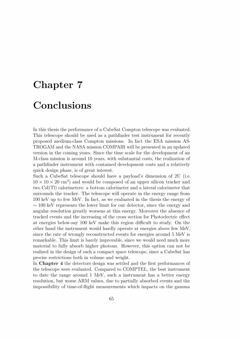
Chapter 7
Conclusions
In this thesis the performance of a CubeSat Compton telescope was evaluated.This telescope should be used as a pathfinder test instrument for recentlyproposed medium-class Compton missions. In fact the ESA mission AS-TROGAM and the NASA mission COMPAIR will be presented in an updatedversion in the coming years. Since the time scale for the development of anM-class mission is around 10 years, with substantial costs, the realization ofa pathfinder instrument with contained development costs and a relativelyquick design phase, is of great interest.Such a CubeSat telescope should have a payload’s dimension of 2U (i.e.10 × 10 × 20 cm3) and would be composed of an upper silicon tracker andtwo CsI(Tl) calorimeters: a bottom calorimeter and a lateral calorimeter thatsurrounds the tracker. The telescope will operate in the energy range from100 keV up to few MeV. In fact, as we evaluated in the thesis the energy of∼ 100 keV represents the lower limit for our detector, since the energy andangular resolution greatly worsens at this energy. Moreover the absence oftracked events and the increasing of the cross section for Photoelectric effectat energies below-say 100 keV make this region difficult to study. On theother hand the instrument would hardly operate at energies above few MeV,since the rate of wrongly reconstructed events for energies around 5 MeV isremarkable. This limit is barely improvable, since we would need much morematerial to fully absorb higher photons. However, this option can not berealized in the design of such a compact space telescope, since a CubeSat hasprecise restrictions both in volume and weight.In Chapter 4 the detectors design was settled and the first performances ofthe telescope were evaluated. Compared to COMPTEL, the best instrumentto date the range around 1 MeV, such a instrument has a better energyresolution, but worse ARM values, due to partially absorbed events and theimpossibility of time-of-flight measurements which impacts on the gamma
65

66 CHAPTER 7. CONCLUSIONS
background rates. In Chapter 5 further analyses are presented, selectingand dividing the total events in different classes (e.g. tracked and not trackedevents). Many simulations were performed, in order to optimize the detectordesign and validate the characteristics settled both for the tracker geometryand the read-out electronics (e.g. number of tracker layers, silicon strip pitch,noise etc.). Simultaneously a similar work was performed for the calorimeteroptimization (see [1]) and a final design of the telescope was settled.Finally, in Chapter 6 the first estimation of the telescope continuum sensi-tivity is computed, for different events classes and different energy intervals.At present the sensitivity estimated for the designed detector is worse thanthat achieved by COMPTEL. This is mostly due to the great presence ofalbedo background events. To avoid this problem two different solutions canbe possible. First of all we can consider an higher orbit for our detector. Inour design the telescope will orbit in Low Earth Orbit (LEO), at a nominalheight of 450− 500 km. An higher orbit (e.g. High Earth Orbit, HEO) im-plies a smaller rate of albedo background events, but the background due topassive material activation becomes remarkable. This is a great complication,since material activation produces events inside the anticoincidence shield.Moreover an higher orbit also implies an increase of the launch costs and moredifficulties in data communications, making this solution hardly realizable,especially for a small CubeSat mission.The other possibility is to implement new algorithms and perform significantquality cuts in order to drastically differentiate background and wronglyreconstructed events, from properly reconstructed events. In this way, in thenext future there is the actual opportunity to greatly improve the estimationpresented in this thesis and to obtain a sensitivity better than the one achievedby COMPTEL.

Appendix A
Quality cuts
From our analysis the best configuration designed is the lateral calorimeter 1configuration defined in Chapter 4. A further step is to find good criteria todifferentiate poorly reconstructed events from properly reconstructed events.As we have seen, this is especially important at lower energies (∼ 100keV) andat higher energies (≥ 1000 keV) where the ARM spectra exhibit considerableleft and right tails, due to incompletely absorbed particles. To achieve thisscope some quality cuts were performed. These cuts were performed withoutconsidering background events, since they were meant only to understandthe topology of wrongly reconstructed events. Thus, the obtained results arestill preliminary; therefore they are included in an appendix and not in themain body of the thesis. However they are very important in order to reacha general understanding of how the telescope works, and will be useful todevelop more complex and effective cuts in the future.We first looked for possible anomalies in the events reconstruction consideringthe Compton quality factor given back in the output of our simulations. TheCompton quality factor is computed from the Spearman Rank correlationcoefficient to find the most probable combination of the paths the particlesmight have taken in the interaction with the telescope detectors (more detailscan be found in [30]). Although a Compton quality factor cut would be themost logical choice, it does not improve very much the ARM spectrum. Itcan be seen in Figure A.1 where we kept the 80% events with best qualityfactor values. Therefore we looked for other possible cuts involving otherkinematics variables as cuts in the scattering angles and in sequence length(i.e. the number of hits in the reconstruction sequence).
67
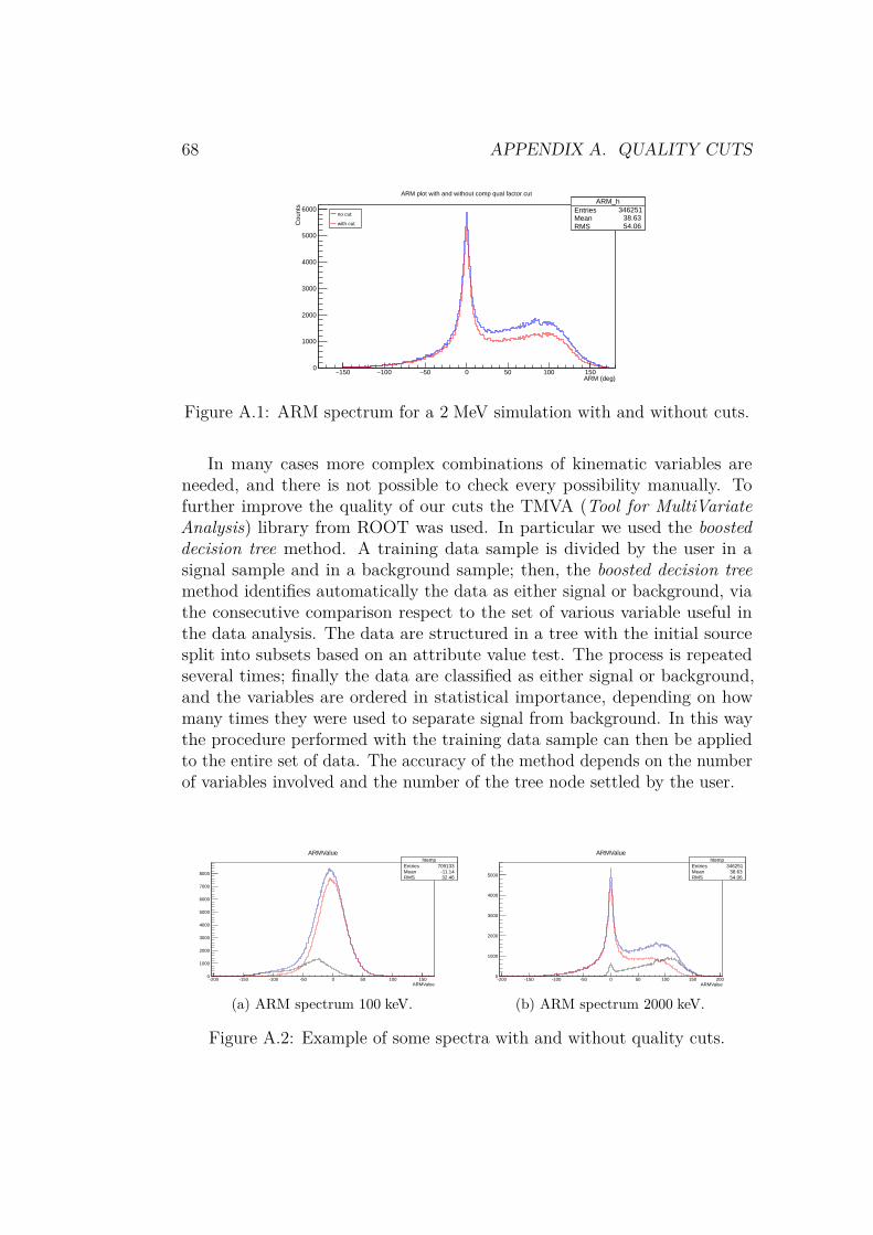
68 APPENDIX A. QUALITY CUTS
ARM_hEntries 346251Mean 38.63RMS 54.06
ARM (deg)150− 100− 50− 0 50 100 150
Cou
nts
0
1000
2000
3000
4000
5000
6000ARM_h
Entries 346251Mean 38.63RMS 54.06
no cut
with cut
ARM plot with and without comp qual factor cut
Figure A.1: ARM spectrum for a 2 MeV simulation with and without cuts.
In many cases more complex combinations of kinematic variables areneeded, and there is not possible to check every possibility manually. Tofurther improve the quality of our cuts the TMVA (Tool for MultiVariateAnalysis) library from ROOT was used. In particular we used the boosteddecision tree method. A training data sample is divided by the user in asignal sample and in a background sample; then, the boosted decision treemethod identifies automatically the data as either signal or background, viathe consecutive comparison respect to the set of various variable useful inthe data analysis. The data are structured in a tree with the initial sourcesplit into subsets based on an attribute value test. The process is repeatedseveral times; finally the data are classified as either signal or background,and the variables are ordered in statistical importance, depending on howmany times they were used to separate signal from background. In this waythe procedure performed with the training data sample can then be appliedto the entire set of data. The accuracy of the method depends on the numberof variables involved and the number of the tree node settled by the user.
htempEntries 709133Mean -11.14RMS 32.46
ARMValue-200 -150 -100 -50 0 50 100 150
0
1000
2000
3000
4000
5000
6000
7000
8000
htempEntries 709133Mean -11.14RMS 32.46
ARMValue
(a) ARM spectrum 100 keV.
htempEntries 346251Mean 38.63RMS 54.06
ARMValue-200 -150 -100 -50 0 50 100 150 200
0
1000
2000
3000
4000
5000
htempEntries 346251Mean 38.63RMS 54.06
ARMValue
(b) ARM spectrum 2000 keV.
Figure A.2: Example of some spectra with and without quality cuts.

69
Firstly we performed TMVA cuts on single energy spectra and secondly weapplied the TMVA procedure to a total spectrum with a final training samplecomposed of multiple energies data (in order to obtain final cuts independenton the energy of the sample). The signal was defined as all the events with−20 ≤ ARM ≤ 20 (central peak), while the remaining events are classifiedas background. Moreover the number of nodes was set to 4, that is a quitesimple and unrealistic number for definitive quality cuts, but in this phase wewant to manually reconstruct the trees in order to understand the variablesimportance in the procedure. With every single cut a fraction of 20− 25% ofthe total events was discarded and some examples are presented in Figure A.2:the histogram in blue represents the total data, in black the rejected data areplotted, and in red are represented the data after quality cuts. As we can seeat the energy of 100 keV a great fraction of biased events is rejected, while atthe energy of 2 MeV we can observe the decreasing of the events in the righttail.As shown in Figure A.3 with the cuts performed some parameters, such asthe ARM containment intervals and the ARM bias greatly improve.
Energy (keV)210 310
AR
M F
WH
M (
deg)
10
15
20
25
30
35
40
45
50
55
ARM plot (comparison)
no cutsmanual cutsTMVA single cutsTMVA total cuts
(a) ARM FWHM.Energy (keV)
210 310
AR
M b
ias
(deg
)
6−
5−
4−
3−
2−
1−
0
ARM bias plot (comparison)
no cutsmanual cutsTMVA single cutsTMVA total cuts
(b) ARM bias.
Energy (keV)210 310
AR
M in
terv
al (
deg)
20
30
40
50
60
70
80
90
100
110
ARM 68% intervals plot (comparison)
no cutsmanual cutsTMVA single cutsTMVA total cuts
(c) ARM 68% interval.Energy (keV)
210 310
AR
M in
terv
al (
deg)
100
120
140
160
180
200
ARM 95% intervals plot (comparison)
no cutsmanual cutsTMVA single cutsTMVA total cuts
(d) ARM 95% interval.
Figure A.3: Results after quality cuts.

70 APPENDIX A. QUALITY CUTS

Appendix B
Tracker optimization plots
Layers number simulations
Energy (keV)200 400 600 800 1000 1200 1400 1600 1800 2000
)2E
ffect
ive
Are
a (c
m
0
0.5
1
1.5
2
2.5
3
3.5
Effective Area for different events classes
Tracked + Bottom Calorimeter
Tracked + Lateral Calorimeter
Hit Tracker + Bottom Calorimeter
Hit Tracker + Lateral Calorimeter
(a) Effective area.Energy (keV)
200 400 600 800 1000 1200 1400 1600 1800 2000
Ene
rgy
reso
lutio
n (%
)
5
10
15
20
25
Energy resolution for different events classes
Tracked + Bottom Calorimeter
Tracked + Lateral Calorimeter
Hit Tracker + Botton Calorimeter
Hit Tracker + Lateral Calorimeter
(b) Energy resolution.
Energy (keV)200 400 600 800 1000 1200 1400 1600 1800 2000
AR
M F
WH
M (
deg)
20
30
40
50
60
70
ARM for different events classes
Tracked + Bottom Calorimeter
Tracked + Lateral Calorimeter
Hit Tracker + Bottom Calorimeter
Hit Tracker + Lateral Calorimeter
(c) ARM FWHM.Energy (keV)
400 600 800 1000 1200 1400 1600 1800 2000
SP
D H
WH
M (
deg)
22
24
26
28
30
32
34
36
38
40
42
44
SPD for different events classes
Tracked + Bottom Calorimeter
Tracked + Lateral Calorimeter
(d) SPD HWHM.
Figure B.1: Parameters estimated for the configuration with 20 layers.
71

72 APPENDIX B. TRACKER OPTIMIZATION PLOTS
Energy (keV)200 400 600 800 1000 1200 1400 1600 1800 2000
)2E
ffect
ive
Are
a (c
m
0
1
2
3
4
5
Effective Area for different events classes
Tracked + Bottom Calorimeter
Tracked + Lateral Calorimeter
Hit Tracker + Bottom Calorimeter
Hit Tracker + Lateral Calorimeter
(a) Effective area.Energy (keV)
200 400 600 800 1000 1200 1400 1600 1800 2000
Ene
rgy
reso
lutio
n (%
)
5
10
15
20
25
Energy resolution for different events classes
Tracked + Bottom Calorimeter
Tracked + Lateral Calorimeter
Hit Tracker + Botton Calorimeter
Hit Tracker + Lateral Calorimeter
(b) Energy resolution.
Energy (keV)200 400 600 800 1000 1200 1400 1600 1800 2000
AR
M F
WH
M (
deg)
20
30
40
50
60
70
ARM for different events classes
Tracked + Bottom Calorimeter
Tracked + Lateral Calorimeter
Hit Tracker + Bottom Calorimeter
Hit Tracker + Lateral Calorimeter
(c) ARM FWHM.Energy (keV)
400 600 800 1000 1200 1400 1600 1800 2000
SP
D H
WH
M (
deg)
25
30
35
40
45
SPD for different events classes
Tracked + Bottom Calorimeter
Tracked + Lateral Calorimeter
(d) SPD HWHM.
Figure B.2: Parameters estimated for the configuration with 25 layers.

73
Layers thickness simulations
Energy (keV)200 400 600 800 1000 1200 1400 1600 1800 2000
)2E
ffect
ive
Are
a (c
m
0
1
2
3
4
5
Effective Area for different events classes
Tracked + Bottom Calorimeter
Tracked + Lateral Calorimeter
Hit Tracker + Bottom Calorimeter
Hit Tracker + Lateral Calorimeter
(a) Effective area.Energy (keV)
200 400 600 800 1000 1200 1400 1600 1800 2000
Ene
rgy
reso
lutio
n (%
)
5
10
15
20
25
Energy resolution for different events classes
Tracked + Bottom Calorimeter
Tracked + Lateral Calorimeter
Hit Tracker + Botton Calorimeter
Hit Tracker + Lateral Calorimeter
(b) Energy resolution.
Energy (keV)200 400 600 800 1000 1200 1400 1600 1800 2000
AR
M F
WH
M (
deg)
10
20
30
40
50
60
70
ARM for different events classes
Tracked + Bottom Calorimeter
Tracked + Lateral Calorimeter
Hit Tracker + Bottom Calorimeter
Hit Tracker + Lateral Calorimeter
(c) ARM FWHM.Energy (keV)
400 600 800 1000 1200 1400 1600 1800 2000
SP
D H
WH
M (
deg)
20
25
30
35
40
SPD for different events classes
Tracked + Bottom Calorimeter
Tracked + Lateral Calorimeter
(d) SPD HWHM.
Figure B.3: Parameters estimated for the configuration with 400 µm layerthickness.
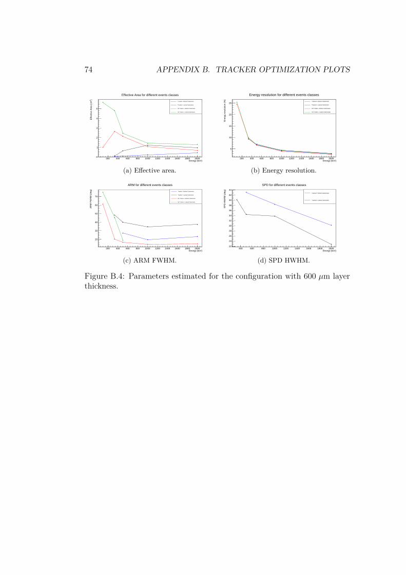
74 APPENDIX B. TRACKER OPTIMIZATION PLOTS
Energy (keV)200 400 600 800 1000 1200 1400 1600 1800 2000
)2E
ffect
ive
Are
a (c
m
0
1
2
3
4
5
Effective Area for different events classes
Tracked + Bottom Calorimeter
Tracked + Lateral Calorimeter
Hit Tracker + Bottom Calorimeter
Hit Tracker + Lateral Calorimeter
(a) Effective area.Energy (keV)
200 400 600 800 1000 1200 1400 1600 1800 2000
Ene
rgy
reso
lutio
n (%
)
5
10
15
20
25
Energy resolution for different events classes
Tracked + Bottom Calorimeter
Tracked + Lateral Calorimeter
Hit Tracker + Botton Calorimeter
Hit Tracker + Lateral Calorimeter
(b) Energy resolution.
Energy (keV)200 400 600 800 1000 1200 1400 1600 1800 2000
AR
M F
WH
M (
deg)
20
30
40
50
60
70
ARM for different events classes
Tracked + Bottom Calorimeter
Tracked + Lateral Calorimeter
Hit Tracker + Bottom Calorimeter
Hit Tracker + Lateral Calorimeter
(c) ARM FWHM.Energy (keV)
400 600 800 1000 1200 1400 1600 1800 2000
SP
D H
WH
M (
deg)
22
24
26
28
30
32
34
36
38
40
42
44
SPD for different events classes
Tracked + Bottom Calorimeter
Tracked + Lateral Calorimeter
(d) SPD HWHM.
Figure B.4: Parameters estimated for the configuration with 600 µm layerthickness.

75
Strip pitch simulations
Energy (keV)200 400 600 800 1000 1200 1400 1600 1800 2000
)2E
ffect
ive
Are
a (c
m
0
1
2
3
4
5
6
Effective Area for different events classes
Tracked + Bottom Calorimeter
Tracked + Lateral Calorimeter
Hit Tracker + Bottom Calorimeter
Hit Tracker + Lateral Calorimeter
(a) Effective area.Energy (keV)
200 400 600 800 1000 1200 1400 1600 1800 2000
Ene
rgy
reso
lutio
n (%
)
5
10
15
20
25
Energy resolution for different events classes
Tracked + Bottom Calorimeter
Tracked + Lateral Calorimeter
Hit Tracker + Botton Calorimeter
Hit Tracker + Lateral Calorimeter
(b) Energy resolution.
Energy (keV)200 400 600 800 1000 1200 1400 1600 1800 2000
AR
M F
WH
M (
deg)
10
20
30
40
50
60
70
ARM for different events classes
Tracked + Bottom Calorimeter
Tracked + Lateral Calorimeter
Hit Tracker + Bottom Calorimeter
Hit Tracker + Lateral Calorimeter
(c) ARM FWHM.Energy (keV)
400 600 800 1000 1200 1400 1600 1800 2000
SP
D H
WH
M (
deg)
22
24
26
28
30
32
34
36
38
40
SPD for different events classes
Tracked + Bottom Calorimeter
Tracked + Lateral Calorimeter
(d) SPD HWHM.
Figure B.5: Parameters estimated for the configuration with a strip pitch of50 µm.

76 APPENDIX B. TRACKER OPTIMIZATION PLOTS
Energy (keV)200 400 600 800 1000 1200 1400 1600 1800 2000
)2E
ffect
ive
Are
a (c
m
0
1
2
3
4
5
6
Effective Area for different events classes
Tracked + Bottom Calorimeter
Tracked + Lateral Calorimeter
Hit Tracker + Bottom Calorimeter
Hit Tracker + Lateral Calorimeter
(a) Effective area.Energy (keV)
200 400 600 800 1000 1200 1400 1600 1800 2000
Ene
rgy
reso
lutio
n (%
)
5
10
15
20
25
Energy resolution for different events classes
Tracked + Bottom Calorimeter
Tracked + Lateral Calorimeter
Hit Tracker + Botton Calorimeter
Hit Tracker + Lateral Calorimeter
(b) Energy resolution.
Energy (keV)200 400 600 800 1000 1200 1400 1600 1800 2000
AR
M F
WH
M (
deg)
20
30
40
50
60
70
ARM for different events classes
Tracked + Bottom Calorimeter
Tracked + Lateral Calorimeter
Hit Tracker + Bottom Calorimeter
Hit Tracker + Lateral Calorimeter
(c) ARM FWHM.Energy (keV)
400 600 800 1000 1200 1400 1600 1800 2000
SP
D H
WH
M (
deg)
25
30
35
40
45
SPD for different events classes
Tracked + Bottom Calorimeter
Tracked + Lateral Calorimeter
(d) SPD HWHM.
Figure B.6: Parameters estimated for the configuration with a strip pitch of300 µm.
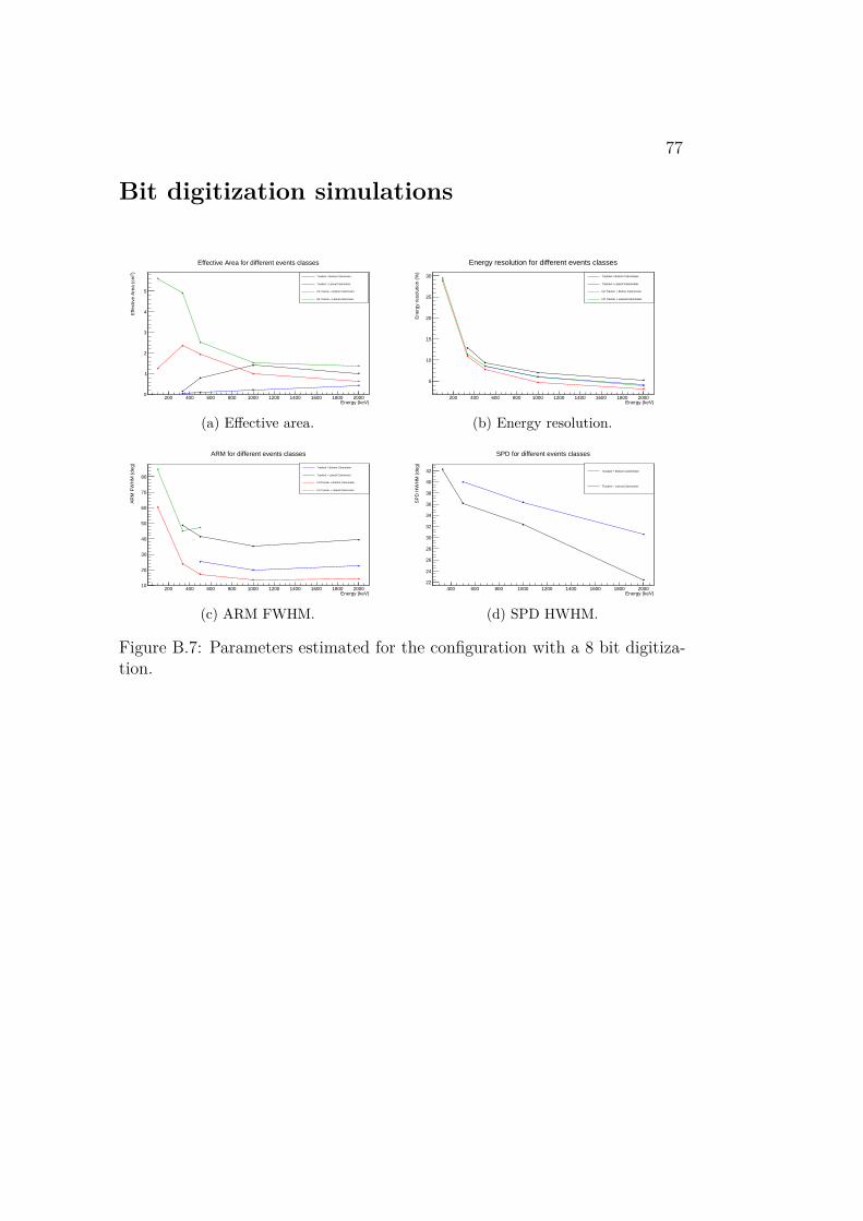
77
Bit digitization simulations
Energy (keV)200 400 600 800 1000 1200 1400 1600 1800 2000
)2E
ffect
ive
Are
a (c
m
0
1
2
3
4
5
Effective Area for different events classes
Tracked + Bottom Calorimeter
Tracked + Lateral Calorimeter
Hit Tracker + Bottom Calorimeter
Hit Tracker + Lateral Calorimeter
(a) Effective area.Energy (keV)
200 400 600 800 1000 1200 1400 1600 1800 2000
Ene
rgy
reso
lutio
n (%
)
5
10
15
20
25
30
Energy resolution for different events classes
Tracked + Bottom Calorimeter
Tracked + Lateral Calorimeter
Hit Tracker + Botton Calorimeter
Hit Tracker + Lateral Calorimeter
(b) Energy resolution.
Energy (keV)200 400 600 800 1000 1200 1400 1600 1800 2000
AR
M F
WH
M (
deg)
10
20
30
40
50
60
70
80
ARM for different events classes
Tracked + Bottom Calorimeter
Tracked + Lateral Calorimeter
Hit Tracker + Bottom Calorimeter
Hit Tracker + Lateral Calorimeter
(c) ARM FWHM.Energy (keV)
400 600 800 1000 1200 1400 1600 1800 2000
SP
D H
WH
M (
deg)
22
24
26
28
30
32
34
36
38
40
42
SPD for different events classes
Tracked + Bottom Calorimeter
Tracked + Lateral Calorimeter
(d) SPD HWHM.
Figure B.7: Parameters estimated for the configuration with a 8 bit digitiza-tion.
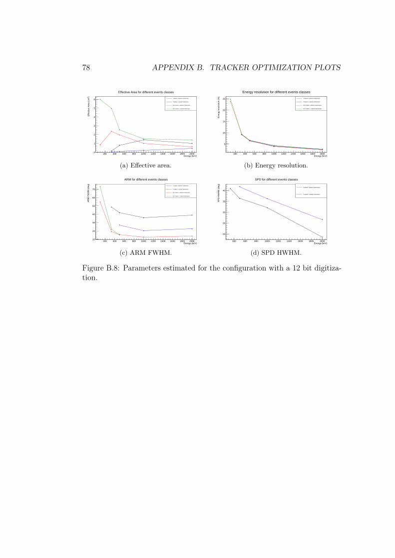
78 APPENDIX B. TRACKER OPTIMIZATION PLOTS
Energy (keV)200 400 600 800 1000 1200 1400 1600 1800 2000
)2E
ffect
ive
Are
a (c
m
0
1
2
3
4
5
6
Effective Area for different events classes
Tracked + Bottom Calorimeter
Tracked + Lateral Calorimeter
Hit Tracker + Bottom Calorimeter
Hit Tracker + Lateral Calorimeter
(a) Effective area.Energy (keV)
200 400 600 800 1000 1200 1400 1600 1800 2000
Ene
rgy
reso
lutio
n (%
)
5
10
15
20
25
Energy resolution for different events classes
Tracked + Bottom Calorimeter
Tracked + Lateral Calorimeter
Hit Tracker + Botton Calorimeter
Hit Tracker + Lateral Calorimeter
(b) Energy resolution.
Energy (keV)200 400 600 800 1000 1200 1400 1600 1800 2000
AR
M F
WH
M (
deg)
10
20
30
40
50
60
70
ARM for different events classes
Tracked + Bottom Calorimeter
Tracked + Lateral Calorimeter
Hit Tracker + Bottom Calorimeter
Hit Tracker + Lateral Calorimeter
(c) ARM FWHM.Energy (keV)
400 600 800 1000 1200 1400 1600 1800 2000
SP
D H
WH
M (
deg)
20
25
30
35
40
SPD for different events classes
Tracked + Bottom Calorimeter
Tracked + Lateral Calorimeter
(d) SPD HWHM.
Figure B.8: Parameters estimated for the configuration with a 12 bit digitiza-tion.

79
Equivalent Noise Charge simulations
Energy (keV)200 400 600 800 1000 1200 1400 1600 1800 2000
)2E
ffect
ive
Are
a (c
m
0
1
2
3
4
5
6
Effective Area for different events classes
Tracked + Bottom Calorimeter
Tracked + Lateral Calorimeter
Hit Tracker + Bottom Calorimeter
Hit Tracker + Lateral Calorimeter
(a) Effective area.Energy (keV)
200 400 600 800 1000 1200 1400 1600 1800 2000
Ene
rgy
reso
lutio
n (%
)
2
4
6
8
10
12
14
16
18
20
22
24
Energy resolution for different events classes
Tracked + Bottom Calorimeter
Tracked + Lateral Calorimeter
Hit Tracker + Botton Calorimeter
Hit Tracker + Lateral Calorimeter
(b) Energy resolution.
Energy (keV)200 400 600 800 1000 1200 1400 1600 1800 2000
AR
M F
WH
M (
deg)
10
20
30
40
50
60
ARM for different events classes
Tracked + Bottom Calorimeter
Tracked + Lateral Calorimeter
Hit Tracker + Bottom Calorimeter
Hit Tracker + Lateral Calorimeter
(c) ARM FWHM.Energy (keV)
400 600 800 1000 1200 1400 1600 1800 2000
SP
D H
WH
M (
deg)
20
25
30
35
40
SPD for different events classes
Tracked + Bottom Calorimeter
Tracked + Lateral Calorimeter
(d) SPD HWHM.
Figure B.9: Parameters estimated for the configuration with a 600 e− ENC.

80 APPENDIX B. TRACKER OPTIMIZATION PLOTS
Energy (keV)200 400 600 800 1000 1200 1400 1600 1800 2000
)2E
ffect
ive
Are
a (c
m
0
1
2
3
4
5
6
Effective Area for different events classes
Tracked + Bottom Calorimeter
Tracked + Lateral Calorimeter
Hit Tracker + Bottom Calorimeter
Hit Tracker + Lateral Calorimeter
(a) Effective area.Energy (keV)
200 400 600 800 1000 1200 1400 1600 1800 2000
Ene
rgy
reso
lutio
n (%
)
5
10
15
20
25
30
Energy resolution for different events classes
Tracked + Bottom Calorimeter
Tracked + Lateral Calorimeter
Hit Tracker + Botton Calorimeter
Hit Tracker + Lateral Calorimeter
(b) Energy resolution.
Energy (keV)200 400 600 800 1000 1200 1400 1600 1800 2000
AR
M F
WH
M (
deg)
20
30
40
50
60
70
80
ARM for different events classes
Tracked + Bottom Calorimeter
Tracked + Lateral Calorimeter
Hit Tracker + Bottom Calorimeter
Hit Tracker + Lateral Calorimeter
(c) ARM FWHM.Energy (keV)
400 600 800 1000 1200 1400 1600 1800 2000
SP
D H
WH
M (
deg)
22
24
26
28
30
32
34
36
38
40
42
SPD for different events classes
Tracked + Bottom Calorimeter
Tracked + Lateral Calorimeter
(d) SPD HWHM.
Figure B.10: Parameters estimated for the configuration with a 2400 e− ENC.

Appendix C
Abbreviations and notationsused
AbbreviationsSN SupernovaGRB Gamma-ray BurstAGN Active Galactic NucleusSED Spectral Energy DistributionENC Equivalent Noise ChargeARM Angular Resolution MeasurementSPD Scatter Plane DeviationPSF Point Spread FunctionEGB Extragalactic Gamma-ray Background
NotationsEi Energy of the incident gamma-rayEe Energy of the recoil electronEg Energy of the scattered gamma-rayϕ Compton scatter angle of gamma-rayε Scatter angle of the recoil electronϑ Total scatter angle~ei Direction of the incident gamma-ray~ee Direction of the recoil electron~eg Direction of the scattered gamma-ray
81

82 APPENDIX C. ABBREVIATIONS AND NOTATIONS USED
Fz SensitivityAeff Effective AreaTeff Observation time

Ringraziamenti
Sono molte le persone che vorrei ringraziare per aver reso possibile il comple-tamento di questo lavoro. Innanzitutto, ringrazio il Dottor Riccardo Rando eil Professor Denis Bastieri per la disponibilità e per la pazienza dimostrata,per gli spunti e i consigli forniti, non solo nel corso di questo lavoro di TesiMagistrale, ma anche in quello di Tesi Triennale. Ringrazio poi FrancescoBerlato, con cui ho callaborato all’interno di questo progetto, e con il qualeho condiviso opinioni, dubbi e molti segmentation faults.Ovviamente, i ringraziamenti devono essere estesi anche a tutte quelle per-sone che mi hanno aiutato nell’intero arco del percorso universitario e oltre.Innanzitutto alla mia famiglia, soprattutto a mia madre, che mi ha sempresostenuto. Ringrazio poi tutti gli amici e colleghi Nicolò, Marco, Chiara,Daniele, Piero e Alessandro, con i quali ho condiviso lo stress e l’ansia permolti esami (anche se sarebbe meglio dire: che hanno sopportato il mio stresse la mia ansia), ma anche aperitivi molesti, serate nerd, canzoni trash emolti altri bei e petalosi momenti. Infatti, come disse una volta un "valorosocombattente": "Ragazzi, sono dei vostri!".
83

84 APPENDIX C. ABBREVIATIONS AND NOTATIONS USED

Bibliography
[1] F. Berlato. “Design and optimization around 1 MeV of a calorimeter fora CubeSat Mission”. Master Thesis. Università degli Studi di Padova,2016.
[2] M. Böettcher. “Modeling the emission processes in blazars”. In: Astro-physics and Space Science 309 (2007).
[3] R. Diehl. “The COMPTEL experiment on the NASA Gamma-rayObservatory”. In: Space Science Reviews 49 (1988).
[4] A. A. Abdo et al. “Fermi-LAT Observations of Markarian 421: theMissing Piece of its Spectral Energy Distribution”. In: The AstrophysicalJournal 736(2) (2011).
[5] A. C. Zoglauer et al. “Cosima – the Cosmic Simulator of MEGAlib”. In:IEEE Nuclear Science Symposium conference record. Nuclear ScienceSymposium (2009).
[6] A. C. Zoglauer et al. “MEGAlib-Simulation and Data Analysis forLow-to-medium-energy Gamma-ray Telescopes”. In: Proceedings of theSPIE 7011 (2008).
[7] A. C. Zoglauer et al. “MEGAlib — The Medium Energy Gamma-rayAstronomy Library”. In: New Astronomy Reviews 50(7) (2006).
[8] A. Hoecker et al. “TMVA 4: Toolkit for Multivariate Data Analysiswith ROOT, Users Guide”. In: arXiv:physics/0703039 (2013).
[9] A.A. Moiseev et al. “Compton-Pair Production Space Telescope (Com-Pair) for MeV Gamma-ray Astronomy”. In: arXiv:1508.07349 (2015).
[10] H. Odaka et al. “High-resolution Compton cameras based on Si/CdTedouble-sided strip detectors”. In: Nuclear Instruments and Methods inPhysics Research, section A (2012).
[11] M. Böettcher et al. “Leptonic and Hadronic Modeling of Fermi-DetectedBlazars”. In: The Astrophysical Journal 768 (2013).
85

86 BIBLIOGRAPHY
[12] P. A. Milne et al. “Supernova Science with an Advanced ComptonTelescope”. In: arXiv:astro-ph/0012078 (2000).
[13] P. Bloser et al. “Development of Silicon Strip Detectors for a MediumEnergy Gamma-ray Telescope”. In: arXiv:astro-ph/0302500 (2003).
[14] S. Boggs et al. “Advanced Compton Telescope (ACT): witness to thefires of creation”. Proposal. 2005.
[15] V. Schönfelder et al. “Instrument description and performance ofthe Imaging Gamma-Ray Telescope COMPTEL aboard the Comp-ton Gamma-Ray Observatory”. In: Astrophysical Journal SupplementSeries 86 (1993).
[16] W. B. Atwood et al. “The Large Area Telescope on the Fermi Gamma-ray Space Telescope Mission”. In: The Astrophysical Journal 697 (2)(2009).
[17] ideas ASA, ed. VA64TA1 datasheet. 2004.[18] S. Cheenu Kappadath. “Measurement of the Cosmic Diffuse Gamma-
Ray Spectrum from 800 keV to 30 MeV”. PhD Thesis. University ofNew Hampshire, 1998.
[19] R. Marc Kippen. “The GEANT Low Energy Compton Scattering(GLECS) Package for use in Simulating Advanced Compton Telescopes”.In: New Astronomy Reviews 48 (2004).
[20] Glenn F. Knoll. Radiation Detection and Measurement. Ed. by JohnWiley and Sons Inc. 2010.
[21] V. Schönfelder. “Lessons learnt from COMPTEL for Future Telescopes”.In: New Astronomy Reviews (2003).
[22] V. Schönfelder and G. Kanbach. “Imaging through Compton scatter-ing and pair creation”. In: Observing Photons in Space: a guide toExperimental Space Astronomy (2013).
[23] Helmuth Spieler. Semiconductor Detector Systems. Ed. by Oxford Uni-versity Press. 2005.
[24] H. Tajima. Front-end Card Specification for VA64TA. 2007.[25] M. Tavani and V. Tatischeff. “ASTROGAM: Proposal for the ESA M4
Mission Programme”. Proposal. 2015.[26] C. M. Urry and P. Padovani. “Unified Schemes for Radio-Loud Active
Galactic Nuclei”. In: Astronomical Society of the Pacific 715 (1995).

BIBLIOGRAPHY 87
[27] M. Tavani V. Tatischeff. “The e-ASTROGAM gamma-ray space mis-sion”. In: Proc. SPIE 9905, Space Telescopes and Instrumentation 2016:Ultraviolat to Gamma Ray (2016).
[28] H. Voss. “Data Analysis with TMVA”. In: Seminar, Lausanne (2010).[29] A. C. Zoglauer. Cosima, a Cosmic Simulator for MEGAlib based on
Geant4. 2015.[30] A. C. Zoglauer. “First Light for the Next Generation of Compton
and Pair Telescopes”. PhD Thesis. Max Planck Institut für Extrater-restrische Physik, 2005.
[31] A. C. Zoglauer. Geomega, Geometry for MEGAlib. 2014.[32] A. C. Zoglauer. Mimrec, MEGAlib image reconstruction and more ...
2010.[33] A. C. Zoglauer. The MEGAlib software package. 2006.