universitÀ degli studi di perugia - infn.it universitÀ degli studi di perugia dipartimento...
TRANSCRIPT
UNIVERSITÀ DEGLI STUDI DI PERUGIA
Dipartimento d’Ingegneria
Corso di Laurea Magistrale in Ingegneria Meccanica
TESI DI LAUREA MAGISTRALE
The silicon strip modules of the outer tracker of the CMS
(Compact Muon Solenoid) experiment at LHC (Large Hadron
Collider): thermal studies
Relatori Candidato
Ing. Giorgio Baldinelli Cristiano Turrioni
Prof. Claudia Cecchi
Ing. Francesco Bianchi
Anno Accademico 2016/2017

“ Per tutti quelli
che continuano a lottare …”

I
SUMMARY
INTRODUCTION IV
THE LHC – LARGE HADRON COLLIDER 1
1.1 The Large Hadron Collider 1
1.2 Scientific Purposes 4
1.3 Discoveries and Social Impact 4
THE CMS – COMPACT MUON SOLENOID 8
2.1 General layout of the Experiment 8
2.2 The CMS Phase-2 Upgrade 9
2.3 The Interaction Point 10
2.4 The Tracker 10
2.5 The Electromagnetic Calorimeter 16
2.6 The Hadronic Calorimeter 16
2.7 The Superconducting Solenoid 17
2.8 The Muon System 17
THE 2S - 2 STRIPS MODULE OF THE OUTER SILICON
TRACKER IN CMS 19
3.1 Operating Fundamentals of Silicon Sensors 19
3.2 Components and General Layout of the Module 21
3.3 Cooling and Thermal Requirements 26
3.4 Module Assembly 29
II
HEAT TRANSFER ELEMENTS 34
4.1 Heat Exchange Mechanisms 34
4.2 Conduction Heat Transfer 35
4.3 Convection Heat Transfer 37
4.4 Thermal Radiation Heat Transfer 39
4.5 Treatment of Cavities 41
THE FINITE VOLUME METHOD 42
5.1 Equations of Conservation 42
5.2 Outline of the Finite Volume Method 44
5.3 Boundary Conditions 46
5.4 Sensitivity of the Solution to Errors 46
5.5 The Grid Convergence Index 48
FINITE VOLUME METHOD MODEL OF THE OUTER
TRACKER 2S MODULE 51
6.1 Introduction to the Software 51
6.2 Geometry of the Model 52
6.3 Meshing Procedure 56
6.4 Boundary Conditions 61
EXPERIMENTAL VALIDATION 67
7.1 Introduction to the Validation Procedure 67
7.2 The 2S Module for Tests 69
7.3 Peltier Cells 70
7.4 Heatsink System 74
7.5 Thermocouples 77

III
7.6 Test Number 1 80
7.7 Test Number 2 84
ANALYSIS OF RESULTS 89
8.1 Simulation N°1 compared with Test N°1 89
8.2 Simulation N°2 compared with Test N°2 98
8.3 Simulation of the module in operative conditions 103
FUTURE WORKS 107
9.1 Developments for the FVM model. 107
9.2 Developments for the test bench. 108
9.3 New tests for the module 109
CONCLUSIONS 112
REFERENCES 113
APPENDIX 116
IV
INTRODUCTION
“Somewhere, something incredible is waiting to be known.”
This thesis opens with a famous sentence attributed to Sharon Bagley, which sums up the
reasons that led to the work. One of the highest ambitions of the human beings is to question
about what happens in the world around it, trying to give answers to its insatiable desire of
knowledge. Curiosity and ambition have driven human society to dedicate a big part of its
resources to science, and the maximum expression of this is the creations of big research
organizations as the “Conseil européen pour la recherche nucléaire”, better known as CERN.
But science, over the years, has always gone hand in hand with technique. In this context
started the cooperation between the Italian National Institute for Nuclear Physics research
(INFN) and the Engineering Department of University of Perugia. The work described in
this thesis, born from the mentioned collaboration, is focused on the study of characteristics
of one of the components of a big particle detector that could help humans to know more
about what is happening in nature. This component, from here called “2S module” or just
“module”, is a silicon device that can detect the passage of subatomic particles: it is used in
atomic and nuclear physics. It is the basic part of the Outer Tracker of the Compact Muon
Solenoid (CMS) particle detector at the Large Hadron Collider (LHC) at CERN. The CMS
detector will be upgraded for the so called Phase2 of the LHC during the Long Shutdown 3
(LS3) scheduled to last from 2024 to mid 2016, and is now in the research and development
phase, in collaboration with thousand scientists and engineers from all over the world. A
particle detector is a device that can recognise particles that passing through it as well as
reconstruct the trajectories of some of them. In the first two chapters a description of CMS
will be presented, as well as the context in which it is inserted (i.e. the Large Hadron Collider
machine). CMS is already operative since 2008, but an upgrade is planned for the High
Luminosity phase. The 2S module, main component of the Outer Tracker, is part of this
upgrade. It is a silicon sensor which exploits the properties of doped semiconductors to
operate. Its description is given in chapter 3. In the context of particles detection, temperature
plays a key role because, in order to work, some sensors need a cooling system to make their
temperature low. The thermal studies conducted in this thesis are aimed at contributing to
fulfil this task. In order to describe the thermal behaviour of the module, a Finite Volume

V
Method model (FVM) has been implemented, starting from the study of its geometry and
operative conditions. To understand what is a FVM model and how it works, some basic
notions of heat transfer mechanism and numerical methods are described respectively in
chapters 4 and 5. In chapter 6, the procedure followed to create a computational model for
the module analysis is explained, and some results of simulations are reported. It is known
in the engineering sector that every numerical model needs an experimental validation to be
considered reliable. In order to obtain some experimental data to make a comparison with
the results of simulations, a test bench system has been constructed: its functioning is linked
to the needs of the module under study. The guidelines followed to build this system are
reported in chapter 7, as well as the experimental tests that have been executed. Comparison
of results obtained both from simulations and tests are shown in chapter 8, where once the
model has been validated, the simulation of the module under its operative conditions at
CMS is reported. During the process of study, some other tests and simulations have also
been planned for future works: these are included chapter 9.
1
Chapter 1
THE LHC – LARGE HADRON COLLIDER
1.1 The Large Hadron Collider
The Large Hadron Collider (LHC) is described [1] as the world newest and most powerful
particle accelerator for Physics research. It is designed to collide proton beams with a centre-
of-mass energy of 14 TeV (teraelectronvolts) and an unprecedented luminosity that is
1034cm-2s-1. It can also produce collisions between heavy (Pb) ions with an energy of 2.8
TeV per nucleon and a peak luminosity of 1027 cm-2s-1. It was built at CERN (European
Organization for Nuclear Research) between 1998 and 2008 (as described in [2]) in
collaboration with over 10.000 scientists and engineers from over 100 countries, as well as
hundreds of universities and laboratories. It is financed by European public funds and its
products belong to humanity. Its first physics run took place from March 2010 to early 2013
at an energy of 3.5 to 4 TeV per beam (7 to 8 TeV centre of mass energy), about 4 times the
previous world record for a collider. It is installed in a tunnel of 27 kilometres in
circumference, as deep as 175 metres beneath the France–Switzerland border near Geneva,
in a region between Geneva airport and the Jura mountains, originally excavated to build the
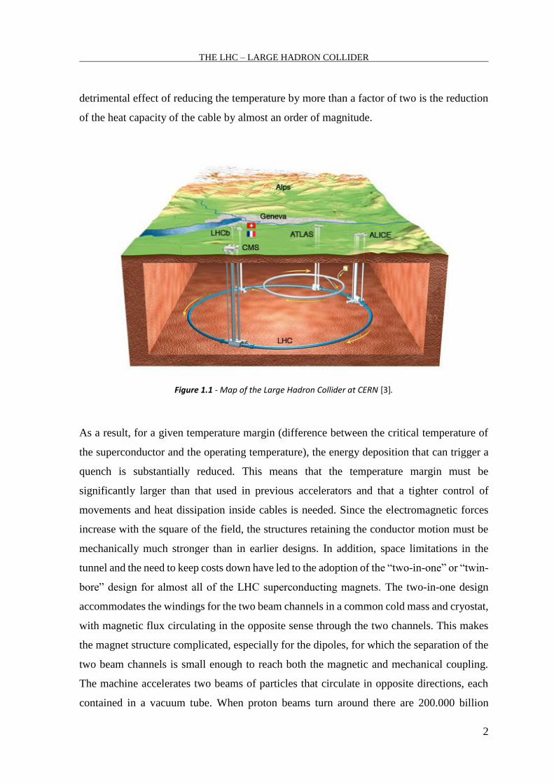
Large Electron-Positron Collider (LEP). A very simplified geographical map of the tunnel
is shown in Figure 1.1. The Large Hadron Collider relies on superconducting magnets that
are at the frontier of the present technology. Other large superconducting accelerators
(Tevatron-FNAL, HERA-DESY and RHICBNL) all use classical NbTi superconductors,
cooled by supercritical helium at temperatures slightly above 4.2 Kelvin (K), with fields
below or around 5 Tesla (T). LHC magnets work at 1.9 K (-271°C) which makes the machine
the coldest point in the known universe. At the same time the energy of the collisions
corresponds to a temperature of 1016 K. So we can both find very low temperatures and very
high temperatures in the same machine. The LHC magnet system, while still making use of
the well-proven technology based on NbTi Rutherford cables, cools the magnets to the
setpoint temperature using superfluid helium, and operates at fields above 8 T. One
THE LHC – LARGE HADRON COLLIDER
2
detrimental effect of reducing the temperature by more than a factor of two is the reduction
of the heat capacity of the cable by almost an order of magnitude.
Figure 1.1 - Map of the Large Hadron Collider at CERN [3].
As a result, for a given temperature margin (difference between the critical temperature of
the superconductor and the operating temperature), the energy deposition that can trigger a
quench is substantially reduced. This means that the temperature margin must be
significantly larger than that used in previous accelerators and that a tighter control of
movements and heat dissipation inside cables is needed. Since the electromagnetic forces
increase with the square of the field, the structures retaining the conductor motion must be
mechanically much stronger than in earlier designs. In addition, space limitations in the
tunnel and the need to keep costs down have led to the adoption of the “two-in-one” or “twin-
bore” design for almost all of the LHC superconducting magnets. The two-in-one design
accommodates the windings for the two beam channels in a common cold mass and cryostat,
with magnetic flux circulating in the opposite sense through the two channels. This makes
the magnet structure complicated, especially for the dipoles, for which the separation of the
two beam channels is small enough to reach both the magnetic and mechanical coupling.
The machine accelerates two beams of particles that circulate in opposite directions, each
contained in a vacuum tube. When proton beams turn around there are 200.000 billion
THE LHC – LARGE HADRON COLLIDER
3
protons in each beam and these beams collide 40 million times per second. These collisions
occur at four points along the orbit, in correspondence with caverns where the tunnel widens
to make space for large experimental rooms. These stations include the four main particle
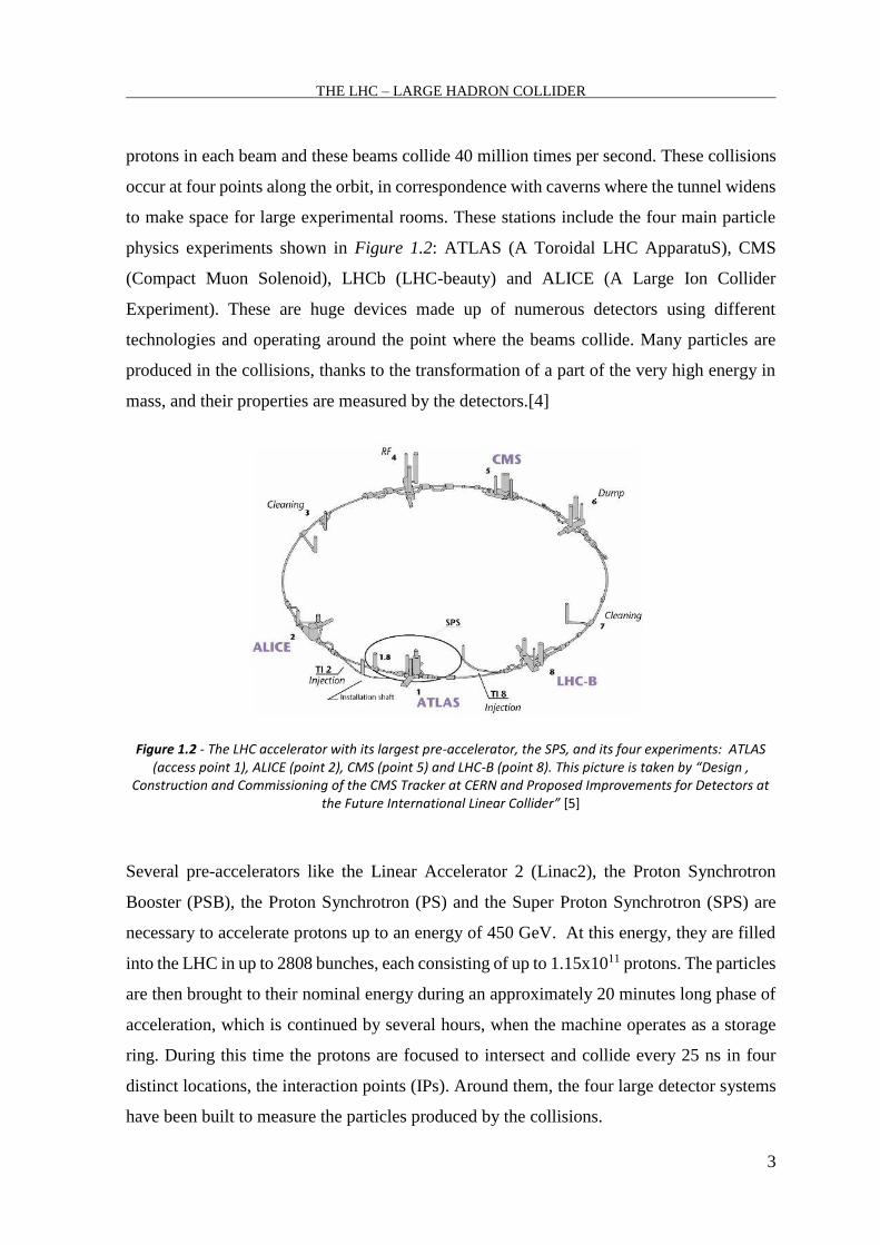
physics experiments shown in Figure 1.2: ATLAS (A Toroidal LHC ApparatuS), CMS
(Compact Muon Solenoid), LHCb (LHC-beauty) and ALICE (A Large Ion Collider
Experiment). These are huge devices made up of numerous detectors using different
technologies and operating around the point where the beams collide. Many particles are
produced in the collisions, thanks to the transformation of a part of the very high energy in
mass, and their properties are measured by the detectors.[4]
Figure 1.2 - The LHC accelerator with its largest pre-accelerator, the SPS, and its four experiments: ATLAS (access point 1), ALICE (point 2), CMS (point 5) and LHC-B (point 8). This picture is taken by “Design ,
Construction and Commissioning of the CMS Tracker at CERN and Proposed Improvements for Detectors at the Future International Linear Collider” [5]
Several pre-accelerators like the Linear Accelerator 2 (Linac2), the Proton Synchrotron
Booster (PSB), the Proton Synchrotron (PS) and the Super Proton Synchrotron (SPS) are
necessary to accelerate protons up to an energy of 450 GeV. At this energy, they are filled
into the LHC in up to 2808 bunches, each consisting of up to 1.15x10¹¹ protons. The particles
are then brought to their nominal energy during an approximately 20 minutes long phase of
acceleration, which is continued by several hours, when the machine operates as a storage
ring. During this time the protons are focused to intersect and collide every 25 ns in four
distinct locations, the interaction points (IPs). Around them, the four large detector systems
have been built to measure the particles produced by the collisions.
THE LHC – LARGE HADRON COLLIDER
4
1.2 Scientific Purposes
The main goal of LHC was is to help answering some of the fundamental open questions in
physics, concerning the basic laws governing the interactions and forces among the
elementary objects, the deep structure of space and time, and in particular the interrelation
between quantum mechanics and general relativity. LHC allows scientists to study the
fundamental constituents of matter, and then to obtain information on the structure of the
universe. The study of the infinitely small is strictly related to the infinitely large. The most
discussed questions are about supersymmetry, one of the possible extension of the Standard
Model, extra dimensions, Dark Matter and the generation mechanism of the property "mass"
of the elementary particles. There are also other open questions that may be explored using
high-energy particle collisions: for example, it is already known that electromagnetism and
the weak nuclear force are different manifestations of a single force called the electroweak
force. The LHC may clarify whether the electroweak force and the strong nuclear force are
similarly just different manifestations of one universal unified force, as predicted by various
Grand Unification Theories. Moreover, scientists would like to answer the question about
why is the fourth fundamental force (gravity) so many orders of magnitude weaker than the
other three fundamental forces. Furthermore, there are also many other questions, such as:
are there additional sources of quark flavour mixing, beyond those already present within
the Standard Model? Why are there apparent violations of the symmetry between matter and
antimatter? What are the nature and properties of quark–gluon plasma thought to have
existed in the early universe and in certain compact and strange astronomical objects today?
This will be investigated by heavy ion collisions, mainly by the ALICE experiment, but also
in CMS, ATLAS and LHCb. First observed in 2010, findings published in 2012 confirmed
the phenomenon of jet quenching in heavy-ion collisions.
1.3 Discoveries and Social Impact
Alongside the previous questions, which are the engine of scientific research carried out at
CERN, over the years there have been also numerous scientific discoveries of considerable
importance. The first relevant physics results from the Large Hadron Collider, involving 284
collisions which took place in the ALICE detector, were reported on 15 December 2009.
THE LHC – LARGE HADRON COLLIDER
5
After the first year of data collection, the LHC experimental collaborations started to release
their preliminary results concerning searches for new physics beyond the Standard Model in
proton-proton collisions. As a result, bounds were set on the allowed parameter space of
various extensions of the Standard Model, such as models with large extra dimensions,
constrained versions of the Minimal Supersymmetric Standard Model, and others. On 24
May 2011, it was reported that quark–gluon plasma (the densest matter thought to exist
besides black holes) had been created in the LHC. Between July and August 2011, results of
searches for the Higgs boson and for exotic particles, based on the data collected during the
first half of the 2011 run, were presented in conferences in Grenoble and Mumbai. In the
latter conference it was reported that, despite hints of a Higgs signal in earlier data, ATLAS
and CMS exclude with 95% confidence level (using the CLs method) the existence of a
Higgs boson with the properties predicted by the Standard Model over most of the mass
region between 145 and 466 GeV. The searches for new particles did not yield signals either,
allowing to further constrain the parameter space of various extensions of the Standard
Model, including its supersymmetric extensions. On 13 December 2011, CERN reported
that the Standard Model Higgs boson, if it exists, is most likely to have a mass constrained
to the range 115–130 GeV. Both the CMS and ATLAS detectors have also shown intensity
peaks in the 124–125 GeV range, consistent with either background noise or the observation
of the Higgs boson. On 22 December 2011, it was reported that a new composite particle
had been observed, the χb (3P) bottomonium state. On 4 July 2012, both the CMS and
ATLAS teams announced the discovery of a boson in the mass region around 125–126 GeV,
with a statistical significance at the level of 5 sigma each. This meets the formal level
required to announce a new particle. The properties of the observed particle were consistent
with the Higgs boson, but scientists were cautious as to whether it is formally identified as
actually being the Higgs boson, pending further analysis. On 8 November 2012, the LHCb
team reported on an experiment seen as a "golden" test of supersymmetry theories in physics,
by measuring the very rare decay of the Bs meson into two muons (Bs0 → μ+μ−). The results,
which match those predicted by the non-supersymmetrical Standard Model rather than the
predictions of many branches of supersymmetry, show the decays are less common than
some forms of supersymmetry predict, though could still match the predictions of other
versions of supersymmetry theory. The results as initially drafted are stated to be short of
proof but at a relatively high 3.5 sigma level of significance. The result was later confirmed
THE LHC – LARGE HADRON COLLIDER
6
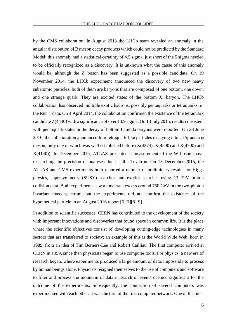
by the CMS collaboration. In August 2013 the LHCb team revealed an anomaly in the
angular distribution of B meson decay products which could not be predicted by the Standard
Model; this anomaly had a statistical certainty of 4.5 sigma, just short of the 5 sigma needed
to be officially recognized as a discovery. It is unknown what the cause of this anomaly
would be, although the Z' boson has been suggested as a possible candidate. On 19
November 2014, the LHCb experiment announced the discovery of two new heavy
subatomic particles: both of them are baryons that are composed of one bottom, one down,
and one strange quark. They are excited states of the bottom Xi baryon. The LHCb
collaboration has observed multiple exotic hadrons, possibly pentaquarks or tetraquarks, in
the Run 1 data. On 4 April 2014, the collaboration confirmed the existence of the tetraquark
candidate Z(4430) with a significance of over 13.9 sigma. On 13 July 2015, results consistent
with pentaquark states in the decay of bottom Lambda baryons were reported. On 28 June
2016, the collaboration announced four tetraquark-like particles decaying into a J/ψ and a φ
meson, only one of which was well established before (X(4274), X(4500) and X(4700) and
X(4140)). In December 2016, ATLAS presented a measurement of the W boson mass,
researching the precision of analyses done at the Tevatron. On 15 December 2015, the
ATLAS and CMS experiments both reported a number of preliminary results for Higgs
physics, supersymmetry (SUSY) searches and exotics searches using 13 TeV proton
collision data. Both experiments saw a moderate excess around 750 GeV in the two-photon
invariant mass spectrum, but the experiments did not confirm the existence of the
hypothetical particle in an August 2016 report [6][7][8][9].
In addition to scientific successes, CERN has contributed to the development of the society
with important innovations and discoveries that found space in common life. It is the place
where the scientific objectives consist of developing cutting-edge technologies in many
sectors that are transferred to society: an example of this is the World Wide Web, born in
1989, from an idea of Tim Berners-Lee and Robert Cailliau. The first computer arrived at
CERN in 1959, since then physicists began to use computer tools. For physics, a new era of
research began, where experiments produced a large amount of data, impossible to process
by human beings alone. Physicists resigned themselves to the use of computers and software
to filter and process the mountain of data in search of events deemed significant for the
outcome of the experiments. Subsequently, the connection of several computers was
experimented with each other: it was the turn of the first computer network. One of the most

THE LHC – LARGE HADRON COLLIDER
7
powerful computing centers was born at CERN, dedicated to the increasingly demanding
requirements of new experiments and the ever-increasing capacity for data acquisition of the
instruments connected to the new accelerators. Another important use of particle accelerator
is the hadronic therapy based on targeting tumors with ionizing particles. These particles
damage the DNA of the tissue cells, causing them to die. Because of their reduced ability to
repair damaged DNA, the cancer cells are particularly vulnerable to these attacks. The dose
(expressed in MeV) given by the protons to the tissue is maximum in an area of a few
millimeters, unlike electrons or X-rays. The electron beams, X-rays of different energy and
protons penetrate human tissue differently. The path taken by electrons is very short and are
useful only in areas close to the skin. X-rays penetrate more deeply but the dose absorbed
by the tissue has a typical exponential decay with increasing thickness. For protons and
heavier ions, however, the dose increases with increasing thickness up to the peak of Bragg,
which occurs just before the end of the journey. Once this peak is exceeded, the dose drops
to zero (in the case of protons) or almost to zero (in the case of heavy ions). The advantage
in the use of the latter is in the lower energy deposit in the healthy tissue surrounding the
targeted one, saving it from unnecessary damage.
8
Chapter 2
THE CMS – COMPACT MUON SOLENOID
2.1 General layout of the Experiment
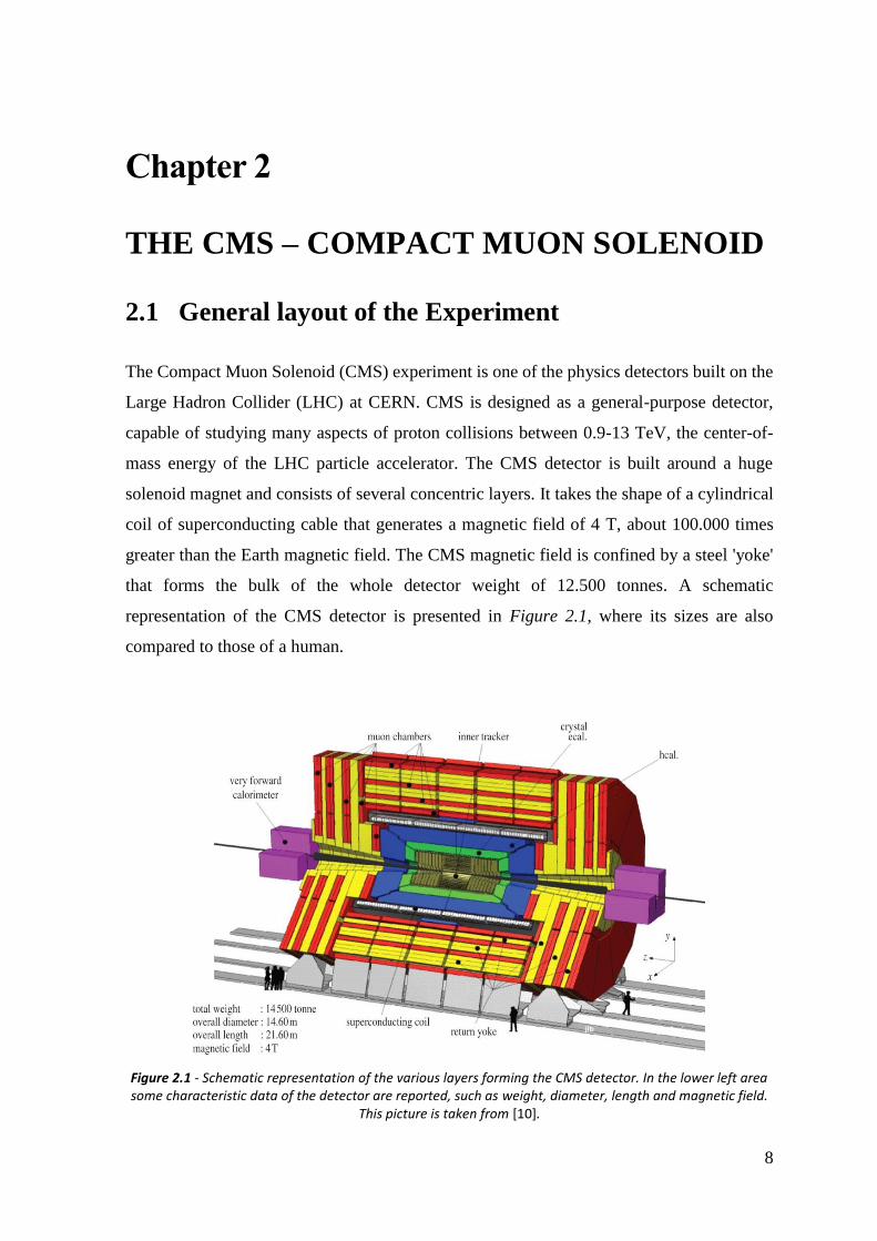
The Compact Muon Solenoid (CMS) experiment is one of the physics detectors built on the
Large Hadron Collider (LHC) at CERN. CMS is designed as a general-purpose detector,
capable of studying many aspects of proton collisions between 0.9-13 TeV, the center-of-
mass energy of the LHC particle accelerator. The CMS detector is built around a huge
solenoid magnet and consists of several concentric layers. It takes the shape of a cylindrical
coil of superconducting cable that generates a magnetic field of 4 T, about 100.000 times
greater than the Earth magnetic field. The CMS magnetic field is confined by a steel 'yoke'
that forms the bulk of the whole detector weight of 12.500 tonnes. A schematic
representation of the CMS detector is presented in Figure 2.1, where its sizes are also
compared to those of a human.
Figure 2.1 - Schematic representation of the various layers forming the CMS detector. In the lower left area some characteristic data of the detector are reported, such as weight, diameter, length and magnetic field.
This picture is taken from [10].

THE CMS – COMPACT MUON SOLENOID
9
An unusual feature of the CMS detector is that (instead of being built in-situ underground,
like the other giant detectors of the LHC experiments) it was constructed on the surface,
before being lowered underground in 15 sections and reassembled. It contains subsystems
designed to measure the energy and momentum of photons, electrons, muons, and other
products of the collisions. The innermost layer is a silicon-based tracker. The surrounding is
occupied by a scintillating crystal electromagnetic calorimeter, which is in turn surrounded
by a sampling calorimeter for hadrons. The tracker and the calorimetry are compact enough
to fit inside the CMS Solenoid which generates a powerful magnetic field of 3.8 Tesla.
Beyond the magnet, externally, there is a large muon detector, that has inside iron plates
which allow the return for the magnetic field lines. It is interesting to note that this detector
is heavier than the Eiffel Tower and it has a higher iron content than it.
2.2 The CMS Phase-2 Upgrade
An upgrade program is planned for the LHC which will smoothly bring the luminosity up to
or above 5x1034 cm-2s-1, to possibly reach an integrated luminosity of 3000 fb-1 (inverse
femtobarns). In particle physics the luminosity indicates the number of events per cross
section per unit time. This upgrade will start after 2020. In this scenario, called Phase-2,
when LHC will reach the High Luminosity phase (HL-LHC), CMS has to upgrade too, and
it will need a completely new Tracker detector, in order to fully exploit the highly-
demanding operating conditions and the delivered luminosity. The present Tracker was
designed to operate with high efficiency at an instantaneous luminosity of 1.0x1034 cm-2s-1,
with an average pileup of 20-30 collisions per bunch crossing, and up to an integrated
luminosity of 500 fb-1. The new Tracker should have also Trigger capabilities. To achieve
such goals, research and development activities are ongoing to explore options and develop
solutions. The original pixel detector has already been replaced with a new device, the Phase-
1 pixel detector, during the extended year-end technical stop of 2016/2017. The Phase-2
Tracker will have more radiation tolerance to be fully efficient up to the target integrated
luminosity, and more granularity, in order to ensure efficient tracking performance with a
high level of pileup. Other goals will be reducing material in the tracking volume, contribute
THE CMS – COMPACT MUON SOLENOID
10
to the L1 trigger and extend tracking acceptance. In section 2.4, the Tracker is presented as
it is designed for the Phase-2 Upgrade.
2.3 The Interaction Point
The interaction point represents the accelerator region where proton-proton collisions occur
between the two beams circulating in the LHC. At the collision point each beam has a radius
of 17 μm and the crossing angle between the beams is 285 μrad. At full design luminosity
each of the two LHC beams will contain 2.808 bunches of 1.15×10¹¹ protons. The interval
between crossings is 25 ns, although the number of collisions per second is only 31.6 million
due to gaps in the beam as injector magnets are activated and deactivated. To record and
save every single event, a memory with a huge capacity would be necessary. At full
luminosity each collision will produce an average of 20 proton-proton interactions. The
collisions occur at a centre of mass energy of 14 TeV. Neverless, it is worth noting that for
studies of physics at the electroweak scale, the scattering events are initiated by a single
quark or gluon from each proton, and so the actual energy involved in each collision is lower
as the total centre of mass energy is shared by these quarks and gluons.
2.4 The Tracker
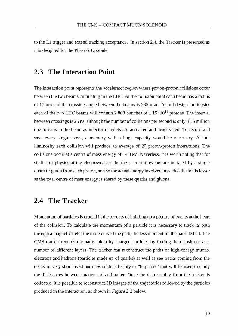
Momentum of particles is crucial in the process of building up a picture of events at the heart
of the collision. To calculate the momentum of a particle it is necessary to track its path
through a magnetic field; the more curved the path, the less momentum the particle had. The
CMS tracker records the paths taken by charged particles by finding their positions at a
number of different layers. The tracker can reconstruct the paths of high-energy muons,
electrons and hadrons (particles made up of quarks) as well as see tracks coming from the
decay of very short-lived particles such as beauty or “b quarks” that will be used to study
the differences between matter and antimatter. Once the data coming from the tracker is
collected, it is possible to reconstruct 3D images of the trajectories followed by the particles
produced in the interaction, as shown in Figure 2.2 below.
THE CMS – COMPACT MUON SOLENOID
11
Figure 2.2 - This image represents the photograph of a collision event taken by the CMS detector. The yellow curved lines represent the set of particle trajectories from the collision point to the outside. These
trajectories are reconstructed by the Tracker, and they present a helicoidal pattern as the particles are diverted in their motion by the Lorentz force produced by the magnetic field. The image has been obtained
from [11].
The tracker needs to reconstruct the tracks of charged particles with very high accuracy and
has to be as thin as possible in order to minimise the multiple scattering in the material. This
is implemented by taking position measurements so accurate that tracks can be reliably
reconstructed using just a few measurement points. Each measurement has an accuracy
around 10 µm, a fraction of the width of a human hair. As the tracker represents the
innermost layer of the detector it receives the highest volume of particles: the construction
materials were therefore carefully chosen to resist radiation. The CMS tracker is made
entirely of silicon: the pixels, at the very core of the detector and dealing with the highest
intensity of particles, and the silicon microstrip detectors that surround it. As particles travel
through the tracker the pixels and microstrips produce tiny electric signals that are amplified
and detected. The tracker is equipped with sensors covering an area that has the same size
of a tennis court, with 75 million separate electronic read-out channels. The tracker is in turn
divided into two parts: Inner Tracker and Outer Tracker.
THE CMS – COMPACT MUON SOLENOID
12
2.4.1 The Inner Tracker
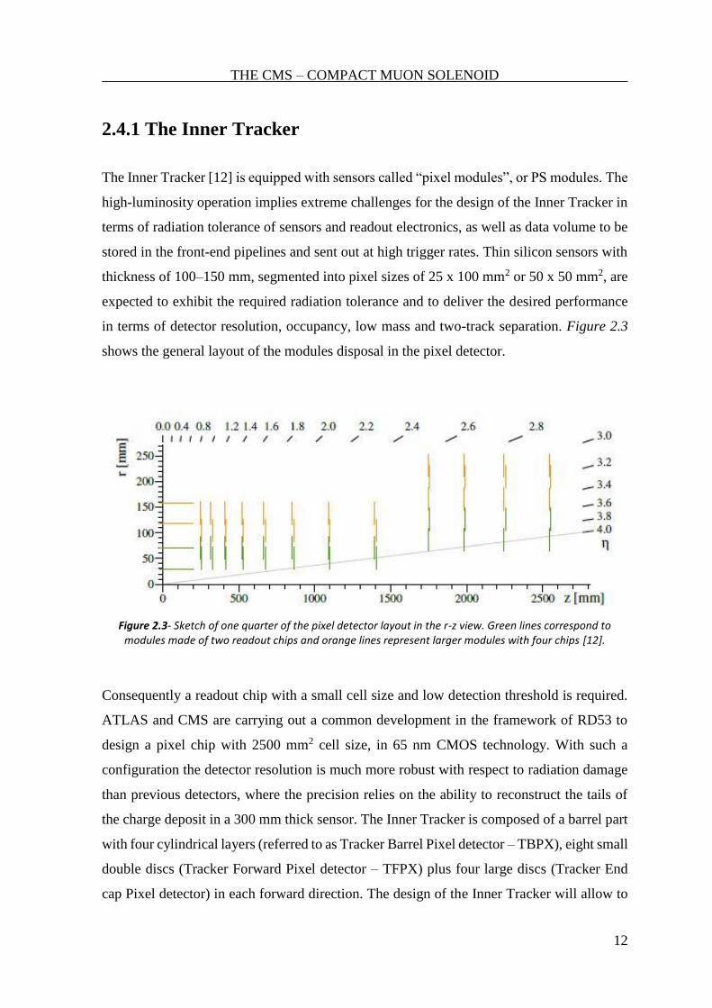
The Inner Tracker [12] is equipped with sensors called “pixel modules”, or PS modules. The
high-luminosity operation implies extreme challenges for the design of the Inner Tracker in
terms of radiation tolerance of sensors and readout electronics, as well as data volume to be
stored in the front-end pipelines and sent out at high trigger rates. Thin silicon sensors with
thickness of 100–150 mm, segmented into pixel sizes of 25 x 100 mm2 or 50 x 50 mm2, are
expected to exhibit the required radiation tolerance and to deliver the desired performance
in terms of detector resolution, occupancy, low mass and two-track separation. Figure 2.3
shows the general layout of the modules disposal in the pixel detector.
Figure 2.3- Sketch of one quarter of the pixel detector layout in the r-z view. Green lines correspond to modules made of two readout chips and orange lines represent larger modules with four chips [12].
Consequently a readout chip with a small cell size and low detection threshold is required.
ATLAS and CMS are carrying out a common development in the framework of RD53 to
design a pixel chip with 2500 mm2 cell size, in 65 nm CMOS technology. With such a
configuration the detector resolution is much more robust with respect to radiation damage
than previous detectors, where the precision relies on the ability to reconstruct the tails of
the charge deposit in a 300 mm thick sensor. The Inner Tracker is composed of a barrel part
with four cylindrical layers (referred to as Tracker Barrel Pixel detector – TBPX), eight small
double discs (Tracker Forward Pixel detector – TFPX) plus four large discs (Tracker End
cap Pixel detector) in each forward direction. The design of the Inner Tracker will allow to
THE CMS – COMPACT MUON SOLENOID
13
replace degraded parts over an extended year-end technical stop, which requires the
possibility to extract and insert the detector without removing the CMS beam pipe. This is
achieved by inserting the detector on inclined rails, necessitating a step in the radial boundary
between the Outer Tracker and the Inner Tracker. The last three double-discs of the Outer
Tracker endcap have three rings less than the first two double-discs. The Phase-2 Inner
Tracker uses all the available volume up to the mechanical structures (bulkheads) enclosing
the tracker, except for a small space close to the bulkheads that is reserved for a beam
condition monitoring device. The measurement of the luminosity will be integrated as
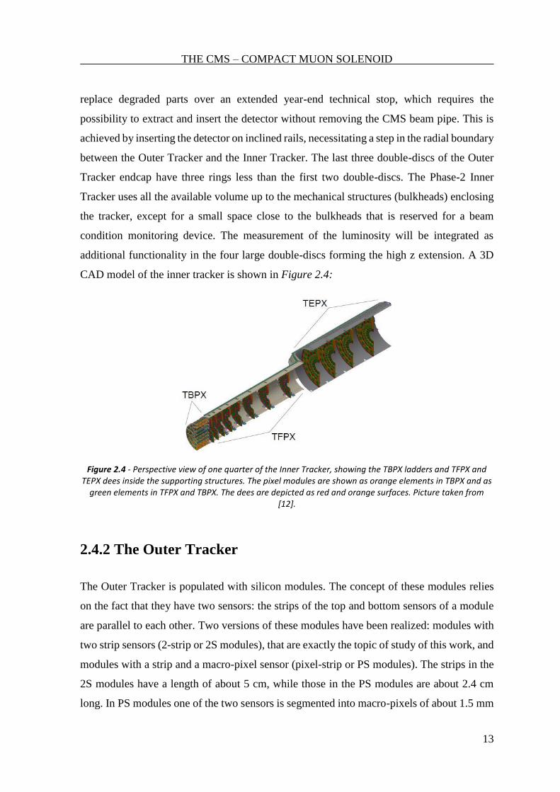
additional functionality in the four large double-discs forming the high z extension. A 3D
CAD model of the inner tracker is shown in Figure 2.4:
Figure 2.4 - Perspective view of one quarter of the Inner Tracker, showing the TBPX ladders and TFPX and TEPX dees inside the supporting structures. The pixel modules are shown as orange elements in TBPX and as
green elements in TFPX and TBPX. The dees are depicted as red and orange surfaces. Picture taken from [12].
2.4.2 The Outer Tracker
The Outer Tracker is populated with silicon modules. The concept of these modules relies
on the fact that they have two sensors: the strips of the top and bottom sensors of a module
are parallel to each other. Two versions of these modules have been realized: modules with
two strip sensors (2-strip or 2S modules), that are exactly the topic of study of this work, and
modules with a strip and a macro-pixel sensor (pixel-strip or PS modules). The strips in the
2S modules have a length of about 5 cm, while those in the PS modules are about 2.4 cm
long. In PS modules one of the two sensors is segmented into macro-pixels of about 1.5 mm
THE CMS – COMPACT MUON SOLENOID
14
length, providing the z(r) coordinate measurement in the barrel (endcaps), where z is the
axial coordinate and r is the radial coordinate of the cylinder. The PS modules are deployed
in the first three layers of the Outer Tracker, in the radial region of 200–600 mm, i.e. down
to radii at which the stub resolution remains acceptable and the data reduction effective. The
2S modules are deployed in the outermost three layers, in the radial region above 600 mm.
In the endcaps the modules are arranged in rings on disc-like structures, with the rings at low
radii, up to about 700 mm, equipped with PS modules, while 2S modules are used at larger
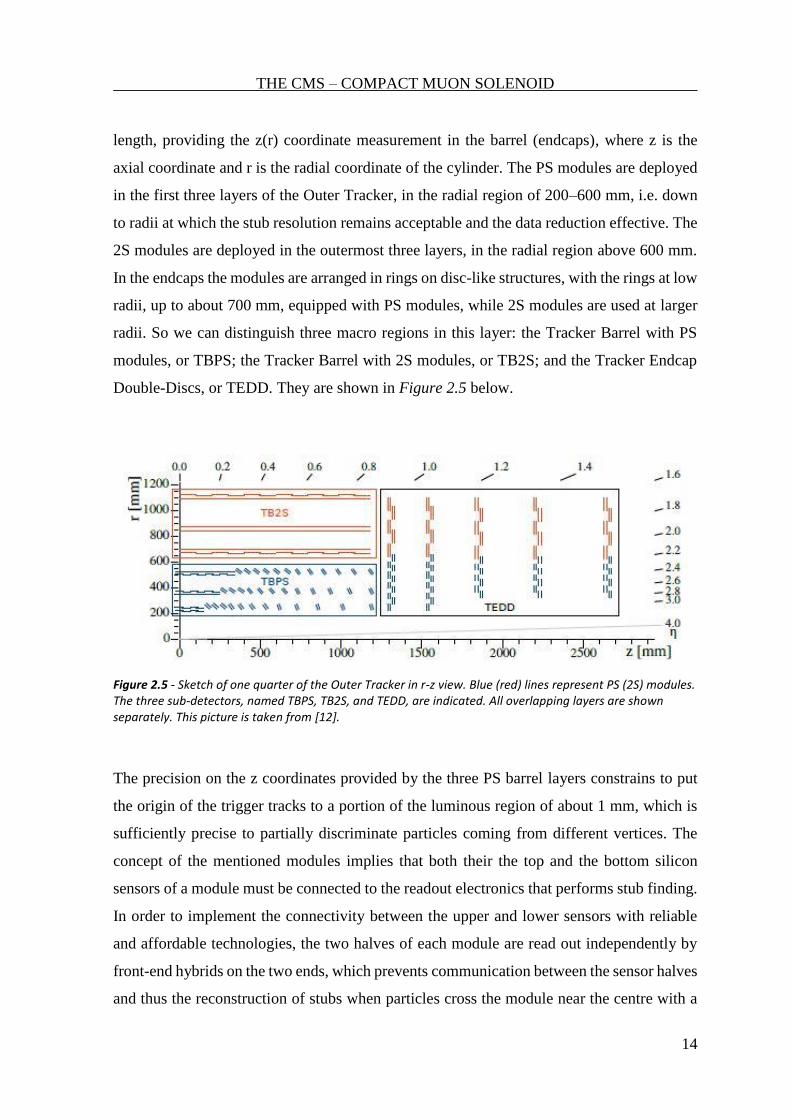
radii. So we can distinguish three macro regions in this layer: the Tracker Barrel with PS
modules, or TBPS; the Tracker Barrel with 2S modules, or TB2S; and the Tracker Endcap
Double-Discs, or TEDD. They are shown in Figure 2.5 below.
Figure 2.5 - Sketch of one quarter of the Outer Tracker in r-z view. Blue (red) lines represent PS (2S) modules. The three sub-detectors, named TBPS, TB2S, and TEDD, are indicated. All overlapping layers are shown separately. This picture is taken from [12].
The precision on the z coordinates provided by the three PS barrel layers constrains to put
the origin of the trigger tracks to a portion of the luminous region of about 1 mm, which is
sufficiently precise to partially discriminate particles coming from different vertices. The
concept of the mentioned modules implies that both their the top and the bottom silicon
sensors of a module must be connected to the readout electronics that performs stub finding.
In order to implement the connectivity between the upper and lower sensors with reliable
and affordable technologies, the two halves of each module are read out independently by
front-end hybrids on the two ends, which prevents communication between the sensor halves
and thus the reconstruction of stubs when particles cross the module near the centre with a
THE CMS – COMPACT MUON SOLENOID
15
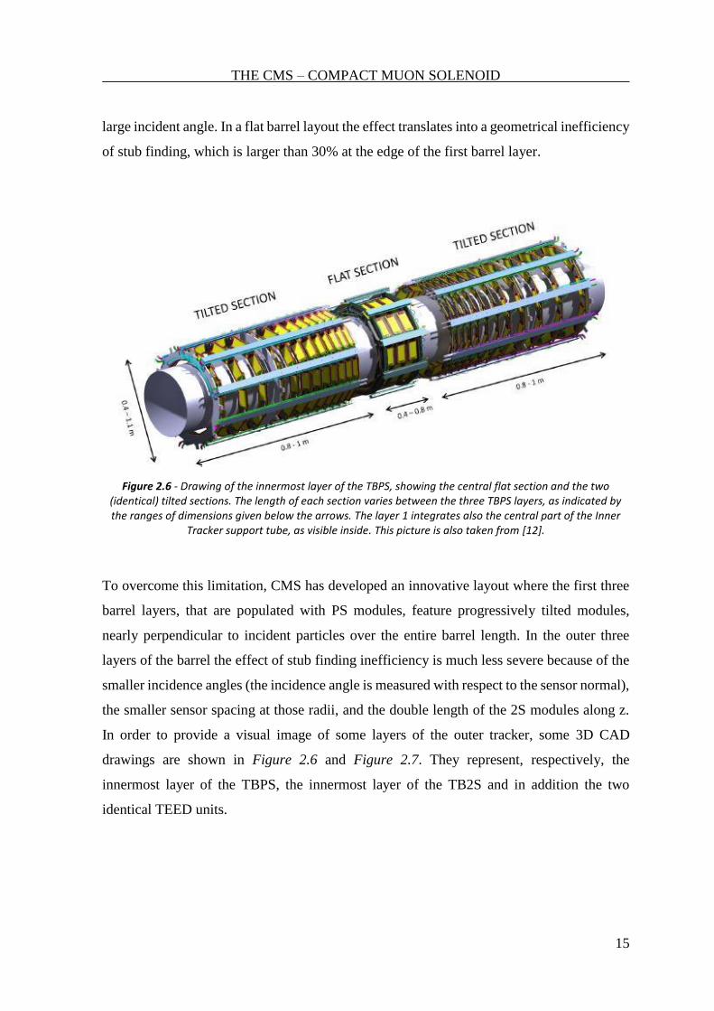
large incident angle. In a flat barrel layout the effect translates into a geometrical inefficiency
of stub finding, which is larger than 30% at the edge of the first barrel layer.
Figure 2.6 - Drawing of the innermost layer of the TBPS, showing the central flat section and the two (identical) tilted sections. The length of each section varies between the three TBPS layers, as indicated by the ranges of dimensions given below the arrows. The layer 1 integrates also the central part of the Inner
Tracker support tube, as visible inside. This picture is also taken from [12].
To overcome this limitation, CMS has developed an innovative layout where the first three
barrel layers, that are populated with PS modules, feature progressively tilted modules,
nearly perpendicular to incident particles over the entire barrel length. In the outer three
layers of the barrel the effect of stub finding inefficiency is much less severe because of the
smaller incidence angles (the incidence angle is measured with respect to the sensor normal),
the smaller sensor spacing at those radii, and the double length of the 2S modules along z.
In order to provide a visual image of some layers of the outer tracker, some 3D CAD
drawings are shown in Figure 2.6 and Figure 2.7. They represent, respectively, the
innermost layer of the TBPS, the innermost layer of the TB2S and in addition the two
identical TEED units.

THE CMS – COMPACT MUON SOLENOID
16
Figure 2.7 – On the left there is the ladders structure of the innermost layer of TB2S as installed in the support wheel. On the right there are the two identical TEDD units, each consisting of five double-discs. Each
double disc consists of four dees.
2.5 The Electromagnetic Calorimeter
The Electromagnetic Calorimeter (ECAL) [5] is placed around the vertex detector and the
Silicon Strip Tracker (described in more detail in the next section). Its aim is to measure the
energy of electromagnetically interacting particles like electrons and photons by stopping
them in an absorber of dense matter. The emerging electromagnetic shower creates photons
which are amplified and detected by silicon Avalanche Photo Diodes (APDs) and Vacuum
Phototriodes (VPTs). Lead tungstate (PbWO4) has been chosen as dense absorbing and
scintillating material [6]. It is arranged in brick-shaped crystals with a size of 23 x 2.2 x 2.2
cm3. It has excellent properties for calorimeters like a short radiation length of 0.89 cm and
a small Moliere radius of 2.2 cm; it is also radiation hard over the levels expected within 10
years of full LHC collision rate. The electromagnetic calorimeter plays an important role for
the Higgs decay mode H → γγ by detecting two photons. It is also essential for the
measurement of electrons with large transverse momenta, since these particles are clear
signatures for many interesting decays.
2.6 The Hadronic Calorimeter
The Hadronic Calorimeter (HCAL) surrounds the ECAL. It consists of an inner barrel
region, located inside the superconducting solenoid, an outer barrel part inside the iron return

THE CMS – COMPACT MUON SOLENOID
17
yoke of the magnet, two end caps and two very forward calorimeters. The latter ones are
called Hadron Forward (HF) calorimeters and they are placed outside the magnet return yoke
at about 12 m from the interaction point. In contrast to the homogeneous ECAL, the HCAL
is a sampling type calorimeter made of copper as absorber material and mostly plastic
scintillators in between as light emitting active material. Devices to shift wavelength are
used to guide the signals from the scintillators to the endcap region, where APDs and
Proximity Focused Hybrid Photo Diodes (PFHPD) are converting and amplifying them to
electrical signals. In the HF, quartz fibres embedded into copper absorbers are used as
scintillators. Hadrons strongly interact with nuclei in the copper absorbers creating hadronic
jets. The energy of these jets is determined, as well as missing transverse energy which is
possible to reconstruct the hermetic design of the HCAL.
2.7 The Superconducting Solenoid
The superconducting magnet surrounds the tracking detectors, the ECAL and most parts of
the HCAL. It plays an essential role for the momentum measurement of charged particles by
deflecting their track while they are produced at the interaction point. Most parts of the
calorimeters are also placed inside the solenoid to reduce the absorbing material in front of
them, which increases their energy resolution. The magnet coil has a length of about 12.5 m,
a diameter of about 6 m and it is made of superconducting Niobium Titanium (NiTi) wires,
powered by an electrical current of 20,000 Amperes to reach the nominal magnetic field of
4 Tesla. The solenoidal shape of the field lines is closed by an iron return yoke surrounding
the coil, in which the muon detectors are installed.
2.8 The Muon System
The outermost detectors are embedded into the iron return yoke of the superconducting
magnet. This contributes to make this layer much more radial in relations to the others. The
muon System occupies a considerable volume percentage in the detector, as it is shown in
Figure 2.8, where it is possible to find, through a sectional view, the general summary layout
of the previous layers. Three different gaseous detector systems are used for the detection of
THE CMS – COMPACT MUON SOLENOID
18
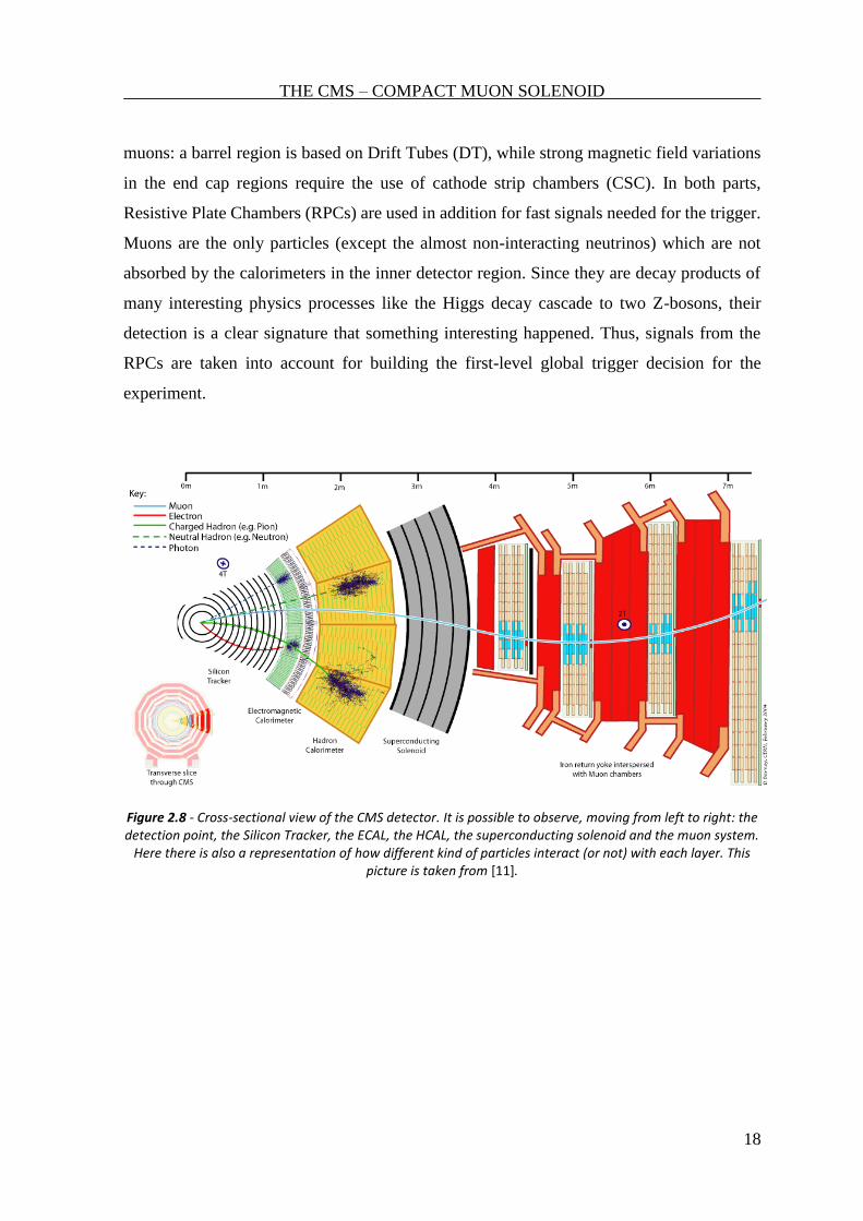
muons: a barrel region is based on Drift Tubes (DT), while strong magnetic field variations
in the end cap regions require the use of cathode strip chambers (CSC). In both parts,
Resistive Plate Chambers (RPCs) are used in addition for fast signals needed for the trigger.
Muons are the only particles (except the almost non-interacting neutrinos) which are not
absorbed by the calorimeters in the inner detector region. Since they are decay products of
many interesting physics processes like the Higgs decay cascade to two Z-bosons, their
detection is a clear signature that something interesting happened. Thus, signals from the
RPCs are taken into account for building the first-level global trigger decision for the
experiment.
Figure 2.8 - Cross-sectional view of the CMS detector. It is possible to observe, moving from left to right: the detection point, the Silicon Tracker, the ECAL, the HCAL, the superconducting solenoid and the muon system.
Here there is also a representation of how different kind of particles interact (or not) with each layer. This picture is taken from [11].
19
Chapter 3
THE 2S - 2 STRIPS MODULE OF THE
OUTER SILICON TRACKER IN CMS
3.1 Operating Fundamentals of Silicon Sensors
Semiconductor sensors are electronic devices widely used in the field of high-energy
experimental physics in order to detect the passage of a particle and to measure its energy.
The operating principle is based on the collection of charges inside a depleted region of a p-
n junction due to the ionization caused by the passage of particles through the semiconductor.
A peculiarity of these devices is that they are particularly suitable for carrying out precision
measurements relating to the determination of the average life of short-lived subnuclear
particles and the trajectory they travel; this is made possible by the high spatial resolution of
these sensors. Another advantage is their compactness, their ability to work well at low
temperatures and in presence of strong magnetic fields, a feature that makes their use
desirable inside the particle detectors placed along the LHC. Moreover, only 3.66 eV are
needed to generate an electron-hole pair, by comparison with the 30 eV of a gas detector. It
should also be remembered that they exhibit good resistance to damage and degradation of
performance when subjected to massive doses of radiation. The CMS detector is equipped
with single-sided semiconductor p+ n- sensors that allow the application of high substrate
bias voltages. This is necessitated due to the inversion effect of the substrate type due to high
radiation doses; therefore, to ensure that the device works properly over time, it must be
over-saturated. Moreover, since the sensors have to maintain their functionality over time, it
is also necessary that they work at an operating temperature of -10° C or less. Single-sided
sensors are less sensitive to radiation damage than double-sided detectors; they are also much
cheaper. From the back-to-back approach of two single-sided detectors, rotated 90° with
respect to each other, it is possible to reconstruct two coordinates. The sensor is made on a
wafer of material n with a thickness of 300 microns. On one face of this structure (n-side) a
n+ layer is made, while on the other (p-side) microstructures p+ implants are present. Above
these microstructures, separated by a thin insulator, polysilicon tracks are deposited and
THE 2S – 2 STRIPS MODULE OF THE OUTER SILICON TRACKER IN CMS
20
subsequently metallized. The distance between a microstrip and the other ("pitch") is one of
the factors determining the spatial resolution, which obviously improves as spacing
decreases. However, this distance cannot be excessively reduced, otherwise there may be
unwanted phenomena of capacitive coupling between the adjacent microstrips. An electric
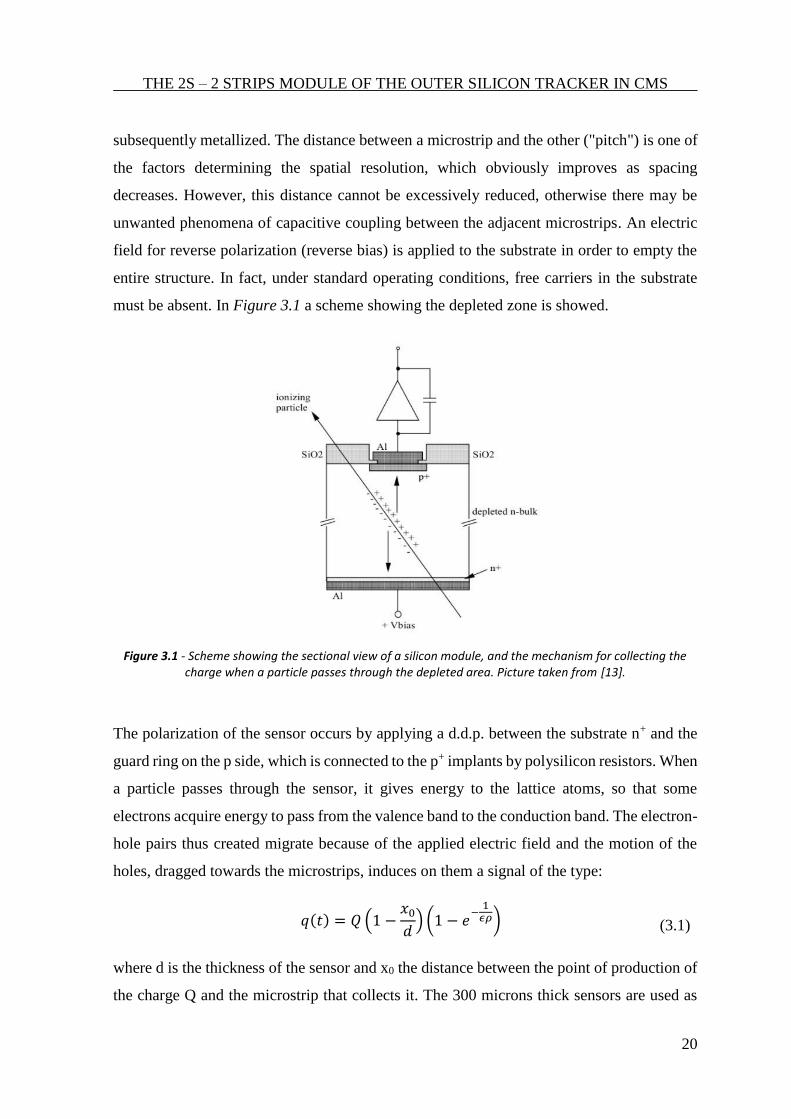
field for reverse polarization (reverse bias) is applied to the substrate in order to empty the
entire structure. In fact, under standard operating conditions, free carriers in the substrate
must be absent. In Figure 3.1 a scheme showing the depleted zone is showed.
Figure 3.1 - Scheme showing the sectional view of a silicon module, and the mechanism for collecting the charge when a particle passes through the depleted area. Picture taken from [13].
The polarization of the sensor occurs by applying a d.d.p. between the substrate n+ and the
guard ring on the p side, which is connected to the p+ implants by polysilicon resistors. When
a particle passes through the sensor, it gives energy to the lattice atoms, so that some
electrons acquire energy to pass from the valence band to the conduction band. The electron-
hole pairs thus created migrate because of the applied electric field and the motion of the
holes, dragged towards the microstrips, induces on them a signal of the type:
𝑞(𝑡) = 𝑄 (1 −
𝑥0
𝑑) (1 − 𝑒
−1
𝜖𝜌) (3.1)
where d is the thickness of the sensor and x0 the distance between the point of production of
the charge Q and the microstrip that collects it. The 300 microns thick sensors are used as
THE 2S – 2 STRIPS MODULE OF THE OUTER SILICON TRACKER IN CMS
21
vertex detectors, i.e. they operate the reconstruction of the trajectory of the particles. They
have an efficient spatial resolution, since in this way the charge is collected by a limited
number of microstrips, allowing to determine with good precision the point of passage of
the particle. However, due to the reduced thickness of the substrate, all particles give the
same energy to the material and therefore the same amount of charge is generated by
ionization. While this is unimportant to determine the passage point, this does not allow to
distinguish the type of particle that has passed through the sensor. The information collected
from these sensors must be available for reading and interpretation by a front-end reading
architecture. From an electrical point of view, the single microstrip is seen at the input of the
reading electronics as a capacitive network.
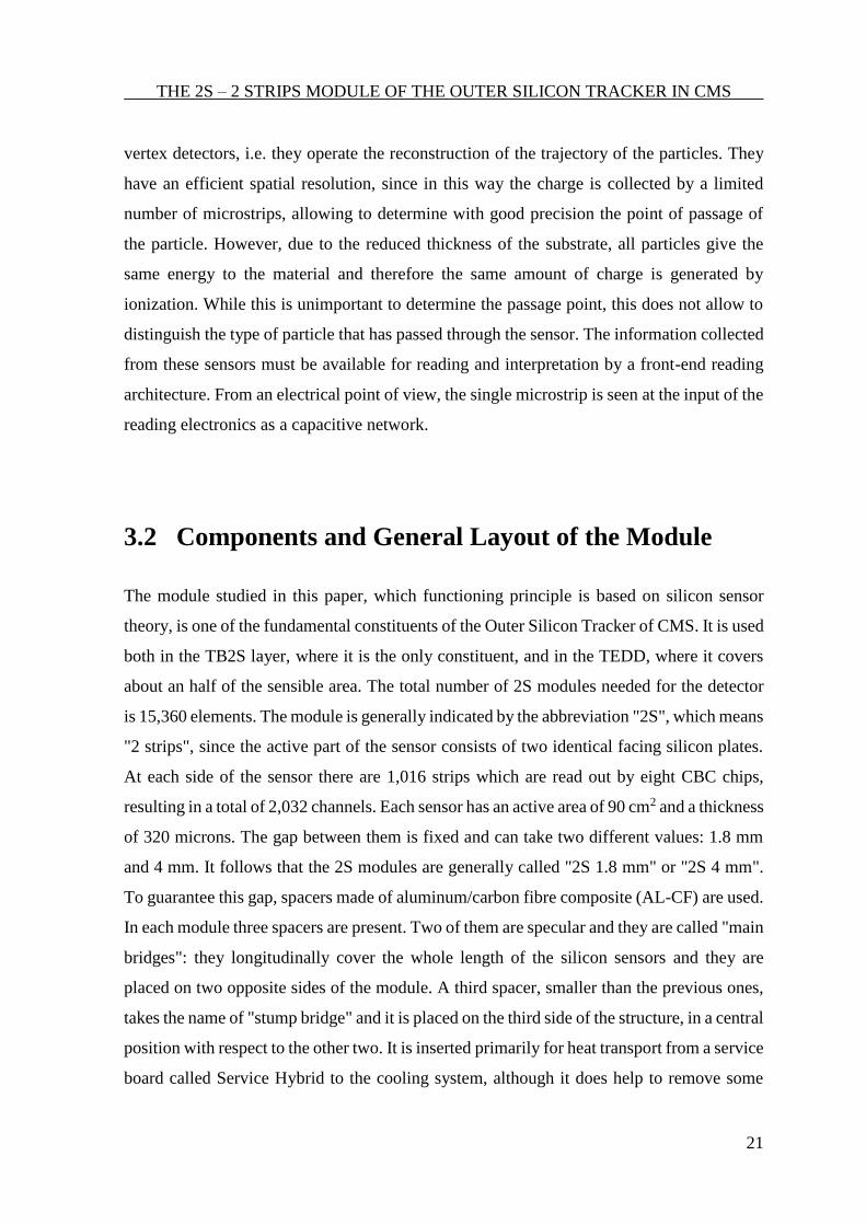
3.2 Components and General Layout of the Module
The module studied in this paper, which functioning principle is based on silicon sensor
theory, is one of the fundamental constituents of the Outer Silicon Tracker of CMS. It is used
both in the TB2S layer, where it is the only constituent, and in the TEDD, where it covers
about an half of the sensible area. The total number of 2S modules needed for the detector
is 15,360 elements. The module is generally indicated by the abbreviation "2S", which means
"2 strips", since the active part of the sensor consists of two identical facing silicon plates.
At each side of the sensor there are 1,016 strips which are read out by eight CBC chips,
resulting in a total of 2,032 channels. Each sensor has an active area of 90 cm2 and a thickness
of 320 microns. The gap between them is fixed and can take two different values: 1.8 mm
and 4 mm. It follows that the 2S modules are generally called "2S 1.8 mm" or "2S 4 mm".
To guarantee this gap, spacers made of aluminum/carbon fibre composite (AL-CF) are used.
In each module three spacers are present. Two of them are specular and they are called "main
bridges": they longitudinally cover the whole length of the silicon sensors and they are
placed on two opposite sides of the module. A third spacer, smaller than the previous ones,
takes the name of "stump bridge" and it is placed on the third side of the structure, in a central
position with respect to the other two. It is inserted primarily for heat transport from a service
board called Service Hybrid to the cooling system, although it does help to remove some
THE 2S – 2 STRIPS MODULE OF THE OUTER SILICON TRACKER IN CMS
22
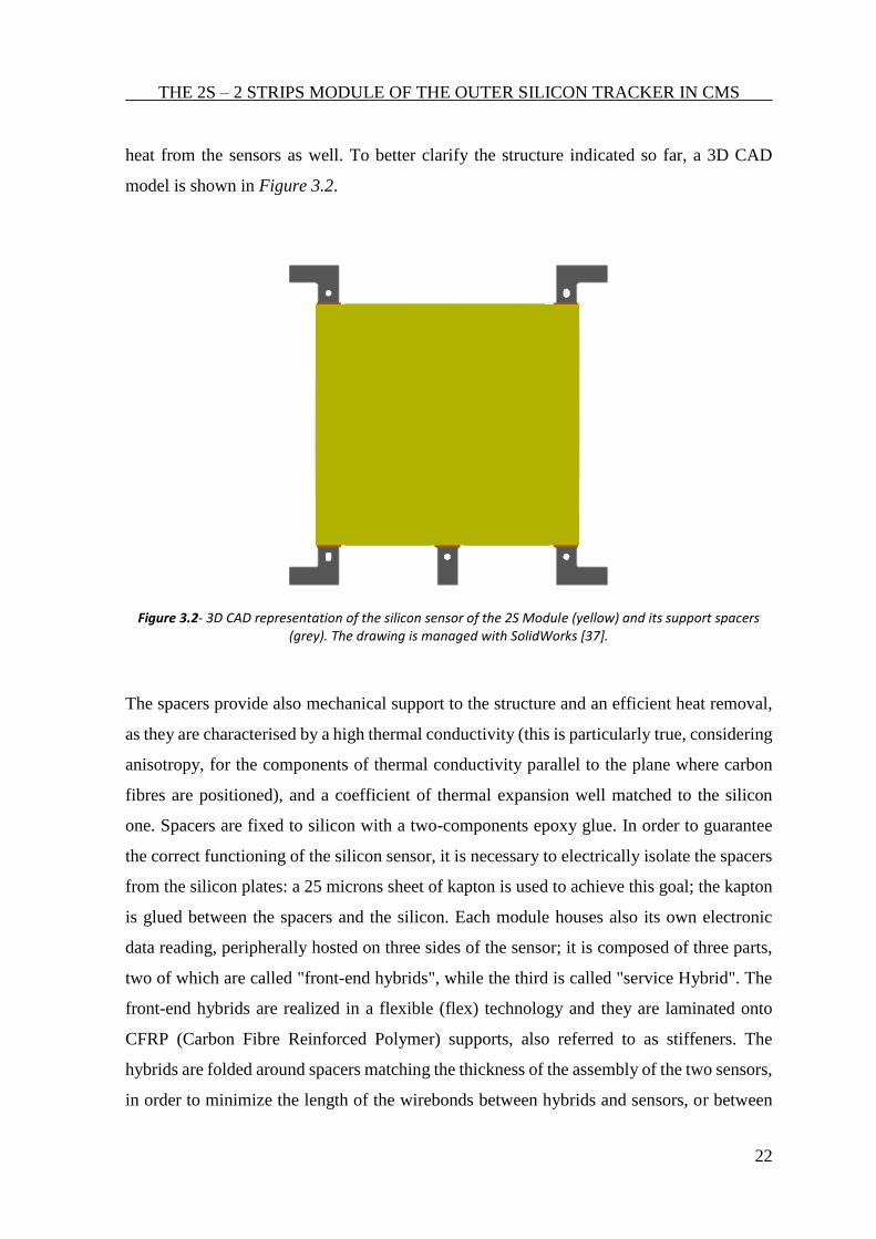
heat from the sensors as well. To better clarify the structure indicated so far, a 3D CAD
model is shown in Figure 3.2.
Figure 3.2- 3D CAD representation of the silicon sensor of the 2S Module (yellow) and its support spacers (grey). The drawing is managed with SolidWorks [37].
The spacers provide also mechanical support to the structure and an efficient heat removal,
as they are characterised by a high thermal conductivity (this is particularly true, considering
anisotropy, for the components of thermal conductivity parallel to the plane where carbon
fibres are positioned), and a coefficient of thermal expansion well matched to the silicon
one. Spacers are fixed to silicon with a two-components epoxy glue. In order to guarantee
the correct functioning of the silicon sensor, it is necessary to electrically isolate the spacers
from the silicon plates: a 25 microns sheet of kapton is used to achieve this goal; the kapton
is glued between the spacers and the silicon. Each module houses also its own electronic
data reading, peripherally hosted on three sides of the sensor; it is composed of three parts,
two of which are called "front-end hybrids", while the third is called "service Hybrid". The
front-end hybrids are realized in a flexible (flex) technology and they are laminated onto
CFRP (Carbon Fibre Reinforced Polymer) supports, also referred to as stiffeners. The
hybrids are folded around spacers matching the thickness of the assembly of the two sensors,
in order to minimize the length of the wirebonds between hybrids and sensors, or between
THE 2S – 2 STRIPS MODULE OF THE OUTER SILICON TRACKER IN CMS
23
hybrids and MPA periphery in the case of PS modules. One 2S front-end hybrid carries eight
CMS Binary Chips (CBCs) reading out the strips of the top and bottom sensors at one sensor
end, plus the Concentrator Integrated Circuit (CIC), which serves as interface between all
the CBCs of the hybrid and the readout link. The role of the CIC is mainly to aggregate and
serialize the data of the readout chips and to distribute them clock, trigger, and control
signals. One PS front-end hybrid houses eight Short Strip ASICs (SSAs) reading out the strip
sensor, and the same CIC as used for 2S hybrids. All the front-end chips implement binary
readout. At the aim of fully exploiting the achievable hit position resolution in the on-module
stub finding, which compares cluster positions, in both module types one extra bit is added
to the hit address, so that in the case of clusters with an even number of fired channels, the
coordinate is set in the centre of the cluster, in between the two channels (“half-strip
resolution”). The auxiliary electronics for powering and optical readout is integrated on
service hybrids realized in the same flex technology as the front-end hybrids. The service
hybrids are also laminated onto stiffeners. In 2S modules one single service hybrid is located
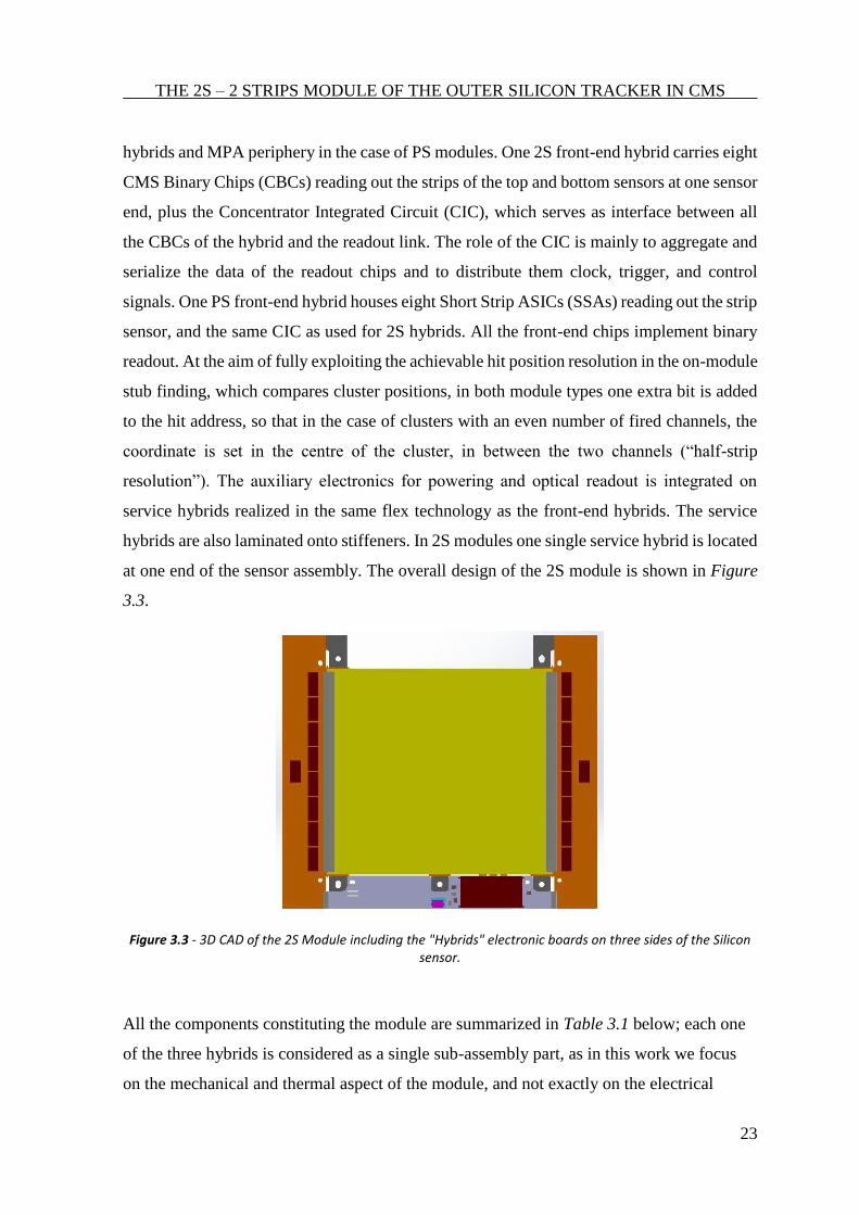
at one end of the sensor assembly. The overall design of the 2S module is shown in Figure
3.3.
Figure 3.3 - 3D CAD of the 2S Module including the "Hybrids" electronic boards on three sides of the Silicon sensor.
All the components constituting the module are summarized in Table 3.1 below; each one
of the three hybrids is considered as a single sub-assembly part, as in this work we focus
on the mechanical and thermal aspect of the module, and not exactly on the electrical

THE 2S – 2 STRIPS MODULE OF THE OUTER SILICON TRACKER IN CMS
24
behaviour. However, it has to be remembered that each of the hybrids has its characteristic
components that are in turn assembled together.
Component N° of elements
per module
Colors in Figure13
Silicon Sensor 2 Yellow
Main bridge 2 Dark Gray
Stump Bridge 1 Dark Gray
Left Hybrid 1 Orange/Red
Right Hybrid 1 Orange/Red
Service Hybrid 1 Light gray/Red
Kapton sheet 6 Light Orange
Glue Layers 12 Not Visible
Wire bonding - Encapsulation 8 Medium Gray
Table 3.1 - Types of components that make up a single 2S module and their respective quantities. The last column on the right also shows the colours with which they are represented in the CAD drawing of Figure 12.
Each module is therefore housed in a linear ladder structure (in the case of TB2S detector)
or disc shaped supports (in TEDD). The TB2S ladders are made of two parallel carbon fibre
C-shaped profiles, joined by several orthogonal elements (referred to as cross pieces), also
made of carbon fibre. The modules are supported by machined inserts, built in aluminium
carbon fibre composite material, supported by the C-shaped profiles. These inserts also
provide a connection to the cooling pipe that transits the full length of the ladder and back,
forming a U-shaped circuit. The ladder structure is shown in Figure 3.4a. On the other hand,
in TEDD, modules are mounted in discs, which for assembly reasons, are split in half-discs,
or “dees”. Two discs are grouped to form one double disc, which provides one hermetic
detector plane. In this case the cooling circuitry is made in sectors. The cooling pipes are up
to 8 m long and have many bends in order to reach every module in the sector. Carbon foam
blocks and aluminium inserts are used to provide thermal contacts between the modules and
the cooling pipes. This second type of use and positioning for the 2S module in the outer
Tracker is presented in Figure 3.4b.
THE 2S – 2 STRIPS MODULE OF THE OUTER SILICON TRACKER IN CMS
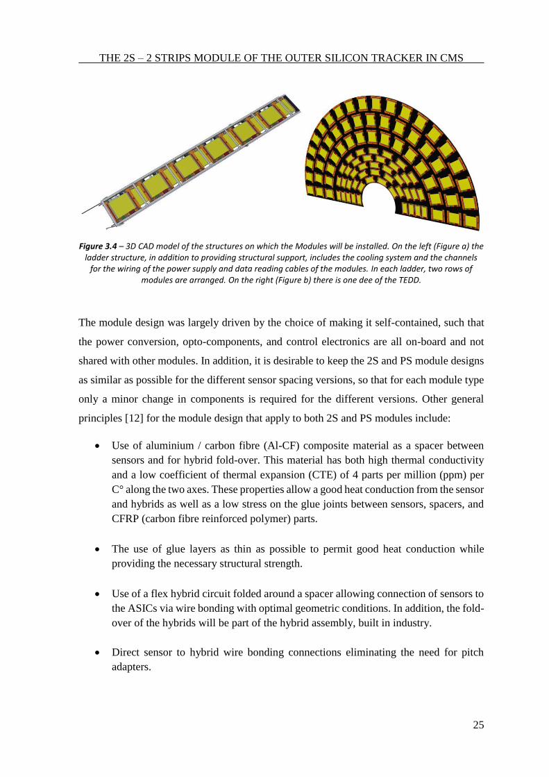
25
Figure 3.4 – 3D CAD model of the structures on which the Modules will be installed. On the left (Figure a) the ladder structure, in addition to providing structural support, includes the cooling system and the channels
for the wiring of the power supply and data reading cables of the modules. In each ladder, two rows of modules are arranged. On the right (Figure b) there is one dee of the TEDD.
The module design was largely driven by the choice of making it self-contained, such that
the power conversion, opto-components, and control electronics are all on-board and not
shared with other modules. In addition, it is desirable to keep the 2S and PS module designs
as similar as possible for the different sensor spacing versions, so that for each module type
only a minor change in components is required for the different versions. Other general
principles [12] for the module design that apply to both 2S and PS modules include:
• Use of aluminium / carbon fibre (Al-CF) composite material as a spacer between
sensors and for hybrid fold-over. This material has both high thermal conductivity
and a low coefficient of thermal expansion (CTE) of 4 parts per million (ppm) per
C° along the two axes. These properties allow a good heat conduction from the sensor
and hybrids as well as a low stress on the glue joints between sensors, spacers, and
CFRP (carbon fibre reinforced polymer) parts.
• The use of glue layers as thin as possible to permit good heat conduction while
providing the necessary structural strength.
• Use of a flex hybrid circuit folded around a spacer allowing connection of sensors to
the ASICs via wire bonding with optimal geometric conditions. In addition, the fold-
over of the hybrids will be part of the hybrid assembly, built in industry.
• Direct sensor to hybrid wire bonding connections eliminating the need for pitch
adapters.

THE 2S – 2 STRIPS MODULE OF THE OUTER SILICON TRACKER IN CMS
26
The bond pad pitch of the hybrid is identical to that of the sensor, simplifying the
wire bonding. The electrical lines are routed further to the bump bond pads on the
hybrid, where the chips are connected via bump bonding.
• Use of high reliability connectors, where possible, between service hybrids and front-
end
Hybrids, as well as for the connection to the backplane bias circuit. As a fall-back
solution, connectivity between hybrids would be realized through wire bonding.
• Encapsulation of all wire bonds to reduce risk of handling damage and damage due
to possible resonant vibrations in the magnetic field.
• The HV isolation requirement is 1,000 V between any conductive structures at high
voltage
and those at ground potential. This gives a safety margin of 400 V with respect to the
nominal bias voltage of 600 V, and still 200 V margin with respect to the maximum
sensor bias voltage of 800 V, considered to be used in order to increase the signal, if
it shall ever be required.
• Use of kapton MT polyimide films of 25 mm thickness for HV isolation between
sensors
and Al-CF spacers. It provides a reliable barrier and it has a relatively high thermal
conductivity.
• The HV bias connection to the 2S strip sensors will use a small flex circuit glued to
the back of the bare sensor before assembly. Then, it will be wire bonded to the
sensor backplane and encapsulated to protect the wires. One thermistor, read out by
the LpGBT, is also mounted on a kapton flex circuit and it will be glued to the top
sensor in each module. Both the HV bias and the thermistor circuit will have a
connector tail so they can be connected to the service hybrid (temperature sensors
and bias circuit in 2S modules) or the front-end hybrid.
3.3 Cooling and Thermal Requirements
Temperature plays a fundamental role in the functioning of semiconductor devices: it is
directly connected to the vibration of particles, and the higher it is, the higher is the
probability that the particles move from one energy band to the other. The ideal condition
for the particles not to pass spontaneously from one band to another, is to have an operating
temperature of 0 K, but this constitutes a theoretical limit for physics. However, it is
THE 2S – 2 STRIPS MODULE OF THE OUTER SILICON TRACKER IN CMS
27
nevertheless true that lower is the working temperature, the better is the functioning of
devices. Silicon sensors, being semiconductor materials, require a temperature not higher
than -20 °C for their optimal functioning. However, there are multiple sources of thermal
power in each module, which tend to increase their temperature. The first source of heat is
the silicon sensor itself, because by applying the reverse bias voltage, leakage currents
always appear. It is possible to provide an estimate of this current with the formula obtained
by [14]:
𝑃𝑠𝑒𝑛𝑠𝑜𝑟(𝑇, ∆𝐸) ≈ 𝑃0
𝑇2
𝑇02 𝑒𝑥𝑝 (−
∆𝐸
2𝑘𝐵(
1
𝑇−
1
𝑇0)) (3.3)
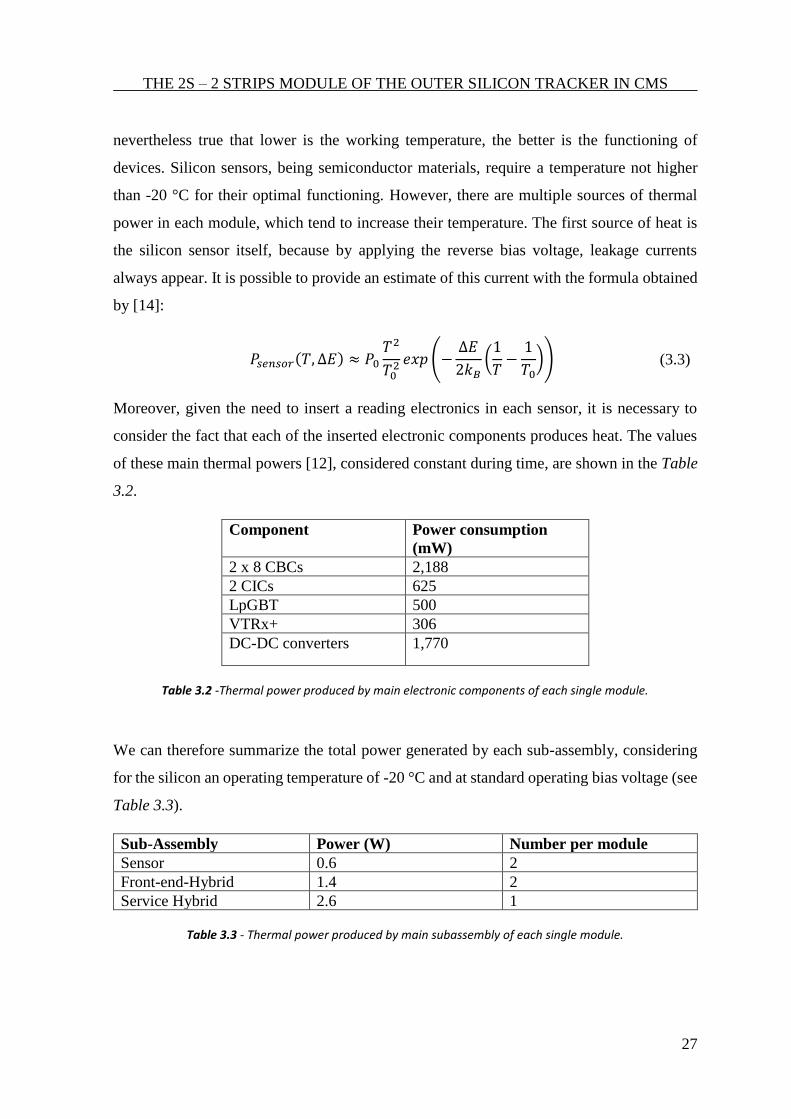
Moreover, given the need to insert a reading electronics in each sensor, it is necessary to
consider the fact that each of the inserted electronic components produces heat. The values
of these main thermal powers [12], considered constant during time, are shown in the Table
3.2.
Component Power consumption
(mW)
2 x 8 CBCs 2,188
2 CICs 625
LpGBT 500
VTRx+ 306
DC-DC converters 1,770
Table 3.2 -Thermal power produced by main electronic components of each single module.
We can therefore summarize the total power generated by each sub-assembly, considering
for the silicon an operating temperature of -20 °C and at standard operating bias voltage (see
Table 3.3).
Sub-Assembly Power (W) Number per module
Sensor 0.6 2
Front-end-Hybrid 1.4 2
Service Hybrid 2.6 1
Table 3.3 - Thermal power produced by main subassembly of each single module.
THE 2S – 2 STRIPS MODULE OF THE OUTER SILICON TRACKER IN CMS
28
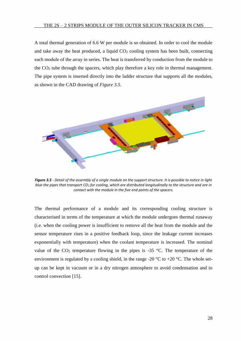
A total thermal generation of 6.6 W per module is so obtained. In order to cool the module
and take away the heat produced, a liquid CO2 cooling system has been built, connecting
each module of the array in series. The heat is transferred by conduction from the module to
the CO2 tube through the spacers, which play therefore a key role in thermal management.
The pipe system is inserted directly into the ladder structure that supports all the modules,
as shown in the CAD drawing of Figure 3.5.
Figure 3.5 - Detail of the assembly of a single module on the support structure. It is possible to notice in light blue the pipes that transport CO2 for cooling, which are distributed longitudinally to the structure and are in
contact with the module in the five end points of the spacers.
The thermal performance of a module and its corresponding cooling structure is
characterised in terms of the temperature at which the module undergoes thermal runaway
(i.e. when the cooling power is insufficient to remove all the heat from the module and the
sensor temperature rises in a positive feedback loop, since the leakage current increases
exponentially with temperature) when the coolant temperature is increased. The nominal
value of the CO2 temperature flowing in the pipes is -35 °C. The temperature of the
environment is regulated by a cooling shield, in the range -20 °C to +20 °C. The whole set-
up can be kept in vacuum or in a dry nitrogen atmosphere to avoid condensation and to
control convection [15].
THE 2S – 2 STRIPS MODULE OF THE OUTER SILICON TRACKER IN CMS
29
3.4 Module Assembly
The module construction consists basically on the assembly of the following elements: two
sensors, three spacers, and three hybrids for the 2S modules; they are realised by various
suppliers who collaborate with CMS. The construction of 2S modules is based primarily on
manual jig-based assembly techniques. Each Jig is made with machine tools and has very
tight tolerances, in order to guarantee the necessary precision. Each of its dimensions is
subjected to quality control by means of metrology machines before it is applied for
assembly. A robot-based module assembly, as was used in the existing CMS silicon strip
tracker, is not adopted for two reasons. First, the back-to-back sensor arrangement poses
numerous problems for placement, precision alignment and retaining the positioning during
glue curing. Second, even in a robotic assembly a very large amount of human intervention
is needed: unpacking, inventory, visual inspection, component selection and placement,
programming and surveillance of the robot, inspection of assembly results, handling, testing,
storing, and packing. The specifications for the sensor to sensor alignment during assembly
are: a distance perpendicular to the strips of Dx < 50 mm, a distance along the strips of Dy <
100 mm, and a tilt angle between the strips smaller than 400 mrad in 2S modules. Kapton
isolation foils are used to isolate the spacers, which are at ground potential, against the
backplane of the sensors, where the bias voltage is applied. The first step in 2S module
assembly is thus the gluing of the kapton isolation foils to the backplane of the sensors. The
three kapton foils will be stamp cut in industry with a high precision, using kapton MT sheets
of 25 mm thickness. At the same time, the HV bias circuit, produced by a qualified flex
circuit manufacturer, can be glued. This assembly step will require two assembly jigs. One
jig is used to accurately position the very small and thin kapton parts for vacuum pick-up,
used to transfer the foils to the second jig, which holds the sensor in a precise and stable
position. The glue used for the kapton to sensor joint can be distributed with a dispensing
robot in order to provide a precise volume of glue on the backplane of the sensor. The glue
to be used is a low viscosity, two parts epoxy adhesive with a long working time and suitable
for room temperature curing. It must be electronics grade since it will be in contact with the
back side of the sensors, it has not to degrade the HV isolation between the parts of the sensor
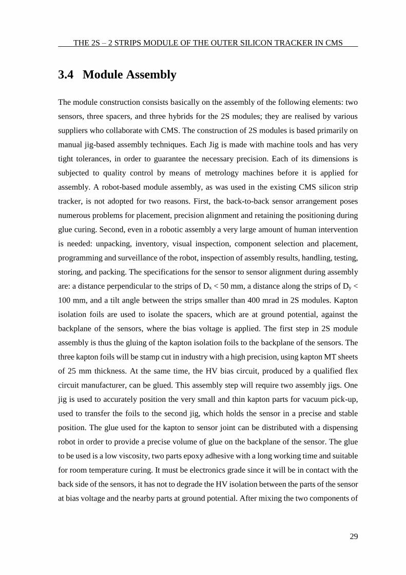
at bias voltage and the nearby parts at ground potential. After mixing the two components of
THE 2S – 2 STRIPS MODULE OF THE OUTER SILICON TRACKER IN CMS
30
the epoxy glue and before putting it on the foils, the mixture is kept in a vacuum chamber to
remove any air bubbles trapped in the glue as shown in Figure 3.6
Figure 1 -On the left side it is possible to see the two-component Polytech Ep-601 epoxy adhesive used for kapton gluing. On the right is the device with which the vacuum is obtained: it is a vessel consisting of two
shells between which a gasket is placed, which through a small tube can be connected to a centralized laboratory vacuum system.
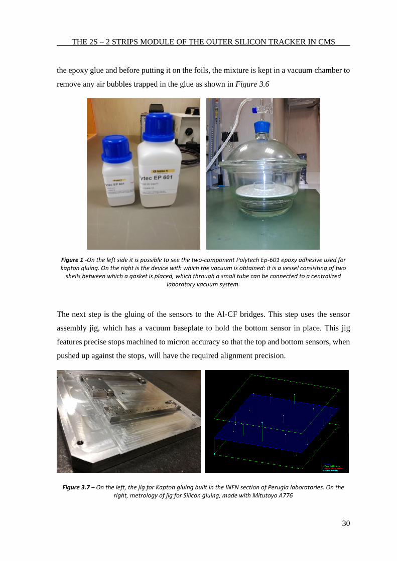
The next step is the gluing of the sensors to the Al-CF bridges. This step uses the sensor
assembly jig, which has a vacuum baseplate to hold the bottom sensor in place. This jig
features precise stops machined to micron accuracy so that the top and bottom sensors, when
pushed up against the stops, will have the required alignment precision.
Figure 3.7 – On the left, the jig for Kapton gluing built in the INFN section of Perugia laboratories. On the right, metrology of jig for Silicon gluing, made with Mitutoyo A776

THE 2S – 2 STRIPS MODULE OF THE OUTER SILICON TRACKER IN CMS
31
After gluing Kapton on sensors using a gluing Jig (Figure 3.7), the steps for sensor assembly
are following described: placement of the bottom sensor, application of vacuum, application
of glue to the two sides of the Al-CF bridges using a glue transfer jig. Glue is painted or
rolled onto the surface of the glue transfer jig, which is designed so that only the part of the
bridge needing glue receives it when the piece is guided down onto the surface using
precision pins. Then, the bridges can be lowered onto the bottom sensor, again using
precision pins. The top sensor can then be placed on the top of the bridges, pushing the sensor
against the stops to achieve alignment with the bottom sensor. Then, a weight plate is placed
on the top sensor to apply a uniform force over the gluing zones, so that the glue will be
squeezed to a thin layer. This plate has foam bars glued to the bottom so that the contact to
the sensor is compliant and will not damage the sensor active surface. The whole jig can go
into a vacuum chamber, with the purpose of removing air bubbles if formed. All the
mechanical assembly phases are followed by a strict tolerance control through metrology
measuring machines, such as the Mitutoyo A776 (see Figure 3.8), available at the INFN
laboratory in Perugia, where the module studied was assembled.
Figure 3.8 - On the left the Silicon sensor installed on a specific measuring jig. The Jig holds the sensor creating a vacuum on the interface. The Jig in turn has holes in the lower part that allow it to be placed on
the granite surface of the Mitutoyo A776 measuring machine, shown on the right.
THE 2S – 2 STRIPS MODULE OF THE OUTER SILICON TRACKER IN CMS
32
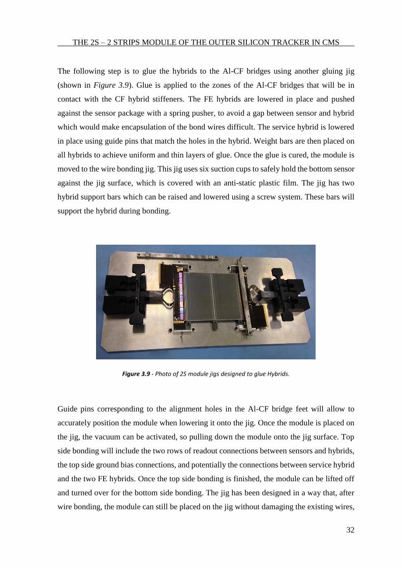
The following step is to glue the hybrids to the Al-CF bridges using another gluing jig
(shown in Figure 3.9). Glue is applied to the zones of the Al-CF bridges that will be in
contact with the CF hybrid stiffeners. The FE hybrids are lowered in place and pushed
against the sensor package with a spring pusher, to avoid a gap between sensor and hybrid
which would make encapsulation of the bond wires difficult. The service hybrid is lowered
in place using guide pins that match the holes in the hybrid. Weight bars are then placed on
all hybrids to achieve uniform and thin layers of glue. Once the glue is cured, the module is
moved to the wire bonding jig. This jig uses six suction cups to safely hold the bottom sensor
against the jig surface, which is covered with an anti-static plastic film. The jig has two
hybrid support bars which can be raised and lowered using a screw system. These bars will
support the hybrid during bonding.
Figure 3.9 - Photo of 2S module jigs designed to glue Hybrids.
Guide pins corresponding to the alignment holes in the Al-CF bridge feet will allow to
accurately position the module when lowering it onto the jig. Once the module is placed on
the jig, the vacuum can be activated, so pulling down the module onto the jig surface. Top
side bonding will include the two rows of readout connections between sensors and hybrids,
the top side ground bias connections, and potentially the connections between service hybrid
and the two FE hybrids. Once the top side bonding is finished, the module can be lifted off
and turned over for the bottom side bonding. The jig has been designed in a way that, after
wire bonding, the module can still be placed on the jig without damaging the existing wires,
THE 2S – 2 STRIPS MODULE OF THE OUTER SILICON TRACKER IN CMS
33
to assure that repairs can be made. After bonding is completed, the module is moved to the
module carrier plate. The latter has been designed to protect the module wires but
guaranteeing that the module can be tested electrically and the wires on the module can be
encapsulated using a dispenser robot, all without removing the module from the carrier. The
module will be tested to be certain that all electronics is working correctly and that the wire
bonding of the input channels is complete and without short circuits. Once the module has
passed this test, it can go for wire encapsulation. Wire encapsulation will be performed on a
glue dispensing robot with a volumetric dispenser system. The goal is to completely
encapsulate the row of bond wires with an elastic, tough and transparent material and without
trapped air bubbles. The dispensing of the encapsulant results difficult because of the fine
pitch of the wires, which requires a low viscosity fluid that yet must not flow out to cover
other areas of the sensor or hybrid. The encapsulation will first be performed on the top side
of the module. After curing, encapsulation will be performed on the bottom side. Afterwards,
the module will again be electrically tested to check that no new problems have arisen from
the encapsulation step. If the module passes this test, the assembly work is complete.
34
Chapter 4
HEAT TRANSFER ELEMENTS
4.1 Heat Exchange Mechanisms
Heat is defined [16] as the form of energy that is transferred between two systems or between
two parts of the same system. Since it is a form of energy, it is measured in Joules. The
energy exchanged per unit of time, be defined thermal power; it is measured in Watts. Heat
is a form of transiting energy and it is generally distinguished from internal energy. In some
cases, it is a consequence of a temperature difference, in others it can be produced by
chemical or nuclear reactions. The temperature distribution in a body and the thermal flux
that propagates through it are controlled by the combined effects of different transmission
mechanisms. These mechanisms are conduction, convection and irradiation (also ebullition
and condensation in some cases). Conduction is an exchange of energy by direct interaction
between the molecules of a continuum in the presence of temperature gradients. It occurs in
gases, liquids, and solids and it is based on the molecular kinetic theory. Irradiation is a
transfer of thermal energy in the form of electromagnetic waves emitted as a result of atomic
agitation at the surface of a body, due to the fact that it is at a temperature higher than 0 K.
Like all electromagnetic waves, thermal radiation propagates at the speed of light and it does
not necessarily require the presence of matter to propagate: it can also travel in the vacuum.
However, when it propagates in matter, it interacts with this one, and it can be partly
absorbed, partly transmitted and partly reflected. Conduction and irradiation are fundamental
physical mechanisms, while convection is actually a combined process due to conduction
(and irradiation) and the movement of fluid particles: for what have been said, convection is
a heat exchange enhanced by a velocity field. It intervenes in numerous practical applications
and is rather complex to describe, as it is influenced by many parameters such as geometry,
fluid properties, motion regimes, etc. The three mechanisms just exposed can exist
simultaneously, and the presence of all three is the most general model possible. However,
when one mechanism is predominant over others, the effects of the other two may be
overlooked, and this in many cases greatly simplifies the analysis of the thermal problem.
HEAT TRANSFER ELEMENTS
35
At the base of the heat transmission mechanisms, there are the principles of thermodynamics
and the laws of conservation of mass, momentum and energy. Regarding the study of the 2S
module object of this work, all three heat exchange mechanisms listed are present. However,
special attention will be given to the conduction mechanism, as it is primarily responsible
for module cooling and heat transfer in general. As it will be shown later, also the convection
and boiling mechanisms are present because the module interacts with fluids, both aeriform
as regards the environment, and evaporating liquids such as carbon dioxide that flows into
cooling pipes. We will consider these other mechanisms as boundary conditions of the
system. Furthermore, talking about heat transmission, it is important to consider the regime
under which the study is done. The regime is called stationary if the value of the studied
quantities is constant over time. Instead it is called transitory if a temporal variation is
observed. Since machines like particle detectors remain in operation for long periods of time
without being switched off, the stationary approach is chosen for this treatment. This
approach is not entirely exhaustive, since the event of detection of a particle introduces a
purely transitory discontinuity, which alters the values the quantities establishing a temporal
variation. However, the stationary approach is considered significant for a first rough and
conservative analysis of the structure.
4.2 Conduction Heat Transfer
The heat conduction mechanism occurs in all the states of matter, and it is due to the
propagation of energy by direct contact of the particles. In gases conduction takes place by
atomic and molecular diffusion, while in dielectric solids and liquids it occurs by means of
elastic waves. In metals the phenomenon is dominated by the diffusion of free electrons, and
this effect is predominant compared to elastic waves. The mathematical formulation of the
phenomenon is due to Jean Baptiste Fourier (1768, 1830), who first noticed that the
transmission of heat by conduction through an isothermal surface in the normal direction to
it, is proportional to the variation of temperature per unit of length in same direction. The
equation that describes this concept is called “Fourier equation”, and it is shown below.
𝑑𝑄𝑛 = −𝑘𝑑𝐴
𝜕𝑇
𝜕𝑛𝑑𝜏 (4.1)
HEAT TRANSFER ELEMENTS
36
The proportionality constant k takes the name of thermal conductivity; it is measured in
[𝑊
𝑚𝐾] and it is a characteristic property of the material. It is a function not only of the material
but also of the pressure and the temperature itself. The thermal conductivity of solid
materials, especially metals, is much higher than that of liquids and solids. If we consider
only the exchange by conduction accordingly, solid materials are the main protagonists.
However, if the liquid and gaseous materials are not still but they have a field of motion, the
convective exchange could play a significant role. Starting from the Fourier equation, it is
possible to carry out an energy balance on an infinitesimal element of matter. If it is also
considered that the solid is opaque with a stationary centre of gravity, then assuming its
physical properties independent of time, and the volume variations negligible compared to
the volume itself, the general equation of heat conduction can be expressed as shown in Eq.
(4.2).
𝑎∇2𝑇 +
𝜌𝑐=
𝜕𝑇
𝜕𝑡 (4.2)
The quantity 𝑎 = 𝑘/𝜌𝑐 takes the name of thermal diffusivity and represents the propagation
velocity of a temperature variation inside a body. The second term on the left represents the
internal heat generation of the body. At this point, some simplifications are introduced: first
of all, stationary state can be considered, as it was mentioned before; the consequence of this
is that the temporal derivative becomes zero. Considering also the one-dimensional problem
and ignoring the internal heat generation, the equation can be written as (4.3):
𝜕2𝑇
𝜕𝑥2= 0 (4.3)
Integrating this equation two times in x, and considering an imposed temperature as
boundary condition (T1 in x=x1 and T2 in x=x2, with ∆𝑥 =x1-x2), the mathematical
formulation of the temperature field is obtained:
𝑇(𝑥) = 𝑇1 −
𝑇1 − 𝑇2
∆𝑥𝑥 (4.4)
By deriving this equation again and inserting it into the Fourier equation, the thermal flow
that passes through a wall in the unit of time is obtained:
HEAT TRANSFER ELEMENTS
37
𝑞 = −𝑘𝐴
𝑇2 − 𝑇1
∆𝑥 (4.5)
In this equation 𝑞 = 𝜕𝑄/𝜕𝜏 is the thermal power, measured in Watts. By making an analogy
between heat flux and flow of electrical charges, the second member of the previous relation
can be interpreted as the ratio between a potential difference and a resistance to flow
propagation. So a new quantity called thermal resistance is defined as:
𝑅 =
∆𝑥
𝑘𝐴 (4.6)
This equation allows to facilitate the treatment in case of a multi-layer wall, that is a wall
made up of several plane layers of different characteristics; in this case temperatures on the
external faces of each wall are considered always known. With this reasoning the total
resistance of the wall is calculated as the sum of the resistances of each single layer:
𝑞 = −1
𝑅𝑇𝑂𝑇(𝑇𝑗 − 𝑇1) = − ∑
𝑘𝑖𝐴
∆𝑥𝑖(𝑇𝑗 − 𝑇1)
𝑗
𝑖=1
(4.7)
This arrangement, as it will be seen later, is particularly useful when working with thin layers
composed of several parts, because generally they can be treated as one single wall with the
equivalent thermal conductivity. However, it is important to remember that this equation is
valid only if the flow is completely mono dimensional; if a real two-dimensional or three-
dimensional flow is treated with such writing, an error will inevitably be committed, and the
thermal flux will be underestimated.
4.3 Convection Heat Transfer
The transport of heat by convection in fluids is very often associated with movements of
parts of fluid that substantially modify the nature of the phenomenon. Fluid motions can be
caused by an external action such as pumps and fans: in this case the convection is called
forced convection. It can also happen that the fluid is set in motion by buoyancy forces due
to a temperature difference combined with a field of gravity: in this second case it is called
natural convection. In other words, the first type is present when the fluid is moving with
respect to the surface of the body under the thrust of an external propeller, or more generally,
HEAT TRANSFER ELEMENTS
38
when it has a velocity field independent on the body itself and therefore on its temperature.
In natural convection, on the other hand, the movement of the fluid is due solely to the
combined effect of differences in local density due to, for instance, body temperature, and
to the action of a mass force field, such as gravity in the most common problems. In both
cases, to express the global effect of convection between a solid surface and a fluid we refer
to a very simplified relationship introduced since 1701 and known as Newton's law of body
cooling:
𝑞 = ℎ𝐴(𝑇𝑤𝑎𝑙𝑙 − 𝑇𝑓𝑙𝑢𝑖𝑑) (4.8)
Where A is the surface area of the interaction wall-fluid and h takes the name of convective
coefficient; its unit of measure is [𝑊
𝑚2𝐾]. The coefficient h is actually a very complex function
to define, and it depends on the geometry of the system, on the physical properties of the
fluid and on the thermo-fluid-dynamic conditions of the process.
As far as concern the module studied in this thesis, forced convection intervenes only inside
cooling pipes that transport CO2. However, for the purposes of this study, it is considered
only the cooling effect of CO2 and not its whole physics. Many practical problems
concerning natural convection refer to geometries and conditions of motion so complicated
that it is preferable to use experimental data rather than to solve the problem analytically.
However, in absence of experimental data or just to have a value for a first attempt of
calculation, the literature provides a series of empirical correlations, obtained for common
geometries, which allow to obtain the quantities of interest; among these quantities the most
important is the convection coefficient h. In order to find a way to obtain a numerical value
for h, a dimensionless parameter that takes the name of Nusselt Number can be introduced:
𝑁𝑢 =
ℎ𝐿
𝑘 (4.9)
In this equation h is the convective coefficient, L is a characteristic geometrical quantity of
the problem and k is the thermal conductivity. This value represents the relationship between
the effect of convective heat exchange and the effect of conductive heat exchange: for
example, if Nu has the order of the unity, the convection does not have a preponderant effect
in relation to conduction. If, on the other hand, Nu is much higher than unity, heat transport
is mainly enhanced by the motion of the fluid, and therefore cannot be described in only
HEAT TRANSFER ELEMENTS
39
conductive terms. The correlation of McAdams [17] correlate the number of Nusselt to the
number of Rayleigh (𝑅𝑎), in the case of natural convection on a rectangular flat plate, with
a descending thermal flow; i.e.:
𝑁𝑢 = 0,27𝑅𝑎
14 (4.10)
This correlation is valid for 3 ∗ 105 < 𝑅𝑎 < 1010.
The Rayleigh number is another dimensionless parameter used in fluid dynamics and
indicates the relationship between inertial forces and viscous forces. In the case of natural
convection, it can be written as follows:
𝑅𝑎 =
𝑔𝛽𝐿3(𝑇𝑝 − 𝑇∞)
𝜐𝑎 (4.11)
In this equation, g represents the gravitational acceleration, β the volumetric coefficient of
thermal expansion, L the characteristic length of the problem, 𝜐 the viscosity and 𝑎 the
thermal diffusivity of the fluid. Furthermore, Tp is the wall temperature, and 𝑇∞ is the
temperature of the fluid. Therefore, once temperatures, the geometric characteristics of the
system and the thermodynamic properties of the fluid are known, it is always possible to
calculate the Rayleigh number, and proceeding backwards, finding h with analytical
considerations.
4.4 Thermal Radiation Heat Transfer
Radiant heat, also known as thermal radiation, is the transfer of electromagnetic radiation
which describes the heat exchange of energy by photons. All bodies emit energy by radiation
in relation to their thermodynamic state. Two types of emission can be distinguished:
volumetric emission, proper of the gases, and superficial emission, which characterizes the
behaviour of most liquids and solids. In the latter, the radiation emitted by the internal
molecules is strongly absorbed by the adjacent ones, so the radiation coming from them is
only that emitted by the molecules that are within the distance of 1 µm from the exposed
surface. Regarding the nature of thermal irradiation, two theories are possible: the first
interprets radiation as a mix of electromagnetic waves, while the second describes it through
HEAT TRANSFER ELEMENTS
40
the propagation of particles, in particular photons. In both cases it is possible to define a
wavelength λ and a frequency ν, linked together by equation (4.12).
𝜆 =𝑐
ν
(4.12)
C is the velocity of propagation of the wave. The range corresponding to the thermal
radiation is the part of spectrum included between wavelengths of [0,1; 100] µm; within this
range visible radiation is included. The transmission of heat by radiation between two bodies,
respectively at temperatures T1 e T2, occurs as a consequence of two successive
transformations of energy. In fact, a part of the internal energy of the first body is emitted
by its surface as electromagnetic waves and, impressing on the surface of the second body,
is in part absorbed and converted in internal energy again. At the same time, this second
body emits, and its radiation arrives in the first body again. In other words, there are two
fluxes of energy in transit, and the net transport of heat is equal to the difference between
them. Next to these considerations, an ideal element called black body can be defined. Its
absorbs the whole energy that hit it, and it emits the maximum quantity of energy in relation
to other bodies, in the same conditions. So, when two black bodies exchange heat for
radiation, the net flux will be the one showed in equation (4.13).
𝑞′′ = 𝜎(𝑇14 − 𝑇2
4) (4.13)
This equation derives directly from the Stefan-Boltzman equation, and σ is a constant of
proportionality that takes the name of Stefan-Boltzman constant, and its value is
σ=5.66910-8 W/m2K4. Real surfaces do not emit the same power of the ideal body, showed
in previous equation, but their total radiation emitted is still proportional to T4. In order to
characterize this new behaviour of real surfaces, a parameter called emissivity is introduced.
This parameter links the thermal power of real bodies to the one of the black body. So its
definition is given by equation (4.13) below:
𝜖 =𝑞𝑟𝑒𝑎𝑙
𝑞𝑏𝑙𝑎𝑐𝑘 𝑏𝑜𝑑𝑦 (4.14)
In addition, it should be noted that not all energy coming from a body affects the other
surface: a part of it will be dispersed in the ambient. Considering these other effects, the
equation (4.12) can be generalized as the following:
HEAT TRANSFER ELEMENTS
41
𝑞′′ = 𝑓(𝜖)𝑓(𝑔)𝜎(𝑇14 − 𝑇2
4) (4.15)
In this equation, 𝑓(𝜖) is a function of the emissivity and 𝑓(𝑔) a function of geometrical
configuration of the system and the ambient.
4.5 Treatment of Cavities
When a cavity containing a fluid has to be modelled, the inner fluid inside it can be
considered in movement or standing still. In general, if the cavity is small and the
temperature gradient is not high enough, the absolute value of the velocity field is very low
and can therefore be neglected. This also allows to consider the only effect of conduction
(and possibly irradiation) without considering convection. In the literature [18], air cavities
are considered unventilated if they are completely closed or connected either to the exterior
or to the interior by a slit with a width not exceeding 2 mm. The heat flow rate in these
cavities shall be represented by an equivalent thermal conductivity 𝑘𝑒𝑞 that includes the heat
flow by conduction, by convection and by radiation; it depends also on the geometry of the
cavity and on the adjacent materials. The equivalent thermal conductivity is given by the
equation (4.12):
𝑘𝑒𝑞 =
𝑑
𝑅𝑠 (4.16)
Where d is the dimension of the cavity in the direction of heat flow, and 𝑅𝑠 is the thermal
resistance of the cavity given by:
𝑅𝑠 =
1
ℎ𝑎 + ℎ𝑟 (4.17)
In this second equation, ℎ𝑎 is the convective heat transfer coefficient and ℎ𝑟 is the radiative
heat transfer coefficient, both obtained by the correlation given by normative UNI EN ISO
10077-2.
42
Chapter 5
THE FINITE VOLUME METHOD
5.1 Equations of Conservation
Problems of heat exchange present an analytical solution only in very few cases, generally
characterised by simple geometries, not complex boundary conditions and heavy
simplifications. In reality, most of the time irregular geometries have to be solved, as well
as non-linearity and combined boundary conditions. This means that many practical
problems cannot be solved analytically, except through simplifications that can often
compromise the reliability of the results. However, over the year numerical methods have
been developed and, thanks to the growing development of computational power, they allow
to deal with complex problems. Numerical methods always provide approximate results, but
if they are used correctly, they allow to provide an estimate of the error committed, in order
to obtain a valid result for the purpose of the study. In the field of thermal fluid dynamics,
the most common numerical methods are the finite difference method, the finite volume
method and the finite element method. With regard to this document, some basic notion of
the finite volume method alone will be described, without any claim of completeness, but
simply with the aim to introduce the calculation software used for the study of the 2S module
(which is ANSYS Fluent 17.1 [36]); this software is based on the finite volumes method.
Generally, all the aforementioned approaches are based on the numerical solution of the
conservation equations, so this chapter starts with a brief description of these. The first
equation is the mass conservation one, which, for an open system with various inputs and
outputs, can be expressed in the form:
𝜕𝜌
𝜕𝑡+ ∇ ∙ (𝜌𝒗) = 0 (5.1)
In this equation 𝜌 is the density of the material and 𝒗 is the velocity vector. In many cases
of studies, including this one, the regime is considered stationary, i.e. the descriptive physical
THE FINITE VOLUME METHOD
43
quantities are independent on time t. The mass conservation equation (5.1) is therefore
simplified in the following:
∇ ∙ (𝜌𝒗) = 0 (5.2)
Beyond this relation, there is the energy conservation equation. It can be written for open
systems, in the case of low velocities and neglecting the changes in kinetic and potential
energy, in the form shown below:
𝜕
𝜕𝑡(𝜌𝑐𝑝𝑇) + ∇ ∙ (𝜌𝒗𝑐𝑝𝑇) = ∇ ∙ (k∇T) + + ∅ +
𝜕𝑝
𝜕𝑡 (5.3)
Beyond the terms of the previous equation, now the following appear: 𝑐𝑝, the specific heat
at constant pressure; T, the thermodynamic temperature, the thermal conductivity k, and the
pressure p. The first term on the left represents the temporal variation of the energy in the
control volume. Considering the stationary regime, this term is null. The other terms are the
balance between the incoming energy and the outgoing energy of the system; in particular
the second term on the left and the first term on the right, represent respectively the advective
transport and the conductive transport. Finally represents the internal heat generation
related to the conversion of chemical, electrical and nuclear energies and ∅ is the energy
relative to the work performed by the forces of friction. Also this term for the purposes of
this analysis can be neglected. Under the aforementioned hypotheses, the energy
conservation equation (5.3) takes the form:
∇ ∙ (𝜌𝒗𝑐𝑝𝑇) = ∇ ∙ (k∇T) + (5.4)
This formulation of the equation is called conservative. If the specific density and heat
remain constant in the process, they can be taken out of the operator ∇, and thus the equation
is said to be non-conservative. In analytical terms, for incompressible fluids with constant
specific heats, the two forms lead to the same solutions. In numerical terms, however, the
discretization based on the finite element method do not generally guarantee mass
conservation. As a consequence, the non-conservative form of the energy equation allows
us to ignore spurious enthalpy parts that involve mass fictitious local creations or
destructions. With regard to the finite volume method, on the other hand, conservative
expression is preferred as said by G. Comini, G. Croce, and E. Nobile in [19]. The third and
THE FINITE VOLUME METHOD
44
last conservation equation useful for modelling the thermal fluid dynamic is the conservation
of momentum, which directly derives from Newton's second law. The latter, in its most
general formulation, takes the form:
𝑭 = 𝑚𝑑𝒗
𝑑𝑡+ 𝒗
𝑑𝑚
𝑑𝑡 (5.5)
By developing this equation for a generic volume of control, and by distinguishing at first
member between surface forces and volume forces, the Navier equations are obtained.
−∇𝑝 + ∇ ∙ 𝑻 + 𝜌𝒈 =𝜕
𝜕𝑡(𝜌𝒗) + ∇ ∙ (𝜌𝒗𝒗) (5.6)
In (5.6), T is the tensor of viscous stresses and g is gravitational acceleration. It is noted that,
unlike the other two scalars equations, the latter is a vector equation. Generally, this equation
is further developed by inserting the explicit expression of T (constitutive equation) and
highlighting in p the contributions of the hydrostatic pressure (neutral with respect to motion)
and of the pure pressure 𝑝 . It is then obtained the most common form of the momentum
conservation equation, also known as the Navier-Stokes equation. It is in the conservative
form, and it is also used in the natural convection problems treated.
𝜕
𝜕𝑡(𝜌𝒗) + ∇ ∙ (𝜌𝒗𝒗) = −∇𝑝 + ∇ ∙ (𝜇∇𝒗) − 𝜌𝛽(𝑡 − 𝑡0)𝒈 (5.7)
In this equation, 𝜇 is the dynamic viscosity and 𝛽 is the coefficient of volume expansion.
5.2 Outline of the Finite Volume Method
Looking at the equations in the previous chapter, it is evident that they can all be written in
a same form as shown in equation (5.8):
𝜕
𝜕𝑡(𝜌∅) + ∇ ∙ (𝜌𝒗∅) = ∇ ∙ (Γ∇∅) + 𝑠 (5.8)
∅ is a generic scalar (e.g. temperature, velocity component, etc.) and Γ represents the
molecular transport property for scalar itself. In other words, this equation says that the sum
of an accumulation term plus a convection term is equal to the sum of a diffusion term plus
THE FINITE VOLUME METHOD
45
a source term, s. Based on this observation, it will be sufficient to develop a method for the
solution of this general equation, then move on to the particular solution of each single
conservation equation. The basic idea of the finite volume method is to use the integral
formulation of the equation (5.8), written for a generic volume of control V. It takes the
form:
∫ [𝜕
𝜕𝑡(𝜌∅) + ∇ ∙ (𝜌𝒗∅) − ∇ ∙ (Γ∇∅) − 𝑠] 𝑑𝑉 = 0
𝑉
(5.9)
Using the Gauss theorem it is therefore possible to develop two of the four integral quantities
in surface integrals, calculated on the generic surface contour A of the volume. The (5.9) can
therefore be expressed as follows:
∫𝜕
𝜕𝑡(𝜌∅)𝑑𝑉 + ∫ 𝑝∅𝒗 ∙ 𝒏𝑑𝐴
𝐴
= ∫ Γ∇∅ ∙ 𝒏𝑑𝐴 + ∫ 𝑠𝑑𝑉𝑉𝐴𝑉
(5.10)
The conservation equation (5.10) can be applied to any volume of arbitrary control. At this
point it is therefore sufficient to divide the continuous object of study into many small
elements of finite volume, and to resolve in each of them. By summing the equations
obtained for all the control volumes that make up the entire computational domain, it is
obtained again the global conservation equation, since the flows on each internal face are
cancelled, as they are evaluated with a different sign in two volumes of adjacent control. To
ensure that this is true, the volumes must not intersect each other, and must completely cover
the whole domain. The operation of dividing the body into many small elements of finite
volume takes the name of meshing procedure, where for each element it is possible to
recognize faces and nodes. The most common approach consists of positioning the nodes in
the control centre of volumes. This procedure is no longer carried out manually, but there
are dedicated software that can be used. The meshing operation can take up most of the time
required to create a Finite Volume Method (FVM) model and it is a key point, as it will be
seen below, for the success of the entire work. For some of the terms of the general equation
of conservation it is necessary to integrate on the volume of the element. The simplest
approximation for this integral is given by the product of the average value of the integrand
function, assumed equal to the value of the centre of the element, for the volume of the
element itself. For example, in the case of the source term:
THE FINITE VOLUME METHOD
46
𝑆𝑝 = ∫ 𝑠𝑑𝑉 = ∆𝑉 ≈ 𝑆𝑝∆𝑥𝑖∆𝑦𝑗∆𝑧𝑘𝑉
(5.11)
This quantity is easy to evaluate because all the variables are defined at the centre of the
control volumes and, therefore, no interpolation is necessary. As far as the calculation of
surface integrals, on the other hand, it would be necessary to know the value of the integrand
function on each point of the surface, but this is not possible because the quantities are known
only at the centre. The simplest approximation to calculate these integrals equally is based
on the rule of the midpoint: the integral is approximated with the product of the integrand
function evaluated in the centre of the face and the area of the face, that is for example:
∫ 𝑝∅𝒗 ∙ 𝒏𝑑𝐴 = 𝑝∅𝒗 𝐴 = 𝑝∅𝒗 ∆𝑥𝑖∆𝑦𝑗 ≈ 𝑝∅𝒗∆𝑥𝑖∆𝑦𝑗𝐴
(5.12)
It can be shown that the approximation thus obtained if the subdivision of the domain is
sufficiently fine, is reduced to the square of the characteristic dimension of the face.
5.3 Boundary Conditions
The boundary conditions must be applied before assembling, and then solving, the equation
system. Two approaches are possible for this purpose: in the first approach, a node is inserted
on the boundary surface of each boundary element, which therefore will have two nodes, the
internal one and the border one. In the second case, a so-called ghost cell is used, which is a
fictitious cell imagined adjacent to the boundary element, which has no physical meaning,
but facilitates the imposition of the boundary conditions.
5.4 Sensitivity of the Solution to Errors
The numerical simulation of a thermal fluid dynamic system, as already mentioned above,
represents only an approximation of the real phenomena, which implies that whatever the
solution is, an error E is always present. In order to obtain a meaningful and useful result, it
is necessary to be able to estimate this error and make it non-significant for the purpose of
the analysis to be carried out. This error can be separated in two parts: an error that derives
THE FINITE VOLUME METHOD
47
from the choice of the equations (and respective boundary conditions) that describe the
phenomenon under examination, as they may be more or less suitable for the description of
physical reality. It is called modelling error, 𝐸𝑚𝑜𝑑. Then, the numerical error is the error
that derives from the solution of the aforesaid equations, since they are solved numerically
and not in a mathematically exact way. For what has been said so far, it can be written:
𝐸 = 𝐸𝑚𝑜𝑑 + 𝐸𝑛𝑢𝑚 (5.13)
The effects due to the intrinsic limitations of the codes, such as the types of boundary
conditions available or limitations in the assignment of the properties of the materials, as
well as explicit modelling choices made by the user contribute to the modelling error. The
numerical error, instead, can be decomposed in turn into three components:
𝐸𝑛𝑢𝑚 = 𝐸𝑖 + 𝐸𝑟 + 𝐸𝑑 (5.14)
The first term in the second member 𝐸𝑖 represents the convergence error and it derives from
the linearization of the differential equations: as a consequence, the solution is searched
iteratively, as a subsequent correction of a solution of first attempt solution. During the
iterative procedure, the error component 𝐸𝑖 is subsequently reduced and can be monitored
by the control of residuals. The error 𝐸𝑟 is then called round-off error, as it derives from the
fact that the calculator reserves, for the representation of the numerical quantities, memory
allocations of finite size. However, this error can be limited by adopting appropriate
normalized forms of the variables or by using a double precision numerical representation;
this second solution was adopted in our work. Finally, always referring to the equation
(5.14), 𝐸𝑑 represents the error of discretization; it derives from the fact that the differential
equations, defined on the continuum, are represented in discrete form in the domain of space
and time. Since our analysis is performed in steady state conditions, only spatial
discretization is of particularly important. In the field of computational fluid dynamics, if the
numerical solver is well designed, the discretization error is the predominant component of
the numerical error and it may be sometimes significant, depending on the mesh and the time
step used [19] . In the next paragraph a method used to estimate and eventually reduce the
discretization error will be reported. The modelling error control process is called validation
of the specific type of simulation, and it involves the comparison between the numerical
result and the experimental physical data. The control of the numeric origin error instead
THE FINITE VOLUME METHOD
48
takes the name of verification, and it concerns purely the mathematical-numerical field,
regardless of any physical feedback [20].
5.5 The Grid Convergence Index
The grid convergence index (GCI) provides a discretization error estimate. This method
assumes that a relationship exists between the exact solution 𝑓𝑒𝑥𝑎𝑐𝑡 and the approximate
solution 𝑓(ℎ) of computational fluid dynamic model expressed as:
𝑓𝑒𝑥𝑎𝑐𝑡 = 𝑓(ℎ) + 𝐴ℎ𝑝 + 𝐻𝑂𝑇(ℎ) (5.15)
In this relation, h is a parameter that represent the mesh spatial discretization, A is a constant
and p is the order of convergence. With the acronym HOT is then indicated the terms of a
higher order, also dependent on h. In this equation, it is necessary to know the exact solution
to calculate the error, but in most problems the exact solution is not known. If the mesh is
sufficiently refined, i.e. the results are in the asymptotic region and do not change rapidly,
the term HOT can be neglected [21]. The discretization error can therefore be written as:
𝐸𝑑(ℎ) = 𝑓𝑒𝑥𝑎𝑐𝑡 − 𝑓(ℎ) ≈ 𝐴ℎ𝑝 (5.16)
It is often convenient to write this result in logarithmic terms:
log 𝐸𝑑(ℎ) = log(𝐴) + 𝑝 log(ℎ) (5.17)
Looking at the equations (5.16) and (5.17) there are 3 unknowns ( 𝑓𝑒𝑥𝑎𝑐𝑡, A , P) and two
known quantities (h, 𝑓(ℎ) ) for each simulation. The three unknown quantities can be
obtained by doing three different simulations where h can be varied, and by putting the
results into a system. So ℎ1, ℎ2, ℎ3 are defined, standing respectively for the measurement
of the discretization of the mesh in the simulation 1, 2 and 3, with the convention that it is
ℎ1 < ℎ2 < ℎ3. From three simulations also the quantities 𝑓(ℎ1) = 𝑓1, 𝑓(ℎ2) = 𝑓2, 𝑓(ℎ3) =
𝑓3 can be estimated. By writing the equation (5.17) three times, it is possible to derive the
relation for p:

THE FINITE VOLUME METHOD
49
𝑝 =|ln |
𝑓32
𝑓21|| + 𝑞(𝑝)
ln (𝑟21)
(5.18)
In this relation a quantity q is needed, which is a function of p, to calculate p:
𝑞(𝑝) = ln (𝑟21
𝑝 − 𝑠
𝑟32𝑝 − 𝑠
) (5.19)
So the problem has to be solved in an iterative way. The other quantities that appear in the
formula are shown below:
𝑟𝑖+1,𝑖 = ℎ𝑖+1/ℎ𝑖 (5.20)
𝑓32 = 𝑓3 − 𝑓2 (5.21)
𝑓21 = 𝑓2 − 𝑓1 (5.22)
𝑠 = 𝑠𝑖𝑔𝑛 (𝑓32
𝑓21) (5.23)
Given these quantities, it is therefore possible to calculate the GCI, which is an estimate of
the discretization error, as follows [22]:
𝐺𝐶𝐼12 = 𝐹𝑠
|𝑓2 − 𝑓1
𝑓1|
𝑟𝑝21 − 1
(5.24)
Finally, it is also possible to provide an estimate of the exact numerical convergence
solution:
𝑓∗ =𝑟21
𝑝 𝑓1 − 𝑓2
𝑟21𝑝 − 1
(5.25)
It can be shown that the exact solution lies in a range:
[𝑓1(1 − 𝐺𝐶𝐼12 ) , 𝑓1 (1 + 𝐺𝐶𝐼12)] (5.26)
With a 95% confidence level.

THE FINITE VOLUME METHOD
50
In order to facilitate the study of the Grid Convergence Index, a short Matlab script was
developed, which was also used for the GCI calculations of this work. This script is
showed in Appendix.

51
Chapter 6
FINITE VOLUME METHOD MODEL OF
THE OUTER TRACKER 2S MODULE
6.1 Introduction to the Software
The software used for the finite volume analysis is Fluent 17.1 [36], by the Ansys company.
The platform provided by Ansys for the management of computational fluid dynamic models
is called Workbench. It is based on a block system and provides the user with a very easy
file and information management. It also puts the Fluent software in communication with
other programs such as the one for the management of geometry, the one for the construction
of the grid of volumes or the one for the presentation of results. Starting a new project in
Workbench, a block like the one below in Figure 6.1 will appear in the workspace:
Figure 6.1 - Diagram of the operations to be carried out to develop a Finished Volume Model (FVM) with the Ansys fluent 17.1 solver. It is available in the Workbench platform.
The block is designed to provide the user with a division of the work in successive steps;
each of them is represented by a line; all the lines have to be sequentially executed from top
to bottom. This division into parts of the work is what it will be followed step by step in each
one of the next paragraphs. Moreover, at each step of the modelling process the platform
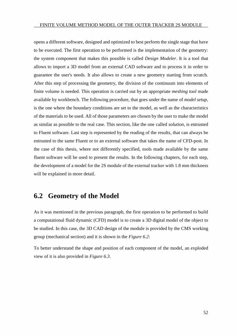
FINITE VOLUME METHOD MODEL OF THE OUTER TRACKER 2S MODULE
52
opens a different software, designed and optimized to best perform the single stage that have
to be executed. The first operation to be performed is the implementation of the geometry:
the system component that makes this possible is called Design Modeler. It is a tool that
allows to import a 3D model from an external CAD software and to process it in order to
guarantee the user's needs. It also allows to create a new geometry starting from scratch.
After this step of processing the geometry, the division of the continuum into elements of
finite volume is needed. This operation is carried out by an appropriate meshing tool made
available by workbench. The following procedure, that goes under the name of model setup,
is the one where the boundary conditions are set to the model, as well as the characteristics
of the materials to be used. All of those parameters are chosen by the user to make the model
as similar as possible to the real case. This section, like the one called solution, is entrusted
to Fluent software. Last step is represented by the reading of the results, that can always be
entrusted to the same Fluent or to an external software that takes the name of CFD-post. In
the case of this thesis, where not differently specified, tools made available by the same
fluent software will be used to present the results. In the following chapters, for each step,
the development of a model for the 2S module of the external tracker with 1.8 mm thickness
will be explained in more detail.
6.2 Geometry of the Model
As it was mentioned in the previous paragraph, the first operation to be performed to build
a computational fluid dynamic (CFD) model is to create a 3D digital model of the object to
be studied. In this case, the 3D CAD design of the module is provided by the CMS working
group (mechanical section) and it is shown in the Figure 6.2:
To better understand the shape and position of each component of the model, an exploded
view of it is also provided in Figure 6.3.
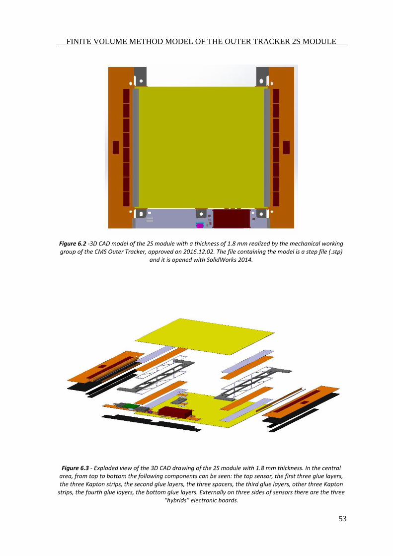
FINITE VOLUME METHOD MODEL OF THE OUTER TRACKER 2S MODULE
53
Figure 6.2 -3D CAD model of the 2S module with a thickness of 1.8 mm realized by the mechanical working group of the CMS Outer Tracker, approved on 2016.12.02. The file containing the model is a step file (.stp)
and it is opened with SolidWorks 2014.
Figure 6.3 - Exploded view of the 3D CAD drawing of the 2S module with 1.8 mm thickness. In the central area, from top to bottom the following components can be seen: the top sensor, the first three glue layers, the three Kapton strips, the second glue layers, the three spacers, the third glue layers, other three Kapton
strips, the fourth glue layers, the bottom glue layers. Externally on three sides of sensors there are the three “hybrids” electronic boards.
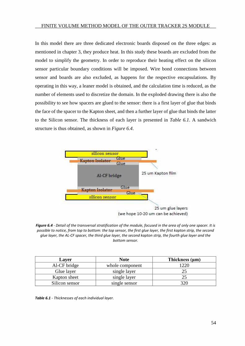
FINITE VOLUME METHOD MODEL OF THE OUTER TRACKER 2S MODULE
54
In this model there are three dedicated electronic boards disposed on the three edges: as
mentioned in chapter 3, they produce heat. In this study these boards are excluded from the
model to simplify the geometry. In order to reproduce their heating effect on the silicon
sensor particular boundary conditions will be imposed. Wire bond connections between
sensor and boards are also excluded, as happens for the respective encapsulations. By
operating in this way, a leaner model is obtained, and the calculation time is reduced, as the
number of elements used to discretize the domain. In the exploded drawing there is also the
possibility to see how spacers are glued to the sensor: there is a first layer of glue that binds
the face of the spacer to the Kapton sheet, and then a further layer of glue that binds the latter
to the Silicon sensor. The thickness of each layer is presented in Table 6.1. A sandwich
structure is thus obtained, as shown in Figure 6.4.
Figure 6.4 - Detail of the transversal stratification of the module, focused in the area of only one spacer. It is possible to notice, from top to bottom: the top sensor, the first glue layer, the first kapton strip, the second
glue layer, the AL-CF spacer, the third glue layer, the second kapton strip, the fourth glue layer and the bottom sensor.
Layer Note Thickness (μm)
Al-CF bridge whole component 1220
Glue layer single layer 25
Kapton sheet single layer 25
Silicon sensor single sensor 320
Table 6.1 - Thicknesses of each individual layer.

FINITE VOLUME METHOD MODEL OF THE OUTER TRACKER 2S MODULE
55
Glue and Kapton layers, as it will be seen in the next section, result very critical with regard
to the meshing phase. In fact, if they have to be divided into elements, they should have a
very high number of divisions, which make the numerical model considerably heavier.
However, they play a key role in thermal flux, since they introduce a non-negligible thermal
resistance, so they cannot be excluded from the model. Taking into account both these
reasons, the best way to treat these components is to physically exclude them from the
geometry, so as not to divide them into elements, and to simulate their effect with a contact
resistance, i.e. to introduce a mathematical relationship that can compensate for the choice
of exclusion. Therefore, the idea is to slice the model complete of layers, to cancel the 75
micrometres inclusive of the layer of the layer of the glue-kapton-glue, both on the top and
of the bottom of the Al-CF bridge, and to reattach the silicon directly to the spacer.
Looking again at the CAD drawing in Figure 6.2, if electronic boards are excluded, it appears
to be symmetrical with respect to a plane perpendicular to that on which the module lies, and
parallel to the two spacers. So the strategy of cutting the geometry of the module in half and
putting a symmetry plan on the cutting edge is adopted. In this way the number of elements
is halved, and the calculation times is lowered as the dimensions of the model are greatly
reduced. Another consideration to be made concerns the fluid that is present in the cavities
of the spacer: they are the chambers where the air is entrapped during assembly and remains
internally confined until the module enters into operative conditions as well as for the whole
life of it. Therefore, as it is generally air at atmospheric pressure, it is generally not
conductive, but since the layer is very thin, it gives a contribution to the thermal exchange
of interest. Moreover, between the two silicon plates, a fluid is present under operating
conditions (air or nitrogen): although this fluid is not able to develop a field of motion due
to natural convection, being the thickness being very thin so offering a contribution to the
exchange by conduction. The 3D CAD model does not foresee the physical presence of these
fluid layers between the components: for these reasons they are inserted in the Design
Modeler mode. At the end of this phase of geometry processing, the model appears as shown
in Figure 6.5:
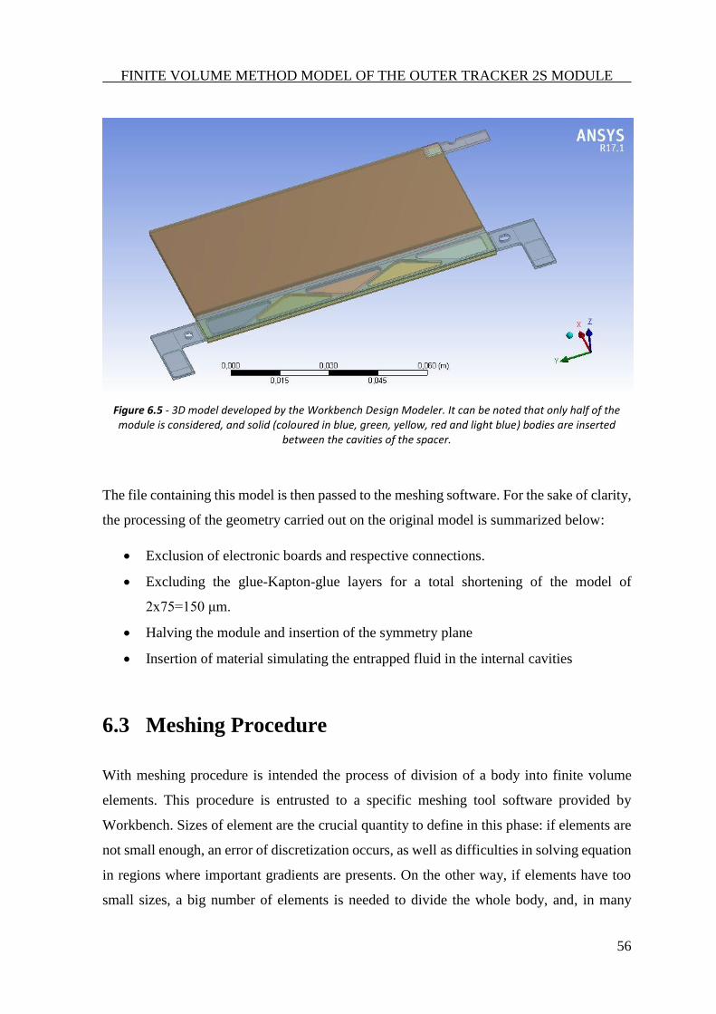
FINITE VOLUME METHOD MODEL OF THE OUTER TRACKER 2S MODULE
56
Figure 6.5 - 3D model developed by the Workbench Design Modeler. It can be noted that only half of the module is considered, and solid (coloured in blue, green, yellow, red and light blue) bodies are inserted
between the cavities of the spacer.
The file containing this model is then passed to the meshing software. For the sake of clarity,
the processing of the geometry carried out on the original model is summarized below:
• Exclusion of electronic boards and respective connections.
• Excluding the glue-Kapton-glue layers for a total shortening of the model of
2x75=150 μm.
• Halving the module and insertion of the symmetry plane
• Insertion of material simulating the entrapped fluid in the internal cavities
6.3 Meshing Procedure
With meshing procedure is intended the process of division of a body into finite volume
elements. This procedure is entrusted to a specific meshing tool software provided by
Workbench. Sizes of element are the crucial quantity to define in this phase: if elements are
not small enough, an error of discretization occurs, as well as difficulties in solving equation
in regions where important gradients are presents. On the other way, if elements have too
small sizes, a big number of elements is needed to divide the whole body, and, in many

FINITE VOLUME METHOD MODEL OF THE OUTER TRACKER 2S MODULE
57
cases, the power of the calculator may not be enough to handle the model. So it is necessary
to find the right compromise between times of calculation, power of the calculator, and level
of discretization of the model. Another factor to take in account during meshing operations
is the quality of each element. A square is an ideal geometrical shape, and error connected
in solving equations in this kind of volumes will be minimum. It follows from this that a
body has to be discretized in elements which shapes are much close to the ideal ideal. In
many practical cases, this is not achievable, because bodies have complex geometries, and
the only way is using volumes with not ideal shapes. The quantity called element quality
helps to judge how much elements are close to the shape of squares or cubes. The element
quality function of the Workbench meshing tool provides a composite quality metric that
ranges between 0 and 1. This metric is based on the ratio of the volume to the sum of the
square of the edge lengths for 2D quadrilateral or triangular elements, or the square root of
the cube of the sum of the square of the edge lengths for 3D elements. A value of 1 indicates
a perfect cube or square while a value of 0 indicates that the element has a zero or negative
volume. For three-dimensional brick elements:
𝑄𝑢𝑎𝑙𝑖𝑡𝑦 = 𝐶𝑣𝑜𝑙𝑢𝑚𝑒
√[∑(𝐸𝑑𝑔𝑒 𝐿𝑒𝑛𝑔ℎ𝑡)2]32 (6.1)
where C is a constant defined for each type of elements. After some attempts, the selected
value for elements medium size is imposed 1.21x10⁻⁴ m. The size function is computed when
meshing begins. When the Adaptive size function method is used, the mesher uses the value
of the Element seed size property to determine a starting point for the mesh size. The value
of the Element seed size property can be user-defined, or it can be automatically computed
by the mesher (defaulted based on the bounding box). When meshing begins, edges are
meshed with this size initially, and then they are refined for curvature and 2D proximity.
Next, mesh-based defeaturing occurs. The final edge mesh is then passed into a least-squares
fit size function, which guides face and volume meshing. For all other size function methods,
the mesher examines the size sources and, based on the smallest size obtained at the location
of the sources, the distance to each source, and the growth rate, the smallest size at each
point is selected and stored in a background grid. The mesher uses the sizes from the
background grid to generate a mesh. The background grid is refined automatically to provide
size distribution to the mesher. About the meshing procedure of the 2S module, the most
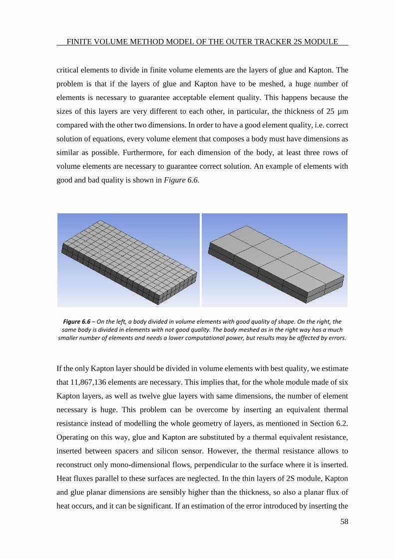
FINITE VOLUME METHOD MODEL OF THE OUTER TRACKER 2S MODULE
58
critical elements to divide in finite volume elements are the layers of glue and Kapton. The
problem is that if the layers of glue and Kapton have to be meshed, a huge number of
elements is necessary to guarantee acceptable element quality. This happens because the
sizes of this layers are very different to each other, in particular, the thickness of 25 µm
compared with the other two dimensions. In order to have a good element quality, i.e. correct
solution of equations, every volume element that composes a body must have dimensions as
similar as possible. Furthermore, for each dimension of the body, at least three rows of
volume elements are necessary to guarantee correct solution. An example of elements with
good and bad quality is shown in Figure 6.6.
Figure 6.6 – On the left, a body divided in volume elements with good quality of shape. On the right, the same body is divided in elements with not good quality. The body meshed as in the right way has a much
smaller number of elements and needs a lower computational power, but results may be affected by errors.
If the only Kapton layer should be divided in volume elements with best quality, we estimate
that 11,867,136 elements are necessary. This implies that, for the whole module made of six
Kapton layers, as well as twelve glue layers with same dimensions, the number of element
necessary is huge. This problem can be overcome by inserting an equivalent thermal
resistance instead of modelling the whole geometry of layers, as mentioned in Section 6.2.
Operating on this way, glue and Kapton are substituted by a thermal equivalent resistance,
inserted between spacers and silicon sensor. However, the thermal resistance allows to
reconstruct only mono-dimensional flows, perpendicular to the surface where it is inserted.
Heat fluxes parallel to these surfaces are neglected. In the thin layers of 2S module, Kapton
and glue planar dimensions are sensibly higher than the thickness, so also a planar flux of
heat occurs, and it can be significant. If an estimation of the error introduced by inserting the
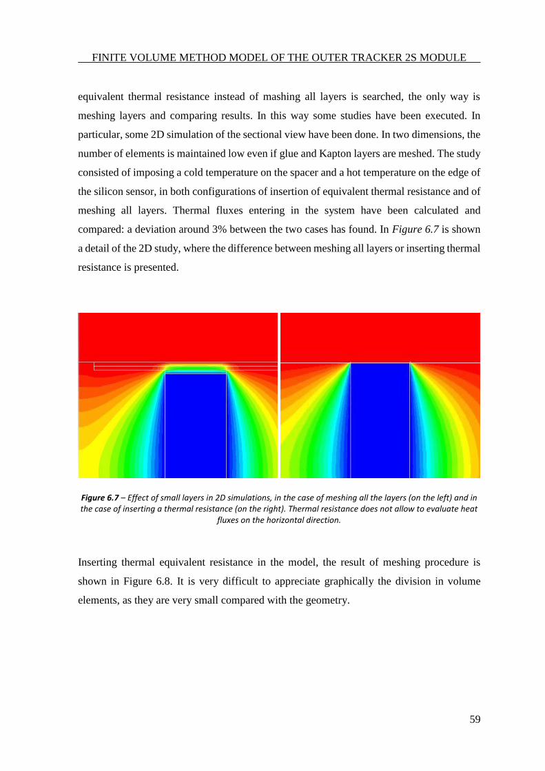
FINITE VOLUME METHOD MODEL OF THE OUTER TRACKER 2S MODULE
59
equivalent thermal resistance instead of mashing all layers is searched, the only way is
meshing layers and comparing results. In this way some studies have been executed. In
particular, some 2D simulation of the sectional view have been done. In two dimensions, the
number of elements is maintained low even if glue and Kapton layers are meshed. The study
consisted of imposing a cold temperature on the spacer and a hot temperature on the edge of
the silicon sensor, in both configurations of insertion of equivalent thermal resistance and of
meshing all layers. Thermal fluxes entering in the system have been calculated and
compared: a deviation around 3% between the two cases has found. In Figure 6.7 is shown
a detail of the 2D study, where the difference between meshing all layers or inserting thermal
resistance is presented.
Figure 6.7 – Effect of small layers in 2D simulations, in the case of meshing all the layers (on the left) and in the case of inserting a thermal resistance (on the right). Thermal resistance does not allow to evaluate heat
fluxes on the horizontal direction.
Inserting thermal equivalent resistance in the model, the result of meshing procedure is
shown in Figure 6.8. It is very difficult to appreciate graphically the division in volume
elements, as they are very small compared with the geometry.
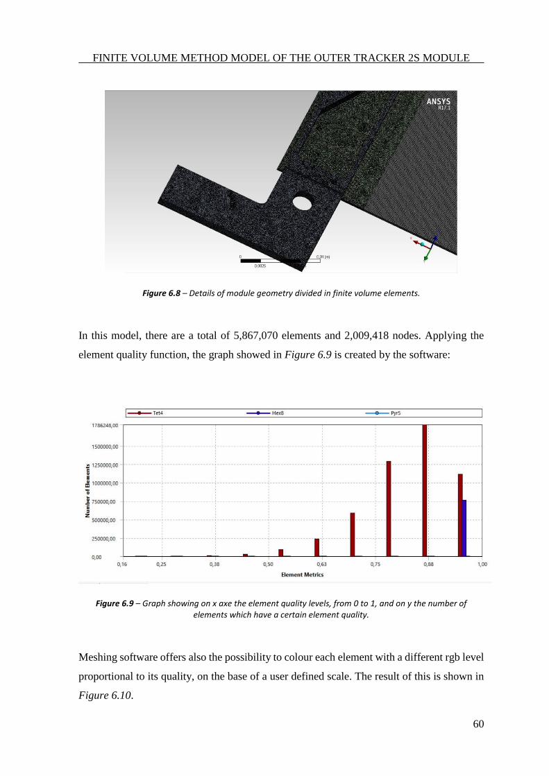
FINITE VOLUME METHOD MODEL OF THE OUTER TRACKER 2S MODULE
60
Figure 6.8 – Details of module geometry divided in finite volume elements.
In this model, there are a total of 5,867,070 elements and 2,009,418 nodes. Applying the
element quality function, the graph showed in Figure 6.9 is created by the software:
Figure 6.9 – Graph showing on x axe the element quality levels, from 0 to 1, and on y the number of elements which have a certain element quality.
Meshing software offers also the possibility to colour each element with a different rgb level
proportional to its quality, on the base of a user defined scale. The result of this is shown in
Figure 6.10.

FINITE VOLUME METHOD MODEL OF THE OUTER TRACKER 2S MODULE
61
Figure 6.10 – Volume elements coloured in different way as function of their element quality. Blue colour corresponds to a perfect quality.
6.4 Boundary Conditions
After meshing procedure, data have been loaded in Fluent solver. The first parameter to be
set in this ambient is the type of analysis that is wanted. In this case only a thermal analysis
is desired, and, as fluids in motion are not considered, the only equation to be solved is the
energy one. From this, it follows, considering also the steady state of the system, that the
only parameter characterising materials that is needed is the thermal conductivity. For solid
bodies, (silicon, spacers, air) values taken from Fluent database are used (see Table 6.2).
Material Thermal conductivity [W/mK]
Silicon 180
Aluminium 202.4
Air 0.0242
Table 6.2 – Material characteristics for materials.
For equivalent thermal resistances inserted in bodies interfaces (where needed), values are
calculated using equation (4.7). The software asks as input data the equivalent thermal
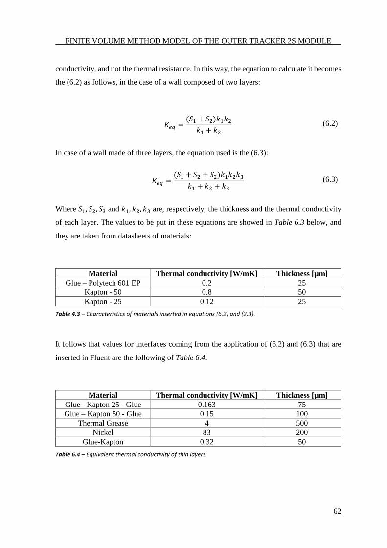
FINITE VOLUME METHOD MODEL OF THE OUTER TRACKER 2S MODULE
62
conductivity, and not the thermal resistance. In this way, the equation to calculate it becomes
the (6.2) as follows, in the case of a wall composed of two layers:
𝐾𝑒𝑞 =(𝑆1 + 𝑆2)𝑘1𝑘2
𝑘1 + 𝑘2 (6.2)
In case of a wall made of three layers, the equation used is the (6.3):
𝐾𝑒𝑞 =(𝑆1 + 𝑆2 + 𝑆2)𝑘1𝑘2𝑘3
𝑘1 + 𝑘2 + 𝑘3 (6.3)
Where 𝑆1, 𝑆2, 𝑆3 and 𝑘1, 𝑘2, 𝑘3 are, respectively, the thickness and the thermal conductivity
of each layer. The values to be put in these equations are showed in Table 6.3 below, and
they are taken from datasheets of materials:
Material Thermal conductivity [W/mK] Thickness [µm]
Glue – Polytech 601 EP 0.2 25
Kapton - 50 0.8 50
Kapton - 25 0.12 25
Table 4.3 – Characteristics of materials inserted in equations (6.2) and (2.3).
It follows that values for interfaces coming from the application of (6.2) and (6.3) that are
inserted in Fluent are the following of Table 6.4:
Material Thermal conductivity [W/mK] Thickness [µm]
Glue - Kapton 25 - Glue 0.163 75
Glue – Kapton 50 - Glue 0.15 100
Thermal Grease 4 500
Nickel 83 200
Glue-Kapton 0.32 50
Table 6.4 – Equivalent thermal conductivity of thin layers.
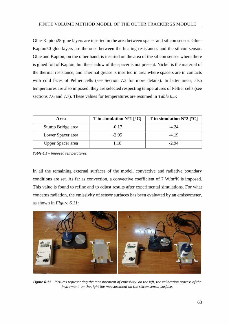
FINITE VOLUME METHOD MODEL OF THE OUTER TRACKER 2S MODULE
63
Glue-Kapton25-glue layers are inserted in the area between spacer and silicon sensor. Glue-
Kapton50-glue layers are the ones between the heating resistances and the silicon sensor.
Glue and Kapton, on the other hand, is inserted on the area of the silicon sensor where there
is glued foil of Kapton, but the shadow of the spacer is not present. Nickel is the material of
the thermal resistance, and Thermal grease is inserted in area where spacers are in contacts
with cold faces of Peltier cells (see Section 7.3 for more details). In latter areas, also
temperatures are also imposed: they are selected respecting temperatures of Peltier cells (see
sections 7.6 and 7.7). These values for temperatures are resumed in Table 6.5:
Area T in simulation N°1 [°C] T in simulation N°2 [°C]
Stump Bridge area -0.17 -4.24
Lower Spacer area -2.95 -4.19
Upper Spacer area 1.18 -2.94
Table 6.5 – Imposed temperatures.
In all the remaining external surfaces of the model, convective and radiative boundary
conditions are set. As far as convection, a convective coefficient of 7 W/m2K is imposed.
This value is found to refine and to adjust results after experimental simulations. For what
concerns radiation, the emissivity of sensor surfaces has been evaluated by an emissometer,
as shown in Figure 6.11:
Figure 6.11 – Pictures representing the measurement of emissivity: on the left, the calibration process of the instrument, on the right the measurement on the silicon sensor surface.
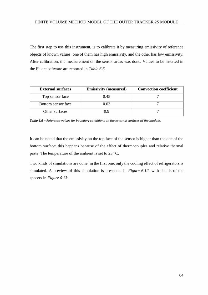
FINITE VOLUME METHOD MODEL OF THE OUTER TRACKER 2S MODULE
64
The first step to use this instrument, is to calibrate it by measuring emissivity of reference
objects of known values: one of them has high emissivity, and the other has low emissivity.
After calibration, the measurement on the sensor areas was done. Values to be inserted in
the Fluent software are reported in Table 6.6.
External surfaces Emissivity (measured) Convection coefficient
Top sensor face 0.45 7
Bottom sensor face 0.03 7
Other surfaces 0.9 7
Table 6.6 – Reference values for boundary conditions on the external surfaces of the module.
It can be noted that the emissivity on the top face of the sensor is higher than the one of the
bottom surface: this happens because of the effect of thermocouples and relative thermal
paste. The temperature of the ambient is set to 23 °C.
Two kinds of simulations are done: in the first one, only the cooling effect of refrigerators is
simulated. A preview of this simulation is presented in Figure 6.12, with details of the
spacers in Figure 6.13:
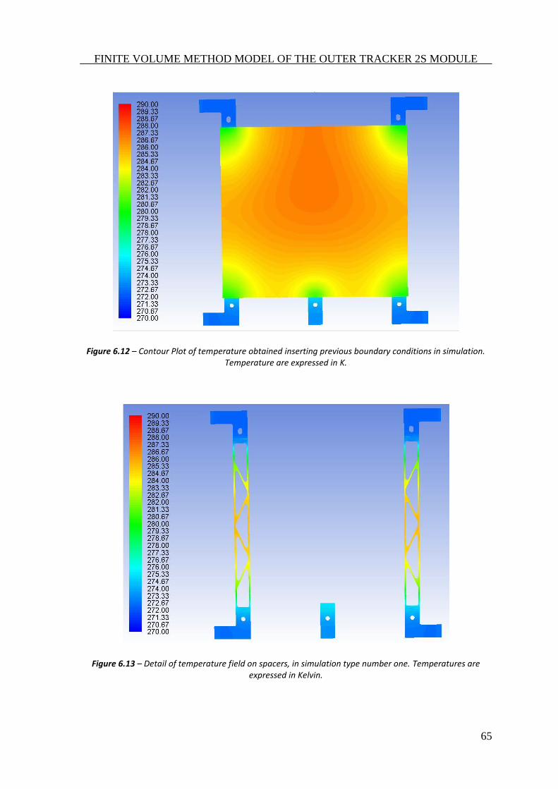
FINITE VOLUME METHOD MODEL OF THE OUTER TRACKER 2S MODULE
65
Figure 6.12 – Contour Plot of temperature obtained inserting previous boundary conditions in simulation. Temperature are expressed in K.
Figure 6.13 – Detail of temperature field on spacers, in simulation type number one. Temperatures are expressed in Kelvin.
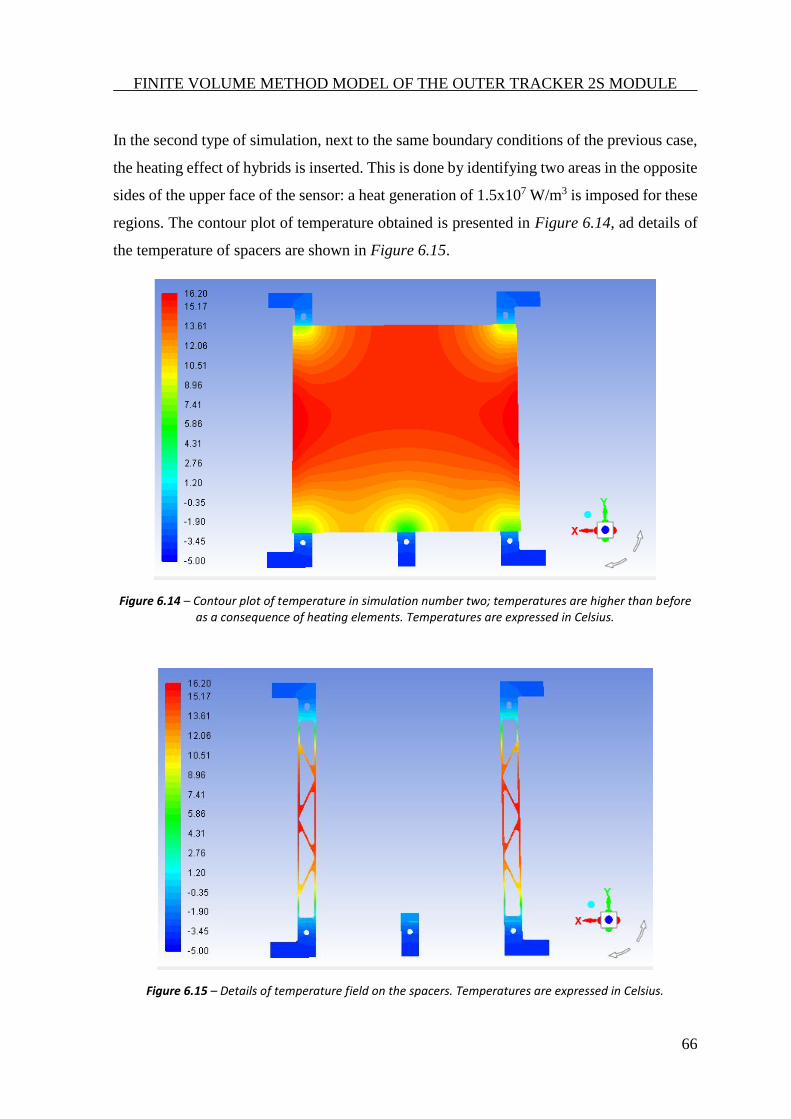
FINITE VOLUME METHOD MODEL OF THE OUTER TRACKER 2S MODULE
66
In the second type of simulation, next to the same boundary conditions of the previous case,
the heating effect of hybrids is inserted. This is done by identifying two areas in the opposite
sides of the upper face of the sensor: a heat generation of 1.5x10⁷ W/m3 is imposed for these
regions. The contour plot of temperature obtained is presented in Figure 6.14, ad details of
the temperature of spacers are shown in Figure 6.15.
Figure 6.14 – Contour plot of temperature in simulation number two; temperatures are higher than before as a consequence of heating elements. Temperatures are expressed in Celsius.
Figure 6.15 – Details of temperature field on the spacers. Temperatures are expressed in Celsius.
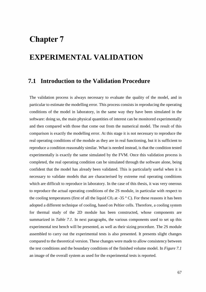
67
Chapter 7
EXPERIMENTAL VALIDATION
7.1 Introduction to the Validation Procedure
The validation process is always necessary to evaluate the quality of the model, and in
particular to estimate the modelling error. This process consists in reproducing the operating
conditions of the model in laboratory, in the same way they have been simulated in the
software: doing so, the main physical quantities of interest can be monitored experimentally
and then compared with those that come out from the numerical model. The result of this
comparison is exactly the modelling error. At this stage it is not necessary to reproduce the
real operating conditions of the module as they are in real functioning, but it is sufficient to
reproduce a condition reasonably similar. What is needed instead, is that the condition tested
experimentally is exactly the same simulated by the FVM. Once this validation process is
completed, the real operating condition can be simulated through the software alone, being
confident that the model has already been validated. This is particularly useful when it is
necessary to validate models that are characterised by extreme real operating conditions
which are difficult to reproduce in laboratory. In the case of this thesis, it was very onerous
to reproduce the actual operating conditions of the 2S module, in particular with respect to
the cooling temperatures (first of all the liquid C02 at -35 ° C). For these reasons it has been
adopted a different technique of cooling, based on Peltier cells. Therefore, a cooling system
for thermal study of the 2D module has been constructed, whose components are
summarized in Table 7.1. In next paragraphs, the various components used to set up this
experimental test bench will be presented, as well as their sizing procedure. The 2S module
assembled to carry out the experimental tests is also presented. It presents slight changes
compared to the theoretical version. These changes were made to allow consistency between
the test conditions and the boundary conditions of the finished volume model. In Figure 7.1
an image of the overall system as used for the experimental tests is reported.
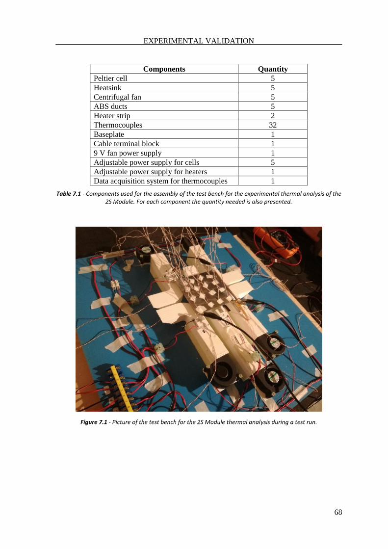
EXPERIMENTAL VALIDATION
68
Components Quantity
Peltier cell 5
Heatsink 5
Centrifugal fan 5
ABS ducts 5
Heater strip 2
Thermocouples 32
Baseplate 1
Cable terminal block 1
9 V fan power supply 1
Adjustable power supply for cells 5
Adjustable power supply for heaters 1
Data acquisition system for thermocouples 1
Table 7.1 - Components used for the assembly of the test bench for the experimental thermal analysis of the 2S Module. For each component the quantity needed is also presented.
Figure 7.1 - Picture of the test bench for the 2S Module thermal analysis during a test run.
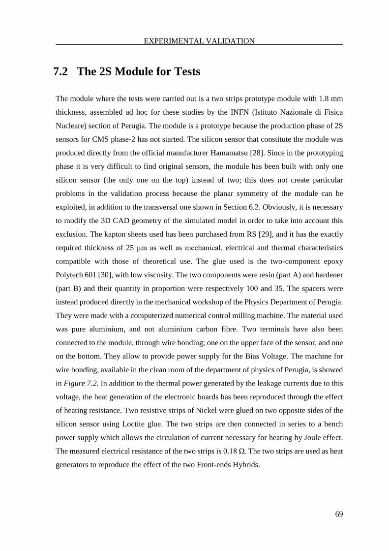
EXPERIMENTAL VALIDATION
69
7.2 The 2S Module for Tests
The module where the tests were carried out is a two strips prototype module with 1.8 mm
thickness, assembled ad hoc for these studies by the INFN (Istituto Nazionale di Fisica
Nucleare) section of Perugia. The module is a prototype because the production phase of 2S
sensors for CMS phase-2 has not started. The silicon sensor that constitute the module was
produced directly from the official manufacturer Hamamatsu [28]. Since in the prototyping
phase it is very difficult to find original sensors, the module has been built with only one
silicon sensor (the only one on the top) instead of two; this does not create particular
problems in the validation process because the planar symmetry of the module can be
exploited, in addition to the transversal one shown in Section 6.2. Obviously, it is necessary
to modify the 3D CAD geometry of the simulated model in order to take into account this
exclusion. The kapton sheets used has been purchased from RS [29], and it has the exactly
required thickness of 25 μm as well as mechanical, electrical and thermal characteristics
compatible with those of theoretical use. The glue used is the two-component epoxy
Polytech 601 [30], with low viscosity. The two components were resin (part A) and hardener
(part B) and their quantity in proportion were respectively 100 and 35. The spacers were
instead produced directly in the mechanical workshop of the Physics Department of Perugia.
They were made with a computerized numerical control milling machine. The material used
was pure aluminium, and not aluminium carbon fibre. Two terminals have also been
connected to the module, through wire bonding; one on the upper face of the sensor, and one
on the bottom. They allow to provide power supply for the Bias Voltage. The machine for
wire bonding, available in the clean room of the department of physics of Perugia, is showed
in Figure 7.2. In addition to the thermal power generated by the leakage currents due to this
voltage, the heat generation of the electronic boards has been reproduced through the effect
of heating resistance. Two resistive strips of Nickel were glued on two opposite sides of the
silicon sensor using Loctite glue. The two strips are then connected in series to a bench
power supply which allows the circulation of current necessary for heating by Joule effect.
The measured electrical resistance of the two strips is 0.18 Ω. The two strips are used as heat
generators to reproduce the effect of the two Front-ends Hybrids.
EXPERIMENTAL VALIDATION
70
Figure 7.2 – On the left the wire bonding machine of the Perugia INFN section laboratory used to connect the strips of the silicon sensor to the Bias Voltage Pins. On the right the silicon module for tests is presented.
These are in fact connected to the module by wire bonding and encapsulation, and then
provide a bridge for the heat to move from the board to the silicon. The Service Hybrid is
not directly connected to silicon with wire bonding, so no heat source has been arranged to
reproduce its effect. To ensure electrical insulation between the heating strip and the upper
face of the sensor, a strip of 50 µm thickness Kapton is inserted between the two. A new
“sandwich“ structure made by glue, Kapton and glue is then created.
7.3 Peltier Cells
Peltier cells are thermoelectric devices. The thermoelectric effect is the direct conversion of
temperature difference to electric voltage and vice versa. A thermoelectric device creates
voltage when there is a different temperature on each side. Conversely, when a voltage is
applied to it, it creates a temperature difference [23]. The thermoelectric effect therefore
includes three different physical phenomena that go under the name, respectively, of
Seebeck effect, Peltier effect, and Thomson effect. We have the first effect when we join
two dissimilar metals in two different points, and we put them at different temperatures:
inside the circuit formed by the two metals will flow an electric current. This principle is
used for the construction of thermocouples. We have the Thomson effect when an electric
current is passed through a conductor having a temperature gradient over its length: heat will
be either absorbed by or expelled from the conductor. The Peltier effect, on the other hand,
mirrors the Seebeck effect, and it occurs when a current flow in a circuit consisting of two
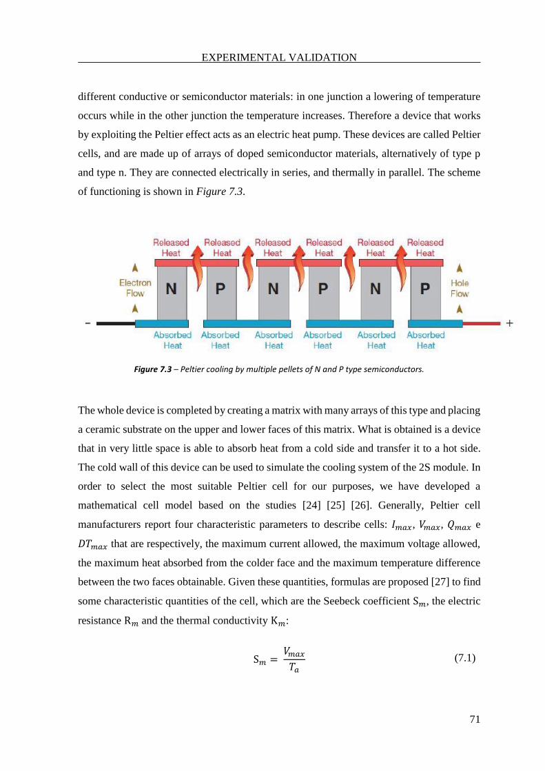
EXPERIMENTAL VALIDATION
71
different conductive or semiconductor materials: in one junction a lowering of temperature
occurs while in the other junction the temperature increases. Therefore a device that works
by exploiting the Peltier effect acts as an electric heat pump. These devices are called Peltier
cells, and are made up of arrays of doped semiconductor materials, alternatively of type p
and type n. They are connected electrically in series, and thermally in parallel. The scheme
of functioning is shown in Figure 7.3.
Figure 7.3 – Peltier cooling by multiple pellets of N and P type semiconductors.
The whole device is completed by creating a matrix with many arrays of this type and placing
a ceramic substrate on the upper and lower faces of this matrix. What is obtained is a device
that in very little space is able to absorb heat from a cold side and transfer it to a hot side.
The cold wall of this device can be used to simulate the cooling system of the 2S module. In
order to select the most suitable Peltier cell for our purposes, we have developed a
mathematical cell model based on the studies [24] [25] [26]. Generally, Peltier cell
manufacturers report four characteristic parameters to describe cells: 𝐼𝑚𝑎𝑥, 𝑉𝑚𝑎𝑥, 𝑄𝑚𝑎𝑥 e
𝐷𝑇𝑚𝑎𝑥 that are respectively, the maximum current allowed, the maximum voltage allowed,
the maximum heat absorbed from the colder face and the maximum temperature difference
between the two faces obtainable. Given these quantities, formulas are proposed [27] to find
some characteristic quantities of the cell, which are the Seebeck coefficient S𝑚, the electric
resistance R𝑚 and the thermal conductivity K𝑚:
S𝑚 = 𝑉𝑚𝑎𝑥
𝑇𝑎 (7.1)
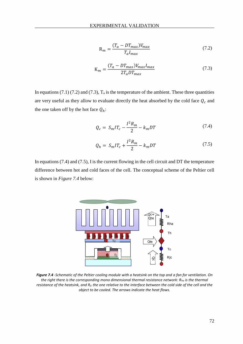
EXPERIMENTAL VALIDATION
72
R𝑚 =(𝑇𝑎 − 𝐷𝑇𝑚𝑎𝑥)𝑉𝑚𝑎𝑥
𝑇𝑎𝐼𝑚𝑎𝑥 (7.2)
K𝑚 =(𝑇𝑎 − 𝐷𝑇𝑚𝑎𝑥)𝑉𝑚𝑎𝑥𝐼𝑚𝑎𝑥
2𝑇𝑎𝐷𝑇𝑚𝑎𝑥 (7.3)
In equations (7.1) (7.2) and (7.3), Ta is the temperature of the ambient. These three quantities
are very useful as they allow to evaluate directly the heat absorbed by the cold face 𝑄𝑐 and
the one taken off by the hot face 𝑄ℎ:
𝑄𝑐 = 𝑆𝑚𝐼𝑇𝑐 −𝐼2𝑅𝑚
2− 𝑘𝑚𝐷𝑇 (7.4)
𝑄ℎ = 𝑆𝑚𝐼𝑇𝑐 +𝐼2𝑅𝑚
2− 𝑘𝑚𝐷𝑇 (7.5)
In equations (7.4) and (7.5), I is the current flowing in the cell circuit and DT the temperature
difference between hot and cold faces of the cell. The conceptual scheme of the Peltier cell
is shown in Figure 7.4 below:
Figure 7.4 -Schematic of the Peltier cooling module with a heatsink on the top and a fan for ventilation. On the right there is the corresponding mono dimensional thermal resistance network: Rha is the thermal
resistance of the heatsink, and Rjc the one relative to the interface between the cold side of the cell and the object to be cooled. The arrows indicate the heat flows.
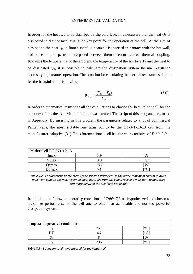
EXPERIMENTAL VALIDATION
73
In order for the heat Qc to be absorbed by the cold face, it is necessary that the heat Qh is
dissipated in the hot face: this is the key point for the operation of the cell. At the aim of
dissipating the heat Qc, a finned metallic heatsink is inserted in contact with the hot wall,
and some thermal paste is interposed between them to ensure correct thermal coupling.
Knowing the temperature of the ambient, the temperature of the hot face Th and the heat to
be dissipated Qc, it is possible to calculate the dissipation system thermal resistance
necessary to guarantee operation. The equation for calculating the thermal resistance suitable
for the heatsink is the following:
Rℎ𝑎 =(𝑇ℎ − 𝑇𝑎)
𝑄ℎ
(7.6)
In order to automatically manage all the calculations to choose the best Peltier cell for the
purposes of this thesis, a Matlab program was created. The script of this program is reported
in Appendix. By inserting in this program the parameters related to a lot of commercial
Peltier cells, the most suitable one turns out to be the ET-071-10-13 cell from the
manufacturer Adaptive [31]. The aforementioned cell has the characteristics of Table 7.2:
Peltier Cell ET-071-10-13
Imax 3.9 [A]
Vmax 8.8 [V]
Qcmax 18.7 [W]
DTmax 74 [°C]
Table 7.2 - Characteristic parameters of the selected Peltier cell, in the order: maximum current allowed, maximum voltage allowed, maximum heat absorbed from the colder face and maximum temperature
difference between the two faces obtainable
In addition, the following operating conditions of Table 7.3 are hypothesized and chosen to
maximize performance of the cell and to obtain an achievable and not too powerful
dissipation system:
Imposed operative conditions
Tc 267 [°C]
DT 46 [°C]
Qc 5 [W]
Ta 296 [°C]
Table 7.3 – Boundary conditions imposed for the Peltier cell
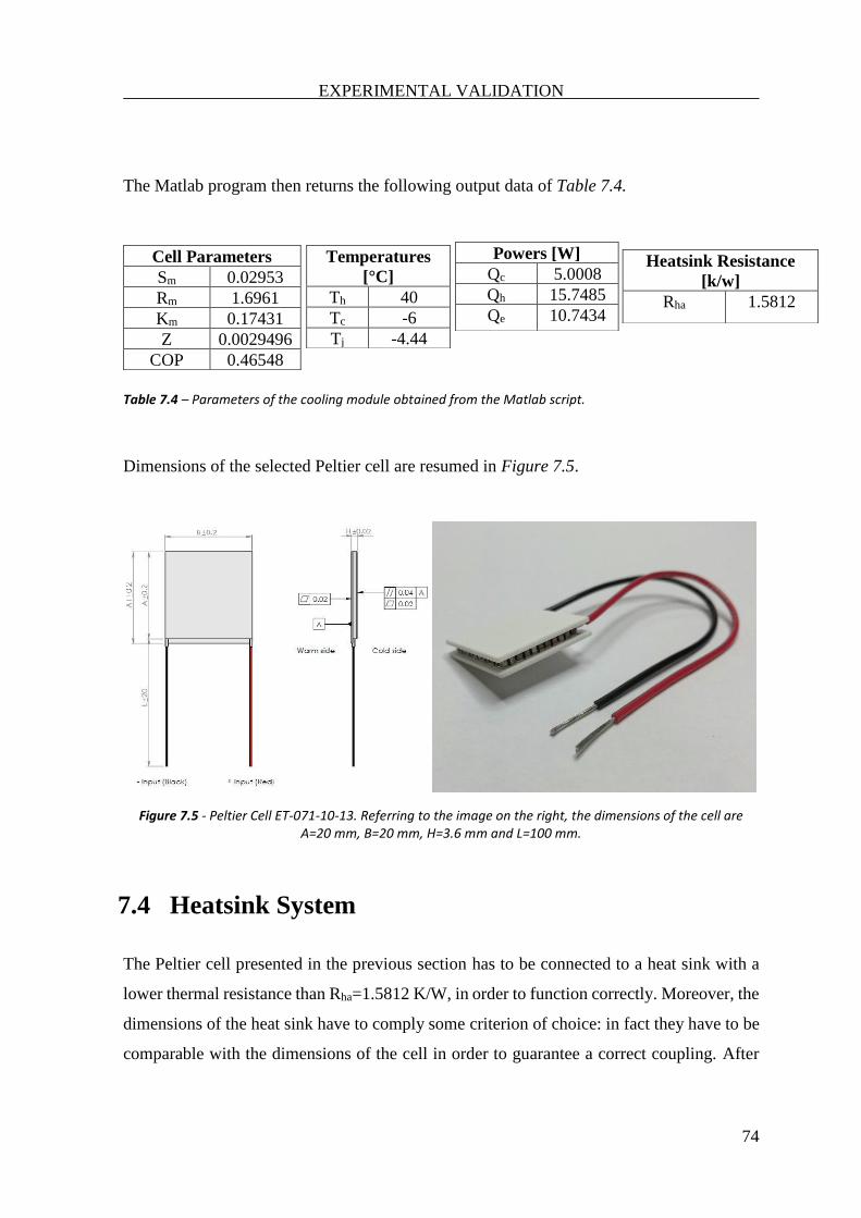
EXPERIMENTAL VALIDATION
74
The Matlab program then returns the following output data of Table 7.4.
Table 7.4 – Parameters of the cooling module obtained from the Matlab script.
Dimensions of the selected Peltier cell are resumed in Figure 7.5.
Figure 7.5 - Peltier Cell ET-071-10-13. Referring to the image on the right, the dimensions of the cell are A=20 mm, B=20 mm, H=3.6 mm and L=100 mm.
7.4 Heatsink System
The Peltier cell presented in the previous section has to be connected to a heat sink with a
lower thermal resistance than Rha=1.5812 K/W, in order to function correctly. Moreover, the
dimensions of the heat sink have to comply some criterion of choice: in fact they have to be
comparable with the dimensions of the cell in order to guarantee a correct coupling. After
Cell Parameters
Sm 0.02953
Rm 1.6961
Km 0.17431
Z 0.0029496
COP 0.46548
Temperatures
[°C]
Th 40
Tc -6
Tj -4.44
Powers [W]
Qc 5.0008
Qh 15.7485
Qe 10.7434
Heatsink Resistance
[k/w]
Rha 1.5812
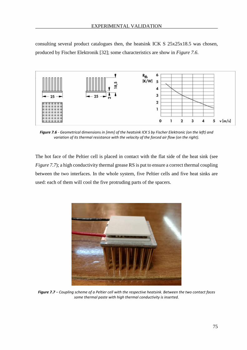
EXPERIMENTAL VALIDATION
75
consulting several product catalogues then, the heatsink ICK S 25x25x18.5 was chosen,
produced by Fischer Elektronik [32]; some characteristics are show in Figure 7.6.
Figure 7.6 - Geometrical dimensions in [mm] of the heatsink ICK S by Fischer Elektronic (on the left) and variation of its thermal resistance with the velocity of the forced air flow (on the right).
The hot face of the Peltier cell is placed in contact with the flat side of the heat sink (see
Figure 7.7); a high conductivity thermal grease RS is put to ensure a correct thermal coupling
between the two interfaces. In the whole system, five Peltier cells and five heat sinks are
used: each of them will cool the five protruding parts of the spacers.
Figure 7.7 – Coupling scheme of a Peltier cell with the respective heatsink. Between the two contact faces some thermal paste with high thermal conductivity is inserted.
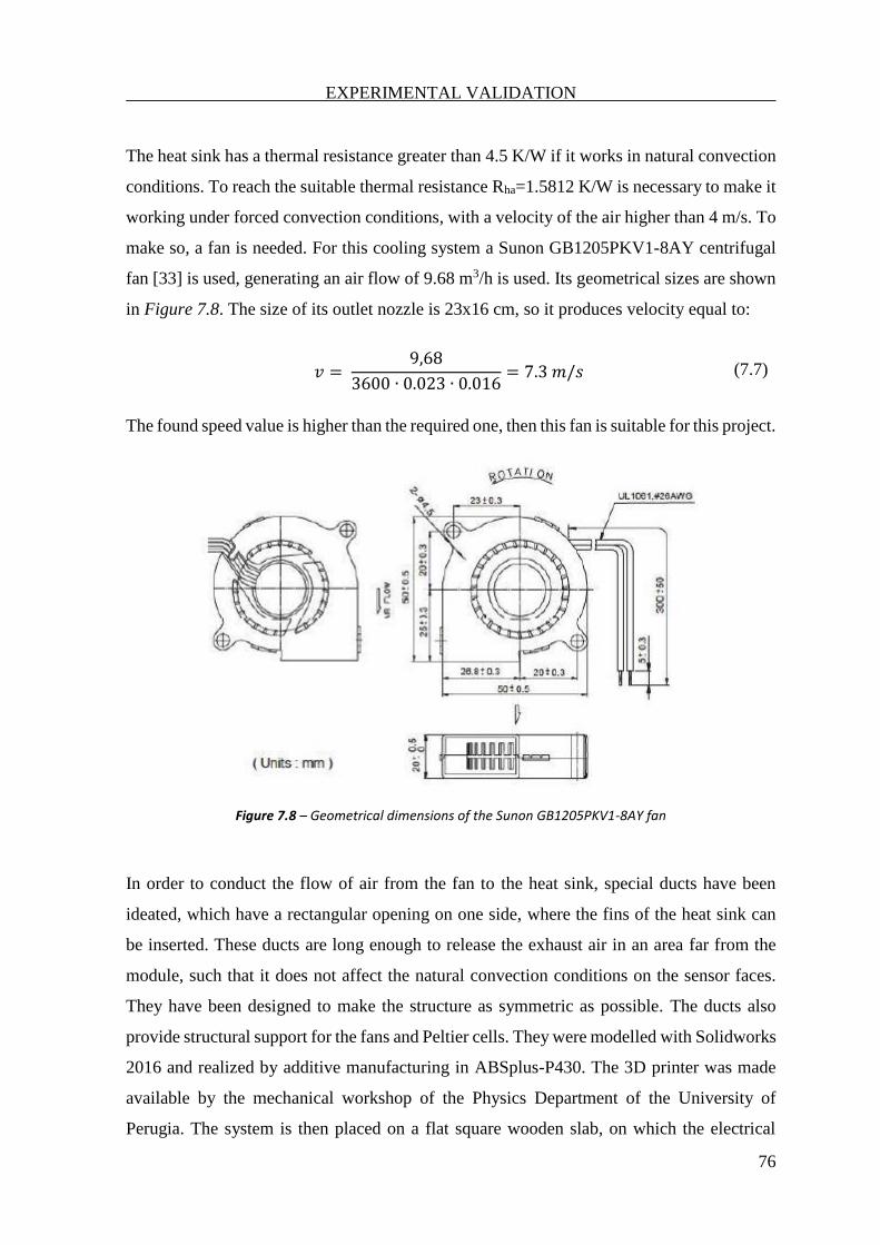
EXPERIMENTAL VALIDATION
76
The heat sink has a thermal resistance greater than 4.5 K/W if it works in natural convection
conditions. To reach the suitable thermal resistance Rha=1.5812 K/W is necessary to make it
working under forced convection conditions, with a velocity of the air higher than 4 m/s. To
make so, a fan is needed. For this cooling system a Sunon GB1205PKV1-8AY centrifugal
fan [33] is used, generating an air flow of 9.68 m3/h is used. Its geometrical sizes are shown
in Figure 7.8. The size of its outlet nozzle is 23x16 cm, so it produces velocity equal to:
𝑣 = 9,68
3600 ∙ 0.023 ∙ 0.016= 7.3 𝑚/𝑠 (7.7)
The found speed value is higher than the required one, then this fan is suitable for this project.
Figure 7.8 – Geometrical dimensions of the Sunon GB1205PKV1-8AY fan
In order to conduct the flow of air from the fan to the heat sink, special ducts have been
ideated, which have a rectangular opening on one side, where the fins of the heat sink can
be inserted. These ducts are long enough to release the exhaust air in an area far from the
module, such that it does not affect the natural convection conditions on the sensor faces.
They have been designed to make the structure as symmetric as possible. The ducts also
provide structural support for the fans and Peltier cells. They were modelled with Solidworks
2016 and realized by additive manufacturing in ABSplus-P430. The 3D printer was made
available by the mechanical workshop of the Physics Department of the University of
Perugia. The system is then placed on a flat square wooden slab, on which the electrical
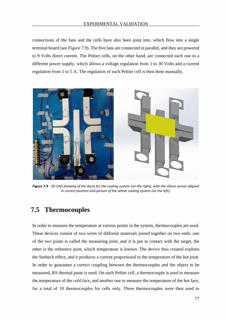
EXPERIMENTAL VALIDATION
77
connections of the fans and the cells have also been joint into, which flow into a single
terminal board (see Figure 7.9). The five fans are connected in parallel, and they are powered
to 9 Volts direct current. The Peltier cells, on the other hand, are connected each one to a
different power supply, which allows a voltage regulation from 1 to 30 Volts and a current
regulation from 1 to 5 A. The regulation of each Peltier cell is then done manually.
Figure 7.9 - 3D CAD drawing of the ducts for the cooling system (on the right), with the silicon sensor aligned in correct position and picture of the whole cooling system (on the left).
7.5 Thermocouples
In order to measure the temperature at various points in the system, thermocouples are used.
These devices consist of two wires of different materials joined together on two ends: one
of the two joints is called the measuring joint, and it is put in contact with the target, the
other is the reference joint, which temperature is known. The device thus created exploits
the Seebeck effect, and it produces a current proportional to the temperature of the hot joint.
In order to guarantee a correct coupling between the thermocouples and the object to be
measured, RS thermal paste is used. On each Peltier cell, a thermocouple is used to measure
the temperature of the cold face, and another one to measure the temperature of the hot face,
for a total of 10 thermocouples for cells only. Three thermocouples were then used to
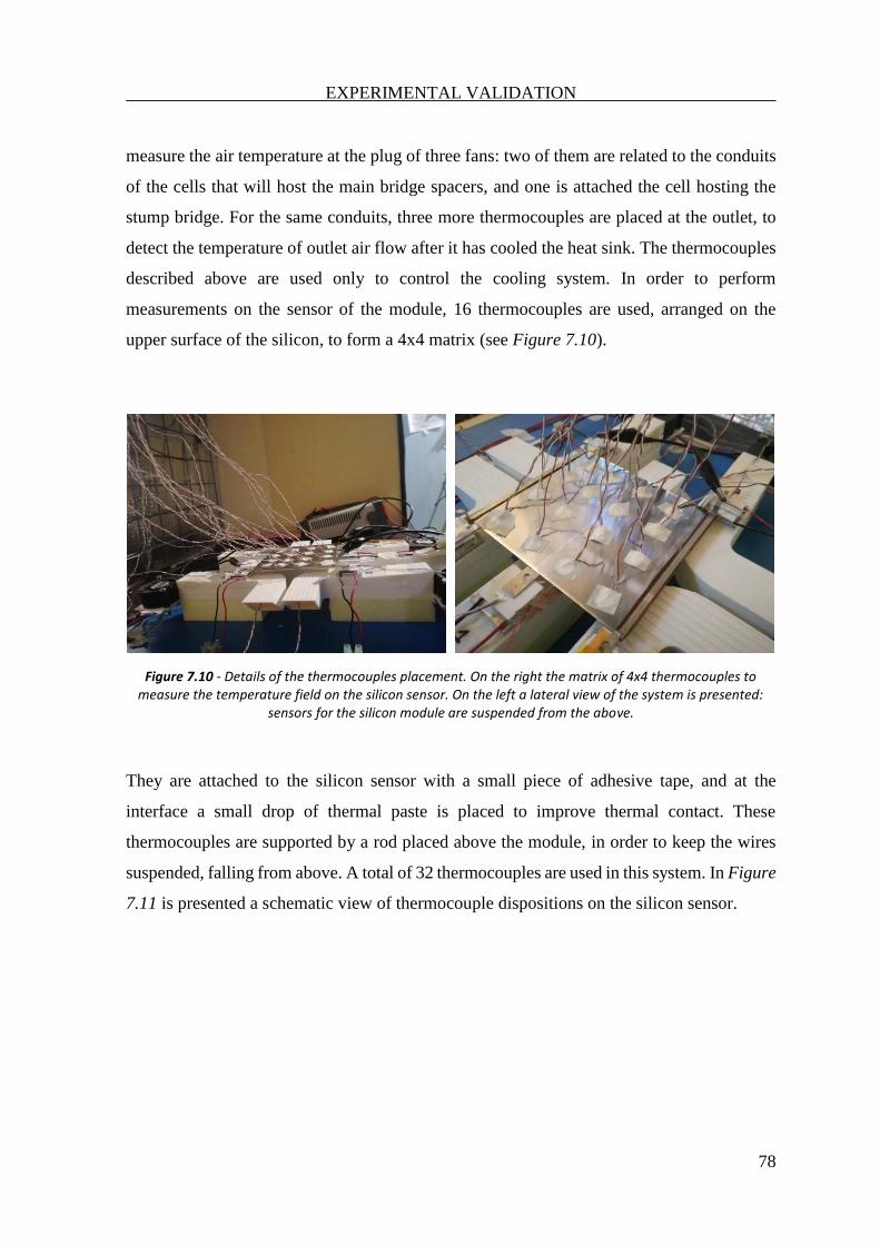
EXPERIMENTAL VALIDATION
78
measure the air temperature at the plug of three fans: two of them are related to the conduits
of the cells that will host the main bridge spacers, and one is attached the cell hosting the
stump bridge. For the same conduits, three more thermocouples are placed at the outlet, to
detect the temperature of outlet air flow after it has cooled the heat sink. The thermocouples
described above are used only to control the cooling system. In order to perform
measurements on the sensor of the module, 16 thermocouples are used, arranged on the
upper surface of the silicon, to form a 4x4 matrix (see Figure 7.10).
Figure 7.10 - Details of the thermocouples placement. On the right the matrix of 4x4 thermocouples to measure the temperature field on the silicon sensor. On the left a lateral view of the system is presented:
sensors for the silicon module are suspended from the above.
They are attached to the silicon sensor with a small piece of adhesive tape, and at the
interface a small drop of thermal paste is placed to improve thermal contact. These
thermocouples are supported by a rod placed above the module, in order to keep the wires
suspended, falling from above. A total of 32 thermocouples are used in this system. In Figure
7.11 is presented a schematic view of thermocouple dispositions on the silicon sensor.
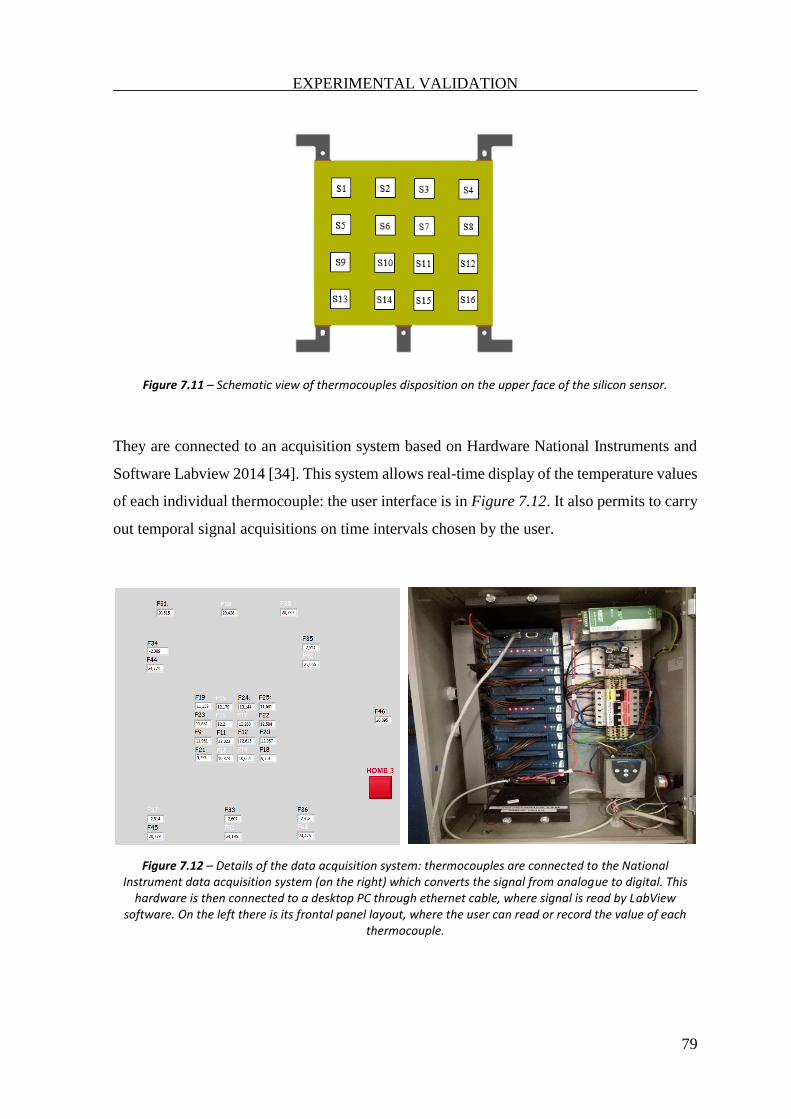
EXPERIMENTAL VALIDATION
79
Figure 7.11 – Schematic view of thermocouples disposition on the upper face of the silicon sensor.
They are connected to an acquisition system based on Hardware National Instruments and
Software Labview 2014 [34]. This system allows real-time display of the temperature values
of each individual thermocouple: the user interface is in Figure 7.12. It also permits to carry
out temporal signal acquisitions on time intervals chosen by the user.
Figure 7.12 – Details of the data acquisition system: thermocouples are connected to the National Instrument data acquisition system (on the right) which converts the signal from analogue to digital. This
hardware is then connected to a desktop PC through ethernet cable, where signal is read by LabView software. On the left there is its frontal panel layout, where the user can read or record the value of each
thermocouple.
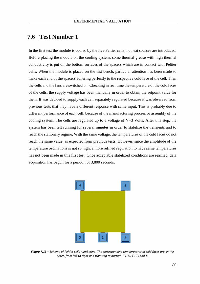
EXPERIMENTAL VALIDATION
80
7.6 Test Number 1
In the first test the module is cooled by the five Peltier cells; no heat sources are introduced.
Before placing the module on the cooling system, some thermal grease with high thermal
conductivity is put on the bottom surfaces of the spacers which are in contact with Peltier
cells. When the module is placed on the test bench, particular attention has been made to
make each end of the spacers adhering perfectly to the respective cold face of the cell. Then
the cells and the fans are switched on. Checking in real time the temperature of the cold faces
of the cells, the supply voltage has been manually in order to obtain the setpoint value for
them. It was decided to supply each cell separately regulated because it was observed from
previous tests that they have a different response with same input. This is probably due to
different performance of each cell, because of the manufacturing process or assembly of the
cooling system. The cells are regulated up to a voltage of V=3 Volts. After this step, the
system has been left running for several minutes in order to stabilize the transients and to
reach the stationary regime. With the same voltage, the temperatures of the cold faces do not
reach the same value, as expected from previous tests. However, since the amplitude of the
temperature oscillations is not so high, a more refined regulation to have same temperatures
has not been made in this first test. Once acceptable stabilized conditions are reached, data
acquisition has begun for a period t of 3,800 seconds.
Figure 7.13 – Scheme of Peltier cells numbering. The corresponding temperatures of cold faces are, in the order, from left to right and from top to bottom: T4, T2, T5, T1 and T3
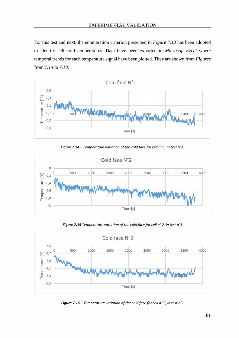
EXPERIMENTAL VALIDATION
81
For this test and next, the enumeration criterion presented in Figure 7.13 has been adopted
to identify cell cold temperatures. Data have been exported to Microsoft Excel where
temporal trends for each temperature signal have been plotted. They are shown from Figures
from 7.14 to 7.18.
Figure 7.14 – Temperature variation of the cold face for cell n° 1, in test n°1.
Figure 7.15 Temperature variation of the cold face for cell n° 2, in test n°1
Figure 7.16 – Temperature variation of the cold face for cell n° 3, in test n°1
-0,5
-0,3
-0,1
0,1
0,3
0,5
0 500 1000 1500 2000 2500 3000 3500 4000
Tem
per
atu
re [
°C]
Time [s]
Cold face N°1
-1
-0,8
-0,6
-0,4
-0,2
0
0 500 1000 1500 2000 2500 3000 3500 4000
Tem
per
atu
re [
°C]
Time [s]
Cold face N°2
-3,5
-3,3
-3,1
-2,9
-2,7
-2,5
0 500 1000 1500 2000 2500 3000 3500 4000
Tem
per
atu
re [
°C]
Time [s]
Cold face N°3
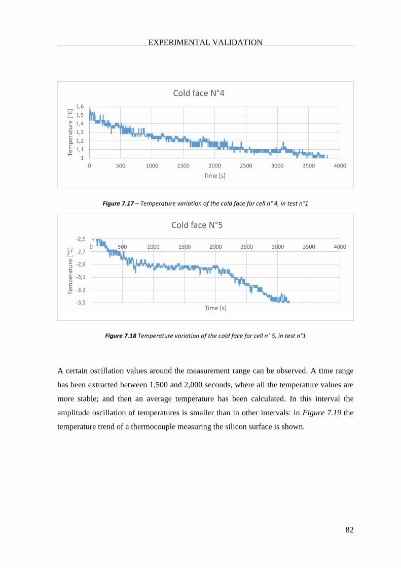
EXPERIMENTAL VALIDATION
82
Figure 7.17 – Temperature variation of the cold face for cell n° 4, in test n°1
Figure 7.18 Temperature variation of the cold face for cell n° 5, in test n°1
A certain oscillation values around the measurement range can be observed. A time range
has been extracted between 1,500 and 2,000 seconds, where all the temperature values are
more stable; and then an average temperature has been calculated. In this interval the
amplitude oscillation of temperatures is smaller than in other intervals: in Figure 7.19 the
temperature trend of a thermocouple measuring the silicon surface is shown.
1
1,1
1,2
1,3
1,4
1,5
1,6
0 500 1000 1500 2000 2500 3000 3500 4000
Tem
per
atu
re [
°C]
Time [s]
Cold face N°4
-3,5
-3,3
-3,1
-2,9
-2,7
-2,5
0 500 1000 1500 2000 2500 3000 3500 4000
Tem
per
atu
re [
°C]
Time [s]
Cold face N°5
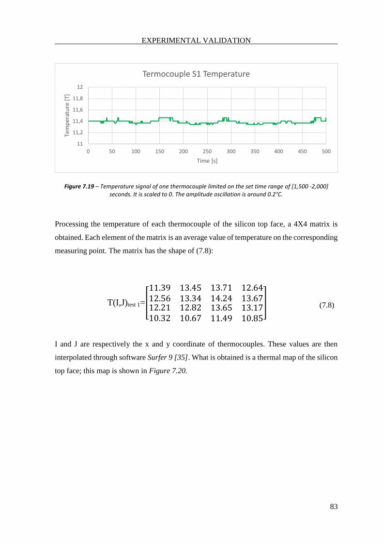
EXPERIMENTAL VALIDATION
83
Figure 7.19 – Temperature signal of one thermocouple limited on the set time range of [1,500 -2,000] seconds. It is scaled to 0. The amplitude oscillation is around 0.2°C.
Processing the temperature of each thermocouple of the silicon top face, a 4X4 matrix is
obtained. Each element of the matrix is an average value of temperature on the corresponding
measuring point. The matrix has the shape of (7.8):
T(I,J)test 1=[
11.39 13.4512.56 13.34
13.71 12.6414.24 13.67
12.21 12.8210.32 10.67
13.65 13.1711.49 10.85
]
(7.8)
I and J are respectively the x and y coordinate of thermocouples. These values are then
interpolated through software Surfer 9 [35]. What is obtained is a thermal map of the silicon
top face; this map is shown in Figure 7.20.
11
11,2
11,4
11,6
11,8
12
0 50 100 150 200 250 300 350 400 450 500
Tem
per
atu
re [
T]
Time [s]
Termocouple S1 Temperature
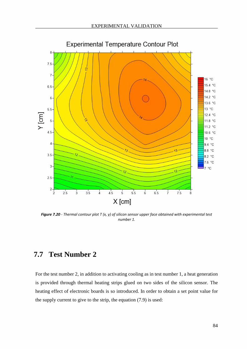
EXPERIMENTAL VALIDATION
84
Figure 7.20 - Thermal contour plot T (x, y) of silicon sensor upper face obtained with experimental test number 1.
7.7 Test Number 2
For the test number 2, in addition to activating cooling as in test number 1, a heat generation
is provided through thermal heating strips glued on two sides of the silicon sensor. The
heating effect of electronic boards is so introduced. In order to obtain a set point value for
the supply current to give to the strip, the equation (7.9) is used:
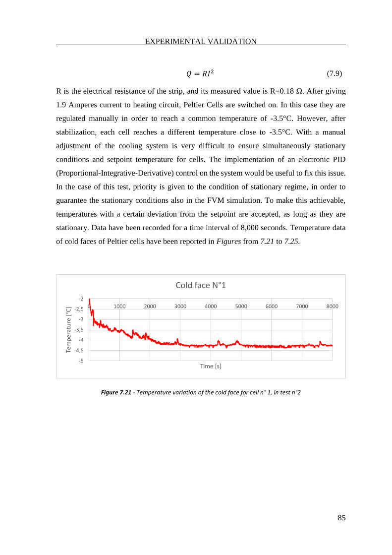
EXPERIMENTAL VALIDATION
85
𝑄 = 𝑅𝐼2 (7.9)
R is the electrical resistance of the strip, and its measured value is R=0.18 Ω. After giving
1.9 Amperes current to heating circuit, Peltier Cells are switched on. In this case they are
regulated manually in order to reach a common temperature of -3.5°C. However, after
stabilization, each cell reaches a different temperature close to -3.5°C. With a manual
adjustment of the cooling system is very difficult to ensure simultaneously stationary
conditions and setpoint temperature for cells. The implementation of an electronic PID
(Proportional-Integrative-Derivative) control on the system would be useful to fix this issue.
In the case of this test, priority is given to the condition of stationary regime, in order to
guarantee the stationary conditions also in the FVM simulation. To make this achievable,
temperatures with a certain deviation from the setpoint are accepted, as long as they are
stationary. Data have been recorded for a time interval of 8,000 seconds. Temperature data
of cold faces of Peltier cells have been reported in Figures from 7.21 to 7.25.
Figure 7.21 - Temperature variation of the cold face for cell n° 1, in test n°2
-5
-4,5
-4
-3,5
-3
-2,5
-2
0 1000 2000 3000 4000 5000 6000 7000 8000
Tem
per
atu
re [
°C]
Time [s]
Cold face N°1
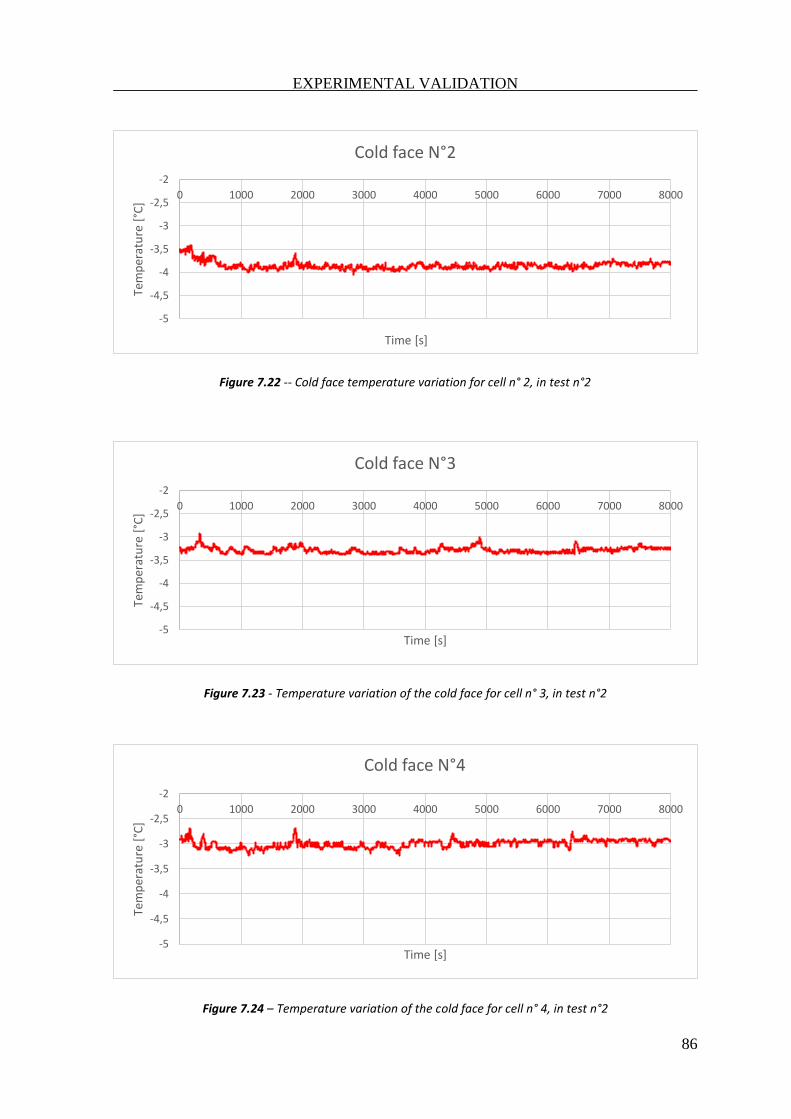
EXPERIMENTAL VALIDATION
86
Figure 7.22 -- Cold face temperature variation for cell n° 2, in test n°2
Figure 7.23 - Temperature variation of the cold face for cell n° 3, in test n°2
Figure 7.24 – Temperature variation of the cold face for cell n° 4, in test n°2
-5
-4,5
-4
-3,5
-3
-2,5
-2
0 1000 2000 3000 4000 5000 6000 7000 8000
Tem
per
atu
re [
°C]
Time [s]
Cold face N°2
-5
-4,5
-4
-3,5
-3
-2,5
-2
0 1000 2000 3000 4000 5000 6000 7000 8000
Tem
per
atu
re [
°C]
Time [s]
Cold face N°3
-5
-4,5
-4
-3,5
-3
-2,5
-2
0 1000 2000 3000 4000 5000 6000 7000 8000
Tem
per
atu
re [
°C]
Time [s]
Cold face N°4
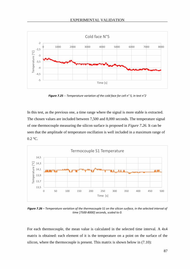
EXPERIMENTAL VALIDATION
87
Figure 7.25 -- Temperature variation of the cold face for cell n° 5, in test n°2
In this test, as the previous one, a time range where the signal is more stable is extracted.
The chosen values are included between 7,500 and 8,000 seconds. The temperature signal
of one thermocouple measuring the silicon surface is proposed in Figure 7.26. It can be
seen that the amplitude of temperature oscillation is well included in a maximum range of
0.2 °C.
Figure 7.26 – Temperature variation of the thermocouple S1 on the silicon surface, in the selected interval of time [7500-8000] seconds, scaled to 0.
For each thermocouple, the mean value is calculated in the selected time interval. A 4x4
matrix is obtained: each element of it is the temperature on a point on the surface of the
silicon, where the thermocouple is present. This matrix is shown below in (7.10):
-5
-4,5
-4
-3,5
-3
-2,5
-2
0 1000 2000 3000 4000 5000 6000 7000 8000
Tem
per
atu
re [
°C]
Time [s]
Cold face N°5
13,5
13,7
13,9
14,1
14,3
14,5
0 50 100 150 200 250 300 350 400 450 500
Tem
per
atu
re [
°C]
Time [s]
Termocouple S1 Temperature
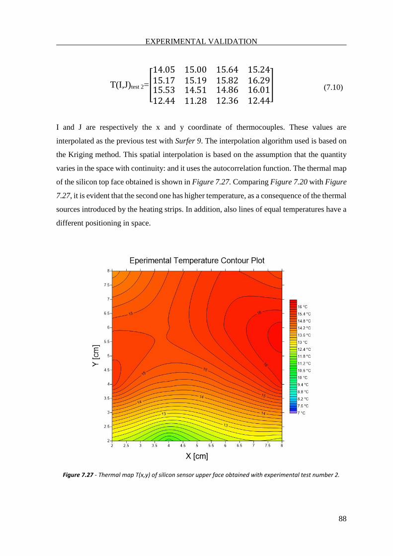
EXPERIMENTAL VALIDATION
88
T(I,J)test 2=[
14.05 15.0015.17 15.19
15.64 15.2415.82 16.29
15.53 14.5112.44 11.28
14.86 16.0112.36 12.44
]
(7.10)
I and J are respectively the x and y coordinate of thermocouples. These values are
interpolated as the previous test with Surfer 9. The interpolation algorithm used is based on
the Kriging method. This spatial interpolation is based on the assumption that the quantity
varies in the space with continuity: and it uses the autocorrelation function. The thermal map
of the silicon top face obtained is shown in Figure 7.27. Comparing Figure 7.20 with Figure
7.27, it is evident that the second one has higher temperature, as a consequence of the thermal
sources introduced by the heating strips. In addition, also lines of equal temperatures have a
different positioning in space.
Figure 7.27 - Thermal map T(x,y) of silicon sensor upper face obtained with experimental test number 2.
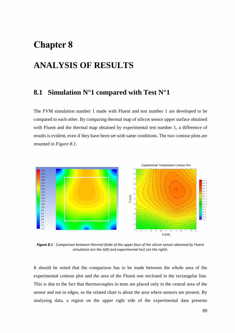
89
Chapter 8
ANALYSIS OF RESULTS
8.1 Simulation N°1 compared with Test N°1
The FVM simulation number 1 made with Fluent and test number 1 are developed to be
compared to each other. By comparing thermal map of silicon sensor upper surface obtained
with Fluent and the thermal map obtained by experimental test number 1, a difference of
results is evident, even if they have been set with same conditions. The two contour plots are
resumed in Figure 8.1.
Figure 8.1 - Comparison between thermal fields of the upper face of the silicon sensor obtained by Fluent simulation (on the left) and experimental test (on the right).
It should be noted that the comparison has to be made between the whole area of the
experimental contour plot and the area of the Fluent one enclosed in the rectangular line.
This is due to the fact that thermocouples in tests are placed only in the central area of the
sensor and not in edges, so the related chart is about the area where sensors are present. By
analysing data, a region on the upper right side of the experimental data presents
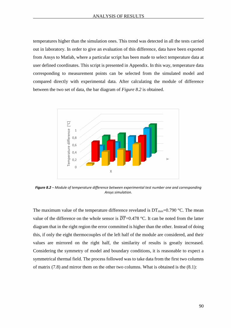
ANALYSIS OF RESULTS
90
temperatures higher than the simulation ones. This trend was detected in all the tests carried
out in laboratory. In order to give an evaluation of this difference, data have been exported
from Ansys to Matlab, where a particular script has been made to select temperature data at
user defined coordinates. This script is presented in Appendix. In this way, temperature data
corresponding to measurement points can be selected from the simulated model and
compared directly with experimental data. After calculating the module of difference
between the two set of data, the bar diagram of Figure 8.2 is obtained.
Figure 8.2 – Module of temperature difference between experimental test number one and corresponding Ansys simulation.
The maximum value of the temperature difference revelated is DTmax=0.790 °C. The mean
value of the difference on the whole sensor is 𝐷𝑇 =0.478 °C. It can be noted from the latter
diagram that in the right region the error committed is higher than the other. Instead of doing
this, if only the eight thermocouples of the left half of the module are considered, and their
values are mirrored on the right half, the similarity of results is greatly increased.
Considering the symmetry of model and boundary conditions, it is reasonable to expect a
symmetrical thermal field. The process followed was to take data from the first two columns
of matrix (7.8) and mirror them on the other two columns. What is obtained is the (8.1):
0
0,2
0,4
0,6
0,8
1
Y
Tem
per
atu
re d
iffe
ren
ce [
°C]
X

ANALYSIS OF RESULTS
91
T(I,J)mirror=[
11.39 13.4512.56 13.34
13.45 11.3913.34 12.56
12.21 12.8210.32 10.67
12.82 12.2110.67 10.32
]
(8.1)
Data have been interpolated with Kriging algorithm and the new contour plot obtained is
compared with the Fluent one, in Figure 8.3:
Figure 8.3 - Comparison between thermal fields of the upper face of the silicon sensor obtained by Fluent simulation (on the left) and mirrored values of temperatures of experimental data (on the right).
In this case the similarity is better than before. In order to evaluate the deviation of results
between the real case and the simulation model, which is proportional to the modelling error,
the punctual difference of the two thermal fields has to be calculated. Values of temperature
on the upper face of the silicon are exported from Ansys to Matlab. A specific script has been
written to find temperatures from the Ansys file at a desired (x, y, z) spatial coordinate. Whit
this algorithm, it was easy to find temperature values in the FVM in the corresponding points
where thermocouples were placed in tests. More precisely, for each coordinate (x, y, z) of
searched point, not only one value of temperature has been taken, but all the temperatures
enclosed in a square area of 2 mm. Then, for each selection, the mean value has been
calculated as reference value. This was made because the thermocouple with thermal paste,
does not provide a punctual measurement, but an average value on a very small area.
Operating in this way, sixteen values are obtained from Fluent simulations, that are directly
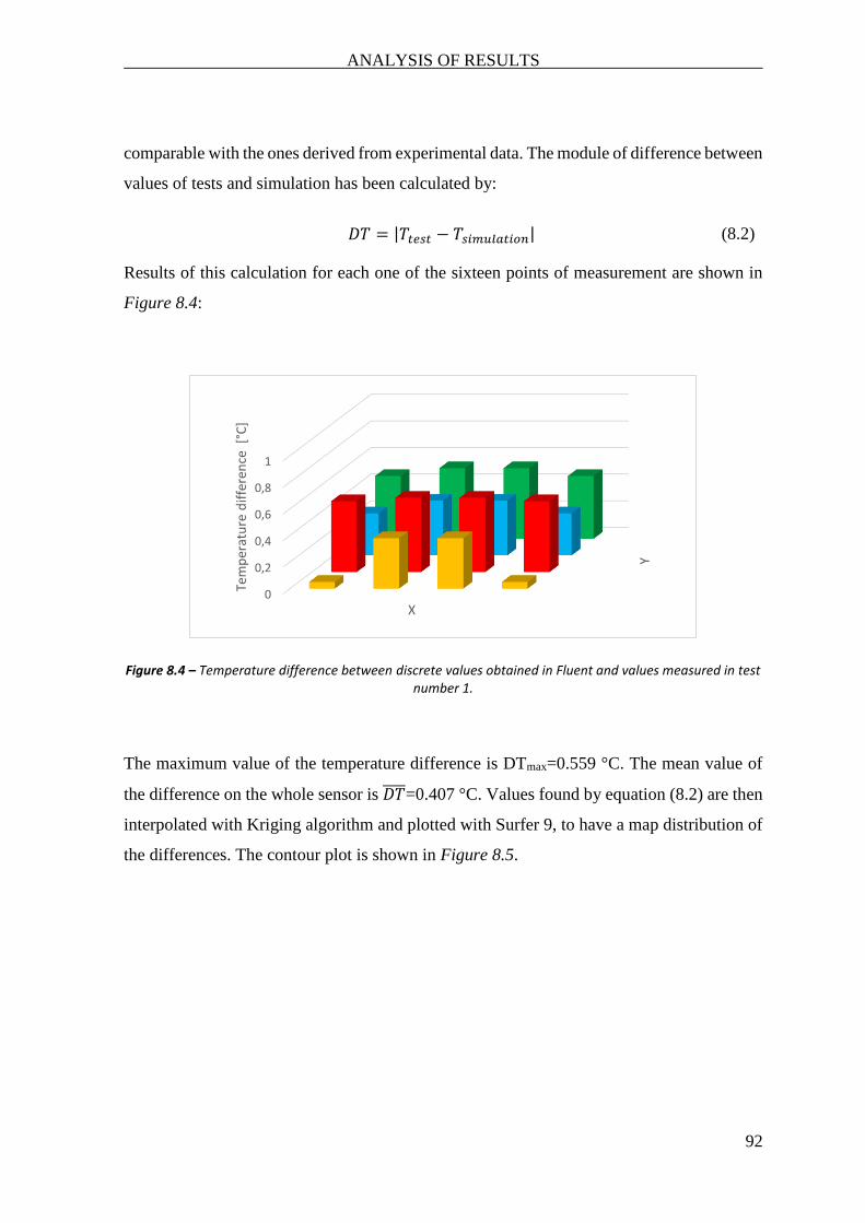
ANALYSIS OF RESULTS
92
comparable with the ones derived from experimental data. The module of difference between
values of tests and simulation has been calculated by:
𝐷𝑇 = |𝑇𝑡𝑒𝑠𝑡 − 𝑇𝑠𝑖𝑚𝑢𝑙𝑎𝑡𝑖𝑜𝑛| (8.2)
Results of this calculation for each one of the sixteen points of measurement are shown in
Figure 8.4:
Figure 8.4 – Temperature difference between discrete values obtained in Fluent and values measured in test number 1.
The maximum value of the temperature difference is DTmax=0.559 °C. The mean value of
the difference on the whole sensor is 𝐷𝑇 =0.407 °C. Values found by equation (8.2) are then
interpolated with Kriging algorithm and plotted with Surfer 9, to have a map distribution of
the differences. The contour plot is shown in Figure 8.5.
0
0,2
0,4
0,6
0,8
1
Y
Tem
per
atu
re d
iffe
ren
ce [
°C]
X
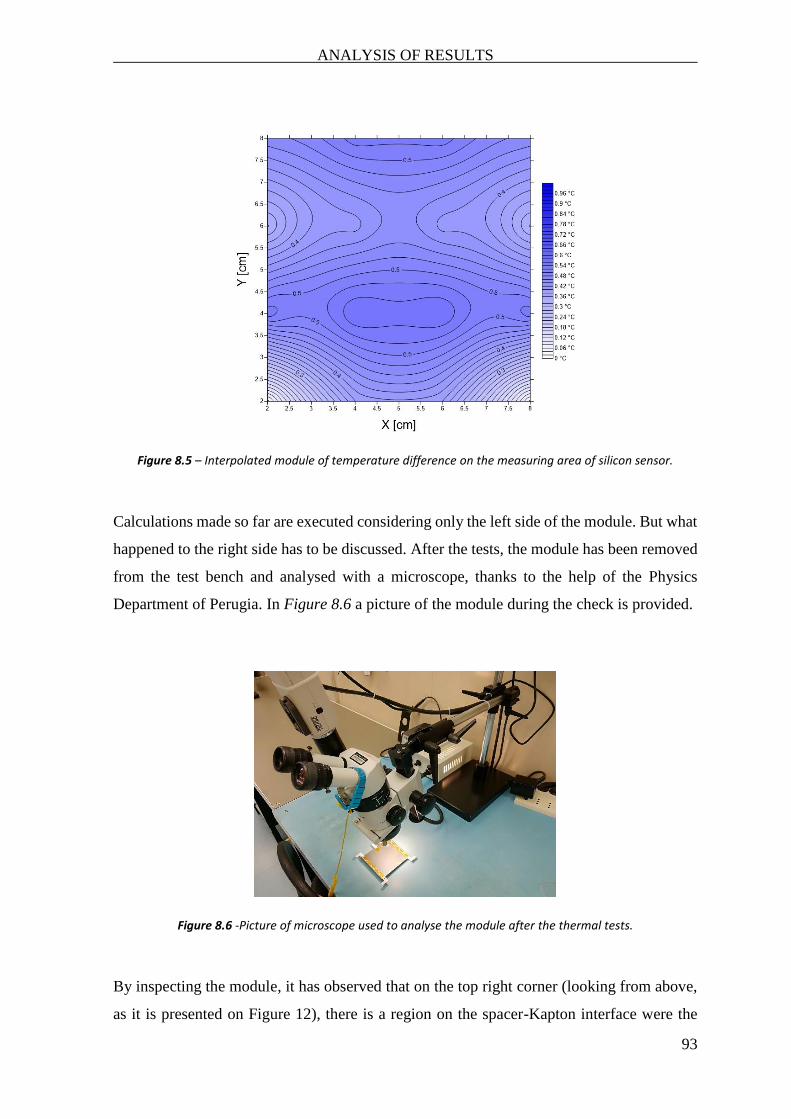
ANALYSIS OF RESULTS
93
Figure 8.5 – Interpolated module of temperature difference on the measuring area of silicon sensor.
Calculations made so far are executed considering only the left side of the module. But what
happened to the right side has to be discussed. After the tests, the module has been removed
from the test bench and analysed with a microscope, thanks to the help of the Physics
Department of Perugia. In Figure 8.6 a picture of the module during the check is provided.
Figure 8.6 -Picture of microscope used to analyse the module after the thermal tests.
By inspecting the module, it has observed that on the top right corner (looking from above,
as it is presented on Figure 12), there is a region on the spacer-Kapton interface were the
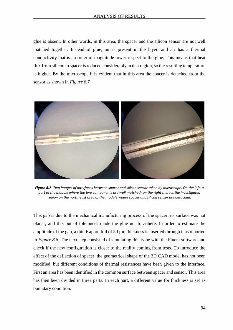
ANALYSIS OF RESULTS
94
glue is absent. In other words, in this area, the spacer and the silicon sensor are not well
matched together. Instead of glue, air is present in the layer, and air has a thermal
conductivity that is an order of magnitude lower respect to the glue. This means that heat
flux from silicon to spacer is reduced considerably in that region, so the resulting temperature
is higher. By the microscope it is evident that in this area the spacer is detached from the
sensor as shown in Figure 8.7
Figure 8.7 -Two images of interfaces between spacer and silicon sensor taken by microscope. On the left, a part of the module where the two components are well matched; on the right there is the investigated
region on the north-east area of the module where spacer and silicon sensor are detached.
This gap is due to the mechanical manufacturing process of the spacer: its surface was not
planar, and this out of tolerances made the glue not to adhere. In order to estimate the
amplitude of the gap, a thin Kapton foil of 50 µm thickness is inserted through it as reported
in Figure 8.8. The next step consisted of simulating this issue with the Fluent software and
check if the new configuration is closer to the reality coming from tests. To introduce the
effect of the deflection of spacer, the geometrical shape of the 3D CAD model has not been
modified, but different conditions of thermal resistances have been given to the interface.
First an area has been identified in the common surface between spacer and sensor. This area
has then been divided in three parts. In each part, a different value for thickness is set as
boundary condition.
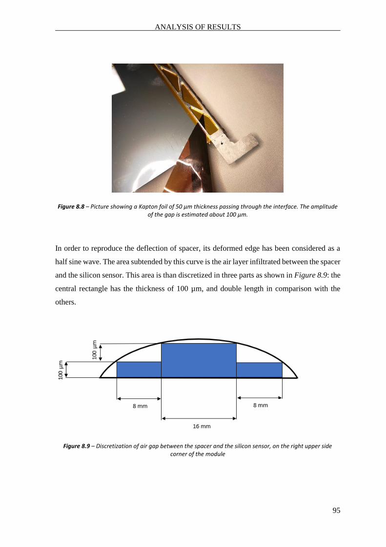
ANALYSIS OF RESULTS
95
Figure 8.8 – Picture showing a Kapton foil of 50 µm thickness passing through the interface. The amplitude of the gap is estimated about 100 µm.
In order to reproduce the deflection of spacer, its deformed edge has been considered as a
half sine wave. The area subtended by this curve is the air layer infiltrated between the spacer
and the silicon sensor. This area is than discretized in three parts as shown in Figure 8.9: the
central rectangle has the thickness of 100 µm, and double length in comparison with the
others.
Figure 8.9 – Discretization of air gap between the spacer and the silicon sensor, on the right upper side corner of the module
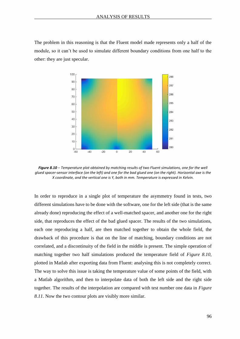
ANALYSIS OF RESULTS
96
The problem in this reasoning is that the Fluent model made represents only a half of the
module, so it can’t be used to simulate different boundary conditions from one half to the
other: they are just specular.
Figure 8.10 – Temperature plot obtained by matching results of two Fluent simulations, one for the well glued spacer-sensor interface (on the left) and one for the bad glued one (on the right). Horizontal axe is the
X coordinate, and the vertical one is Y, both in mm. Temperature is expressed in Kelvin.
In order to reproduce in a single plot of temperature the asymmetry found in tests, two
different simulations have to be done with the software, one for the left side (that is the same
already done) reproducing the effect of a well-matched spacer, and another one for the right
side, that reproduces the effect of the bad glued spacer. The results of the two simulations,
each one reproducing a half, are then matched together to obtain the whole field, the
drawback of this procedure is that on the line of matching, boundary conditions are not
correlated, and a discontinuity of the field in the middle is present. The simple operation of
matching together two half simulations produced the temperature field of Figure 8.10,
plotted in Matlab after exporting data from Fluent: analysing this is not completely correct.
The way to solve this issue is taking the temperature value of some points of the field, with
a Matlab algorithm, and then to interpolate data of both the left side and the right side
together. The results of the interpolation are compared with test number one data in Figure
8.11. Now the two contour plots are visibly more similar.

ANALYSIS OF RESULTS
97
Figure 8.11 – Comparison between test number one interpolated data (on the right) and data coming from Fluent (on the left), after the insertion of the effect of badly matched interface spacer-sensors.
In this case the difference between temperature values on corresponding points of the two
graphs are calculated. They are still proportional to the modelling error, but they also take
into account the error of interpolations and the error due to discontinuity of boundary
conditions in simulations. Module of temperature differences are reported in Figure 8.12.
Figure 8.12 - Temperature difference between discrete values obtained by matching two Fluent simulations and values measured in test number 1.
0
0,2
0,4
0,6
0,8
1
Y
Tem
per
atu
re d
iffe
ren
ce [
°C]
X

ANALYSIS OF RESULTS
98
The maximum value calculated is DTmax=0.66 °C and the average is 𝐷𝑇 =0.354 °C. It can be
noted that on the right side of the module, the temperature difference between experimental
test and simulation has lowered compared to previous cases. In the middle, a certain error is
still present, due to interpolations of two Fluent simulations. Data of module temperature
difference have been also interpolated on the measuring area, as shown in Figure 8.13.
Figure 8.13 - Interpolated module of temperature difference on the measuring area of silicon sensor, in the case of comparison between data of test number 1 ad data reconstructed by matching two Fluent
simulations.
Interpolated data of temperature difference show that in the vertical axe which splits the
area in two halves, a bigger deviation is present. This confirms that merging two fluent
simulations, it is difficult to guarantee continuity.
8.2 Simulation N°2 compared with Test N°2
The thermal map of the upper face of the silicon sensor is presented in Figure 8.14, both the
one obtained by Fluent software and the one coming from test number 2.
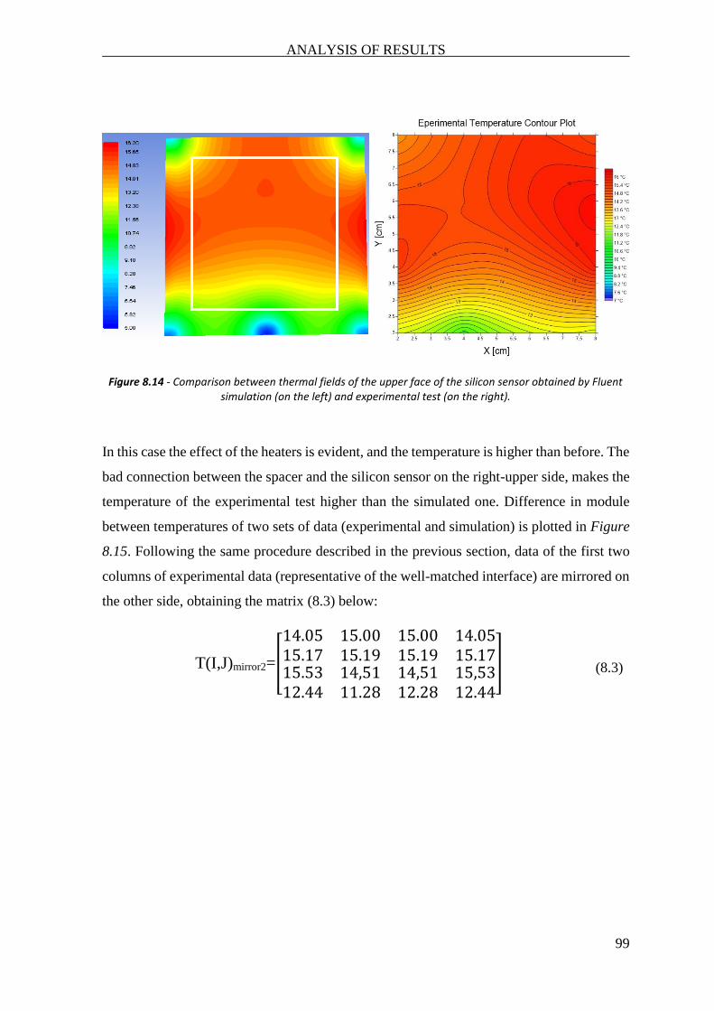
ANALYSIS OF RESULTS
99
Figure 8.14 - Comparison between thermal fields of the upper face of the silicon sensor obtained by Fluent simulation (on the left) and experimental test (on the right).
In this case the effect of the heaters is evident, and the temperature is higher than before. The
bad connection between the spacer and the silicon sensor on the right-upper side, makes the
temperature of the experimental test higher than the simulated one. Difference in module
between temperatures of two sets of data (experimental and simulation) is plotted in Figure
8.15. Following the same procedure described in the previous section, data of the first two
columns of experimental data (representative of the well-matched interface) are mirrored on
the other side, obtaining the matrix (8.3) below:
T(I,J)mirror2=[
14.05 15.0015.17 15.19
15.00 14.0515.19 15.17
15.53 14,5112.44 11.28
14,51 15,5312.28 12.44
]
(8.3)
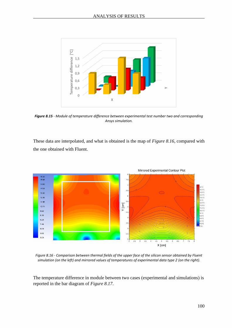
ANALYSIS OF RESULTS
100
Figure 8.15 - Module of temperature difference between experimental test number two and corresponding Ansys simulation.
These data are interpolated, and what is obtained is the map of Figure 8.16, compared with
the one obtained with Fluent.
Figure 8.16 - Comparison between thermal fields of the upper face of the silicon sensor obtained by Fluent simulation (on the left) and mirrored values of temperatures of experimental data type 2 (on the right).
The temperature difference in module between two cases (experimental and simulations) is
reported in the bar diagram of Figure 8.17.
0
0,3
0,6
0,9
1,2
1,5
Y
Tem
per
atu
re d
iffe
ren
ce [
°C]
X
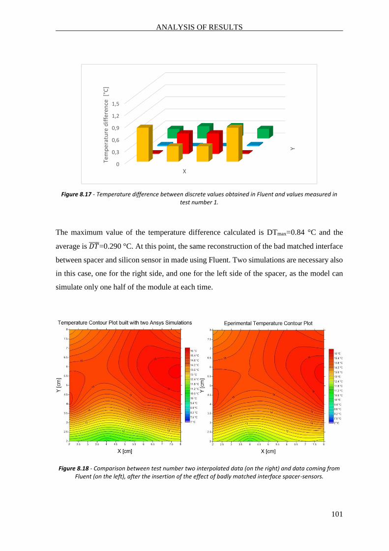
ANALYSIS OF RESULTS
101
Figure 8.17 - Temperature difference between discrete values obtained in Fluent and values measured in test number 1.
The maximum value of the temperature difference calculated is DTmax=0.84 °C and the
average is 𝐷𝑇 =0.290 °C. At this point, the same reconstruction of the bad matched interface
between spacer and silicon sensor in made using Fluent. Two simulations are necessary also
in this case, one for the right side, and one for the left side of the spacer, as the model can
simulate only one half of the module at each time.
Figure 8.18 - Comparison between test number two interpolated data (on the right) and data coming from Fluent (on the left), after the insertion of the effect of badly matched interface spacer-sensors.
0
0,3
0,6
0,9
1,2
1,5
Y
Tem
per
atu
re d
iffe
ren
ce [
°C]
X
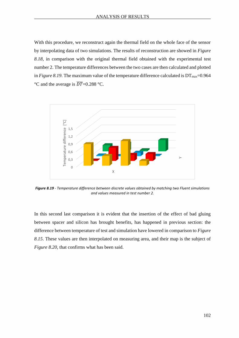
ANALYSIS OF RESULTS
102
With this procedure, we reconstruct again the thermal field on the whole face of the sensor
by interpolating data of two simulations. The results of reconstruction are showed in Figure
8.18, in comparison with the original thermal field obtained with the experimental test
number 2. The temperature differences between the two cases are then calculated and plotted
in Figure 8.19. The maximum value of the temperature difference calculated is DTmax=0.964
°C and the average is 𝐷𝑇 =0.288 °C.
Figure 8.19 - Temperature difference between discrete values obtained by matching two Fluent simulations and values measured in test number 2.
In this second last comparison it is evident that the insertion of the effect of bad gluing
between spacer and silicon has brought benefits, has happened in previous section: the
difference between temperature of test and simulation have lowered in comparison to Figure
8.15. These values are then interpolated on measuring area, and their map is the subject of
Figure 8.20, that confirms what has been said.
0
0,3
0,6
0,9
1,2
1,5
Y
Tem
per
atu
re d
iffe
ren
ce [
°C]
X
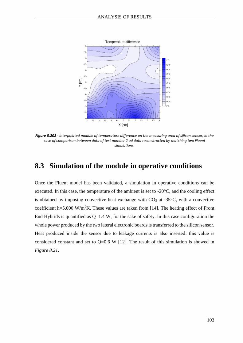
ANALYSIS OF RESULTS
103
Figure 8.202 - Interpolated module of temperature difference on the measuring area of silicon sensor, in the case of comparison between data of test number 2 ad data reconstructed by matching two Fluent
simulations.
8.3 Simulation of the module in operative conditions
Once the Fluent model has been validated, a simulation in operative conditions can be
executed. In this case, the temperature of the ambient is set to -20°C, and the cooling effect
is obtained by imposing convective heat exchange with CO2 at -35°C, with a convective
coefficient h=5,000 W/m2K. These values are taken from [14]. The heating effect of Front
End Hybrids is quantified as Q=1.4 W, for the sake of safety. In this case configuration the
whole power produced by the two lateral electronic boards is transferred to the silicon sensor.
Heat produced inside the sensor due to leakage currents is also inserted: this value is
considered constant and set to Q=0.6 W [12]. The result of this simulation is showed in
Figure 8.21.

ANALYSIS OF RESULTS
104
Figure 8.21 – Thermal contour plot of the module obtained by fluent, in the case of operative conditions of the module. Temperature is expressed in °C.
In this analysis both the top and the bottom sensors are present, as well as the air entrapped
between them and inside cavities.
Figure 8.22 – Thermal map on the silicon upper surface in operating conditions, in case of bad glued interface between sensor and spacer in the upper right side.
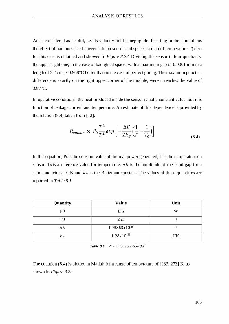
ANALYSIS OF RESULTS
105
Air is considered as a solid, i.e. its velocity field is negligible. Inserting in the simulations
the effect of bad interface between silicon sensor and spacer: a map of temperature T(x, y)
for this case is obtained and showed in Figure 8.22. Dividing the sensor in four quadrants,
the upper-right one, in the case of bad glued spacer with a maximum gap of 0.0001 mm in a
length of 3.2 cm, is 0.968°C hotter than in the case of perfect gluing. The maximum punctual
difference is exactly on the right upper corner of the module, were it reaches the value of
3.87°C.
In operative conditions, the heat produced inside the sensor is not a constant value, but it is
function of leakage current and temperature. An estimate of this dependence is provided by
the relation (8.4) taken from [12]:
𝑃𝑠𝑒𝑛𝑠𝑜𝑟 ∝ 𝑃0
𝑇2
𝑇02 𝑒𝑥𝑝 [−
∆𝐸
2𝑘𝐵(
1
𝑇−
1
𝑇0)]
(8.4)
In this equation, P0 is the constant value of thermal power generated, T is the temperature on
sensor, T0 is a reference value for temperature, ∆𝐸 is the amplitude of the band gap for a
semiconductor at 0 K and 𝑘𝐵 is the Boltzman constant. The values of these quantities are
reported in Table 8.1.
Quantity Value Unit
P0 0.6 W
T0 253 K
∆𝐸 1.93863x10⁻¹⁹ J
𝑘𝐵 1.28x10⁻²³ J/K
Table 8.1 – Values for equation 8.4
The equation (8.4) is plotted in Matlab for a range of temperature of [233, 273] K, as
shown in Figure 8.23.
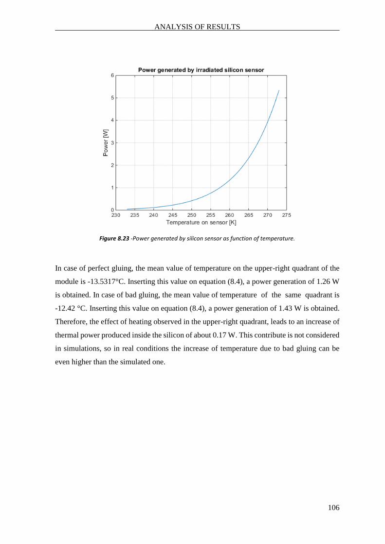
ANALYSIS OF RESULTS
106
Figure 8.23 -Power generated by silicon sensor as function of temperature.
In case of perfect gluing, the mean value of temperature on the upper-right quadrant of the
module is -13.5317°C. Inserting this value on equation (8.4), a power generation of 1.26 W
is obtained. In case of bad gluing, the mean value of temperature of the same quadrant is
-12.42 °C. Inserting this value on equation (8.4), a power generation of 1.43 W is obtained.
Therefore, the effect of heating observed in the upper-right quadrant, leads to an increase of
thermal power produced inside the silicon of about 0.17 W. This contribute is not considered
in simulations, so in real conditions the increase of temperature due to bad gluing can be
even higher than the simulated one.

107
Chapter 9
FUTURE WORKS
9.1 Developments for the FVM model.
The model proposed so far brings to good results, but it can be improved in order to reduce
the modelling error and to include more components, such as electronic boards. In various
simulations showed in this thesis, only the indirect effect of electronic heating on silicon
sensor has been modelled. Anyway, as discussed in previous sections, heat generation effect
on two sides of the module is only an approximation of reality, and it is not so easy to find
the correct value of thermal flux to insert in that point. Instead, if Front End Hybrids and
Service Hybrid are modelled, heat generation can be set exactly inside the electronic
components that are present, and the propagation of thermal fluxes will be closer to reality.
For sure, this will lead to have a higher number of elements to be simulated, and the
computational power necessary to manage them will be higher too. The same reasoning
stands for the support of the spacers: modelling CO2 cooling pipes junctions at the ends of
the spacers will bring to more confident results. Another improvement that can be done is to
simulate the whole model, and not only a half: in this way it should be possible to set
different boundary conditions from left to right in the same simulation. This development
permits to avoid the necessity of implementing two simulations, one for each half, to make
asymmetrical boundary conditions. Operating in this way, continuity of boundary conditions
in the mirroring plane are always granted and the error of interpolation is excluded. Working
on this way will also have some disadvantages, linked to the fact that the number of volume
elements will double. Furthermore, it was said that glue and Kapton have not been meshed
in the model and they have been substituted by an equivalent thermal resistance, as explained
in Section 6.3. This implies that a refinement in the treatment of the glue-Kapton-glue layers
can be done. Than, the problem of thermal runaway has to be studied more in detail, and
equation (8.4) can be implemented directly in the computational model, in order to consider
automatically this phenomenon in simulations.

FUTURE WORKS
108
Summing up, the main developments to be made on the FVM model are:
• Modelling and simulating front end hybrids, service hybrids and CO2 pipelines
junctions.
• Modelling whole module and not only a half, in order to give the possibility to set
non symmetrical boundary conditions.
• Evaluating the effect of thermal resistance, and trying to refine the coupling area
between spacers and sensors.
• Inserting the dependence of temperature on the internal heat generation of the silicon
sensor.
9.2 Developments for the test bench.
Doing tests in the bench built for experimental validation, some suggestions for
improvement have been designed. First of all, as mentioned in Section 7.6, there is the
necessity to install an electronical control (PID) for the regulation of the setpoint value for
Peltier cells. In this way, we are confident that cells stabilize exactly on the target
temperature, and not to a temperature close to it. Doing this, a new power supply system has
to be designed, in order to disengage from the five bench power supplies, which are bulky
and difficult to manage. A second update of the system is to make the pipelines of air cooling
heatsink longer, in order to eject hot air as far as possible from the fan suction. In this way
fans will not be influenced by hot air coming from other conducts. In the actual
configuration, an influence of 1°C higher than ambient temperature has been detected in fan
suction. Another implementation that can be made is creating a room around the measuring
area where the vacuum is created: fans and conducts of air cooling will pull and eject air out
from this room. In this way, the effect of convection can be excluded from measurements,
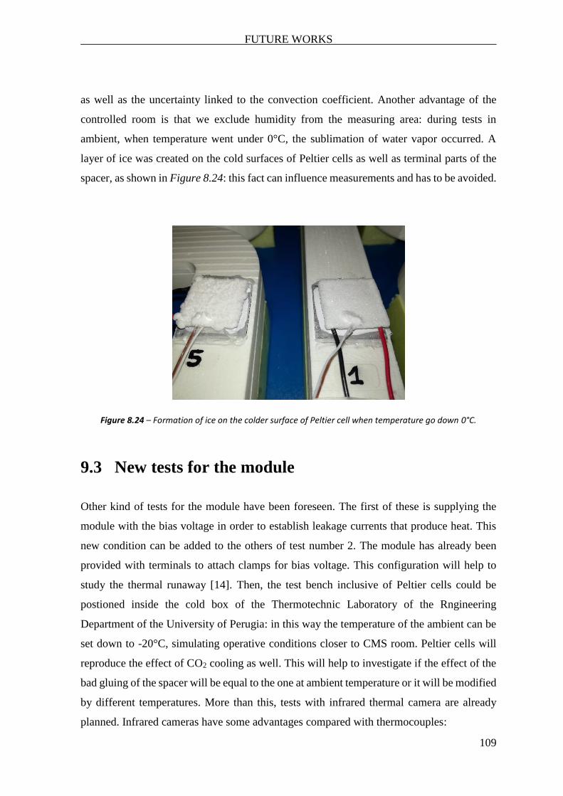
FUTURE WORKS
109
as well as the uncertainty linked to the convection coefficient. Another advantage of the
controlled room is that we exclude humidity from the measuring area: during tests in
ambient, when temperature went under 0°C, the sublimation of water vapor occurred. A
layer of ice was created on the cold surfaces of Peltier cells as well as terminal parts of the
spacer, as shown in Figure 8.24: this fact can influence measurements and has to be avoided.
Figure 8.24 – Formation of ice on the colder surface of Peltier cell when temperature go down 0°C.
9.3 New tests for the module
Other kind of tests for the module have been foreseen. The first of these is supplying the
module with the bias voltage in order to establish leakage currents that produce heat. This
new condition can be added to the others of test number 2. The module has already been
provided with terminals to attach clamps for bias voltage. This configuration will help to
study the thermal runaway [14]. Then, the test bench inclusive of Peltier cells could be
postioned inside the cold box of the Thermotechnic Laboratory of the Rngineering
Department of the University of Perugia: in this way the temperature of the ambient can be
set down to -20°C, simulating operative conditions closer to CMS room. Peltier cells will
reproduce the effect of CO2 cooling as well. This will help to investigate if the effect of the
bad gluing of the spacer will be equal to the one at ambient temperature or it will be modified
by different temperatures. More than this, tests with infrared thermal camera are already
planned. Infrared cameras have some advantages compared with thermocouples:

FUTURE WORKS
110
• They are not in contact with the object that has to be measured. They do not influence
the measurement introducing a thermal contact.
• They do not introduce electromagnetic interactions with the object as well.
Thermocouples, being in contact with bodies, can conduct electricity if a difference
of voltage is present.
• They record directly a thermal map of the object, so values have not to be
interpolated. Actually, they still furnish a discrete matrix of values, but the spatial
gap between to detected values is so small that the field can be considered continuum.
However, the main problem linked to thermal cameras is the emissivity of surfaces.
Materials of the module components are very different to each other, so emissivity can vary
a lot. More than this, the silicon surface is very reflective, so it is influenced by the external
environment. To solve this, the module can be painted with a high-emissivity paint, before
starting the tests. Some preliminary images with an infrared camera made to check the
functioning of the cooling system have been already taken and shown in Figure 8.25. In the
upper picture is shown the cooling system working without the module on the top. Peltier
cells upper faces are visibly colder than ambient. Conduits of air are hotter than ambient
from the place where heatsink of Peltier cells is inserted, as a consequence of air worming
up after flowing through fins. Motors of fans are other hot points. In the picture on the
middle, the silicon is placed in its wright position for tests. The thermal field observed on
the surface of the silicon is very similar to that of simulations. However, in this case the
stump bridge on the centre of the lower edge was not in contact with Peltier cell, and it had
not benefited from the cooling effect. This is confirmed from the fact that its colour (related
to temperature) is different from other spacers. In last picture on the bottom, is shown the 2S
module during test number 2. The heating effect of Nickel strips on the left and right edge
is visible. In this picture it is also visible the different emissivity between the adhesive tape
that fix thermocouples to sensor and the upper face of it.
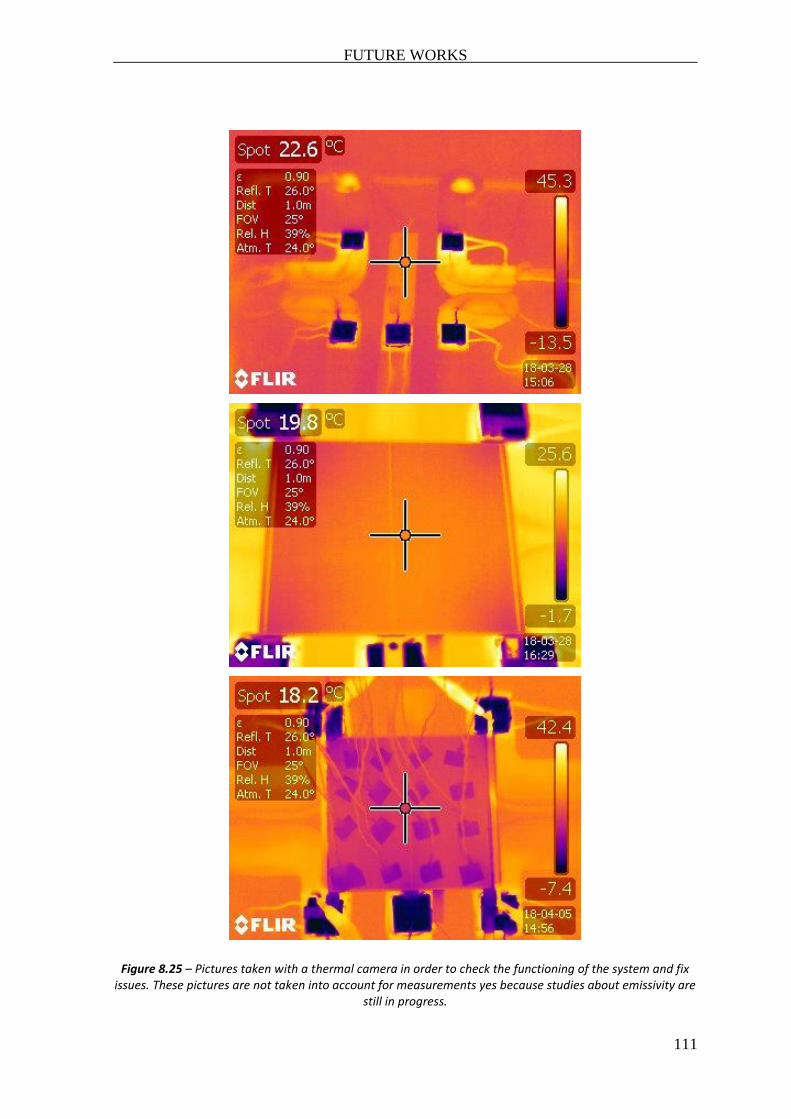
FUTURE WORKS
111
Figure 8.25 – Pictures taken with a thermal camera in order to check the functioning of the system and fix issues. These pictures are not taken into account for measurements yes because studies about emissivity are
still in progress.
112
CONCLUSIONS
The path followed to create a Finite Volume Method model for the 2 Strips module of CMS
experiment has been shown. The model has been realised with Ansys Fluent 17.1 software,
importing a 3D CAD model of the geometry given by the CMS research group. It has been
modified in order to make it suitable for the requirements of the study, and then it has been
meshed in the best way to find the better compromise between good discretization and
available calculation power. Boundary conditions have been set with reference to
experimental tests for validation, and, after that, to respect the operative conditions of the
module. The experimental validation of the model has been realised by a test system
originally ideated and built. The guidelines of this project, as well as the selection of
components have been showed. The prototype module used in tests has been built in
collaboration with the INFN (Istituto Nazionale di Fisica Nucleare) section of Perugia. The
assembly process starting from components has been presented. Two tests have been made,
each one regarding a particular set of boundary conditions: in the first one only the effect of
cooling has been analysed, while the second one has been characterised by the simultaneous
presence of cooling and heating. During tests, an unexpected result for the thermal field has
been found. This was followed by a work aimed at finding the problem, which ended
discovering an issue happened during the fabrication process. In order to understand the
nature of this issue, first a manipulation of data between simulation results and test data has
firstly been made, and, after this, the Fluent model has been modified in order to take in
account this aspect. This analysis constituted a starting point to realise some studies about
the problem found, and to see what will happen if this problem will occur during operative
conditions. After solving this issue and validating the Fluent model, the module has been
simulated in its operative conditions. A functional FVM model is now available and it can
be used for many other studies.
113
REFERENCES
[1] L. Evans and P. Bryant, “LHC Machine.” JINST 3 S08001, 2008.
[2] “Large Hadron Collider: Thirteen Ways to Change the World,” Telegraph ,
September 16, 2008, http://www.telegraph. co.uk/news/science/large-hadron-
collider/3351899/Large-Hadron-Collider-thirteen-ways-to-change-the-world.html. .
[3] “LHCb - Large Hadron Collider beauty experiment.” .
[4] THE LARGE HADRON COLLIDER - Conceptual Design.- 20 October 1995 .
[5] M. Krammer, “Design , Construction and Commissioning of the CMS Tracker at
CERN and Proposed Improvements for Detectors at the Future International Linear
Collider,” 2008.
[6] C. M. S. P. A. S. Exo- and T. C. M. S. Collaboration, “CMS Physics Analysis
Summary,” 2016.
[7] “‘ATLAS and CMS experiments present Higgs search status’. CERN. 13 December
2011. Retrieved 13 November 2016.” .
[8] “CERN Press Office (22 August 2011). ‘LHC experiments present latest results at
Mumbai conference’. press.cern. Retrieved 2016-11-13.” .
[9] “‘ATLAS releases first measurement of the W mass using LHC data’. 13 December
2016. Retrieved 27 January 2017.”
[10] P. Jandir, “Search for New Physics in All-Hadronic Events With the Compact Muon
Solenoid Experiment at the Large Hadron Collide,” UNIVERSITY OF
CALIFORNIA RIVERSIDE.
[11] “The CMS experiment/collaboration.” - 2008 .
[12] P. W. D.Abbaneo, J.Alexander, P.Azzi, E.Brodolin, A.Canepa, J.Christiansen,
S.Costa, A.Dabrowski, C.Delaere, A.Dierlamm, M.Dragicevic, R.Fruhwirth,
K.Hahn, A.Honma, K.Klein, S.Mersi, A.Mussgiller, M.Narain, A.Onnela,
G.Sguazzoni, G.Steinbrueck, J.Thom, A.Tricom, “The Phase-2 Upgrade of the CMS
114
Tracker,” 2017.
[13] A. Picerno, “Caratterizzazione di rivelatori al silicio innovativi.”- a.a.2013/2014
[14] L. Feld et al., “Thermal Measurements and FEA of the 2S Module for the CMS
Phase-2 Tracker Upgrade,” no. July, 2017.
[15] T. Technical and D. Report, “Tracker Technical Design Report,” no. April, 1998.
[16] G. Guglielmini and C. Pisoni, Elementi di trasmissione del calore, Casa editr. 1996.
[17] M. A. McAdams, Heat trasmission. 1954.
[18] “ISO 10077-2 Thermal performance of windows, doors and shutters - Calculation of
thermal transmittance,” 2012.
[19] G. Comini, G. Croce, and E. Nobile, Fondamenti di termofluidodinamica
computazionale. 2014.
[20] P. J. Roache, Verification and Validation in Computational Science and
Engineering. 1998.
[21] L. E. Schwer, Is Your Mesh Refined Enough? Estimating Discretization Error using
GCI. 2008.
[22] J. W. Slater, Examining Spatial (Grid) Convergence. 2008.
[23] M. Thakkar, A report on “Peltier (thermoelectric) cooling module.” .
[24] H. Y. Zhang, “A general approach in evaluating and optimizing thermoelectric
coolers ´ lectriques : une approche ge ´ ne ´ rale a Refroidisseurs thermoe ´ valuation
et l ’ optimisation l ’ e,” Int. J. Refrig., vol. 33, no. 6, pp. 1187–1196, 2010.
[25] S. Haidar, I. Isaac, and T. Singleton, “Thermoelectric Cooling Using Peltier Cells in
Cascade,” 1838.
[26] F. J. Disalvo, “Thermoelectric Cooling and Power Generation,” vol. 773, no.
January, 1999.
[27] H. Najafi and K. A. Woodbury, “Optimization of a cooling system based on Peltier
effect for photovoltaic cells,” Sol. Energy, vol. 91, 2013.

115
[28] Hamamatsu Photonics – www.hamamatsu.com
[29] RS Components - https://it.rs-online.com
[30] Polytec EP 601 – Polytec PTpolymere technologien - Polytec-Platz 1-7 76337
Waldbronn Germany
[31] Peltier Cell ET-071-10-13 – Adaptive
[32] Heatsink ICK S 25x25x18,5 - Fischer Elektronik
[33] Centrifugal fan – Sunon - GB1205PKV1-8AY
[34] Labview 2014 – National Instruments – www.ni.com/it-it/shop/select/labview
[35] Surfer 9 – Golden Software – www.goldensoftware.com/products/surfer
[36] Fluent 17.1 – Ansys – https://www.ansys.com
[37] SolidWorks 2013 – Dassault Systèmes – www.solidworks.it

116
APPENDIX
In this section some Matlab scripts used to take calculations for the thesis are reported.
• PROGRAM NUMBER 1
% PROGRAM TO CALCULATE GRID CONVERGENCE INDEX % IN GENERAL CASE OF r NOT COSTANT %________________________________________________________________________ %________________________________________________________________________ %Eseguire prima di questo programma 3 simulazioni in Ansys %Stabilire un parametro h indice della dimensione della mesh %Deve essere h1<h2<h3 %Il rapporto r=h(i+1)/h(i) deve essere r>1.3 %Calcolare in ciascuna delle tre simulazioni la grandezza di interesse f clc clear all close all
%Dati iniziali h1=5*10^(-6); %m h2=7.5*10^-6; %m h3=1.125*10^-5; %m
f1=317.916528; %W f2=317.82146036; %W f3=317.6528457; %W
%Algoritmo di calcolo r21=h2/h1; r32=h3/h2; if r21<1.3 disp(['Warning: il rapporto r21 è ' num2str(r21)]) disp([' ']) elseif r32<1.3
disp(['Warning: il rapporto r32 è ' num2str(r32)]) disp([' ']) end
f21=f2-f1; f32=f3-f2; s=sign(f32/f21); q=0; errore=0.00000001; %impostare errore desiderato e=100; while e>errore p=abs(log(abs(f32/f21))+q)/log(r21); qq=log((r21^p-s)/(r32^p-s)); e=qq-q; q=qq; end
e21=abs((f2-f1)/f1);

117
e32=abs((f3-f2)/f2);
%Calcolo valori di interesse f0=f1+((f1-f2)/(r21^p-1)); GCI12=1.25*e21/(r21^p-1)*100; GCI23=1.25*e32/(r32^p-1)*100; inf=f1*(1-GCI12); sup=f1*(1+GCI12); as=GCI23/(r21^p*GCI12);
disp([' GCI12= ' num2str(GCI12) ' %' ]) disp([' GCI23= ' num2str(GCI23) ' %' ]) disp([' ']) disp(['Intervallo confidenza 95% [ ' num2str(inf) ' ; ' num2str(sup) '
]'])
disp(['Soluzione estrapolata: f0=' num2str(f0)]) disp([' ']) disp(['Verifica convergenza: ' num2str(as) ' (circa 1)'])
% % Se desidero avere un certo GCI % GCIdesiderato=0.01; % GCI percentuale desiderato % % rd=(GCIdesiderato/GCI12)^(1/p); % disp([' ']) % disp([ 'Per avere GCI=' num2str(GCIdesiderato) ' devo avere r21 pari a:
' num2str(rd)])
• PROGRAM NUMBER 2
% PROGRAM TO CALCULATE PARAMETERS FOR PELTIER CELLS %STARTING FROM DATASHEET %________________________________________________________________________ %_______________________________________________________________________ clc clear all close all %________________________________________________________________________ %Dati di fabbrica Cella Imax=3.9; %A , corrente che produce il DTmax Vmax=8.8; %V , voltaggio DC massimo a DTmax DTmax=74; %K ,massima differenza di temperatura ottenibile tra le
duefacce Th0=298; %K ,temperatura parete calda a cui si realizza il DTmax Qcmax=18.7;%W ,massimo calore assorbito alla parete fredda a I=Imax e
DT=0 %________________________________________________________________________ %Parametri calcolati cella Sm=Vmax/Th0; Rm=(Th0-DTmax)*Vmax/(Th0*Imax); Km=(Th0-DTmax)*Vmax*Imax/(2*Th0*DTmax);

118
Z=(Sm^2)/(Rm*Km); %Parametri del caso operativo %LEGENDA % Ta=temperaura ambiente % Th=temperatura faccia calda cella % Tc=temperatura faccia fredda cella % Tj=temperatura "junction",temberatura fredda sul corpo da raffreddare %________________________________________________________________________ %PARAMETRI DA SCEGLIERE Tc=267; DT=46; Qc=5; Ta=296;
Th=Tc+DT; %__________________________________________________ %Algoritmo per il calcolo della corrente i=0; I=0.001; QQc=0; while QQc<Qc QQc=Sm*I*Tc-I^2*Rm/2-Km*DT; I=I+0.001; i=i+1; if I>Imax disp([' ']) disp(['ATTENZIONE!!!!! superato il limite di corrente ']) disp([' ']) disp(['Premere ctrl+c']) pause end end Qc=QQc;
%__________________________________________________ %RESISTENZA DELLA GIUNZIONE Kpt=4; % W/mK Conducibilità pasta termica ss=0.0005; % spessore pasta termica Acont=20*20*10^(-6);%mm^2,area contatto cella spacer Rjc=ss/(Kpt*Acont); %resistenza termica giunzione %________________________________________________________________________ %CALCOLI Tj=Tc+Qc*Rjc; Qh=Sm*I*Th+I^2*Rm/2-Km*DT; Qte=Sm*I*DT+Rm*I^2; COP=Qc/Qte; %Verifica:deve venire come il cop sceltro
R=(Th-Ta)/Qh; %formula semplificata Rha=((Sm*I*Rjc+Km*Rjc+1)*Qc+Km*Ta-
(Sm*I+Km)*Tj+(Rm*I^2/2))/(((Sm^2*I^2*Rjc+Sm*I)-Km)*Qc-
(Sm*I)^2*Tj+Rm*I^2*(0.5*Sm*I-Km)); %correlazione
%Rjc=((-Sm*I*Rha+Km*Rha+1)*Qc+Km*Ta+((Sm*I)^2*Rha-Sm*I-Km)*Tj+(Rm*Km*I-
0.5*Sm*Rm*I^3)*Rha+(Rm*I^2/2))/(((Sm*I)^2*Rha-Sm*I-Km)*Qc); %DDT=((Sm*I*Rha-1)*Tj+(1+Sm*I*Rjc)*Ta+Rm*I^2*(0.5*Rha-
0.5*Rjc+Sm*I*Rjc*Rha))/(Km*(Rjc+Rha)-(Sm*I*Rha-1)*(Sm*I*Rjc+1)); %Calcolo Tminima ottenibile in condizioni ideali di Rha=0

119
Tjj=Tj; RRha=Rha; while RRha>0 Tjj=Tjj-1; RRha=((Sm*I*Rjc+Km*Rjc+1)*Qc+Km*Ta-
(Sm*I+Km)*Tjj+(Rm*I^2/2))/(((Sm^2*I^2*Rjc+Sm*I)-Km)*Qc-
(Sm*I)^2*Tjj+Rm*I^2*(0.5*Sm*I-Km)); end
disp([' ']) disp(['PARAMETRI CELLA SCELTA: ' ]) disp(['C. Seebeck Sm=' num2str(Sm) ]) disp(['Res. elettrica Rm=' num2str(Rm) ]) disp(['Cond. Termica Km=' num2str(Km) ]) disp(['Z factor cella Z=' num2str(Z) ]) disp([' ']) disp(['TEMPERATURE SISTEMA: ' ]) disp(['Ta=' num2str(Ta-273) ' °C' ]) disp(['Th=' num2str(Th-273) ' °C' ]) disp(['Tc=' num2str(Tc-273) ' °C' ]) disp(['Tj=' num2str(Tj-273) ' °C' ]) disp([' ']) disp(['POTENZE: ' ]) disp(['Qc=' num2str(Qc) ' W' ]) disp(['Qh=' num2str(Qh) ' W' ]) disp(['Qelettrica=' num2str(Qte) ' W' ]) disp([' ']) disp(['Corrente assorbita: I=' num2str(I) ' A' ]) disp([' ']) disp(['Resistenza termica del dissipatore (correlazione) ' num2str(Rha)
]) disp(['Resistenza termica del dissipatore (formula semplificata) '
num2str(R) ]) disp([' ']) disp(['COP ricalcolato: COP=' num2str(COP) ]) % disp(['Con questi I, Qc, DT posso arrivare idealmente a Tjmin= '
num2str(Tjj+1-273) ' °C' ]) %________________________________________________________________________
• PROGRAM NUMBER 3
%PROGRAM TO MANAGE EXPORTATION OF RESULTS FROM ANSYS %________________________________________________________________________ %________________________________________________________________________ %Data have to be present on the Matlab Workspace clc clear all close all %Part 1 - load Ansys ASCII output file on workspace and create A matrix A(:,1)=xcoordinate;
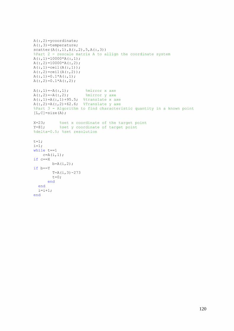
120
A(:,2)=ycoordinate; A(:,3)=temperature; scatter(A(:,1),A(:,2),5,A(:,3)) %Part 2 - rescale matrix A to allign the coordinate system A(:,1)=10000*A(:,1); A(:,2)=10000*A(:,2); A(:,1)=ceil(A(:,1)); A(:,2)=ceil(A(:,2)); A(:,1)=0.1*A(:,1); A(:,2)=0.1*A(:,2);
A(:,1)=-A(:,1); %mirror x axe A(:,2)=-A(:,2); %mirror y axe A(:,1)=A(:,1)+95.5; %translate x axe A(:,2)=A(:,2)+62.6; %Translate y axe %Part 3 - Algorithm to find characteristic quantity in a known point [L,C]=size(A);
X=23; %set x coordinate of the target point Y=81; %set y coordinate of target point %delta=0.5; %set resolution
t=1; i=1; while t==1 c=A(i,1); if c==X b=A(i,2); if b==Y T=A(i,3)-273 t=0; end end i=i+1; end

121