tesi di laurea magistrale · tesi di laurea magistrale relatore ... per esempio: “la proposizione...
TRANSCRIPT
UNIVERSITÀ DEGLI STUDI DI UDINE
DIPARTIMENTO DI MATEMATICA E INFORMATICA
CORSO DI LAUREA MAGISTRALE IN INFORMATICA
MODEL CHECKINGAND INTERVAL TEMPORAL LOGICS:CHECKING INTERVAL PROPERTIES
OF COMPUTATIONS
Tesi di Laurea Magistrale
Relatoreprof. Angelo MONTANARI
Correlatoreprof. Adriano PERON
LaureandoAlberto MOLINARI
Anno Accademico 2013/2014

UNIVERSITÀ DEGLI STUDI DI UDINE
DIPARTIMENTO DI MATEMATICA E INFORMATICA
CORSO DI LAUREA MAGISTRALE IN INFORMATICA
MODEL CHECKING AND INTERVAL TEMPORAL LOGICS:
CHECKING INTERVAL PROPERTIES OF COMPUTATIONS
MODEL CHECKING E LOGICHE TEMPORALI A INTERVALLI:VERIFICARE PROPRIETÀ INTERVALLARI DELLE COMPUTAZIONI
Tesi di Laurea Magistrale
Relatoreprof. Angelo MONTANARI
Correlatoreprof. Adriano PERON
LaureandoAlberto MOLINARI
Anno Accademico 2013/2014

Abstract
Model checking is an alternative to simulation and testing, two classic techniquesof software engineering for software validation, which consists in expressing someproperties of a finite-state transition system in formulas of a temporal logic and thenverifying them over a model of the system itself (usually a finite Kripke structure)through exhaustive enumeration of all the reachable states. This technique is fullyautomatic and every time the design violates a desired property, a counterexample isproduced, which illustrates a behavior that falsifies the property.
All model checking techniques, such as partial order reduction, symbolic andbounded model checking, were developed some years ago bearing in mind the well-known “point-based” temporal logics LTL and CTL. However, while the expressivenessof such logics is beyond doubt, there are some properties we may want to check thatare inherently “interval-based” and thus can not be expressed by point-based tempo-ral logics, e.g., “p has to hold in at least an average number of system states in a givencomputation sector”. Here interval temporal logics (ITLs) come into play, providingan alternative setting for reasoning about time. Such logics deal with intervals, in-stead of points, as their primitive entities; this choice gives them the ability to expresstemporal properties, such as actions with duration, accomplishments, and temporalaggregations, which cannot be dealt with in standard (point-based) logics.
A prominent position among ITLs is occupied by Halpern and Shoham’s modallogic of time intervals (HS, for short). HS features one modality for each of the 13possible ordering relations between pairs of intervals, apart from the equality relation.
Here, we focus our attention on the model checking problem for HS, for which alittle work has been done, if compared to model checking for point-based temporallogics.
The idea is to evaluate HS formulas on finite Kripke structures, making it possibleto check the correctness of the behavior of systems with respect to meaningful intervalproperties. To this end, we interpret each finite path (i.e., a track) in a Kripke structureas an interval, and we define its labeling on the basis of the labeling of the states thatcompose it.
Formally, we will show that finite Kripke structures can be suitably mapped intointerval-based structures, called abstract interval models, over which HS formulascan be interpreted. Such models have in general an infinite domain, because finiteKripke structures may have loops and thus infinitely many tracks. In order to devisea model checking procedure for HS over finite Kripke structures, we prove a smallmodel theorem showing that, given an HS formula ψ and a finite Kripke structureK , there exists a finite interval model which is equivalent to the one induced byK with respect to the satisfiability of ψ. In this way we can prove that the modelchecking problem for HS interpreted over finite Kripke structures is decidable (with anon-elementary upper bound); in addition we show it is EXPSPACE-hard if a succinctencoding of HS formulas is exploited.
Then we restrict our attention to the fragment HS[A, A,B ,B ,E ], consisting of HSformulas with modalities A, A, B , B and E only, and we prove that its model checkingis in EXPSPACE by exploiting track representatives, which are the only bounded-lengthtracks we need to take into consideration when checking an HS[A, A,B ,B ,E ] formulaover a Kripke structure.
Finally, we consider the fragments HS[A, A,B ,E ] and ∀HS[A, A,B ,E ], whosemodel checking problems are PSPACE-complete and coNP-complete, respectively.

Sommario
Il model checking si propone come un’alternativa alla simulazione e al testing,due tecniche classiche dell’ingegneria del software per la validazione del software;esso consiste nell’esprimere alcune proprietà di un sistema di transizione a statifiniti mediante formule di una logica temporale e, successivamente, nel verificarlesu un modello del sistema stesso (di solito una struttura di Kripke finita), tramitel’enumerazione completa di tutti gli stati raggiungibili. Questa tecnica è totalmenteautomatica ed ogni volta che viene violata una proprietà desiderata, viene fornito uncontroesempio che illustra un comportamento che falsifica tale proprietà.
Tutte le tecniche del model checking, come la partial order reduction, il symboliced il bounded model checking, sono state sviluppate prendendo in considerazionele logiche temporali LTL e CTL, che sono basate su punti. Tuttavia, nonostantel’indubbia espressività di tali logiche, esistono alcune proprietà che potremmo volerverificare, che hanno inerentemente una semantica intervallare e quindi non possonoessere espresse da logiche puntuali, per esempio: “la proposizione p deve valere inalmeno un dato numero medio di stati del sistema, in un settore di computazionefissato”. Le logiche temporali a intervalli entrano in gioco in questi casi: esse adottanogli intervalli, invece dei punti, come loro entità primitive. Tale caratteristica dà lorol’abilità di esprimere proprietà intervallari, come azioni con durata, conseguimentidi obiettivi e aggregazioni temporali, che non possono essere trattate nelle logiche(puntuali) standard.
Una posizione prominente fra le logiche a intervalli è occupata dalla logica mo-dale degli intervalli temporali di Halpern e Shoham (HS in breve): essa possiedeuna modalità per ognuna delle 13 possibili relazioni di ordinamento fra coppie diintervalli, eccetto l’uguaglianza. In questa tesi viene considerato il problema delmodel checking per HS, il quale ha ricevuto ben poca attenzione in letteratura inconfronto al model checking per logiche temporali puntuali.
L’idea è quella di valutare formule di HS su strutture di Kripke finite, per riuscire averificare la correttezza del comportamento di un sistema rispetto a proprietà inter-vallari. A questo scopo interpretiamo ogni percorso finito di una struttura di Kripke,detto anche traccia, come un intervallo e definiamo l’etichettatura di quest’ultimosulla base dell’etichettatura degli stati che lo costituiscono. Mostreremo infatti che lestrutture di Kripke possono essere mappate in certe strutture intervallari, chiama-te abstract interval models, sulle quali le formule di HS vengono interpretate; essehanno in generale un dominio infinito, perché le strutture di Kripke possono averecicli e quindi infinite tracce. Al fine di sviluppare una procedura di model checkingper HS su strutture di Kripke finite, proviamo uno small model theorem che dimostrache data una formula di HS ψ e una struttura di Kripke finita K , esiste un intervalmodel finito che è equivalente a quello indotto da K rispetto alla soddisfacibilità diψ. In questo modo riusciamo a dimostrare che il problema del model checking perHS interpretato su strutture di Kripke finite è decidibile (con un upper bound nonelementare); in aggiunta esso è EXPSPACE-hard, se si sfrutta una codifica succintadelle formule di HS.
Poi passiamo a considerare il frammento HS[A, A,B ,B ,E ], costituito dalle formu-le di HS con le sole modalità A, A, B , B , E , e dimostriamo che per tale frammento ilmodel checking è in EXPSPACE; sfruttiamo a questo scopo i rappresentanti di tracce:essi sono le sole tracce di lunghezza limitata che è necessario prendere in considera-zione quando si deve verificare una formula di HS[A, A,B ,B ,E ] su una struttura diKripke.
Infine analizziamo i frammenti HS[A, A,B ,E ] e ∀HS[A, A,B ,E ]: il problema delmodel checking per il primo è PSPACE-completo, coNP-completo per il secondo.


Ringrazio i professori Angelo Montanari e Adriano Peron per ilsupporto che non mi hanno mai fatto mancare in questi sei mesidi lavoro.
Desidero ringraziare in particolare il prof. Montanari per avermiaiutato in un momento di difficoltà.

Contents
1 Introduction 11.1 An overview of model checking and interval temporal logics . . . . . . 11.2 Organization of the thesis . . . . . . . . . . . . . . . . . . . . . . . . . . . 41.3 Related work . . . . . . . . . . . . . . . . . . . . . . . . . . . . . . . . . . . 5
2 HS, Abstract Interval Models and Descriptors 72.1 The interval temporal logic HS . . . . . . . . . . . . . . . . . . . . . . . . 72.2 Kripke structures and abstract interval models . . . . . . . . . . . . . . . 92.3 The fundamental notion of BEk -descriptor . . . . . . . . . . . . . . . . . 13
3 Decidability of model checking for HS and EXPSPACE-hardness 233.1 The decidability proof . . . . . . . . . . . . . . . . . . . . . . . . . . . . . 233.2 k-equivalence and corresponding BEk -descriptors . . . . . . . . . . . . 263.3 EXPSPACE-hardness of HS model checking . . . . . . . . . . . . . . . . . 31
4 A model checking algorithm based on track representatives 394.1 Descriptor element indistinguishability . . . . . . . . . . . . . . . . . . . 404.2 Track representatives . . . . . . . . . . . . . . . . . . . . . . . . . . . . . . 464.3 The model checking algorithm . . . . . . . . . . . . . . . . . . . . . . . . 534.4 NEXP-hardness of model checking for HS[A, A,B ,B ,E ] . . . . . . . . . . 55
5 Some well-behaved fragments of HS 575.1 The fragments ∀HS[A, A,B ,E ], HS[A, A], and HS[Prop] . . . . . . . . . 595.2 The fragment HS[A, A,B ,E ] . . . . . . . . . . . . . . . . . . . . . . . . . . 64
6 Conclusions 67
A Appendix 69A.1 Proofs of Chapter 3 . . . . . . . . . . . . . . . . . . . . . . . . . . . . . . . 69
A.1.1 Proof of Lemma 3.9 . . . . . . . . . . . . . . . . . . . . . . . . . . . 69A.1.2 Proof of Lemma 3.10 . . . . . . . . . . . . . . . . . . . . . . . . . . 70
A.2 Proofs of Chapter 4 . . . . . . . . . . . . . . . . . . . . . . . . . . . . . . . 71A.2.1 Proof of Lemma 4.1 . . . . . . . . . . . . . . . . . . . . . . . . . . . 71

xii ¦
A.2.2 Proof of Theorem 4.20 . . . . . . . . . . . . . . . . . . . . . . . . . 72A.2.3 Proof of Theorem 4.24 . . . . . . . . . . . . . . . . . . . . . . . . . 74A.2.4 Proof of Lemma 4.25 . . . . . . . . . . . . . . . . . . . . . . . . . . 74
A.3 Proofs of Chapter 5 . . . . . . . . . . . . . . . . . . . . . . . . . . . . . . . 75A.3.1 Proof of Theorem 5.4 . . . . . . . . . . . . . . . . . . . . . . . . . . 75
Bibliography 81
1Introduction
Contents1.1 An overview of model checking and interval temporal logics . . . 11.2 Organization of the thesis . . . . . . . . . . . . . . . . . . . . . . . . 41.3 Related work . . . . . . . . . . . . . . . . . . . . . . . . . . . . . . . . 5
1.1 An overview of model checking and intervaltemporal logics
IT systems are becoming more and more pervasive in our lives; software is normallyresponsible for their operation, even in the case of hard-realtime and fault-intolerantsystems, such as telephone networks, traffic control systems, medical instruments,e-commerce, . . . where reliability is an essential requirement. However, the typicaltechniques of software engineering for software validation, that is, simulation andtesting, have become outdated and are clearly not sufficient alone in several modernscenarios; their effectiveness decreases dramatically as the complexity of designgrows, they do not always guarantee high quality results and often discover errorsand unpredictable behaviors in software at late stages of development (or even whenit has already been deployed). Moreover, such traditional methods are not effectiveat discovering the more subtle and hidden bugs.
Formal verification is an alternative to simulation and testing, which explores allthe possible states and scenarios of a system, in order to prove that it features some de-sired properties such as correctness, deadlock freedom, data integrity, liveness, safety,fairness, responsiveness, interference freedom and so on. The two most famousapproaches to formal verification are axiomatic reasoning and model checking.
Axiomatic reasoning involves specifying the desired properties of a system bymeans of formulas; then a proof system, consisting of axioms and rules, allows toformally prove that the system meets the expected behavior. An example is Hoare’stuple-based proof system. However, this method has several limitations, being the
2 ¦ Chapter 1. Introduction
most significant: the proof rules are designed only for a posteriori verification ofexisting software, not for its systematic development; moreover such a technique isvery time consuming, cumbersome, and can be performed only by experts: as a con-sequence, it is mostly employed for (parts of) critical systems or security protocols.
In model checking [CE81, CGP02, QS81, VW86] some properties of a finite-statetransition system are expressed in a temporal logic and then verified over a model ofthe system itself (usually a Kripke structure) through exhaustive (implicit or explicit)enumeration of all the reachable states. This technique is fully automatic and everytime the design violates a desired property, a counterexample is produced, whichillustrates a behavior that falsifies the property. Model checking techniques allow toanalyze even partial specifications, in such a way that it is not necessary to completelyspecify the system before information can be obtained regarding its correctness.
The first attempt in this direction goes back to 1977, when the use of the lineartemporal logic LTL in program verification was proposed by Pnueli [Pnu77]. LTLallows one to reason about changes in the truth value of formulas in a Kripke structureover a linearly-ordered temporal domain, where each moment in time has a uniquepossible future. More precisely, one has to consider all possible paths in a Kripkestructure and to analyze, for each of them, how proposition letters, labeling the states,change from one state to the next one along the path.
The model checking problem for LTL turns out to be PSPACE-complete [CGP02,Pnu81]. This logic has been also investigated with respect to the satisfiability problem,useful for example in planning, which is, again, PSPACE-complete.
Four years later, in 1981, Clarke and Emerson invented the branching time logicCTL [CE81], whose model of time is a tree, i.e., the future is not determined, asthere are different paths in the future, any one of which may be realized. The modelchecking problem for CTL is in P, while its satisfiability is EXP-complete. However,these two logics are somewhat complementary, as there are properties expressible inonly one of CTL and LTL.
Software is extremely flexible and, as time goes by, it tends to get more and morecomplex: therefore model checking techniques have to cope with the problem ofstate explosion, which becomes particularly serious when the system being verified isvery complex or many components are working in parallel. Symbolic model checking[BCM+90, CM90, McM93] allows an exhaustive implicit enumeration of a huge quan-tity of states (even more than 10120): ordered binary decision diagrams (OBDDs),particular data structures for representing boolean functions, are exploited in orderto get concise representations of transition systems and to efficiently manipulatethem. A very successful model checker was developed based on OBDDs: SMV.
Partial order reduction [Pel93] tries to reduce the size of the state space by makingcomputations that differ only in the ordering of independently executed actions col-lapse, as they are indistinguishable by the specification (i.e., they can be consideredequivalent) and only one for each group needs to be tested. The model checker SPINmakes use of the partial order reduction technique.
Another, by now traditional model checking method is bounded model check-ing [BCC+03]: proposed in [BCC+99], its basic idea is searching a counterexamplein computations whose length is bounded by a fixed integer k. So, either a bug isfound, or one can increase k until the problem becomes intractable, or the so-calledcompleteness threshold is reached (i.e., for high enough values of k, this technique isguaranteed to find any existing counterexample). In bounded model checking boththe specifications of the system and properties to be checked have to be translatedinto a propositional formula. In this way, it is possible to employ SAT-solvers in model
1.1. An overview of model checking and interval temporal logics ¦ 3
checking, which are less sensitive to the state explosion problem than OBDD-basedsolvers. However this method is in general incomplete if the bound is not high enough,hence it used as a complementary technique to OBDD-based symbolic model check-ing: the former is usually exploited for falsification, i.e., finding counterexamples andbugs, while the latter for verification.
All of these techniques were developed some years ago, bearing in mind the“point-based” temporal logics LTL and CTL. However, while the expressiveness of suchlogics is beyond doubt, there are some properties we might want to check that areinherently “interval-based” and thus can not be expressed by point-based temporallogics, e.g., “the proposition p has to hold in at least an average number of systemstates in a given computation sector”. Here interval temporal logics (ITLs) come intoplay, providing an alternative setting for reasoning about time [HS91, Ven90, Ven91].Such logics deal with intervals, instead of points, as their primitive entities; thischoice gives them the ability to express temporal properties, such as actions withduration, accomplishments, and temporal aggregations, which can not be dealt within standard (point-based) logics.
ITLs have been applied in a variety of computer science fields, including artificialintelligence (reasoning about action and change, qualitative reasoning, planning[BT03], configuration and multi-agent systems [GT99, LR06] and computationallinguistics [Pra05]), theoretical computer science (formal verification [CH04, Mos83]),and databases (temporal and spatio-temporal databases [GMS04]).
A prominent position among ITLs is occupied by Halpern and Shoham’s modallogic of time intervals (HS, for short) [HS91]. HS features one modality for each ofthe 13 possible ordering relations between pairs of intervals (the so-called Allen’srelations [All83]), apart from the equality relation. As an example, the condition: “thecurrent interval meets an interval over which p holds” can be expressed in HS by theformula ⟨A⟩p, where ⟨A⟩ is the (existential) HS modality for Allen’s relation meet.
In [HS91], it was shown that the satisfiability problem for HS interpreted overall relevant classes of linear orders is undecidable. For example, it is undecidableoverN, Z,Q and R, as well as over the classes of all dense, discrete and finite linearorders. Since then, a lot of work has been done on the satisfiability problem for HSfragments [DGMS11], which showed that undecidability rules over them [BDG+14,Lod00, MM14]. As an example, the fragment HS[B ,E ] (i.e., formulas of HS with Band E modalities only) is undecidable, again, over the class of all linear orders, overall dense linear orders, discrete linear orders and finite linear orders.
However, meaningful exceptions exist, including the interval logic of temporalneighbourhood HS[A, A] and the temporal logic of sub-intervals HS[D] [BGMS10,BGMS09, BMSS11b, MPS10, MMS12, MS12, BMSS11a]. In particular, the former isdecidable over the class of all linear orders, and over all finite, discrete and denselinear orders (also over N, Z,Q and R); as for the latter, the situation is more involved:HS[D] is decidable over all dense linear orders (e.g., Q), undecidable over discretelinear orders and finite linear orders [MM14], and it is not known whether it is decid-able or not in the case of all linear orders. Some other fragments, such as HS[B ,B ]and HS[E ,E ], have actually a point-based semantics: one of the endpoints of everyinterval related to the current one can “move”, but the other remains fixed; as a con-sequence they can be polynomially translated to a basic point-based temporal logic;it follows that they are decidable over the class of all linear orders and, in particular,NP-complete. On the other hand, another fragment, HS[A, A,B ,B ], is decidable overfinite linear orders, Q, as well as over the class of all linear orders, but undecidableover Dedekind-complete linear orders (in particular,N and R) [MPS14].
4 ¦ Chapter 1. Introduction
Here we focus our attention on the model checking problem for HS, for which alittle work has been done, if compared to satisfiability of HS and especially to modelchecking of point-based temporal logics. The idea is to evaluate HS formulas onfinite Kripke structures, making it possible to check the correctness of the behaviorof systems with respect to meaningful interval properties. To this end, we interpreteach finite path (i.e., a track) in a Kripke structure as an interval, and we define itslabeling on the basis of the labeling of the states that compose it, according to thehomogeneity assumption [Roe80] (i.e., a proposition letter p holds on an interval I ifand only if p holds on all the subintervals of I ).
The next section provides an overview of how we tackle the problem of HS modelchecking by describing the contents of the following chapters.
1.2 Organization of the thesis
In Chapter 2, after giving syntax and semantics of HS (Section 2.1), we show thatfinite Kripke structures can be suitably mapped into interval-based structures, calledabstract interval models, over which HS formulas can be interpreted (Section 2.2).Such models have, in general, an infinite domain, as finite Kripke structures may haveloops and thus an infinite number of tracks. Moreover we introduce track descriptors,tree-like structures which give information about (possibly infinite) sets of tracks andallow us to define a finite-index equivalence relation over tracks (Section 2.3). Thereference for this chapter is [MMPP14].
In Chapter 3, in order to show that the model checking problem for HS over finiteKripke structures is decidable, we prove a small model theorem (Section 3.1), whichheavily rests on track descriptors, demonstrating that, given an HS formula ψ and afinite Kripke structure K , there exists a finite interval model which is equivalent tothe one induced by K with respect to the satisfiability ofψ (here we follow [MMPP14]again). Then, in Section 3.2, we introduce the novel notion of correspondence betweendescriptors, which allows us to precisely capture the relation of equivalence betweentracks with respect to satisfiability of HS formulas. Finally, in Section 3.3, we show thatthe model checking problem for HS over finite Kripke structures is EXPSPACE-hard,if a succinct encoding of formulas is used.
In Chapter 4, in an attempt to lower the complexity of model checking, we analyzethe fragment HS[A, A,B ,B ,E ] (i.e., formulas of HS with A, A, B , B and E modalitiesonly). In Section 4.1 we present the notions of cluster and descriptor element indis-tinguishability, which allow to determine when two tracks are associated with thesame descriptor, without directly building it—an operation which is very expensive interms of complexity, due to the size of such structures. In Section 4.2 track represen-tatives are introduced: they are tracks of bounded length, each of which is consideredin place of all other tracks associated with its descriptor. Due to their finite length,their quantity is finite, and we can exploit them to provide an EXPSPACE modelchecking algorithm for HS[A, A,B ,B ,E ]. Finally, in Section 4.4, by rephrasing theproof of Section 3.3, we prove that the model checking problem for HS[A, A,B ,B ,E ]is NEXP-hard if a suitable succinct encoding of formulas is exploited.
In the last chapter (Chapter 5) we analyze some more fragments of HS of lowercomplexity, which can still express meaningful properties of transition systems. InSection 5.1 we provide a model checking algorithm for a fragment which turns outto be coNP-complete, ∀HS[A, A,B ,E ] (i.e., formulas of HS[A, A,B ,E ] where onlyuniversal modalities and conjunctions are allowed) and in Section 5.2 we study the
1.3. Related work ¦ 5
PSPACE-complete fragment HS[A, A,B ,E ].A final overview of the results reached in this thesis is given in Chapter 6, together
with the conclusions.Finally, the Appendix A contains some proofs which are not directly presented
with the corresponding theorems/lemmas, because particularly long and technical.
1.3 Related workAs already mentioned, the model checking problem for interval temporal logics hasnot been extensively studied in literature. Indeed, to our knowledge the only threepapers that deal with HS model checking are [MMPP14, LM13, LM14].
In [MMPP14], Montanari et al. give a first characterization of the model checkingproblem for full HS, interpreted over finite Kripke structures (under the homogeneityassumption). In that paper, the authors provide the basic elements of the generalpicture, namely, the interpretation of HS formulas over abstract interval models,the mapping of finite Kripke structures into abstract interval models, the notion oftrack descriptor, and the small model theorem proving the decidability of the modelchecking problem for full HS against finite Kripke structures. We will present andextend these results in chapters 2 and 3.
In [LM13, LM14], Lomuscio and Michaliszyn address the model checking prob-lem for some fragments of HS extended with epistemic modalities. Their semanticassumptions differ from those made in [MMPP14], making it difficult to comparethe outcomes of the two research directions. In both cases, formulas of intervaltemporal logic are evaluated over tracks obtained from the unravelling of a finiteKripke structure. However, in [MMPP14] the authors state that a proposition letterholds over a track if and only if it holds over all its states (homogeneity principle),while in [LM13, LM14] truth of proposition letters is defined over pairs of states (theendpoints of tracks).
In [LM13], the authors focus their attention on the fragment HS[B ,E ,D] (sincemodality D is easily definable in terms of modalities B and E , HS[B ,E ,D] is actuallyas expressive as HS[B ,E ]), extended with epistemic modalities. They consider arestricted form of model checking, which verifies the given specification against a sin-gle (finite) initial computation interval. Their goal is indeed to reason about a givencomputation of a multi-agent system, rather than on all its admissible computations.The authors prove that the considered model checking problem is PSPACE-complete.Moreover, they show that the same problem restricted to the purely temporal frag-ment HS[B ,E ,D], that is, the one obtained by removing epistemic modalities, is in P.These results do not come as a surprise as they trade expressiveness for efficiency:modalities B and E allow one to access only sub-intervals of the initial one, whosenumber is quadratic in the length (number of states) of the initial interval.
In [LM14], they show that the picture drastically changes with other fragmentsof HS, that allow one to access infinitely many tracks/intervals. In particular, theyprove that the model checking problem for the fragment HS[A,B ,L] (since modalityL is easily definable in terms of modality A, HS[A,B ,L] is actually as expressive asHS[A,B ]), extended with epistemic modalities, is decidable with a non-elementaryupper bound. Notice that, thanks to modalities A and B , formulas of this logic canpossibly refer to infinitely many (future) tracks/intervals.

2HS, Abstract Interval Models
and Descriptors
Contents2.1 The interval temporal logic HS . . . . . . . . . . . . . . . . . . . . . 72.2 Kripke structures and abstract interval models . . . . . . . . . . . 92.3 The fundamental notion of BEk -descriptor . . . . . . . . . . . . . 13
In this chapter, we first give syntax and semantics of Halpern and Shoham’sinterval temporal logic HS with respect to abstract interval models. Then, we providea suitable mapping from Kripke structures to abstract interval models that allowsus to interpret HS formulas over Kripke structures and then to define the notion ofinterval-based model checking.
Finally we introduce the notion of track descriptor, which allows to prove that,considered a Kripke structure K and an HS formula ψ, there exists a finite abstractinterval model which is equivalent to the possibly infinite model corresponding to Kwith respect to satisfiability of ψ.
2.1 The interval temporal logic HSAn interval algebra to reason about intervals and their relative order was first pro-posed by Allen in [All83]; then, a systematic logical study of interval representationand reasoning was done by Halpern and Shoham, who introduced the interval tem-poral logic HS [HS91]; such a logic features one modality for each of the possiblebinary ordering relations between a pair of intervals (the so-called “Allen’s relations”),except for the equality.
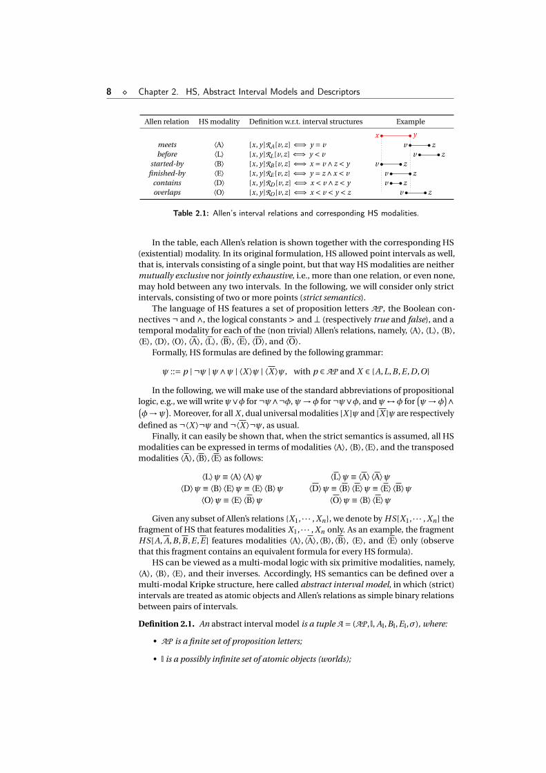
Table 2.1 depicts 6 of the 13 Allen’s relations; the other 7 are the 6 inverse relations(given a generic binary relation R , the inverse relation R holds between two elements,bR a, if and only if aR b), and the equality.
8 ¦ Chapter 2. HS, Abstract Interval Models and Descriptors
Allen relation HS modality Definition w.r.t. interval structures Example
x yv z
v zv z
v zv z
v z
meets ⟨A⟩ [x, y]RA[v, z] ⇐⇒ y = vbefore ⟨L⟩ [x, y]RL[v, z] ⇐⇒ y < v
started-by ⟨B⟩ [x, y]RB [v, z] ⇐⇒ x = v ∧ z < yfinished-by ⟨E⟩ [x, y]RE [v, z] ⇐⇒ y = z ∧x < v
contains ⟨D⟩ [x, y]RD [v, z] ⇐⇒ x < v ∧ z < yoverlaps ⟨O⟩ [x, y]RO[v, z] ⇐⇒ x < v < y < z
Table 2.1: Allen’s interval relations and corresponding HS modalities.
In the table, each Allen’s relation is shown together with the corresponding HS(existential) modality. In its original formulation, HS allowed point intervals as well,that is, intervals consisting of a single point, but that way HS modalities are neithermutually exclusive nor jointly exhaustive, i.e., more than one relation, or even none,may hold between any two intervals. In the following, we will consider only strictintervals, consisting of two or more points (strict semantics).
The language of HS features a set of proposition letters AP , the Boolean con-nectives ¬ and ∧, the logical constants > and ⊥ (respectively true and false), and atemporal modality for each of the (non trivial) Allen’s relations, namely, ⟨A⟩, ⟨L⟩, ⟨B⟩,⟨E⟩, ⟨D⟩, ⟨O⟩, ⟨A⟩, ⟨L⟩, ⟨B⟩, ⟨E⟩, ⟨D⟩, and ⟨O⟩.
Formally, HS formulas are defined by the following grammar:
ψ ::= p | ¬ψ |ψ∧ψ | ⟨X ⟩ψ | ⟨X ⟩ψ, with p ∈ AP and X ∈ A,L,B ,E ,D,O
In the following, we will make use of the standard abbreviations of propositionallogic, e.g., we will writeψ∨φ for ¬ψ∧¬φ,ψ→φ for ¬ψ∨φ, andψ↔φ for
(ψ→φ
)∧(φ→ψ
). Moreover, for all X , dual universal modalities [X ]ψ and [X ]ψ are respectively
defined as ¬⟨X ⟩¬ψ and ¬⟨X ⟩¬ψ, as usual.Finally, it can easily be shown that, when the strict semantics is assumed, all HS
modalities can be expressed in terms of modalities ⟨A⟩, ⟨B⟩,⟨E⟩, and the transposedmodalities ⟨A⟩,⟨B⟩,⟨E⟩ as follows:
⟨L⟩ψ≡ ⟨A⟩⟨A⟩ψ ⟨L⟩ψ≡ ⟨A⟩⟨A⟩ψ⟨D⟩ψ≡ ⟨B⟩⟨E⟩ψ≡ ⟨E⟩⟨B⟩ψ ⟨D⟩ψ≡ ⟨B⟩⟨E⟩ψ≡ ⟨E⟩⟨B⟩ψ
⟨O⟩ψ≡ ⟨E⟩⟨B⟩ψ ⟨O⟩ψ≡ ⟨B⟩⟨E⟩ψGiven any subset of Allen’s relations X1, · · · , Xn, we denote by HS[X1, · · · , Xn] the
fragment of HS that features modalities X1, · · · , Xn only. As an example, the fragmentHS[A, A,B ,B ,E ,E ] features modalities ⟨A⟩,⟨A⟩,⟨B⟩,⟨B⟩, ⟨E⟩, and ⟨E⟩ only (observethat this fragment contains an equivalent formula for every HS formula).
HS can be viewed as a multi-modal logic with six primitive modalities, namely,⟨A⟩, ⟨B⟩, ⟨E⟩, and their inverses. Accordingly, HS semantics can be defined over amulti-modal Kripke structure, here called abstract interval model, in which (strict)intervals are treated as atomic objects and Allen’s relations as simple binary relationsbetween pairs of intervals.
Definition 2.1. An abstract interval model is a tuple A = (AP , I, AI,BI,EI,σ), where:
• AP is a finite set of proposition letters;
• I is a possibly infinite set of atomic objects (worlds);
2.2. Kripke structures and abstract interval models ¦ 9
• AI, BI, EI are three binary relations over I;
• σ : I 7→ 2AP is a (total) labeling function, which assigns a set of proposition lettersto each world.
Intuitively, in the interval setting, I is a set of intervals, AI, BI, and EI are interpretedas Allen’s interval relations A (meets), B (started-by), and E (finished-by), respectively,and σ assigns to each interval the set of proposition letters that hold over it.
Given an abstract interval model A = (AP , I, AI,BI,EI,σ) and an interval I ∈ I, thetruth of an HS formula over I is defined by induction on the structural complexity ofthe formula as follows:
• A , I |= p iff p ∈σ(I ), for any proposition letter p ∈ AP ;
• A , I |= ¬ψ iff it is not true that A , I |=ψ;
• A , I |=ψ∧φ iff A , I |=ψ and A , I |=φ;
• A , I |= ⟨X ⟩ψ, for X ∈ A,B ,E , iff there exists J ∈ I such that I XI J and A , J |=ψ;
• A , I |= ⟨X ⟩ψ, for X ∈ A,B ,E , iff there exists J ∈ I such that J XI I and A , J |=ψ.
Satisfiability and validity are defined in the usual way: an HS formula ψ is satis-fiable if there exists an interval model A and a world (interval) I such that A , I |=ψ.Moreover, ψ is valid, denoted as |= ψ, if A , I |= ψ for all worlds (intervals) I of anyinterval model A .
2.2 Finite Kripke structures and abstract intervalmodels
Finite-state transition systems are usually modeled as finite Kripke structures. In thefollowing, we first recall the definition of finite Kripke structure and then we define asuitable mapping from this class of structures to abstract interval models that makesit possible to specify properties of systems by means of HS formulas.
Definition 2.2. A finite Kripke structure is a tuple K = (AP ,W,δ,µ, w0), where AP is aset of proposition letters, W is a finite set of states (worlds), δ⊆W ×W is a left-totalrelation between pairs of states (accessibility relation), µ : W 7→ 2AP a total labelingfunction, and w0 ∈W is the initial state.
For all w ∈W , µ(w) captures the set of proposition letters that hold at that state,while δ is the transition relation that constrains the evolution of the system over time.
A simple Kripke structure, consisting of two states only, is reported in the followingexample. We will use it as a running example in this chapter.
Example 2.3. Figure 2.1 depicts a two-state Kripke structure KE qui v (the initial stateis identified by a double circle). Despite its simplicity, it features an infinite number ofdifferent (finite) paths. Formally, KE qui v is defined by the following quintuple:
(p, q, v0, v1, (v0, v0), (v0, v1), (v1, v0), (v1, v1),µ, v0),
where µ(v0) = p and µ(v1) = q.

10 ¦ Chapter 2. HS, Abstract Interval Models and Descriptors
v0p
v1q
Figure 2.1: The Kripke structure KE qui v .
Definition 2.4. A track ρ over a finite Kripke structure K = (AP ,W,δ,µ, w0) is a finitesequence of states v0 · · ·vn , with n ≥ 1, such that for all i ∈ 0, · · · ,n −1, (vi , vi+1) ∈ δ.
Let TrkK be the (possibly infinite) set of all tracks over a finite Kripke structure K .For any track ρ = v0 · · ·vn ∈ TrkK , we define:
• |ρ| = n +1;
• ρ(i ) = vi ;
• states(ρ) = v0, · · · , vn ⊆W ;
• intstates(ρ) = v1, · · · , vn−1 ⊆W ;
• fst(ρ) = v0 and lst(ρ) = vn ;
• ρ(i , j ) = vi · · ·v j , 0 ≤ i ≤ j ≤ |ρ|−1 is a subtrack of ρ;
• Pref(ρ) = ρ(0, i ) | 1 ≤ i ≤ |ρ|−2 is the set of all proper prefixes of ρ;
• Suff(ρ) = ρ(i , |ρ|−1) | 1 ≤ i ≤ |ρ|−2 is the set of all proper suffixes of ρ.
If fst(ρ) = w0, where w0 is the initial state of K , ρ is said to be an initial track. Noticethat the length of tracks, prefixes, and suffixes is greater than 1, as they will be mappedinto strict intervals.
An abstract interval model (over TrkK ) can be naturally associated with a finiteKripke structure by interpreting every track as an interval bounded by its first andlast states.
Definition 2.5. The abstract interval model induced by a finite Kripke structureK = (AP ,W,δ,µ, w0) is the abstract interval model AK = (AP , I, AI,BI,EI,σ) where:
• I= TrkK ,
• AI =(ρ,ρ′) ∈ I× I | lst(ρ) = fst(ρ′)
,
• BI =(ρ,ρ′) ∈ I× I | ρ′ ∈ Pref(ρ)
,
• EI =(ρ,ρ′) ∈ I× I | ρ′ ∈ Suff(ρ)
,
• σ : I 7→ 2AP such that for all ρ ∈ I,
σ(ρ) = ⋂w∈states(ρ)
µ(w).
2.2. Kripke structures and abstract interval models ¦ 11
In Definition 2.5, relations AI,BI, and EI are interpreted as Allen’s interval relationsA,B , and E , respectively. Moreover, according to the definition of σ, a propositionletter p ∈ AP holds over ρ = v0 · · ·vn if and only if it holds over all the states v0, · · · , vn
of ρ. This conforms to the homogeneity principle, according to which a propositionletter holds over an interval if and only if it holds over all of its subintervals.
Satisfiability of an HS formula over a finite Kripke structure can be given in termsof induced abstract interval models.
Definition 2.6. (Satisfiability of HS formulas over Kripke structures) Let K be a finiteKripke structure, ρ be a track in TrkK , ψ be an HS formula. We say that the pair (K ,ρ)satisfies ψ, denoted by K ,ρ |=ψ, if and only if it holds that AK ,ρ |=ψ.
We are now ready to formally state the model checking problem for HS over finiteKripke structures.
Definition 2.7. (Model checking) Let K be a finite Kripke structure and ψ be an HSformula. We say that K models ψ, denoted by K |=ψ, if and only if
for all initial tracks ρ ∈ TrkK , it holds that K ,ρ |=ψ.
We conclude the section by giving some examples of meaningful properties oftracks that can be expressed in HS. To start with, we observe that the formula [B ]⊥ canbe used to select all and only the tracks of length 2. Indeed, given any ρ with |ρ| = 2,independently of K , it holds that K ,ρ |= [B ]⊥, because ρ has not (strict) prefixes. Onthe other hand, it holds that K ,ρ |= ⟨B⟩> if (and only if) |ρ| > 2. Modality ⟨B⟩ canindeed be used to constrain the length of an interval to be greater than, less than,or equal to any value k. Let us denote k nested applications of ⟨B⟩ by ⟨B⟩k . It holdsthat K ,ρ |= ⟨B⟩k > if and only if |ρ| ≥ k +2. Analogously, K ,ρ |= [B ]k⊥ if and only if|ρ| ≤ k +1. Let `(k) be a shorthand for [B ]k−1⊥∧⟨B⟩k−2>. It holds that K ,ρ |= `(k) ifand only if |ρ| = k.
Example 2.8. Let us consider the finite Kripke structure KE qui v of Example 2.3, de-picted in Figure 2.1. For the sake of brevity, for any track ρ, we denote by ρn the trackobtained by concatenating n copies of ρ. The truth of the following statements can beeasily checked:
• KE qui v , (v0v1)2 |= ⟨A⟩q;
• KE qui v , v0v1v0 6|= ⟨A⟩q;
• KE qui v , (v0v1)2 |= ⟨A⟩p;
• KE qui v , v1v0v1 6|= ⟨A⟩p.
The above statements show that modalities ⟨A⟩ and ⟨A⟩ can be used to distinguishbetween tracks that start or end at different states.
Modalities ⟨B⟩ and ⟨E⟩ can be exploited to distinguish between tracks encompassinga different number of iterations of a given loop. This is the case, for instance, with thefollowing statements:
• KE qui v , (v1v0)3v1 |= ⟨B⟩(⟨A⟩p ∧⟨B⟩(⟨A⟩p ∧⟨B⟩⟨A⟩p))
;
• KE qui v , (v1v0)2v1 6|= ⟨B⟩(⟨A⟩p ∧⟨B⟩(⟨A⟩p ∧⟨B⟩⟨A⟩p))
.
12 ¦ Chapter 2. HS, Abstract Interval Models and Descriptors
Finally, HS makes it possible to distinguish between ρ1 = v30 v1v0 and ρ2 = v0v1v3
0 ,which feature the same number of iterations of the same loops, but differ in the orderof loop occurrences:
KE qui v ,ρ1 |= ⟨B⟩(⟨A⟩q ∧⟨B⟩⟨A⟩p)
but KE qui v ,ρ2 6|= ⟨B⟩(⟨A⟩q ∧⟨B⟩⟨A⟩p)
.
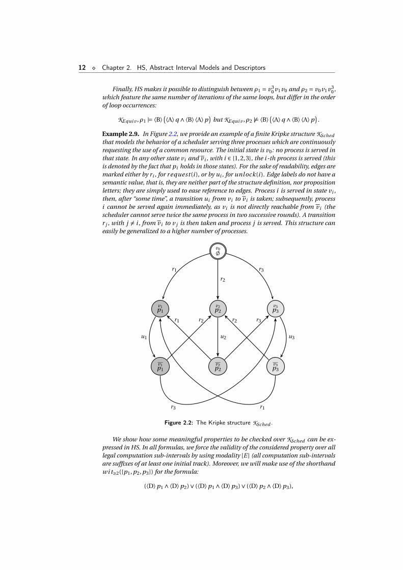
Example 2.9. In Figure 2.2, we provide an example of a finite Kripke structure KSched
that models the behavior of a scheduler serving three processes which are continuouslyrequesting the use of a common resource. The initial state is v0: no process is served inthat state. In any other state vi and v i , with i ∈ 1,2,3, the i -th process is served (thisis denoted by the fact that pi holds in those states). For the sake of readability, edges aremarked either by ri , for r equest (i ), or by ui , for unlock(i ). Edge labels do not have asemantic value, that is, they are neither part of the structure definition, nor propositionletters; they are simply used to ease reference to edges. Process i is served in state vi ,then, after “some time”, a transition ui from vi to v i is taken; subsequently, processi cannot be served again immediately, as vi is not directly reachable from v i (thescheduler cannot serve twice the same process in two successive rounds). A transitionr j , with j 6= i , from v i to v j is then taken and process j is served. This structure caneasily be generalized to a higher number of processes.
v0;
v2p2
v1p1
v3p3
v1p1
v2p2
v3p3
r1
r2
r3
u1 u2 u3
r2
r3
r1 r3
r1
r2
Figure 2.2: The Kripke structure KSched .
We show how some meaningful properties to be checked over KSched can be ex-pressed in HS. In all formulas, we force the validity of the considered property over alllegal computation sub-intervals by using modality [E ] (all computation sub-intervalsare suffixes of at least one initial track). Moreover, we will make use of the shorthandwi t≥2(p1, p2, p3) for the formula:
(⟨D⟩p1 ∧⟨D⟩p2)∨ (⟨D⟩p1 ∧⟨D⟩p3)∨ (⟨D⟩p2 ∧⟨D⟩p3),
2.3. The fundamental notion of BEk -descriptor ¦ 13
which states that there exist at least two sub-intervals such that pi holds over theformer and p j over the latter, with i , j ∈ 1,2,3 and j 6= i (such a formula can be easilygeneralized to an arbitrary set of proposition letters and to any natural number k).The truth of the following statements can be easily checked:
• KSched |= [E ](⟨B⟩5>→ wi t≥2(p1, p2, p3)
);
• KSched 6|= [E ](⟨B⟩10>→⟨D⟩p3
);
• KSched 6|= [E ](⟨B⟩7>→⟨D⟩p1 ∧⟨D⟩p2 ∧⟨D⟩p3
).
The first formula states that in any suffix of an initial track of length greater thanor equal to 7 at least 2 proposition letters are witnessed. KSched satisfies the formulasince a process cannot be executed twice in a row. The second formula states that inany suffix of an initial track of length at least 12 process 3 is executed at least once insome internal states. KSched does not satisfy the formula since the scheduler can avoidexecuting a process ad libitum. The third formula states that in any suffix of an initialtrack of length greater than or equal to 9, p1, p2, p3 are all witnessed. The only wayto satisfy this property is to constrain the scheduler to execute the three processes in astrictly periodic manner, but this is not the case.
2.3 The fundamental notion of BEk-descriptorIn the previous section, we have shown that, for any given finite Kripke structureK , one can find a corresponding induced abstract interval model AK , featuring oneinterval for each track of K . Since K has loops (each state must have at least onesuccessor), the number of its tracks, and thus the number of intervals of AK , is infinite.In this section, we show that, given a finite Kripke structure K and an HS formula ϕ,we can build a finite abstract interval model, which—as we will prove in Chapter 3—isequivalent to AK with respect to the satisfiability ofϕ (in fact, of a class of HS formulasincluding ϕ).
We start with the definition of some basic notions. The first one is the BE-nestingdepth of an HS formula.
Definition 2.10. Let ψ be an HS formula. The BE-nesting depth of ψ, denoted byNestBE(ψ), is defined by induction on the structural complexity of the formula asfollows:
• NestBE(p) = 0, for any proposition letter p ∈ AP ;
• NestBE(¬ψ) = NestBE(ψ);
• NestBE(ψ∧φ) = maxNestBE(ψ),NestBE(φ);
• NestBE(⟨B⟩ψ) = NestBE(⟨E⟩ψ) = 1+NestBE(ψ);
• NestBE(⟨X⟩ψ) = NestBE(ψ), for X ∈ A, A,B ,E .
Making use of the notion of BE-nesting depth of a formula, we can define arelation of k-equivalence over tracks.
Definition 2.11. Let K be a finite Kripke structure and ρ and ρ′ be two tracks in TrkK .We say that ρ and ρ′ are k-equivalent if and only if, for every HS-formula ψ withNestBE(ψ) = k, K ,ρ |=ψ if and only if K ,ρ′ |=ψ.
14 ¦ Chapter 2. HS, Abstract Interval Models and Descriptors
It can be easily proved that k-equivalence propagates downwards.
Proposition 2.12. Let K be a finite Kripke structure and ρ and ρ′ be two tracks inTrkK . If ρ and ρ′ are k-equivalent, then they are h-equivalent, for all 0 ≤ h ≤ k.
Proof. Let us assume that K ,ρ |=ψ, with 0 ≤ NestBE(ψ) ≤ k. Consider the formula⟨B⟩k >, whose BE-nesting depth is equal to k. It trivially holds that either K ,ρ |=⟨B⟩k > or K ,ρ |= ¬⟨B⟩k >. In the first case, we have that K ,ρ |= ⟨B⟩k >∧ψ. SinceNestBE
(⟨B⟩k >∧ψ) = k, from the hypothesis it follows that K ,ρ′ |= ⟨B⟩k >∧ψ, andthus K ,ρ′ |=ψ. The other case can be dealt with in a symmetric way.
We are now ready to introduce the notion of descriptor, which will play a funda-mental role in the definition of finite abstract interval models.
Definition 2.13. A B-descriptor (resp., E-descriptor) is a labeled tree D = (V ,E ,λ),where V is a finite set of vertices, E ⊆V ×V is a set of edges, and λ : V 7→W ×2W ×Wis a node labeling function, that satisfies the following conditions:
1. for all (v, v ′) ∈ E, with λ(v) = (vi n ,S, v f i n) and λ(v ′) = (v ′i n ,S′, v ′
f i n), it holds
that S′ ⊆ S, vi n = v ′i n , and v ′
f i n ∈ S (resp., S′ ⊆ S, v f i n = v ′f i n , and v ′
i n ∈ S);
2. for all pairs of edges (v, v ′), (v, v ′′) ∈ E, if the subtree rooted in v ′ is isomorphic tothe subtree rooted in v ′′, then v ′ = v ′′ (here and in the following, we write subtreefor maximal subtree).
Condition (2) of Definition 2.13 simply states that no two subtrees, whose rootsare siblings, can be isomorphic.
For X ∈ B ,E , the depth of an X -descriptor (V ,E ,λ) is the depth of the tree (V ,E ).We call an X -descriptor of depth k ∈N an Xk -descriptor. An X0-descriptor D consistsof its root only, which is denoted by root(D). A label of a node will be referred toas a descriptor element. Hereafter, two descriptors will be considered equal up toisomorphism. The following lemma holds.
Lemma 2.14. For all k ∈ N, there exists a finite number of possible Bk -descriptors(resp., Ek -descriptors).
Proof. Let us consider the case of Bk -descriptors (the case of Ek -descriptors is anal-ogous). For k = 0, there are at most |W | ·2|W | · |W | pairwise distinct B0-descriptors.As for the inductive step, let us assume h to be the number of pairwise distinct B-descriptors of depth at most k. The number of Bk+1-descriptors is at most |W | ·2|W | ·|W | ·2h (there are at most |W | ·2|W | · |W | possible choices for the root, which can haveany subset of the h B-descriptors of depth at most k as subtrees). Moreover, by theKönig’s lemma, they are all finite, because their depth is k +1 and the root has a finitenumber of children (no two subtrees of the root can be isomorphic).
Lemma 2.14 provides an upper bound to the number of distinct Bk -descriptors(resp., Ek -descr.), and thus to the number of nodes of each Bk+1-descriptor (resp.,Ek+1-descriptors), for k ∈N, which is not elementary with respect to |W | and k, |W |being the exponent and k the height of the exponential tower. As a matter of fact, thisis a very rough upper bound, as some descriptors may not have depth k +1 and someothers might not even fulfil the definition of descriptor.
We show now how B-descriptors and E-descriptors can be exploited to extractrelevant information from the tracks of a finite Kripke structure to be used in model
2.3. The fundamental notion of BEk -descriptor ¦ 15
checking. Let K be a finite Kripke structure and ρ be a track in TrkK . We now describehow to build such descriptors for ρ.
For any k ≥ 0, the label of the root of both the Bk -descriptor and Ek -descriptorfor ρ is the triple (fst(ρ), intstates(ρ), lst(ρ)). The root of the Bk -descriptor has a childfor each prefix ρ′ of ρ, labeled with (fst(ρ′), intstates(ρ′), lst(ρ′)). Such a constructionis then iteratively applied to the children of the root until either depth k is reachedor a track of length 2 is being considered on a node. The Ek -descriptor is built in asimilar way by considering the suffixes of ρ.
In general, B- and E-descriptors do not convey enough information to determinewhich track they were built from (this will be clear shortly). However, they can beexploited to determine which HS formulas are satisfied by the track from which theyhave been built:
• to check satisfiability of proposition letters, they keep information about initial,final, and internal states of the track;
• to deal with ⟨A⟩ψ and ⟨A⟩ψ formulas they store the final and initial states ofthe track;
• to deal with ⟨B⟩ψ formulas, the B-descriptor keeps information about all theprefixes of the track;
• to deal with ⟨E⟩ψ formulas, the E-descriptor keeps information about all thesuffixes of the track;
• no additional information is needed for ⟨B⟩ψ and ⟨E⟩ψ formulas.
Let K be a finite Kripke structure. The Bk -descriptor (resp., Ek -descriptor) for atrack ρ in TrkK is formally defined as follows.
Definition 2.15. Let K be a finite Kripke structure, ρ be a track in TrkK , and k ∈N.The Bk -descriptor (respectively, Ek -descriptor) for ρ is inductively defined as follows:
• for k = 0, the Bk -descriptor (respectively, Ek -descriptor) for ρ is the tree
D = (root(D),;,λ),
whereλ(root(D)) = (fst(ρ), intstates(ρ), lst(ρ));
• for k > 0, the Bk -descriptor (respectively, Ek -descriptor) for ρ is the tree
D = (V ,E ,λ),
whereλ(root(D)) = (fst(ρ), intstates(ρ), lst(ρ)),
which satisfies the following conditions:
1. for each prefix (respectively, suffix) ρ′ of ρ, there exists v ∈ V such that(root(D), v) ∈ E and the subtree rooted in v is the Bk−1-descriptor (respec-tively, Ek−1-descriptor) for ρ′.
2. for each vertex v ∈V such that (root(D), v) ∈ E, there exists a prefix (respec-tively, suffix) ρ′ of ρ such that the subtree rooted in v is the Bk−1-descriptor(respectively, Ek−1-descriptor) for ρ′;
16 ¦ Chapter 2. HS, Abstract Interval Models and Descriptors
3. for all pairs of edges (root(D), v ′), (root(D), v ′′) ∈ E, if the subtree rooted inv ′ is isomorphic to the subtree rooted in v ′′, then v ′ = v ′′.
It can be easily checked that any Bk -descriptor (resp., Ek -descriptor) for sometrack of some finite Kripke structure satisfies the conditions of Definition 2.13 (inparticular, condition (1)), but not vice versa.
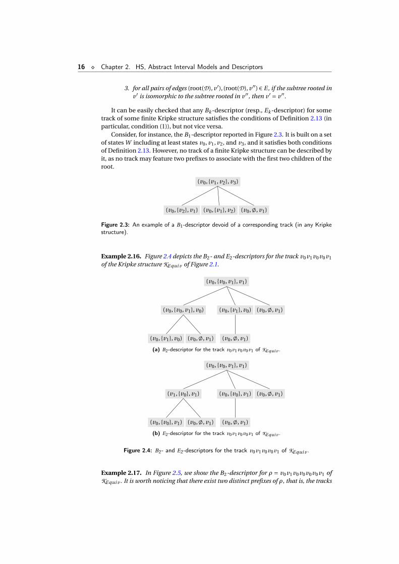
Consider, for instance, the B1-descriptor reported in Figure 2.3. It is built on a setof states W including at least states v0, v1, v2, and v3, and it satisfies both conditionsof Definition 2.13. However, no track of a finite Kripke structure can be described byit, as no track may feature two prefixes to associate with the first two children of theroot.
(v0, v1, v2, v3)
(v0,;, v1)(v0, v1, v2)(v0, v2, v1)
Figure 2.3: An example of a B1-descriptor devoid of a corresponding track (in any Kripkestructure).
Example 2.16. Figure 2.4 depicts the B2- and E2-descriptors for the track v0v1v0v0v1
of the Kripke structure KE qui v of Figure 2.1.
(v0, v0, v1, v1)
(v0,;, v1)(v0, v1, v0)
(v0,;, v1)
(v0, v0, v1, v0)
(v0,;, v1)(v0, v1, v0)
(a) B2-descriptor for the track v0v1v0v0v1 of KE qui v .
(v0, v0, v1, v1)
(v0,;, v1)(v0, v0, v1)
(v0,;, v1)
(v1, v0, v1)
(v0,;, v1)(v0, v0, v1)
(b) E2-descriptor for the track v0v1v0v0v1 of KE qui v .
Figure 2.4: B2- and E2-descriptors for the track v0v1v0v0v1 of KE qui v .
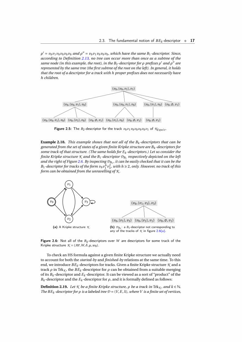
Example 2.17. In Figure 2.5, we show the B2-descriptor for ρ = v0v1v0v0v0v0v1 ofKE qui v . It is worth noticing that there exist two distinct prefixes of ρ, that is, the tracks
2.3. The fundamental notion of BEk -descriptor ¦ 17
ρ′ = v0v1v0v0v0v0 and ρ′′ = v0v1v0v0v0, which have the same B1-descriptor. Since,according to Definition 2.13, no tree can occur more than once as a subtree of thesame node (in this example, the root), in the B2-descriptor for ρ prefixes ρ′ and ρ′′ arerepresented by the same tree (the first subtree of the root on the left). In general, it holdsthat the root of a descriptor for a track with h proper prefixes does not necessarily haveh children.
(v0, v0, v1, v1)
(v0,;, v1)(v0, v1, v0)
(v0,;, v1)
(v0, v0, v1, v0)
(v0,;, v1)(v0, v1, v0)
(v0, v0, v1, v0)
(v0,;, v1)(v0, v1, v0)(v0, v0, v1, v0)
Figure 2.5: The B2-descriptor for the track v0v1v0v0v0v0v1 of KE qui v .
Example 2.18. This example shows that not all of the Bk -descriptors that can begenerated from the set of states of a given finite Kripke structure are Bk -descriptors forsome track of that structure. (The same holds for Ek -descriptors.) Let us consider thefinite Kripke structure K and the B1-descriptor DB1 respectively depicted on the leftand the right of Figure 2.6. By inspecting DB1 , it can be easily checked that it can be theB1-descriptor for tracks of the form v0vh
1 v23 , with h ≥ 2, only. However, no track of this
form can be obtained from the unravelling of K .
v1
v0
v2
v3
(a) A Kripke structure K .
(v0, v1, v3, v3)
(v0,;, v1)(v0, v1, v1)(v0, v1, v3)
(b) DB1 : a B1-descriptor not corresponding toany of the tracks of K in figure 2.6(a).
Figure 2.6: Not all of the Bk -descriptors over W are descriptors for some track of theKripke structure K = (AP ,W,δ,µ, w0).
To check an HS formula against a given finite Kripke structure we actually needto account for both the started-by and finished-by relations at the same time. To thisend, we introduce BEk -descriptors for tracks. Given a finite Kripke structure K and atrack ρ in TrkK , the BEk -descriptor for ρ can be obtained from a suitable mergingof its Bk -descriptor and Ek -descriptor. It can be viewed as a sort of “product” of theBk -descriptor and the Ek -descriptor for ρ, and it is formally defined as follows:
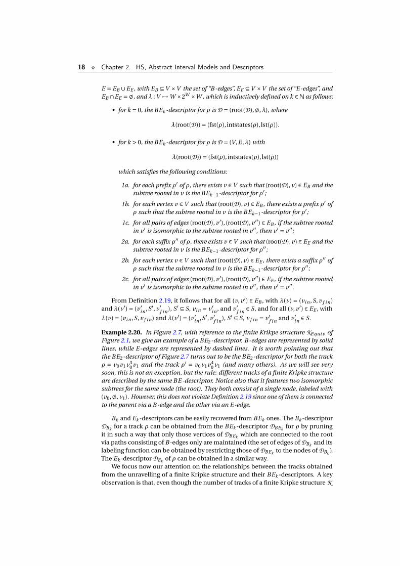
Definition 2.19. Let K be a finite Kripke structure, ρ be a track in TrkK , and k ∈N.The BEk -descriptor for ρ is a labeled tree D = (V ,E ,λ), where V is a finite set of vertices,
18 ¦ Chapter 2. HS, Abstract Interval Models and Descriptors
E = EB ∪EE , with EB ⊆V ×V the set of “B-edges”, EE ⊆V ×V the set of “E-edges”, andEB ∩EE =;, and λ : V 7→W ×2W ×W , which is inductively defined on k ∈N as follows:
• for k = 0, the BEk -descriptor for ρ is D = (root(D),;,λ), where
λ(root(D)) = (fst(ρ), intstates(ρ), lst(ρ)).
• for k > 0, the BEk -descriptor for ρ is D = (V ,E ,λ) with
λ(root(D)) = (fst(ρ), intstates(ρ), lst(ρ))
which satisfies the following conditions:
1a. for each prefix ρ′ of ρ, there exists v ∈V such that (root(D), v) ∈ EB and thesubtree rooted in v is the BEk−1-descriptor for ρ′;
1b. for each vertex v ∈V such that (root(D), v) ∈ EB , there exists a prefix ρ′ ofρ such that the subtree rooted in v is the BEk−1-descriptor for ρ′;
1c. for all pairs of edges (root(D), v ′), (root(D), v ′′) ∈ EB , if the subtree rootedin v ′ is isomorphic to the subtree rooted in v ′′, then v ′ = v ′′;
2a. for each suffix ρ′′ of ρ, there exists v ∈V such that (root(D), v) ∈ EE and thesubtree rooted in v is the BEk−1-descriptor for ρ′′;
2b. for each vertex v ∈V such that (root(D), v) ∈ EE , there exists a suffix ρ′′ ofρ such that the subtree rooted in v is the BEk−1-descriptor for ρ′′;
2c. for all pairs of edges (root(D), v ′), (root(D), v ′′) ∈ EE , if the subtree rootedin v ′ is isomorphic to the subtree rooted in v ′′, then v ′ = v ′′.
From Definition 2.19, it follows that for all (v, v ′) ∈ EB , with λ(v) = (vi n ,S, v f i n)and λ(v ′) = (v ′
i n ,S′, v ′f i n), S′ ⊆ S, vi n = v ′
i n , and v ′f i n ∈ S, and for all (v, v ′) ∈ EE , with
λ(v) = (vi n ,S, v f i n) and λ(v ′) = (v ′i n ,S′, v ′
f i n), S′ ⊆ S, v f i n = v ′f i n and v ′
i n ∈ S.
Example 2.20. In Figure 2.7, with reference to the finite Krikpe structure KE qui v ofFigure 2.1, we give an example of a BE2-descriptor. B-edges are represented by solidlines, while E-edges are represented by dashed lines. It is worth pointing out thatthe BE2-descriptor of Figure 2.7 turns out to be the BE2-descriptor for both the trackρ = v0v1v3
0 v1 and the track ρ′ = v0v1v40 v1 (and many others). As we will see very
soon, this is not an exception, but the rule: different tracks of a finite Kripke structureare described by the same BE-descriptor. Notice also that it features two isomorphicsubtrees for the same node (the root). They both consist of a single node, labeled with(v0,;, v1). However, this does not violate Definition 2.19 since one of them is connectedto the parent via a B-edge and the other via an E-edge.
Bk and Ek -descriptors can be easily recovered from BEk ones. The Bk -descriptorDBk for a track ρ can be obtained from the BEk -descriptor DBEk for ρ by pruningit in such a way that only those vertices of DBEk which are connected to the rootvia paths consisting of B-edges only are maintained (the set of edges of DBk and itslabeling function can be obtained by restricting those of DBEk to the nodes of DBk ).The Ek -descriptor DEk of ρ can be obtained in a similar way.
We focus now our attention on the relationships between the tracks obtainedfrom the unravelling of a finite Kripke structure and their BEk -descriptors. A keyobservation is that, even though the number of tracks of a finite Kripke structure K

2.3. The fundamental notion of BEk -descriptor ¦ 19
(v0
,v 0
,v1
,v 1
)
(v0
,;,v
1)
(v0
,v 0
,v 1
)
(v0
,;,v
1)
(v0
,;,v
0)
(v0
,v 0
,v 1
)
(v0
,;,v
1)
(v0
,v 0
,v 1
)(v
0,;
,v0
)(v
0,
v 0,
v 0)
(v1
,v 0
,v 1
)
(v0
,;,v
1)
(v0
,v 0
,v 1
)(v
1,;
,v0
)(v
1,
v 0,
v 0)
(v0
,;,v
1)
(v0
,v 1
,v 0
)
(v1
,;,v
0)
(v0
,;,v
1)
(v0
,v 0
,v1
,v 0
)
(v0
,;,v
0)
(v1
,v 0
,v 0
)(v
0,;
,v1
)(v
0,
v 1,
v 0)
(v0
,v 0
,v1
,v 0
)
(v0
,;,v
0)
(v0
,v 0
,v 0
)(v
1,
v 0,
v 0)
(v0
,;,v
1)
(v0
,v 1
,v 0
)(v
0,
v 0,v
1,
v 0)
Figu
re2.
7:Anexam
pleof
BE
2-descriptor.
20 ¦ Chapter 2. HS, Abstract Interval Models and Descriptors
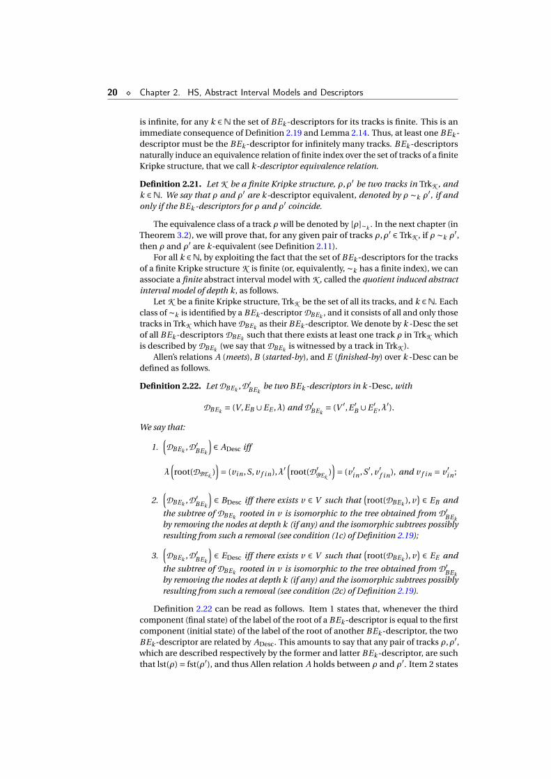
is infinite, for any k ∈N the set of BEk -descriptors for its tracks is finite. This is animmediate consequence of Definition 2.19 and Lemma 2.14. Thus, at least one BEk -descriptor must be the BEk -descriptor for infinitely many tracks. BEk -descriptorsnaturally induce an equivalence relation of finite index over the set of tracks of a finiteKripke structure, that we call k-descriptor equivalence relation.
Definition 2.21. Let K be a finite Kripke structure, ρ,ρ′ be two tracks in TrkK , andk ∈N. We say that ρ and ρ′ are k-descriptor equivalent, denoted by ρ ∼k ρ
′, if andonly if the BEk -descriptors for ρ and ρ′ coincide.
The equivalence class of a track ρ will be denoted by [ρ]∼k . In the next chapter (inTheorem 3.2), we will prove that, for any given pair of tracks ρ,ρ′ ∈ TrkK , if ρ ∼k ρ
′,then ρ and ρ′ are k-equivalent (see Definition 2.11).
For all k ∈N, by exploiting the fact that the set of BEk -descriptors for the tracksof a finite Kripke structure K is finite (or, equivalently, ∼k has a finite index), we canassociate a finite abstract interval model with K , called the quotient induced abstractinterval model of depth k, as follows.
Let K be a finite Kripke structure, TrkK be the set of all its tracks, and k ∈N. Eachclass of ∼k is identified by a BEk -descriptor DBEk , and it consists of all and only thosetracks in TrkK which have DBEk as their BEk -descriptor. We denote by k -Desc the setof all BEk -descriptors DBEk such that there exists at least one track ρ in TrkK whichis described by DBEk (we say that DBEk is witnessed by a track in TrkK ).
Allen’s relations A (meets), B (started-by), and E (finished-by) over k -Desc can bedefined as follows.
Definition 2.22. Let DBEk ,D ′BEk
be two BEk -descriptors in k -Desc, with
DBEk = (V ,EB ∪EE ,λ) and D ′BEk
= (V ′,E ′B ∪E ′
E ,λ′).
We say that:
1.(DBEk ,D ′
BEk
)∈ ADesc iff
λ(root(DBEk )
)= (vi n ,S, v f i n),λ′
(root(D ′
BEk))= (v ′
i n ,S′, v ′f i n), and v f i n = v ′
i n ;
2.(DBEk ,D ′
BEk
)∈ BDesc iff there exists v ∈ V such that
(root(DBEk ), v
) ∈ EB and
the subtree of DBEk rooted in v is isomorphic to the tree obtained from D ′BEk
by removing the nodes at depth k (if any) and the isomorphic subtrees possiblyresulting from such a removal (see condition (1c) of Definition 2.19);
3.(DBEk ,D ′
BEk
)∈ EDesc iff there exists v ∈ V such that
(root(DBEk ), v
) ∈ EE and
the subtree of DBEk rooted in v is isomorphic to the tree obtained from D ′BEk
by removing the nodes at depth k (if any) and the isomorphic subtrees possiblyresulting from such a removal (see condition (2c) of Definition 2.19).
Definition 2.22 can be read as follows. Item 1 states that, whenever the thirdcomponent (final state) of the label of the root of a BEk -descriptor is equal to the firstcomponent (initial state) of the label of the root of another BEk -descriptor, the twoBEk -descriptor are related by ADesc. This amounts to say that any pair of tracks ρ,ρ′,which are described respectively by the former and latter BEk -descriptor, are suchthat lst(ρ) = fst(ρ′), and thus Allen relation A holds between ρ and ρ′. Item 2 states

2.3. The fundamental notion of BEk -descriptor ¦ 21
that, whenever there exists a subtree of DBEk , linked to the root via a B-edge, whichis isomorphic to the tree obtained from D ′
BEkby removing the nodes at depth k (if
any) and the isomorphic subtrees possibly resulting from such a removal (this is thecase, for instance, with subtrees of D ′
BEkthat differ on the labels of nodes at depth k
only), DBEk and D ′BEk
are related by BDesc. As a matter of fact, several tracks may bedescribed by the same BEk -descriptor DBEk . However, whenever a track is describedby (the tree obtained from the pruning of) D ′
BEk, it is a prefix of at least one of the
tracks described by DBEk . Item 3 is analogous to item 2.The generalization of Definition 2.22 to pairs of descriptors belonging to k -Desc
and k ′ -Desc, with k 6= k ′, is straightforward.We are now ready to formally define the notion of quotient induced abstract
interval model of depth k.
Definition 2.23. Let K = (AP ,W,δ,µ, v0) be a finite Kripke structure, ϕ be an HSformula with BE-nesting depth k ∈N, and
Ω= ⋃h≤k
h -Desc.
The quotient induced abstract interval model of depth k is the finite abstract intervalmodel A/∼k = (AP ,Ω, ADesc,BDesc,EDesc,σ), where the valuation functionσ :Ω 7→ 2AP
is such that for all DBE ∈Ω, with λ(root(DBE )) = (vi n ,S, v f i n),
σ(DBE ) =µ(vi n)∩ ⋂v∈S
µ(v)∩µ(v f i n).
This notion is fundamental for the decidability of the model checking problemfor HS, which is proved in the next chapter.


3Decidability of model checking
for HS andEXPSPACE-hardness
Contents3.1 The decidability proof . . . . . . . . . . . . . . . . . . . . . . . . . . 233.2 k-equivalence and corresponding BEk -descriptors . . . . . . . . . 263.3 EXPSPACE-hardness of HS model checking . . . . . . . . . . . . . 31
In this chapter we prove the decidability of the model checking problem for HSover finite Kripke structures (under the homogeneity assumption). The proof makesan essential use of quotient induced abstract interval models. Formally, we show that,for any given finite Kripke structure K , the (finite) quotient induced abstract intervalmodel A/∼k and the (possibly infinite) abstract interval model AK , induced by K ,are equivalent with respect to the satisfiability of HS formulas with nesting depthat most k. In addition, we show that the notions of k-equivalence and k-descriptorequivalence are not equivalent (if two tracks are k-descriptor equivalent, they arealso k-equivalent, but not vice versa), and we show how to weaken the notion ofk-descriptor equivalence to perfectly match k-equivalence.
Finally, we prove that the model checking problem for HS against finite Kripkestructures is EXPSPACE-hard, if a suitable succinct encoding of formulas is exploited,otherwise it is PSPACE-hard.
3.1 The decidability proof
As a preliminary step, we prove a right extension lemma. Let K be a finite Kripkestructure, k ∈N, and ρ and ρ′ be two tracks in TrkK with the same BEk -descriptor(and thus, in particular, lst(ρ) = lst(ρ′)). The lemma states that if we extend ρ and ρ′
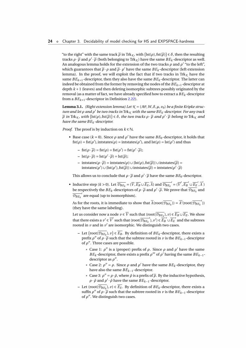
24 ¦ Chapter 3. Decidability of model checking for HS and EXPSPACE-hardness
“to the right” with the same track ρ in TrkK , with(lst(ρ), fst(ρ)
) ∈ δ, then the resultingtracks ρ ·ρ and ρ′ ·ρ (both belonging to TrkK ) have the same BEk -descriptor as well.An analogous lemma holds for the extension of the two tracks ρ and ρ′ “to the left”,which guarantees that ρ ·ρ and ρ ·ρ′ have the same BEk -descriptor (left extensionlemma). In the proof, we will exploit the fact that if two tracks in TrkK have thesame BEk+1-descriptor, then they also have the same BEk -descriptor. The latter canindeed be obtained from the former by removing the nodes of the BEk+1-descriptor atdepth k +1 (leaves) and then deleting isomorphic subtrees possibly originated by theremoval (as a matter of fact, we have already specified how to extract a BEk -descriptorfrom a BEk+1-descriptor in Definition 2.22).
Lemma 3.1. (Right extension lemma) Let K = (AP ,W,δ,µ, v0) be a finite Kripke struc-ture and let ρ and ρ′ be two tracks in TrkK with the same BEk -descriptor. For any trackρ in TrkK , with
(lst(ρ), fst(ρ)
) ∈ δ, the two tracks ρ ·ρ and ρ′ ·ρ belong to TrkK andhave the same BEk -descriptor.
Proof. The proof is by induction on k ∈N.
• Base case (k = 0). Since ρ and ρ′ have the same BE0-descriptor, it holds thatfst(ρ) = fst(ρ′), intstates(ρ) = intstates(ρ′), and lst(ρ) = lst(ρ′) and thus
– fst(ρ ·ρ) = fst(ρ) = fst(ρ′) = fst(ρ′ ·ρ);
– lst(ρ ·ρ) = lst(ρ′ ·ρ) = lst(ρ);
– intstates(ρ ·ρ) = intstates(ρ)∪ lst(ρ), fst(ρ)∪ intstates(ρ) =intstates(ρ′)∪ lst(ρ′), fst(ρ)∪ intstates(ρ) = intstates(ρ′ ·ρ)
This allows us to conclude that ρ ·ρ and ρ′ ·ρ have the same BE0-descriptor.
• Inductive step (k > 0). Let DBEk = (V ,EB ∪EE ,λ) and DBEk
′ = (V′,EB
′∪EE′,λ
′)
be respectively the BEk -descriptors of ρ ·ρ and ρ′ ·ρ. We prove that DBEk and
DBEk
′are equal (up to isomorphism).
As for the roots, it is immediate to show that λ(root(DBEk )) = λ′(root(DBEk
′))
(they have the same labeling).
Let us consider now a node v ∈V such that (root(DBEk ), v) ∈ EB ∪EE . We show
that there exists a v ′ ∈V′
such that (root(DBEk
′), v ′) ∈ EB
′∪EE′
and the subtreesrooted in v and in v ′ are isomorphic. We distinguish two cases.
– Let(root(DBEk ), v
) ∈ EB . By definition of BEk -descriptor, there exists aprefix ρ′′ of ρ ·ρ such that the subtree rooted in v is the BEk−1-descriptorof ρ′′. Three cases are possible.
* Case 1: ρ′′ is a (proper) prefix of ρ. Since ρ and ρ′ have the sameBEk -descriptor, there exists a prefix ρ′′′ of ρ′ having the same BEk−1-descriptor as ρ′′.
* Case 2: ρ′′ = ρ. Since ρ and ρ′ have the same BEk -descriptor, theyhave also the same BEk−1-descriptor.
* Case 3: ρ′′ = ρ ·ρ, where ρ is a prefix of ρ. By the inductive hypothesis,ρ · ρ and ρ′ · ρ have the same BEk−1-descriptor.
– Let (root(DBEk ), v) ∈ EE . By definition of BEk -descriptor, there exists asuffix ρ′′ of ρ ·ρ such that the subtree rooted in v is the BEk−1-descriptorof ρ′′. We distinguish two cases.
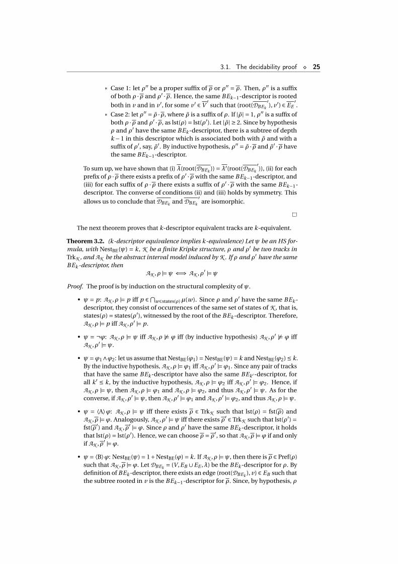
3.1. The decidability proof ¦ 25
* Case 1: let ρ′′ be a proper suffix of ρ or ρ′′ = ρ. Then, ρ′′ is a suffixof both ρ ·ρ and ρ′ ·ρ. Hence, the same BEk−1-descriptor is rooted
both in v and in v ′, for some v ′ ∈V′
such that (root(DBEk
′), v ′) ∈ EE
′.
* Case 2: let ρ′′ = ρ ·ρ, where ρ is a suffix of ρ. If |ρ| = 1, ρ′′ is a suffix ofboth ρ ·ρ and ρ′ ·ρ, as lst(ρ) = lst(ρ′). Let |ρ| ≥ 2. Since by hypothesisρ and ρ′ have the same BEk -descriptor, there is a subtree of depthk −1 in this descriptor which is associated both with ρ and with asuffix of ρ′, say, ρ′. By inductive hypothesis, ρ′′ = ρ ·ρ and ρ′ ·ρ havethe same BEk−1-descriptor.
To sum up, we have shown that (i) λ(root(DBEk )) =λ′(root(DBEk
′)), (ii) for each
prefix of ρ ·ρ there exists a prefix of ρ′ ·ρ with the same BEk−1-descriptor, and(iii) for each suffix of ρ ·ρ there exists a suffix of ρ′ ·ρ with the same BEk−1-descriptor. The converse of conditions (ii) and (iii) holds by symmetry. This
allows us to conclude that DBEk and DBEk
′are isomorphic.
The next theorem proves that k-descriptor equivalent tracks are k-equivalent.
Theorem 3.2. (k-descriptor equivalence implies k-equivalence) Let ψ be an HS for-mula, with NestBE(ψ) = k, K be a finite Kripke structure, ρ and ρ′ be two tracks inTrkK , and AK be the abstract interval model induced by K . If ρ and ρ′ have the sameBEk -descriptor, then
AK ,ρ |=ψ ⇐⇒ AK ,ρ′ |=ψProof. The proof is by induction on the structural complexity of ψ.
• ψ = p: AK ,ρ |= p iff p ∈ ⋂w∈states(ρ)µ(w). Since ρ and ρ′ have the same BEk -
descriptor, they consist of occurrences of the same set of states of K , that is,states(ρ) = states(ρ′), witnessed by the root of the BEk -descriptor. Therefore,AK ,ρ |= p iff AK ,ρ′ |= p.
• ψ = ¬ϕ: AK ,ρ |= ψ iff AK ,ρ 6|= ϕ iff (by inductive hypothesis) AK ,ρ′ 6|= ϕ iffAK ,ρ′ |=ψ.
• ψ=ϕ1∧ϕ2: let us assume that NestBE(ϕ1) = NestBE(ψ) = k and NestBE(ϕ2) ≤ k.By the inductive hypothesis, AK ,ρ |=ϕ1 iff AK ,ρ′ |=ϕ1. Since any pair of tracksthat have the same BEk -descriptor have also the same BEk ′-descriptor, forall k ′ ≤ k, by the inductive hypothesis, AK ,ρ |= ϕ2 iff AK ,ρ′ |= ϕ2. Hence, ifAK ,ρ |= ψ, then AK ,ρ |= ϕ1 and AK ,ρ |= ϕ2, and thus AK ,ρ′ |= ψ. As for theconverse, if AK ,ρ′ |=ψ, then AK ,ρ′ |=ϕ1 and AK ,ρ′ |=ϕ2, and thus AK ,ρ |=ψ.
• ψ = ⟨A⟩ϕ: AK ,ρ |= ψ iff there exists ρ ∈ TrkK such that lst(ρ) = fst(ρ) andAK ,ρ |=ϕ. Analogously, AK ,ρ′ |=ψ iff there exists ρ′ ∈ TrkK such that lst(ρ′) =fst(ρ′) and AK ,ρ′ |=ϕ. Since ρ and ρ′ have the same BEk -descriptor, it holdsthat lst(ρ) = lst(ρ′). Hence, we can choose ρ = ρ′, so that AK ,ρ |=ϕ if and onlyif AK ,ρ′ |=ϕ.
• ψ= ⟨B⟩ϕ: NestBE(ψ) = 1+NestBE(ϕ) = k. If AK ,ρ |=ψ, then there is ρ ∈ Pref(ρ)such that AK ,ρ |=ϕ. Let DBEk = (V ,EB ∪EE ,λ) be the BEk -descriptor for ρ. Bydefinition of BEk -descriptor, there exists an edge (root(DBEk ), v) ∈ EB such thatthe subtree rooted in v is the BEk−1-descriptor for ρ. Since, by hypothesis, ρ
26 ¦ Chapter 3. Decidability of model checking for HS and EXPSPACE-hardness
and ρ′ have the same BEk -descriptor, there exists a prefix ρ′ of ρ′ such thatthe subtree rooted in v is the BEk−1-descriptor for ρ′. Now, by the inductivehypothesis, AK ,ρ′ |=ϕ, and thus AK ,ρ′ |=ψ. Exactly the same argument allowsus to conclude that if AK ,ρ′ |=ψ, then AK ,ρ |=ψ.
• ψ = ⟨B⟩ϕ: if AK ,ρ |=ψ, then there exists ρ in TrkK such that ρ ∈ Pref(ρ) andAK ,ρ |=ϕ. We can express ρ as ρ ·ρ for some ρ in TrkK such that (lst(ρ), fst(ρ)) ∈δ. Now, since ρ and ρ′ have the same BEk -descriptor, it holds that lst(ρ) =lst(ρ′). By Lemma 3.1, ρ = ρ · ρ and ρ′ · ρ have the same BEk -descriptor. Bythe inductive hypothesis, AK ,ρ′ · ρ |=ϕ, and thus AK ,ρ′ |=ψ. Exactly the sameargument allows us to conclude that if AK ,ρ′ |=ψ, then AK ,ρ |=ψ.
The remaining cases can be proven by symmetry.
Since k-descriptor equivalence preserves satisfiability of HS formulas, testingwhether K ,ρ |=ψ can be reduced to checking whether A/∼k , [ρ]∼k |=ψ.
Corollary 3.3. Let ψ be an HS formula, with NestBE(ψ) ≤ k, K be a finite Kripkestructure, and ρ be a track in TrkK . It holds that
K ,ρ |=ψ ⇐⇒ A/∼k , [ρ]∼k |=ψ.
Proof. By Definition 2.6, K ,ρ |=ψ if and only if AK ,ρ |=ψ. The proof of the left-to-right implication (if AK ,ρ |=ψ, then A/∼k , [ρ]∼k |=ψ) is by induction on the structuralcomplexity of ψ, and it basically makes use of Definition 2.22 and Definition 2.23.The proof of the opposite implication is straightforward.
By exploiting Corollary 3.3, we can reduce the model checking problem for HSagainst finite Kripke structures to the model checking problem for multi-modal, finiteKripke structures, whose nodes are all possible (witnessed) descriptors, with depthup to k, and there is a distinct accessibility relation for each one of the HS modalitiesA, B , E , A, B , and E . Since the model checking problem for multi-modal, finiteKripke structures and formulas is decidable (in [Gab87, Lan06], it has been shownthat the model checking problem for multi-modal Kripke structures and formulasis decidable in polynomial time with respect to both the size of the Kripke structureand the length of the formula), decidability of the model checking problem for HSagainst finite Kripke structures immediately follows.
Theorem 3.4. The model checking problem for HS against finite Kripke structures isdecidable (with a non-elementary algorithm).
Proof. Lemma 2.14 provides a non-elementary upper bound to the number of BEh-descriptors, with 0 ≤ h ≤ k, as well as to the size of BEk+1-descriptors, with respectto the size of the Kripke structure and the nesting depth k of the input HS formula.Hence, the derived model checking problem for multi-modal, finite Kripke structureshas to be solved over a model whose size has a non-elementary upper bound.
3.2 The relation between k-equivalence and cor-responding BEk-descriptors
In the previous section (in Theorem 3.2), we prove that k-descriptor equivalenceis a sufficient condition for k-equivalence, that is, if two tracks are k-descriptor
3.2. k-equivalence and corresponding BEk -descriptors ¦ 27
equivalent, then they are k-equivalent. However, it is not a necessary one. To showthat the converse does not hold, consider once more the finite Kripke structureKE qui v in Figure 2.1. The tracks v5
0 and v60 of KE qui v have the same BE2-descriptor,
but not the same BE3-descriptor, yet there exists no formula ψ, with NestBE(ψ) ≤ 3,such that K , v6
0 |=ψ and K , v50 6|=ψ. Intuitively, since these two tracks are made of
a different number of occurrences of the same state, the only way to distinguishthem is by means of the formula ⟨B⟩4>, or similar ones, for which K , v6
0 |= ⟨B⟩4> andK , v5
0 6|= ⟨B⟩4>, but these formulas have a BE-nesting depth greater than 3.In the following, we introduce the notion of corresponding BEk -descriptors, and
we prove that it provides a necessary and sufficient condition for k-equivalence.Such a notion allows us to rephrase equivalence between tracks in terms of moreabstract characteristics of their descriptors, in a stronger way than Theorem 3.2. Asan example, by exploiting the correspondence among descriptors it defines and thestatement of Theorem 3.11 below, it will be possible to prove that v5
0 and v60 are
actually 3-equivalent.
Definition 3.5. Let K = (AP ,W,δ,µ, w0) be a finite Kripke structure, let DBEk andD ′
BEkbe two BEk -descriptors associated with some of its tracks, and let (vi n ,S, v f i n)
and (v ′i n ,S′, v ′
f i n) be the labels of the root of DBEk and D ′BEk
, respectively. We say that
DBEk and D ′BEk
are corresponding BEk -descriptors if and only if:
• the two roots are labelled by the same set of propositions, that is,⋂w∈vi n ∪S∪v f i n
µ(w) = ⋂w ′∈v ′
i n ∪S′∪v ′f i n
µ(w ′);
• for any track ρ ∈ TrkK , with fst(ρ) = v f i n , there is a track ρ′ ∈ TrkK with fst(ρ′) =v ′
f i n , such that ρ and ρ′ are associated with corresponding BEk -descriptors, and
vice versa (we say that the BEk -descriptors for ρ and ρ′ are A-successors of DBEk
and D ′BEk
, respectively);
• for any track ρ ∈ TrkK , with lst(ρ) = vi n , there is a track ρ′ ∈ TrkK , with lst(ρ′) =v ′
i n , such that ρ and ρ′ are associated with corresponding BEk -descriptors, and
vice versa (we say that the BEk -descriptors for ρ and ρ′ are A-successors of DBEk
and D ′BEk
, respectively);
• given a track ρ associated with DBEk and a track ρ′ associated with D ′BEk
, for
any track ρ, with (v f i n , fst(ρ)) ∈ δ, there is a track ρ′, with (v ′f i n , fst(ρ′)) ∈ δ,
such that both ρ ·ρ and ρ′ ·ρ′ belong to TrkK , and they are associated withcorresponding BEk -descriptors, and vice versa (we say that the BEk -descriptorsfor ρ ·ρ and ρ′ ·ρ′ are B-successors of DBEk and D ′
BEk, respectively)1;
• given a track ρ associated with DBEk and a track ρ′ associated with D ′BEk
, for any
track ρ, with (lst(ρ), vi n) ∈ δ, there is a track ρ′, with (lst(ρ′), v ′i n) ∈ δ, such that
both ρ · ρ and ρ′ · ρ′ belong to TrkK , and they are associated with correspondingBEk -descriptors, and vice versa (we say that the BEk -descriptors for ρ · ρ andρ′ · ρ′ are E-successors of DBEk and D ′
BEk, respectively);
1If a track ρ was considered in place of ρ and they are both associated with DBEk, by the right extension
lemma ρ ·ρ ∈ TrkK and ρ ·ρ ∈ TrkK are associated with the same descriptor as well.
28 ¦ Chapter 3. Decidability of model checking for HS and EXPSPACE-hardness
• whenever k > 0, for any subtree of depth k −1 in DBEk , whose root is linked tothe root of DBEk via a B-edge, there is a corresponding subtree of depth k −1 inD ′
BEk, whose root is linked to the root of D ′
BEkvia a B-edge, and vice versa;
• whenever k > 0, for any subtree of depth k−1 in DBEk , whose root is linked to theroot of DBEk via an E-edge, there exists a corresponding subtree of depth k −1 inD ′
BEk, whose root is linked to the root of D ′
BEkvia an E-edge, and vice versa.
It can easily be checked that the correspondence between descriptors of Defi-nition 3.5 is an equivalence relation. Definition 3.5 expresses a form of bisimula-tion among BEk -descriptors with respect to the defined relations of A-successor,A-successor, B-successor, B-successor, E-successor, and E-successor. Since, in afinite Kripke structure, every state has (at least) a successor with respect to δ, BEk -descriptors always have both A-successors and B-successors. On the contrary, BEk -descriptors may have no A-successors or E-successors, because a state does notnecessarily have a predecessor with respect to δ, Finally, a BEk -descriptor has B- andE-successors if and only if k ≥ 1 and the represented tracks are long enough. Thenumber of proper prefixes (resp., suffixes) of short tracks can indeed be less than k.In such a case, the actual height of BEk -descriptors is less than the nominal heightk, and thus it may happen that the BEi -descriptor and BE j -descriptor, with i 6= j ,for a track are isomorphic. When collecting all the BEi -descriptor, for 0 ≤ i ≤ k (forinstance, in Definition 3.6 below), isomorphic descriptors of different depths will beconsidered as distinct elements.
The set of descriptors and their successor relations, corresponding to the variousHS modalities, allow us to define a graph structure.
Definition 3.6. Let K = (AP ,W,δ,µ, w0) be a finite Kripke structure. The graph G ofthe BE-descriptors of depth at most k, with k ≥ 0, witnessed by some tracks of K , is apair (VG ,EG ), where EG ⊆VG ×VG is a set of labeled edges, such that:
• VG contains a node for each BEt -descriptor, with 0 ≤ t ≤ k, witnessed by sometrack of K ;
• edges in EG are labeled with X ∈ A,B ,E , A,B ,E according to the followingcriteria:
– (v, v ′) ∈ EG is an X -edge, with X ∈ A, A,B ,E , whenever the descriptor ofv ′ is an X -successor of the descriptor of v;
– (v, v ′) ∈ EG is a B-edge whenever the descriptors associated with v and v ′are DBEt and D ′
BEt−1, respectively (for some t ≥ 1), and D ′
BEt−1is isomorphic
to a subtree of DBEt connected to the root of DBEt via a B-edge;
– (v, v ′) ∈ EG is an E-edge whenever the descriptors associated with v and v ′are DBEt and D ′
BEt−1, respectively (for some t ≥ 1), and D ′
BEt−1is isomorphic
to a subtree of DBEt connected to the root of DBEt via an E-edge.
The set of nodes VG is finite and the out-degree of every node is finite as well.Moreover, VG can be partitioned into k sets, according to the depth of the descriptorsassociated with its nodes. A node associated with a descriptor of depth t can beconnected to a node associated with a descriptor of depth t −1, with 0 < t ≤ k, onlyby B- or E-edges. It is possible to show that two descriptors are corresponding ifand only if the associated nodes in the graph are bisimilar. Thus, the definition of
3.2. k-equivalence and corresponding BEk -descriptors ¦ 29
correspondence between descriptors could be equivalently expressed in terms of astandard notion of bisimilarity among nodes of G .
For technical reasons, we need to introduce a variant of two of the previously-defined concepts: the nesting depth of formulas, to take into consideration thenesting of all HS modalities (not only B and E as in Definition 2.10), and descriptorcorrespondence up to a bounded number of “steps”.
Definition 3.7. The nesting depth of an HS formula ψ, denoted by Nest(ψ), is induc-tively defined on the structure of ψ as follows:
• Nest(p) = 0, for any proposition letter p ∈ AP ;
• Nest(¬ψ) = Nest(ψ);
• Nest(ψ∧φ) = maxNest(ψ),Nest(φ);
• Nest(⟨X⟩ψ) = 1+Nest(ψ), with X ∈ A,B ,E , A,B ,E .
It trivially holds that NestBE(ψ) ≤ Nest(ψ) for all formulas ψ.The next definition differs from Definition 3.5 in the limitation to a bounded
number of coinductive steps that it introduces in the descriptor correspondence.
Definition 3.8. Let K = (AP ,W,δ,µ, w0) be a finite Kripke structure, let DBEk andD ′
BEkbe two BEk -descriptors associated with some of its tracks, and let (vi n ,S, v f i n)
and (v ′i n ,S′, v ′
f i n) be the labels of the root of DBEk and D ′BEk
, respectively. We say that
DBEk and D ′BEk
are corresponding BEk -descriptors up to depth n if and only if:
• the two roots are labeled by the same set of propositions, that is,⋂w∈vi n ∪S∪v f i n
µ(w) = ⋂w ′∈v ′
i n ∪S′∪v ′f i n
µ(w ′);
• if n > 0:
– for any track ρ ∈ TrkK , with fst(ρ) = v f i n , there is a track ρ′ ∈ TrkK , withfst(ρ′) = v ′
f i n , such that ρ and ρ′ are associated with corresponding BEk -
descriptors up to depth n −1, and vice versa;
– for any track ρ ∈ TrkK , with lst(ρ) = vi n , there is a track ρ′ ∈ TrkK , withlst(ρ′) = v ′
i n , such that ρ and ρ′ are associated with corresponding BEk -descriptors up to depth n −1, and vice versa;
– given two tracks ρ and ρ′ associated with DBEk and D ′BEk
, respectively, for
any track ρ, with (v f i n , fst(ρ)) ∈ δ, there is a track ρ′, with (v ′f i n , fst(ρ′)) ∈ δ,
such that both ρ ·ρ and ρ′ ·ρ′ belong to TrkK , and they are associated withcorresponding BEk -descriptors up to depth n −1, and vice versa;
– given two tracks ρ and ρ′ associated with DBEk and D ′BEk
, respectively, for
any track ρ, with (lst(ρ), vi n) ∈ δ, there is a track ρ′, with (lst(ρ′), v ′i n) ∈ δ,
such that both ρ · ρ and ρ′ · ρ′ belong to TrkK , and they are associated withcorresponding BEk -descriptors up to depth n −1, and vice versa;
– whenever k > 0, for any subtree of depth k −1 in DBEk , whose root is linkedto the root of DBEk via a B-edge (resp. E-edge), there is a subtree of depthk −1 in D ′
BEk, whose root is linked to the root of D ′
BEkvia a B-edge (resp.,
E-edge), corresponding up to depth n −1, and vice versa.
30 ¦ Chapter 3. Decidability of model checking for HS and EXPSPACE-hardness
In order to prove that corresponding descriptors actually capture the notion of k-equivalence (Theorem 3.11 below), we need a couple of preparatory lemmas, whoseproofs are given in the appendix (Section A.1).
Lemma 3.9. Let K = (AP ,W,δ,µ, w0) be a finite Kripke structure and ρ,ρ′ be twotracks in TrkK . For all n,k ∈N, with k ≤ n, if ρ and ρ′ are k-equivalent with respectto all HS formulas ψ, with Nest(ψ) ≤ n, then the BEk -descriptors of ρ and ρ′ arecorresponding up to depth n.
Lemma 3.10. Let K = (AP ,W,δ,µ, w0) be a finite Kripke structure. For all n,k ∈ N,with k ≥ 1, if two descriptors DBEk and D ′
BEkare corresponding up to depth n, then
DBEk |k−1 and D ′BEk
|k−1 are corresponding up to depth n, where DBEk |k−1 denotes thedescriptor obtained from DBEk by deleting its nodes at depth k (and removing possibleisomorphic subtrees).
The following theorem formally states the relationship between correspondingdescriptors and track equivalence.
Theorem 3.11. Let K be a finite Kripke structure, k ∈N, and ρ,ρ′ ∈ TrkK . The tracksρ and ρ′ are k-equivalent if and only if ρ and ρ′ are associated with correspondingBEk -descriptors.
Proof. (⇒) Let us first show that if ρ and ρ′ are k-equivalent, then they are associatedwith corresponding BEk -descriptors. The proof directly follows from Lemma 3.9.Since ρ and ρ′ are k-equivalent, with no bound on the nesting depth of formulas,then their BEk -descriptors are corresponding, with no bound on the depth.
(⇐) We now prove that, for any HS formula ψ, with NestBE(ψ) = k, if ρ and ρ′ areassociated with corresponding BEk -descriptors, then K ,ρ |=ψ ⇐⇒ K ,ρ′ |=ψ. Theproof is by induction on the structure of the formula.
• Let K ,ρ |= p, for some p ∈ AP . Since the roots for the BE-descriptors of ρ andρ′ are labeled with the same set of proposition letters, it immediately followsthat K ,ρ′ |= p.
• Let K ,ρ |=ψ1 ∧ψ2. Then, K ,ρ |=ψ1 and K ,ρ |=ψ2. Let NestBE(ψ1) = k andassume w.l.o.g. that NestBE(ψ2) = t ≤ k. By Definition 3.8 and Lemma 3.10,it immediately follows that if ρ and ρ′ have corresponding BEk -descriptors,then they also have corresponding BEt -descriptors, with t ≤ k. Hence, bythe inductive hypothesis, K ,ρ′ |=ψ1 and K ,ρ′ |=ψ2, and, as a consequence,K ,ρ′ |=ψ1 ∧ψ2.
• Let K ,ρ |= ¬ψ. Then, K ,ρ 6|=ψ. By the inductive hypothesis, K ,ρ′ 6|=ψ, andthus K ,ρ′ |= ¬ψ.
• Let K ,ρ |= ⟨A⟩ψ. Then, there exists a track ρ ∈ TrkK , with fst(ρ) = lst(ρ), suchthat K ,ρ |= ψ. Since the BEk -descriptors for ρ and ρ′ are corresponding,there exists, in particular, a track ρ′ ∈ TrkK , with fst(ρ′) = lst(ρ′), such thatthe BEk -descriptors for ρ and ρ′ are corresponding. By the inductive hypothe-sis, K ,ρ′ |=ψ, so K ,ρ′ |= ⟨A⟩ψ. The ⟨A⟩ case is symmetric (notice that, due tothe correspondence of the BEk -descriptors for ρ and ρ′, there exists ρ ∈ TrkK ,with lst(ρ) = fst(ρ), if and only if there exists ρ′ ∈ TrkK , with lst(ρ′) = fst(ρ′)).
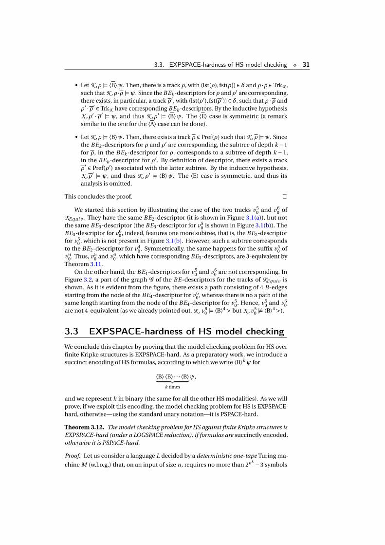
3.3. EXPSPACE-hardness of HS model checking ¦ 31
• Let K ,ρ |= ⟨B⟩ψ. Then, there is a track ρ, with (lst(ρ), fst(ρ)) ∈ δ and ρ ·ρ ∈ TrkK ,such that K ,ρ·ρ |=ψ. Since the BEk -descriptors for ρ and ρ′ are corresponding,there exists, in particular, a track ρ′, with (lst(ρ′), fst(ρ′)) ∈ δ, such that ρ ·ρ andρ′ ·ρ′ ∈ TrkK have corresponding BEk -descriptors. By the inductive hypothesisK ,ρ′ ·ρ′ |= ψ, and thus K ,ρ′ |= ⟨B⟩ψ. The ⟨E⟩ case is symmetric (a remarksimilar to the one for the ⟨A⟩ case can be done).
• Let K ,ρ |= ⟨B⟩ψ. Then, there exists a track ρ ∈ Pref(ρ) such that K ,ρ |=ψ. Sincethe BEk -descriptors for ρ and ρ′ are corresponding, the subtree of depth k −1for ρ, in the BEk -descriptor for ρ, corresponds to a subtree of depth k − 1,in the BEk -descriptor for ρ′. By definition of descriptor, there exists a trackρ′ ∈ Pref(ρ′) associated with the latter subtree. By the inductive hypothesis,K ,ρ′ |= ψ, and thus K ,ρ′ |= ⟨B⟩ψ. The ⟨E⟩ case is symmetric, and thus itsanalysis is omitted.
This concludes the proof.
We started this section by illustrating the case of the two tracks v50 and v6
0 ofKE qui v . They have the same BE2-descriptor (it is shown in Figure 3.1(a)), but notthe same BE3-descriptor (the BE3-descriptor for v5
0 is shown in Figure 3.1(b)). TheBE3-descriptor for v6
0 , indeed, features one more subtree, that is, the BE2-descriptorfor v5
0 , which is not present in Figure 3.1(b). However, such a subtree correspondsto the BE2-descriptor for v4
0 . Symmetrically, the same happens for the suffix v50 of
v60 . Thus, v5
0 and v60 , which have corresponding BE3-descriptors, are 3-equivalent by
Theorem 3.11.On the other hand, the BE4-descriptors for v5
0 and v60 are not corresponding. In
Figure 3.2, a part of the graph G of the BE-descriptors for the tracks of KE qui v isshown. As it is evident from the figure, there exists a path consisting of 4 B-edgesstarting from the node of the BE4-descriptor for v6
0 , whereas there is no a path of thesame length starting from the node of the BE4-descriptor for v5
0 . Hence, v50 and v6
0are not 4-equivalent (as we already pointed out, K , v6
0 |= ⟨B⟩4> but K , v50 6|= ⟨B⟩4>).
3.3 EXPSPACE-hardness of HS model checking
We conclude this chapter by proving that the model checking problem for HS overfinite Kripke structures is EXPSPACE-hard. As a preparatory work, we introduce asuccinct encoding of HS formulas, according to which we write ⟨B⟩k ψ for
⟨B⟩⟨B⟩ · · · ⟨B⟩︸ ︷︷ ︸k times
ψ,
and we represent k in binary (the same for all the other HS modalities). As we willprove, if we exploit this encoding, the model checking problem for HS is EXPSPACE-hard, otherwise—using the standard unary notation—it is PSPACE-hard.
Theorem 3.12. The model checking problem for HS against finite Kripke structures isEXPSPACE-hard (under a LOGSPACE reduction), if formulas are succinctly encoded,otherwise it is PSPACE-hard.
Proof. Let us consider a language L decided by a deterministic one-tape Turing ma-
chine M (w.l.o.g.) that, on an input of size n, requires no more than 2nk −3 symbols
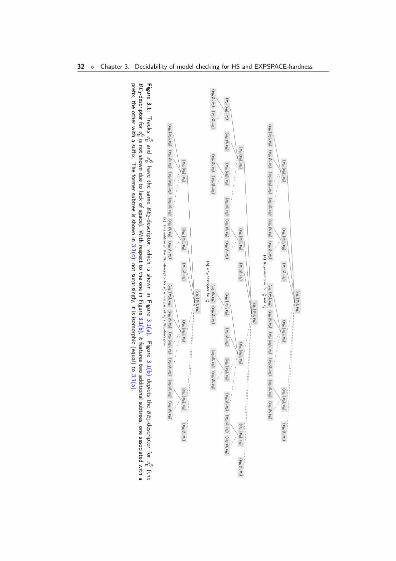
32 ¦ Chapter 3. Decidability of model checking for HS and EXPSPACE-hardness
(v0 ,v
0 ,v0 )
(v0 ,;
,v0 )
(v0 ,v
0 ,v0 )
(v0 ,;
,v0 )
(v0 ,;
,v0 )
(v0 ,v
0 ,v0 )
(v0 ,;
,v0 )
(v0 ,v
0 ,v0 )
(v0 ,;
,v0 )
(v0 ,v
0 ,v0 )
(v0 ,;
,v0 )
(v0 ,v
0 ,v0 )
(v0 ,;
,v0 )
(v0 ,;
,v0 )
(v0 ,v
0 ,v0 )
(v0 ,;
,v0 )
(v0 ,v
0 ,v0 )
(v0 ,;
,v0 )
(v0 ,v
0 ,v0 )
(a)B
E2 -descriptor
forv
50and
v60 .
(v0 ,v
0 ,v0 )
(v0 ,;
,v0 )
(v0 ,v
0 ,v0 )
(v0 ,;
,v0 )
(v0 ,;
,v0 )
(v0 ,v
0 ,v0 )
(v0 ,;
,v0 )
(v0 ,v
0 ,v0 )
(v0 ,;
,v0 )
(v0 ,;
,v0 )
(v0 ,;
,v0 )
(v0 ,v
0 ,v0 )
(v0 ,;
,v0 )
(v0 ,;
,v0 )
(v0 ,;
,v0 )
(v0 ,v
0 ,v0 )
(v0 ,;
,v0 )
(v0 ,;
,v0 )
(v0 ,v
0 ,v0 )
(v0 ,;
,v0 )
(v0 ,v
0 ,v0 )
(v0 ,;
,v0 )
(v0 ,;
,v0 )
(v0 ,;
,v0 )
(v0 ,v
0 ,v0 )
(v0 ,;
,v0 )
(v0 ,;
,v0 )
(b)B
E3 -descriptor
forv
50 .
(v0 ,v
0 ,v0 )
(v0 ,;
,v0 )
(v0 ,v
0 ,v0 )
(v0 ,;
,v0 )
(v0 ,;
,v0 )
(v0 ,v
0 ,v0 )
(v0 ,;
,v0 )
(v0 ,v
0 ,v0 )
(v0 ,;
,v0 )
(v0 ,v
0 ,v0 )
(v0 ,;
,v0 )
(v0 ,v
0 ,v0 )
(v0 ,;
,v0 )
(v0 ,;
,v0 )
(v0 ,v
0 ,v0 )
(v0 ,;
,v0 )
(v0 ,v
0 ,v0 )
(v0 ,;
,v0 )
(v0 ,v
0 ,v0 )
(c)This
subtreeof
theB
E3 -descriptor
forv
60isnot
partof
v50 ’s
BE
3 -descriptor.
Figure3.1:
Tracks
v50and
v60have
thesam
eB
E2 -descriptor,
which
isshow
nin
Figure3.1(a).
Figure3.1(b)
depictsthe
BE
3 -descriptorfor
v50(the
BE
3 -descriptorfor
v60isnot
showndue
tolack
ofspace).
With
respectto
theone
inFigure
3.1(b),itfeatures
twoadditionalsubtrees,
oneassociated
with
aprefix,
theother
with
asuffi
x.The
former
subtreeisshow
nin
3.1(c);not
surprisingly,itisisom
orphic(equal)
to3.1(a).
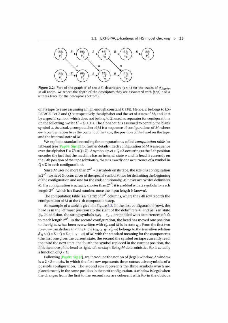
3.3. EXPSPACE-hardness of HS model checking ¦ 33
BE4
v60
BE3
v50
BE2
v40
BE1
v30
BE0
v20
BE4
v50
BE3
v40
BE2
v30
BE1
v20
B B B B
B B B
B B B
Figure 3.2: Part of the graph G of the BEt -descriptors (t ≤ 4) for the tracks of KE qui v .In all nodes, we report the depth of the descriptors they are associated with (top) and awitness track for the descriptor (bottom).
on its tape (we are assuming a high enough constant k ∈N). Hence, L belongs to EX-PSPACE. Let Σ and Q be respectively the alphabet and the set of states of M , and let #be a special symbol, which does not belong to Σ, used as separator for configurations(in the following, we let Σ′ =Σ∪ #). The alphabet Σ is assumed to contain the blanksymbol t. As usual, a computation of M is a sequence of configurations of M , whereeach configuration fixes the content of the tape, the position of the head on the tape,and the internal state of M .
We exploit a standard encoding for computations, called computation table (ortableau) (see [Pap94, Sip12] for further details). Each configuration of M is a sequenceover the alphabet Γ=Σ′∪(Q×Σ). A symbol (q,c) ∈Q×Σ occurring at the i -th positionencodes the fact that the machine has an internal state q and its head is currently onthe i -th position of the tape (obviously, there is exactly one occurrence of a symbol inQ ×Σ in each configuration).
Since M uses no more than 2nk −3 symbols on its tape, the size of a configuration
is 2nk(we need 3 occurrences of the special symbol #, two for delimiting the beginning
of the configuration and one for the end; additionally, M never overwrites delimiters
#). If a configuration is actually shorter than 2nk, it is padded with t symbols to reach
length 2nk(which is a fixed number, once the input length is known).
The computation table is a matrix of 2nkcolumns, where the i -th row records the
configuration of M at the i -th computation step.An example of a table is given in Figure 3.3. In the first configuration (row), the
head is in the leftmost position (to the right of the delimiters #) and M is in stateq0. In addition, the string symbols c0c1 · · ·cn−1 are padded with occurrences of t’s
to reach length 2nk. In the second configuration, the head has moved one position
to the right, c0 has been overwritten with c ′0, and M is in state q1. From the first tworows, we can deduce that the tuple (q0,c0, q1,c ′0,→) belongs to the transition relationδM ⊆Q ×Σ×Q ×Σ× →,←,• of M , with the standard meaning for the components(the first one gives the current state, the second the symbol on tape currently read,the third the next state, the fourth the symbol replaced in the current position, thefifth the move of the head to right, left, or stay). Being M deterministic , δM is actuallya function of Q ×Σ.
Following [Pap94, Sip12], we introduce the notion of (legal) window. A windowis a 2×3 matrix, in which the first row represents three consecutive symbols of apossible configuration. The second row represents the three symbols which areplaced exactly in the same position in the next configuration. A window is legal whenthe changes from the first to the second row are coherent with δM in the obvious
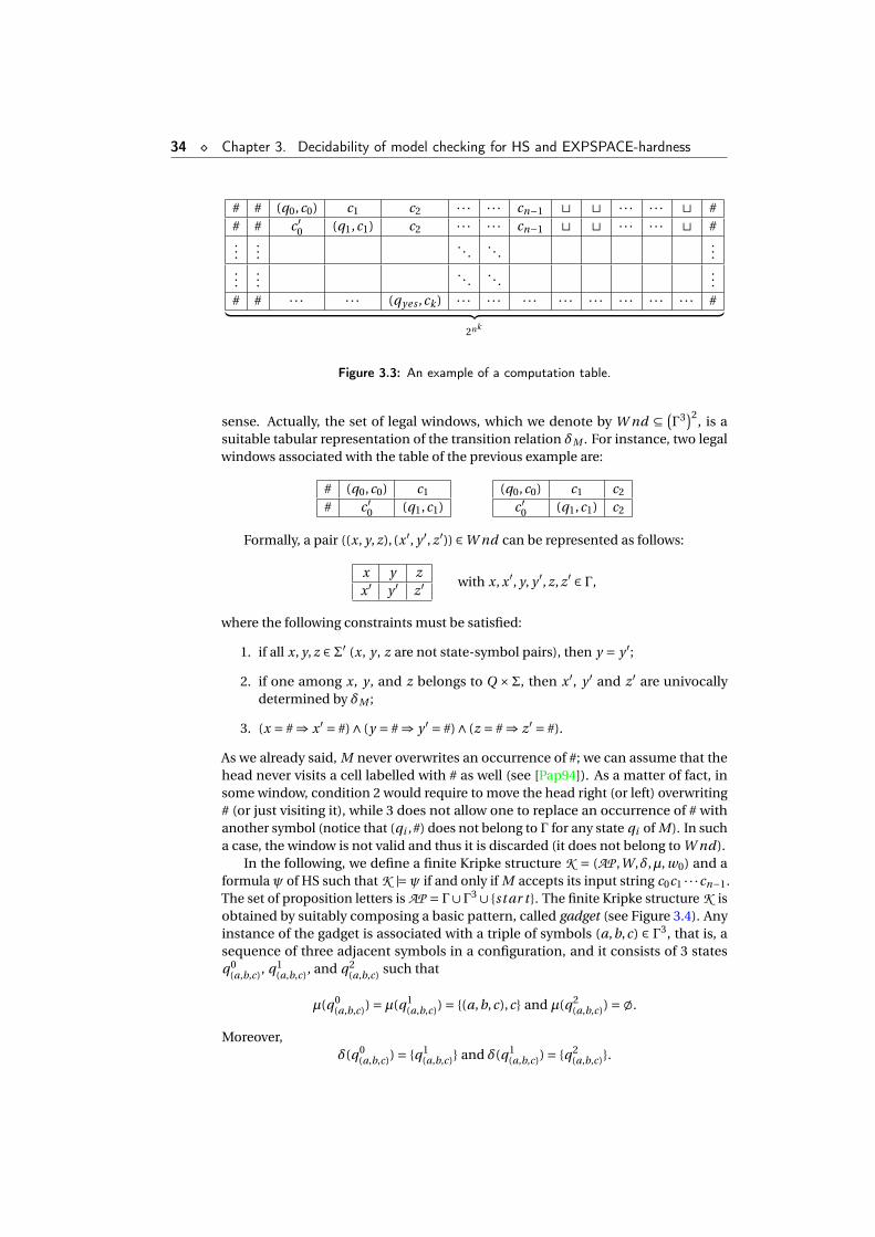
34 ¦ Chapter 3. Decidability of model checking for HS and EXPSPACE-hardness
# # (q0,c0) c1 c2 · · · · · · cn−1 t t ·· · · · · t ## # c ′0 (q1,c1) c2 · · · · · · cn−1 t t ·· · · · · t #...
.... . .
. . ....
......
. . .. . .
...# # · · · · · · (qyes ,ck ) · · · · · · · · · · · · · · · · · · · · · · · · #︸ ︷︷ ︸
2nk
Figure 3.3: An example of a computation table.
sense. Actually, the set of legal windows, which we denote by W nd ⊆ (Γ3
)2, is a
suitable tabular representation of the transition relation δM . For instance, two legalwindows associated with the table of the previous example are:
# (q0,c0) c1
# c ′0 (q1,c1)(q0,c0) c1 c2
c ′0 (q1,c1) c2
Formally, a pair ((x, y, z), (x ′, y ′, z ′)) ∈W nd can be represented as follows:
x y zx ′ y ′ z ′ with x, x ′, y, y ′, z, z ′ ∈ Γ,
where the following constraints must be satisfied:
1. if all x, y, z ∈Σ′ (x, y , z are not state-symbol pairs), then y = y ′;
2. if one among x, y , and z belongs to Q ×Σ, then x ′, y ′ and z ′ are univocallydetermined by δM ;
3. (x = # ⇒ x ′ = #)∧ (y = # ⇒ y ′ = #)∧ (z = # ⇒ z ′ = #).
As we already said, M never overwrites an occurrence of #; we can assume that thehead never visits a cell labelled with # as well (see [Pap94]). As a matter of fact, insome window, condition 2 would require to move the head right (or left) overwriting# (or just visiting it), while 3 does not allow one to replace an occurrence of # withanother symbol (notice that (qi ,#) does not belong to Γ for any state qi of M). In sucha case, the window is not valid and thus it is discarded (it does not belong to W nd).
In the following, we define a finite Kripke structure K = (AP ,W,δ,µ, w0) and aformula ψ of HS such that K |=ψ if and only if M accepts its input string c0c1 · · ·cn−1.The set of proposition letters is AP = Γ∪Γ3 ∪ st ar t . The finite Kripke structure K isobtained by suitably composing a basic pattern, called gadget (see Figure 3.4). Anyinstance of the gadget is associated with a triple of symbols (a,b,c) ∈ Γ3, that is, asequence of three adjacent symbols in a configuration, and it consists of 3 statesq0
(a,b,c), q1(a,b,c), and q2
(a,b,c) such that
µ(q0(a,b,c)) =µ(q1
(a,b,c)) = (a,b,c),c and µ(q2(a,b,c)) =;.
Moreover,δ(q0
(a,b,c)) = q1(a,b,c) and δ(q1
(a,b,c)) = q2(a,b,c).
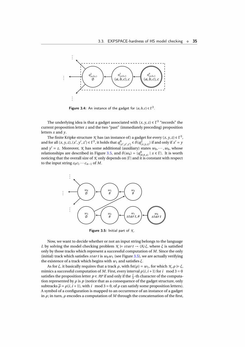
3.3. EXPSPACE-hardness of HS model checking ¦ 35
q0(a,b,c)
(a,b,c),cq1
(a,b,c)
(a,b,c),cq2
(a,b,c);...
...
...
Figure 3.4: An instance of the gadget for (a,b,c) ∈ Γ3.
The underlying idea is that a gadget associated with (x, y, z) ∈ Γ3 “records” thecurrent proposition letter z and the two “past” (immediately preceding) propositionletters x and y .
The finite Kripke structure K has (an instance of) a gadget for every (x, y, z) ∈ Γ3,and for all (x, y, z), (x ′, y ′, z ′) ∈ Γ3, it holds that q0
(x′,y ′,z ′) ∈ δ(q2(x,y,z)) if and only if x ′ = y
and y ′ = z. Moreover, K has some additional (auxiliary) states w0, · · · , w6, whoserelationships are described in Figure 3.5, and δ(w6) = q0
(#,#,x) | x ∈ Γ. It is worthnoticing that the overall size of K only depends on |Γ| and it is constant with respectto the input string c0c1 · · ·cn−1 of M .
w0st ar t
w1st ar t ,#
w2#
w3;
w4#
w5#
w6;...
...
...
Figure 3.5: Initial part of K .
Now, we want to decide whether or not an input string belongs to the languageL by solving the model checking problem K |= st ar t → ⟨A⟩ξ, where ξ is satisfiedonly by those tracks which represent a successful computation of M . Since the only(initial) track which satisfies st ar t is w0w1 (see Figure 3.5), we are actually verifyingthe existence of a track which begins with w1 and satisfies ξ.
As for ξ, it basically requires that a track ρ, with fst(ρ) = w1, for which K ,ρ |= ξ,mimics a successful computation of M . First, every interval ρ(i , i +1) for i mod 3 = 0satisfies the proposition letter p ∈ AP if and only if the i
3 -th character of the computa-tion represented by ρ is p (notice that as a consequence of the gadget structure, onlysubtracks ρ = ρ(i , i +1), with i mod 3 = 0, of ρ can satisfy some proposition letters).A symbol of a configuration is mapped to an occurrence of an instance of a gadgetin ρ; in turn, ρ encodes a computation of M through the concatenation of the first,
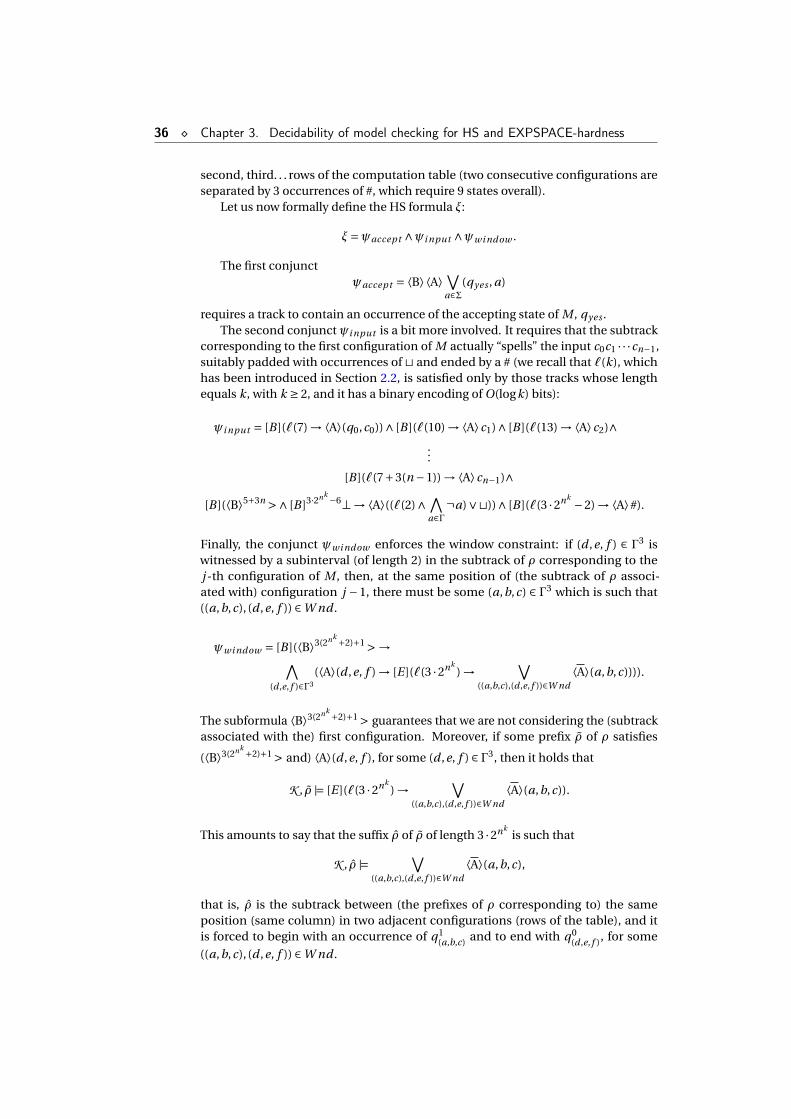
36 ¦ Chapter 3. Decidability of model checking for HS and EXPSPACE-hardness
second, third. . . rows of the computation table (two consecutive configurations areseparated by 3 occurrences of #, which require 9 states overall).
Let us now formally define the HS formula ξ:
ξ=ψaccept ∧ψi nput ∧ψwi ndow .
The first conjunctψaccept = ⟨B⟩⟨A⟩ ∨
a∈Σ(qyes , a)
requires a track to contain an occurrence of the accepting state of M , qyes .The second conjunct ψi nput is a bit more involved. It requires that the subtrack
corresponding to the first configuration of M actually “spells” the input c0c1 · · ·cn−1,suitably padded with occurrences of t and ended by a # (we recall that `(k), whichhas been introduced in Section 2.2, is satisfied only by those tracks whose lengthequals k, with k ≥ 2, and it has a binary encoding of O(logk) bits):
ψi nput = [B ](`(7) →⟨A⟩(q0,c0))∧ [B ](`(10) →⟨A⟩c1)∧ [B ](`(13) →⟨A⟩c2)∧...
[B ](`(7+3(n −1)) →⟨A⟩cn−1)∧
[B ](⟨B⟩5+3n >∧ [B ]3·2nk −6⊥→⟨A⟩((`(2)∧ ∧a∈Γ
¬a)∨t))∧ [B ](`(3 ·2nk −2) →⟨A⟩#).
Finally, the conjunct ψwi ndow enforces the window constraint: if (d ,e, f ) ∈ Γ3 iswitnessed by a subinterval (of length 2) in the subtrack of ρ corresponding to thej -th configuration of M , then, at the same position of (the subtrack of ρ associ-ated with) configuration j −1, there must be some (a,b,c) ∈ Γ3 which is such that((a,b,c), (d ,e, f )) ∈W nd .
ψwi ndow = [B ](⟨B⟩3(2nk +2)+1>→∧(d ,e, f )∈Γ3
(⟨A⟩(d ,e, f ) → [E ](`(3 ·2nk) → ∨
((a,b,c),(d ,e, f ))∈W nd⟨A⟩(a,b,c)))).
The subformula ⟨B⟩3(2nk +2)+1> guarantees that we are not considering the (subtrackassociated with the) first configuration. Moreover, if some prefix ρ of ρ satisfies
(⟨B⟩3(2nk +2)+1> and) ⟨A⟩(d ,e, f ), for some (d ,e, f ) ∈ Γ3, then it holds that
K , ρ |= [E ](`(3 ·2nk) → ∨
((a,b,c),(d ,e, f ))∈W nd⟨A⟩(a,b,c)).
This amounts to say that the suffix ρ of ρ of length 3 ·2nkis such that
K , ρ |= ∨((a,b,c),(d ,e, f ))∈W nd
⟨A⟩(a,b,c),
that is, ρ is the subtrack between (the prefixes of ρ corresponding to) the sameposition (same column) in two adjacent configurations (rows of the table), and itis forced to begin with an occurrence of q1
(a,b,c) and to end with q0(d ,e, f ), for some
((a,b,c), (d ,e, f )) ∈W nd .
3.3. EXPSPACE-hardness of HS model checking ¦ 37
It is immediate to check that all the integers which need to be stored in the
formula are less than or equal to 3 ·2nk +7, and thus O(nk ) bits suffice. This allows usto conclude that the formula can be generated in polynomial time (and logarithmicworking space).
If we do not allow the binary encoding of the exponents, the model checkingproblem for HS formulas is PSPACE-hard (under a LOGSPACE reduction): the proofis the same as before, but in order for the formula ξ to be generated in polynomialtime, we must restrict ourselves to computations of Turing machines using at mostpolynomial space.
In conclusion, in this chapter we have proved that the model checking problemfor HS is decidable, and it is EXPSPACE-hard if a proper succinct encoding of for-mulas is exploited, otherwise it is PSPACE-hard. Actually, we have also proved thatthe fragment HS[A, A,B ,E ] is, again, EXPSPACE-hard if the succinct encoding offormulas is allowed, and PSPACE-hard otherwise, because the formula ξ of the aboveproof does not contain occurrences of B and E modalities.
In the next chapter we shall analyze a pair of fragments whose model checking isfeatured by a lower complexity if compared to that of (full) HS, namely HS[A, A,B ,B ,E ]and HS[A, A,E ,B ,E ].

4A model checking algorithm
based on track representatives
Contents4.1 Descriptor element indistinguishability . . . . . . . . . . . . . . . 404.2 Track representatives . . . . . . . . . . . . . . . . . . . . . . . . . . . 464.3 The model checking algorithm . . . . . . . . . . . . . . . . . . . . . 534.4 NEXP-hardness of model checking for HS[A, A,B ,B ,E ] . . . . . . . 55
In this chapter, we restrict our attention to the fragment HS[A, A,B ,B ,E ] andwe show that the model checking problem for it has a lower complexity (comparedto that of full HS). By symmetry, all the results presented in the next sections areapplicable to HS[A, A,E ,B ,E ], as well.
Since E modality does not occur in formulas of HS[A, A,B ,B ,E ], we shall exploitBk -descriptors instead of BEk -descriptors in the following algorithms; moreoverwe preliminary have to “adapt” some of the notions we have already defined in theprevious chapter to such a fragment:
• the B-nesting depth of an HS[A, A,B ,B ,E ] formula ψ, NestB(ψ), is defined likeNestBE, but it does not account for the E modality.
• Two tracks ρ,ρ′ ∈ TrkK are said k-equivalent if and only if, for every formula ψof HS[A, A,B ,B ,E ] with NestB(ψ) = k, it holds that K ,ρ |=ψ iff K ,ρ′ |=ψ.
• Two tracks ρ,ρ′ ∈ TrkK are k-descriptor equivalent, denoted by ρ ∼k ρ′, if and
only if the Bk -descriptors for ρ and ρ′ coincide.
Next we state a lemma and two propositions, which are preparatory to Theo-rem 4.4.
40 ¦ Chapter 4. A model checking algorithm based on track representatives
Lemma 4.1. Let k ∈N, K = (AP ,W,δ,µ, v0) be a finite Kripke structure and ρ1, ρ′1, ρ2,
ρ′2 be tracks in TrkK such that:
(lst(ρ1), fst(ρ′
1)) ∈ δ,
(lst(ρ2), fst(ρ′
2)) ∈ δ, ρ1 ∼k ρ2 and
ρ′1 ∼k ρ
′2. Then ρ1 ·ρ′
1 ∼k ρ2 ·ρ′2.
The proof can be found in A.2.1. The next propositions immediately follow:
Proposition 4.2. (Right extension) Let K = (AP ,W,δ,µ, v0) be a finite Kripke struc-ture, ρ and ρ′ be two tracks in TrkK such that ρ ∼k ρ
′. For any ρ ∈ TrkK such that(lst(ρ), fst(ρ)
) ∈ δ, it holds that ρ ·ρ ∼k ρ′ ·ρ.
Proposition 4.3. (Left extension) Let K = (AP ,W,δ,µ, v0) be a finite Kripke struc-ture, ρ and ρ′ be two tracks in TrkK such that ρ ∼k ρ
′. For any ρ ∈ TrkK such that(lst(ρ), fst(ρ)
) ∈ δ, it holds that ρ ·ρ ∼k ρ ·ρ′.
The former proposition states that if we extend the two tracks ρ and ρ′ having thesame Bk -descriptor “to the right” with the same track ρ ∈ TrkK , with
(lst(ρ), fst(ρ)
) ∈ δ,then the resulting tracks ρ ·ρ and ρ′ ·ρ (both belonging to TrkK ) have the same Bk -descriptor as well. The latter proposition symmetrically deals with the extension ofthe two tracks ρ and ρ′ “to the left”. In these Propositions 4.2 and 4.3, |ρ| ≥ 2; howeverboth continue to hold if |ρ| = 1.
The following theorem is the analogous to Theorem 3.2 for Bk -descriptors; itsproof is omitted, as it is basically a simplification of that of Theorem 3.2.
Theorem 4.4. Let K be a finite Kripke structure, ρ and ρ′ two tracks in TrkK , AKthe abstract interval model induced by K and ψ a formula of HS[A, A,B ,B ,E ] withNestB(ψ) = k. If ρ ∼k ρ
′, then AK ,ρ |=ψ ⇐⇒ AK ,ρ′ |=ψ.
Thanks to this theorem and to the notions of descriptor element indistinguisha-bility and track representatives presented in the next sections, we will provide anEXPSPACE model checking algorithm for HS[A, A,B ,B ,E ]. Finally, we will provethat the model checking problem for the fragment HS[A, A,B ,B ,E ] is NEXP-hard if asuitable succinct encoding of formulas is exploited.
4.1 Descriptor element indistinguishabilityA Bk -descriptor provides a finite encoding for a possibly infinite set of tracks (thetracks associated with that descriptor). Unfortunately, the representation of Bk -descriptors as trees labelled over descriptor elements is highly redundant. As anexample, given any pair of subtrees rooted in some children of the root of a descriptor,it is always the case that one of them is a subtree of the other. This property immedi-ately follows from the fact that the two subtrees are associated with two (different)prefixes of a track and one of them is necessarily a prefix of the other. In practice, thesize of the tree representation of Bk -descriptors prevents their direct use in modelchecking algorithms, and makes it difficult to determine the intrinsic complexity ofBk -descriptors.
In this section, we devise a more compact representation of Bk -descriptors. Eachclass of the k-descriptor equivalence relation is a set of k-equivalent tracks. For everysuch class, we select a representative track whose length is (exponentially) boundedin both the cardinality of W (the set of states of the Kripke structure) and k.
In order to fix such a bound on the length of track representatives, we considersuitable ordered sequences (possibly with repetitions) of descriptor elements of a Bk -descriptor. Let us define the descriptor sequence for a track as the ordered sequence
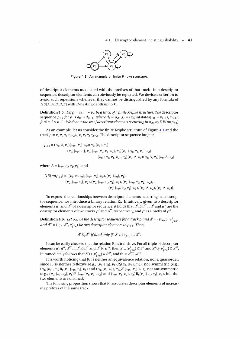
4.1. Descriptor element indistinguishability ¦ 41
v0
v1
v2
v3
Figure 4.1: An example of finite Kripke structure.
of descriptor elements associated with the prefixes of that track. In a descriptorsequence, descriptor elements can obviously be repeated. We devise a criterion toavoid such repetitions whenever they cannot be distinguished by any formula ofHS[A, A,B ,B ,E ] with B-nesting depth up to k.
Definition 4.5. Let ρ = v0v1 · · ·vn be a track of a finite Kripke structure. The descriptorsequence ρd s for ρ is d0 · · ·dn−1, where di = ρd s (i ) = (v0, intstates(v0 · · ·vi+1), vi+1),for 0 ≤ i ≤ n−1. We denote the set of descriptor elements occurring inρd s by DElm(ρd s ).
As an example, let us consider the finite Kripke structure of Figure 4.1 and thetrack ρ = v0v0v0v1v2v1v2v3v3v2v2. The descriptor sequence for ρ is:
ρd s = (v0,;, v0)(v0, v0, v0)(v0, v0, v1)
(v0, v0, v1, v2)(v0, v0, v1, v2, v1)(v0, v0, v1, v2, v2)
(v0, v0, v1, v2, v3)(v0,∆, v3)(v0,∆, v2)(v0,∆, v2)
where ∆= v0, v1, v2, v3, and
DElm(ρd s ) = (v0,;, v0), (v0, v0, v0), (v0, v0, v1),
(v0, v0, v1, v2), (v0, v0, v1, v2, v1), (v0, v0, v1, v2, v2),
(v0, v0, v1, v2, v3), (v0,∆, v2), (v0,∆, v3).
To express the relationships between descriptor elements occurring in a descrip-tor sequence, we introduce a binary relation Rt. Intuitively, given two descriptorelements d ′ and d ′′ of a descriptor sequence, it holds that d ′ Rt d ′′ if d ′ and d ′′ are thedescriptor elements of two tracks ρ′ and ρ′′, respectively, and ρ′ is a prefix of ρ′′.
Definition 4.6. Let ρd s be the descriptor sequence for a track ρ and d ′ = (vi n ,S′, v ′f i n)
and d ′′ = (vi n ,S′′, v ′′f i n) be two descriptor elements in ρd s . Then,
d ′ Rt d ′′ if (and only if) S′∪ v ′f i n ⊆ S′′.
It can be easily checked that the relation Rt is transitive. For all triple of descriptorelements d ′,d ′′,d ′′′, if d ′ Rt d ′′ and d ′′ Rt d ′′′, then S′∪v ′
f i n ⊆ S′′ and S′′∪v ′′f i n ⊆ S′′′.
It immediately follows that S′∪ v ′f i n ⊆ S′′′, and thus d ′ Rt d ′′′.
It is worth noticing that Rt is neither an equivalence relation, nor a quasiorder,since Rt is neither reflexive (e.g., (v0, v0, v1)R t(v0, v0, v1)), nor symmetric (e.g.,(v0, v0, v1)Rt(v0, v0, v1, v1) and (v0, v0, v1, v1)R t(v0, v0, v1)), nor antisymmetric(e.g., (v0, v1, v2, v1)Rt(v0, v1, v2, v2) and (v0, v1, v2, v2)Rt(v0, v1, v2, v1), but thetwo elements are distinct).
The following proposition shows that Rt associates descriptor elements of increas-ing prefixes of the same track.
42 ¦ Chapter 4. A model checking algorithm based on track representatives
Proposition 4.7. Let ρd s be the descriptor sequence for the track ρ = v0v1 · · ·vn . Then,ρd s (i )Rtρd s ( j ) for all 0 ≤ i < j < n.
Proof. ρd s (i ) and ρd s ( j ) are associated with the tracks ρ1 = v0 · · ·vi+1 and ρ2 =v0 · · ·vi+1 · · ·v j+1, respectively, and thus intstates(ρ1)∪ vi+1 ⊆ intstates(ρ2).
We now introduce a distinction between two types of descriptor element.
Definition 4.8. A descriptor element (vi n ,S, v f i n) is a Type-1 descriptor element ifv f i n ∉ S, while it is a Type-2 descriptor element if v f i n ∈ S.
It can easily be checked that a descriptor element d = (vi n ,S, v f i n) is of Type-1 ifand only if Rt is not reflexive in d : (i) if dR t d , then S ∪ v f i n 6⊆ S, and thus v f i n ∉ S,and (ii) if v f i n ∉ S, then dR t d . It follows that a Type-1 descriptor element cannotoccur more than once in a descriptor sequence. On the contrary, Type-2 descriptorelements may occur multiple times in a descriptor sequence, and if a descriptorelement occurs more than once, then it is necessarily of Type-2.
Proposition 4.9. If it holds that both d ′ Rt d ′′ and d ′′ Rt d ′, where d ′ = (vi n ,S′, v ′f i n)
and d ′′ = (vi n ,S′′, v ′′f i n), then v ′
f i n ∈ S′, v ′′f i n ∈ S′′, and S′ = S′′, and thus both d ′ and
d ′′ are Type-2 descriptor elements.
Proof. S′∪ v ′f i n ⊆ S′′ ⊆ S′′∪ v ′′
f i n ⊆ S′ and S′′∪ v ′′f i n ⊆ S′ ⊆ S′∪ v ′
f i n ⊆ S′′.
We are now ready to provide a general characterization of the descriptor sequenceρd s for a track ρ: ρd s is composed of some (maximal) subsequences, consisting ofoccurrences of Type-2 descriptor elements on which Rt is symmetric, separated byoccurrences of Type-1 descriptor elements. Such a characterization can be formalizedby means of the notion of cluster.
Definition 4.10. A cluster C of (Type-2) descriptor elements is a maximal set ofdescriptor elements d1, · · · ,ds ⊆ DElm(ρd s ) such that di Rt d j and d j Rt di for alli , j ∈ 1, · · · , s.
Thanks to maximality, clusters are pairwise disjoint: if C and C ′ are distinctclusters, d ∈ C and d ′ ∈ C ′, either d Rt d ′ and d ′
R t d , or d ′ Rt d and dR t d ′.
Definition 4.11. Let ρd s be a descriptor sequence and C be one of its clusters. Thesubsequence of ρd s associated with C is a subsequence ρd s (i , j ) such that ρd s (i ′) ∈ Cif and only if i ≤ i ′ ≤ j < |ρd s |.
For example, the descriptor sequence ρd s for ρ = v0v0v0v1v2v1v2v3v3v2v2, atrack of the finite Kripke structure in Figure 4.1, is shown again here; subsequencesassociated with clusters are surrounded by boxes (∆= v0, v1, v2, v3):
ρd s = (v0,;, v0) (v0, v0, v0) (v0, v0, v1)
(v0, v0, v1, v2) (v0, v0, v1, v2, v1)(v0, v0, v1, v2, v2)
(v0, v0, v1, v2, v3) (v0,∆, v3)(v0,∆, v2)(v0,∆, v2) .
It is worth observing that:
• the descriptor elements of a cluster C are contiguous (in other words, they forma subsequence), i.e., occurrences of descriptor elements in C are never shuffledwith occurrences of descriptor elements not belonging to C ;
4.1. Descriptor element indistinguishability ¦ 43
• two subsequences associated with two distinct clusters C and C ′ in a descriptorsequence must be separated by at least one occurrence of a Type-1 descriptorelement (intuitively, in order to “leave” a cluster and to enter another one, anew state—not belonging to the set of already met states—must occur in thetrack). Type-1 descriptor elements thus act as “separators”.
While Rt allows us to order any pair of Type-1 descriptor elements, as well as anyType-1 descriptor element with respect to a Type-2 descriptor element, it does not giveany means to order Type-2 descriptor elements belonging to the same cluster. This,together with the fact that Type-2 descriptor elements may have multiple occurrencesin a descriptor sequence, implies that we need to somehow limit the number ofoccurrences of Type-2 descriptor elements in order to give a bound on the length oftrack representatives of Bk -descriptors.
To this end, we introduce an equivalence relation that allows us to put together in-distinguishable occurrences of the same descriptor element in a descriptor sequence,that is, to detect those occurrences which are associated with prefixes of the track withthe same Bk -descriptor. The idea is that a track representative for a Bk -descriptorshould not include indistinguishable occurrences of the same descriptor element.
Definition 4.12. Let ρd s be a descriptor sequence and k ≥ 1. We say that two occur-rences ρd s (i ) and ρd s ( j ), with 0 ≤ i < j < |ρd s |, of the same descriptor element d arek-indistinguishable if (and only if):
• (for k = 1) DElm(ρd s (0, i −1)) = DElm(ρd s (0, j −1));
• (for k ≥ 2) for all i ≤ ` ≤ j −1, there exists 0 ≤ `′ ≤ i −1 such that ρd s (`) andρd s (`′) are (k −1)-indistinguishable.
From Definition 4.12, it immediately follows that two indistinguishable occur-rences ρd s (i ) and ρd s ( j ) of the same descriptor element necessarily belong to thesame subsequence of ρd s .
In general, it is always the case that DElm(ρd s (0, i −1)) ⊆ DEl m(ρd s (0, j −1)),for i < j . Moreover, 1-indistinguishability guarantees that DEl m(ρd s (0, i − 1)) =DElm(ρd s (0, j −1)). From this, it easily follows that the two first occurrences of adescriptor element are not 1-indistinguishable.
Propositions 4.13, 4.14 state some basic properties of the k-indistinguishabilityrelation.
Proposition 4.13. Let k ≥ 2 and ρd s (i ) and ρd s ( j ), with 0 ≤ i < j < |ρd s |, be two k-indistinguishable occurrences of the same descriptor element in a descriptor sequenceρd s . Then, ρd s (i ) and ρd s ( j ) are (k −1)-indistinguishable.
Proof. The proof is by induction on k ≥ 2.Base case (k = 2). Let ρd s (i ) and ρd s ( j ) be two 2-indistinguishable occurrences of
a descriptor element d . By definition, for any ρd s (i ′), with i ≤ i ′ < j , an occurrence ofthe descriptor element d ′ = ρd s (i ′) must occur before position i , and thus
DElm(ρd s (0, i −1)) = DEl m(ρd s (0, j −1)).
It immediately follows that ρd s (i ) and ρd s ( j ) are 1-indistinguishable.Inductive step (k ≥ 3). By definition, for all i ≤ `≤ j −1, there exists 0 ≤ `′ ≤ i −1
such that ρd s (`) and ρd s (`′) are (k−1)-indistinguishable. By the inductive hypothesis,ρd s (`) and ρd s (`′) are (k −2)-indistinguishable, which implies that ρd s (i ) and ρd s ( j )are (k −1)-indistinguishable.
44 ¦ Chapter 4. A model checking algorithm based on track representatives
Proposition 4.14. Let k ≥ 1 and ρd s (i ) and ρd s (m), with 0 ≤ i < m < |ρd s |, be twok-indistinguishable occurrences of the same descriptor element in a descriptor se-quence ρd s . If ρd s ( j ) = ρd s (m), for some i < j < m, then ρd s ( j ) and ρd s (m) arek-indistinguishable.
Proof. The proof is by induction on k ≥ 1.Base case (k = 1). Since DElm(ρd s (0, i −1)) = DElm(ρd s (0,m −1)) and
DElm(ρd s (0, i −1)) ⊆ DElm(ρd s (0, j −1)) ⊆ DElm(ρd s (0,m −1)),
thenDElm(ρd s (0, i −1)) = DElm(ρd s (0,m −1)) = DEl m(ρd s (0, j −1)),
proving the property.Inductive step (k ≥ 2). By hypothesis, all occurrences ρd s (i ′), with i ≤ i ′ < m,
are (k −1)-indistinguishable from some occurrence of the same descriptor elementbefore i . In particular, this is true for all occurrences ρd s ( j ′), with j ≤ j ′ < m. Thethesis trivially follows.
In Figure 4.2, we provide some examples of k-indistinguishability relations, fork ∈ 1,2,3, for a track of the finite Kripke structure depicted in Figure 4.1.
The next theorem establishes a fundamental connection between the notions ofk-indistinguishability of descriptor elements and k-descriptor equivalence of tracks.
Theorem 4.15. Let ρd s be the descriptor sequence for a track ρ. Two occurrences ρd s (i )and ρd s ( j ), 0 ≤ i < j < |ρd s |, of the same descriptor element are k-indistinguishable ifand only if ρ(0, i +1) ∼k ρ(0, j +1).
Proof. Let us assume that ρd s (i ) and ρd s ( j ), with i < j , are k-indistinguishable. Weprove by induction on k ≥ 1 that ρ(0, i +1) and ρ(0, j +1) have the same Bk -descriptor.
Base case (k = 1). Since ρd s (i ) and ρd s ( j ) are occurrences of the same descriptorelement, the B1-descriptors for ρ(0, i +1) and ρ(0, j +1) have roots labeled by thesame descriptor element. Moreover, the children of these B1-descriptors are inone-to-one correspondence since, by 1-indistinguishability, DEl m(ρd s (0, i −1)) =DElm(ρd s (0, j −1)).
Inductive step (k ≥ 2). Since all the prefixes of ρ(0, i + 1) are also prefixes ofρ(0, j +1), we just need to consider the prefixes ρ(0, t ) with i +1 ≤ t ≤ j . By definition,any occurrence ρd s (i ′) with i ≤ i ′ < j , is (k − 1)-indistinguishable from anotheroccurrence ρd s (i ′′), with i ′′ < i , of the same descriptor element. By the inductivehypothesis, ρ(0, i ′+1) and ρ(0, i ′′+1) have the same Bk−1-descriptor. It follows thatfor any proper prefix of ρ(0, j +1) (of length at least 2), there exists a proper prefix ofρ(0, i +1) with the same Bk−1-descriptor, which implies that the tracks ρ(0, i +1) andρ(0, j +1) have the same Bk -descriptor.
Conversely, we prove, by induction on k > 1, that if ρd s (i ) and ρd s ( j ), with i < j ,are not k-indistinguishable, then the Bk -descriptors of ρ(0, i +1) and ρ(0, j +1) aredifferent. We assume ρd s (i ) and ρd s ( j ) to be occurrences of the same descriptorelement (if this was not the case, the thesis would trivially follow, since the roots ofthe Bk -descriptors for ρ(0, i+1) and ρ(0, j+1) would be labeled by different descriptorelements).
Base case (k = 1). If ρd s (i ) and ρd s ( j ), with i < j , are not 1-indistinguishable, thenDElm(ρd s (0, i −1)) ⊂ DEl m(ρd s (0, j −1)). So there exists d ∈ DElm(ρd s (0, j −1))
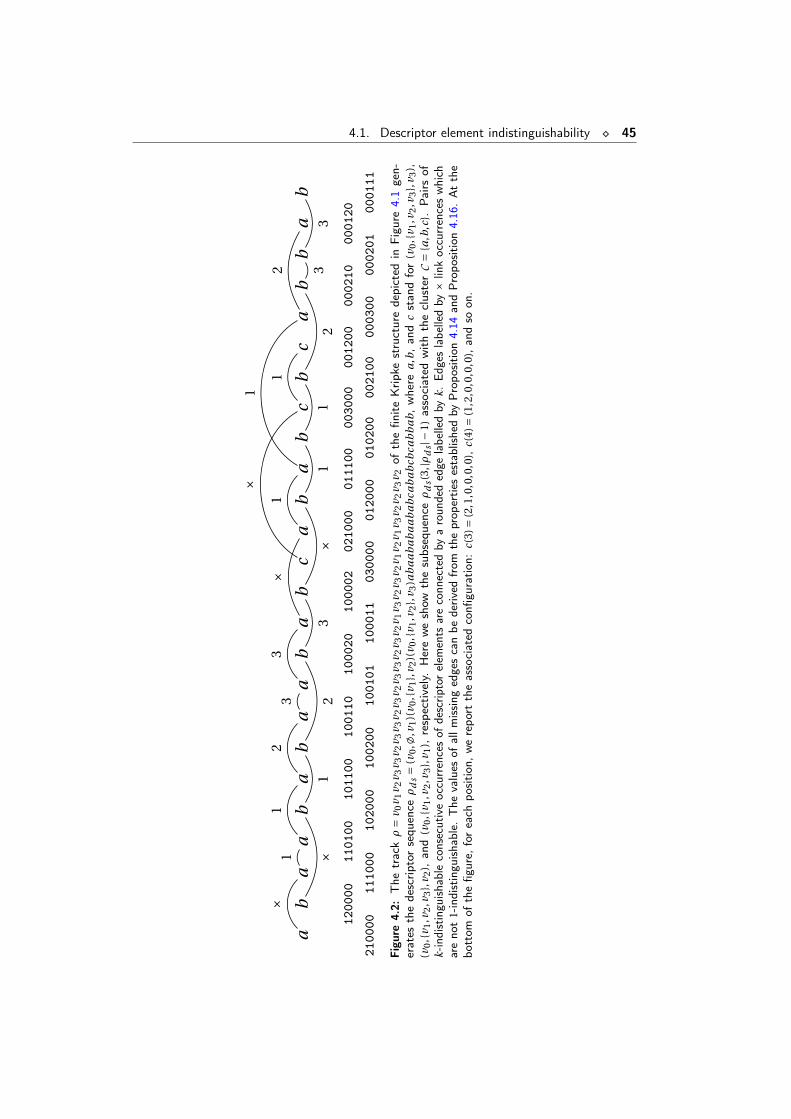
4.1. Descriptor element indistinguishability ¦ 45
ab
aa
ba
ba
ab
ab
ca
ba
bc
bc
ab
ba
b
×
×11
23
3
12
3
×
×
1
1
2
11
23
3
×1
2100
001200
00 1110
001101
00 1020
001011
00 1002
001001
10 1001
011000
20 1000
111000
02 0300
000210
00 0120
000111
00 0102
000030
00 0021
000012
00 0003
000002
10 0002
010001
20 0001
11
Figu
re4.
2:The
trackρ=
v 0v 1
v 2v 3
v 3v 2
v 3v 3
v 2v 3
v 2v 3
v 3v 2
v 3v 2
v 1v 3
v 2v 3
v 2v 1
v 2v 1
v 3v 2
v 2v 3
v 2of
thefin
iteKrip
kestructuredepicted
inFigu
re4.1gen-
erates
thedescrip
torsequ
ence
ρd
s=
(v0
,;,v
1)(
v 0,
v 1,
v 2)(
v 0,
v 1,v
2,
v 3)a
ba
ab
ab
aa
ba
bca
ba
bcb
cab
ba
b,where
a,b,and
cstandfor
(v0
,v 1
,v2
,v3
,v 3
),(v
0,
v 1,v
2,v
3,
v 2),and
(v0
,v 1
,v2
,v3
,v 1
),respectively.Hereweshow
thesubsequenceρ
ds(
3,|ρ
ds|−
1)associated
withthecluster
C=
a,b
,c.
Pairs
ofk-in
distingu
ishableconsecutiveoccurrencesof
descrip
torelem
ents
areconn
ectedby
aroun
dededge
labelledby
k.Ed
geslabelledby
×linkoccurrenceswhich
areno
t1-indistingu
ishable.
The
values
ofallm
issing
edgescanbe
deriv
edfrom
theprop
ertie
sestablishedby
Propo
sitio
n4.14
andPropo
sitio
n4.16
.Atthe
bottom
ofthefig
ure,
foreach
position
,werepo
rttheassociated
confi
guration
:c(
3)=
(2,1
,0,0
,0,0
),c(
4)=
(1,2
,0,0
,0,0
),andso
on.
46 ¦ Chapter 4. A model checking algorithm based on track representatives
such that d ∉ DEl m(ρd s (0, i − 1)), and the B1-descriptor for ρ(0, j + 1) has a leaflabeled by d which is not present in the B1-descriptor for ρ(0, i +1).
Inductive step (k ≥ 2). If ρd s (i ) and ρd s ( j ), with i < j , are not k-indistinguishable,then there exists (at least) one occurrence ρd s (i ′), with i ≤ i ′ < j , of a descriptorelement d which is not (k −1)-indistinguishable from any occurrence of d beforeposition i . By the inductive hypothesis, ρ(0, i ′+1) has a Bk−1-descriptor which is notisomorphic to any Bk−1-descriptor associated with proper prefixes of ρ(0, i +1). Thus,in the Bk -descriptor for ρ(0, j +1) there exists a subtree of depth k −1 such that thereis not an isomorphic subtree of depth k −1 in the Bk -descriptor for ρ(0, i +1).
Notice that k-indistinguishability between occurrences of descriptor elements isdefined only for pairs of prefixes of the same track, while the relation of k-descriptorequivalence can be applied to any pair of tracks of a Kripke structure.
We conclude the section with the following proposition, which easily follows fromTheorem 4.15.
Proposition 4.16. Let ρd s (i ), ρd s ( j ), and ρd s (m), with 0 ≤ i < j < m < |ρd s |, be threeoccurrences of the same descriptor element. If both the pair ρd s (i ) and ρd s ( j ) andthe pair ρd s ( j ) and ρd s (m) are k-indistinguishable, for some k ≥ 1, then ρd s (i ) andρd s (m) are k-indistinguishable as well.
4.2 Track representatives
In this section, we will exploit the k-indistinguishability relation between descriptorelements in a descriptor sequence ρd s for a track ρ to possibly replace ρ by a k-descriptor equivalent, shorter track ρ′ of bounded length. This allows us to find,for each (witnessed) Bk -descriptor DBk , a track representative ρ, witnessed in theconsidered finite Kripke structure, such that (i) DBk is the Bk -descriptor for ρ and(ii) the length of ρ is bounded. Thanks to property (ii), we can check all the trackrepresentatives of a finite Kripke structure by simply visiting its unravelling up to abounded depth.
The notion of track representative can be explained as follows. Let ρd s be thedescriptor sequence for a track ρ. If there exist two occurrences of the same descriptorelement ρd s (i ) and ρd s ( j ), with i < j , which are k-indistinguishable (we let ρ =ρ(0, j+1)·ρ andρ = ρ( j+2, |ρ|−1)), then we can replace the trackρ by the k-descriptorequivalent, shorter trackρ(0, i+1)·ρ. Indeed, by Theorem 4.15, ρ(0, i+1) andρ(0, j+1)have the same Bk -descriptor and thus, by Proposition 4.2, ρ = ρ(0, j + 1) ·ρ andρ(0, i + 1) ·ρ have the same Bk -descriptor. Moreover, since ρd s (i ) and ρd s ( j ) areoccurrences of the same descriptor element, ρ(i +1) = ρ( j +1) and thus the trackρ(0, i +1) ·ρ is witnessed in the finite Kripke structure. By iteratively applying sucha contraction method, we can find a track ρ′, which is k-descriptor equivalent to ρ,whose descriptor sequence is devoid of k-indistinguishable occurrences of descriptorelements. A track representative is a track that fulfils this property. In the rest of thesection, we shall consider the problem of establishing a bound to the length of trackrepresentatives.
We start by stating some technical properties. The next proposition providesa bound to the distance within which we observe a repeated occurrence of somedescriptor element in the descriptor sequence for a track. We preliminary observethat, for any track ρ, |DEl m(ρd s )| ≤ |W |2 +1, where W is the set of states of the finite
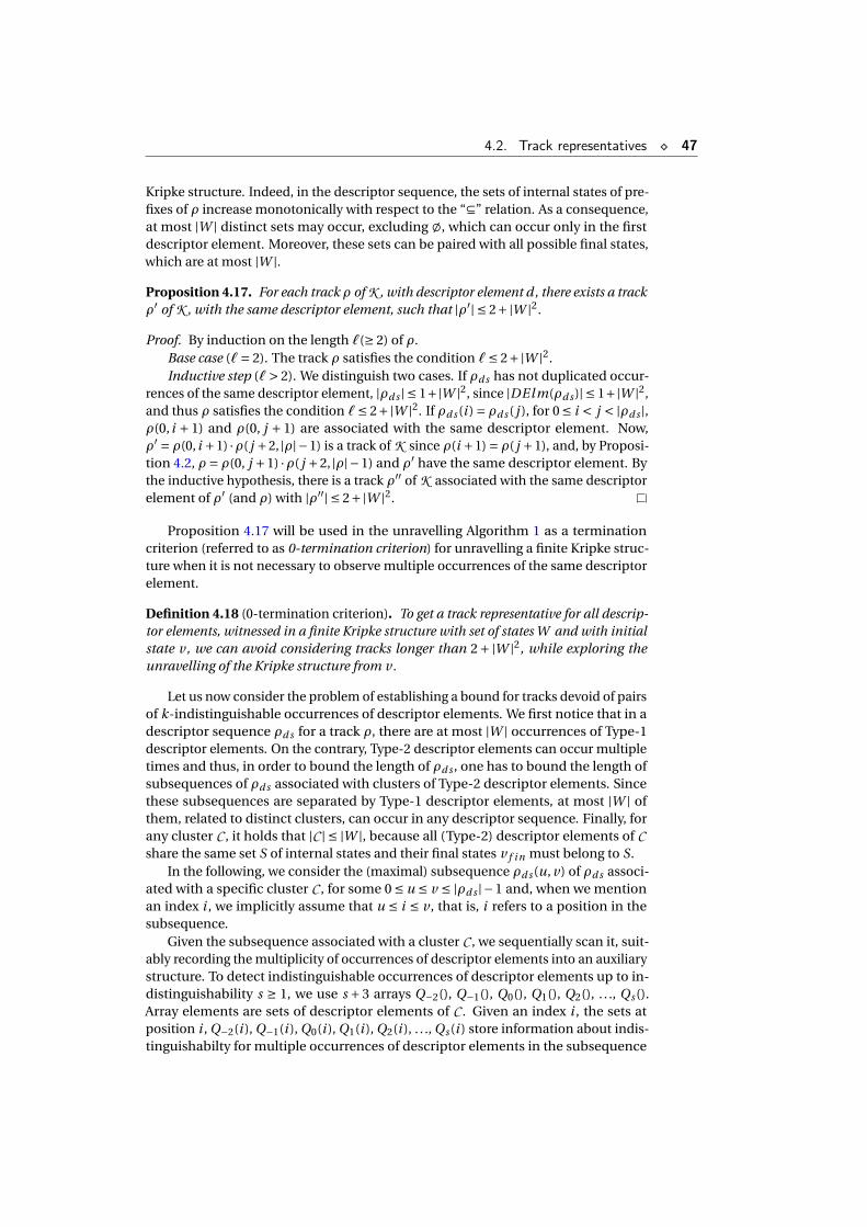
4.2. Track representatives ¦ 47
Kripke structure. Indeed, in the descriptor sequence, the sets of internal states of pre-fixes of ρ increase monotonically with respect to the “⊆” relation. As a consequence,at most |W | distinct sets may occur, excluding ;, which can occur only in the firstdescriptor element. Moreover, these sets can be paired with all possible final states,which are at most |W |.
Proposition 4.17. For each track ρ of K , with descriptor element d, there exists a trackρ′ of K , with the same descriptor element, such that |ρ′| ≤ 2+|W |2.
Proof. By induction on the length `(≥ 2) of ρ.Base case (`= 2). The track ρ satisfies the condition `≤ 2+|W |2.Inductive step (`> 2). We distinguish two cases. If ρd s has not duplicated occur-
rences of the same descriptor element, |ρd s | ≤ 1+|W |2, since |DElm(ρd s )| ≤ 1+|W |2,and thus ρ satisfies the condition `≤ 2+|W |2. If ρd s (i ) = ρd s ( j ), for 0 ≤ i < j < |ρd s |,ρ(0, i + 1) and ρ(0, j + 1) are associated with the same descriptor element. Now,ρ′ = ρ(0, i +1) ·ρ( j +2, |ρ|−1) is a track of K since ρ(i +1) = ρ( j +1), and, by Proposi-tion 4.2, ρ = ρ(0, j +1) ·ρ( j +2, |ρ|−1) and ρ′ have the same descriptor element. Bythe inductive hypothesis, there is a track ρ′′ of K associated with the same descriptorelement of ρ′ (and ρ) with |ρ′′| ≤ 2+|W |2.
Proposition 4.17 will be used in the unravelling Algorithm 1 as a terminationcriterion (referred to as 0-termination criterion) for unravelling a finite Kripke struc-ture when it is not necessary to observe multiple occurrences of the same descriptorelement.
Definition 4.18 (0-termination criterion). To get a track representative for all descrip-tor elements, witnessed in a finite Kripke structure with set of states W and with initialstate v, we can avoid considering tracks longer than 2+ |W |2, while exploring theunravelling of the Kripke structure from v.
Let us now consider the problem of establishing a bound for tracks devoid of pairsof k-indistinguishable occurrences of descriptor elements. We first notice that in adescriptor sequence ρd s for a track ρ, there are at most |W | occurrences of Type-1descriptor elements. On the contrary, Type-2 descriptor elements can occur multipletimes and thus, in order to bound the length of ρd s , one has to bound the length ofsubsequences of ρd s associated with clusters of Type-2 descriptor elements. Sincethese subsequences are separated by Type-1 descriptor elements, at most |W | ofthem, related to distinct clusters, can occur in any descriptor sequence. Finally, forany cluster C , it holds that |C | ≤ |W |, because all (Type-2) descriptor elements of Cshare the same set S of internal states and their final states v f i n must belong to S.
In the following, we consider the (maximal) subsequence ρd s (u, v) of ρd s associ-ated with a specific cluster C , for some 0 ≤ u ≤ v ≤ |ρd s |−1 and, when we mentionan index i , we implicitly assume that u ≤ i ≤ v , that is, i refers to a position in thesubsequence.
Given the subsequence associated with a cluster C , we sequentially scan it, suit-ably recording the multiplicity of occurrences of descriptor elements into an auxiliarystructure. To detect indistinguishable occurrences of descriptor elements up to in-distinguishability s ≥ 1, we use s + 3 arrays Q−2(), Q−1(), Q0(), Q1(), Q2(), . . ., Qs ().Array elements are sets of descriptor elements of C . Given an index i , the sets atposition i , Q−2(i ), Q−1(i ), Q0(i ), Q1(i ), Q2(i ), . . ., Qs (i ) store information about indis-tinguishabilty for multiple occurrences of descriptor elements in the subsequence
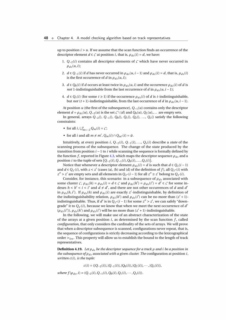
48 ¦ Chapter 4. A model checking algorithm based on track representatives
up to position i > u. If we assume that the scan function finds an occurrence of thedescriptor element d ∈ C at position i , that is, ρd s (i ) = d , we have:
1. Q−2(i ) contains all descriptor elements of C which have never occurred inρd s (u, i );
2. d ∈Q−1(i ) if d has never occurred in ρd s (u, i −1) and ρd s (i ) = d , that is, ρd s (i )is the first occurrence of d in ρd s (u, i );
3. d ∈Q0(i ) if d occurs at least twice in ρd s (u, i ) and the occurrence ρd s (i ) of d isnot 1-indistinguishable from the last occurrence of d in ρd s (u, i −1);
4. d ∈Qt (i ) (for some t ≥ 1) if the occurrence ρd s (i ) of d is t-indistinguishable,but not (t +1)-indistinguishable, from the last occurrence of d in ρd s (u, i −1).
At position u (the first of the subsequence), Q−1(u) contains only the descriptorelement d = ρd s (u), Q−2(u) is the set C \ d and Q0(u), Q1(u),. . . are empty sets.
In general, arrays Q−2(), Q−1(), Q0(), Q1(), Q2(), . . ., Qs () satisfy the followingconstraints:
• for all i ,⋃s
m=−2 Qm(i ) = C ;
• for all i and all m 6= m′, Qm(i )∩Qm′ (i ) =;.
Intuitively, at every position i , Q−2(i ), Q−1(i ), . . ., Qs (i ) describe a state of thescanning process of the subsequence. The change of the state produced by thetransition from position i −1 to i while scanning the sequence is formally defined bythe function f , reported in Figure 4.3, which maps the descriptor sequence ρd s and aposition i to the tuple of sets
(Q−2(i ),Q−1(i ),Q0(i ), . . . ,Qs (i )
).
Notice that whenever a descriptor element ρd s (i ) = d is such that d ∈Qz (i −1)and d ∈Qz ′ (i ), with z < z ′ (cases (a), (b) and (d) of the definition of f ), all Qz ′′ (i ) withz ′′ > z ′ are empty sets and all elements in Qz ′′ (i −1) for all z ′′ ≥ z ′ belong to Qz ′ (i ).
Consider, for instance, this scenario: in a subsequence of ρd s associated withsome cluster C , ρd s (h) = ρd s (i ) = d ∈ C and ρd s (h′) = ρd s (i ′) = d ′ ∈ C for some in-dexes h < h′ < i < i ′ and d 6= d ′, and there are not other occurrences of d and d ′in ρd s (h, i ′). If ρd s (h) and ρd s (i ) are exactly z ′-indistinguishable, by definition ofthe indistinguishability relation, ρd s (h′) and ρd s (i ′) can be no more than (z ′+1)-indistinguishable. Thus, if d ′ is in Qz ′′ (i −1) for some z ′′ > z ′, we can safely “down-grade” it to Qz ′ (i ), because we know that when we meet the next occurrence of d ′(ρd s (i ′)), ρd s (h′) and ρd s (i ′) will be no more than (z ′+1)-indistinguishable.
In the following, we will make use of an abstract characterization of the stateof the arrays at a given position i , as determined by the scan function f , calledconfiguration, that only considers the cardinality of the sets of arrays. We will provethat when a descriptor subsequence is scanned, configurations never repeat, that is,the sequence of configurations is strictly decreasing according to the lexicographicalorder >lex . This property will allow us to establish the bound to the length of trackrepresentatives.
Definition 4.19. Let ρd s be the descriptor sequence for a track ρ and i be a position inthe subsequence of ρd s associated with a given cluster. The configuration at position i ,written c(i ), is the tuple:
c(i ) = (|Q−2(i )|, |Q−1(i )|, |Q0(i )|, |Q1(i )|, · · · , |Qs (i )|),
where f (ρd s , i ) = (Q−2(i ),Q−1(i ),Q0(i ),Q1(i ), · · · ,Qs (i )).

4.2. Track representatives ¦ 49
f(ρ
ds,
u)=
( C\
d,
d,;,
···,;
) wit
hρ
ds(
u)=
d;
For
alli
>u
:f(ρ
ds,
i)=
( Q−2
(i),
Q−1
(i),
Q0
(i),
...,
Qs(
i)) =
( Q−2
(i−1
)\d
,d
∪⋃ s m
=−1
Qm
(i−1
),;,
...,;) if
ρd
s(i)
isth
efi
rsto
ccu
rren
ceo
fdinρ
ds(
u,i
);(a
)
( Q−2
(i−1
),Q
−1(i−1
)\d
,d
∪⋃ s m
=0Q
m(i−1
),;,
...,;) if
ρd
s(i)=
d,d
∈Q−1
(i−1
),an
dρ
ds(
i)is
atle
ast
the
seco
nd
occ
urr
ence
ofd
inρ
ds(
u,i
)an
dit
isn
ot1-
ind
isti
ngu
ish
able
fro
mth
eim
med
iate
lyp
rece
din
go
ccu
rren
ceo
fd;(
b)
( Q−2
(i−1
),Q
−1(i−1
),d
∪Q
0(i−1
),Q
1(i−1
)\d
,..
.,Q
s(i−1
)\d
) ifρ
ds(
i)=
d,d
∈⋃ s m=0
Qm
(i−1
),an
dρ
ds(
i)is
atle
ast
the
seco
nd
occ
urr
ence
ofd
inρ
ds(
u,i
)an
dit
isn
ot1-
ind
isti
ngu
ish
able
fro
mth
eim
med
iate
lyp
rece
din
go
ccu
rren
ceo
fd;(
c)
( Q−2
(i−1
)\d
,..
.,Q
t−1(i−1
)\d
,d
∪⋃ s m
=tQ
m(i−1
),;,
...,;) if
ρd
s(i)
=d
,ρ
ds(
i)is
t-in
dis
tin
guis
hab
le(f
or
som
et≥
1),
bu
tn
ot(t+1
)-in
dis
tin
guis
hab
le,t
oth
eim
med
iate
lyp
rece
din
go
ccu
rren
ceo
fd,a
nd
d∈⋃ t−
1m=−
2Q
m(i−1
);(d
)
( Q−2
(i−1
),···
,Qt−
1(i−1
),d
∪Q
t(i−
1),Q
t+1
(i−1
)\d
,..
.,Q
s(i−
1)\
d) if
ρd
s(i)=
d,ρ
ds(
i)is
t-in
dis
tin
guis
hab
le(f
or
som
et≥
1),b
ut
not
(t+1
)-in
dis
tin
guis
hab
le,t
oth
eim
med
iate
lyp
rece
din
go
ccu
rren
ceo
fd,a
nd
d∈⋃ s m
=tQ
m(i−1
).(e
)
Figu
re4.
3:Definition
ofthescan
function
f.
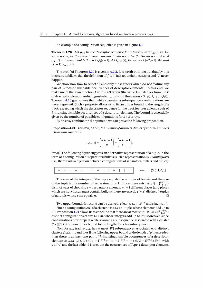
50 ¦ Chapter 4. A model checking algorithm based on track representatives
An example of a configuration sequence is given in Figure 4.2.
Theorem 4.20. Let ρd s be the descriptor sequence for a track ρ and ρd s (u, v), forsome u < v, be the subsequence associated with a cluster C . For all u < i ≤ v, ifρd s (i ) = d, then it holds that d ∈Qs (i −1), d ∈Qs+1(i ), for some s ∈ −2,−1∪N, andc(i −1) >lex c(i ).
The proof of Theorem 4.20 is given in A.2.2. It is worth pointing out that, by thistheorem, it follows that the definition of f is in fact redundant: cases (c) and (e) neverhappen.
We show now how to select all and only those tracks which do not feature anypair of k-indistinguishable occurrences of descriptor elements. To this end, wemake use of the scan function f with k +3 arrays (the value k +3 derives from the kof descriptor element indistinguishability, plus the three arrays Q−2(), Q−1(), Q0()).Theorem 4.20 guarantees that, while scanning a subsequence, configurations arenever repeated. Such a property allows us to fix an upper bound to the length of atrack, exceeding which the descriptor sequence for the track features at least a pair ofk-indistinguishable occurrences of a descriptor element. The bound is essentiallygiven by the number of possible configurations for k +3 arrays.
By an easy combinatorial argument, we can prove the following proposition.
Proposition 4.21. For all n, t ∈N+, the number of distinct t-tuples of natural numberswhose sum equals n is
ε(n, t ) =(
n + t −1
n
)=
(n + t −1
t −1
).
Proof. The following figure suggests an alternative representation of a tuple, in theform of a configuration of separators/bullets; such a representation is unambiguous(i.e., there exists a bijection between configurations of separators/bullets and tuples):
| | | | ! (5,3,1,0,1)
The sum of the integers of the tuple equals the number of bullets and the sizeof the tuple is the number of separators plus 1. Since there exist ε(n, t) = (n+t−1
t−1
)distinct ways of choosing t −1 separators among n+ t −1 different places (and placeswhich are not chosen must contain bullets), there are exactly ε(n, t ) distinct t-tuplesof naturals whose sum equals n.
Two upper bounds for ε(n, t ) can be derived: ε(n, t ) ≤ (n +1)t−1 and ε(n, t ) ≤ t n .Since a configuration c(i ) of a cluster C is a (k+3)-tuple, whose elements add up to
|C |, Proposition 4.21 allows us to conclude that there are at most ε(|C |,k+3) = (|C |+k+2k+2
)distinct configurations of size (k +3), whose integers add up to |C |. Moreover, sinceconfigurations never repeat while scanning a subsequence associated with a clusterC , ε(|C |,k +3) is an upper bound to the length of such a subsequence.
Now, for any track ρ, ρd s has at most |W | subsequences associated with distinctclusters C1,C2, . . . , and thus if the following upper bound to the length of ρ is exceeded,then there is at least one pair of k-indistinguishable occurrences of a descriptorelement in ρd s : |ρ| ≤ 1+ (|C1| + 1)k+2 + (|C2| + 1)k+2 + ·· · + (|Cs | + 1)k+2 + |W |, withs ≤ |W | and the last addend is to count the occurrences of Type-1 descriptor elements.
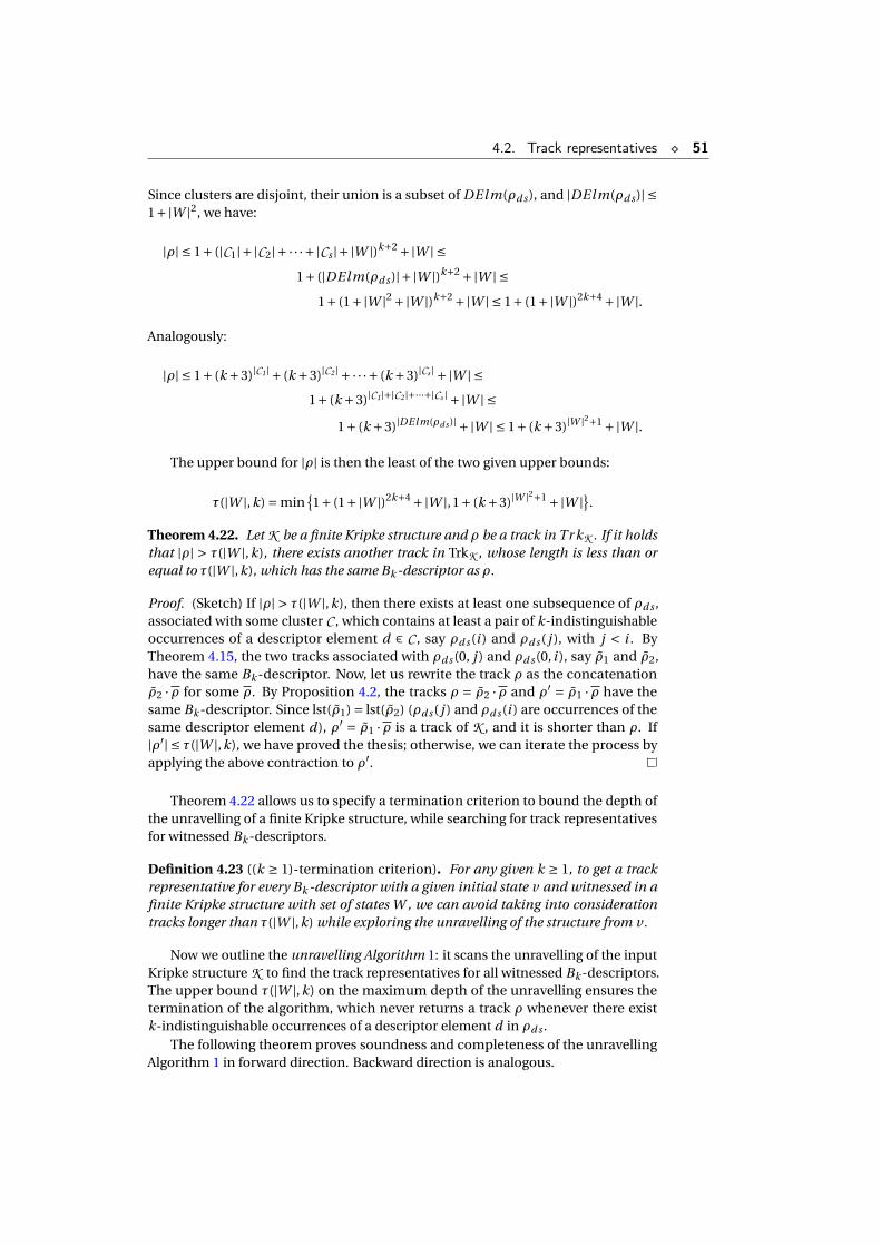
4.2. Track representatives ¦ 51
Since clusters are disjoint, their union is a subset of DEl m(ρd s ), and |DElm(ρd s )| ≤1+|W |2, we have:
|ρ| ≤ 1+ (|C1|+ |C2|+ · · ·+ |Cs |+ |W |)k+2 +|W | ≤1+ (|DElm(ρd s )|+ |W |)k+2 +|W | ≤
1+ (1+|W |2 +|W |)k+2 +|W | ≤ 1+ (1+|W |)2k+4 +|W |.
Analogously:
|ρ| ≤ 1+ (k +3)|C1|+ (k +3)|C2 |+·· ·+ (k +3)|Cs |+|W | ≤1+ (k +3)|C1|+|C2 |+···+|Cs |+|W | ≤
1+ (k +3)|DEl m(ρd s )|+|W | ≤ 1+ (k +3)|W |2+1 +|W |.
The upper bound for |ρ| is then the least of the two given upper bounds:
τ(|W |,k) = min1+ (1+|W |)2k+4 +|W |,1+ (k +3)|W |2+1 +|W |.
Theorem 4.22. Let K be a finite Kripke structure and ρ be a track in Tr kK . If it holdsthat |ρ| > τ(|W |,k), there exists another track in TrkK , whose length is less than orequal to τ(|W |,k), which has the same Bk -descriptor as ρ.
Proof. (Sketch) If |ρ| > τ(|W |,k), then there exists at least one subsequence of ρd s ,associated with some cluster C , which contains at least a pair of k-indistinguishableoccurrences of a descriptor element d ∈ C , say ρd s (i ) and ρd s ( j ), with j < i . ByTheorem 4.15, the two tracks associated with ρd s (0, j ) and ρd s (0, i ), say ρ1 and ρ2,have the same Bk -descriptor. Now, let us rewrite the track ρ as the concatenationρ2 ·ρ for some ρ. By Proposition 4.2, the tracks ρ = ρ2 ·ρ and ρ′ = ρ1 ·ρ have thesame Bk -descriptor. Since lst(ρ1) = lst(ρ2) (ρd s ( j ) and ρd s (i ) are occurrences of thesame descriptor element d), ρ′ = ρ1 ·ρ is a track of K , and it is shorter than ρ. If|ρ′| ≤ τ(|W |,k), we have proved the thesis; otherwise, we can iterate the process byapplying the above contraction to ρ′.
Theorem 4.22 allows us to specify a termination criterion to bound the depth ofthe unravelling of a finite Kripke structure, while searching for track representativesfor witnessed Bk -descriptors.
Definition 4.23 ((k ≥ 1)-termination criterion). For any given k ≥ 1, to get a trackrepresentative for every Bk -descriptor with a given initial state v and witnessed in afinite Kripke structure with set of states W , we can avoid taking into considerationtracks longer than τ(|W |,k) while exploring the unravelling of the structure from v.
Now we outline the unravelling Algorithm 1: it scans the unravelling of the inputKripke structure K to find the track representatives for all witnessed Bk -descriptors.The upper bound τ(|W |,k) on the maximum depth of the unravelling ensures thetermination of the algorithm, which never returns a track ρ whenever there existk-indistinguishable occurrences of a descriptor element d in ρd s .
The following theorem proves soundness and completeness of the unravellingAlgorithm 1 in forward direction. Backward direction is analogous.

52 ¦ Chapter 4. A model checking algorithm based on track representatives
Algorithm 1 Unrav(K , v,k,direction)1: / “¿” is an arbitrary order of the nodes of K2: if direction = FORWARD then3: Unravel K starting from v according to ¿4: For every new node of the unravelling met during the visit, return the track ρ from v to the current
node only if:5: if k = 0 then6: Apply 0-termination criterion of Definition 4.187: else8: if The last descriptor element d of (the descriptor sequence of) the current track ρ is k-
indistinguishable from a previous occurrence of d then9: do not return ρ and backtrack to ρ(0, |ρ|−2) · v , where v is the minimum state (w.r.t. ¿)
greater than ρ(|ρ|−1) such that (ρ(|ρ|−2), v) is an edge of K .
10: else if direction = BACKWARD then11: Unravel K starting from v according to ¿ / K is K with transposed edges12: For every new node of the unravelling met during the visit, consider the track ρ from the current
node to v , and recalculate descriptor elements indistinguishability from scratch (left to right); returnthe track only if:
13: if k = 0 then14: Apply 0-termination criterion of Definition 4.1815: else16: if There exist two k-indistinguishable occurrences of a descriptor element d in (the descriptor
sequence of) the current track ρ then17: do not return ρ
18: Do not visit tracks of length greater than τ(|W |,k)
Theorem 4.24. Let K be a finite Kripke structure, v be a state in W , and k ∈N. Forevery track ρ of K , with fst(ρ) = v and |ρ| ≥ 2, the unravelling algorithm returns atrack ρ′ of K , with fst(ρ′) = v, such that ρ and ρ′ have the same Bk -descriptor and|ρ′| ≤ τ(|W |,k).
The proof of Theorem 4.24 is given in A.2.3. It basically shows how a “contractedvariant” of a track ρ is (indirectly) computed by Algorithm 1.
As an example, in place of the track ρ of Figure 4.2, the algorithm returns the fol-lowing contracted track: ρ′ = v0v1v2v3v3v2v3v3v2v3v2v3v2v1v3v2v3v2v1v2v1v3v2.It can be checked that ρ′ does not contain any pair of 3-indistinguishable occurrencesof a descriptor element and that ρ and ρ′ have the same B3-descriptor.
In the forward modality, the direction of track exploration and that of indistin-guishability checking are the same, so we can stop extending a track as soon as thefirst pair of k-indistinguishable occurrences of a descriptor element is found in thedescriptor sequence, suggesting an easy termination criterion for stopping the unrav-elling of tracks. In the backward modality, such a straightforward criterion cannotbe adopted, because tracks are explored right to left (the opposite direction withrespect to edges of the Kripke structure), while the indistinguishability relation overoccurrences of descriptor elements is computed left to right. In general, changingthe prefix of a considered track requires recomputing from scratch the descriptorsequence and the indistinguishability relation over descriptor elements. In particular,k-indistinguishable occurrences of descriptor elements can be detected in the middleof a subsequence, and not necessarily at the end.
Luckily, a heuristic is applicable when dealing with the backward modality: ifthe descriptor sequence ρd s for ρ contains a pair of k-indistinguishable occurrencesρd s ( j ) and ρd s (i ) of the same descriptor element, with j < i , it is possible to skipthe exploration of tracks of the form ρ ·ρ, for any ρ ∈ TrkK . Since ρ(0, j + 1) andρ(0, i +1) have the same Bk -descriptor, by Proposition 4.3 for any ρ ∈ TrkK such that
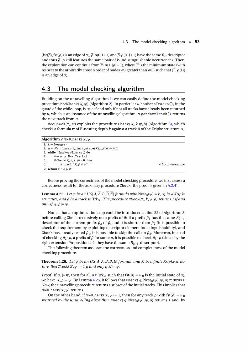
4.3. The model checking algorithm ¦ 53
(lst(ρ), fst(ρ)) is an edge of K , ρ·ρ(0, i+1) andρ·ρ(0, j+1) have the same Bk -descriptorand thus ρ ·ρ still features the same pair of k-indistinguishable occurrences. Then,the exploration can continue from v ·ρ(1, |ρ|−1), where v is the minimum state (withrespect to the arbitrarily chosen order of nodes ¿) greater than ρ(0) such that (v ,ρ(1))is an edge of K .
4.3 The model checking algorithm
Building on the unravelling Algorithm 1, we can easily define the model checkingprocedure ModCheck(K ,ψ) (Algorithm 2). In particular u.hasMoreTracks(), in theguard of the while-loop, is true if and only if not all tracks have already been returnedby u, which is an instance of the unravelling algorithm; u.getNextTrack() returnsthe next track from u.
ModCheck(K ,ψ) exploits the procedure Check(K ,k,ψ, ρ) (Algorithm 3), whichchecks a formula ψ of B-nesting depth k against a track ρ of the Kripke structure K .
Algorithm 2 ModCheck(K ,ψ)1: k ← NestB(ψ)2: u ← New (Unrav(K ,init_state(K ),k, FORWARD))3: while u.hasMoreTracks() do4: ρ← u.getNextTrack()5: if Check(K ,k,ψ, ρ) = 0 then6: return 0: “K , ρ 6|=ψ” / Counterexample
7: return 1: “K |=ψ”
Before proving the correctness of the model checking procedure, we first assess acorrectness result for the auxiliary procedure Check (the proof is given in A.2.4).
Lemma 4.25. Let ψ be an HS[A, A,B ,B ,E ] formula with NestB(ψ) = k, K be a Kripkestructure, and ρ be a track in TrkK . The procedure Check(K ,k,ψ, ρ) returns 1 if andonly if K , ρ |=ψ.
Notice that an optimization step could be introduced at line 32 of Algorithm 3,before calling Check recursively on a prefix of ρ: if a prefix ρ1 has the same Bk−1-descriptor of the current prefix ρ2 of ρ, and it is shorter than ρ2 (it is possible tocheck the requirement by exploiting descriptor element indistinguishability), andCheck has already tested ρ1, it is possible to skip the call on ρ2. Moreover, insteadof checking ρ2 ·ρ, a prefix of ρ for some ρ, it is possible to check ρ1 ·ρ (since, by theright extension Proposition 4.2, they have the same Bk−1-descriptor).
The following theorem assesses the correctness and completeness of the modelchecking procedure.
Theorem 4.26. Let ψ be an HS[A, A,B ,B ,E ] formula and K be a finite Kripke struc-ture. ModCheck(K ,ψ) = 1 if and only if K |=ψ.
Proof. If K |=ψ, then for all ρ ∈ TrkK such that fst(ρ) = w0 is the initial state of K ,we have K ,ρ |=ψ. By Lemma 4.25, it follows that Check(K ,NestB(ψ),ψ,ρ) returns 1.Now, the unravelling procedure returns a subset of the initial tracks. This implies thatModCheck(K ,ψ) returns 1.
On the other hand, if ModCheck(K ,ψ) = 1, then for any track ρ with fst(ρ) = w0
returned by the unravelling algorithm, Check(K ,NestB(ψ),ψ,ρ) returns 1 and, by
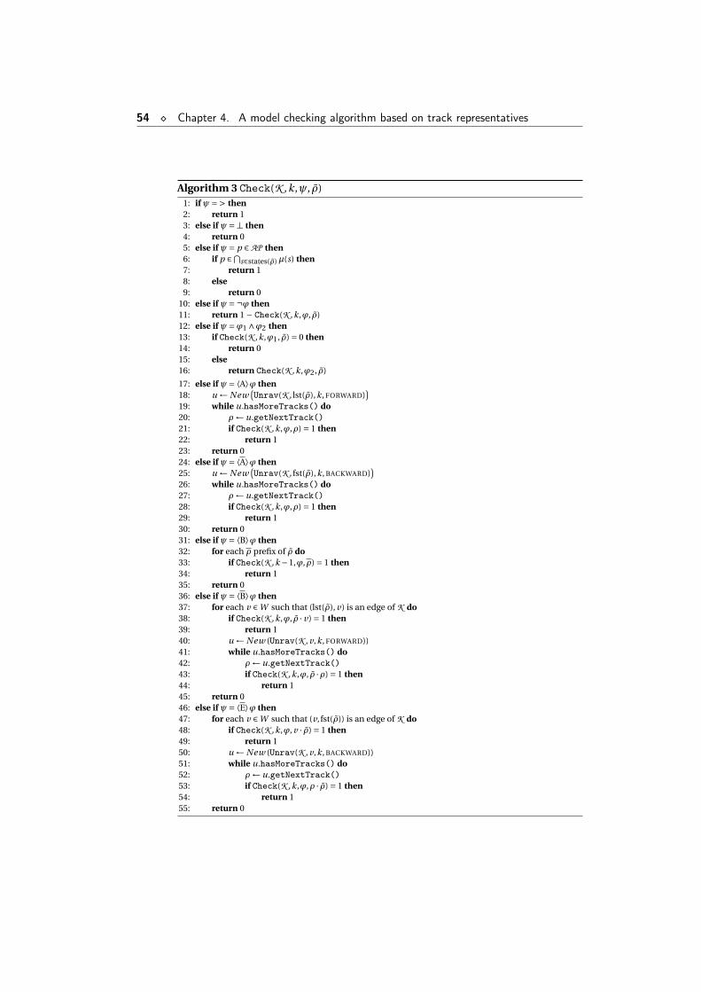
54 ¦ Chapter 4. A model checking algorithm based on track representatives
Algorithm 3 Check(K ,k,ψ, ρ)1: if ψ=> then2: return 13: else if ψ=⊥ then4: return 05: else if ψ= p ∈ AP then6: if p ∈⋂
s∈states(ρ)µ(s) then7: return 18: else9: return 0
10: else if ψ=¬ϕ then11: return 1 − Check(K ,k,ϕ, ρ)12: else if ψ=ϕ1 ∧ϕ2 then13: if Check(K ,k,ϕ1, ρ) = 0 then14: return 015: else16: return Check(K ,k,ϕ2, ρ)
17: else if ψ= ⟨A⟩ϕ then18: u ← New
(Unrav(K , lst(ρ),k, FORWARD)
)19: while u.hasMoreTracks() do20: ρ← u.getNextTrack()21: if Check(K ,k,ϕ,ρ) = 1 then22: return 123: return 024: else if ψ= ⟨A⟩ϕ then25: u ← New
(Unrav(K , fst(ρ),k, BACKWARD)
)26: while u.hasMoreTracks() do27: ρ← u.getNextTrack()28: if Check(K ,k,ϕ,ρ) = 1 then29: return 130: return 031: else if ψ= ⟨B⟩ϕ then32: for each ρ prefix of ρ do33: if Check(K ,k −1,ϕ,ρ) = 1 then34: return 135: return 036: else if ψ= ⟨B⟩ϕ then37: for each v ∈W such that (lst(ρ), v) is an edge of K do38: if Check(K ,k,ϕ, ρ · v) = 1 then39: return 140: u ← New (Unrav(K , v,k, FORWARD))41: while u.hasMoreTracks() do42: ρ← u.getNextTrack()43: if Check(K ,k,ϕ, ρ ·ρ) = 1 then44: return 145: return 046: else if ψ= ⟨E⟩ϕ then47: for each v ∈W such that (v, fst(ρ)) is an edge of K do48: if Check(K ,k,ϕ, v · ρ) = 1 then49: return 150: u ← New (Unrav(K , v,k, BACKWARD))51: while u.hasMoreTracks() do52: ρ← u.getNextTrack()53: if Check(K ,k,ϕ,ρ · ρ) = 1 then54: return 155: return 0
4.4. NEXP-hardness of model checking for HS[A, A,B ,B ,E ] ¦ 55
Lemma 4.25, we have K ,ρ |=ψ. Assume now that a track ρ with fst(ρ) = w0 is notreturned by the unravelling algorithm. By Theorem 4.24, there is a track ρ, withfst(ρ) = w0, which is returned in place of ρ and ρ has the same Bk -descriptor as ρ(with k = NestB(ψ)). Since K , ρ |=ψ ⇐⇒ K ,ρ |=ψ (by Theorem 4.4) and K ,ρ |=ψ,we get that K , ρ |=ψ. So all tracks starting with state w0 model ψ, thus K |=ψ.
Finally, we observe that the model checking algorithm ModCheck is in EXPSPACE.Indeed, ModCheck uses an instance of the unravelling algorithm and some additionalspace for a track ρ. Analogously, every recursive call to Check needs an instance ofthe unravelling algorithm and space for a track. Since there are at most |ψ| (whereψ is the input formula) simultaneously active calls to Check, the total space neededby the considered algorithms is
(|ψ|+1) ·O(|W | +NestB(ψ)) ·τ(|W |,NestB(ψ)) bits
overall, where τ(|W |,NestB(ψ)) is the maximum length of track representatives, andO(|W | +NestB(ψ)) bits are needed to represent a state of K , a descriptor element,and a counter for k-indistinguishability.
As a particular case, formulas ψ of the fragment HS[A, A,B ,E ] can be checkedin polynomial space, because for these formulas NestB(ψ) = 0 (we will come back tothis HS fragment in the next chapter).
4.4 NEXP-hardness of model checking for thefragment HS[A, A,B ,B ,E ]
We conclude this chapter by proving that the model checking problem for formulas ofthe fragment HS[A, A,B ,B ,E ], interpreted over finite Kripke structures, is NEXP-hardwhen a succinct encoding of formulas is exploited (Theorem 4.27). Like in the proofof Theorem 3.12, we allow to write ⟨B⟩k ψ standing for k repetitions of ⟨B⟩ beforeψ, with k represented in binary. The same can be done for all other HS modalities.Additionally,
∧i=l ,··· ,r ψ(i ) denotes a conjunction of formulas which contain some
occurrences of the index i as exponents (l and r are binary encoded naturals), forexample
∧i=1,··· ,5 ⟨B⟩i >.
We finally denote by expand(ψ) the expanded form of ψ: all exponents k haveto be eliminated from ψ by explicitly repeating k times each HS modality with suchan exponent, and big conjunctions must be replaced by conjunctions of formulaswithout indexes.
Theorem 4.27. The model checking problem for succinct HS[A, A,B ,B ,E ] formulasagainst finite Kripke structures is NEXP-hard.
Proof. Since this proof is very similar to that of Theorem 3.12, we only outline whichelements have to be changed.
• We consider a language L decided by a non-deterministic one-tape Turing
machine M (w.l.o.g.) that halts after no more than 2nk −3 computation stepson an input of size n (L belongs to NEXP).
• As a consequence, M uses at most 2nk −3 cells on its tape, so the size of a con-
figuration is 2nk. Moreover the number of configurations is 2nk −3. Therefore
the computation table is now a matrix of 2nk −3 rows and 2nkcolumns.
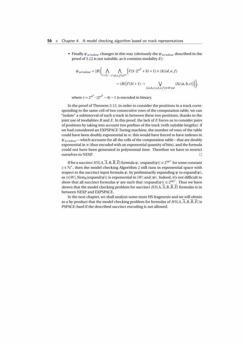
56 ¦ Chapter 4. A model checking algorithm based on track representatives
• Finally ψwi ndow changes in this way (obviously the ψwi ndow described in theproof of 3.12 is not suitable, as it contains modality E):
ψwi ndow = [B ]
( ∧i=2,··· ,t
∧(d ,e, f )∈Γ3
(`(3 ·2nk +3i +1)∧⟨A⟩(d ,e, f )
→ [B ](`(3i +1) → ∨
((a,b,c),(d ,e, f ))∈W nd⟨A⟩(a,b,c)
))),
where t = 2nk · (2nk −4)−1 is encoded in binary.
In the proof of Theorem 3.12, in order to consider the positions in a track corre-sponding to the same cell of two consecutive rows of the computation table, we can“isolate” a subinterval of such a track in between these two positions, thanks to thejoint use of modalities B and E . In this proof, the lack of E forces us to consider pairsof positions by taking into account two prefixes of the track (with suitable lengths): ifwe had considered an EXPSPACE Turing machine, the number of rows of the tablecould have been doubly exponential in n: this would have forced to have indexes inψwi ndow —which accounts for all the cells of the computation table—that are doublyexponential in n (thus encoded with an exponential quantity of bits), and the formulacould not have been generated in polynomial time. Therefore we have to restrictourselves to NEXP.
If for a succinct HS[A, A,B ,B ,E ] formulaψ, |expand(ψ)| ≤ 2|ψ|c for some constantc ∈ N+, then the model checking Algorithm 2 still runs in exponential space withrespect to the succinct input formula ψ, by preliminarily expanding ψ to expand(ψ),as τ(|W |,NestB(expand(ψ)) is exponential in |W | and |ψ|. Indeed, it’s not difficult toshow that all succinct formulas ψ are such that |expand(ψ)| ≤ 2|ψ|c . Thus we haveshown that the model checking problem for succinct HS[A, A,B ,B ,E ] formulas is inbetween NEXP and EXPSPACE.
In the next chapter, we shall analyze some more HS fragments and we will obtainas a by-product that the model checking problem for formulas of HS[A, A,B ,B ,E ] isPSPACE-hard if the described succinct encoding is not allowed.
5Some well-behaved fragments
of HS
Contents5.1 The fragments ∀HS[A, A,B ,E ], HS[A, A], and HS[Prop] . . . . . . 595.2 The fragment HS[A, A,B ,E ] . . . . . . . . . . . . . . . . . . . . . . . 64
In this chapter, we identify some well-behaved fragments of the HS logic, namely,∀HS[A, A,B ,E ] (and ∃HS[A, A,B ,E ]), HS[A, A,B ,E ], and HS[A, A], which are still ex-pressive enough to capture meaningful interval properties of state-transition systemsand whose model checking problem exhibits a considerably lower computationalcomplexity.
In Section 5.1, we deal with the fragment ∀HS[A, A,B ,E ], including formulasof HS[A, A,B ,E ] in which only universal modalities are allowed and negation canbe applied to propositional formulas only. We first provide a coNP model checkingalgorithm for ∀HS[A, A,B ,E ], and then we show that the model checking problemfor the pure propositional fragment HS[Prop] is coNP-hard. The two results allow usto conclude that the model checking problem for both HS[Prop] and ∀HS[A, A,B ,E ]is coNP-complete. In addition, upper and lower bounds to the complexity of theproblem for HS[A, A] (the logic of temporal neighbourhood) directly follow. Recallthat the model checking algorithm for HS[A, A,B ,B ,E ] of Section 4.3 can checkformulas of HS[A, A,B ,E ] in polynomial space. Since HS[A, A] is a fragment ofHS[A, A,B ,E ] and HS[Prop] is a fragment of HS[A, A], complexity of model checkingfor HS[A, A] is in between coNP and PSPACE.
In Section 5.2, we focus our attention on HS[A, A,B ,E ] and we prove that themodel checking problem for HS[A,B ] is PSPACE-hard. PSPACE-completeness ofHS[A, A,B ,E ] (and HS[A,B ]) immediately follows. From this, we get for free a lowerbound to the complexity of the model checking problem for HS[A, A,B ,B ,E ] in thenon-succinct case, which turns out to be PSPACE-hard.
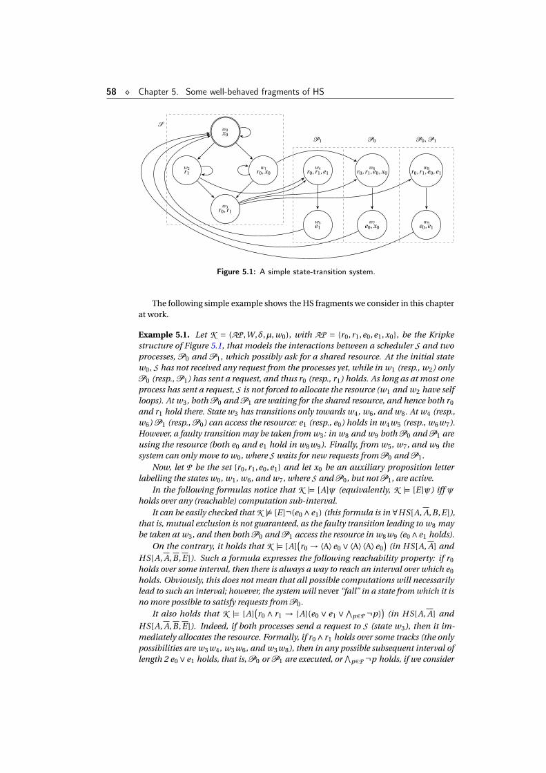
58 ¦ Chapter 5. Some well-behaved fragments of HS
w0x0
w1r0, x0
w2r1
w3r0,r1
w4r0,r1,e1
w5e1
w6r0,r1,e0, x0
w7e0, x0
w8r0,r1,e0,e1
w9e0,e1
P1 P0 P0, P1
S
Figure 5.1: A simple state-transition system.
The following simple example shows the HS fragments we consider in this chapterat work.
Example 5.1. Let K = (AP ,W,δ,µ, w0), with AP = r0,r1,e0,e1, x0, be the Kripkestructure of Figure 5.1, that models the interactions between a scheduler S and twoprocesses, P0 and P1, which possibly ask for a shared resource. At the initial statew0, S has not received any request from the processes yet, while in w1 (resp., w2) onlyP0 (resp., P1) has sent a request, and thus r0 (resp., r1) holds. As long as at most oneprocess has sent a request, S is not forced to allocate the resource (w1 and w2 have selfloops). At w3, both P0 and P1 are waiting for the shared resource, and hence both r0
and r1 hold there. State w3 has transitions only towards w4, w6, and w8. At w4 (resp.,w6) P1 (resp., P0) can access the resource: e1 (resp., e0) holds in w4w5 (resp., w6w7).However, a faulty transition may be taken from w3: in w8 and w9 both P0 and P1 areusing the resource (both e0 and e1 hold in w8w9). Finally, from w5, w7, and w9 thesystem can only move to w0, where S waits for new requests from P0 and P1.
Now, let P be the set r0,r1,e0,e1 and let x0 be an auxiliary proposition letterlabelling the states w0, w1, w6, and w7, where S and P0, but not P1, are active.
In the following formulas notice that K |= [A]ψ (equivalently, K |= [E ]ψ) iff ψholds over any (reachable) computation sub-interval.
It can be easily checked that K 6|= [E ]¬(e0 ∧e1) (this formula is in ∀HS[A, A,B ,E ]),that is, mutual exclusion is not guaranteed, as the faulty transition leading to w8 maybe taken at w3, and then both P0 and P1 access the resource in w8w9 (e0 ∧e1 holds).
On the contrary, it holds that K |= [A](r0 → ⟨A⟩e0 ∨⟨A⟩⟨A⟩e0
)(in HS[A, A] and
HS[A, A,B ,E ]). Such a formula expresses the following reachability property: if r0
holds over some interval, then there is always a way to reach an interval over which e0
holds. Obviously, this does not mean that all possible computations will necessarilylead to such an interval; however, the system will never “fall” in a state from which it isno more possible to satisfy requests from P0.
It also holds that K |= [A](r0 ∧ r1 → [A](e0 ∨ e1 ∨∧
p∈P ¬p))
(in HS[A, A] and
HS[A, A,B ,E ]). Indeed, if both processes send a request to S (state w3), then it im-mediately allocates the resource. Formally, if r0 ∧ r1 holds over some tracks (the onlypossibilities are w3w4, w3w6, and w3w8), then in any possible subsequent interval oflength 2 e0 ∨e1 holds, that is, P0 or P1 are executed, or
∧p∈P ¬p holds, if we consider
5.1. The fragments ∀HS[A, A,B ,E ], HS[A, A], and HS[Prop] ¦ 59
tracks longer than 2. On the contrary, if only one process asks for the resource, then Scan arbitrarily delay its allocation, that is, K 6|= [A]
(r0 → [A](e0 ∨∧
p∈P ¬p)).
Finally, it holds that K |= x0 →⟨B⟩x0 (in HS[A, A,B ,E ]), that is, any initial tracksatisfying x0 (any such track features occurrences of states w0, w1, w6, and w7 only)can be extended to the right in such a way that the resulting track still satisfies x0. Thisamounts to say that there exists a computation in which P1 starves. Notice that S andP0 can continuously interact without waiting for P1. This is the case, for instance,when P1 does not ask for the shared resource at all.
5.1 The fragments ∀HS[A, A,B ,E ], HS[A, A], andHS[Prop]
In this section, we take into consideration the universal and existential fragmentsof HS[A, A,B ,E ], respectively denoted by ∀HS[A, A,B ,E ] and ∃HS[A, A,B ,E ], whoseformulas are defined as follows:
ψ ::=β |ψ∧ψ | [A]ψ | [B ]ψ | [E ]ψ | [A]ψ
(resp., ψ ::=β |ψ∨ψ | ⟨A⟩ψ | ⟨B⟩ψ | ⟨E⟩ψ | ⟨A⟩ψ),
whereβ ::= p |β∨β |β∧β | ¬β | ⊥ | > with p ∈ AP .
The intersection of ∀HS[A, A,B ,E ] and ∃HS[A, A,B ,E ] is the set of all and onlypure propositional formulas (HS[Prop]). Negations occur in pure propositional for-mulas only, and formulas with modalities can be combined only by conjunctions (in∀HS[A, A,B ,E ]) or disjunctions (in ∃HS[A, A,B ,E ]). The negation of any formula of∀HS[A, A,B ,E ] can be transformed into an equivalent ∃HS[A, A,B ,E ] formula (of atmost double length), and vice versa, by using De Morgan’s laws and the equivalences[X ]ψ≡¬⟨X ⟩¬ψ and ¬¬ψ≡ψ.
We now outline a non-deterministic algorithm to decide the model checking prob-lem for a ∀HS[A, A,B ,E ] formula ψ. The algorithm searches for a counterexample toψ. As we already pointed out, ¬ψ is equivalent to a suitable formula ψ′ of the dualfragment ∃HS[A, A,B ,E ]. Hence, the algorithm looks for an initial track of the Kripkestructure that satisfies ψ′.
For the satisfiability check, we use the non-deterministic procedure Check (Algo-rithm 4), which does not exploit (directly or indirectly) neither BEk - descriptors norBk -descriptors, but only descriptor elements.
Recall that (Proposition 4.17, Definition 4.18) if a descriptor element d is wit-nessed, then there exists a track of length at most 2+|W |2 associated with it, and thusto generate a (all) witnessed descriptor element(s) with initial state v , we just need tonon-deterministically visit the unravelling of K from v up to depth 2+|W |2.
The procedure Check takes as input a formula ψ of ∃HS[A, A,B ,E ] and a wit-nessed descriptor element d = (vi n ,S, v f i n) and it returns Yes if and only if thereexists a track ρ ∈ TrkK associated with d such that K ,ρ |=ψ. The procedure is recur-sively defined as follows.
If it is called on a Boolean combination β of proposition letters (base of therecursion), V AL(β,d) evaluates β over d in the standard way. The evaluation can beperformed in deterministic polynomial time, and if V AL(β,d) returns >, then thereexists a track associated with d (of length at most quadratic in |W |) that satisfies β.
60 ¦ Chapter 5. Some well-behaved fragments of HS
If ψ has the form ψ′∨ψ′′, the procedure non-determistically calls itself on ψ′ orψ′′ (the control construct Either c1 Or c2 EndOr denotes a non-deterministic choicebetween commands c1 and c2).
If ψ has the form ⟨A⟩ψ′ (resp., ⟨A⟩ψ′), the procedure looks for a new descriptorelement for a track starting from the final state (resp., leading to the initial state) of thecurrent descriptor element d . To this end, we use the procedure aDescrEl(K , v, FORW)(resp., aDescrEl(K , v, BACKW)) which non-deterministically returns a descriptor ele-ment (v ′
i n ,S′, v ′f i n), with v ′
i n = v (resp., v ′f i n = v), witnessed in K by exploring forward
(resp., backward) the unravelling of K from v ′i n (resp., from v ′
f i n). Its complexity is
polynomial in |W |, since it needs to examine the unravelling of K from v up to depth2+|W |2.
If ψ has the form ⟨B⟩ψ′, the procedure looks for a new descriptor element d1 andeventually calls itself onψ′ and d1 only if the current descriptor element d results fromthe “concatenation” of d1 with a suitable descriptor element d2: if d1 = (v ′
i n ,S′, v ′f i n)
and d2 = (v ′′i n ,S′′, v ′′
f i n), then concat(d1,d2) returns the descriptor element (v ′i n ,S′∪
v ′f i n , v ′′
i n∪S′′, v ′′f i n). Notice that if ρ1 and ρ2 are tracks associated with d1 and d2,
respectively, then ρ1 ·ρ2 is associated with concat(d1,d2).The following theorem proves soundness and completeness of the Check proce-
dure.
Theorem 5.2. For any ∃HS[A, A,B ,E ] formula ψ and any witnessed descriptor ele-ment d = (vi n ,S, v f i n), the procedure Check(K ,ψ,d) has a successful computation iffthere exists a track ρ associated with d such that K ,ρ |=ψ.
Proof. (Soundness) The proof is by induction on the structure of ψ. In the proof weassume that d is (vi n ,S, v f i n).
• ψ is a boolean combination of propositions β: let ρ be a witness track for d ; ifcheck(K ,β,d) has a successful computation it means that V AL(β,d) is true,hence K ,ρ |=ψ.
• ψ = ϕ1 ∨ϕ2: if check(K ,ψ,d) has a successful computation, it follows thatfor some i ∈ 1,2, check(K ,ϕi ,d) has a successful computation. By inductivehypothesis, there exists ρ ∈ TrkK described by d such that K ,ρ |= ϕi . ThusK ,ρ |=ϕ1 ∨ϕ2.
• ψ = ⟨A⟩ϕ: if check(K ,ψ,d) has a successful computation, then there existsa witnessed d ′ = (v ′
i n ,S′, v ′f i n) with v ′
i n = v f i n , such that check(K ,ϕ,d ′) has
a successful computation. By inductive hypothesis, there exists a track ρ′described by d ′ such that K ,ρ′ |= ϕ. If ρ is a track described by d (which iswitnessed by hypothesis), we have lst(ρ) = fst(ρ′) = v f i n and, by definition,K ,ρ |=ψ.
• ψ= ⟨B⟩ϕ: if check(K ,ψ,d) has a successful computation, there are two possi-ble cases:
– there exists d ′ = (vi n ,S′, v ′f i n) witnessed by a track with (v ′
f i n , v f i n) ∈ δsuch that (vi n ,S′∪ v ′
f i n, v f i n) = d and check(K ,ϕ,d ′) has a successful
computation. By inductive hypothesis, there exists a track ρ′ described byd ′ such that K ,ρ′ |=ϕ. Hence K ,ρ′ · v f i n |=ψ and ρ′ · v f i n is associatedwith d .
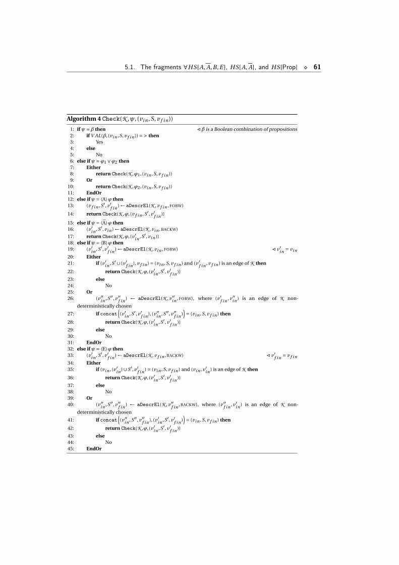
5.1. The fragments ∀HS[A, A,B ,E ], HS[A, A], and HS[Prop] ¦ 61
Algorithm 4 Check(K ,ψ, (vi n ,S, v f i n))
1: if ψ=β then / β is a Boolean combination of propositions2: if V AL(β, (vi n ,S, v f i n )) => then3: Yes4: else5: No6: else if ψ=ϕ1 ∨ϕ2 then7: Either8: return Check(K ,ϕ1, (vi n ,S, v f i n ))9: Or
10: return Check(K ,ϕ2, (vi n ,S, v f i n ))11: EndOr12: else if ψ= ⟨A⟩ϕ then13: (v f i n ,S′, v ′
f i n ) ← aDescrEl(K , v f i n , FORW)
14: return Check(K ,ϕ, (v f i n ,S′, v ′f i n ))
15: else if ψ= ⟨A⟩ϕ then16: (v ′
i n ,S′, vi n ) ← aDescrEl(K , vi n , BACKW)
17: return Check(K ,ϕ, (v ′i n ,S′, vi n ))
18: else if ψ= ⟨B⟩ϕ then19: (v ′
i n ,S′, v ′f i n ) ← aDescrEl(K , vi n , FORW) / v ′
i n = vi n
20: Either21: if (v ′
i n ,S′∪ v ′f i n , v f i n ) = (vi n ,S, v f i n ) and (v ′
f i n , v f i n ) is an edge of K then
22: return Check(K ,ϕ, (v ′i n ,S′, v ′
f i n ))
23: else24: No25: Or26: (v ′′
i n ,S′′, v ′′f i n ) ← aDescrEl(K , v ′′
i n , FORW), where (v ′f i n , v ′′
i n ) is an edge of K non-
deterministically chosen
27: if concat((v ′
i n ,S′, v ′f i n ), (v ′′
i n ,S′′, v ′′f i n )
)= (vi n ,S, v f i n ) then
28: return Check(K ,ϕ, (v ′i n ,S′, v ′
f i n ))
29: else30: No31: EndOr32: else if ψ= ⟨E⟩ϕ then33: (v ′
i n ,S′, v ′f i n ) ← aDescrEl(K , v f i n , BACKW) / v ′
f i n = v f i n
34: Either35: if (vi n , v ′
i n ∪S′, v ′f i n ) = (vi n ,S, v f i n ) and (vi n , v ′
i n ) is an edge of K then
36: return Check(K ,ϕ, (v ′i n ,S′, v ′
f i n ))
37: else38: No39: Or40: (v ′′
i n ,S′′, v ′′f i n ) ← aDescrEl(K , v ′′
f i n , BACKW), where (v ′′f i n , v ′
i n ) is an edge of K non-
deterministically chosen
41: if concat((v ′′
i n ,S′′, v ′′f i n ), (v ′
i n ,S′, v ′f i n )
)= (vi n ,S, v f i n ) then
42: return Check(K ,ϕ, (v ′i n ,S′, v ′
f i n ))
43: else44: No45: EndOr
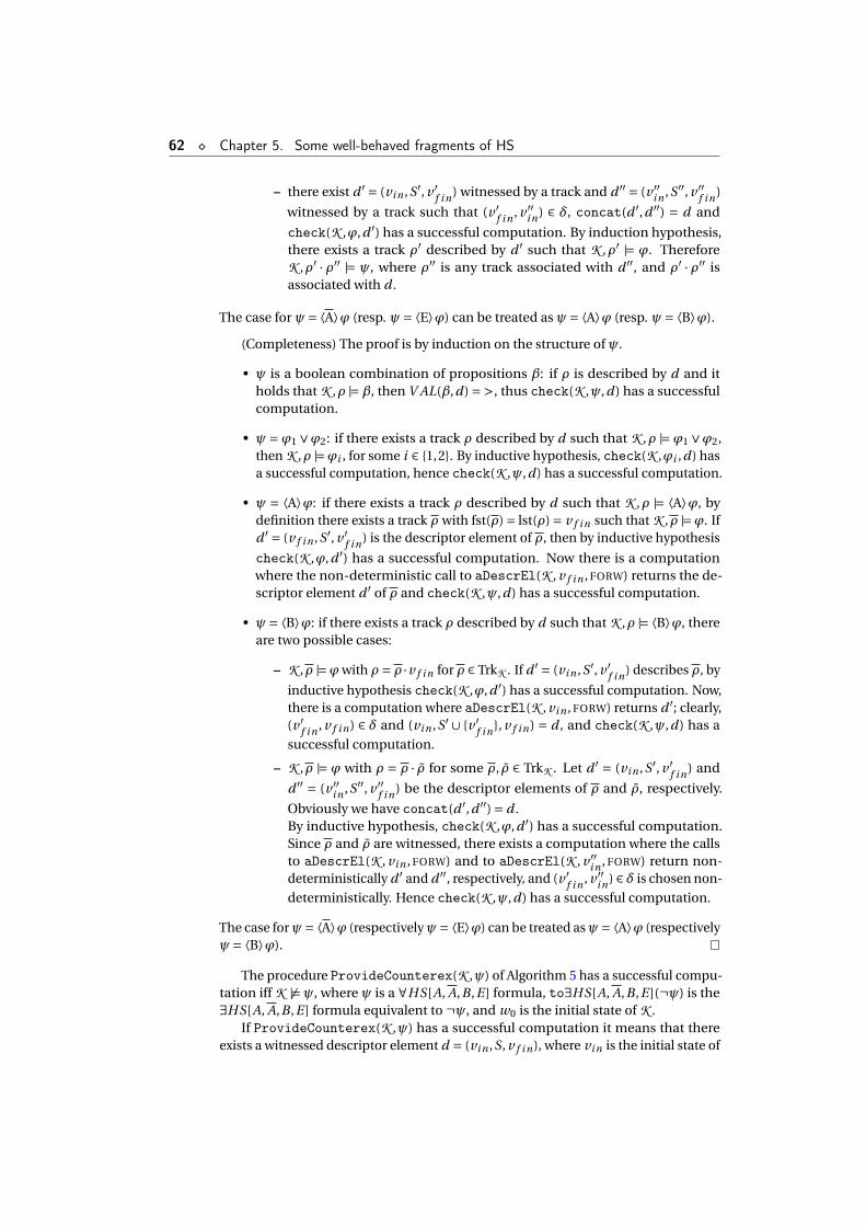
62 ¦ Chapter 5. Some well-behaved fragments of HS
– there exist d ′ = (vi n ,S′, v ′f i n) witnessed by a track and d ′′ = (v ′′
i n ,S′′, v ′′f i n)
witnessed by a track such that (v ′f i n , v ′′
i n) ∈ δ, concat(d ′,d ′′) = d and
check(K ,ϕ,d ′) has a successful computation. By induction hypothesis,there exists a track ρ′ described by d ′ such that K ,ρ′ |= ϕ. ThereforeK ,ρ′ ·ρ′′ |= ψ, where ρ′′ is any track associated with d ′′, and ρ′ ·ρ′′ isassociated with d .
The case for ψ= ⟨A⟩ϕ (resp. ψ= ⟨E⟩ϕ) can be treated as ψ= ⟨A⟩ϕ (resp. ψ= ⟨B⟩ϕ).
(Completeness) The proof is by induction on the structure of ψ.
• ψ is a boolean combination of propositions β: if ρ is described by d and itholds that K ,ρ |=β, then V AL(β,d) =>, thus check(K ,ψ,d) has a successfulcomputation.
• ψ=ϕ1 ∨ϕ2: if there exists a track ρ described by d such that K ,ρ |=ϕ1 ∨ϕ2,then K ,ρ |=ϕi , for some i ∈ 1,2. By inductive hypothesis, check(K ,ϕi ,d) hasa successful computation, hence check(K ,ψ,d) has a successful computation.
• ψ = ⟨A⟩ϕ: if there exists a track ρ described by d such that K ,ρ |= ⟨A⟩ϕ, bydefinition there exists a track ρ with fst(ρ) = lst(ρ) = v f i n such that K ,ρ |=ϕ. Ifd ′ = (v f i n ,S′, v ′
f i n) is the descriptor element of ρ, then by inductive hypothesis
check(K ,ϕ,d ′) has a successful computation. Now there is a computationwhere the non-deterministic call to aDescrEl(K , v f i n , FORW) returns the de-scriptor element d ′ of ρ and check(K ,ψ,d) has a successful computation.
• ψ= ⟨B⟩ϕ: if there exists a track ρ described by d such that K ,ρ |= ⟨B⟩ϕ, thereare two possible cases:
– K ,ρ |=ϕwith ρ = ρ ·v f i n for ρ ∈ TrkK . If d ′ = (vi n ,S′, v ′f i n) describes ρ, by
inductive hypothesis check(K ,ϕ,d ′) has a successful computation. Now,there is a computation where aDescrEl(K , vi n , FORW) returns d ′; clearly,(v ′
f i n , v f i n) ∈ δ and (vi n ,S′∪ v ′f i n, v f i n) = d , and check(K ,ψ,d) has a
successful computation.
– K ,ρ |= ϕ with ρ = ρ · ρ for some ρ, ρ ∈ TrkK . Let d ′ = (vi n ,S′, v ′f i n) and
d ′′ = (v ′′i n ,S′′, v ′′
f i n) be the descriptor elements of ρ and ρ, respectively.
Obviously we have concat(d ′,d ′′) = d .By inductive hypothesis, check(K ,ϕ,d ′) has a successful computation.Since ρ and ρ are witnessed, there exists a computation where the callsto aDescrEl(K , vi n , FORW) and to aDescrEl(K , v ′′
i n , FORW) return non-deterministically d ′ and d ′′, respectively, and (v ′
f i n , v ′′i n) ∈ δ is chosen non-
deterministically. Hence check(K ,ψ,d) has a successful computation.
The case forψ= ⟨A⟩ϕ (respectivelyψ= ⟨E⟩ϕ) can be treated asψ= ⟨A⟩ϕ (respectivelyψ= ⟨B⟩ϕ).
The procedure ProvideCounterex(K ,ψ) of Algorithm 5 has a successful compu-tation iff K 6|=ψ, where ψ is a ∀HS[A, A,B ,E ] formula, to∃HS[A, A,B ,E ](¬ψ) is the∃HS[A, A,B ,E ] formula equivalent to ¬ψ, and w0 is the initial state of K .
If ProvideCounterex(K ,ψ) has a successful computation it means that thereexists a witnessed descriptor element d = (vi n ,S, v f i n), where vi n is the initial state of
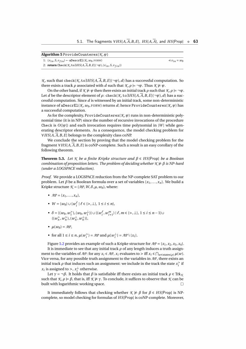
5.1. The fragments ∀HS[A, A,B ,E ], HS[A, A], and HS[Prop] ¦ 63
Algorithm 5 ProvideCounterex(K ,ψ)
1: (vi n ,S, v f i n ) ← aDescrEl(K , w0, FORW) / vi n = w0
2: return Check(K ,to∃HS[A, A,B ,E ](¬ψ), (vi n ,S, v f i n ))
K , such that check(K ,to∃HS[A, A,B ,E ](¬ψ),d) has a successful computation. Sothere exists a track ρ associated with d such that K ,ρ |= ¬ψ. Thus K 6|=ψ.
On the other hand, if K 6|=ψ then there exists an initial track ρ such that K ,ρ |= ¬ψ.Let d be the descriptor element of ρ: check(K ,to∃HS[A, A,B ,E ](¬ψ),d) has a suc-cessful computation. Since d is witnessed by an initial track, some non-deterministicinstance of aDescrEl(K , w0, FORW) returns d ; hence ProvideCounterex(K ,ψ) hasa successful computation.
As for the complexity, ProvideCounterex(K ,ψ) runs in non-deterministic poly-nomial time (it is in NP) since the number of recursive invocations of the procedureCheck is O(|ψ|) and each invocation requires time polynomial in |W | while gen-erating descriptor elements. As a consequence, the model checking problem for∀HS[A, A,B ,E ] belongs to the complexity class coNP.
We conclude the section by proving that the model checking problem for thefragment ∀HS[A, A,B ,E ] is coNP-complete. Such a result is an easy corollary of thefollowing theorem.
Theorem 5.3. Let K be a finite Kripke structure and β ∈ HS[Prop] be a Booleancombination of proposition letters. The problem of deciding whether K 6|=β is NP-hard(under a LOGSPACE reduction).
Proof. We provide a LOGSPACE reduction from the NP-complete SAT problem to ourproblem. Let β be a Boolean formula over a set of variables x1, . . . , xn. We build aKripke structure K = (AP ,W,δ,µ, w0), where:
• AP = x1, . . . , xn,
• W = w0∪ w`i | ` ∈ >,⊥, 1 ≤ i ≤ n,
• δ= (w0, w>1 ), (w0, w⊥
1 )∪ (w`i , wm
i+1) | `,m ∈ >,⊥, 1 ≤ i ≤ n −1∪(w>
n , w>n ), (w⊥
n , w⊥n ),
• µ(w0) = AP ,
• for all 1 ≤ i ≤ n, µ(w>i ) = AP and µ(w⊥
i ) = AP \ xi .
Figure 5.2 provides an example of such a Kripke structure for AP = x1, x2, x3, x4.It is immediate to see that any initial track ρ of any length induces a truth assign-
ment to the variables of AP : for any xi ∈ AP , xi evaluates to > iff xi ∈⋂w∈states(ρ)µ(w).
Vice versa, for any possible truth assignment to the variables in AP , there exists aninitial track ρ that induces such an assignment: we include in the track the state x>
i ifxi is assigned to >, x⊥
i otherwise.Let γ = ¬β. It holds that β is satisfiable iff there exists an initial track ρ ∈ TrkK
such that K ,ρ |=β, that is, iff K 6|= γ. To conclude, it suffices to observe that K can bebuilt with logarithmic working space.
It immediately follows that checking whether K 6|= β for β ∈ HS[Prop] is NP-complete, so model checking for formulas of HS[Prop] is coNP-complete. Moreover,
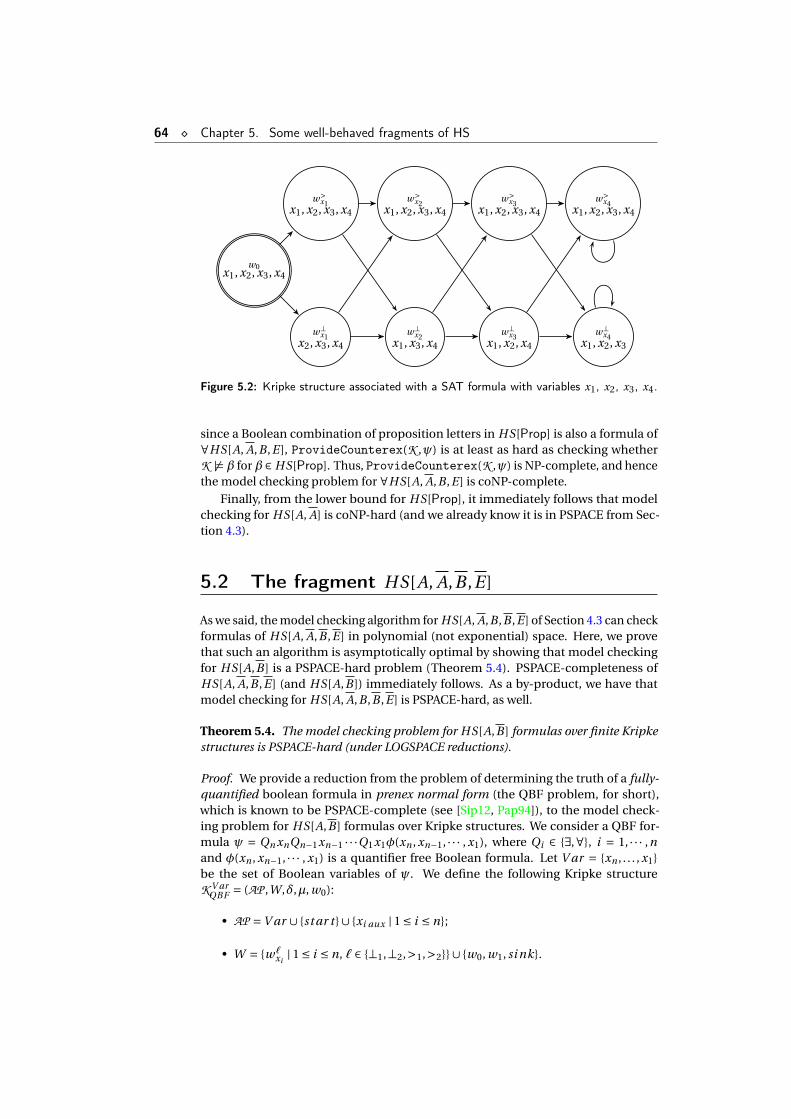
64 ¦ Chapter 5. Some well-behaved fragments of HS
w0x1, x2, x3, x4
w>x1
x1, x2, x3, x4
w⊥x1
x2, x3, x4
w>x2
x1, x2, x3, x4
w⊥x2
x1, x3, x4
w>x3
x1, x2, x3, x4
w⊥x3
x1, x2, x4
w>x4
x1, x2, x3, x4
w⊥x4
x1, x2, x3
Figure 5.2: Kripke structure associated with a SAT formula with variables x1, x2, x3, x4.
since a Boolean combination of proposition letters in HS[Prop] is also a formula of∀HS[A, A,B ,E ], ProvideCounterex(K ,ψ) is at least as hard as checking whetherK 6|=β for β ∈ HS[Prop]. Thus, ProvideCounterex(K ,ψ) is NP-complete, and hencethe model checking problem for ∀HS[A, A,B ,E ] is coNP-complete.
Finally, from the lower bound for HS[Prop], it immediately follows that modelchecking for HS[A, A] is coNP-hard (and we already know it is in PSPACE from Sec-tion 4.3).
5.2 The fragment HS[A, A,B ,E ]
As we said, the model checking algorithm for HS[A, A,B ,B ,E ] of Section 4.3 can checkformulas of HS[A, A,B ,E ] in polynomial (not exponential) space. Here, we provethat such an algorithm is asymptotically optimal by showing that model checkingfor HS[A,B ] is a PSPACE-hard problem (Theorem 5.4). PSPACE-completeness ofHS[A, A,B ,E ] (and HS[A,B ]) immediately follows. As a by-product, we have thatmodel checking for HS[A, A,B ,B ,E ] is PSPACE-hard, as well.
Theorem 5.4. The model checking problem for HS[A,B ] formulas over finite Kripkestructures is PSPACE-hard (under LOGSPACE reductions).
Proof. We provide a reduction from the problem of determining the truth of a fully-quantified boolean formula in prenex normal form (the QBF problem, for short),which is known to be PSPACE-complete (see [Sip12, Pap94]), to the model check-ing problem for HS[A,B ] formulas over Kripke structures. We consider a QBF for-mula ψ = Qn xnQn−1xn−1 · · ·Q1x1φ(xn , xn−1, · · · , x1), where Qi ∈ ∃,∀, i = 1, · · · ,nand φ(xn , xn−1, · · · , x1) is a quantifier free Boolean formula. Let V ar = xn , . . . , x1be the set of Boolean variables of ψ. We define the following Kripke structureK V ar
QBF = (AP ,W,δ,µ, w0):
• AP =V ar ∪ st ar t ∪ xi aux | 1 ≤ i ≤ n;
• W = w`xi| 1 ≤ i ≤ n, ` ∈ ⊥1,⊥2,>1,>2∪ w0, w1, si nk.
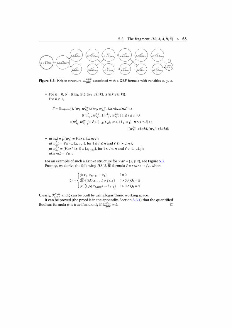
5.2. The fragment HS[A, A,B ,E ] ¦ 65
w0x, y, z, st ar t
w1x, y, z, st ar t
w>1x
x, y, z, xaux
w⊥1x
y, z, xaux
w>2x
x, y, z, xaux
w⊥2x
y, z, xaux
w>1y
x, y, z, yaux
w⊥1y
x, z, yaux
w>2y
x, y, z, yaux
w⊥2y
x, z, yaux
w>1z
x, y, z, zaux
w⊥1z
x, y, zaux
w>2z
x, y, z, zaux
w⊥2z
x, y, zaux
si nkx, y, z
Figure 5.3: Kripke structure K x,y,zQBF associated with a QBF formula with variables x, y, z.
• For n = 0, δ= (w0, w1), (w1, si nk), (si nk, si nk).For n ≥ 1,
δ= (w0, w1), (w1, w>1xn
), (w1, w⊥1xn
), (si nk, si nk) ∪(w>1
xi, w>2
xi), (w⊥1
xi, w⊥2
xi) | 1 ≤ i ≤ n ∪
(w`xi
, wmxi−1
) | ` ∈ ⊥2,>2, m ∈ ⊥1,>1, n ≤ i ≤ 2 ∪(w>2
x1, si nk), (w⊥2
x1, si nk);
• µ(w0) =µ(w1) =V ar ∪ st ar t ;µ(w`
xi) =V ar ∪ xi aux , for 1 ≤ i ≤ n and ` ∈ >1,>2;
µ(w`xi
) = (V ar \ xi )∪ xi aux , for 1 ≤ i ≤ n and ` ∈ ⊥1,⊥2;µ(si nk) =V ar .
For an example of such a Kripke structure for V ar = x, y, z, see Figure 5.3.From ψ, we derive the following HS[A,B ] formula ξ= st ar t → ξn , where
ξi =
φ(xn , xn−1, · · ·x1) i = 0
⟨B⟩((⟨A⟩xi aux )∧ξi−1)
i > 0∧Qi =∃[B ]
((⟨A⟩xi aux ) → ξi−1
)i > 0∧Qi =∀
.
Clearly, K V arQBF and ξ can be built by using logarithmic working space.
It can be proved (the proof is in the appendix, Section A.3.1) that the quantifiedBoolean formula ψ is true if and only if K V ar
QBF |= ξ.

6Conclusions
In this final chapter we summarize the results achieved so far (see Figure 6.1 for avisual report).
In Chapter 3 we have proved that the (full) HS model checking problem is decid-able with a non-elementary upper bound, by following [MMPP14]. The cornerstoneof the decidability proof is the notion of BEk -descriptor, which allows us to obtain afinite representation of a possibly infinite set of equivalent tracks. Since the numberof BEk -descriptors is always finite, the decidability of the model checking problemfor HS over finite Kripke structures easily follows. In addition, we have provided a no-tion, correspondence between descriptors, which precisely captures k-equivalencebetween tracks. Finally, we have proved that the HS model checking problem isEXPSPACE-hard, provided that a succinct encoding of formulas is used (otherwisewe can only prove that it is PSPACE-hard).
In Chapter 4 we have showed that formulas of the fragment HS[A, A,B ,B ,E ] (andof the symmetric HS[A, A,E ,B ,E ]) can be checked with exponential working space.The proposed algorithm rests on a contraction method that allows us to restrict theverification of the input formula to a finite subset of tracks of bounded size, calledtrack representatives. These are determined by evaluating k-indistinguishabilityamong descriptor elements, a notion which allows both to determine if two tracksare associated with the same Bk -descriptor (without building it explicitly), and tocalculate an upper bound to the length of representatives. In the end, we have provedthat the model checking problem for HS[A, A,B ,B ,E ] is NEXP-hard, provided that asuccinct encoding of formulas is used.
In Chapter 5 we have clarified the complexity picture of some HS fragments,∀HS[A, A,B ,E ], HS[A, A] and HS[A, A,B ,E ], whose formulas are expressive enoughto capture typical interval properties of transition systems, while keeping the modelchecking complexity lower, comparable to that of point-based temporal logics.
Clearly, our analysis of HS model checking is innovative, thus many problemsare still open. For example, the exact complexity of the full logic is unknown: itranges from PSPACE to non-ELEMENTARY (in the non-succinct case), quite a big gap!Even some apparently easy fragments are still unsolved (e.g., HS[A, A] is in betweencoNP and PSPACE). It is evident that if B and E modalities are not involved, modelchecking for such fragments is in PSPACE. As soon as one of these two is added, theexpressiveness of fragments increases (e.g., metric properties about the length of
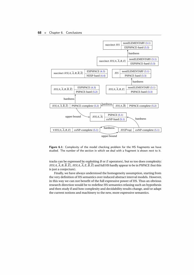
68 ¦ Chapter 6. Conclusions
HS[A, A,B ,E ] PSPACE-complete (5.2) HS[A,B ] PSPACE-complete (5.2)
HS[A, A]PSPACE (5.1)
coNP-hard (5.1)
∀HS[A, A,B ,E ] coNP-complete (5.1) HS[Prop] coNP-complete (5.1)
HS[A, A,B ,B ,E ]EXPSPACE (4.3)
PSPACE-hard (5.2)
succinct HS[A, A,B ,B ,E ]EXPSPACE (4.3)
NEXP-hard (4.4)
HS[A, A,B ,E ]nonELEMENTARY (3.1)
PSPACE-hard (3.3)
HSnonELEMENTARY (3.1)
PSPACE-hard (3.3)
succinct HS[A, A,B ,E ]nonELEMENTARY (3.1)
EXPSPACE-hard (3.3)
succinct HSnonELEMENTARY (3.1)
EXPSPACE-hard (3.3)
hardness
upper bound
hardness
hardness
hardness
upper bound
hardness
hardness
Figure 6.1: Complexity of the model checking problem for the HS fragments we havestudied. The number of the section in which we deal with a fragment is shown next to it.
tracks can be expressed by exploiting B or E operators), but so too does complexity:HS[A, A,B ,B ,E ], HS[A, A,E ,B ,E ] and full HS hardly appear to be in PSPACE (but thisis just a conjecture).
Finally, we have always understood the homogeneity assumption, starting fromthe very definition of HS semantics over induced abstract interval models. However,in this way we can not benefit of the full expressive power of HS. Thus an obviousresearch direction would be to redefine HS semantics relaxing such an hypothesisand then study if and how complexity and decidability results change, and/or adaptthe current notions and machinery to the new, more expressive semantics.
AAppendix
ContentsA.1 Proofs of Chapter 3 . . . . . . . . . . . . . . . . . . . . . . . . . . . . 69
A.1.1 Proof of Lemma 3.9 . . . . . . . . . . . . . . . . . . . . . . . . . 69A.1.2 Proof of Lemma 3.10 . . . . . . . . . . . . . . . . . . . . . . . . 70
A.2 Proofs of Chapter 4 . . . . . . . . . . . . . . . . . . . . . . . . . . . . 71A.2.1 Proof of Lemma 4.1 . . . . . . . . . . . . . . . . . . . . . . . . . 71A.2.2 Proof of Theorem 4.20 . . . . . . . . . . . . . . . . . . . . . . . 72A.2.3 Proof of Theorem 4.24 . . . . . . . . . . . . . . . . . . . . . . . 74A.2.4 Proof of Lemma 4.25 . . . . . . . . . . . . . . . . . . . . . . . . 74
A.3 Proofs of Chapter 5 . . . . . . . . . . . . . . . . . . . . . . . . . . . . 75A.3.1 Proof of Theorem 5.4 . . . . . . . . . . . . . . . . . . . . . . . . 75
A.1 Proofs of Chapter 3
A.1.1 Proof of Lemma 3.9
Proof. The proof is by induction on n ≥ 0. Let DBEk and D ′BEk
be the BEk -descriptors
for ρ and ρ′, respectively.Base case (n = 0). Since K ,ρ |= p ⇐⇒ K ,ρ′ |= p, for any p ∈ AP , the roots of DBEk
and D ′BEk
are labelled by the same set of proposition letters and the descriptors arecorresponding up to depth 0.
Inductive step (n ≥ 1). We preliminarily show that if ρ and ρ′ are k-equivalentwith respect to all formulas ϕ with Nest(ϕ) ≤ n, then for any track ρ ∈ TrkK , withfst(ρ) = lst(ρ), there is a track ρ′ ∈ TrkK , with fst(ρ′) = lst(ρ′), such that, for all HSformulas ψ, with Nest(ψ) ≤ n −1 and NestBE(ψ) ≤ k, K ,ρ |=ψ ⇐⇒ K ,ρ′ |=ψ. Theproof is by contradiction. Suppose that there is a track ρ ∈ TrkK , with fst(ρ) = lst(ρ),such that, for all tracks ρ′ ∈ TrkK , with fst(ρ′) = lst(ρ′), there exists a formula ψ, withNest(ψ) ≤ n−1 and NestBE(ψ) ≤ k, such that K ,ρ |=ψ and K ,ρ′ 6|=ψ. Let H be the setof those tracks ρ such that fst(ρ) = lst(ρ′). H can be partitioned into a finite number
70 ¦ Appendix A. Appendix
of classes, say s ≥ 1, each one containing k-descriptor equivalent tracks of H (recallthat k-descriptor equivalence is an equivalence relation of finite index). Now, letρ′
1,ρ′2, . . . ,ρ′
s be a set of track representatives, chosen one for each equivalence classinduced by ∼k on H (for all 1 ≤ i < j ≤ s, ρ′
i and ρ′j have distinct BEk -descriptors).
By Theorem 3.2, tracks which are k-descriptor equivalent satisfy the same set offormulas ψ′, with NestBE(ψ′) ≤ k. So there are formulas ψ1, . . . ,ψs such that, for all1 ≤ i ≤ s, Nest(ψi ) ≤ n−1, NestBE(ψi ) ≤ k, K ,ρ |=ψi , and K ,ρ′
i 6|=ψi . It easily followsthat K ,ρ |= ψ1 ∧ψ2 ∧ ·· · ∧ψs and, for all 1 ≤ i ≤ s, K ,ρ′
i |= ¬ψ1 ∨¬ψ2 ∨ ·· · ∨¬ψs .Hence, K ,ρ |= ⟨A⟩(ψ1 ∧ψ2 ∧·· ·∧ψs ) and K ,ρ′ |= [A](¬ψ1 ∨¬ψ2 ∨·· ·∨¬ψs ), that is,K ,ρ′ 6|= ⟨A⟩(ψ1 ∧ψ2 ∧·· ·∧ψs ), which is a contradiction.
Thus, we have proved that for any track ρ ∈ TrkK , with fst(ρ) = lst(ρ), there ex-ists a track ρ′ ∈ TrkK , with fst(ρ′) = lst(ρ′), such that, for all HS formulas ψ, withNest(ψ) ≤ n−1 and NestBE(ψ) ≤ k, K ,ρ |=ψ ⇐⇒ K ,ρ′ |=ψ. By the inductive hypoth-esis, ρ and ρ′ are associated with corresponding BEk -descriptors up to depth n −1.Symmetrically, we can show that for any track ρ′ ∈ TrkK , with fst(ρ′) = lst(ρ′), thereexists ρ ∈ TrkK , with fst(ρ) = lst(ρ), such that ρ′ and ρ are associated with correspond-ing BEk -descriptors up to depth n −1. In this way, we have proved the conditionfor modality A of Definition 3.8. The conditions for modalities A, B , and E can beproved in a very similar way. In particular, as a consequence of the fact that ρ andρ′ are k-equivalent with respect to all HS formulas ψ, with Nest(ψ) ≤ n and n ≥ 1, itholds that K ,ρ |= ⟨A⟩> ⇐⇒ K ,ρ′ |= ⟨A⟩>. It follows that DBEk has an A-successor ifand only if D ′
BEkhas one. The same holds for E-successors.
Let us now consider the condition for modality B of Definition 3.8.First of all, we show that for any track ρ ∈ Pref(ρ), there exists a track ρ′ ∈ Pref(ρ′)
such that for all formulas ψ of HS, having Nest(ψ) ≤ n − 1 and NestBE(ψ) ≤ k − 1,K ,ρ |=ψ ⇐⇒ K ,ρ′ |=ψ. The proof is again by contradiction. Suppose that thereexists a track ρ ∈ Pref(ρ) such that, for all tracks ρ′ ∈ Pref(ρ′), there exists a formula ψ,with Nest(ψ) ≤ n −1 and NestBE(ψ) ≤ k −1, such that K ,ρ |=ψ and K ,ρ′ 6|=ψ. Now,let us consider the tracks ρ′
1,ρ′2, · · · ,ρ′
s (for some s ∈N) which are prefixes of ρ′ andare associated with distinct subtrees of depth k −1 of the BEk -descriptor for ρ′ (thenumber of these tracks is obviously finite). So there are formulas ψ1, . . . ,ψs suchthat, for all 1 ≤ i ≤ s, Nest(ψi ) ≤ n −1, NestBE(ψi ) ≤ k −1, K ,ρ |=ψi , and K ,ρ′
i 6|=ψi .Thus, K ,ρ |= ψ1 ∧ψ2 ∧ ·· ·∧ψs and for all i , K ,ρ′
i |= ¬ψ1 ∨¬ψ2 ∨ ·· ·∨¬ψs . Hencewe have K ,ρ |= ⟨B⟩(ψ1 ∧ψ2 ∧·· ·∧ψs ) and K ,ρ′ |= [B ](¬ψ1 ∨¬ψ2 ∨·· ·∨¬ψs ), that isK ,ρ′ 6|= ⟨B⟩(ψ1 ∧ψ2 ∧·· ·∧ψs ), which leads to a contradiction.
We have proved that for any track ρ ∈ Pref(ρ), there exists a track ρ′ ∈ Pref(ρ′)such that, for all formulas ψ of HS, having Nest(ψ) ≤ n −1 and NestBE(ψ) ≤ k −1,K ,ρ |=ψ ⇐⇒ K ,ρ′ |=ψ. By the inductive hypothesis, ρ and ρ′ are associated withcorresponding BEk−1-descriptors up to depth n −1. Symmetrically, we can showthat for any track ρ′ ∈ Pref(ρ′), there exists a track ρ ∈ Pref(ρ) such that ρ′ and ρ areassociated with corresponding BEk−1-descriptors up to depth n −1.
In this way, we have proved the condition for modality B of Definition 3.8. Thecondition for modality E can be proved in a symmetrical way.
A.1.2 Proof of Lemma 3.10
Proof. The proof is by induction on n ≥ 0.Base case (n = 0). Consider the descriptors DBEk , D ′
BEk, DBEk |k−1, and D ′
BEk|k−1.
Since the roots of DBEk and D ′BEk
are labelled by the same set of proposition letters,
A.2. Proofs of Chapter 4 ¦ 71
the roots of DBEk |k−1 and D ′BEk
|k−1 are labelled by the same set of proposition lettersas well.
Inductive step (n > 0). Let ρ,ρ′ ∈ TrkK be two witnesses for DBEk and for D ′BEk
,
respectively (and thus for DBEk |k−1 and D ′BEk
|k−1, respectively). Consider a track
ρ ∈ TrkK , with fst(ρ) = lst(ρ). The BEk -descriptor ˜DBEk for ρ is an A-successor ofDBEk , and ˜DBEk |k−1 is an A-successor of DBEk |k−1. Since DBEk and D ′
BEkare corre-
sponding up to depth n, there exists a track ρ ∈ TrkK , with fst(ρ) = lst(ρ′), describedby DBEk , such that ˜DBEk and DBEk are corresponding up to depth n −1. By the in-ductive hypothesis, ˜DBEk |k−1 and DBEk |k−1 are corresponding up to depth n−1 (and,obviously, DBEk |k−1 is an A-successor of D ′
BEk|k−1).
Let us consider now a track ρ, with (lst(ρ), fst(ρ)) ∈ δ and ρ · ρ ∈ TrkK . The BEk -descriptor ˆDBEk of ρ · ρ is a B-successor of DBEk and ˆDBEk |k−1 is a B-successor ofDBEk |k−1. Since DBEk and D ′
BEkare corresponding up to depth n, there exists a track
ρ such that (lst(ρ′), fst(ρ)) ∈ δ, ρ′ · ρ is described by ˇDBEk , and ˆDBEk and ˇDBEk arecorresponding up to depth n−1. By the inductive hypothesis, ˆDBEk |k−1 and ˇDBEk |k−1
are corresponding up to depth n −1 (and, obviously, ˇDBEk |k−1 is a B-successor ofD ′
BEk|k−1).
Finally (only for cases with k ≥ 2), let us consider a subtree of depth k−2 linked tothe root of DBEk |k−1 via a B-edge. In this case, there exists (at least) a subtree of DBEk ,say Sk−1, such that Sk−1|k−2 is the considered subtree of DBEk |k−1. Since DBEk andD ′
BEkare corresponding up to depth n, there exists a subtree S ′
k−1 of D ′BEk
, connected
to the root of D ′BEk
via a B-edge, corresponding to Sk−1 up to depth n −1. By the
inductive hypothesis Sk−1|k−2 and S ′k−1|k−2 are corresponding up to depth n −1 (the
latter is a subtree of D ′BEk
|k−1 connected to the root of D ′BEk
|k−1 via a B-edge).The remaining cases can be dealt with analogously.
A.2 Proofs of Chapter 4
A.2.1 Proof of Lemma 4.1
In the proof, we will exploit the fact that if two tracks in TrkK have the same Bk+1-descriptor, then they also have the same Bk -descriptor. The latter can indeed beobtained from the former by removing the nodes at depth k +1 (leaves) and thendeleting isomorphic subtrees possibly originated by the removal.
Proof. By induction on k ∈N.k = 0: if ρ1 and ρ2 are associated with the descriptor element (vi n ,S, v f i n), and
ρ′1 and ρ′
2 with (v ′i n ,S′, v ′
f i n), then ρ1 ·ρ′1 and ρ2 ·ρ′
2 are both represented by the
descriptor element (vi n ,S ∪ v f i n , v ′i n∪S′, v ′
f i n).
k > 0: let DBk be the Bk -descriptor of ρ1 ·ρ′1 and D ′
Bkthe Bk -descriptor of ρ2 ·ρ′
2:
their roots are the same (as for k = 0); let us now consider a generic prefix ρ of ρ1 ·ρ′1:
• if ρ is a proper prefix of ρ1, since ρ1 and ρ2 have the same Bk -descriptor, thereexists a prefix ρ of ρ2 associated with the same subtree as ρ of depth k −1 inthe descriptor of ρ1 (and ρ2);
• for ρ = ρ1, it holds that ρ1 and ρ2 have the same Bk−1-descriptor because theyhave the same Bk -descriptor;
72 ¦ Appendix A. Appendix
• if ρ is a proper prefix of ρ1 ·ρ′1 such that ρ = ρ1 ·ρ1 for some prefix ρ1 of ρ′
1, thentwo cases have to be taken into account:
– if |ρ1| = 1, then ρ1 = v ′i n ; but also fst(ρ′
2) = v ′i n . Let us now consider the
Bk−1-descriptors for ρ1 · v ′i n and ρ2 · v ′
i n : the labels of the roots are thesame, (vi n ,S ∪ v f i n, v ′
i n), then the subtrees of depth k −2 are exactly thesame as those of ρ1 and ρ2’s Bk−1-descriptor, (possibly) with the additionof the Bk−2-descriptor of ρ1 (which is equal to that of ρ2). Thus ρ1 · v ′
i nand ρ2 · v ′
i n have the same Bk−1-descriptor;
– otherwise, since ρ1 is a prefix of ρ′1 of length at least 2, and ρ′
1 and ρ′2 have
the same Bk -descriptor, there exists a prefix ρ2 of ρ′2 associated with the
same subtree of depth k −1 as ρ1 (in the Bk -descriptor of ρ′1). Hence, by
inductive hypothesis, ρ1 · ρ1 and ρ2 · ρ2 have the same Bk−1-descriptor.
Therefore we have shown that for any proper prefix of ρ1 ·ρ′1 there exists a proper
prefix of ρ2 · ρ′2 having the same Bk−1-descriptor. The inverse can be shown by
symmetry. Thus DBk is equal to D ′Bk
.
A.2.2 Proof of Theorem 4.20
Proof. The proof is by induction on i ≥ u +1.(Case i = u +1) We consider two cases:
1. if ρd s (u) = ρd s (u +1) = d ∈ C , then we have Q−2(u) = C \ d, Q−1(u) = d, ;=Q0(u) =Q1(u) = ·· · =Qs (u). Moreover, it holds Q−2(u +1) = C \ d, Q−1(u) =;,Q0(u) = d and ; = Q1(u) = Q2(u) = ·· · = Qs (u). c(u) >lex c(u + 1) and thethesis follows.
2. if d ,d ′ ∈ C , d 6= d ′ and ρd s (u) = d , ρd s (u+1) = d ′, then we have Q−2(u) = C \d,Q−1(u) = d, ;=Q0(u) =Q1(u) = ·· · =Qs (u). Moreover, Q−2(u+1) = C \d ,d ′,Q−1(u) = d ,d ′, ; = Q0(u) = Q1(u) = ·· · = Qs (u), c(u) >l ex c(u +1), implyingthe thesis.
(Case i > u+1) In the following we say that ρd s (`) and ρd s (m) (`< m) are consecutiveoccurrences of a descriptor element d if there are no other occurrences of d inρd s (`+1,m −1). We consider the following cases:
1. If ρd s (i ) is the first occurrence of d ∈ C , then d ∈ Q−2(i −1), d ∈ Q−1(i ) andc(i −1) >lex c(i ).
2. If ρd s (i ) is the second occurrence of d ∈ C , according to the definition, ρd s (i )can not be 1-indistinguishable from the previous occurrence of d . Therefored ∈ Q−1(i −1) (ρd s (u, i −1) contains the first occurrence of d) and d ∈ Q0(i ),proving that c(i −1) >l ex c(i ).
3. If ρd s (i ) is at least the third occurrence of d but ρd s (i ) is not 1-indistinguishablefrom the immediately preceding occurrence of d ρd s (i ′), (with i ′ < i ), thenDElm(ρd s (u, i ′−1)) ⊂ DElm(ρd s (u, i −1)). Hence, there exists a first occur-rence of some d ′ ∈ C in ρd s (i ′+1, i −1), say ρd s ( j ) = d ′, for i ′+1 ≤ j ≤ i −1.Thus d ∈Q−1( j ), · · · , d ∈Q−1(i −1) and d ∈Q0(i ), proving that c(i −1) >lex c(i ).
A.2. Proofs of Chapter 4 ¦ 73
4. In the remaining cases we assume that ρd s (i ) is at least the third occurrenceof d ∈ C . If ρd s (i −1) and ρd s (i ) are both occurrences of d ∈ C and ρd s (i −1)is t-indistinguishable, for some t > 0, and not (t +1)-indistinguishable, fromthe immediately preceding occurrence of d , then ρd s (i − 1) and ρd s (i ) areexactly (t + 1)-indistinguishable. So d ∈ Qt (i − 1) and d ∈ Qt+1(i ), implyingthat c(i −1) >lex c(i ) (as a particular case, if ρd s (i −1) and the immediatelypreceding occurrence are not 1-indistinguishable, then ρd s (i −1) and ρd s (i )are at most 1-indistinguishable).
5. If ρd s (i ) is exactly 1-indistinguishable from the immediately preceding occur-rence of d , ρd s ( j ), j < i −1, then DElm(ρd s (u, j −1)) = DElm(ρd s (u, i −1)),and there are no first occurrences of any d ′ ∈ C in ρd s ( j , i −1). If ρd s ( j ) is not1-indistinguishable from its previous occurrence of d , it immediately followsthat d ∈Q0( j ), · · · , d ∈Q0(i −1) and d ∈Q1(i ), implying that c(i −1) >l ex c(i ).
Otherwise, there exists j < i ′ < i s.t. ρd s (i ′) = d ′′ ∈ C is not 1-indistinguishablefrom any occurrence of d ′′ before j (as a matter of fact, if this was not the case,ρd s (i ) and ρd s ( j ) would be 2-indistinguishable); in particular, ρd s (i ′) is not 1-indistinguishable from the last occurrence of d ′′ before j , say ρd s ( j ′), for somej ′ < j (such a j ′ exists since there are no first occurrences in ρd s ( j +1, i −1)).Now, if by contradiction every pair of consecutive occurrences of d ′′ inρd s ( j ′, i ′)were 1-indistinguishable, then by Property 4.16 ρd s ( j ′) and ρd s (i ′) would be1-indistinguishable. Thus, a pair of consecutive occurrences of d ′′ exists, wherethe second element in the pair is ρd s (`) = d ′′ with j < ` < i , such that theyare not 1-indistinguishable. By inductive hypothesis, d ′′ ∈Q−1(`−1) and d ′′ ∈Q0(`). Therefore, d ∈ Q0(`), · · · , d ∈ Q0(i − 1) (recall that there are no firstoccurrences between j and i ) and d ∈Q1(i ), proving that c(i −1) >lex c(i ).
6. If ρd s ( j ) = d ∈ C is at most t-indistinguishable (for some t ≥ 1) from a preced-ing occurrence of d and ρd s ( j ) and ρd s (i ) = d (with j < i −1) are consecutiveoccurrences of d and they are (t+1)-indistinguishable (by definition of indistin-guishability ρd s ( j ) and ρd s (i ) cannot be more than (t +1)-indistinguishable),any occurrence of d ′ ∈ C in ρd s ( j +1, i −1) is (at least) t-indistinguishable fromanother occurrence of d ′ before j . By Property 4.14, all pairs of consecutiveoccurrences of d ′ in ρd s ( j +1, i −1) are (at least) t-indistinguishable, henced ∈Qt ( j ), · · · , d ∈Qt (i −1) and finally d ∈Qt+1(i ), proving that c(i −1) >l ex c(i ).
7. If ρd s ( j ) = d ∈ C is at most t-indistinguishable (for some t ≥ 1) from a preced-ing occurrence of d , and ρd s ( j ) and ρd s (i ) = d (with j < i −1) are consecutiveoccurrences of d which are at most t-indistinguishable, for 1 ≤ t ≤ t , we pre-liminary observe that DEl m(ρd s (u, j −1)) = DElm(ρd s (u, i −1)). Then, if ad ′′ ∈ C ,d 6= d ′′ occurs in ρd s ( j +1, i −1) which is not 1-indistinguishable fromany occurrence of d ′′ before j , t = 1 and we are again in case 5.
Otherwise all the occurrences of descriptor elements in ρd s ( j +1, i −1) are (atleast) 1-indistinguishable from other occurrences before j . Moreover, thereexists j < i ′ < i such that ρd s (i ′) = d ′ ∈ C ,d 6= d ′ and it is at most (t − 1)-indistinguishable from another occurrence of d ′ before j . Analogously tothe case 5, ρd s (i ′) must be (t −1)-indistinguishable from the last occurrenceof d ′ before j , say ρd s ( j ′) with j ′ < j (it’s a consequence of Property 4.14).But two consecutive occurrences of d ′ in ρd s ( j ′, i ′) must then be at most(t − 1)-indistinguishable (if all pairs of occurrences of d ′ in ρd s ( j ′, i ′) were
74 ¦ Appendix A. Appendix
t-indistinguishable, ρd s (i ′) and ρd s ( j ′) would be t-indistinguishable as well)where the second occurrence is ρd s (`) = d ′ for some j < ` ≤ i ′. By applyingthe inductive hypothesis, we have d ′ ∈Qt−2(`−1) and d ′ ∈Qt−1(`). As a con-sequence, we have d ∈Qt−1(`), · · · , d ∈Qt−1(i −1) (all descriptor elements inρd s ( j , i ) are at least (t −1)-indistinguishable from other occurrences before j )and finally d ∈Qt (i ), implying that c(i −1) >lex c(i ).
A.2.3 Proof of Theorem 4.24
Proof. The proofs for the forward and backward directions are quite similar. We givethe proof for one direction (the forward one), and we omit the proof for the otherdirection.
If k = 0 the thesis follows immediately by Definition 4.18. So let’s assume k ≥ 1.The proof is by induction on `= |ρ|.
(Case ` = 2) ρd s = (fst(ρ),;, lst(ρ)), and the only descriptor element of the se-quence is Type-1. Thus ρ itself is returned by the algorithm.
(Case `> 2) If in ρd s there are no pairs of k-indistinguishable occurrences of somedescriptor element, the termination criterion of Algorithm 1 can never be applied.Thus ρ itself is returned (as soon as it is visited) and its length is at most τ(|W |,k).
Otherwise, the descriptor sequence of any track ρ can be split into 3 parts: ρd s =ρd s1 ·ρd s2 ·ρd s3 where ρd s1 ends with a Type-1 descriptor element and it does notcontain pairs of k-indistinguishable occurrences of a descriptor element, ρd s2 is asubsequence of ρd s associated with a cluster C of (Type-2) descriptor elements withat least a pair of k-indistinguishable occurrences of descriptor elements, and ρd s3
(if it is not the empty sequence) begins with a Type-1 descriptor element. Namely,ρd s2 is the “leftmost” subsequence of ρd s consisting of elements of a cluster C , withat least a pair of k-indistinguishable occurrences of some descriptor element.
There exist two indexes i and j with j < i such that ρd s2( j ) and ρd s2(i ) are twok-indistinguishable occurrences of some d ∈ C . By Proposition 4.14, there existsa pair of indexes i ′, j ′ with j ′ < i ′ such that ρd s2( j ′) and ρd s2(i ′) are consecutive k-indistinguishable occurrences of d . If there are many such pairs (even for differentelements in C ), let us consider the one with the lower index i ′ (namely, precisely thepair which is found earlier by the unravelling algorithm). By Theorem 4.15, the twotracks associated with ρd s1 ·ρd s2(0, j ′) and ρd s1 ·ρd s2(0, i ′), say ρ1 and ρ2, have thesame Bk -descriptor. Then, by the right extension Proposition 4.2, the tracks ρ = ρ2 ·ρ(for some ρ) and ρ′ = ρ1 ·ρ have the same Bk -descriptor.
The Algorithm 1 does not return ρ2 and, due to the backtrack step, neither ρ =ρ2 ·ρ is returned. But since lst(ρ1) = lst(ρ2) (ρd s2( j ′) and ρd s2(i ′) are occurrences ofthe same descriptor element), the unravelling of K features ρ′ = ρ1 ·ρ, as well. Now,by induction hypothesis, a track ρ′′ of K is returned such that ρ′ and ρ′′ have thesame Bk -descriptor, and |ρ′′| ≤ τ(|W |,k). ρ has in turn the same Bk -descriptor asρ′′.
A.2.4 Proof of Lemma 4.25
Proof. The proof is by induction on the structure of ψ. (Base cases). The cases inwhich ψ = >,ψ = ⊥,ψ = p ∈ AP are trivial. (Inductive cases). The cases in whichψ=¬ϕ, ψ=ϕ1 ∧ϕ2 are also trivial and omitted. We focus on the remaining cases.
A.3. Proofs of Chapter 5 ¦ 75
• ψ= ⟨A⟩ϕ. If K , ρ |=ψ, then there exists ρ ∈ TrkK such that lst(ρ) = fst(ρ) andK ,ρ |= ϕ. By Theorem 4.24 the unravelling procedure returns ρ ∈ TrkK suchthat fst(ρ) = fst(ρ) and ρ and ρ have the same Bk -descriptor, thus K ,ρ |=ϕ. Byinductive hypothesis, Check(K ,k,ϕ,ρ) = 1, hence Check(K ,k,ψ, ρ) = 1.
Vice versa, if Check(K ,k,ψ, ρ) = 1, there exists ρ ∈ TrkK such that lst(ρ) = fst(ρ)and Check(K ,k,ϕ,ρ) = 1. By inductive hypothesis, K ,ρ |=ϕ, hence K , ρ |=ψ.
• ψ= ⟨A⟩ϕ. The proof is symmetric to the case ψ= ⟨A⟩ϕ.
• ψ = ⟨B⟩ϕ. If K , ρ |= ψ, there exists ρ ∈ Pref(ρ) such that K ,ρ |= ϕ. By induc-tive hypothesis, Check(K ,k −1,ϕ,ρ) = 1. Since all prefixes of ρ are checked,Check(K ,k,ψ, ρ) = 1. Note that, by definition of descriptor, if ρ is a track rep-resentative of a Bk -descriptor DBk , a prefix of ρ is a representative of a Bk−1-descriptor, whose root is a child of the root of DBk .
Vice versa, if Check(K ,k,ψ, ρ) = 1, then for some track ρ ∈ Pref(ρ), we haveCheck(K ,k −1,ϕ,ρ) = 1. By inductive hypothesis K ,ρ |=ϕ, hence K , ρ |=ψ.
• ψ = ⟨B⟩ϕ. If K , ρ |= ψ, then there exists ρ such that ρ ·ρ ∈ TrkK for whichK , ρ ·ρ |= ϕ. If |ρ| = 1, since by inductive hypothesis Check(K ,k,ϕ, ρ ·ρ) = 1,then Check(K ,k,ψ, ρ) = 1. Otherwise, the unravelling algorithm returns a trackρ with the same Bk -descriptor as ρ. Thus, by the left extension Proposition4.3, ρ · ρ and ρ · ρ have the same Bk -descriptor. Thus K , ρ · ρ |= ϕ. So (byinductive hypothesis) Check(K ,k,ϕ, ρ ·ρ) = 1 implying that Check(K ,k,ψ, ρ) =1. Notice that, given two tracks ρ,ρ′ of K , if we are considering ρ as the trackrepresentative of the Bk -descriptor of ρ, and the unravelling algorithm returnsρ′ as the representative of the Bk -descriptor of ρ′, since by Lemma 4.1 ρ ·ρ′ andρ ·ρ′ have the same Bk -descriptor, we have that ρ ·ρ′ is the representative of theBk -descriptor of ρ ·ρ′.Vice versa, if Check(K ,k,ψ, ρ) = 1, there exists ρ such that ρ ·ρ ∈ TrkK andCheck(K ,k,ϕ, ρ ·ρ) = 1. By inductive hypothesis, K , ρ ·ρ |=ϕ, hence K , ρ |=ψ.
• ψ= ⟨E⟩ϕ. The proof is symmetric to case ψ= ⟨B⟩ϕ.
A.3 Proofs of Chapter 5
A.3.1 Proof of Theorem 5.4We preliminary introduce some definitions.
Given K = (AP ,W,δ,µ, w0) and an HS formula ψ, we define K |p`(ψ) as the Kripke
structure (AP ,W,δ,µ, w0) where p`(ψ) is the set of proposition letters occurring inψ, AP = AP ∩p`(ψ) and for all w ∈ W , µ(w) = µ(w)∩p`(ψ). Intuitively this is theKripke structure obtained from K by restricting the labelling of every state to p`(ψ).
Given K = (AP ,W,δ,µ, w0) and v ∈W , r each(K , v) is defined as the Kripke struc-ture (AP ,W ′,δ′,µ′, v), such that
W ′ = w ∈W | there exists ρ ∈ TrkK with fst(ρ) = v and lst(ρ) = w,
δ′ = δ∩ (W ′×W ′) and for all w ∈W ′, µ′(w) =µ(w); r each(K , v) is thus the subgraphof K of the states reachable from v . Notice that the initial state of r each(K , v) is v .
76 ¦ Appendix A. Appendix
We say that K = (AP ,W,δ,µ, w0) and K ′ = (AP ′,W ′,δ′,µ′, w ′0) are isomorphic (we
denote this by K ∼ K ′) if and only if there exists a bijection f : W 7→W ′ such that:
• f (w0) = w ′0;
• for all u, v ∈W , (u, v) ∈ δ ⇐⇒ ( f (u), f (v)) ∈ δ′;• for all v ∈W , µ(v) =µ′( f (v)).
Finally we introduce the following shorthand: L(K ,ρ) is equal to σ(ρ), where Kis the Kripke structure (AP ,W,δ,µ, w0), ρ ∈ TrkK and AK = (AP , I, AI,BI,EI,σ) is theabstract interval model induced by K .
The following lemma holds:
Lemma A.1. Given an HS[A,B ] formulaψ, two Kripke structures K = (AP ,W,δ,µ, w0)and K ′ = (AP ′,W ′,δ′,µ′, w ′
0), and two tracks ρ ∈ TrkK , ρ′ ∈ TrkK ′ such that
L(K |p`(ψ),ρ) = L(K ′|p`(ψ),ρ
′) and r each(K |p`(ψ), lst(ρ)) ∼ r each(K ′|p`(ψ), lst(ρ′)),
then K ,ρ |=ψ ⇐⇒ K ′,ρ′ |=ψ.
This lemma intuitively states that for any HS[A,B ] formula ψ, if the same setof propositions, restricted to p`(ψ), holds over two tracks ρ and ρ′ of two Kripkestructures, and the subgraphs of the reachable states from lst(ρ) and lst(ρ′) of thestructures are isomorphic, then ρ and ρ′ are equivalent with respect to ψ.
Proof. By induction on the structural complexity of ψ.
• ψ = p is a proposition letter. p`(p) = p. If K ,ρ |= p then p ∈ L(K ,ρ) andhence p ∈ L(K |p`(ψ),ρ). By hypothesis it follows that p ∈ L(K ′
|p`(ψ),ρ′), so
p ∈ L(K ′,ρ′) and K ′,ρ′ |= p.
• ψ=¬φ. p`(φ) = p`(ψ). If K ,ρ |= ¬φ then K ,ρ 6|=φ; by inductive hypothesis,K ′,ρ′ 6|=φ, so K ′,ρ′ |= ¬φ.
• ψ = φ1 ∧φ2. If K ,ρ |= φ1 ∧φ2 then K ,ρ |= φ1; by hypothesis we have thatL(K |p`(ψ),ρ) = L(K ′
|p`(ψ),ρ′) and r each(K |p`(ψ), lst(ρ)) ∼ r each(K ′
|p`(ψ), lst(ρ′)).
Being p`(φ1) ⊆ p`(ψ), we get that L(K |p`(φ1),ρ) = L(K ′|p`(φ1),ρ
′) and
r each(K |p`(φ1), lst(ρ)) ∼ r each(K ′|p`(φ1), lst(ρ′)).
By inductive hypothesis, K ′,ρ′ |=φ1. By reasoning in a symmetric way for φ2,the thesis follows.
• ψ = ⟨A⟩φ. If K ,ρ |= ⟨A⟩φ then there exists ρ ∈ TrkK such that fst(ρ) = lst(ρ)and K ,ρ |= φ. Obviously p`(ψ) = p`(φ). Since by hypothesis it holds thatr each(K |p`(ψ), lst(ρ)) ∼ r each(K ′
|p`(ψ), lst(ρ′)), we consider ρ′ ∈ TrkK ′ such that
fst(ρ′) = lst(ρ′), |ρ| = |ρ′| and for all 0 ≤ i < |ρ|, f (ρ(i )) = ρ′(i ), where f is the(an) isomorphism between r each(K |p`(ψ), lst(ρ)) and r each(K ′
|p`(ψ), lst(ρ′)). It
immediately follows that L(K |p`(φ),ρ) = L(K ′|p`(φ),ρ
′).
We have to prove that r each(K |p`(φ), lst(ρ)) ∼ r each(K ′|p`(φ), lst(ρ′)) as well.
Indeed, the restriction of f to the states of r each(K |p`(φ), lst(ρ)), say f ′, is
A.3. Proofs of Chapter 5 ¦ 77
an isomorphism between r each(K |p`(φ), lst(ρ)) and r each(K ′|p`(φ), lst(ρ′)) (no-
tice that r each(K |p`(φ), lst(ρ)) is a subgraph of r each(K |p`(ψ), lst(ρ))): first,f (lst(ρ)) = f ′(lst(ρ)) = lst(ρ′); then if w is any state of r each(K |p`(φ), lst(ρ)),f (w) = f ′(w) = w ′ must be a state of r each(K ′
|p`(φ), lst(ρ′)): since there exists a
track from lst(ρ) to w , then there exists an isomorphic track (w.r.t. f ) from lst(ρ′)to w ′. Moreover, if (w, w) ∈ δ, then w is another state of r each(K |p`(φ), lst(ρ)),hence (w ′, f (w)) ∈ δ′ and f (w) = f ′(w) is a state of r each(K ′
|p`(φ), lst(ρ′)), as
well. Reasoning by symmetry, we can conclude that for any two states ofr each(K |p`(φ), lst(ρ)), v, v ′, it holds that (v, v ′) is an edge iff ( f ′(v), f ′(v ′)) is anedge of r each(K ′
|p`(φ), lst(ρ′)).
By inductive hypothesis, K ′,ρ′ |=φ. So K ′,ρ′ |= ⟨A⟩φ.
• ψ = ⟨B⟩φ. If K ,ρ |= ⟨B⟩φ, then K ,ρ ·ρ |= φ, where ρ ·ρ ∈ TrkK and ρ is eithera single state or a proper track. Obviously p`(ψ) = p`(φ). Analogously to theprevious case, we consider ρ′ ∈ TrkK ′ such that |ρ| = |ρ′| and for all 0 ≤ i < |ρ|,f (ρ(i )) = ρ′(i ), where f is the isomorphism between r each(K |p`(ψ), lst(ρ)) andr each(K ′
|p`(ψ), lst(ρ′)). Since f (lst(ρ)) = lst(ρ′), by definition of isomorphism
(lst(ρ), fst(ρ)) ∈ δ implies (lst(ρ′), fst(ρ′)) ∈ δ′. It immediately follows that
L(K |p`(φ),ρ) = L(K ′|p`(φ),ρ
′) and r each(K |p`(φ), lst(ρ)) ∼ r each(K ′|p`(φ), lst(ρ′)).
Finally,
L(K |p`(φ),ρ ·ρ) = L(K |p`(φ),ρ)∩L(K |p`(φ),ρ) =L(K ′
|p`(φ),ρ′)∩L(K ′
|p`(φ),ρ′) = L(K ′
|p`(φ),ρ′ ·ρ′).
and obviously r each(K |p`(φ), lst(ρ ·ρ)) ∼ r each(K ′|p`(φ), lst(ρ′ ·ρ′)). By inductive
hypothesis, K ′,ρ′ ·ρ′ |=φ, therefore K ′,ρ′ |= ⟨B⟩φ.
We are now ready to give the proof of Theorem 5.4.
Proof. We prove that
ψ=Qn xnQn−1xn−1 · · ·Q1x1φ(xn , xn−1, · · ·x1)
is a true quantified boolean formula if and only if K xn ,··· ,x1QBF |= ξ by induction on
the number of variables n of ψ. In the following, φ(xn , xn−1, · · ·x1)xi /υ, with υ ∈>,⊥, denotes the formula obtained from φ(xn , xn−1, · · ·x1) by replacing all of theoccurrences of xi with υ. For the purpose of the proof, it is worth noticing thatK xn ,xn−1,··· ,x1
QBF and K xn−1,··· ,x1QBF are isomorphic when restricted to the states w>1
xn−1, w>2
xn−1,
w⊥1xn−1
, w⊥2xn−1
, · · · , w>1x1
, w>2x1
, w⊥1x1
, w⊥2x1
, si nk (i.e. the leftmost part of both Kripkestructures is eliminated), and the labeling of states is suitably restricted as well.Moreover only the track w0w1 satisfies st ar t and, for i = n, · · · ,1, the letter xi aux
holds only over the two tracks w>1xi
w>2xi
and w⊥1xi
w⊥2xi
.
(Case n = 0) ψ equals φ and it does not have variables; the states of K ;QBF are
W = w0, w1, si nk and ξ= st ar t →φ.Let us assume φ is true. All initial tracks of length greater than 2 trivially satisfy
ξ, as st ar t does not hold on them. As for w0w1, it is true that K ;QBF , w0w1 |= φ,
78 ¦ Appendix A. Appendix
since φ is true (its truth does not depend on the propositions which hold on w0w1,because it has no variables). Thus K ;
QBF |= ξ. Vice versa, if K ;QBF |= ξ then in particular
K ;QBF , w0w1 |=φ. But φ does not have variables, hence it is true.
(Case n ≥ 1) Let us consider the QBF formula
ψ=Qn xnQn−1xn−1 · · ·Q1x1φ(xn , xn−1, · · ·x1);
we distinguish two cases, Qn =∃ and Qn =∀ and for both we prove the two implica-tions.
• Qn =∃:
(⇒) if ψ is true, then by definition, if all occurrences of xn in φ(xn , xn−1, · · ·x1) arereplaced with some υ ∈ >,⊥, we get φ′(xn−1, · · ·x1) =φ(xn , xn−1, · · ·x1)xn/υsuch that
ψ′ =Qn−1xn−1 · · ·Q1x1φ′(xn−1, · · ·x1)
is a true quantified boolean formula. By inductive hypothesis K xn−1,··· ,x1QBF |= ξ′,
where ξ′ = st ar t → ξ′n−1 is derived from ψ′ and ξ′n−1 = ξn−1xn/υ. It followsthat K xn−1,··· ,x1
QBF , w ′0w ′
1 |= ξ′n−1, where w ′0 and w ′
1 are the two “leftmost” states of
K xn−1,··· ,x1QBF (corresponding to w0 and w1 of K xn ,··· ,x1
QBF ).
Let us prove that K xn ,··· ,x1QBF |= ξ. We consider a generic initial track ρ in K xn ,··· ,x1
QBF :
if it does not satisfy st ar t then trivially K xn ,··· ,x1QBF ,ρ |= ξ, otherwise ρ = w0w1
and we have to show that K xn ,··· ,x1QBF , w0w1 |= ⟨B⟩((⟨A⟩xn aux )∧ξn−1) (= ξn). We
consider w0w1w>1xn
if υ=> (and w0w1w⊥1xn
otherwise). In the former case (the
latter is symmetric) we have to prove that K xn ,··· ,x1QBF , w0w1w>1
xn|= (⟨A⟩xn aux )∧
ξn−1. Trivially K xn ,··· ,x1QBF , w0w1w>1
xn|= ⟨A⟩xn aux , thus it remains to show that
K xn ,··· ,x1QBF , w0w1w>1
xn|= ξn−1.
As we proved, from the inductive hypothesis it follows that K xn−1,··· ,x1QBF , w ′
0w ′1 |=
ξ′n−1(= ξn−1xn/>). Now, since
– p`(ξn−1xn/>) = x1, · · · , xn−1, x1 aux , · · · , xn−1 aux ,
– L(K xn−1,··· ,x1QBF |p`(ξn−1xn />)
, w ′0w ′
1) = xn−1, · · · , x1,
– L(K xn ,··· ,x1QBF |p`(ξn−1xn />)
, w0w1w>1xn
w>2xn
) = xn−1, · · · , x1,
– r each(K xn ,··· ,x1QBF |p`(ξn−1xn />)
, w>2xn
) ∼ r each(K xn−1,··· ,x1QBF |p`(ξn−1xn />)
, w ′1),
by Lemma A.1, K xn ,··· ,x1QBF , w0w1w>1
xnw>2
xn|= ξ′n−1 . So K xn ,··· ,x1
QBF , w0w1w>1xn
w>2xn
|=ξn−1 as xn is in the labelling of the track w0w1w>1
xnw>2
xnand of any ρ such that
w0w1w>1xn
w>2xn
∈ Pref(ρ).
Now, if n = 1, ξn−1 =φ(xn), and we have K xn ,··· ,x1QBF , w0w1w>1
xn|= ξn−1.
If n > 1, either ξn−1 = ⟨B⟩((⟨A⟩xn−1 aux )∧ξn−2) or ξn−1 = [B ]((⟨A⟩xn−1 aux ) →ξn−2): in the first case, since K xn ,··· ,x1
QBF , w0w1w>1xn
w>2xn
|= ⟨B⟩((⟨A⟩xn−1 aux ) ∧ξn−2) then there are only two possibilities: K xn ,··· ,x1
QBF , w0w1w>1xn
w>2xn
w>1xn−1
|=(⟨A⟩xn−1 aux )∧ξn−2 or K xn ,··· ,x1
QBF , w0w1w>1xn
w>2xn
w⊥1xn−1
|= (⟨A⟩xn−1 aux )∧ξn−2. In
A.3. Proofs of Chapter 5 ¦ 79
both cases K xn ,··· ,x1QBF , w0w1w>1
xn|= ⟨B⟩((⟨A⟩xn−1 aux )∧ξn−2) by definition. Oth-
erwise K xn ,··· ,x1QBF , w0w1w>1
xnw>2
xn|= [B ]((⟨A⟩xn−1 aux ) → ξn−2). It follows that
K xn ,··· ,x1QBF , w0w1w>1
xnw>2
xnw>1
xn−1|= ξn−2 and K xn ,··· ,x1
QBF , w0w1w>1xn
w>2xn
w⊥1xn−1
|= ξn−2.
As a consequence K xn ,··· ,x1QBF , w0w1w>1
xn|= [B ]((¬⟨A⟩xn−1 aux ) ∨ ξn−2)(= ξn−1)
(recall that the only successor of w>1xn
in K xn ,··· ,x1QBF is w>2
xnand in particular
K xn ,··· ,x1QBF , w0w1w>1
xnw>2
xn|= ¬⟨A⟩xn−1 aux ).
(⇐) If K xn ,··· ,x1QBF |= ξ, then K xn ,··· ,x1
QBF , w0w1 |= ⟨B⟩(⟨A⟩xn aux ∧ ξn−1). A possibility is
that K xn ,··· ,x1QBF , w0w1w>1
xn|= (⟨A⟩xn aux )∧ξn−1 (the other, K xn ,··· ,x1
QBF , w0w1w⊥1xn
|=(⟨A⟩xn aux ) ∧ ξn−1, is symmetric). Hence K xn ,··· ,x1
QBF , w0w1w>1xn
|= ξn−1xn/>
and K xn ,··· ,x1QBF , w0w1w>1
xnw>2
xn|= ξn−1xn/> (as before). Thus (by Lemma A.1)
K xn−1,··· ,x1QBF , w ′
0w ′1 |= ξn−1xn/>(= ξ′n−1) and K xn−1,··· ,x1
QBF |= st ar t → ξ′n−1, i.e.
K xn−1,··· ,x1QBF |= ξ′. By inductive hypothesis
ψ′ =Qn−1xn−1 · · ·Q1x1φ(xn , xn−1, · · ·x1)xn/>
is a true quantified boolean formula. Thus
ψ=∃xnQn−1xn−1 · · ·Q1x1φ(xn , xn−1, · · ·x1)
is a true quantified boolean formula.
• Qn =∀:
(⇒) the formulas
ψ′ =Qn−1xn−1 · · ·Q1x1φ(xn , xn−1, · · ·x1)xn/>
andψ′′ =Qn−1xn−1 · · ·Q1x1φ(xn , xn−1, · · ·x1)xn/⊥
are both true quantified boolean formulas. We now show that K xn ,··· ,x1QBF , w0w1 |=
[B ]((⟨A⟩xn aux ) → ξn−1). We just need to prove that K xn ,··· ,x1QBF , w0w1w>1
xn|= ξn−1
and K xn ,··· ,x1QBF , w0w1w⊥1
xn|= ξn−1. By reasoning as in the ∃ case, the thesis fol-
lows.
(⇐) If K xn ,··· ,x1QBF |= ξ, then K xn ,··· ,x1
QBF , w0w1 |= [B ]((⟨A⟩xn aux ) → ξn−1). Therefore
K xn ,··· ,x1QBF , w0w1w>1
xn|= ξn−1 and K xn ,··· ,x1
QBF , w0w1w⊥1xn
|= ξn−1. Reasoning as inthe ∃ case and by applying the inductive hypothesis twice, we get that
Qn−1xn−1 · · ·Q1x1φ(xn , xn−1, · · ·x1)xn/>
andQn−1xn−1 · · ·Q1x1φ(xn , xn−1, · · ·x1)xn/⊥
are true quantified boolean formulas, thus
∀xnQn−1xn−1 · · ·Q1x1φ(xn , xn−1, · · ·x1)
is a true quantified boolean formula.


Bibliography
[All83] J. F. Allen. Maintaining knowledge about temporal intervals. Communi-cations of the ACM, 26(11):832–843, 1983.
[BCC+99] A. Biere, A. Cimatti, E. M. Clarke, M. Fujita, and Y. Zhu. Symbolic modelchecking using sat procedures instead of bdds. In Proceedings of the 36thannual ACM/IEEE Design Automation Conference, pages 317–320. ACM,1999.
[BCC+03] A. Biere, A. Cimatti, E. M. Clarke, O. Strichman, and Y. Zhu. Boundedmodel checking. Advances in computers, 58:117–148, 2003.
[BCM+90] J.R. Burch, E.M. Clarke, K.L. McMillan, D.L. Dill, and L.J. Hwang. Sym-bolic model checking: 1020 states and beyond. In Logic in ComputerScience, 1990. LICS ’90, Proceedings., Fifth Annual IEEE Symposium on e,pages 428–439, Jun 1990.
[BDG+14] D. Bresolin, D. Della Monica, V. Goranko, A. Montanari, and G. Sciavicco.The dark side of interval temporal logic: marking the undecidabilityborder. Annals of Mathematics and Artificial Intelligence, 71(1-3):41–83,2014.
[BGMS09] D. Bresolin, V. Goranko, A. Montanari, and G. Sciavicco. Propositionalinterval neighborhood logics: Expressiveness, decidability, and unde-cidable extensions. Annals of Pure and Applied Logic, 161(3):289–304,2009.
[BGMS10] D. Bresolin, V. Goranko, A. Montanari, and P. Sala. Tableau-based de-cision procedures for the logics of subinterval structures over denseorderings. Journal of Logic and Computation, 20(1):133–166, 2010.
[BMSS11a] D. Bresolin, A. Montanari, P. Sala, and G. Sciavicco. Optimal tableau sys-tems for propositional neighborhood logic over all, dense, and discretelinear orders. In Proc. of TABLEAUX, pages 73–87, 2011.
82 ¦ Bibliography
[BMSS11b] D. Bresolin, A. Montanari, P. Sala, and G. Sciavicco. What’s decidableabout Halpern and Shoham’s interval logic? The maximal fragmentABBL. In LICS’11, pages 387–396. IEEE Comp. Society Press, 2011.
[BT03] H. Bowman and S. J. Thompson. A decision procedure and completeaxiomatization of finite interval temporal logic with projection. Journalof Logic and Computation, 13(2):195–239, 2003.
[CE81] E.M. Clarke and E.A. Emerson. Design and Synthesis of SynchronizationSkeletons Using Branching-Time Temporal Logic. In LP’81, LNCS 131,pages 52–71. Springer, 1981.
[CGP02] E.M. Clarke, O. Grumberg, and D.A. Peled. Model Checking. MIT Press,2002.
[CH04] Z. Chaochen and M. R. Hansen. Duration Calculus - A Formal Approachto Real-Time Systems. Monographs in Theoretical Computer Science. AnEATCS Series. Springer, 2004.
[CM90] O. Coudert and J.C. Madre. A unified framework for the formal verifica-tion of sequential circuits. In Computer-Aided Design, 1990. ICCAD-90.Digest of Technical Papers., 1990 IEEE International Conference on, pages126–129, Nov 1990.
[DGMS11] D. Della Monica, V. Goranko, A. Montanari, and G. Sciavicco. Intervaltemporal logics: a journey. Bull. of the EATCS, 105:73–99, 2011.
[Gab87] D.M. Gabbay. The Declarative Past and Imperative Future: ExecutableTemporal Logic for Interactive Systems. In TLS’87, LNCS 398, pages409–448. Springer, 1987.
[GMS04] V. Goranko, A. Montanari, and G. Sciavicco. A road map of intervaltemporal logics and duration calculi. Journal of Applied Non-ClassicalLogics, 14(1-2):9–54, 2004.
[GT99] F. Giunchiglia and P. Traverso. Planning as model checking. In Proc. ofthe 5th ECP, pages 1–20, 1999.
[HS91] J. Y. Halpern and Y. Shoham. A propositional modal logic of time intervals.Journal of the ACM, 38(4):935–962, 1991.
[Lan06] M. Lange. Model checking propositional dynamic logic with all extras.Journal of Applied Logic, 4(1):39–49, 2006.
[LM13] A. Lomuscio and J. Michaliszyn. An epistemic Halpern-Shoham logic. InProc. of IJCAI, 2013.
[LM14] A. R. Lomuscio and J. Michaliszyn. Decidability of model checking multi-agent systems against a class of EHS specifications. In Proc. of ECAI,pages 543–548, 2014.
[Lod00] K. Lodaya. Sharpening the undecidability of interval temporal logic. InProc. of ASIAN, LNCS 1961, pages 290–298, 2000.

Bibliography ¦ 83
[LR06] A. Lomuscio and F. Raimondi. MCMAS: A model checker for multi-agentsystems. In Proc. of the 12th TACAS, pages 450–454, 2006.
[McM93] K. L. McMillan. Symbolic model checking. In Symbolic Model Checking,pages 25–60. Springer US, 1993.
[MM14] J. Marcinkowski and J. Michaliszyn. The undecidability of the logic ofsubintervals. Fundamenta Informaticae, 131(2):217–240, 2014.
[MMPP14] A. Montanari, A. Murano, G. Perelli, and A Peron. Checking intervalproperties of computations. In Proc. of TIME, pages 59–68, 2014.
[MMS12] D. Della Monica, A. Montanari, and P. Sala. The importance of the past ininterval temporal logics: The case of propositional neighborhood logic.In Logic Programs, Norms and Action, pages 79–102, 2012.
[Mos83] B. Moszkowski. Reasoning About Digital Circuits. PhD thesis, Dept. ofComputer Science, Stanford University, Stanford, CA, 1983.
[MPS10] A. Montanari, G. Puppis, and P. Sala. Maximal decidable fragments ofHalpern and Shoham’s modal logic of intervals. In ICALP’10 (2), LNCS6199, pages 345–356, 2010.
[MPS14] A. Montanari, G. Puppis, and P. Sala. Decidability of the interval temporallogic A,A,B,B over the rationals. In Prof. of MFCS, pages 451–463, 2014.
[MS12] A. Montanari and P. Sala. An optimal tableau system for the logic oftemporal neighborhood over the reals. In Proc. of TIME, pages 39–46,2012.
[Pap94] C. H. Papadimitriou. Computational complexity. Addison-Wesley, 1994.
[Pel93] D. Peled. All from one, one for all: on model checking using representa-tives. In Costas Courcoubetis, editor, Computer Aided Verification, vol-ume 697 of Lecture Notes in Computer Science, pages 409–423. SpringerBerlin Heidelberg, 1993.
[Pnu77] A. Pnueli. The Temporal Logic of Programs. In FOCS’77, pages 46–57,1977.
[Pnu81] A. Pnueli. The Temporal Semantics of Concurrent Programs. TheoreticalComputer Science, 13:45–60, 1981.
[Pra05] I. Pratt-Hartmann. Temporal prepositions and their logic. ArtificialIntelligence, 166(1-2):1–36, 2005.
[QS81] J.P. Queille and J. Sifakis. Specification and Verification of ConcurrentPrograms in CESAR. In SP’81, LNCS 137, pages 337–351. Springer, 1981.
[Roe80] P. Roeper. Intervals and tenses. Journal of Philosophical Logic, 9:451–469,1980.
[Sip12] M. Sipser. Introduction to the Theory of Computation. InternationalThomson Publishing, 3rd edition, 2012.

84 ¦ Bibliography
[Ven90] Y. Venema. Expressiveness and completeness of an interval tense logic.Notre Dame Journal of Formal Logic, 31(4):529–547, 1990.
[Ven91] Y. Venema. A modal logic for chopping intervals. Journal of Logic andComputation, 1(4):453–476, 1991.
[VW86] M.Y. Vardi and P. Wolper. An Automata-Theoretic Approach to AutomaticProgram Verification. In LICS’86, pages 332–344. IEEE Comp. SocietyPress, 1986.