tesi di laurea - polito

POLITECNICO DI TORINO

I FACOLTA’ DI INGEGNERIA

Corso di Laurea in Matematica per le Scienze dell’Ingegneria

TESI DI LAUREA

SUDOKU GAME

THEORY, MODELS AND ALGORITHMS

SUPERVISOR: CANDIDATE:

Prof. Roberto TADEI Simona MANCINI

Marzo 2006

3

CONTENTS

1. INTRODUCTION ...........................................................................................................................5 2. MATHEMATICAL GAMES ..........................................................................................................7

2.1 Introduction to mathematical games ..........................................................................................7 2.2 Some examples of mathematical games ....................................................................................9

2.2.1 The Latin Square.................................................................................................................9 2.2.2 The Rubik’s cube ..............................................................................................................11 2.2.3 The fifteen game ...............................................................................................................12

3. THE MATHEMATICAL GAME SUDOKU................................................................................15 3.1 Historical notices about Sudoku ..............................................................................................15 3.2 Sudoku definition and rules .....................................................................................................16

4. COMPUTATIONAL COMPLEXITY ..........................................................................................17 4.1 Definition of computational complexity ..................................................................................17 4.2 Computational complexity classes...........................................................................................20 4.3 Computational complexity of the Sudoku problem .................................................................23

5. DEFINITION OF A MATHEMATICAL MODEL ABLE TO DESCRIBE SUDOKU ..............25 5.1 Variables in the mathematical models .....................................................................................25 5.2 The objective function .............................................................................................................25 5.3 Constraints ...............................................................................................................................26 5.4 Mathematical formulation of the model for Sudoku game ......................................................27 5.5 Three-dimensional Sudoku ......................................................................................................28

6. IMPLEMENTATION OF THE MODEL IN XPRESS SOLVER ................................................29 6.1 Mathematical model of Sudoku implemented in XPRESS .....................................................29 6.2 Instance generation program....................................................................................................32

7. APPLICATIONS AND EXPERIMENTAL RESULTS ...............................................................37 7.1 Easy instances ..........................................................................................................................37 7.2 Medium instances ....................................................................................................................42 7.3 Difficult instances ....................................................................................................................47 7.4 Diabolic instances ..................................................................................................................52 7.5 Computational time..................................................................................................................57 7.6 Three-dimensional problems....................................................................................................57

8. CONCLUSIONS AND FUTURE DEVELOPMENTS.................................................................59 Bibliography.......................................................................................................................................61

5

1. INTRODUCTION

In this report a very popular mathematical game, so called “Sudoku”, is analysed

in all details.

Preliminarily mathematical games are introduced and some examples of most

known games are presented. Then Sudoku is defined minutely, including all the

related rules.

A mathematical model able to describe Sudoku has been formulated and

implemented with the XPRESS solver.

A completely new program has been written, able to generate random instances;

that is to produce 9x9 matrices including an assigned number of fixed values defined

by means of a random generator.

The mathematical complexity of Sudoku game has been studied in comparison to

similar problems denoting the same complexity level. Finally the uniqueness of the

Sudoku solution has been discussed.

7

2. MATHEMATICAL GAMES

2.1 Introduction to mathematical games

The attractiveness of mathematical games are dated back to several centuries.

In fact, if for example, one limits to consider only the magic squares, one needs to

go back to more than three millennia, to the age of Shang dynasty.

At that time a numerical square engraved on a turtle’s shell has been given by a

fisherman to the Emperor. The scientists of court analysed its extraordinary

properties and the magic square, named “Shu”, become one of the holy symbols of

the Old China.

Fig.1: the “Shu” game

8

A second magic square has been found in Pompei in the first century A.C. and is

generally known as “Latercolo Pompeiano”.

The “Shu” consist in a 3x3 matrix containing integers from 1 to 9 positioned so

that the sum along all the rows, the columns and the diagonals is always 15.

The “Latercolo pompeiano” consists in a 5x5 matrix in which a set of Latin letters

is included, so that the same sentence may be read both in horizontal and vertical

sequence.

Fig.2:The “Latercolo Pompeiano”

Several mathematics studied the magic squares, like Fermat and Euler; in particular

Euler in 1783 published an extensive discussion and he presented a “new generation

of magic squares“, named Latin squares and Greek-Latin squares

. Fig.3: Euler

9

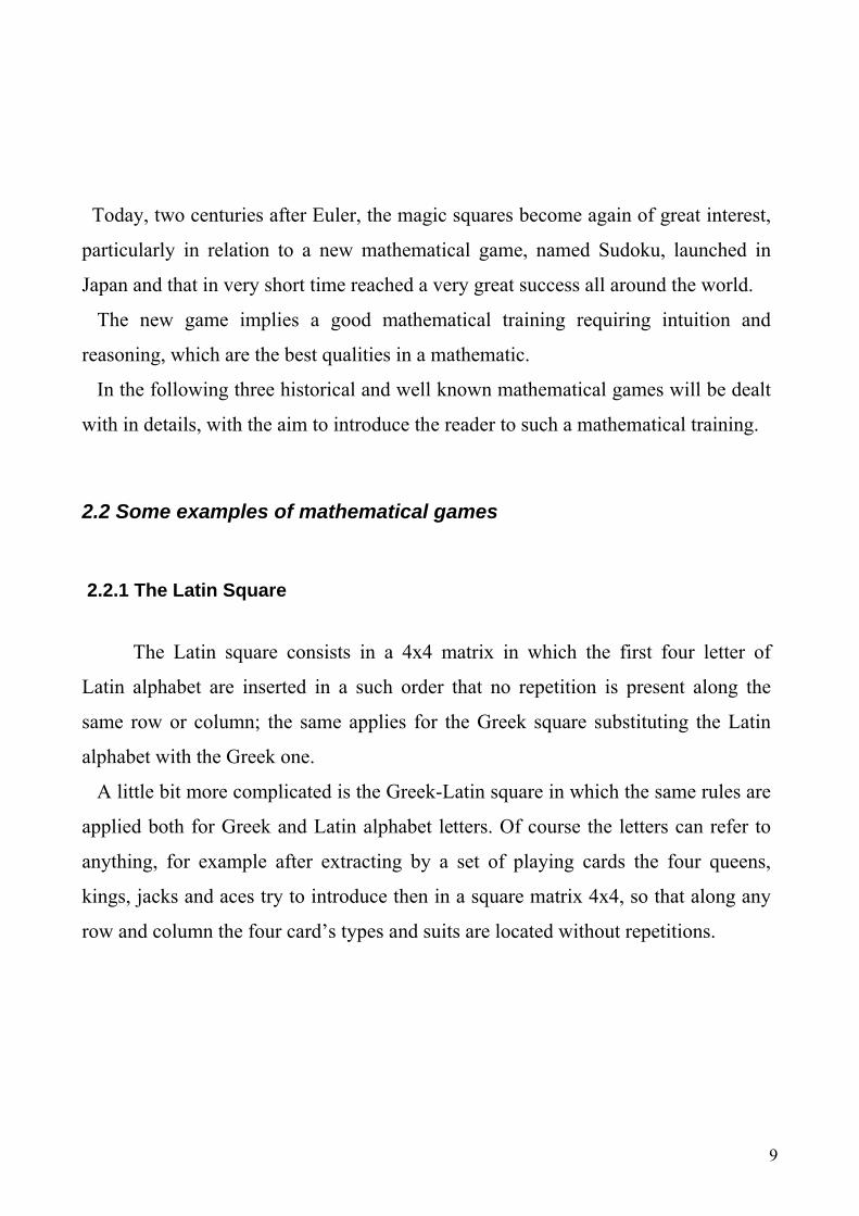
Today, two centuries after Euler, the magic squares become again of great interest,

particularly in relation to a new mathematical game, named Sudoku, launched in

Japan and that in very short time reached a very great success all around the world.

The new game implies a good mathematical training requiring intuition and

reasoning, which are the best qualities in a mathematic.

In the following three historical and well known mathematical games will be dealt

with in details, with the aim to introduce the reader to such a mathematical training.

2.2 Some examples of mathematical games

2.2.1 The Latin Square

The Latin square consists in a 4x4 matrix in which the first four letter of

Latin alphabet are inserted in a such order that no repetition is present along the

same row or column; the same applies for the Greek square substituting the Latin

alphabet with the Greek one.

A little bit more complicated is the Greek-Latin square in which the same rules are

applied both for Greek and Latin alphabet letters. Of course the letters can refer to

anything, for example after extracting by a set of playing cards the four queens,

kings, jacks and aces try to introduce then in a square matrix 4x4, so that along any

row and column the four card’s types and suits are located without repetitions.

10

Fig.4: the “Greek-Latin square”

A classical application of Latin square is in the statistic field, being a system to solve

in a rational way some experimental tests. For instance one can imagine to need to

test five different types of fertilizers for a specific farming. One can scatter the

fertilizer on one field and after the harvest measure the production per unit area; but

in such a way one is obliged to perform the experiment on five different fields, the

proprieties of which can be different. On the opposite if the same field is divided in

5x5 squares on which the fertilizers are applied following the schema of Latin

square, a more correct and complete analysis may be obtained.

11

The complexity of magic squares increases very fast when the fourth order is

exceeded; it is known that 880 different types of magic squares exist, considering the

rotations and the specular images, having also more complex properties with respect

to the elementary ones.

2.2.2 The Rubik’s cube

The Rubik cube has been designed by an Hungarian mathematic and architect,

Erno Rubik, in 1974. The cube consists of 26 smaller cubes inserted in a 3x3x3

matrix coloured in six different colours.

Because it is possible to rotate along its orthogonal axes every set of 9 adjacent

cubes, all the faces of the cube should reach the same uniform colour.

Three years after the invention of Rubik, the cube appeared in the Budapest

shops for mathematical games and have been distributed outside the Hungary in

12

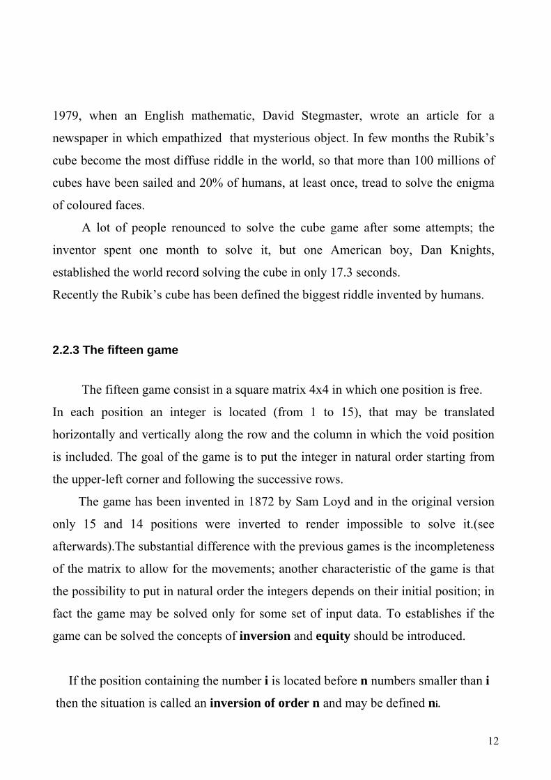
1979, when an English mathematic, David Stegmaster, wrote an article for a

newspaper in which empathized that mysterious object. In few months the Rubik’s

cube become the most diffuse riddle in the world, so that more than 100 millions of

cubes have been sailed and 20% of humans, at least once, tread to solve the enigma

of coloured faces.

A lot of people renounced to solve the cube game after some attempts; the

inventor spent one month to solve it, but one American boy, Dan Knights,

established the world record solving the cube in only 17.3 seconds.

Recently the Rubik’s cube has been defined the biggest riddle invented by humans.

2.2.3 The fifteen game

The fifteen game consist in a square matrix 4x4 in which one position is free.

In each position an integer is located (from 1 to 15), that may be translated

horizontally and vertically along the row and the column in which the void position

is included. The goal of the game is to put the integer in natural order starting from

the upper-left corner and following the successive rows.

The game has been invented in 1872 by Sam Loyd and in the original version

only 15 and 14 positions were inverted to render impossible to solve it.(see

afterwards).The substantial difference with the previous games is the incompleteness

of the matrix to allow for the movements; another characteristic of the game is that

the possibility to put in natural order the integers depends on their initial position; in

fact the game may be solved only for some set of input data. To establishes if the

game can be solved the concepts of inversion and equity should be introduced.

If the position containing the number i is located before n numbers smaller than i

then the situation is called an inversion of order n and may be defined ni.

13

Now one introduces a number of inversion N as :

15 15

1 2i i

i in n

= =

=∑ ∑

where the sums coincide because no integer smaller than 1 is available.

Practically N=i(p) is the number of inversions of permutation of integers

included in the game. N may assume even and odd values.

If N is even the game may be solved; on the opposite, if N is odd the game cannot

be solved.

15

3. THE MATHEMATICAL GAME SUDOKU

3.1 Historical notices about Sudoku

One of the magic square proposed by Euler was a square matrix 9x9 in which

in every row and column the integers from 1 to 9 had to be inserted without any

repetition; that game was practically the progenitor of Sudoku .

After about 200 years a similar game was proposed in New York by Dell, an

editor of a puzzle magazine, with the name of Number Place; this game had a

limited success in U.S. and have been temporally forgotten. In 1984 Nobuliko

Kanemato, an employer of Nikoli publishers, specialized in riddles, revived and

improved this game, patented and proposed it to the people with the name “Suuji wa

dokushin ni Kagiru ( the numbers that should appear only ones ).

Finally in 1997 a New Zeeland retired judge, Wayne Gould, visited Tokyo,

discovered the SUDOKU ( an abbreviation of previous title, where SU stands for

number and DOKU stands for single ) and get crazy for it. He invented and

improved a software for the Sudoku generation and proposed it to the Times of

London, that launched it in November 2004.

This game that today is very successful is characterized by a common parameter:

single is the game, singles are the integers to be included within the matrix, single is

the spare time, which is available to solve the Sudoku. Practically this game may be

considered a serial game like the crosswords but less flexible, because the last one

regenerate himself by means of lexicon and permits thousands of variations and of

difficulty levels; one conclude that in the panorama of mathematical games the

Sudoku may be inserted between crosswords and Rubik’s cube.

16

3.2 Sudoku definition and rules

Sudoku is a riddle apparently simple, but in fact requires a strategy to be

solved; nevertheless it uses numbers it is not a matter of mathematics; in fact

numbers may be submitted by symbols but traditionally numbers are used.

The rules of this game are very simple and only a pencil and a piece of paper is

required to play it. The frame of the game is a matrix 9x9 and in each position an

integer included between 1 and 9 should be inserted. Each row, each column and

every sub-matrix 3x3 should include all the integers between 1 and 9 without

repetitions. A Sudoku game contains some positions fixed by default, so that there

is only one valid solution; the game generator should then consider the necessity to

ensure the uniqueness of the solution by the definition of a set of constrains by

means of fixed integers and their position within the matrix.

Of course the so defined set of restrains in practice may be integrated by further

constrains to facilitate the solution of the game.

17

4. COMPUTATIONAL COMPLEXITY

4.1 Definition of computational complexity

A problem may be considered like a general question to be solved,

characterized

by different parameters, the value of which are not specified. The problem is defined

by :

- a general description of all its parameters

- defining the properties that the solution must satisfy

An instance of a problem is given when some values are specified for the problem

parameters.

One consider, for example, a classical problem of Combinatorial optimization:

The TSP problem (Travelling Salesman Problem ), that is n cities Ai connected by

roads of given relative length.

A commercial traveller should determine an itinerary such that he can visit only

once every city with the minimum overall travel length.

The parameters of such a problem are:

- a finite set of cities C=A1,A2,..An

- for every couple (Ai , Aj ) in C, the distance between Ai and Aj, called

d(Ai , Aj)

A solution of the problem is given by the order < Aπ(1),Aπ(2),…,A π(n) > of cities

that minimizes

Σ d(A π(ι),A π(ι+1)) + d(A π(m),A π(1)) (1)

18

Where (1) expresses the length of run beginning from A π(1) reaching all the

other cities in sequence and coming back to A π(1) from the last city reached

A π(m).

Informally one can say that an algorithm is a step by step procedure bringing to

the problem solution.

An algorithm is able to solve a problem π if it can be applied to whichever

instance of π ensuring always to find a solution.

In the case of TSP an algorithm solves the problem if it is able to individuate a

sequence of cities producing a circuit with minimum length.

Generally the most efficient algorithm is the fastest, assuming as fundamental

variable in defining its efficiency, the time spent to solve the problem.

The time requirements can be expanded as a function of the problem instance,

that is of the entity of input data describing the instance.

The instance may be considered as a single finite strip of symbols chosen

within a finite alphabet; the input length for the instance “I” of a problem “π” is

given by the symbols number contained in the “I” strip; this number represents

the formal measure of the instance. The function “complexity in time” of an

algorithm expresses its time requirements, measuring, for every dimension of the

instance, the time necessary to the algorithm to solve it.

Of course other variables are the codification schema employed and the

capacity of the computer used for the solution of the instance.

19

The complexity of an algorithm is a function of problem instance dimension.

Two different definition of this function are recognized.

Being f the time complexity function associated to an algorithm, in the

dimension of the problem instance and g : N → N one can define:

a) worst case

one say that f(n) € O (g(n)) if n^,c >0 exists so that f(n) ≤c * f(n) , every n ≥

n^

b) best case

one say that f(n) € Ω (g(n)) if n^,c >0 exists so that f(n) ≥ c * f(n) , every n ≥

n^

The case a) is used practically to evaluate the computational complexity of an

algorithm.

An algorithm characterized by a time complexity function O(g(n)), with g(n)

polynomial function of n is named polynomial algorithm; instead are not polynomial

the algorithms where g(n) = 2^n or g(n)=n!

This distinction assumes a great importance when the solution for large instances

of problems is considered. The application of non polynomial algorithms becomes

prohibitive with the increasing of the dimension of the instance: for a very small

value of n a non polynomial algorithm may be faster than a polynomial one, but ,

increasing n, a polynomial algorithm will be always more efficient than the non

polynomial one.

With the technological improvement of computers polynomial algorithms are more

advantaged than the non polynomial ones; in practice if the power of computers

20

increases by a factor γ, the dimension of largest instance solvable by a polynomial

algorithm in a prefixed time is amplified by a constant in the range (1, γ),on the

opposite the increment for a non polynomial algorithm is only additional, in the

dimension of the instance solvable within the predefined time.

4.2 Computational complexity classes

One refers now to the “decisional version” of optimization problems. In the

decisional version of an optimization problem there are only two possible solutions:

the answers yes and not. The standard format used to specify an optimization

problem in its decisional version consists generally of two parts:

- the first part specifies an instance of the problem, assigning the values to the

problem parameters;

- the second part establishes a question related to the instance, for which the

answer yes or not is possible.

One can now introduce a classification of problems in terms of computational

complexity.

- The P Class

The P Class is the set of all problems solvable, in the worst case, by a

polynomial algorithm; the problems of class P are very often defined as

“easy” problem.

- The NP Class

The NP Class (non-deterministic polynomial) is the set of all the decision

problems solvable, in the worst case, by a non-deterministic polynomial.

A such algorithm is an algorithm in which two steps may be recognized:

21

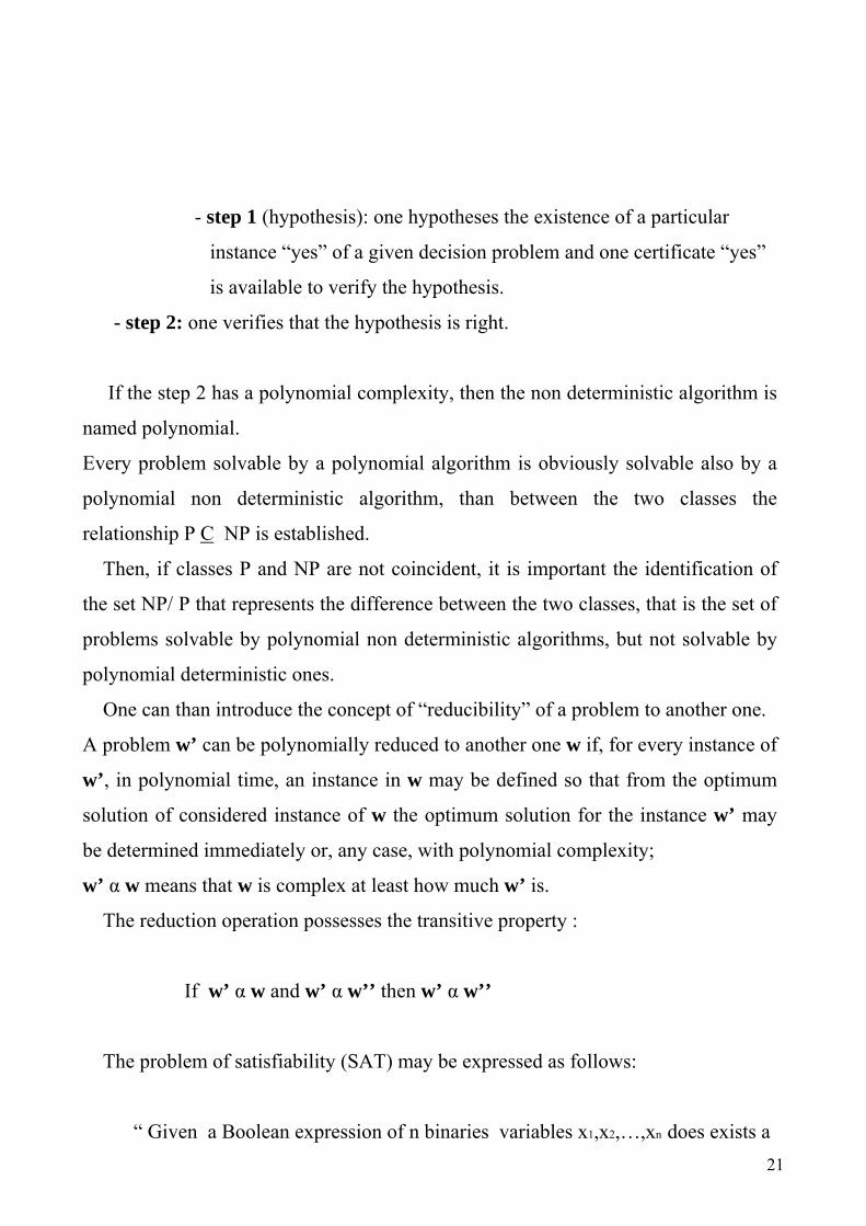
- step 1 (hypothesis): one hypotheses the existence of a particular

instance “yes” of a given decision problem and one certificate “yes”

is available to verify the hypothesis.

- step 2: one verifies that the hypothesis is right.

If the step 2 has a polynomial complexity, then the non deterministic algorithm is

named polynomial.

Every problem solvable by a polynomial algorithm is obviously solvable also by a

polynomial non deterministic algorithm, than between the two classes the

relationship P C NP is established.

Then, if classes P and NP are not coincident, it is important the identification of

the set NP/ P that represents the difference between the two classes, that is the set of

problems solvable by polynomial non deterministic algorithms, but not solvable by

polynomial deterministic ones.

One can than introduce the concept of “reducibility” of a problem to another one.

A problem w’ can be polynomially reduced to another one w if, for every instance of

w’, in polynomial time, an instance in w may be defined so that from the optimum

solution of considered instance of w the optimum solution for the instance w’ may

be determined immediately or, any case, with polynomial complexity;

w’ α w means that w is complex at least how much w’ is.

The reduction operation possesses the transitive property :

If w’ α w and w’ α w’’ then w’ α w’’

The problem of satisfiability (SAT) may be expressed as follows:

“ Given a Boolean expression of n binaries variables x1,x2,…,xn does exists a

22

solution x1’,x2’,…,xn ’ rending right the Boolean expression? ”

The solution is that (Cook theorem) if w € NP, than w α SAT

One can now introduce the NP complete problems, that is the set of all problems

verifying the following two conditions

a) w € NP

b) SAT α w

A typical characteristics of much problems is that all the NP complete problems

have the same level of difficulty.

One consider now a problem w, the appertaining of which to the class NP cannot

be verified, but satisfying the condition E w’ NP complete, so that w’ α w. The

problem NP is then, at least, complex like a NP complete one, but its appertaining to

NP class cannot be ensured : such kind of problem is named NP hard.

Finally some further problems exists, for which neither the appertaining to the

class P or the class NP complete has been demonstrated, nevertheless they appertain

to the NP class.

Such kind of problems are named “open”.

Now other definitions for the algorithms should be introduced:

- An algorithm having polynomial complexity in unary codification and non-

polynomial in binary codification is named NP-complete (NP-hard) in

ordinary mean.

- An optimization problem NP-complete (NP-hard) for which exact algorithms

for polynomial solution does not exists, the operator of which can be confined

23

within a memory space in the computer limited by a polynomial function with

the same dimension of the input, is named P-space.

4.3 Computational complexity of the Sudoku problem

The computational complexity for a Sudoku problem is analytically valuable,

in fact, at every step there is always a cell that can be filled only with a number, than

the complexity results O(n^2),where n is the number of cells for each row or

column,(in our case n=9).

Instead, for a generalized Sudoku problem (a Sudoku problem that has not a

unique solution) the computational complexity is not easily valuable analytically but

may be evaluated by comparison with the corresponding one of a problem, the

mathematical complexity of which has been evaluated and is known.

As reference problem for the computational complexity evaluation, the

“crosswords puzzle construction” problem is taken into consideration.

This game is defined by the following instance and questions:

- INSTANCE : A finite set W C Σ’ of words and an nxn matrix A of 0’s and

1’s.

- QUESTIONS: Can an nxn crosswords puzzle be built up from the words in

W and blank squares corresponding to the 0’s of A, i.e. if E is the set of pairs

(i,j) such that Aij = 0, is there an assignment f: E → Σ such that the letters

assigned to any maximal horizontal or vertical contiguous sequence of

members of E from, in order, a word of W ?

In this comparison the initial schema of Sudoku may be considered as

corresponding to the matrix A of crosswords puzzle construction; similarly a

correspondence is defined between the set E and the set of initial prefixed position of

24

given content in Sudoku and in addition between the set Σ and the set of all position

in Sudoku and between the set W and the set of possible integer strips in Sudoku.

Having so established a correspondence between the two games one can derive

that Sudoku has a computational complexity at least of the same order of magnitude

of “crosswords puzzle construction” problem.

25

5. DEFINITION OF A MATHEMATICAL MODEL ABLE TO DESCRIBE SUDOKU

5.1 Variables in the mathematical models

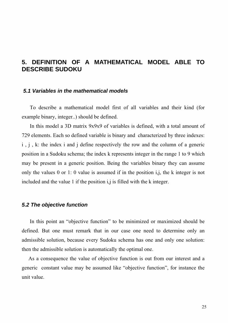
To describe a mathematical model first of all variables and their kind (for

example binary, integer..) should be defined.

In this model a 3D matrix 9x9x9 of variables is defined, with a total amount of

729 elements. Each so defined variable is binary and characterized by three indexes:

i , j , k: the index i and j define respectively the row and the column of a generic

position in a Sudoku schema; the index k represents integer in the range 1 to 9 which

may be present in a generic position. Being the variables binary they can assume

only the values 0 or 1: 0 value is assumed if in the position i,j, the k integer is not

included and the value 1 if the position i,j is filled with the k integer.

5.2 The objective function

In this point an “objective function” to be minimized or maximized should be

defined. But one must remark that in our case one need to determine only an

admissible solution, because every Sudoku schema has one and only one solution:

then the admissible solution is automatically the optimal one.

As a consequence the value of objective function is out from our interest and a

generic constant value may be assumed like “objective function”, for instance the

unit value.

26

5.3 Constraints

The constraints, necessary to limit the field of the problem, are linear

combinations of variables giving a constant value.

The model contains the following typology of constraints:

- having fixed a j column, at the crossing of each row i with the j column, the

sum of variables included within correspondent k column shall assume unit

value;

- within the matrix i,k the sum of variables along i for each k assumes unit

value

- having fixed an i row, at the crossing of each column j with the i row, the sum

of variables included within correspondent k column shall assume unit value;

- within the matrix j,k the sum of variables along i for each k assumes unit

value

- for every sub-matrix 3x3 (i,j) the sum of variables for each k shall assume unit

value;

Of course all the previous constraints define an empty Sudoku schema ; but if we

want to introduce in the schema some predefined values in predefined position,

the corresponding values shall be also predefined assuming the unit value;

nothing to say that such predefined values shall respect the above defined

restraints.

27

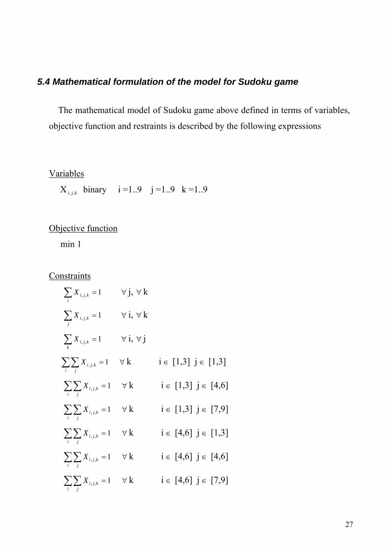
5.4 Mathematical formulation of the model for Sudoku game

The mathematical model of Sudoku game above defined in terms of variables,

objective function and restraints is described by the following expressions

Variables

X kji ,, binary i =1..9 j =1..9 k =1..9

Objective function

min 1

Constraints

1,, =∑i

kjiX ∀ j, ∀ k

1,, =∑j

kjiX ∀ i, ∀ k

1,, =∑k

kjiX ∀ i, ∀ j

1,, =∑∑i j

kjiX ∀ k i ∈ [1,3] j ∈ [1,3]

1,, =∑∑i j

kjiX ∀ k i ∈ [1,3] j ∈ [4,6]

1,, =∑∑i j

kjiX ∀ k i ∈ [1,3] j ∈ [7,9]

1,, =∑∑i j

kjiX ∀ k i ∈ [4,6] j ∈ [1,3]

1,, =∑∑i j

kjiX ∀ k i ∈ [4,6] j ∈ [4,6]

1,, =∑∑i j

kjiX ∀ k i ∈ [4,6] j ∈ [7,9]

28

1,, =∑∑i j

kjiX ∀ k i ∈ [7,9] j ∈ [1,3]

1,, =∑∑i j

kjiX ∀ k i ∈ [7,9] j ∈ [4,6]

1,, =∑∑i j

kjiX ∀ k i ∈ [7,9] j ∈ [7,9]

5.5 Three-dimensional Sudoku

The Sudoku game can be extended to the three-dimensional space.

In this case we will consider a 27x27x27 cube.

To solve our problem we need a variable with four indexes, , , ,i j k tX ,

where the index i,j,k represents the position of the considered cell and the

index t represents the number that can be contained in the cell.

Every index takes integer value in [1,27],so that the number of variables is equal to

531441.

The constraints are like that:

- in each column, in each row and in each vertical column, and in each little

cube

3x3x3, a number must be contained one and only one times.

This problem can be also extended to n-dimensional space, through the same

considerations.

29

6. IMPLEMENTATION OF THE MODEL IN XPRESS SOLVER

The so defined mathematical model describing Sudoku has been implemented

within the frame of XPRESS solver, an optimization software, to render it easily

applicable.

This implementation process require that the expressions presented in chapter

five above are transferred within XPRESS as described below.

6.1 Mathematical model of Sudoku implemented in XPRESS

The following expressions describe the mathematical model Sudoku within

the XPRESS solver.

30

model "sudoku"

uses "mmxprs"

declarations

I=1..9

J=1..9

K=1..9

P=1

x:array(I,J,K)of mpvar

end-declarations

forall(i in I,j in J, k in K) x(i,j,k) is_binary

forall(j in J,k in K) sum(i in I)x(i,j,k)=1

forall(i in I,k in K) sum(j in J)x(i,j,k)=1

forall(i in I,j in J) sum(k in K)x(i,j,k)=1

forall(k in K) sum(i in 1..3,j in 1..3) x(i,j,k)=1



forall(k in K) sum(z in 4..6,j in 1..3) x(z,j,k)=1



forall(k in K) sum(t in 7..9,j in 1..3) x(t,j,k)=1



x(1,2,6)=1

x(1,3,1)=1

x(1,5,3)=1

x(1,8,2)=1

x(2,2,5)=1

x(2,6,8)=1

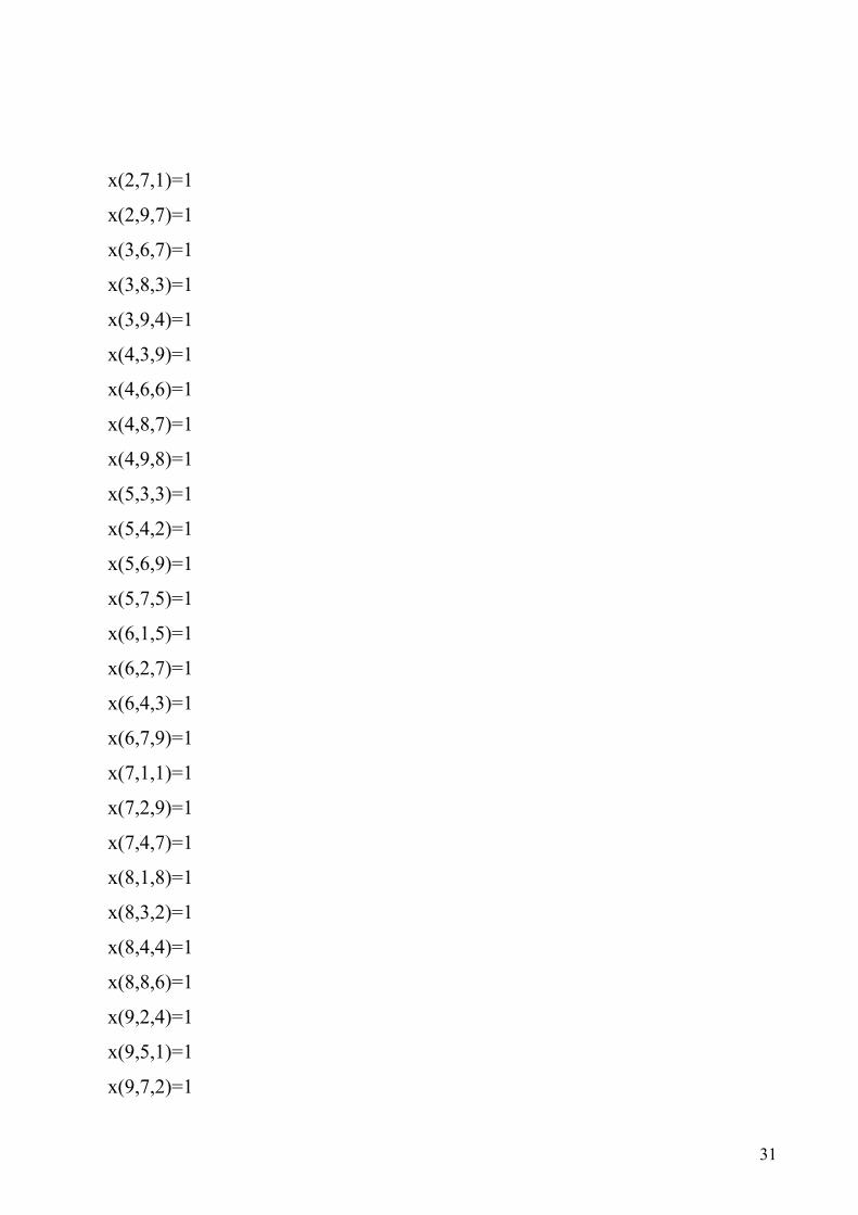
31

x(2,7,1)=1

x(2,9,7)=1

x(3,6,7)=1

x(3,8,3)=1

x(3,9,4)=1

x(4,3,9)=1

x(4,6,6)=1

x(4,8,7)=1

x(4,9,8)=1

x(5,3,3)=1

x(5,4,2)=1

x(5,6,9)=1

x(5,7,5)=1

x(6,1,5)=1

x(6,2,7)=1

x(6,4,3)=1

x(6,7,9)=1

x(7,1,1)=1

x(7,2,9)=1

x(7,4,7)=1

x(8,1,8)=1

x(8,3,2)=1

x(8,4,4)=1

x(8,8,6)=1

x(9,2,4)=1

x(9,5,1)=1

x(9,7,2)=1

32

maximize(1)

forall(i in I) do

forall(j in J, k in K) do

if getsol(x(i,j,k))=1

then

write(k, " ")

end-if

end-do

writeln("")

end-do

end-model

6.2 Instance generation program

To apply practically the Sudoku program implemented in XPRESS an

instance generation program has been written in C++ language; this program is

able to generate a Sudoku game having chosen the number of fixed parameters to

be introduced, the position of which is defined by the program by means of a

random generator; a second program assigns the predefined integers to the

position chosen as above described. In the following pages the instruction of

the programs are reproduced.

# include <stdio.h>

# include <stdlib.h>

# include <time.h>

33

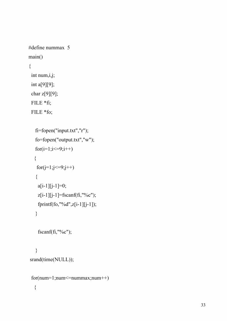
#define nummax 5

main()

int num,i,j;

int a[9][9];

char z[9][9];

FILE *fi;

FILE *fo;

fi=fopen("input.txt","r");

fo=fopen("output.txt","w");

for(i=1;i<=9;i++)

for(j=1;j<=9;j++)

a[i-1][j-1]=0;

z[i-1][j-1]=fscanf(fi,"%c");

fprintf(fo,"%d",z[i-1][j-1]);

fscanf(fi,"%c");

srand(time(NULL));

for(num=1;num<=nummax;num++)

34

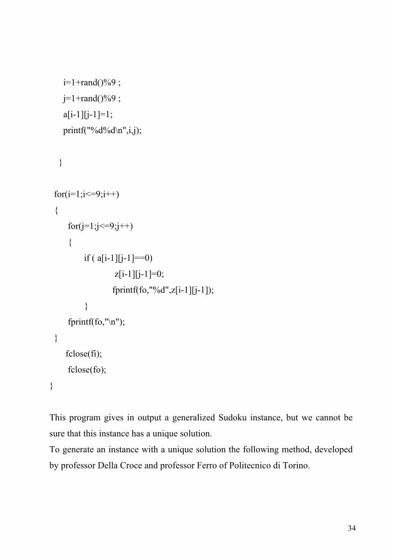
i=1+rand()%9 ;

j=1+rand()%9 ;

a[i-1][j-1]=1;

printf("%d%d\n",i,j);

for(i=1;i<=9;i++)

for(j=1;j<=9;j++)

if ( a[i-1][j-1]==0)

z[i-1][j-1]=0;

fprintf(fo,"%d",z[i-1][j-1]);

fprintf(fo,"\n");

fclose(fi);

fclose(fo);

This program gives in output a generalized Sudoku instance, but we cannot be

sure that this instance has a unique solution.

To generate an instance with a unique solution the following method, developed

by professor Della Croce and professor Ferro of Politecnico di Torino.

35

Suppose that the model presented above has been solved and a feasible solution

has been found. Denote by SOL(i,j) the value of the element (i,j) of the schema

in the feasible solution. Solve the following model P2:

Variables:

The same used in the previous model

Objective function :

min z =, , : ( , ) ijki j k SOL i j k

X=∑

Constraints:

1,, =∑i

kjiX ∀ j, ∀ k

1,, =∑j

kjiX ∀ i, ∀ k

1,, =∑k

kjiX ∀ i, ∀ j

1,, =∑∑i j

kjiX ∀ k i ∈ [1,3] j ∈ [1,3]

1,, =∑∑i j

kjiX ∀ k i ∈ [1,3] j ∈ [4,6]

1,, =∑∑i j

kjiX ∀ k i ∈ [1,3] j ∈ [7,9]

1,, =∑∑i j

kjiX ∀ k i ∈ [4,6] j ∈ [1,3]

1,, =∑∑i j

kjiX ∀ k i ∈ [4,6] j ∈ [4,6]

1,, =∑∑i j

kjiX ∀ k i ∈ [4,6] j ∈ [7,9]

1,, =∑∑i j

kjiX ∀ k i ∈ [7,9] j ∈ [1,3]

1,, =∑∑i j

kjiX ∀ k i ∈ [7,9] j ∈ [4,6]

1,, =∑∑i j

kjiX ∀ k i ∈ [7,9] j ∈ [7,9]

36

The solution of this model provides a feasible solution also to the previous

model.

The objective function of model P2 minimizes the sum of the elements in the grid

having the same value obtained in the solution of the previous model. Hence , as

each grid is composed by 81 elements, if the objective function value of model

P2 is equal to 81 (Z=81), then the Sudoku problem has unique solution, else it

has not.

37

7. APPLICATIONS AND EXPERIMENTAL RESULTS

In this chapter some examples of Sudoku instance on which our model has

been tested will be given.

The following examples are divided in four different categories based on the

difficulty level: easy, medium, difficult and diabolic.

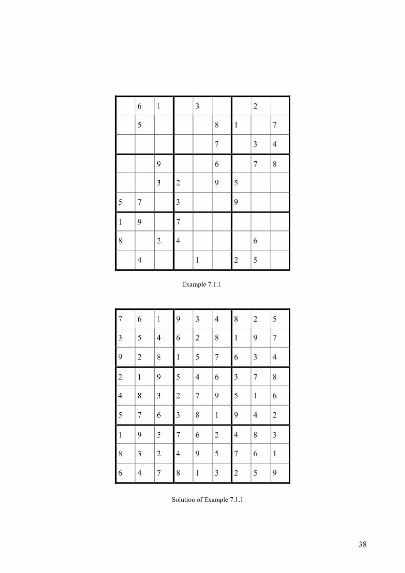
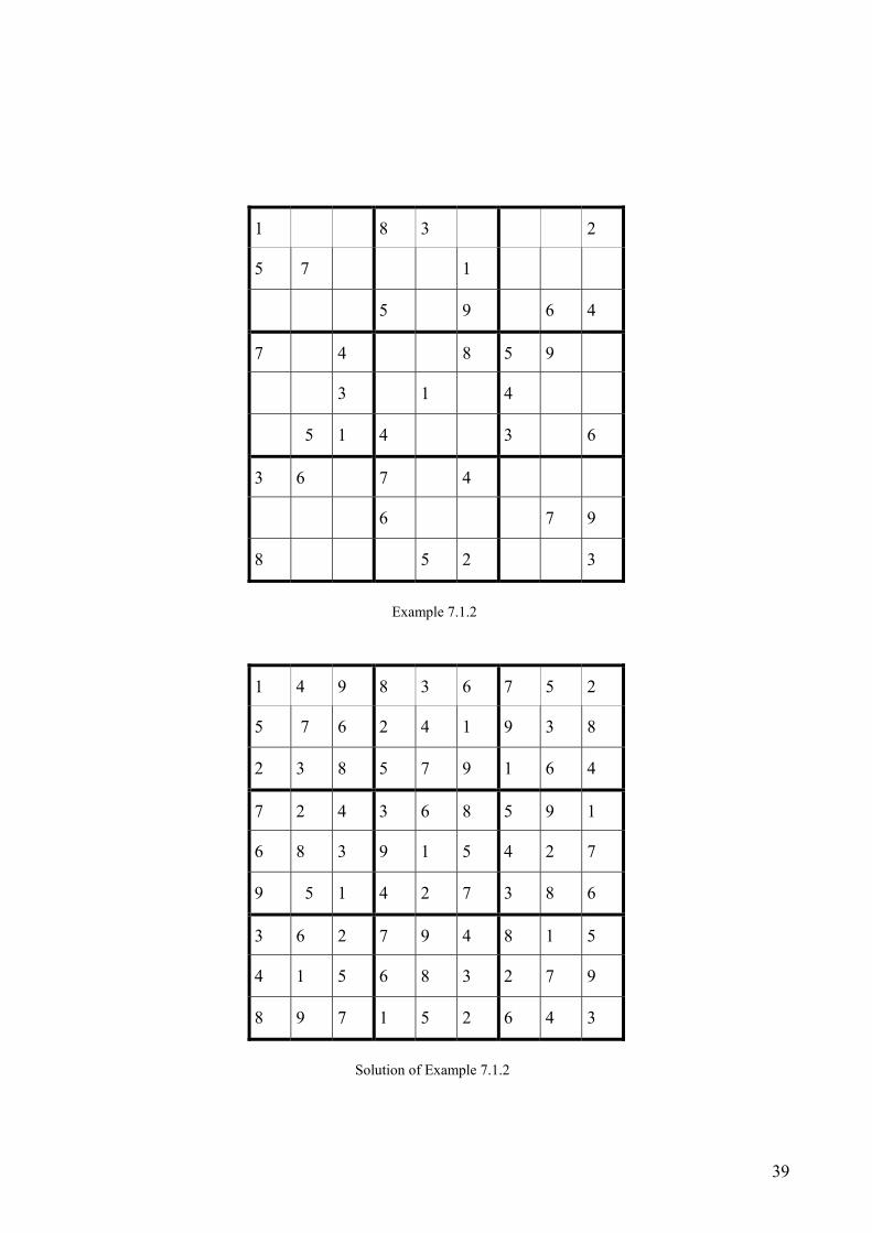
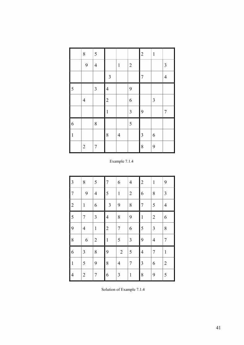
7.1 Easy instances

These instances are characterized by a very big number of prefixed values,

about 34-35 cells, distributed homogeneously on the grid. It is very simple to

solve them; therefore they are designed for people that approach Sudoku for the

first time. Here some examples of this kind of instances are reported.

38

6 1 3 2

5 8 1 7

7 3 4

9 6 7 8

3 2 9 5

5 7 3 9

1 9 7

8 2 4 6

4 1 2 5

Example 7.1.1

7 6 1 9 3 4 8 2 5

3 5 4 6 2 8 1 9 7

9 2 8 1 5 7 6 3 4

2 1 9 5 4 6 3 7 8

4 8 3 2 7 9 5 1 6

5 7 6 3 8 1 9 4 2

1 9 5 7 6 2 4 8 3

8 3 2 4 9 5 7 6 1

6 4 7 8 1 3 2 5 9

Solution of Example 7.1.1

39

1 8 3 2

5 7 1

5 9 6 4

7 4 8 5 9

3 1 4

5 1 4 3 6

3 6 7 4

6 7 9

8 5 2 3

Example 7.1.2

1 4 9 8 3 6 7 5 2

5 7 6 2 4 1 9 3 8

2 3 8 5 7 9 1 6 4

7 2 4 3 6 8 5 9 1

6 8 3 9 1 5 4 2 7

9 5 1 4 2 7 3 8 6

3 6 2 7 9 4 8 1 5

4 1 5 6 8 3 2 7 9

8 9 7 1 5 2 6 4 3


40

3 7 4

6 2 4 1

3 9 6 7

4 3 6

8 7 3 5

9 7 2

7 1 8 2 4

1 6 8 9

4 5 3

Example 7.1.3

8 3 9 6 5 7 2 1 4

6 7 2 9 4 1 5 8 3

1 5 4 8 3 2 9 6 7

5 4 1 2 8 3 7 9 6

2 8 7 4 9 6 3 5 1

9 6 3 7 1 5 4 2 8

7 1 8 3 2 9 6 4 5

3 2 5 1 6 4 8 7 9

4 9 6 5 7 8 1 3 2


41

8 5 2 1

9 4 1 2 3

3 7 4

5 3 4 9

4 2 6 3

1 3 9 7

6 8 5

1 8 4 3 6

2 7 8 9

Example 7.1.4

3 8 5 7 6 4 2 1 9

7 9 4 5 1 2 6 8 3

2 1 6 3 9 8 7 5 4

5 7 3 4 8 9 1 2 6

9 4 1 2 7 6 5 3 8

8 6 2 1 5 3 9 4 7

6 3 8 9 2 5 4 7 1

1 5 9 8 4 7 3 6 2

4 2 7 6 3 1 8 9 5


42

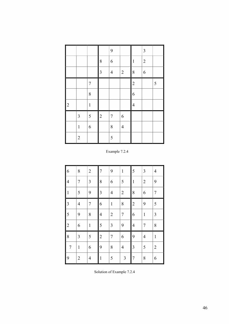
7.2 Medium instances

These instances are a bit more complicated than the previous ones. The number

of prefixed values is about 30, but the great difference with respect to the easy

instances is the position of these values. In fact, in an easy scheme there are

always at least three fixed elements for each row, column and sub-matrix,

while in the medium cases is possible to have two column or rows (see example

7.2.2 and 7.2.3), or three sub-matrix, completely empty (see example 7.2.4).

43

9 4 5

6

5 2 1 3 8 7

9 3 1

3 8 1

4 6 2

7 5 2 8 1 9

3

8 6 1

Example 7.2.1

3 1 8 6 2 7 9 4 5

9 7 6 8 5 4 2 3 1

5 2 4 1 9 3 8 6 7

4 9 2 3 1 5 6 7 8

6 5 3 7 8 2 1 9 4

1 8 7 9 4 6 5 2 3

7 3 5 2 6 8 4 1 9

2 4 9 5 7 1 3 8 6

8 6 1 4 3 9 7 5 2


44

4 7 1 8 2 9

6 9 2 7 1

9 6 1 3

3 4

4 7 9 8

4 8 7 5 3

5 8 4 3 9 7

Example 7.2.2

4 7 3 1 6 8 5 2 9

1 2 9 3 5 4 8 7 6

8 5 6 9 2 7 1 4 3

2 9 8 6 4 1 7 3 5

3 1 7 5 8 2 9 6 4

6 4 5 7 3 9 2 8 1

9 6 4 8 7 5 3 1 2

7 3 1 2 9 6 4 5 8

5 8 2 4 1 3 6 9 7


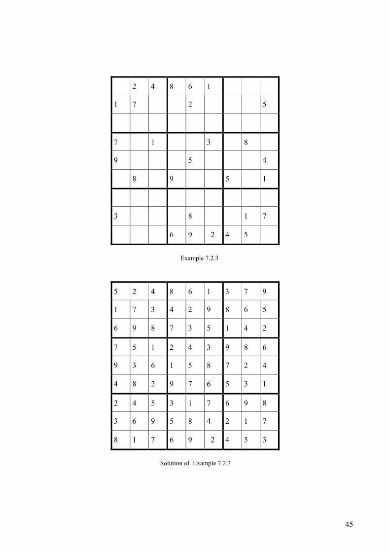
45

2 4 8 6 1

1 7 2 5

7 1 3 8

9 5 4

8 9 5 1

3 8 1 7

6 9 2 4 5

Example 7.2.3

5 2 4 8 6 1 3 7 9

1 7 3 4 2 9 8 6 5

6 9 8 7 3 5 1 4 2

7 5 1 2 4 3 9 8 6

9 3 6 1 5 8 7 2 4

4 8 2 9 7 6 5 3 1

2 4 5 3 1 7 6 9 8

3 6 9 5 8 4 2 1 7

8 1 7 6 9 2 4 5 3


46

9 3

8 6 1 2

3 4 2 8 6

7 2 5

8 6

2 1 4

3 5 2 7 6

1 6 8 4

2 5

Example 7.2.4

6 8 2 7 9 1 5 3 4

4 7 3 8 6 5 1 2 9

1 5 9 3 4 2 8 6 7

3 4 7 6 1 8 2 9 5

5 9 8 4 2 7 6 1 3

2 6 1 5 3 9 4 7 8

8 3 5 2 7 6 9 4 1

7 1 6 9 8 4 3 5 2

9 2 4 1 5 3 7 8 6


47

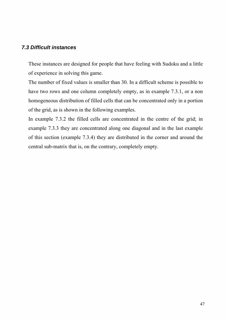
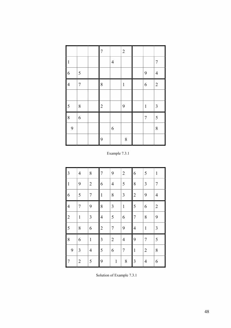
7.3 Difficult instances

These instances are designed for people that have feeling with Sudoku and a little

of experience in solving this game.

The number of fixed values is smaller than 30. In a difficult scheme is possible to

have two rows and one column completely empty, as in example 7.3.1, or a non

homogeneous distribution of filled cells that can be concentrated only in a portion

of the grid, as is shown in the following examples.

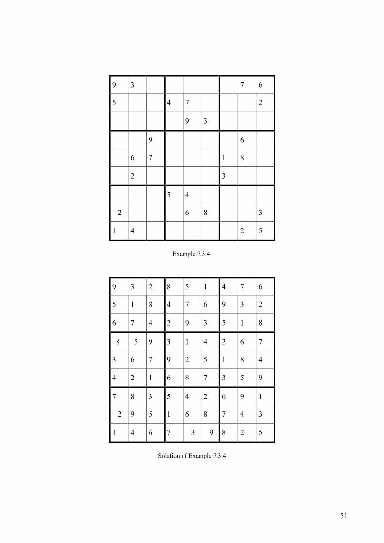
In example 7.3.2 the filled cells are concentrated in the centre of the grid; in

example 7.3.3 they are concentrated along one diagonal and in the last example

of this section (example 7.3.4) they are distributed in the corner and around the

central sub-matrix that is, on the contrary, completely empty.

48

7 2

1 4 7

6 5 9 4

4 7 8 1 6 2

5 8 2 9 1 3

8 6 7 5

9 6 8

9 8

Example 7.3.1

3 4 8 7 9 2 6 5 1

1 9 2 6 4 5 8 3 7

6 5 7 1 8 3 2 9 4

4 7 9 8 3 1 5 6 2

2 1 3 4 5 6 7 8 9

5 8 6 2 7 9 4 1 3

8 6 1 3 2 4 9 7 5

9 3 4 5 6 7 1 2 8

7 2 5 9 1 8 3 4 6


49

5 1 3 7

8 6

6 4

3 9 6 1

8 5 3 9

7 2 8 6

1 3

2 3

9 7 8 1

Example 7.3.2

5 6 1 2 3 4 9 8 7

3 8 4 1 9 7 5 6 2

7 9 2 8 5 6 3 1 4

2 5 3 9 6 1 4 7 8

8 7 6 5 4 3 1 2 9

4 1 9 7 2 8 6 5 3

1 4 7 3 8 5 2 9 6

6 2 8 4 1 9 7 3 5

9 3 5 6 7 2 8 4 1


50

7 1 5 4

9 1

5 8 6

4 6 8

1 4 3

3 9 2

2 6 1

3 2

5 7 2 8

Example 7.3.3

7 6 3 9 1 2 8 5 4

8 9 4 3 6 5 2 7 1

2 1 5 8 7 4 3 6 9

4 3 2 6 8 1 7 9 5

1 5 9 2 4 7 6 8 3

6 8 7 5 3 9 4 1 2

9 2 8 4 5 6 1 3 7

3 4 1 7 9 8 5 2 6

5 7 6 1 2 3 9 4 8


51

9 3 7 6

5 4 7 2

9 3

9 6

6 7 1 8

2 3

5 4

2 6 8 3

1 4 2 5

Example 7.3.4

9 3 2 8 5 1 4 7 6

5 1 8 4 7 6 9 3 2

6 7 4 2 9 3 5 1 8

8 5 9 3 1 4 2 6 7

3 6 7 9 2 5 1 8 4

4 2 1 6 8 7 3 5 9

7 8 3 5 4 2 6 9 1

2 9 5 1 6 8 7 4 3

1 4 6 7 3 9 8 2 5


52

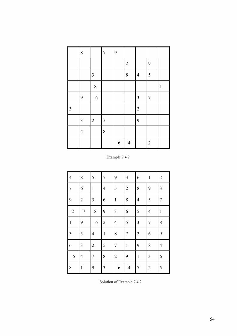
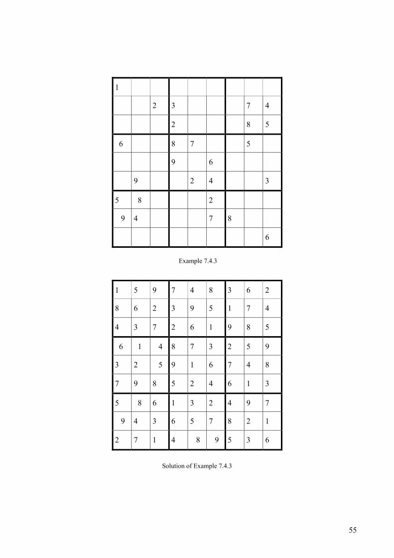
7.4 Diabolic instances

These instances are designed for very expert Sudoku solver. It is very hard to

solve them because the number of prefixed values is smaller than 25 (in some

cases is equal to 22). The above considerations about the distribution of fixed

cells are also valid for these categories of instances. In the follow some examples

of diabolic scheme are reported. In the last example the distribution of the filled

cells is quite homogeneously, but they are only 22, therefore that schema is very

hard to solve. The more difficult scheme that have been solved has only 17 filled

cells but, there is not yet demonstrated that 17 is the minimum number of

prefixed values to guarantee the uniqueness of the solution.

53

8 9 2

9 5 7

5 3

9 3 5 1

1 7

1 6 8 4

8 6

9 6 4

1 2 8

Example 7.4.1

1 6 7 8 9 3 5 2 4

3 4 9 2 1 5 6 8 7

8 5 2 7 6 4 3 1 9

4 9 3 5 8 2 1 7 6

2 8 6 1 4 7 9 5 3

5 7 1 9 3 6 8 4 2

7 3 8 4 5 9 2 6 1

9 2 5 6 7 1 4 3 8

6 1 4 3 2 8 7 9 5


54

8 7 9

2 9

3 8 4 5

8 1

9 6 3 7

3 2

3 2 5 9

4 8

6 4 2

Example 7.4.2

4 8 5 7 9 3 6 1 2

7 6 1 4 5 2 8 9 3

9 2 3 6 1 8 4 5 7

2 7 8 9 3 6 5 4 1

1 9 6 2 4 5 3 7 8

3 5 4 1 8 7 2 6 9

6 3 2 5 7 1 9 8 4

5 4 7 8 2 9 1 3 6

8 1 9 3 6 4 7 2 5


55

1

2 3 7 4

2 8 5

6 8 7 5

9 6

9 2 4 3

5 8 2

9 4 7 8

6

Example 7.4.3

1 5 9 7 4 8 3 6 2

8 6 2 3 9 5 1 7 4

4 3 7 2 6 1 9 8 5

6 1 4 8 7 3 2 5 9

3 2 5 9 1 6 7 4 8

7 9 8 5 2 4 6 1 3

5 8 6 1 3 2 4 9 7

9 4 3 6 5 7 8 2 1

2 7 1 4 8 9 5 3 6


56

3 1 4

9

2 9 3

1 2 7

3 8

8 6 1

1 4 2

5

4 7 8

Example 7.4.4

3 9 5 1 7 2 6 8 4

7 8 1 3 6 4 5 9 2

6 4 2 8 5 9 1 3 7

1 6 4 2 3 8 7 5 9

9 2 3 7 1 5 8 4 6

5 7 8 9 4 6 3 2 1

8 1 7 4 9 3 2 6 5

2 5 9 6 8 1 4 7 3

4 3 6 5 2 7 9 1 8


57

7.5 Computational time

Our model is very efficient, because it is able to solve every Sudoku instance

in a very short time; it takes 0.2 seconds for easy and medium instances, 0.3

seconds for difficult instances and 0.5 seconds for the diabolic ones.

This fact shows that the different difficulty between two levels affects the

performance of an human solver but not that of the program.

7.6 Three-dimensional problems

The model of the three-dimensional problem can not be implemented because

it implies the use of a number of variables bigger than the number of variables

supported by the utilized solver, therefore we have not experimental results for this

problem.

59

8. CONCLUSIONS AND FUTURE DEVELOPMENTS

The Sudoku mathematical game, born about two centuries ago, but largely

spread in Europe only during the last months, has been studied and analysed in

details in this report.

A mathematical model has been formulated. In addition, the mathematical

model has been implemented in a computer solver and in parallel a program has

been developed able to generate Sudoku games. Some application of this

analytical and numerical work have been presented too.

Finally the problem of mathematical complexity has been dealt with, by the

comparison with another game for which the complexity level is known. It has

been also shown that Sudoku has a level of complexity not smaller than the one

of “crossword puzzle construction”.

Further developments in this field should consider the uniqueness of solution in

relation to the minimum number of input data necessary for this condition.

61

Bibliography

- F. Della Croce, G. Ferro, I love Sudoku, Mondatori, Torino, 2006.

- R. Tadei, F. Della Croce, Ricerca operativa e ottimizzazione, Progetto

Leonardo, Esculapio, Bologna, 2002.

- sito web: www.ams.org

- sito web: www.nonzero.it

- sito web: www.nikoli.co

- sito web: www2.polito.it/didattica/polymath

tesi di laurea - polito

Documents