OBSERVATIONAL AND NUMERICAL MODELING STUDIES OF

TURBULENCE ON THE TEXAS-LOUISIANA CONTINENTAL SHELF

A Dissertation

by

ZHENG ZHANG

Submitted to the Office of Graduate Studies ofTexas A&M University

in partial fulfillment of the requirements for the degree of

DOCTOR OF PHILOSOPHY

Chair of Committee, Ayal AnisCo-Chair of Committee, Dongliang ZhaoCommittee Members, Douglas J. Klein

Achim StoesselHead of Department, Piers Chapman

August 2013

Major Subject: Oceanography

Copyright 2013 Zheng Zhang

ABSTRACT

Turbulent dynamics at two sites (C and D) in a hypoxic zone on the Texas-

Louisiana continental shelf were studied by investigating turbulence quantities i.e.

turbulence kinetic energy (TKE), dissipation rate of TKE (ε), Reynolds stress (τ),

dissipation rate of temperature variance (χ), eddy diffusivity of temperature (ν ′t),

and eddy diffusivity of density (ν ′ρ). Numerical models were also applied to test their

capability of simulating these turbulence quantities.

At site D, TKE, ε, and τ were calculated from velocity measurements in the bot-

tom boundary layer (BBL), using the Kolmogorov’s -5/3 law in the inertial subrange

of energy spectra of vertical velocity fluctuations in each burst measurement. Four

second-moment turbulence closure models were applied for turbulence simulations,

and modeled turbulence quantities were found to be consistent with those observed.

It was found from inter-model comparisons that models with the stability functions

of Schumann and Gerz predicted higher values of turbulence quantities than those

of Cheng in the mid layer, which might be due to that the former stability functions

are not sensitive to buoyancy.

At site C, χ, ε, ν ′t, and ν ′ρ were calculated from profile measurements throughout

the water column, and showed high turbulence level in the surface boundary layer

and BBL, as well as in the mid layer where shear stress was induced by advected

non-local water above a hypoxic layer. The relatively high dissolved oxygen in the

non-local water resulted in upward and downward turbulent oxygen fluxes, and the

bottom hypoxia will deform due to turbulence in 7.11 days. Two of the four models

in the study at site D were implemented, and results showed that turbulence energy

resulting from the non-local water was not well reproduced. We attribute this to the

ii

lack of high-resolution velocity measurements for simulations. Model results agreed

with observations only for χ and ε simulated from the model with the stability func-

tion of Cheng in the BBL. Discrepancies between model and observational results

lead to the following conclusions: 1) the stability functions of Schumann and Gerz

are too simple to represent the turbulent dynamics in stratified mid layers; 2) de-

tailed velocity profiles measurements are required for models to accurately predict

turbulence quantities. Missing such observations would result in underestimation,

especially in the mid layer.

iii

DEDICATION

To my Lord, Jesus Christ.

The Lord is my strength and my shield; my heart trusts in him, and he helps me.

My heart leaps for joy, and with my song I praise him. (Psalm 28:7)

iv

ACKNOWLEDGEMENTS

First and foremost, I would like to appreciate my committee chair, Dr. Ayal Anis,

for his expert guidance, patience, encouragement, generosity, and love throughout my

research and my life here. I would like to thank my co-chair Dr. Zhao Dongliang,

and committee members, Dr. Robert D. Hetland, Dr. Douglas J. Klein, and Dr.

Achim Stoessel, for their advices and guidance throughout the course of this research.

Thanks also go to Dr. Alejandro Orsi who were so kind to help me out as the

substitute for Dr. Achim Stoessel, even though the request was sent to him at a very

late time before my defense.

I express my gratitude to Fahad Al Senafi as my comrade everyday, Josh R.

Williams and Dr. Guan-hong Lee for manuscript reviews, Zhang Zhaoru for model

simulations, Li Bo for explanations of hypoxia, Dr. Lars Umlauf and the GOTM user

group for model parameterizations, Edmund Tedford from University of California,

Santa Barbara for SCAMP toolbox and data analysis, Zhao Yan and Dr. Jiang Yuelu

for biology-related discussions, Dr. Xu Chen, Dr. Zhang Saijin, Dr. Hsiu-Ping Li,

Sherry Parker, and Herminia Sandoval for their constant care and encouragement, my

friends Arjun Adhikari, Joseph A. Carlin, Mohammad Al-Mukaimi, Jessica DiGiulio,

Michael Evans, Qu Fangyuan, Yang Chunxue, Li Xinxin, and Xu Zhao for having

wonderful times with them, and Mrs. Ruthy Anis for her lovely baking over the

years.

I would like to thank the NOAA Center for Sponsored Coastal Ocean Research

(NA03NOS4780039 and NA06NOS4780198) for funding this research, Texas A&M

University at Galveston for financial support as Teaching Assistantship, and the

China Scholarship Council for 4-year stipend.

v

I am greatly indebted to my mother Ji Chunhua, my father Zhang Yongjun, my

grandmother Yang Shuying, my aunt Zhang Yongjie, my uncle-in-law Han Shuzong,

and my “brother” Khoi.

Finally, special thanks are given to all the people at the Galveston Chinese

Church. I love you all, and God bless you all.

vi

NOMENCLATURE

ADCP Acoustic Doppler Current Profiler

ADV Acoustic Doppler Velocimeter

BBL Bottom Boundary Layer

CH the k − ε turbulence closure with the stability functions ofCheng et al. (2002)

CHx the k − kL turbulence closure with the stability functions ofCheng et al. (2002)

CTD Conductivity, Temperature, Depth sensor

DO Dissolved Oxygen

DOc critical Dissolved Oxygen

GOTM General Ocean Turbulence Model

HOBO Onset R© U22-001 water temperature logger

NCEP National Centers for Environmental Prediction/Departmentof Energy Reanalysis 2

McFaddin US Forest Service weather station

MCH Mechanisms Controlling Hypoxia

NDBC 42035 National Data Buoy Center station 42035

NDBC LUML1 National Data Buoy Center station LUML1

NOAA National Oceanic and Atmospheric Administration

PIV Particle Image Velocimetry

SBL Surface Boundary Layer

SCAMP Self Contained Autonomous MicroProfiler

SG the k − kL turbulence closure with the stability functions ofSchumann and Gerz (1995)

vii

SGx the k − ε turbulence closure with the stability functions ofSchumann and Gerz (1995)

SST Sea Surface Temperature

TKE Turbulence Kinetic Energy

B buoyancy production

CD drag coefficient

cp heat capacity of water

cµ, c′µ stability functions

db distance from the bottom

ds distance from the sea surface

Dij anisotropic shear production

E energy spectrum

En instrumental noise spectrum

Eobs observed spectrum

f frequency

F wall function

g gravitational acceleration

h water depth

hO2 layer thickness

Hs significant wave height

I solar radiation

J0q net surface heat flux

J lq latent heat flux

J lwq net longwave radiation

Jsq sensible heat flux

Jswq net shortwave radiation

k turbulence kinetic energy

viii

kB Batchelor cutoff wavenumber

kwn radian wavenumber

kwn cyclic wavenumber

L length scale

l0 height of the ADV’s sampling volume above the bottom

M shear frequency

N buoyancy frequency

p pressure

P shear production

Prt turbulent Prandtl number

Ri gradient Richardson number

Rci critical gradient Richardson number

RMAX maximal vertical range of valid ADCP measurement

S salinity

Sij mean shear

t wave period

tO2 time required to remove bottom hypoxia

T temperature

u velocity in the X direction

U mean horizontal current speed

u∞ free-stream mean velocity

Ur mean wind speed at a reference height

v velocity in the Y direction

V horizontal mean current

Vij mean vorticity

w velocity in the Z direction

W falling speed of profiler

ix

z vertical distance

α Kolmogorov constant

βV Ratios of σ to burst-averaged current speed

Γ sum of the viscous and turbulent transport terms

δ mean wave direction

δij Kronecker symbol

δz thickness of the BBL

ε dissipation rate of turbulence kinetic energy

εijl alternating tensor

θ potential temperature

κ von Karman constant,

µ dynamic viscosity

ν kinematic viscosity

νS haline diffusivity

νt eddy viscosity

νT thermal diffusivity

ν ′t eddy diffusivity of temperature

ν ′ρ eddy diffusivity of density

Πij pressure-velocity correlator

ΠiT pressure-temperature correlator

ρ potential density

ρ0 mean density

ρa air density

σ surface-wave-induced orbital velocity

τ Reynold stress

τR relaxation time

τwind wind stress

x

χ dissipation rate of temperature variance

φ angle between wave and current

Ω rotation rate of the earth

xi

TABLE OF CONTENTS

Page

ABSTRACT . . . . . . . . . . . . . . . . . . . . . . . . . . . . . . . . . . . . ii

DEDICATION . . . . . . . . . . . . . . . . . . . . . . . . . . . . . . . . . . . iv

ACKNOWLEDGEMENTS . . . . . . . . . . . . . . . . . . . . . . . . . . . . v

NOMENCLATURE . . . . . . . . . . . . . . . . . . . . . . . . . . . . . . . . vii

TABLE OF CONTENTS . . . . . . . . . . . . . . . . . . . . . . . . . . . . . xii

LIST OF FIGURES . . . . . . . . . . . . . . . . . . . . . . . . . . . . . . . . xiv

LIST OF TABLES . . . . . . . . . . . . . . . . . . . . . . . . . . . . . . . . . xix

1. INTRODUCTION . . . . . . . . . . . . . . . . . . . . . . . . . . . . . . . 1

1.1 Background . . . . . . . . . . . . . . . . . . . . . . . . . . . . . . . . 11.2 Objectives . . . . . . . . . . . . . . . . . . . . . . . . . . . . . . . . . 51.3 Study sites . . . . . . . . . . . . . . . . . . . . . . . . . . . . . . . . . 71.4 Instrumentation . . . . . . . . . . . . . . . . . . . . . . . . . . . . . . 8

1.4.1 General types of instruments for turbulence measurements . . 81.4.2 Instruments used in this research . . . . . . . . . . . . . . . . 10

1.5 Observational analytical methods . . . . . . . . . . . . . . . . . . . . 131.6 Turbulence numerical models . . . . . . . . . . . . . . . . . . . . . . 17

1.6.1 Types of numerical models . . . . . . . . . . . . . . . . . . . . 171.6.2 The general ocean turbulence model . . . . . . . . . . . . . . 24

2. OBSERVATIONS AND MODEL SIMULATIONS OF TURBULENCE INTHE BOTTOM BOUNDARY LAYER OF THE TEXAS-LOUISIANACONTINENTAL SHELF . . . . . . . . . . . . . . . . . . . . . . . . . . . 26

2.1 Introduction . . . . . . . . . . . . . . . . . . . . . . . . . . . . . . . . 262.2 Study site and instrumentation . . . . . . . . . . . . . . . . . . . . . 292.3 Observational approach . . . . . . . . . . . . . . . . . . . . . . . . . . 342.4 Numerical modeling approach . . . . . . . . . . . . . . . . . . . . . . 40

2.4.1 Surface meteorology . . . . . . . . . . . . . . . . . . . . . . . 402.4.2 Hydrography . . . . . . . . . . . . . . . . . . . . . . . . . . . 422.4.3 Model formulation . . . . . . . . . . . . . . . . . . . . . . . . 49

2.5 Analysis . . . . . . . . . . . . . . . . . . . . . . . . . . . . . . . . . . 522.5.1 Observation-model comparisons in the BBL . . . . . . . . . . 53

xii

2.5.2 Inter-model comparisons throughout the water column . . . . 562.5.3 Influence of surface fluxes on turbulence in the BBL . . . . . . 60

2.6 Discussion . . . . . . . . . . . . . . . . . . . . . . . . . . . . . . . . . 612.7 Conclusions . . . . . . . . . . . . . . . . . . . . . . . . . . . . . . . . 62

3. OBSERVATIONS AND MODEL SIMULATIONS OF TURBULENCE INA HYPOXIC ZONE WITH THE ADVECTION OF NON-LOCAL WATER 65

3.1 Introduction . . . . . . . . . . . . . . . . . . . . . . . . . . . . . . . . 653.2 Experimental details . . . . . . . . . . . . . . . . . . . . . . . . . . . 67

3.2.1 Study site . . . . . . . . . . . . . . . . . . . . . . . . . . . . . 673.2.2 Surface forcing . . . . . . . . . . . . . . . . . . . . . . . . . . 673.2.3 Hydrography . . . . . . . . . . . . . . . . . . . . . . . . . . . 703.2.4 Hypoxia and advection . . . . . . . . . . . . . . . . . . . . . . 75

3.3 Observational methods . . . . . . . . . . . . . . . . . . . . . . . . . . 763.4 Turbulent oxygen flux . . . . . . . . . . . . . . . . . . . . . . . . . . 793.5 Model methods . . . . . . . . . . . . . . . . . . . . . . . . . . . . . . 803.6 Comparison between observational and model results . . . . . . . . . 82

3.6.1 χ and ε . . . . . . . . . . . . . . . . . . . . . . . . . . . . . . 823.6.2 ν ′t and ν ′ρ . . . . . . . . . . . . . . . . . . . . . . . . . . . . . . 89

3.7 Discussion . . . . . . . . . . . . . . . . . . . . . . . . . . . . . . . . . 923.8 Conclusions . . . . . . . . . . . . . . . . . . . . . . . . . . . . . . . . 93

4. CONCLUSIONS . . . . . . . . . . . . . . . . . . . . . . . . . . . . . . . . 96

REFERENCES . . . . . . . . . . . . . . . . . . . . . . . . . . . . . . . . . . . 99

APPENDIX A . . . . . . . . . . . . . . . . . . . . . . . . . . . . . . . . . . . 120

APPENDIX B . . . . . . . . . . . . . . . . . . . . . . . . . . . . . . . . . . . 122

APPENDIX C . . . . . . . . . . . . . . . . . . . . . . . . . . . . . . . . . . . 123

xiii

LIST OF FIGURES

FIGURE Page

1.1 Net surface heat flux (J0q ) consists of net flux of solar energy into

the sea (Jswq ), net flux of infrared radiation from the sea (J lwq ), netlatent heat flux due to evaporation or condensation (J lq), and net sen-sible heat flux due to conduction (Jsq ). Gain of heat in the ocean isconsidered positive, and loss is negative. . . . . . . . . . . . . . . . . 2

1.2 The BBL is divided into a viscous layer, a logarithmic layer, and anouter layer. u∞ is the free-stream mean velocity. Heights of the threelayers are sketched for clear identification and are not drawn to scaleproportionally. . . . . . . . . . . . . . . . . . . . . . . . . . . . . . . . 4

1.3 Measurements for the two studies were conducted, respectively, at sitesC and D on the Texas - Louisiana continental shelf. Distance betweenthe two sites is 150 km. Downward shortwave radiation was obtainedfrom the weather station McFaddin. Wind speed, air temperature,relative humidity, and air pressure were measured at NDBC stationsLUML1 and 42035, and were used for calculations of momentum flux,and sensible and latent heat fluxes for sites C and D, respectively.Depth contours are in m. . . . . . . . . . . . . . . . . . . . . . . . . . 7

1.4 The ADV with upward looking transducers, the ADCP and the HOBOwere attached on the bottom-mount pod (photograph courtesy Dr.Ayal Anis). . . . . . . . . . . . . . . . . . . . . . . . . . . . . . . . . 11

1.5 The CTD attached at the center of the WireWalker was ready to belowered into the sea for autonomous profiling powered by surface waveenergy (photograph courtesy Dr. Ayal Anis). . . . . . . . . . . . . . . 12

2.1 Measurements were conducted at site D on the Texas-Louisiana con-tinental shelf. Downward shortwave radiation was observed at theweather station McFaddin. NDBC station 42035 measured wind speed,air temperature, relative humidity and air pressure, which were usedfor calculations of surface momentum flux, and sensible and latentfluxes. Horizontal velocities were rotated to across (u) and along (v)the principal axis of currents. Depth contours are in m. . . . . . . . . 29

xiv

2.2 (a) a CTD was attached to the WireWalker, and a HOBO temperaturelogger was attached to the mooring wire beneath the surface buoy;(b) a bottom mount was instrumented with an ADV, an ADCP, anda HOBO temperature logger. . . . . . . . . . . . . . . . . . . . . . . 30

2.3 Scatter plot of ADV mean velocities. The linear fit was 4 from theNorth. . . . . . . . . . . . . . . . . . . . . . . . . . . . . . . . . . . . 31

2.4 Energy spectra of an ADV burst measurement (2048 samples) of u(dotted), v (black), and w (gray) velocity components as a functionof wavenumber (left and bottom axes) and frequency (right and topaxes). A -5/3 slope (dashed) is drawn in the inertial subrange forreference. The mean horizontal current speed was 0.07 m s−1 and themeasurements were taken on Aug. 21 9:18. . . . . . . . . . . . . . . . 32

2.5 The ADV velocity is measured in the direction (15 from the transmit-ting beam) of the angular bisector between transmitting and receivingbeams. The vertical component of velocity is closer to the transmitterthan the horizontal components, so that the vertical velocity has lessuncertainty (Vector Current Meter User Manual, Nortek). . . . . . . 33

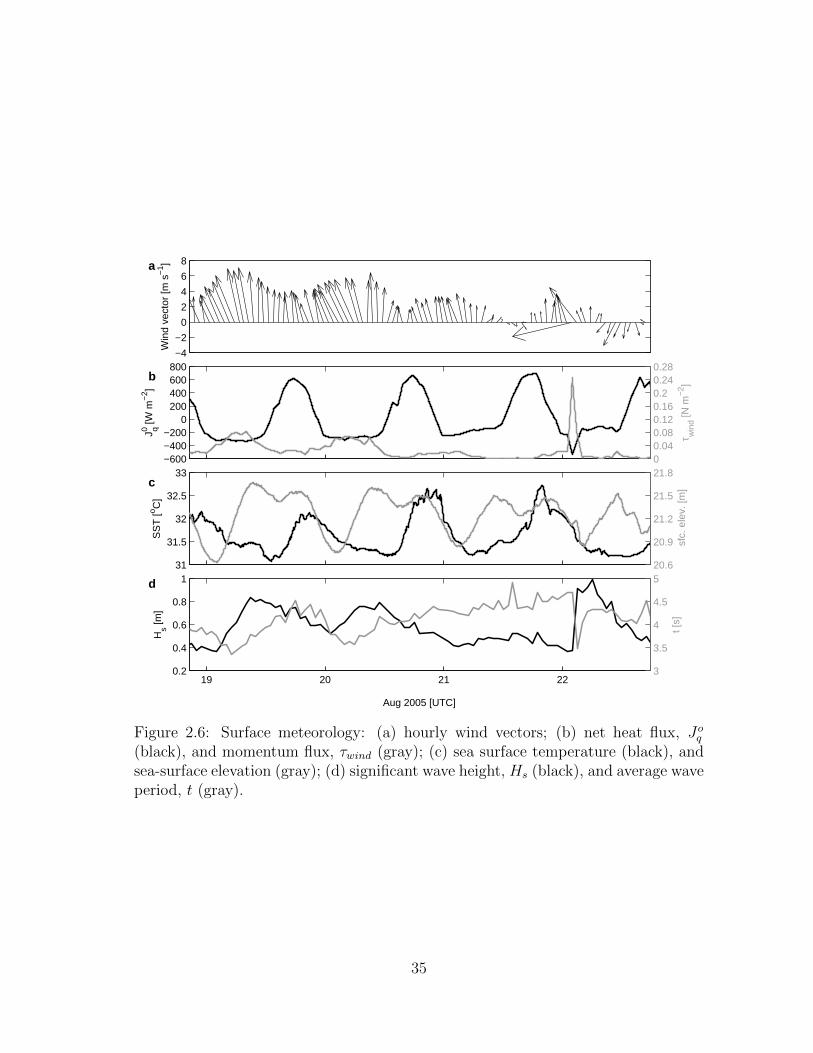
2.6 Surface meteorology: (a) hourly wind vectors; (b) net heat flux, Joq(black), and momentum flux, τwind (gray); (c) sea surface temperature(black), and sea-surface elevation (gray); (d) significant wave height,Hs (black), and average wave period, t (gray). . . . . . . . . . . . . . 35

2.7 (a) ε estimated from observations and equation (2.2); (b) ADV mea-sured current speed; (c) u (black), and v (gray); (d) ratio of σ toburst-averaged current speeds, βV , in the BBL. . . . . . . . . . . . . 38

2.8 Scatter plot of ε values calculated from vertical velocities following theTrowbridge and Elgar (2001) method (equation 2.2) and the originalmethod (equation 2.1). The slope of the linear fit is 0.44. . . . . . . . 39

2.9 Hydrographic observations: (a) potential temperature, θ; (b) salinity,S; (c) σθ; (d) squared buoyancy frequency, N2; (e) u and (f) v profilesmeasured by the ADCP; (g) squared shear frequency, M2; (h) gradientRichardson number, Ri. . . . . . . . . . . . . . . . . . . . . . . . . . 43

2.10 Depths of the RBR CTD. Due to calm conditions from late Aug. 22at site D, the WireWalker suspended at certain depths. . . . . . . . . 44

2.11 Temperature measurements from the ADCP, bottom HOBO, and ADVon the pod. . . . . . . . . . . . . . . . . . . . . . . . . . . . . . . . . 45

xv

2.12 θ-S diagram of CTD measurements at the lower end of each profile.The linear fit (solid line) has a slope -0.43. . . . . . . . . . . . . . . . 45

2.13 Velocity measurements from the ADV and the lowest two cells ofADCP. For clarity, the ADCP measurements were offset by 0.36 and0.76 m s−1 for cells 1 and 2, respectively. . . . . . . . . . . . . . . . . 47

2.14 The geometry of ADCP sidelobe interference. RMAX = Hcosα is themaximum range of good data, α = 25 is the angle from the beam tovertical direction, hence RMAX = 0.9H. The sidelobe acoustic energyreflected by the surface contaminates the near-surface measurements.The green check marks indicate good cells, while measurements inthe cells of red cross marks off RMAX is rejected (Aquadopp CurrentProfiler User Guide, Nortek). . . . . . . . . . . . . . . . . . . . . . . 48

2.15 Comparisons of turbulence quantities computed from observations tothose from the CH and SG models in the BBL: (a) ε, (b) TKE, (c) τ ,and (d) Ri (Rc

i = 1 is indicated by a horizontal dash-dot line). . . . . 52

2.16 Scatter plots (log scales) for the observations (abscissas) and the CHand SG models (ordinates) for ε (a, b), TKE (c, d), and τ (e, f).Linear fits were calculated using the RR and are represented by thesolid lines. . . . . . . . . . . . . . . . . . . . . . . . . . . . . . . . . . 55

2.17 Ratios of SG model values to CH model values for (a) TKE obtainedfrom transport equations (2.14) and (2.16), (b) ε, (c) τ , and (d) Ri. . 56

2.18 Ratios of SG model values to CH model values for (a) Γq/Γk, (b) P ,(c) B, (d) νt, (e) ν ′t, (f) M2, and (g) N2. . . . . . . . . . . . . . . . . 58

2.19 Ratios of τ values between the models: (a) SG/CHx; (b) SGx/CH;(c) SG/SGx; (d) CHx/CH. . . . . . . . . . . . . . . . . . . . . . . . . 59

3.1 The measurements were conducted at site C on the Texas - Louisianacontinental shelf. Net longwave radiation from NCEP was interpo-lated to site C; downward shortwave radiation was observed at firestation McFaddin; LUML1 buoy station that provided the rest of me-teorological data required for calculations of surface heat and momen-tum fluxes. Velocity measurements were rotated to along-shelf (u) andcross-shelf (v) directions as presented by the axis system on the fig-ure. Site D, about 150 km west of site C, included a bottom-mountedupward looking acoustic Doppler current profiler (ADCP). . . . . . . 68

3.2 Meteorological measurements: (a) hourly wind vector; (b) sea surfacetemperature; (c) heat flux, Joq (black), and momentum flux, τwind (gray). 69

xvi

3.3 (a) surface elevation; SCAMP profiles of (b) θ, (c) S, and (d) σθ. TheSBLs and BBLs defined in θ (b), S (c), and σθ (d) profiles are markedby black dots where the values are 0.1 units different than those atthe surface and at the bottom, respectively. Profiles are offset by 0.3units and aligned with the time in (a). Time intervals between profilesare ∼ 7 min. . . . . . . . . . . . . . . . . . . . . . . . . . . . . . . . . 71

3.4 Contours from SCAMP profiles at site C: (a) potential temperature,θ; (b) salinity, S; (c) σθ; (d) buoyancy frequency squared, N2. TheSBLs and BBLs defined in θ (a), S (b), and σθ (c, d) are marked bywhite dots. . . . . . . . . . . . . . . . . . . . . . . . . . . . . . . . . . 72

3.5 Ship hull-mounted ADCP velocity contours between depths 12.4 and18.4 m at site C: (a) along-shelf velocity, u; (b) cross-shelf velocity, v;(c) current speed; (d) current direction (0 is the along-shelf directionand angles increase counter-clockwise). The BBL defined in σθ ismarked by white dots. . . . . . . . . . . . . . . . . . . . . . . . . . . 73

3.6 Current measurements: along-shelf velocities at site C (a) and D (b);cross-shelf velocities at site C (c) and D (d). A white line at 12.4 mwas added on panels b and d to indicate the start depth of currentmeasurements at site C. Currents at site D were measured from anupward looking ADCP (Nortek 1 MHz Aquadopp). . . . . . . . . . . 74

3.7 Measurements from the CTD on the research vessel: (a) dissolvedoxygen; (b) hourly averaged current vectors at 15 m. . . . . . . . . . 75

3.8 (a) an example of a high turbulence energy profile taken at 3:22:00,showing potential temperature, θ (black), and vertical gradient of po-tential temperature, ∂zθ (gray); (b) observed spectra (solid line) andfit (dashed line) of a theoretical Batchelor spectrum for the profilesegment (7.9 - 8.4 m) marked by two dashed horizontal lines in (a).SCAMP’s noise level is shown by the dotted line; (c) similar to (a)but for a relatively low turbulence energy profile taken at 11:08:38.Note the scale for ∂θ/∂z is smaller than that in (a) by a factor of 4;(d) observed spectra and fit for the profile segment between 18.8 and19.4 m marked by two dashed horizontal lines in (c). . . . . . . . . . 78

3.9 Turbulent oxygen flux, O′2w′, throughout the water column. Positive

(negative) values indicate upward (downward) fluxes. . . . . . . . . . 79

3.10 (a) vertically averaged dissolved oxygen in the water within the twolayers of DO = 2 ml l−1 between depths of 6 and 15 m; (b) sum of theturbulent oxygen fluxes at the layers. . . . . . . . . . . . . . . . . . . 80

xvii

3.11 (a) observed χ; (b) CH modeled χ; (c) SG modeled χ; (d) observed ε;(e) CH modeled ε; (f) SG modeled ε. The SBL and BBL defined inσθ are marked by white dots. . . . . . . . . . . . . . . . . . . . . . . . 83

3.12 (a) observed N2; (b) CH modeled N2; (c) SG modeled N2; (d) ob-served M2; (e) CH modeled M2; (f) SG modeled M2. The SBL andBBL defined in σθ are marked by white dots. . . . . . . . . . . . . . . 84

3.13 (a) observed Ri; (b) CH modeled Ri; (c) SG modeled Ri; (d) verticallyaveraged observed χ and ε in the BBL; (e) vertically averaged Ri ofobservations and CH and SG model simulations in the BBL. The BBLdefined in σθ is marked by white dots. . . . . . . . . . . . . . . . . . 85

3.14 Observed and CH and SG modeled χ and ε profiles temporally aver-aged in (a,e) 22:00 - 23:00, (b,f) 2:00 - 3:00, (c,g) 14:00-15:00, and theentire time (d,h), respectively. Ensemble averaged SBLs and BBLsare marked by horizontal solid lines. . . . . . . . . . . . . . . . . . . . 87

3.15 Ratios of SG model values to CH model values for (a) χ and (b) ε.The SBL and BBL defined in σθ are marked by white dots. . . . . . . 89

3.16 Eddy diffusivity of temperature (ν ′t) from (a) the observations, (b) theCH model, and (c) the SG model; eddy diffusivity of density (ν ′ρ) of(d) the observations, (e) the CH model, and (f) the SG model. TheSBL and BBL defined in σθ are marked by white dots. . . . . . . . . 90

3.17 Ratios of SG model values to CH model values for (a) ν ′t and (b) ν ′ρ.The SBL and BBL for σθ are marked by white dots. . . . . . . . . . . 91

A.1 The storm was revealed by the faster SST decrease from the HOBOafter Aug 22 2:26 (black) and the reverse temporal pressure gradientfrom the ADV after Aug 22 2:00 (gray). . . . . . . . . . . . . . . . . 121

C.1 Mean values of ε for the CH model in the BBL as a function of re-laxation time in the range from 10 s to 320 minutes. Exponential fitswere calculated for velocities, and θ and S, respectively. The meanvalue of observed ε is represented by the dashed line. . . . . . . . . . 124

xviii

LIST OF TABLES

TABLE Page

1.1 Types of data measured from our instruments. The CTD at site C wasship deployed, and the CTD at site D was mounted on the WireWalker.The ADCP at site C was ship-hull mounted, and the ADCP at site Dwas bottom mounted. . . . . . . . . . . . . . . . . . . . . . . . . . . . 10

2.1 Daytime and nighttime averages of momentum flux, τwind, net heatflux, J0

q , significant wave height, Hs, average wave period, t, and meanwave direction, δ (from where waves are coming clockwise from North). 41

2.2 Minima, maxima, mean values, and 95% confidence intervals for ε,TKE, τ , and Ri for the observations, and the CH and SG models.Simulated TKE values less than 1.5 times vertical noise energies werediscarded according to equation (2.5), and the corresponding pointswere removed for other modeled quantities as well. . . . . . . . . . . . 53

2.3 Cross-correlations and 95% confidence intervals between the observa-tions and the CH and SG models for ε, TKE, and τ . . . . . . . . . . 54

2.4 Minima, maxima, and mean values with 95% confidence intervals forε, TKE, τ , and Ri for the cross-combined models CHx and SGx. Sim-ulated TKE values less than 1.5 times vertical noise energies werediscarded according to equation (2.5). Corresponding points were re-moved for other modeled quantities as well. . . . . . . . . . . . . . . 55

3.1 Mean values and 95% confidence intervals (in square brackets) for χand ε computed over the period of the experiment using the bootstrapmethod with 1000 samples (Emery and Thomson, 2001). . . . . . . . 82

3.2 Cross-correlation values and 95% confidence intervals (in square brack-ets) for χ and ε computed over the period of the experiment using thebootstrap method with 1000 samples. . . . . . . . . . . . . . . . . . . 88

3.3 Mean values and 95% confidence intervals (in square brackets) for ν ′tand ν ′ρ computed over the period of the experiment using the bootstrapmethod with 1000 samples. . . . . . . . . . . . . . . . . . . . . . . . . 89

3.4 Cross-correlations and 95% confidence intervals (in square brackets)for ν ′t and ν ′ρ were computed over the period of the experiment usingthe bootstrap method with 1000 samples. . . . . . . . . . . . . . . . . 91

xix

1. INTRODUCTION

1.1 Background

Turbulence is a random process. It transfers kinetic energy from larger to smaller

scales, eventually dissipating this energy to heat through viscous processes. Turbu-

lent processes tend to homogenize the fluid, enhance mixing, and increase transport

rates of momentum, mass, and energy. These processes happen everywhere and are

crucial in controlling flow dynamics and exchanges of momentum and water proper-

ties. However, turbulence is a research area in classical physics that is not yet fully

understood. One of the reasons is due to its characteristics of chaos and randomness.

The non-linear instability of turbulent flows makes the prediction of turbulence only

possible in statistical ways.

Turbulence energy is supplied from different sources in different layers of the

water column. In general, the latter is divided into surface boundary layer (SBL),

mid layer, and bottom boundary layer (BBL).

In the SBL, turbulence energy is chiefly provided by surface forcing, e.g. momen-

tum flux (τwind) and heat flux (J0q ), and mixes tracers, e.g. temperature (T ), salinity

(S), and dissolved oxygen (DO). τwind is transferred by wind from the atmospheric

surface layer to the SBL, and is commonly calculated using bulk parameterization

of air-sea fluxes (Fairall et al., 1996, 2003):

τwind = ρaCDU2r , (1.1)

where ρa is the air density, CD is the drag coefficient, and Ur is the mean wind speed

at a reference height (typically 10 m) above the sea level (Large and Pond , 1981).

1

Figure 1.1: Net surface heat flux (J0q ) consists of net flux of solar energy into the sea

(Jswq ), net flux of infrared radiation from the sea (J lwq ), net latent heat flux due toevaporation or condensation (J lq), and net sensible heat flux due to conduction (Jsq ).Gain of heat in the ocean is considered positive, and loss is negative.

2

J0q is the net surface heat flux. It changes the density of surface waters, thus the

buoyancy. The net heat flux budget can be expressed as the sum of four individual

components (Figure 1.1):

J0q = Jswq + J lwq + J lq + Jsq , (1.2)

where Jswq is the net flux of solar energy into the sea, −J lwq is the net flux of infrared

radiation from the sea, J lq is the net latent heat flux due to evaporation or conden-

sation, and Jsq is the net sensible heat flux due to conduction. Gain of heat in the

ocean, i.e. downward heat flux, is considered positive.

In the mid layer, internal wave breaking is the major source of turbulence energy.

Internal waves are generated where stratification occurs, and although turbulence

may be damped by stable stratification, when internal waves break, vertical mixing

will take place. Another source of turbulence energy in the mid layer is the horizontal

advection of water, the inflow would lead to intensified shear stress for vertical mixing.

In the BBL, turbulence energy is provided through shear stress induced by friction

from the seabed. BBL turbulence may affect the distribution of sediments, and

transport of particles and nutrients. The BBL generally is divided into three layers,

a bed layer, a logarithmic layer and an outer layer (Figure 1.2, Kundu and Cohen,

2008). The bed layer is viscous and velocity fluctuations are minimal. The thickness

of the bed layer is a few centimeters close to the bottom, in which shear stress is

considered uniform and is equal to the stress (τ0) at the bottom. The mean velocity

(u) is linearly distributed with distance (z) to the bottom:

µdu

dz= τ0, (1.3)

3

Figure 1.2: The BBL is divided into a viscous layer, a logarithmic layer, and an outerlayer. u∞ is the free-stream mean velocity. Heights of the three layers are sketchedfor clear identification and are not drawn to scale proportionally.

4

where µ is the dynamic viscosity. The logarithmic layer is a few meters thick. It has

the general velocity profile

u

u∗=

1

κlnz + const, (1.4)

where κ ≈ 0.41 is the von Karman constant, and u∗ is the friction velocity given by:

u∗ =

√τ0ρ, (1.5)

where ρ is the water density. Equation (1.4) is called the law of the wall, and is valid

only in the relatively thin layer in which z is greater than about 50ν/u, but less than

about 0.2h (Trowbridge et al., 1989), where ν = 1 × 10−6 m2 s−1 is the kinematic

viscosity, and h is the water depth. For a hydrodynamically rough surface, it becomes

u

u∗=

1

κlnz

z0, (1.6)

where z0 is the height at which u = 0 near the bottom. The outer layer is above

the logarithmic layer with u = 0.99u∞ on top, where u∞ is the free-stream mean

velocity. The velocity distribution is given by the velocity defect law:

u− u∞u∗

= f

(z

δz

), (1.7)

where δz is the thickness of the BBL. Turbulence in the outer layer mainly depends

on wall-free currents.

1.2 Objectives

Research on turbulence may help to understand dynamics in water columns under

specific circumstances e.g., in our case, hypoxia. The Texas-Louisiana continental

shelf, where our studies are located, has one of the biggest hypoxic zones around the

5

world (Dale et al., 2010). The hypoxia is mainly caused by fresh water discharge and

nutrient input from the Mississippi and Atchafalaya rivers (Rabalais et al., 2002).

Hypoxic zones usually form in the BBL (Dagg et al., 2007), and the benthic ecosys-

tem, as a result, is harmed by the depletion of DO near the bottom. Thus, it is

critical to investigate water dynamics in the hypoxic zone so that plans for hypoxia

management could be designed (Walker et al., 2005). Here we examine the dynamics

on the shelf focusing on turbulence.

Turbulence dynamics are described through turbulent fluxes, e.g. momentum

flux (u′w′ and v′w′), heat flux (T ′w′), and salinity flux (S ′w′). However, it is difficult

to observe those turbulent fluxes directly, thus studies usually are carried out using

statistical analyses of turbulence quantities, e.g. turbulence kinetic energy (TKE),

dissipation rate of TKE (ε), dissipation rate of temperature variance (χ), Reynolds

stress (τ), eddy diffusivity of temperature (ν ′t), and eddy diffusivity of density (ν ′ρ).

On one hand, high sampling rate instruments were developed for measuring currents

(Adrian, 1991; Voulgaris and Trowbridge, 1998; Nystrom et al., 2002), temperature

and salinity (MacIntyre et al., 1999; Bourgault et al., 2008), oxygen (Berg et al.,

2003) etc.; on the other hand, numerical turbulence models have been developed

using strategies such as direct numerical simulation (DNS, Moin and Mahesh, 1998),

large eddy simulation (LES, Mason, 1994; Meneveau and Katz , 2000), and statistical

turbulence closure models (Burchard et al., 2008). It is advantageous to understand

turbulence dynamics through a combination of observations of turbulence quantities

and numerical model simulations.

The present research consists of two studies. In the first study, measured high-

resolution velocities at one point in the BBL are used for observational schemes. The

other measured parameters, e.g. profiles of velocity, temperature, and salinity, and

surface heat and momentum fluxes, are used to force numerical turbulence models.

6

Figure 1.3: Measurements for the two studies were conducted, respectively, at sitesC and D on the Texas - Louisiana continental shelf. Distance between the two sitesis 150 km. Downward shortwave radiation was obtained from the weather stationMcFaddin. Wind speed, air temperature, relative humidity, and air pressure weremeasured at NDBC stations LUML1 and 42035, and were used for calculations ofmomentum flux, and sensible and latent heat fluxes for sites C and D, respectively.Depth contours are in m.

The turbulence quantities estimated from observations and model simulations are

compared, and differences between the models are investigated. In the second study,

χ, ε, ν ′t, and ν ′ρ are estimated from high-resolution measurements of temperature

throughout the water column at a nearby site, and the same models as in the first

study are used to compare numerical simulation results to observations.

1.3 Study sites

A field campaign as part of the NOAA Mechanisms Controlling Hypoxia (MCH)

project was conducted on the continental shelf of the Gulf of Mexico in Aug., 2005

during hypoxic conditions (Rabalais et al., 2007). The MCH aimed to study hy-

poxia and its relation to physical and biogeochemical processes (for details see

7

http://hypoxia.tamu.edu). Measurements for the first study were carried out at

site D (295′45′′N 9329′44′′W, Figure 1.3) 73 km off the coast from Aug. 18 to 24,

and those for the second study were carried out at site C (2856′55′′N 9157′5′′W,

Figure 1.3) 58 km off the coast from Aug. 22 20:00 to Aug. 23 20:00. Both sites

have water depths ∼ 21 m. Time is given in UTC (CDT + 5 h).

1.4 Instrumentation

General types of instruments for turbulence measurements are introduced in Sec-

tion 1.4.1, and the instruments used in our studies and the parameters they measure

are presented in Section 1.4.2.

1.4.1 General types of instruments for turbulence measurements

The first measurements of oceanic turbulence were made by Grant et al. (1962)

using a hot film anemometer in a tidal channel. From then on, many measuring

devices were designed and implemented (Lueck et al., 2002; Burchard et al., 2008).

Hot-film anemometers and cold-film thermometers were employed in early studies,

and were later replaced by shear probes and micro-thermistors (Lueck et al., 2002).

Shear probes use piezoceramic beams which are sensitive to the cross-stream com-

ponents of the flow, and the consequent lifting force is converted to a proportional

voltage. Lueck et al. (2002) gave a review of shear probes, and Prandke et al. (2000)

detailed the processing of probe data. Application examples of shear probes are:

Lueck and Huang (1999) deployed multiple shear probes 15 m above the sea floor at

the mid depth of a channel; Rippeth et al. (2003) measured the current microstruc-

ture from ∼ 5 m beneath the surface to 0.15 m above the seabed by a Fast Light

Yo-yo (FLY) shear probe (Dewey et al., 1987); Wolk et al. (2002) assembled a shear

probe with other sensors to a profiler called TurboMAP. The TurboMAP resolved ε

values as low as 5× 10−10 m2 s−3 in an off-shelf region.

8

Another type of instruments is designed to use the Doppler effect. The pulse is

reflected back from moving particles advected by the flow with different frequencies

of sound waves, and the speed of the particles is calculated from the change of

the reflected sound frequency due to the current (Voulgaris and Trowbridge, 1998).

Those instruments include acoustic Doppler current profilers (ADCPs) and acoustic

Doppler velocimeters (ADVs). The ADCP measures currents in vertical profiles with

different bin sizes. High-frequency ADCPs have been employed in many shelf and

estuarine studies for turbulence measurements (e.g., Stacey et al., 1999a,b; Rippeth

et al., 2002), assuming the homogeneity of statistics along beams and large-scale

anisotropy (Nystrom et al., 2007). Stacey et al. (1999a) and Rippeth et al. (2002)

calculated TKE and τ in tidal flows from ADCPs. Stacey et al. (1999b) estimated

ε and τ in a partially stratified estuary from an ADCP. Lu et al. (2000) deployed

an ADCP in a swift tidal channel with weak stratifications for τ estimation. The

ADV measures currents at high sampling rate in a small sampling water volume

(Kraus et al., 1994; Lane et al., 1998; Voulgaris and Trowbridge, 1998; Lopez and

Garcia, 2001). For a detailed evaluation of ADV for turbulence measurements, see

Voulgaris and Trowbridge (1998). Application examples of ADVs are : Voulgaris

and Trowbridge (1998) measured ε 3.1 cm above the bottom of a laboratory flume;

Richards et al. (2013) investigated the effect of shoaling internal wave on turbulence

in an estuary; Inoue et al. (2008) used an ADV attached to an elevation system to

measure vertical profiles of flow from 0.1 - 27 cm above the sediment surface.

Particle image velocimetry (PIV) systems have been used in oceanic turbulence

measurements (Liu et al., 1994; Bertuccioli et al., 1999; Doron et al., 2001; Smith

et al., 2002, 2005). The PIV illuminates the fluid with a laser sheet and takes snap-

shots of the microscopic tracer particles. The displacements of particles represent

the currents, thus 2-dimensional velocity distributions are captured. PIV has been

9

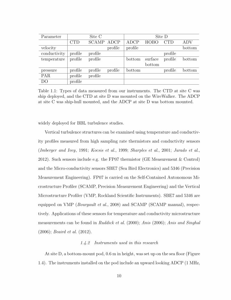
Parameter Site C Site DCTD SCAMP ADCP ADCP HOBO CTD ADV

velocity profile profile bottomconductivity profile profile profiletemperature profile profile bottom surface

bottomprofile bottom

pressure profile profile profile bottom profile bottomPAR profile profileDO profile

Table 1.1: Types of data measured from our instruments. The CTD at site C wasship deployed, and the CTD at site D was mounted on the WireWalker. The ADCPat site C was ship-hull mounted, and the ADCP at site D was bottom mounted.

widely deployed for BBL turbulence studies.

Vertical turbulence structures can be examined using temperature and conductiv-

ity profiles measured from high sampling rate thermistors and conductivity sensors

(Imberger and Ivey , 1991; Kocsis et al., 1999; Sharples et al., 2001; Jurado et al.,

2012). Such sensors include e.g. the FP07 thermistor (GE Measurement & Control)

and the Micro-conductivity sensors SBE7 (Sea Bird Electronics) and 5346 (Precision

Measurement Engineering). FP07 is carried on the Self-Contained Autonomous Mi-

crostructure Profiler (SCAMP, Precision Measurement Engineering) and the Vertical

Microstructure Profiler (VMP, Rockland Scientific Instruments). SBE7 and 5346 are

equipped on VMP (Bourgault et al., 2008) and SCAMP (SCAMP manual), respec-

tively. Applications of these sensors for temperature and conductivity microstructure

measurements can be found in Ruddick et al. (2000); Anis (2006); Anis and Singhal

(2006); Beaird et al. (2012).

1.4.2 Instruments used in this research

At site D, a bottom-mount pod, 0.6 m in height, was set up on the sea floor (Figure

1.4). The instruments installed on the pod include an upward looking ADCP (1 MHz,

10

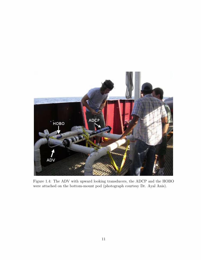
Figure 1.4: The ADV with upward looking transducers, the ADCP and the HOBOwere attached on the bottom-mount pod (photograph courtesy Dr. Ayal Anis).

11

Figure 1.5: The CTD attached at the center of the WireWalker was ready to belowered into the sea for autonomous profiling powered by surface wave energy (pho-tograph courtesy Dr. Ayal Anis).

12

Nortek Aquadopp), an ADV (1–64 Hz, Nortek Vector) and a temperature logger (up

to 1 Hz, Onset HOBO). The Conductivity, Temperature, and Depth instrument (up

to 6 Hz, RBR CTD) was mounted on a WireWalker, a surface-wave powered vehicle

(Rainville and Pinkel , 2001), and profiled along a vertical wire autonomously (Figure

1.5). Another HOBO was attached beneath the surface buoy to record sea surface

temperature (SST).

At site C, another ADCP (150 kHz, Teledyne RD Instruments) was mounted on

the hull of the research vessel Gyre. Free-falling casts of the SCAMP (profile rate

100 Hz) were conducted. The SCAMP includes two fast thermistors, a fast con-

ductivity sensor, an accurate conductivity-temperature sensor, a depth transducer,

and a photosynthetically active radiation (PAR) sensor. The CTD (24 Hz, Sea-

Bird Electronics SBE 911) on the R/V Gyre measured temperature, conductivity,

pressure, fluorescence, DO, and PAR. A summary of the instruments and measured

parameters is given in Table 1.1.

Measurements from the ADV were used for estimation of ε, TKE, and τ in the

BBL at site D, and those of the SCAMP were used for estimations of χ, ε, ν ′t, and

ν ′ρ throughout the water column at site C. Observational data (e.g. hydrographic

data and surface meteorology) were used for turbulence simulations by numerical

modeling methods.

1.5 Observational analytical methods

Next, the methods used to calculate the turbulence quantities, ε, TKE, τ , χ, ν ′t,

and ν ′ρ are introduced.

ε in isotropic turbulence can be calculated from the microstructure velocity shear

∂u∂z

or ∂u∂x

:

ε =15

2ν

(∂u

∂z

)2

= 15ν

(∂u

∂x

)2

, (1.8)

13

∂u∂z

can be converted from the measured temporal gradient ∂u∂t

using Taylor’s frozen

turbulence hypothesis (Taylor , 1938; Oakey , 1982):

∂u

∂z=

1

W

∂u

∂t, (1.9)

where W is the free-falling speed of the profiler.

ε can also be estimated using Kolmogorov’s -5/3 hypothesis (Kolmogorov , 1941)

and the energy spectrum of velocity fluctuations. In the inertial subrange, between

the energy-containing range and the dissipation range, the energy spectrum is given

by:

E(kwn) = αε23k− 5

3wn , (1.10)

where α is the Kolmogorov constant, and kwn is the radian wavenumber. This

equation describes that E(kwn) decays with a −53

slope in logarithmic scale. Since

velocities are measured in the time domain, Taylor’s frozen turbulence hypothesis can

be applied to convert the energy spectrum from frequency (f) space to wavenumber

space as follows:

E(kwn) =E(f)U

2π, (1.11)

where U is the mean horizotal current velocity. ε can then be estimated from

E(f) = (2π)−23U−

83αε

23f−

53 (1.12)

by fitting a -5/3 line to the spectrum in the inertial subrange. This method has

been applied to measurements from different types of instruments, e.g. ADV (Gross

and Nowell , 1985; McPhee, 1998), PIV (Bertuccioli et al., 1999), and ADCP (Jonas

et al., 2003).

14

TKE is a function of the variances of u, v, and w in an isotropic flow and is given

by

k =1

2

(u′2 + v′2 + w′2

). (1.13)

In general, τ is given by

τ = ρu′w′ or τ = ρv′w′, (1.14)

while in the bed layer where the flow is steady and homogeneous (Perlin et al., 2005;

Arneborg et al., 2007),

ε = −u′w′dUdz, (1.15)

where

u′w′ = u2∗, (1.16)

and

dU

dz=u∗l, (1.17)

l = κz, (1.18)

such that

ε =u3∗κz, (1.19)

and according to equation (1.5), τ can be expressed by

τ = ρ(εκz)23 . (1.20)

χ is calculated from the integral of the spectrum of the vertical gradient of tem-

15

perature fluctuations ∂zT′:

χ = 6ν ′(∂zT ′)2 = 6ν ′∫ ∞t

(Sobs(kwn)− Sn(kwn)

)dkwn, (1.21)

where ν ′ is the thermal diffusivity , kwn = kwn/2π is the cyclic wavenumber, Sobs is

the observed spectrum, and Sn is the instrument’s noise spectrum.

ε can be estimated by fitting the spectrum of ∂zT′ to the theoretical Batchelor

spectrum (Dillon and Caldwell , 1980; Oakey , 1982), and is expressed as:

ε = k4Bνν′2, (1.22)

where kB is the Batchelor cutoff wavenumber estimated from the Batchelor spectrum:

S(kwn) =(q

2

) 12 χ

kBν ′g(q, kwn/kB), (1.23)

where q is between 3.4 and 4.1 (Dillon and Caldwell , 1980; Oakey , 1982), and

g(q, kwn/kB) = 2π

(e−α

2/2 − α∫ ∞α

e−x2/2dx

), (1.24)

where

α = (2q)12

2πkwnkB

. (1.25)

ν ′t and ν ′ρ are functions of χ and ε, respectively, and are given by

ν ′t =χ

2

(∂T

∂z

)−2, (1.26)

and

ν ′ρ = Γε

N2, (1.27)

16

where Γ is the mixing efficiency, it varies between 0.04 and 0.4 (Peters et al., 1995)

and is commonly chosen as 0.2 (Osborn, 1980; Moum, 1996; Nash et al., 2007).

1.6 Turbulence numerical models

1.6.1 Types of numerical models

The development of turbulence models has a history for decades. All models are

based on the Navier-Stokes equations with the Boussinesq approximation (Boussi-

nesq , 1903; Spiegel and Veronis , 1960):

∂tvi + vj∂jvi − ν∂jjvi + 2εijlΩjvl = −∂ipρ0− giρ0ρ, (1.28)

and the continuity equation:

∂jvj = 0, (1.29)

where the subscripts i,j,l denote axes in a Cartesian coordinate system, v is the

current velocity, Ω is the rotation rate of the earth, p is the pressure, ρ0 is a constant

reference density, g is the gravitational acceleration, ρ is the potential density, and

εijl is the alternating tensor (Kundu and Cohen, 2008). The tracer equations for T

and S are required for ρ calculation, and can be derived by approaches similar to

the Navier-Stokes equations. The equation for T is

∂tT + vj∂jT − νT∂jjT =∂zI

cpρ0, (1.30)

where νT is the thermal diffusivity, I is the local solar radiation in the water, and cp

is the heat capacity of water. S is expressed by

∂tS + vj∂jS − νS∂jjS = 0, (1.31)

17

where νS is the haline diffusivity. ρ can be calculated as a function of T , S, and p

through a state equation:

ρ = ρ(T, S, p). (1.32)

The numerical solutions for hydrodynamical processes can be found from the set of

Eq. (1.28) - (1.32), and the methods include DNS (e.g. Smyth et al., 2001), LES (e.g.

Skyllingstad et al., 1999), and one-point closure models (e.g. Umlauf and Burchard ,

2005).

DNS resolves viscous scales, thus computational limits restrict its applications

to small-scale eddies with low Reynolds number Re = vL/ν up to 104. In the

oceanic mixed layer, a typical velocity scale of v = 0.1ms−1, a length scale of L = 1

m, and ν = 10−6m2s−1 for water at 20C result in Re = 105; in the open ocean,

L = 106 m, Re = 1011, thus DNS is incapable of resolving large (i.e. energy-

containing) eddies. One attempt to solve the shortcoming of DNS is LES. LES

applies to convective turbulence in which the size of eddies is relatively large with

respect to the relevant mean flow scale (e.g. the mixed layer depth) processes. LES, in

constrast, is computationally costly for resolving small size energy-containing eddies.

One-point closure models use parameterizations to simulate turbulence in a statis-

tical sense. Velocity, temperature, pressure and salinity are commonly investigated

by decomposing these variables into mean and fluctuating components (Reynolds

decomposition, Reynolds , 1895; Lesieur , 2008). For instance, the velocity is given

by:

vi = vi + v′i, (1.33)

Equations (1.28) - (1.31) are then given by:

∂tvi + vj∂jvi − ∂j(ν∂jvi − v′jv′i

)+ 2εijlΩjvl = −∂ip

ρ0− gi

ρ

ρ0, (1.34)

18

∂jvj = 0, (1.35)

∂tT + vj∂jT − ∂j(νT∂jT − v′jT ′

)=

∂zI

cpρ0, (1.36)

∂tS + vj∂jS − ∂j(νS∂jS − v′jS ′

)= 0. (1.37)

There are unknown second-moment turbulent fluxes in the equations, i.e. Reynolds

stress v′jv′i, turbulent heat flux v′jT

′, and turbulent salt flux v′jS′, which need to be

resolved by the transport equations at the next higher order:

∂tv′iv′j + ∂l

(vlv′iv

′j + v′lv

′iv′j − ν∂lv′iv′j

)= −∂lviv′lv′j − ∂lvjv′lv′i − 2Ωl

(εilmv′jv

′m + εjlmv′iv

′m

)− 1

ρ0

(giv′jρ

′ + gjv′iρ′)− 1

ρ0v′i∂jp

′ + v′j∂ip′

− 2ν∂lv′j∂lv′i,

(1.38)

∂tv′iT′ + ∂j

(vjv′iT

′ + v′iv′jT′ − (ν + ν ′)∂jv′iT

′)

+ ν ′T ′∂jjv′i + νv′i∂jjT′

= −v′iv′j∂jT − ∂jviv′jT ′ − 2εijlΩjv′lT′

− giρ0T ′ρ′ − 1

ρ0T ′∂ip′ + v′j∂ip

′ − 2(ν + ν ′)∂jv′i∂jT′,

(1.39)

∂tT ′2 + ∂j

(vjT ′2 + v′jT

′2 + ν ′∂jT ′2)

=

− 2v′jT′∂jT − 2ν ′(∂jT ′)2,

(1.40)

19

∂tT ′S ′ + ∂j(vjT ′S ′ + v′jT

′S ′ + (ν ′ + ν ′′)∂jT ′S ′)

=

− v′jS ′∂jT − v′jT ′∂jS − 2(ν ′ + ν ′′)∂jT ′∂jS ′

− ν ′T ′∂jjS ′ − ν ′′S ′∂jjT ′.

(1.41)

The undetermined third moments (v′iv′jk′k, v

′iv′jT′, v′iT

′2, v′iT′S ′) and pressure-strain

correlators∏

ij = 1ρ0v′i∂jp

′ + v′j∂ip′ and

∏iT = 1

ρ0T ′∂ip′ need to be resolved by trans-

port equations at the next higher order, and so on. The infinite repetition of this

procedure prevents turbulence equations from being closed, referred to as the clo-

sure problem (Haltiner and Williams , 1980; Vallis , 2006). To close the turbulence

transport equations, the third moments in Eqs. (1.38) - (1.41) may be neglected

assuming local equilibrium, and parameterizations for∏

ij and∏

iT to the known

second moments and mean flow quantities can be derived in several ways (Burchard ,

2002). For example,∏

ij and∏

iT have the following general expressions in Kantha

and Clayson (1994), Burchard and Baumert (1995), and Canuto et al. (2001):

∏ij

=c1ε

k

(v′iv′j −

2

3δijk

)+ c2

(Pij −

2

3δijP

)+

c3

(Bij −

2

3δijB

)+ c4

(Dij −

2

3δijP

)+

c5kSij,

(1.42)

where δij is the Kronecker symbol, Pij is the shear production:

Pij = −∂lviv′lv′j − ∂lvjv′lv′i, (1.43)

20

Bij is the buoyancy production:

Bij = − 1

ρ0

(giv′jρ

′ + gjv′iρ), (1.44)

Sij is the mean shear:

Sij =1

2(∂ivj + ∂jvi) , (1.45)

Dij is the anisotropic shear production:

Dij = −v′iv′l∂jvl − v′jv′l∂ivl, (1.46)

P is the shear production:

P = −∂ivjv′iv′j, (1.47)

and B is the buoyancy production:

B = − g

ρ0v′3ρ′; (1.48)

∏iT

=c1Tε

kv′iT

′ + c2Tv′jT′∂jui−

c3Tgiρ0∂TρT ′2 − c4Tv′iT ′Vij,

(1.49)

where Vij is the mean vorticity:

Vij =1

2(∂jvi − ∂ivj) . (1.50)

Assumptions for turbulence closures are (Burchard , 2002):

• boundary layer approximation

• neglect or simplification of second-moment transports

21

• neglect of rotational terms in the second-moment equations

• neglect of tracer cross-correlations

• parameterization of pressure-strain correlators

• parameterization of dissipation terms

The models applied in the present study are one-point statistical closure models,

which meet the requirements below (Umlauf and Burchard , 2005):

• comprehensive physical meaning

• computational economy

• numerical robustness

• applicability in three-dimensional models

Predicted turbulence quantities, e.g. TKE, ε, τ , and χ, from one-point statistical

closure models can be compared to those estimated from measurements. A large

number of comparative studies for these quantities have been reported in the liter-

ature (e.g. Clayson and Kantha, 1999; Burchard et al., 2002; Simpson et al., 2002;

Stips et al., 2002; Anis and Singhal , 2006).

Second-moment two-equation turbulence models, as one type of one-point statis-

tical closure models, have proven to be a good compromise between complexity and

simplification (Stips et al., 2002). Those models close equations (1.34) - (1.37) at

second moments, and use two transport equations for the second-moment turbulent

fluxes. One transport equation is of TKE (denoted as k in models) and the other is

of L or a L related quantity (e.g. ε, ω, or τ , Umlauf and Burchard , 2003).

The turbulent fluxes are functions of a turbulent diffusivity and a mean flow

gradient:

22

u′w′ = −νt∂u

∂z, (1.51)

v′w′ = −νt∂v

∂z, (1.52)

T ′w′ = −ν ′t∂T

∂z, (1.53)

S ′w′ = −ν ′t∂S

∂z, (1.54)

where νt is the eddy viscosity. In the k − ε turbulence closure,

νt = (c0µ)3cµk2

ε, (1.55)

ν ′t = (c0µ)3c′µk2

ε, (1.56)

and in the k − kL turbulence closure,

νt = cµk12L, (1.57)

ν ′t = c′µk12L, (1.58)

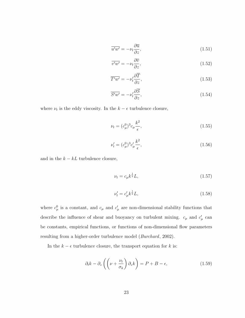
where c0µ is a constant, and cµ and c′µ are non-dimensional stability functions that

describe the influence of shear and buoyancy on turbulent mixing. cµ and c′µ can

be constants, empirical functions, or functions of non-dimensional flow parameters

resulting from a higher-order turbulence model (Burchard , 2002).

In the k − ε turbulence closure, the transport equation for k is:

∂tk − ∂z((

ν +νtσk

)∂zk

)= P +B − ε, (1.59)

23

where σk is the turbulent Schmidt number for vertical flux of TKE; the other trans-

port equation for the L related quantity is:

∂tε− ∂z((

ν +νtσε

)∂zε

)=ε

k(c1εP + c3εB − c2εε) , (1.60)

where σε is the turbulent Schmidt number for vertical flux of ε, c1ε = 1.44, c2ε = 1.92,

and c3ε = 1.

In the k − kL turbulence closure, the transport equation for k is:

∂tk − ∂z(Sq√

2kL∂zk)

= P +B − ε, (1.61)

where Sq = 0.2 (Simpson et al., 1996); the other transport equation for L related

quantity is:

∂t(kL)− ∂z(Sl√

2kL∂z(kL))

=L

2

(E1P + E3B −

(1 + E2

(L

Lz

)2)ε

), (1.62)

where Sl ≈ 0.2, E1 = 1.8, E2 = 1.33, and E3 is a function of the gradient Richardson

number (Ri) and stability functions (Mellor and Yamada, 1982).

1.6.2 The general ocean turbulence model

The one-dimensional General Ocean Turbulence Model (GOTM; Burchard 2002)

is used for the numerical simulations in the present study. The GOTM is a program

that implements different turbulence models, e.g. empirical models, two-equation

models, algebraic stress models, K-profile parameterizations (KPP), etc. The GOTM

is widely used due to less complexity and prominent contribution in saving compu-

tational time compared to three-dimensional models. Applications of the GOTM

are made for model-observation comparisons for ε (Bolding et al., 2002), χ (Anis

24

and Singhal , 2006), and depth of mixed layer (He and Chen, 2011), as well as inter-

model comparisons (Burchard and Bolding , 2001; Burchard et al., 2002). Several

processes (e.g. horizontal variability, shear instability, and internal waves) treated

prognostically in three-dimensional models have to be either prescribed or neglected,

depending on their relevance for the processes under investigation (Burchard et al.,

1999; Simpson et al., 2002; Baumert et al., 2005). Observational data can be used

as external forcing and validation. Setting of relaxation time allows for nudging

simulated hydrographic variables, e.g. temperature, salinity and current velocity, to

observed profiles, by which the horizontal gradients are provided for one-dimensional

models in the GOTM. Among the diverse second-moment two-equation turbulence

closure models, the k − kL turbulence closure models (Mellor and Yamada, 1982;

Burchard et al., 1999) and the k − ε turbulence closure models (Launder and Spald-

ing , 1972; Rodi , 1987; Burchard et al., 1998; Canuto et al., 2001) are commonly used,

and are applied in the following studies.

25

2. OBSERVATIONS AND MODEL SIMULATIONS OF TURBULENCE IN

THE BOTTOM BOUNDARY LAYER OF THE TEXAS-LOUISIANA

CONTINENTAL SHELF

2.1 Introduction

The northern Gulf of Mexico has one of the largest hypoxic regions in the world

(16,500 km2 on average; Dale et al., 2010). The formation of hypoxia is believed to

be caused primarily by excess anthropogenic nitrogen inputs to the coastal sea and

seasonal vertical stratification (Bianchi et al., 2010; Liu et al., 2010). Nitrogen inputs

elevate primary production in the surface boundary layer (SBL), and the increased

organic matter sinks to the bottom boundary layer (BBL), causing high respiration

rate. Stratification is induced by fresh water discharge and surface heating, and

suppresses vertical transport of dissolved oxygen from the surface to the bottom

through the pycnocline. These two effects result in a hypoxic bottom-water zone

(Dagg et al., 2007). Thus it is important to understand the physical processes in the

BBL where turbulence is a key parameter in the micro-scale dynamics.

Turbulence is a major driving mechanism of mixing processes and fluxes of vari-

ous waterborne substances ranging from dissolved matter to sediments. In the BBL

turbulence activity is enhanced by shear stress near the bed, and contributes to de-

struction of stratification and an increase in the vertical transport of oxygen and

nutrients. Since direct measurements of turbulence fluxes in the ocean pose signif-

icant technical difficulties, studies typically examine turbulence quantities such as

turbulence kinetic energy (TKE, denoted as k in numerical models), TKE dissipa-

tion rate (ε), and Reynolds stress (τ), from which fluxes may then be estimated

(Tennekes and Lumley , 1972).

26

Methods to study such turbulence quantities may include observations and model

simulations. Here, high-frequency measurements of current velocities from an acous-

tic Doppler velocimeter (ADV) in the BBL were used to estimate ε, using Kol-

mogorov’s -5/3 hypothesis for energy spectra in the inertial subrange (Kolmogorov ,

1941). In a shallow water environment, orbital motions due to surface waves may

affect turbulence in the BBL (Lumley and Terray , 1983; Grant and Madsen, 1986).

To remove the effects of surface-wave-induced orbital velocities (σ) in the BBL, we

applied a modified equation of energy spectrum in the inertial subrange introduced

by Trowbridge and Elgar (2001). TKE was estimated from the integration of the en-

ergy spectrum under the -5/3 logarithmic fitting line extended from the demarcation

of energy-containing range and inertial subrange (Pope, 2000) to a high frequency

end above the noise level. τ was calculated from ε according to the law of the wall

(Lee, 2003; Thorpe, 2005).

Numerical model simulations were carried out to evaluate their performance in

reproducing ε, TKE, and τ . Turbulence models have been developed and imple-

mented to simulate physical dynamics in the BBL, and a recent review by Burchard

et al. (2008) summarises details of models used to quantify turbulence in coastal

oceans. Among these models, second-moment two-equation statistical turbulence

closure models are most widely used, and are integrated in the general ocean tur-

bulence model (GOTM; Burchard et al., 1999; Burchard , 2002) used in the present

study. Models applied in our study consist of two turbulence closures, k − ε and

k − kL (L is the macro length scale), and the stability functions of Cheng et al.

(2002) and Schumann and Gerz (1995). The turbulence closures k − ε and k − kL

have been extensively applied and found to be successful in simulating turbulence

in aquatic surface and bottom boundary layers (e.g., Burchard and Bolding , 2001;

Warner et al., 2005; Anis and Singhal , 2006). The stability functions of Schumann

27

and Gerz (1995) are empirical, and those of Cheng et al. (2002) are parameterized

for second order models. Cheng et al. (2002) improved the Mellor-Yamada model

(Mellor and Yamada, 1974, 1982) using more complete expressions for pressure-

velocity and pressure-temperature correlations. Both sets of stability functions have

been successfully applied for reproducing observations (e.g. Burchard et al., 2002;

Simpson et al., 2002; Burchard et al., 2009; Hofmeister et al., 2009; Verspecht et al.,

2009). The two types of stability functions were integrated with the k− ε and k−kL

closures, and their effects on the simulation results were compared.

The study site and instruments are described in Section 2.2. A quality control

test is applied to current data from a bottom mounted ADV, and turbulence quanti-

ties (ε, TKE, and τ) are then calculated from the data (Section 2.3). Meteorological

and hydrographic data used to force turbulence models are described in Sections

2.4.1 and 2.4.2, respectively. Four models are implemented for turbulence simula-

tions and their fundamental equations are introduced in Section 2.4.3. Two of the

models, one combining the k − ε turbulence closure and the stability functions of

Cheng et al. (2002), and the other combining the k− kL turbulence closure and the

stability functions of Schumann and Gerz (1995), are compared to estimates of ε,

TKE, τ , and gradient Richardson number (Ri) from observations in the BBL. This

is followed by statistics of the other two models with reversed combinations of tur-

bulence closures and stability functions (Section 2.5.1). Inter-model comparisons for

the four models are examined throughout the water column (Section 2.5.2), and the

influence of surface fluxes on turbulence simulations in the BBL is investigated for

these models (Section 2.5.3). Differences between the turbulence closures and the

stability functions due to their physical assumptions are discussed in Section 2.6,

and conclusions are given in Section 2.7.

28

Figure 2.1: Measurements were conducted at site D on the Texas-Louisiana conti-nental shelf. Downward shortwave radiation was observed at the weather stationMcFaddin. NDBC station 42035 measured wind speed, air temperature, relative hu-midity and air pressure, which were used for calculations of surface momentum flux,and sensible and latent fluxes. Horizontal velocities were rotated to across (u) andalong (v) the principal axis of currents. Depth contours are in m.

2.2 Study site and instrumentation

A field campaign was conducted as part of the NOAA Mechanisms Controlling

Hypoxia (MCH) project from August 18 to 22, 2005 (for details see http://hypoxia.

tamu.edu). Time is given in UTC (CDT + 5 h) in this study. A multi-instrumented

pod was deployed on the sea floor at site D at a depth of 21.7 m (295′45′′N

9329′44′′W, Figure 2.1). Instruments included an upward-looking Nortek 1 MHz

Aquadopp acoustic Doppler current profiler (ADCP), a Nortek Vector ADV and an

Onset R© U22-001 water temperature logger (HOBO, response time 5 minutes, sam-

pling every 30 s, Figure 2.2b). The ADCP was set to sample current profiles every

6 minutes with vertical cell size of 0.4 m starting at 1.24 m above the bottom. The

ADV measured three-dimensional velocities 0.93 m above the bottom in burst mode,

29

Figure 2.2: (a) a CTD was attached to the WireWalker, and a HOBO temperaturelogger was attached to the mooring wire beneath the surface buoy; (b) a bottommount was instrumented with an ADV, an ADCP, and a HOBO temperature logger.

with 2048 samples per burst taken every 180 s at a sampling rate of 32 Hz (thus, the

duration of each burst was 64 s). Velocity measurements were orientated to along (v)

and across (u) the principal axis of ADV measured currents (Figure 2.3; Emery and

Thomson, 2001) that was 4 counter-clockwise from North(Figure 2.1). Tempera-

ture measurements from the bottom HOBO were compared to those from the ADV’s

thermistor (response time 10 minutes, sampling rate 1 Hz), and were found to be in

good agreement. Temperature and salinity profiles were measured by a RBR XR-620

conductivity, temperature, and depth instrument (CTD) at 1 Hz. The CTD sensor

was mounted at the center of a surface-wave powered profiling vehicle (WireWalker;

Figure 2.2a; Rainville and Pinkel 2001).

30

−0.1 −0.05 0 0.05 0.1 0.15

−0.1

−0.05

0

0.05

0.1

0.15

East speed [m s−1]

Nor

th s

peed

[m s

−1 ]

Figure 2.3: Scatter plot of ADV mean velocities. The linear fit was 4 from theNorth.

31

100

101

102

103

10−10

10−9

10−8

10−7

10−6

10−5

Wavenumber [rad m−1]

Ene

rgy

spec

trum

[(m

2 s−

2 ) / (

rad

m−

1 )]

10−1

100

101

10−8

10−7

10−6

10−5

10−4

10−3

Frequency [Hz]

Ene

rgy

spec

trum

[(m

2 s−

2 ) / H

z]

u

v

w

Figure 2.4: Energy spectra of an ADV burst measurement (2048 samples) of u (dot-ted), v (black), and w (gray) velocity components as a function of wavenumber (leftand bottom axes) and frequency (right and top axes). A -5/3 slope (dashed) is drawnin the inertial subrange for reference. The mean horizontal current speed was 0.07m s−1 and the measurements were taken on Aug. 21 9:18.

32

Figure 2.5: The ADV velocity is measured in the direction (15 from the trans-mitting beam) of the angular bisector between transmitting and receiving beams.The vertical component of velocity is closer to the transmitter than the horizontalcomponents, so that the vertical velocity has less uncertainty (Vector Current MeterUser Manual, Nortek).

33

2.3 Observational approach

High sampling rate velocity measurements from the ADV were used for estima-

tion of turbulence quantities. ε was calculated from the vertical current velocity

fluctuations, w′, after applying the Reynolds decomposition (Tennekes and Lum-

ley , 1972; Kundu and Cohen, 2008). Quality control of the ADV measurements

was performed as follows: bursts were rejected if beam velocity correlations ≤ 70%

(Vector Current Meter User Manual, Nortek); burst-averaged vertical velocities were

required to be < 0.01m s−1 such that w was close to the true vertical direction (Davis

and Monismith, 2011). Estimates of observed ε were based on Kolmogorov’s -5/3

law (Kolmogorov , 1941) and a fit to the energy spectrum of velocity fluctuations

in the inertial subrange (Jonas et al., 2003; Lorke and Wuest , 2005). In the iner-

tial subrange, the energy spectrum is expected to be a function only of ε and the

wavenumber, kwn (or frequency f), and follow a -5/3 slope in logarithmic scale:

E(kwn) = αε23k− 5

3wn , (2.1)

where E(kwn) is the energy spectrum, and α = 1.5 is the Kolmogorov constant

(Sreenivasan, 1995; Pope, 2000). An example of an energy spectrum with mean hor-

izontal current speed 0.07 m s−1 is shown in Figure 2.4. White spectral noise is visible

at the high kwn (or f) end. Noise of the vertical component (5.23×10−8m2 s−2 Hz−1

on average) is lower than that of the horizontal components (1.44×10−6m2 s−2 Hz−1

on average). The lower noise in the vertical component is due to the geometry of

the ADV transducers (Figure 2.5), with the transmitting and receiving beam pair

being more sensitive to velocities in the direction of the angular bisector between the

beams. Thus, with the transmitter configured in the vertical direction, the vertical

velocities have a lower noise level and were used for the present work.

34

−4

−2

0

2

4

6

8

Win

d ve

ctor

[m s

−1 ]

−600−400−200

0200400600800

J q0 [W m

−2 ]

00.040.080.120.160.20.240.28

τ win

d [N m

−2 ]

31

31.5

32

32.5

33

SS

T [o C

]

20.6

20.9

21.2

21.5

21.8

sfc.

ele

v. [m

]19 20 21 22

0.2

0.4

0.6

0.8

1

Hs [m

]

Aug 2005 [UTC]

3

3.5

4

4.5

5

t [s]

a

b

c

d

Figure 2.6: Surface meteorology: (a) hourly wind vectors; (b) net heat flux, Joq(black), and momentum flux, τwind (gray); (c) sea surface temperature (black), andsea-surface elevation (gray); (d) significant wave height, Hs (black), and average waveperiod, t (gray).

35

In shallow coastal waters, surface waves may create σ in the near bed region, the

depth (z) in which effects of surface waves will be important is z ≤ 0.16gt2 (Baumert

et al., 2005), where t is the wave period, and g is the gravitational acceleration. Thus,

surface waves with t > 3.6 s may have an effect in the BBL at site D (water depth of 21

m). t was primarily longer than 3.6 s at site D (for details see Section 2.4.1 and Figure

2.6d), thus, the BBL at site D was affected by surface waves (Davis and Monismith,

2011), and a removal of turbulence induced by σ was carried out. The surface wave

energy can be noted between 0.1 and 0.3 Hz in the energy spectra (Figure 2.4), also

most likely elevated the spectra in the inertial subrange. To apply the Kolmogorov’s

hypothesis to the energy produced by turbulence but not by surface wave, ε was

estimated from the equation for vertical velocity components in Trowbridge and Elgar

(2001):

Eww(f) =12

55αε

23V

23f−

53 I(

σ

V, φ) (2.2)

where Eww(f) is the energy spectrum of vertical velocity fluctuations, V is the hori-

zontal mean current, and I is the function of σ, the angle between wave and current

(φ), and V (for the expression of I see Trowbridge and Elgar 2001).

Kolmogorov (1941) hypothesized that an inertial subrange in the energy spectrum

exists only when energy is transferred by inertial forces while viscous forces are

negligible. The existence of an inertial subrange was first examined for each burst.

For instance, the energy spectra of vertical velocity fluctuations (Figure 2.4) showed

an intermediate range with a slope close to -5/3. The f range was chosen from

0.3 Hz (to exclude wave domains) to a f before noise became dominant (the range

represented by the dashed line). A robust regression algorithm (RR; Chatterjee

and Hadi , 1986; DuMouchel and O’Brien, 1991; Wager et al., 2005) was applied to

36

compute the slope and the 95% confidence interval. The RR minimizes the sum

s =N∑i=1

Wi(yi − yi)2, (2.3)

where yi is the ordinate of the observed data point, yi is the ordinate of the corre-

sponding point on the fitting line, and Wi is the weight calculated by a bi-square

weighting function, assigning less weight to outliers. If -5/3 falls within the 95% con-

fidence interval of the fitted line’s slope (here [-1.73 -1.63]), an inertial subrange was

considered to exist, and ε was estimated by applying equation (2.2). 768 out of 2356

bursts (32.6%) were found to exhibit acceptable inertial subranges, with estimated

values of ε above 5× 10−9 m2s−3.

Observed ε values (Figure 2.7a) were significantly affected by the current speeds

in the BBL and followed their pattern consistently (Figure 2.7b). Magnitudes of the

currents were mainly a function of v, given that this velocity component (0.04 m s−1

on average) generally was larger than the u component (0.02 m s−1 on average,

Figure 2.7c). Ratios of σ to burst-averaged current speed, βV , were mostly <0.5

(Figure 2.7d), indicating that surface waves had an impact near the seabed but not as

significant as reported in other shallower water experiments (Davis and Monismith,

2011; Hackett et al., 2011). To quantitatively investigate the effect of surface waves,

ε was also estimated from equation (2.1). The regression coefficient of ε values

calculated from equations (2.2) and (2.1) was 0.44 (Figure 2.8).

TKE is defined as

k =1

2

(u′2 + v′2 + w′2

), (2.4)

where overbars denote time averages. Turbulence was assumed locally isotropic, thus

37

10−8

10−7

10−6

ε [m

2 s−

3 ]

0

0.05

0.1

0.15

spee

d [m

s−

1 ]

−0.15−0.1

−0.050

0.050.1

0.15

u [m

s−

1 ]

−0.15−0.1−0.0500.050.10.15

v [m

s−

1 ]19 20 21 22

0

0.5

1

β V

Aug 2005 [UTC]

a

b

c

d

Figure 2.7: (a) ε estimated from observations and equation (2.2); (b) ADV measuredcurrent speed; (c) u (black), and v (gray); (d) ratio of σ to burst-averaged currentspeeds, βV , in the BBL.

38

0 1 2 3 4 5 6

x 10−6

0

0.5

1

1.5

2

2.5x 10

−6

εoriginal

ε Tro

wbr

idge

Figure 2.8: Scatter plot of ε values calculated from vertical velocities following theTrowbridge and Elgar (2001) method (equation 2.2) and the original method (equa-tion 2.1). The slope of the linear fit is 0.44.

39

u′2 and v′2 were replaced by w′2:

k =3

2w′2. (2.5)

w′2 was the spectral integral in the inertial subrange above the noise level. The low

end of the frequency range was chosen as 1/kwn = l0/10 (l0 = 0.93 m is the height

of the ADV’s sampling volume above the bottom), demarcating between anisotropic

large eddies and isotropic small eddies (Pope, 2000; Bluteau et al., 2011). The high

end of the frequency range was chosen where the spectrum decreased to the instru-

ment’s noise level.

Reynolds stress was estimated from the law of the wall which assumes uniform

stress near the seabed (Perlin, 2005; Arneborg et al., 2007):

τ = ρ(εκl0)23 , (2.6)

where κ = 0.41 is the von Karman constant. Results of estimated ε, TKE and τ

from the observations are further discussed in Section 2.5.

2.4 Numerical modeling approach

Models were forced with meteorological and hydrographic measurements. We

describe the surface meteorology and hydrography first, and then the formulation of

models is explained.

2.4.1 Surface meteorology

Meteorological data were obtained from the stations shown in Figure 2.1. Wind

conditions were recorded at the National Data Buoy Center (NDBC) station 42035

(2913′54′′ N 9424′46′′ W). South winds prevailed during most of the experiment,

diminishing during nighttime and increasing during daytime (Figure 2.6a). A single

strong wind event was recorded at NDBC 42035 around 04:00 on Aug. 22, with wind

40

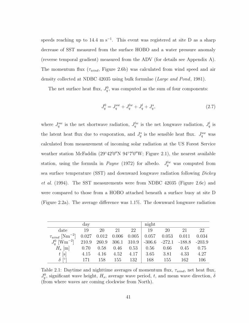
speeds reaching up to 14.4 m s−1. This event was registered at site D as a sharp

decrease of SST measured from the surface HOBO and a water pressure anomaly

(reverse temporal gradient) measured from the ADV (for details see Appendix A).

The momentum flux (τwind, Figure 2.6b) was calculated from wind speed and air

density collected at NDBC 42035 using bulk formulae (Large and Pond , 1981).

The net surface heat flux, J0q , was computed as the sum of four components:

J0q = Jswq + J lwq + J lq + Jsq , (2.7)

where Jswq is the net shortwave radiation, J lwq is the net longwave radiation, J lq is

the latent heat flux due to evaporation, and Jsq is the sensible heat flux. Jswq was

calculated from measurement of incoming solar radiation at the US Forest Service

weather station McFaddin (2942′0′′N 947′0′′W; Figure 2.1), the nearest available

station, using the formula in Payne (1972) for albedo. J lwq was computed from

sea surface temperature (SST) and downward longwave radiation following Dickey

et al. (1994). The SST measurements were from NDBC 42035 (Figure 2.6c) and

were compared to those from a HOBO attached beneath a surface buoy at site D

(Figure 2.2a). The average difference was 1.1%. The downward longwave radiation

day nightdate 19 20 21 22 19 20 21 22

τwind [Nm−2] 0.027 0.012 0.006 0.005 0.057 0.053 0.011 0.034J0q [Wm−2] 210.9 260.9 306.1 310.9 -306.6 -272.1 -188.8 -203.9Hs [m] 0.70 0.58 0.46 0.53 0.56 0.66 0.45 0.75t [s] 4.15 4.16 4.52 4.17 3.65 3.81 4.33 4.27δ [] 171 158 155 132 168 155 162 106

Table 2.1: Daytime and nighttime averages of momentum flux, τwind, net heat flux,J0q , significant wave height, Hs, average wave period, t, and mean wave direction, δ

(from where waves are coming clockwise from North).

41

was retrieved from the National Centers for Environmental Prediction/Department of

Energy Reanalysis 2 (NCEP; Sun et al., 2003; Kubota et al., 2008) database, and was

interpolated to site D using the nearest grid points. J lq and Jsq were calculated using

wind speed, air temperature, relative humidity, and air pressure from the NDBC

42035 and the SST (Fairall et al., 1996). J0q followed a diurnal pattern (Figure 2.6b),

and daytime and nighttime averages of τwind and J0q are given in Table 2.1.

The sea-surface elevation (Figure 2.6c) indicates a dominant semi-diurnal tide

with a range of up to 1 m during the study period. Significant wave height (Hs), t,

and mean wave direction (δ) were retrieved from NDBC 42035 wave measurements

(Figure 2.6d, Table 2.1). Hs ranged from 0.37 to 0.99 m, t from 3.36 to 4.92 s, and

δ from 77 to 198 (from where waves are coming clockwise from North), primarily

following wind directions. Daytime and nighttime averages of Hs, t, and δ are given

in Table 2.1.

2.4.2 Hydrography

Hydrographic measurements are shown in Figure 2.9. Potential temperature

(θ) profiles included data from the CTD, surface HOBO, and ADV measurements

(Figure 2.9a). The CTD measured from near the bottom (18 m) to near the surface

(1 m), but did not profile down to the seabed due to the inherent limitation of the

WireWalker (Figure 2.10). To avoid data contamination from the vehicle’s wake,

only upward profilings were considered. BBL temperatures were measured from the

bottom HOBO, ADV, and ADCP. Measurements from the bottom HOBO and ADV

were similar, while those from the ADCP were 1C higher on average (Figure 2.11).

ADV’s measurements were chosen because of the ADV’s higher sampling rate (1

Hz) than the HOBO’s (1/30 Hz) and its more robust temperature sensor than the

HOBO. Salinity (S, Figure 2.9b) was measured from the CTD, and values at the

42

Figure 2.9: Hydrographic observations: (a) potential temperature, θ; (b) salinity, S;(c) σθ; (d) squared buoyancy frequency, N2; (e) u and (f) v profiles measured by theADCP; (g) squared shear frequency, M2; (h) gradient Richardson number, Ri.

43

19 20 21 22 23 24

−18

−16

−14

−12

−10

−8

−6

−4

−2

Aug. 2005 [UTC]

Dep

th (

m)

Figure 2.10: Depths of the RBR CTD. Due to calm conditions from late Aug. 22 atsite D, the WireWalker suspended at certain depths.

44

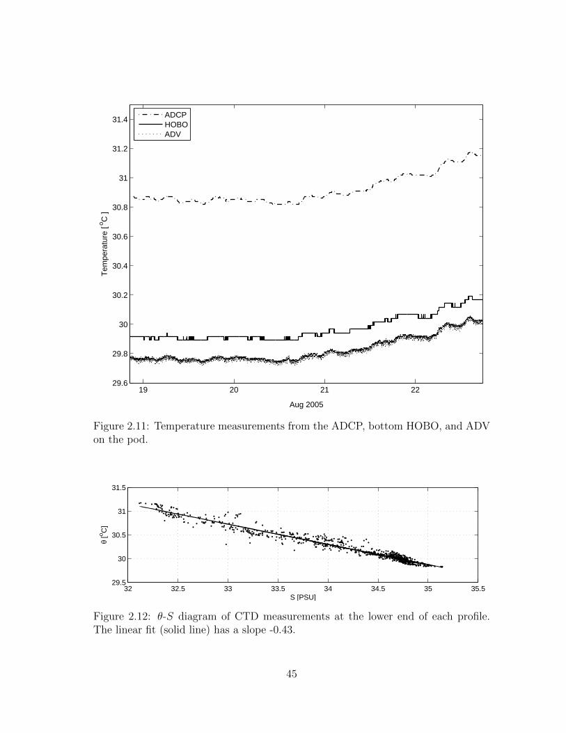
19 20 21 2229.6

29.8

30

30.2

30.4

30.6

30.8

31

31.2

31.4

Aug 2005

Tem

pera

ture

[ o C

]

ADCPHOBOADV

Figure 2.11: Temperature measurements from the ADCP, bottom HOBO, and ADVon the pod.

32 32.5 33 33.5 34 34.5 35 35.529.5

30

30.5

31

31.5

S [PSU]

θ [o C

]

Figure 2.12: θ-S diagram of CTD measurements at the lower end of each profile.The linear fit (solid line) has a slope -0.43.

45

depth of the ADV were estimated according to the linear fit of the θ-S digram of

CTD measurements at each lower end of the profile (Figure 2.12):

θ = 44.79− 0.43S. (2.8)

σθ was then calculated throughout the water column (Figure 2.9c). Values of squared

buoyancy frequency, N2 = −g/ρ0∂zρ (ρ0 is the mean density, and ρ is the density),

indicated the presence of strongly stratified layers within the pycnocline at depths

about 8 and 18 m (Figure 2.9d).

Current velocities were measured from the ADCP, from the surface to 1.24 m

above the bottom, and from the ADV 0.93 m above the bottom. ADCP measure-

ments at the lowest cell were found to be consistent in trend with those from the

ADV (Figure 2.13). Near-surface measurements of the ADCP were contaminated

due to sidelobe interference near the surface (Figure 2.14, Appell et al., 1991; Muste

et al., 2004) and the upper 10% of velocity profiles were, therefore, removed from

the analysis (Figure 2.9e,f). Currents changed directions concurrent with the semi-

diurnal tidal cycles in the v component throughout the water column. Currents in

the SBL (depths above 8 m), mid layer (8 to 19 m) and BBL (19 to 21 m) are de-

scribed as follows in two periods: from late Aug. 18 to late Aug. 20 (period 1) and

from late Aug. 20 to late Aug. 22 (period 2). In the SBL, the mean values of current

speeds decreased from 0.17 m s−1 in period 1 to 0.11 m s−1 in period 2 for both u

and v components. In the mid layer between the strongly stratified layers, the mean

of u was 0.07 m s−1, and the u component dominated, and the mean current speed

increased to 0.2 m s−1. The magnitude of mean v values remained 0.1 m s−1 during

periods 1 and 2. In the BBL, both u and v components were low in magnitude with

mean values of 0.04 m s−1 over the experiment, although the u component showed

46

0

0.2

0.4

0.6

0.8

1

ADV, offset 0 m s−1

ADCP 1st cell, offset 0.36 m s−1

ADCP 2nd cell, offset 0.76 m s−1

u [m

s−

1 ]

0

0.2

0.4

0.6

0.8

1

ADV, offset 0 m s−1

ADCP 1st cell, offset 0.36 m s−1

ADCP 2nd cell, offset 0.76 m s−1

v [m

s−

1 ]

19 20 21 22−0.1

0

0.1

0.2

0.3

0.4

0.5

0.6

0.7

0.8

ADV, offset 0 m s−1

ADCP 1st cell, offset 0.36 m s−1

ADCP 2nd cell, offset 0.76 m s−1

w [m

s−

1 ]

Aug 200519 20 21 22

0

0.2

0.4

0.6

0.8

1

ADV, offset 0 m s−1

ADCP 1st cell, offset 0.36 m s−1

ADCP 2nd cell, offset 0.76 m s−1

curr

ent s

peed

[m s

−1 ]

Aug 2005

Figure 2.13: Velocity measurements from the ADV and the lowest two cells of ADCP.For clarity, the ADCP measurements were offset by 0.36 and 0.76 m s−1 for cells 1and 2, respectively.

47

Figure 2.14: The geometry of ADCP sidelobe interference. RMAX = Hcosα is themaximum range of good data, α = 25 is the angle from the beam to vertical di-rection, hence RMAX = 0.9H. The sidelobe acoustic energy reflected by the sur-face contaminates the near-surface measurements. The green check marks indicategood cells, while measurements in the cells of red cross marks off RMAX is rejected(Aquadopp Current Profiler User Guide, Nortek).

48

little temporal variability compared to the v component. Squared shear frequency,

M2 = (∂zu)2 + (∂zv)2, presented relatively high values (> 0.05 s−2) where strong

u currents showed high vertical gradients in period 2 (Figure 2.9g). Ri = N2/M2

primarily corresponded to N2 (Figure 2.9h), indicating stability in the pycnocline.

2.4.3 Model formulation

Four models were applied for turbulence simulations:

• CH: the k − ε turbulence closure with the stability functions of Cheng et al.

(2002)

• SG: the k − kL turbulence closure with the stability functions of Schumann

and Gerz (1995)

• CHx: the k−kL turbulence closure with the stability functions of Cheng et al.

(2002)

• SGx: the k−ε turbulence closure with the stability functions of Schumann and

Gerz (1995)

Formulations of the stability functions of Cheng et al. (2002) and Schumann and

Gerz (1995) are presented in Appendix B.

In the k − ε turbulence closure, ε is derived from the transport equation

Dε

Dt= Γε +

ε

k(c1εP + c3εB − c2εε) , (2.9)

where DDt

denotes the material derivative, Γ is the sum of the viscous and tur-

bulent transport terms, P is the shear production, B is the buoyancy produc-

tion/destruction, c1ε = 1.44, c2ε = 1.92, and c3ε = 1.

49

In the k − kL turbulence closure, ε is given by

ε =(c0µ)3 k 3

2

L, (2.10)

where c0µ = 0.5477, and L is derived from

D (q2L)

Dt= ΓL + L (E1P + E3B − E2Fε) , (2.11)

where E1 = 1.8, E2 = 1.33, and E3 is a function of Ri and stability functions (Mellor

and Yamada, 1982). The wall function, F , is used to reproduce the logarithmic part

of the law of the wall (Umlauf and Burchard , 2003), and is given by

F = 1 + E2

(L(ds + db)

κdsdb

)2

, (2.12)

where ds is the distance from the sea surface, and db is the distance from the bottom.

The typical velocity scale of turbulence, q, is defined by

k =q2

2, (2.13)

and the transport equation for q is given by

D(q2

2)

Dt= Γq + P +B − ε. (2.14)

To correspond to the observed TKE calculated from equation (2.5), the modeled

TKE was calculated from w′2, which is derived from

w′2

k=

2

3+

1

Ψε

((a23− a3

)P +

8

3a5B

), (2.15)

50

where Ψε = 2.5ε, a2 = 0.016, a3 = 0.432, and a5 = 0.25 for stability functions of

Cheng et al. (2002), while the second term on the right hand side of the equation

is absent for stability functions of Schumann and Gerz (1995), i.e. it simplifies to

equation (2.5). Values of TKE were calculated from equations (2.13) and (2.14) for

the k − kL turbulence closure and from the transport equation

Dk

Dt= Γk + P +B − ε (2.16)

for the k − ε turbulence closure.

The simulated τ for the four models is given by

τ = ρνt|M |, (2.17)

where νt is the eddy viscosity. In the k − ε turbulence closure, νt is given by

νt = cµk2

ε, (2.18)

where cµ is the stability function in Appendix B; in the k − kL turbulence closure,

νt is given by

νt = cµk12L. (2.19)

Since one-dimensional models are generally unable to account for advective effects

(Bolding et al., 2002), a mechanism of ”relaxing” has been implemented in which

modeled values are adjusted according to the observations (Burchard , 1999; Anis

and Singhal , 2006; Burchard et al., 2006; Peters and Baumert , 2007; Cabrillo et al.,

2011). In our simulations, models were relaxed to observed u and v profiles every

4000 s, and θ and S profiles every 360 s. Examinations of several relaxation times and

51

10−9

10−8

10−7

10−6

ε [m

2 s−

3 ]

obsCHSG

10−7

10−6

10−5

10−4

TK

E [m

2 s−

2 ]

10−5

10−4

10−3

10−2

τ [k

g m

−1 s

−2 ]

19 20 21 22

10−1

100

101

102

Ri

Aug 2005 [UTC]

a

b

c

d

Figure 2.15: Comparisons of turbulence quantities computed from observations tothose from the CH and SG models in the BBL: (a) ε, (b) TKE, (c) τ , and (d) Ri

(Rci = 1 is indicated by a horizontal dash-dot line).

the relationship between mean simulated ε values and relaxation times are further

discussed in Appendix C.

2.5 Analysis

ε, TKE, τ , and Ri from observations and models in the BBL are compared in

Section 2.5.1. Comparisons between the four models throughout the water column

are discussed in Section 2.5.2.

52

min max mean [95%CI]obs 5.99e-9 1.21e-6 1.87e-7 [1.75e-7 2.02e-7]

ε [m2 s−3] CH 1.20e-8 1.18e-6 2.41e-7 [2.30e-7 2.53e-7]SG 8.19e-9 1.10e-6 2.10e-7 [1.99e-7 2.21e-7]obs 1.45e-6 1.12e-4 2.91e-5 [2.76e-5 3.06e-5]

TKE [m2 s−2] CH 1.43e-6 7.35e-5 1.63e-5 [1.57e-5 1.71e-5]SG 1.34e-6 7.87e-5 1.81e-5 [1.74e-5 1.90e-5]obs 1.96e-3 5.04e-2 1.51e-2 [1.44e-2 1.59e-2]

τ [kg m−1 s−2] CH 3.05e-4 3.13e-2 6.09e-3 [5.77e-3 6.38e-3]SG 3.86e-4 2.65e-2 6.10e-3 [5.84e-3 6.40e-3]obs 4.62e-2 61.05 3.00 [2.73 3.36]

Ri CH 1.51e-1 2.79 0.53 [0.52 0.55]SG 1.23e-1 6.71 1.03 [1.00 1.06]

Table 2.2: Minima, maxima, mean values, and 95% confidence intervals for ε, TKE,τ , and Ri for the observations, and the CH and SG models. Simulated TKE valuesless than 1.5 times vertical noise energies were discarded according to equation (2.5),and the corresponding points were removed for other modeled quantities as well.

2.5.1 Observation-model comparisons in the BBL

Turbulence quantities (ε, TKE, and τ) and Ri from the observations and the

CH and SG models are shown in Figure 2.15. Simulation results of the CH and

SG models were nearly identical such that the lines of the models were primarily

superimposed. The trends of modeled ε and TKE followed those observed, however,

there were occasions when model values were much low. In most of these cases,

the power spectrum was consistently lacking a clear inertial subrange, so that the

Kolmogorov’s hypothesis could not be applied and ε was not estimated. In particular,

the simulated τ was substantially lower than the measured τ .

For their statistics (Table 2.2), values of vertical noise energy (9.53×10−7 m2 s−2

on average) in all bursts were interpolated to time points of simulations, and any

simulated TKE value, according to equation (2.5), less than 1.5× the corresponding

vertical noise energy in each burst was discarded. Values of simulated ε, τ , and Ri at

53

corr(obs, CH) [95%CI] corr(obs, SG) [95%CI] corr(CH, SG) [95%CI]ε 0.31 [0.24 0.38] 0.33 [0.25 0.40] 0.99 [0.99 0.99]

TKE 0.48 [0.41 0.53] 0.48 [0.43 0.53] 0.99 [0.99 1.00]τ 0.36 [0.31 0.42] 0.32 [0.25 0.37] 0.99 [0.99 0.99]

Table 2.3: Cross-correlations and 95% confidence intervals between the observationsand the CH and SG models for ε, TKE, and τ .

the same time point were filtered out accordingly as well. Minimal, maximal, mean

values, and their 95% confidence intervals for ε, TKE, and τ from the two models

were similar to those from observations.

Mean Ri values computed from the observations were similar to those from the

CH and SG models. A flow is commonly considered stable if Ri is greater than a

critical gradient Richardson number (Rci ). Although there is no unique value for

Rci , in laboratory and field work, estimates of Rc

i are on the order of 1 (Gerz et al.,

1989; Jacobitz et al., 1997; Kundu and Cohen, 2008). Here, 42% of the observed

Ri values were found to be less than Rci = 1, compared to 43% for those computed

from the CH model, and 84% for those computed from the SG model. Turbulence

in the BBL was active most of the time. During stable conditions in the BBL,

e.g., when values of observed Ri >5, model predicted Ri values deviated from the

observations, indicating that the models may inaccurately predict the evolution of

turbulence under such stable conditions (Baker and Gibson, 1987; Burchard et al.,

2002).

Model simulated values of ε, TKE, and τ were linearly interpolated to time of the

observed estimations, and scatter plots of observed and modeled values are presented

in Figure 2.16 together with linear fits (calculated using the RR). All slopes of the

linear fits were<1 due to the general lower values from model simulations. Differences

between the CH and SG model simulations were within a factor of 2.

54

10−8

10−7

10−6

ε CH

[m2 s

−3 ]

10−8

10−7

10−6

10−8

10−7

10−6

εobs

[m2 s−3]

ε SG

[m2 s

−3 ]

10−6

10−5

10−4

TK

EC

H [m

2 s−

2 ]

10−6

10−5

10−4

10−6

10−5

10−4

TKEobs

[m2 s−2]

TK

ES

G [m

2 s−

2 ]

10−3

10−2

τ CH

[m2 s

−2 ]

10−3

10−2

10−3

10−2

τobs

[m2 s−2]

τ SG

[m2 s

−2 ]

a

b

c

d

e

f

slope = 0.317

slope = 0.278

slope = 0.219

slope = 0.385

slope = 0.207

slope = 0.237

Figure 2.16: Scatter plots (log scales) for the observations (abscissas) and the CHand SG models (ordinates) for ε (a, b), TKE (c, d), and τ (e, f). Linear fits werecalculated using the RR and are represented by the solid lines.

min max mean [95%CI]ε [m2 s−3] CHx 1.44e-8 1.95e-6 4.10e-7 [3.90e-7 4.29e-7]

SGx 9.71e-9 1.19e-6 2.36e-7 [2.24e-7 2.48e-7]TKE [m2 s−2] CHx 1.48e-6 1.86e-4 3.47e-5 [3.30e-5 3.66e-5]

SGx 1.27e-6 1.02e-4 2.19e-5 [2.09e-5 2.29e-5]

τ [kg m−1 s−2] CHx 1.46e-4 8.49e-2 1.39e-2 [1.32e-2 1.47e-2]SGx 3.70e-4 3.48e-2 7.30e-3 [6.95e-3 7.66e-3]

Ri CHx 1.68e-1 11.44 0.66 [0.64 0.69]SGx 1.42e-1 6.70 1.14 [1.10 1.18]

Table 2.4: Minima, maxima, and mean values with 95% confidence intervals for ε,TKE, τ , and Ri for the cross-combined models CHx and SGx. Simulated TKE valuesless than 1.5 times vertical noise energies were discarded according to equation (2.5).Corresponding points were removed for other modeled quantities as well.

55

Figure 2.17: Ratios of SG model values to CH model values for (a) TKE obtainedfrom transport equations (2.14) and (2.16), (b) ε, (c) τ , and (d) Ri.

Cross-correlations between the observed and modeled values were all above 46%

(Table 2.3). Not surprisingly, the CH and SG models correlated highly for any quan-

tity (∼ 98%), given that the models consistently predicted similar trends. Statistics

of the cross-combined models (CHx and SGx) were similar to those of the CH and

SG models (Table 2.4).

2.5.2 Inter-model comparisons throughout the water column

Comparisons between the CH, SG, CHx, and SGx models were made throughout

the water column. Here, calculations of TKE were not restricted to the vertical

56

velocity component in equation (2.5). Instead, they were simulated from transport

equations (2.14) and (2.16) for the k−kL and k− ε turbulence closures, respectively.

Values are equivalent to those given by equation (2.4) in which u′2, v′2, and w′2 were

taken into account. Ratios of TKE, ε, τ , and Ri from the SG to CH models are

shown in Figure 2.17. The two models agreed well in the SBL and BBL, but the

SG model estimated turbulence quantities greater values than the CH model in the

pycnocline, particularly for τ that exhibited ratios >3 (Figure 2.17c).

Parameters on the right hand sides of TKE transport equations (2.14) and (2.16)

are compared in Figure 2.18. The sum of shear and buoyancy production rates

(P +B) is close to TKE dissipation rate (ε), such that:

Γ

P +B − ε 1. (2.20)

where Γ represents Γq in equation (2.14) and Γ represents Γk in equation (2.16).

Thus, Γ is the main factor determining the rate of change in TKE transport equations

(2.14) and (2.16) denoted as Γq and Γk, respectively. Ratios (Γq/Γk) in Figure 2.18a

showed similar patterns to those for TKE in Figure 2.17a. P and B are given by

P = νtM2 (2.21)

and

B = −ν ′tN2, (2.22)

where ν ′t is the eddy diffusivity. Both P (Figure 2.18b) and B (Figure 2.18c) values

in the pycnocline were estimated to be greater in the SG model, because νt (Figure

2.18d) and ν ′t (Figure 2.18e) were overestimated, showing ratios higher than 1, while

ratios of M2 (Figure 2.18f) and N2 (Figure 2.18g) were ∼1.

57

Figure 2.18: Ratios of SG model values to CH model values for (a) Γq/Γk, (b) P , (c)B, (d) νt, (e) ν ′t, (f) M2, and (g) N2.

58

Figure 2.19: Ratios of τ values between the models: (a) SG/CHx; (b) SGx/CH; (c)SG/SGx; (d) CHx/CH.

59

It is not clear whether the turbulence closures or the stability functions were

responsible for the differences in the pycnocline between the models results. To

investigate this further, the turbulence closures and the stability functions were cross-

combined for the CHx and SGx models. Figures 2.19a and 2.19b indicate that for

the same turbulence closures, the stability functions of Schumann and Gerz (1995)

resulted in higher τ values (τSG > τCHx and τSGx > τCH); Figures 2.19c and 2.19d

indicated that for same stability functions, either the k − ε or k − kL turbulence

closure resulted in similar τ values (τSG ≈ τSGx and τCHx ≈ τCH). Thus differences

between the four models appear to be mainly caused by the stability function. This

is suggested from equations (2.17), (2.18), and (2.19) that cµ is the main factor for

τ .

2.5.3 Influence of surface fluxes on turbulence in the BBL

Stratification was prevalent during the experiment, it suppressed vertical mixing.

The strong wind event at site D deepened the mixed layer (Figure 2.9a, b, c), e.g.

the depth of σθ = 18 kg m−3 was deepened 1.88 m in 87 minutes after 02:00, and

was forceful enough to affect BBL currents, resulting in the maximum of observed

current magnitude (Figure 2.7b) and a consequent increase in ε values. To inves-

tigate the influence of surface meteorological forcing on the dynamics in the BBL,

the four models were run without the input of surface heat and momentum fluxes.

These simulations revealed that mixing was effectively damped in the SBL, however,

turbulence dynamics did not change in the BBL most likely due to the strong strati-

fication in the pycnocline except that the BBL current velocity increases induced by

the strong wind vanished.

60

2.6 Discussion

The simplified stability functions of Schumann and Gerz (1995) were found to

be as capable as those of Cheng et al. (2002) for modeling turbulence in the BBL

in our study, but deviated for cµ related quantities, e.g. τ , P , B, νt, and ν ′t, in the

pycnocline. We found no other comparisons of the stability functions of Schumann

and Gerz (1995) to those of Cheng et al. (2002) in the literature. However, there

are studies between the stability functions of Schumann and Gerz (1995) and other

stability functions, e.g. those of Canuto et al. (2001), which can be found in e.g.

Burchard et al. (2002) and Simpson et al. (2002). Canuto et al. (2001) improved the

Mellor-Yamada model with a down-gradient approximation for third-moments. We

tested models with the stability functions of Canuto et al. (2001), and the results (not

shown) presented minor differences from the models applying the stability functions

of Cheng et al. (2002). Applications of the stability functions of Canuto et al. (2001)

are described as follows, from which we try to explain the discrepancy between the

stability functions of Cheng et al. (2002) and Schumann and Gerz (1995).

Burchard et al. (2002) tested the k− ε turbulence closure with the stability func-

tions of Canuto et al. (2001) and Schumann and Gerz (1995) throughout a water

column with a depth of 110 m. Results of their two models were found to be similar,

and both agreed with observations when the water was stably stratified. In an area

strongly influenced by horizontal temperature and salinity gradients, tidal straining,

and vertical mixing, Simpson et al. (2002) applied two models by combining the

k − ε turbulence closure with the stability functions of Canuto et al. (2001) and

Schumann and Gerz (1995), respectively, throughout a water column with a depth

of 35 m. Results from the former model agreed well with those from observations,

while the latter model predicted a lower ε maximum. From the two studies above,

61

it appears that the comparison results are not consistent under different scenarios,

however, the stability functions of Schumann and Gerz (1995) have less dependence

on buoyancy through a constant and the turbulent Prandtl number (Simpson et al.,

2002), which might yield inconsistency to complex stability functions e.g. of Cheng

et al. (2002), especially in the pycnocline. The simulations in Peters and Baumert

(2007) also indicated that the stability functions of Schumann and Gerz (1995) were

not able to simulate observed turbulence in stably stratified flows.

Several studies have shown that all length scale related equations perform equiva-

lently for stress-dominated boundary layer flows when properly calibrated (e.g., Bur-

chard et al., 1998; Baumert and Peters , 2000; Burchard , 2001a). Applying steady-

state Richardson numbers to B by Burchard (2001a) for the k−kL turbulence closure

and by Burchard and Baumert (1995) for the k−ε turbulence closure gave equivalent

results. In full-equilibrium flows ( DDt

= 0), the k − kL and k − ε turbulence closures

were found to be interchangeable by setting cε3 = 1 in equation (2.9) without any

loss of generality (Baumert and Peters , 2000). However, the study of Burchard et al.

(1998) showed that two-equation models are more sensitive to the choice of stabil-

ity functions than turbulence closures. This is consistent with the present study’s

findings.

2.7 Conclusions

The water column on the Texas-Louisiana continental shelf was strongly strati-

fied and wind speeds were moderate most of the time. Surface heat and momentum

fluxes were found to have little effect on turbulence in the BBL, with the pycno-

cline effectively suppressing vertical mixing, and inhibiting transport of waterborne

constituents such as nutrients, oxygen, etc. A single, short, strong wind event deep-

ened the mixed layer and affected currents in the BBL. This resulted in the u in the

62

BBL reaching a maximum during the wind event. Turbulence was not active near

the bottom over the experiment, with only 32.6% burst measurements presented a

clear inertial subrange in energy spectra of vertical velocity fluctuations. Turbulence

quantities (ε, TKE, and τ) in the BBL were studied using observational and mod-

eling methods, and meteorological data from various sources near and at the study

site were obtained for model simulations.

Vertical velocities measured from the ADV were applied to estimate ε, TKE, and

τ due to the lower noise level of the vertical component compared to the horizontal

components, as well as the less impact of surface wave induced motions in the vertical

direction than in the horizontal directions. Observed ε values were estimated in

inertial subranges of energy spectra following Kolmogorov’s -5/3 law with the removal

of surface wave effect introduced by Trowbridge and Elgar (2001). ε values from this

method were lower than those from the original energy spectrum equation (2.1) with

a factor 0.44. Magnitudes of observed ε were strongly affected by v, following the

trend of velocity magnitudes in the BBL. Observed TKE values were calculated by

integrating spectra under the logarithmic fits in inertial subranges, and observed τ

values were calculated from the ε estimates according to the law of the wall.

Four numerical models (CH, SG, CHx, and SGx) were applied for turbulence

simulations in the BBL, using combinations of turbulence closures (k−ε and k−kL)

and stability functions (Cheng et al., 2002 and Schumann and Gerz , 1995). The

models were relaxed to θ, S, u, and v measurements, correcting advection to these

quantities. The trends of ε, TKE, and τ for the four models were consistent with

observations, and their mean values were similar to those observed. After comparing

the measurements at another mooring site with a similar water depth, as well as

the verification by the observation-model comparisons, it was suggested that the

assumption of homogeneous salinity in the BBL was appropriate. Modeled TKE

63

values were computed using two methods: 1) equation (2.5) and modeled vertical

velocity variances for observation-model comparisons; 2) transport equations (2.14)

and (2.16) for inter-model comparisons. Results from both methods showed similar

TKE values between the SG and CH models in the BBL. Analyses of each parameter

on the right hand side of the transport equations revealed that Γ was the major factor

to the temporal variability of TKE. The CH, SG, CHx, and SGx models performed

analogously in the BBL, while differences between the models in the pycnocline were

found to be primarily caused by the stability functions rather than the turbulence

closures.

Although second-moment two-equation statistical turbulence closure models have

been widely used for comparisons in the entire water column, a relatively small

number of studies have been carried out at specific depth intervals (Burchard et al.,

2002; Wang et al., 2011). The present study provides new insight on the turbulence

dynamics in the BBL and the applicability of turbulence models to simulate the

dynamics in these layers on the continental shelf.

64

3. OBSERVATIONS AND MODEL SIMULATIONS OF TURBULENCE IN A

HYPOXIC ZONE WITH THE ADVECTION OF NON-LOCAL WATER

3.1 Introduction

A field campaign was conducted on the continental shelf of the Gulf of Mexico

in the summer of 2005 when hypoxia prevailed. One of the major objectives for this

campaign was to study vertical mixing processes in the hypoxic zone. Vertical mixing

is a key factor in controlling biogeochemical fluxes in the ocean, and it is driven by

two major processes: divergent Ekman transport and turbulent mixing (Cuypers

et al., 2011). The latter is perhaps the most important and responsible for the

downward supply of oxygen through the pycnocline and upward supply of nutrient

from the bottom boundary layer (BBL), thus it needs to be accurately quantified in

order to adequately represent biogeochemical processes (Klein and Lapeyre, 2009).

Wind stress is the main source for mixing in the surface boundary layer (SBL) in the

summer, while shear due to friction is responsible for the mixing in the BBL (Palmer

et al., 2013). Internal waves and shear advection may furthermore account for the

dynamics in stratified layers between the SBL and BBL (Thorpe, 2004).

The present study, through a combined observational and modeling effort, aims to

improve the understanding of turbulence dynamics and the influence of turbulence on

hypoxia. Turbulence can be studied from direct measurements of the vertical turbu-

lent fluxes, e.g. momentum fluxes (u′w′ and v′w′), heat flux (θ′w′), and salinity flux

(S ′w′), but more often, turbulence quantities are examined as indirect measurements

of turbulence. Turbulence quantities include, e.g. dissipation rate of temperature

variance (χ), dissipation rate of turbulence kinetic energy (ε), eddy diffusivity of tem-

perature (ν ′t), and eddy diffusivity of density (ν ′ρ). Turbulent processes have been

65

investigated in terms of these quantities in many studies (e.g. Anis , 2006; Anis and

Singhal , 2006; Cousins et al., 2010; Cuypers et al., 2011). In the present study, turbu-

lence dynamics throughout the water column were investigated using measurements

of temperature and salinity microstructure, as well as the current profiles in the lower

part of the water column. χ, ε, ν ′t, and ν ′ρ were estimated from observational meth-

ods as follows. χ was calculated from the integral of the energy spectra of vertical

temperature gradient (∂zθ), and ε was then derived from a Batchelor fit to the en-

ergy spectra (Batchelor , 1959; Oakey , 1982; Ruddick et al., 2000). ν ′t was calculated

from the product of χ and (∂zθ)2 (Oakey , 1982; Anis and Singhal , 2006), and ν ′ρ was

estimated as a function of ε and buoyancy frequency squared (N2 = − gρ0

∂ρ∂z

, where ρ0

is the mean density; Ivey et al., 2008). Further details of observational methods for

the four turbulence quantities are given in Section 3.3. Turbulent oxygen flux was

estimated throughout the water, and the time required to remove bottom hypoxic

layer by turbulence was calculated.

Two-equation second-moment turbulence models have been widely applied in

turbulent mixing studies (Umlauf and Burchard , 2005). They consist of two transport

equations: one for turbulence kinetic energy (k) and the other for a length scale

(L) related quantity (e.g. ε or kL). This type of models has been applied for

studies for an individual model with different parameterizations (Burchard , 2001b;

Bolding et al., 2002), comparisons between models (Burchard , 2001a; Burchard et al.,

2006, 2008), and comparisons between observations and models (Anis and Singhal ,

2006; Zhang and Drennan, 2012). In the present study, the k − ε and k − kL

turbulence closures models were applied to simulate χ, ε, ν ′t, and ν ′ρ for comparisons

to observations. Turbulence theories and numerical models are commonly based on

the assumption of locality (Mellor and Yamada, 1982; Rodi , 1987), but very often

turbulence is influenced by non-local processes, such as advection (Burchard , 1999;

66

Anis and Singhal , 2006; Burchard et al., 2006; Cabrillo et al., 2011). Here, advection

was accounted for by relaxing the simulations to the measured potential temperature

(θ) and salinity (S).

The paper is structured as follows: after describing the study site (Section 3.2.1),

the surface forcing (Section 3.2.2) and hydrography (Section 3.2.3) used for model

simulations are presented. Advection of non-local water over the hypoxic layer is

described in the context of the relatively high turbulence levels observed (Section

3.2.4). An introduction to observational methods is given in Section 3.3, followed by

estimation of turbulent oxygen flux according to observed ν ′ρ (Section 3.4). A short

description of the numerical models is given in Section 3.5. Observational and model

results are compared for χ and ε in Section 3.6.1 and for ν ′t and ν ′ρ in Section 3.6.2.

Discussion and conclusions are presented in Sections 3.7 and 3.8, respectively.

3.2 Experimental details

3.2.1 Study site

The study site C (Figure 3.1) is on the continental shelf of the Gulf of Mexico,

60 km south of the coast at 2856′55′′N 9157′5′′W, and has a water depth of 21.5

m. The campaign at site C was part of the NOAA Mechanisms Controlling Hypoxia

(MCH) project (http://hypoxia.tamu.edu), and was conducted for 24 h from Aug.

22 20:00 to Aug. 23 20:00 (UTC = CDT + 5 h) during hypoxic conditions (Rabalais

et al., 2007).

3.2.2 Surface forcing

Momentum flux, τwind, was calculated from wind speeds measured at the near-

est available source the National Data Buoy Center station LUML1 (2915′12′′N

9039′48′′W, Figure 3.1). During the field study, the weather was clear, and observed

wave heights were less than 0.3 m. Meteorological conditions were characterized by

67

Figure 3.1: The measurements were conducted at site C on the Texas - Louisianacontinental shelf. Net longwave radiation from NCEP was interpolated to site C;downward shortwave radiation was observed at fire station McFaddin; LUML1 buoystation that provided the rest of meteorological data required for calculations ofsurface heat and momentum fluxes. Velocity measurements were rotated to along-shelf (u) and cross-shelf (v) directions as presented by the axis system on the figure.Site D, about 150 km west of site C, included a bottom-mounted upward lookingacoustic Doppler current profiler (ADCP).

low to moderate wind speeds with the average 2.8 m s−1 and the maximum 6.2 m s−1

(Figure 3.2a), resulting in τwind < 0.06 N m−2 (Figure 3.2b).

Net surface heat flux, J0q , was computed as the sum of four components:

J0q = Jswq + J lwq + J lq + Jsq (3.1)

where Jswq is the net shortwave radiation, J lwq is the net longwave radiation, J lq is

the latent heat flux due to evaporation/condensation, and Jsq is the sensible heat

flux. Jswq was calculated from the measurement of incoming solar radiation at the

US Forest Service weather station McFaddin (2942′0′′N 947′0′′W, Figure 3.1), ap-

plying an albedo correction using the formula in Payne (1972). J lwq was computed

from the sea surface temperature (SST) and downward longwave radiation following

Dickey et al. (1994). The SST (Figure 3.2b) was obtained from profiles taken by a

68

−6

−4

−2

0

2

4

Win

d ve

ctor

[m s

−1 ]

31.4

31.5

31.6

31.7

31.8

31.9

32

SS

T [o C

]

22:00 2:00 6:00 10:00 14:00 18:00−400

−200

0

200

400

600

800

J q0 [W m

−2 ]

Aug 23 2005 [UTC]

0

0.01

0.02

0.03

0.04

0.05

0.06

τ win

d [N m

−2 ]

a

b

c

Figure 3.2: Meteorological measurements: (a) hourly wind vector; (b) sea surfacetemperature; (c) heat flux, Joq (black), and momentum flux, τwind (gray).

69

Self Contained Autonomous MicroProfiler (SCAMP, Precision Measurement Engi-

neering). The downward longwave radiation was retrieved from the National Centers

for Environmental Prediction/Department of Energy Reanalysis 2 (NCEP) database

(Sun et al., 2003; Kubota et al., 2008), and interpolated to site C. J lq and Jsq were cal-

culated using wind speed, air temperature, relative humidity and air pressure from

LUML1, and SST (Fairall et al., 1996). During the period of the experiment, J0q

varied between -400 and 800 W m−2 (Figure 3.2c).

3.2.3 Hydrography

Vertical structures of temperature, salinity, and density were revealed from the

SCAMP measurements. The SCAMP sensors include an accurate conductivity sen-

sor, a fast conductivity sensor, two fast thermistors, and a pressure sensor (MacIntyre

et al., 1999; Jurado et al., 2012). Downward profiles of temperature, small-scale verti-

cal temperature gradients (∂zT ), conductivity, and pressure were taken every ∼7 min

while this instrument fell freely at a speed ∼ 0.1 m s−1. Measurements started at ∼

1 m below the surface and reached down to the seafloor. Measurements of accurate

conductivity were chosen for calculations because signals from the fast conductivity

sensor were contaminated. Measurements from the two fast thermistors were in good

agreement, thus one of the two measurements were chosen for the calculations.

Profiles of θ, S, and σθ, shifted by 0.3 units and aligned with time and sea

surface elevations, are presented in Figure 3.3. The SBL (BBL) of θ was marked by

black dots where the temperature is 0.1 oC lower (higher) than that at the surface

(bottom) in each profile (Figure 3.3b). The SBLs and BBLs of S and σθ were defined

analogously but with the vertical differences 0.1 PSU and 0.1 kg m−3, respectively

(Figure 3.3c, d). The mean depth of SBL of σθ (6.07 m) was same as that of S and

1.9 m shallower than that of θ, while the mean depth of BBL of σθ (18.11 m) was

70

22:00 2:00 6:00 10:00 14:00 18:0021

21.1

21.2

21.3

21.4

surf

ace

elev

. [m

]

30 40 50 60 70 80 90

−20

−15

−10

−5

0

θ [oC]

Dep

th [m

]

30 40 50 60 70 80 90

−20

−15

−10

−5

0

S [PSU]

10 20 30 40 50 60 70 80

−20

−15

−10

−5

0

σθ [kg m−3]

a

b

c

d

Figure 3.3: (a) surface elevation; SCAMP profiles of (b) θ, (c) S, and (d) σθ. TheSBLs and BBLs defined in θ (b), S (c), and σθ (d) profiles are marked by black dotswhere the values are 0.1 units different than those at the surface and at the bottom,respectively. Profiles are offset by 0.3 units and aligned with the time in (a). Timeintervals between profiles are ∼ 7 min.

71

Figure 3.4: Contours from SCAMP profiles at site C: (a) potential temperature, θ;(b) salinity, S; (c) σθ; (d) buoyancy frequency squared, N2. The SBLs and BBLsdefined in θ (a), S (b), and σθ (c, d) are marked by white dots.

72

Figure 3.5: Ship hull-mounted ADCP velocity contours between depths 12.4 and18.4 m at site C: (a) along-shelf velocity, u; (b) cross-shelf velocity, v; (c) currentspeed; (d) current direction (0 is the along-shelf direction and angles increase counter-clockwise). The BBL defined in σθ is marked by white dots.

1.53 m below that of S and 0.7 m above that of θ. An enhanced mixing section

in density profiles is shown between 10 and 18 m from 2:00 to 5:00 (Figure 3.3d).

The mixing was caused by rapid changes in both measured θ and S (Figure 3.3b, c),

which elevated the depth of SBL of θ at the top of the mixing section (Figure 3.4a).

Below the SBL of σθ, N2 presented high values, indicating the pycnocline (Figure

3.4d). In the following study, we denote the SBL, mid layer, and BBL as defined in

σθ profiles unless they are specified otherwise.

Velocity profiles were measured from a ship (R/V Gyre) hull mounted Teledyne

RD Instruments 150 kHz acoustic Doppler current profiler (ADCP). Eastward and

northward velocities were rotated 15o clockwise to along-shelf (u) and cross-shelf

(v) directions (Figure 3.1). Measurements started at a depth of 12.4 m, with a bin

size of 2 m and an interval of 5 min (Figure 3.5a, b). Data deeper than 18.4 m were

discarded due to side-lobe contamination from bottom echoes (Nystrom et al., 2002).

73

Figure 3.6: Current measurements: along-shelf velocities at site C (a) and D (b);cross-shelf velocities at site C (c) and D (d). A white line at 12.4 m was addedon panels b and d to indicate the start depth of current measurements at site C.Currents at site D were measured from an upward looking ADCP (Nortek 1 MHzAquadopp).

74

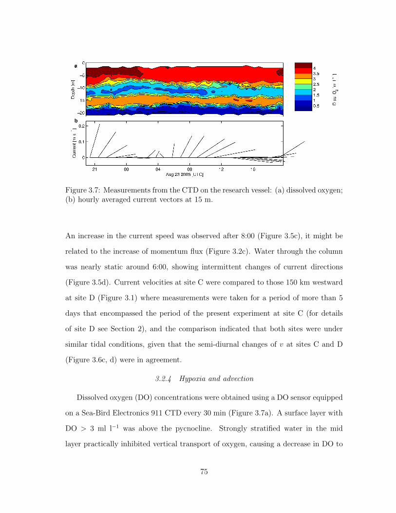
Figure 3.7: Measurements from the CTD on the research vessel: (a) dissolved oxygen;(b) hourly averaged current vectors at 15 m.

An increase in the current speed was observed after 8:00 (Figure 3.5c), it might be

related to the increase of momentum flux (Figure 3.2c). Water through the column

was nearly static around 6:00, showing intermittent changes of current directions

(Figure 3.5d). Current velocities at site C were compared to those 150 km westward

at site D (Figure 3.1) where measurements were taken for a period of more than 5

days that encompassed the period of the present experiment at site C (for details

of site D see Section 2), and the comparison indicated that both sites were under

similar tidal conditions, given that the semi-diurnal changes of v at sites C and D

(Figure 3.6c, d) were in agreement.

3.2.4 Hypoxia and advection

Dissolved oxygen (DO) concentrations were obtained using a DO sensor equipped

on a Sea-Bird Electronics 911 CTD every 30 min (Figure 3.7a). A surface layer with

DO > 3 ml l−1 was above the pycnocline. Strongly stratified water in the mid

layer practically inhibited vertical transport of oxygen, causing a decrease in DO to

75

between 1.5 and 3 ml l−1 below the pycnocline. A layer of high-concentration DO (≥

3 ml l−1) water occurred between 14 and 18 m. Hourly averaged current velocities

at 15 m were primarily east or northeast (Figure 3.7b), indicating the advection of

non-local water. Hypoxia is defined as DO < DOc = 1.4 ml l−1 (critical value) and

was present near the bottom, it corresponded to the pycnocline near the BBL (Figure

3.4d) which kept DO from transporting downward.

3.3 Observational methods

ε was calculated based on the theoretical Batchelor spectrum (Batchelor , 1959;

Dillon and Caldwell , 1980; Oakey , 1982; Imberger and Ivey , 1991) and given by

ε = k4Bνν2T , (3.2)

where ν = 8×10−7 m2 s−1 is the kinematic viscosity at 30C, νT = 1.4×10−7 m2 s−1

is the thermal diffusivity, and kB is the Batchelor cutoff wavenumber estimated from

the Batchelor spectrum:

E(kwn) =(q

2

) 12 χ

kBνTg(q, kwn/kB), (3.3)

where q = 3.4 was chosen in this study (Grant et al., 1968; Dillon and Caldwell ,

1980; Ruddick et al., 2000), and g(q, kwn/kB) is given by

g(q, kwn/kB) = 2π

(e−α

2/2 − α∫ ∞α

e−x2/2dx

), (3.4)

where kwn = kwn/2π is the cyclic wavenumber, and

α = (2q)12

2πkwnkB

. (3.5)

76

χ is given by

χ = 6νT (∂zθ′)2 = 6νT

∫ ∞t

(Eobs(kwn)− En(kwn)

)dkwn, (3.6)

where θ′ is the potential temperature fluctuation, Eobs is the observed spectrum of

(∂zθ′)2, and En is the instrument’s noise spectrum. Spectra of (∂zθ′)2 were calcu-

lated for segments in which turbulence was determined to be statistically stationary

(Imberger and Ivey , 1991; Chen et al., 2002), and χ was estimated by integrating the

spectra of each segment. The best fit of Batchelor spectrum of the observed spec-

trum was estimated using the Maximum likelihood algorithm introduced by Ruddick

et al. (2000).

A profile in the enhanced mixing section (Figure 3.8a) was compared to another

in a calm condition (Figure 3.8c). The variation of ∂θ/∂z in the first profile was

∼ 4 times that in the second profile, while temperatures were in the same range.

∂θ/∂z from the first profile indicated strong turbulence activity in the mid layer (7.6

∼ 18.1 m). χ and ε (Figure 3.8b) estimated from the measurements in the segment

between 7.9 and 8.4 m (marked by two horizontal dashed lines, Figure 3.8a) in the

first profile were at least 2 orders of magnitude higher than those (Figure 3.8d) from

the measurements in the segment between 18.8 and 19.4 m (marked by two horizontal

dashed lines, Figure 3.8c) in the second profile.

ν ′t is given by

ν ′t =χ

2

(∂T

∂z

)−2, (3.7)

and ν ′ρ is given by

ν ′ρ = Γε

N2, (3.8)

where Γ = 0.2 is the mixing efficiency (Osborn, 1980; Moum, 1996; Nash et al., 2007).

77

Figure 3.8: (a) an example of a high turbulence energy profile taken at 3:22:00, show-ing potential temperature, θ (black), and vertical gradient of potential temperature,∂zθ (gray); (b) observed spectra (solid line) and fit (dashed line) of a theoreticalBatchelor spectrum for the profile segment (7.9 - 8.4 m) marked by two dashed hor-izontal lines in (a). SCAMP’s noise level is shown by the dotted line; (c) similarto (a) but for a relatively low turbulence energy profile taken at 11:08:38. Note thescale for ∂θ/∂z is smaller than that in (a) by a factor of 4; (d) observed spectra andfit for the profile segment between 18.8 and 19.4 m marked by two dashed horizontallines in (c).

78

Figure 3.9: Turbulent oxygen flux, O′2w′, throughout the water column. Positive

(negative) values indicate upward (downward) fluxes.

3.4 Turbulent oxygen flux

Turbulent oxygen flux is given by

O′2w′ = −ν ′ρ

∂O2

∂z(3.9)

High DO in the SBL resulted in downward flux (Figure 3.9), and DO in the non-

local water was transferred upward and downward to relative low DO water. To

replenish oxygen to DO = DOc in the bottom hypoxic layer, the time (tO2) required

was estimated by

−O′2w′tO2

hO2

= |DOc −DO|, (3.10)

where O′2w′ = 4.76 × 10−6 m ml l−1 s−1 is the average turbulent oxygen flux in the

bottom hypoxic layer, hO2 = 4.38 m is the thickness of the layer, DOc = 1.4 ml l−1,

DO = 0.73 ml l−1 is the average DO in the layer. Thus tO2 ≈ 7.11 days.

In the relatively low-DO layer (DO ≤ 2 ml l−1) between 6 and 15 m, vertically

averaged DO (Figure 3.10a) was not consistent with the turbulent oxygen flux (Figure

3.10b), which indicate that DO was not primarily affected by the oxygen flux but by

stratification and shear stress, although the increase of DO, from 1.6 to 2.5 ml l−1

79

1.5

2

2.5

3

DO

[ml l

−1 ]

22:00 2:00 6:00 10:00 14:00 18:000

0.2

0.4

0.6

0.8

1

Aug 23 2005 [UTC]

105×O

′ 2w

′[m

mll−

1s−

1]

a

b

Figure 3.10: (a) vertically averaged dissolved oxygen in the water within the twolayers of DO = 2 ml l−1 between depths of 6 and 15 m; (b) sum of the turbulentoxygen fluxes at the layers.

after 11:00, might be related to the turbulent oxygen flux.

3.5 Model methods

The one-dimensional water column General Ocean Turbulence Model (GOTM;

Burchard et al. 1999) was used in the present study. The GOTM provides choices

for different types of turbulence closures and stability functions (cµ and c′µ), and has

been successfully applied to reproduce turbulence in different physical scenarios, e.g.

tidal straining (Simpson et al., 2002), stratification (Burchard , 2002), near-bottom

dense inflow (Arneborg et al., 2007), convection in a lake (Stips et al., 2002), and near

surface turbulence (Stips et al., 2005). As a physical model, the modular structure

of GOTM makes it possible to couple with biogeochemical models (e.g. ecosystem,

Burchard et al. 2006; Molen et al. 2012).

Two model combinations in the GOTM were applied for the following part of

this study:

80

• CH: the k − ε turbulence closure with the stability functions of Cheng et al.

(2002);

• SG: the k − kL turbulence closure with the stability functions of Schumann

and Gerz (1995).

The CH and SG models estimate turbulent fluxes as functions of a turbulent diffu-

sivity and a gradient of mean water property:

u′w′ = −νt ∂u∂z , (3.11)

v′w′ = −νt ∂v∂z , (3.12)

T ′w′ = −ν ′t ∂T∂z , (3.13)

S ′w′ = −ν ′t ∂S∂z , (3.14)

where νt is the eddy diffusivity of momentum. For further details of the two models

and the equations for ε, see Section 2. In both models, χ is given by equation (3.7)

in which ν ′t is derived from

ν ′t = c′µk12L, (3.15)

while ν ′ρ is calculated from equation (3.8) in both models.

The CH and SG models were forced by the observed meteorological surface forc-

ing, i.e. heat and momentum fluxes. In addition, they were relaxed to observed θ and

S profiles every 300 s so that simulations did not deviate much from measurements

due to advection (Anis and Singhal , 2006; Cabrillo et al., 2011). No relaxation to

observed velocities was used due to the low vertical resolution of velocity measure-

ments.

81

109χ [oC s−1] 109ε [m2 s−3]Layer obs CH SG obs CH SGSBL 45.0 4.18 6.92 37.7 8.19 9.34

[41.9 47.8] [3.80 4.62] [6.33 7.55] [35.4 40.4] [7.48 9.03] [8.57 10.2]mid layer 16.4 0.060 0.214 10.7 0.008 0.012

[15.5 17.6] [0.056 0.064] [0.200 0.228] [10.2 11.2] [0.007 0.008] [0.011 0.013]BBL 10.2 9.07 31.5 3.66 5.24 14.2

[9.15 11.3] [8.03 10.2] [28.5 34.2] [3.41 3.94] [4.62 5.95] [13.0 15.5]

Table 3.1: Mean values and 95% confidence intervals (in square brackets) for χ andε computed over the period of the experiment using the bootstrap method with 1000samples (Emery and Thomson, 2001).

3.6 Comparison between observational and model results

3.6.1 χ and ε

Observed and modeled turbulence quantities, χ and ε, are shown with the SBL

and BBL defined in σθ in Figure 3.11. Observed χ and ε presented large values

consistent with the SBL defined in θ, exceeding the SBL defined in σθ, while modeled

quantities showed clear confinement in the SBL defined in θ. The CH and SG models

were forced without velocity measurements shallower than 12.4 m where χ and ε were,

thus, simulated with temperature and salinity measurements only. The expanded

high-value region from the SBL resulted in the mean values of observed χ and ε 2

orders of magnitude greater than those of modeled χ and ε in the mid layer (Table

3.1).

Values of observed χ and ε from 2:00 to 5:00 (Figure 3.11a, d) were higher com-

pared to those in any other time between 10 and 18 m, which was induced by the

enhanced mixing shown in θ, S, and σθ profiles (Figure 3.3). The “stripe” for high

values of observed χ and ε between 13 and 16 m may be a result of the advection of

non-local water. The CH and SG models reproduced only a fraction of the “stripe”,

and almost failed to simulate after 6:00 (Figure 3.11b, c, e, f). A boost in ε values

for the CH and SG models in the SBL between 7:00 and 9:00 was not present in

82

Figure 3.11: (a) observed χ; (b) CH modeled χ; (c) SG modeled χ; (d) observed ε;(e) CH modeled ε; (f) SG modeled ε. The SBL and BBL defined in σθ are markedby white dots.

83

Figure 3.12: (a) observed N2; (b) CH modeled N2; (c) SG modeled N2; (d) observedM2; (e) CH modeled M2; (f) SG modeled M2. The SBL and BBL defined in σθ aremarked by white dots.

84

Figure 3.13: (a) observed Ri; (b) CH modeled Ri; (c) SG modeled Ri; (d) verticallyaveraged observed χ and ε in the BBL; (e) vertically averaged Ri of observationsand CH and SG model simulations in the BBL. The BBL defined in σθ is marked bywhite dots.

85

observed ε. This may be due to that the models were forced by the wind measured

from LUML1. However, the in situ wind seemed not to have speeds as high as 6.2

m s−1 over that duration. With the relaxation to θ and S, both models showed sim-

ilar N2 values to those observed (Figure 3.12a, b, c), while observed shear frequency

squared (M2 = (∂zu)2+(∂zv)2, where overbar denotes an ensemble average) were not

consistently reproduced by the models which were not relaxed to measured velocities

(Figure 3.12d, e, f). Values of modeled gradient Richardson number (Ri = N2/M2)

deviated from those observed because model simulations were not relaxed to velocity

measurements (Figure 3.13a, b, c), however, vertically averaged observed χ and ε in

the BBL (Figure 3.13d) were well represented by simulated Ri from both models at

the corresponding depths (Figure 3.13e), showing high Ri values correspondent with

low χ and ε values.

Three one-hour periods were chosen for comparison of χ and ε profiles between

observations and the CH and SG model simulations: 22:00 - 23:00, before the en-

hanced mixing event (Figure 3.14a, e); 2:00 - 3:00, during the mixing event (Figure

3.14b, f); 14:00 - 15:00, after the mixing event when turbulence activity in the BBL

was relatively weak (Figure 3.14c, g). The simulations appear to agree with the

observations in the SBL and BBL better than in the mid layer. For ε, model results

decreased to the numerical limit (10−12 m2 s−3) in the mid layer during most of the

time (e.g. Figure 3.14e, g). Averages over the entire time (24 hours) revealed similar

relations between observations and model simulations (Figure 3.14d, h). Statistics

of one-hour averaged χ and ε in the SBL, mid layer, and BBL are presented in Table

3.1. The CH model values were more consistent with observed values than those of

the SG model in the BBL with respect to mean value with 95% confidence interval.

Mid-layer turbulence activities were underestimated by the CH model by 2−3 orders

of magnitude, whereas the SG model results showed higher values than those of the

86

10−12

10−10

10−8

10−6

−20

−18

−16

−14

−12

−10

−8

−6

−4

−2

0

χ [oC2 s−1]

Dep

th [m

]

22:00 − 23:00

obsCHSG

10−12

10−10

10−8

10−6

χ [oC2 s−1]

2:00 − 3:00

10−12

10−10

10−8

10−6

χ [oC2 s−1]

14:00 − 15:00

10−12

10−10

10−8

10−6

χ [oC2 s−1]

24 hours

10−12

10−10

10−8

10−6

−20

−18

−16

−14

−12

−10

−8

−6

−4

−2

0

ε [m2 s−3]

Dep

th [m

]

10−12

10−10

10−8

10−6

ε [m2 s−3]

10−12

10−10

10−8

10−6

ε [m2 s−3]

10−12

10−10

10−8

10−6

ε [m2 s−3]

a b c d

e f g h

Figure 3.14: Observed and CH and SG modeled χ and ε profiles temporally averagedin (a,e) 22:00 - 23:00, (b,f) 2:00 - 3:00, (c,g) 14:00-15:00, and the entire time (d,h),respectively. Ensemble averaged SBLs and BBLs are marked by horizontal solidlines.

87

corrχ corrεLayer (obs,CH) (obs,SG) (CH,SG) (obs,CH) (obs,SG) (CH,SG)SBL 0.26 0.28 0.95 0.51 0.50 0.95

[0.24 0.28] [0.25 0.30] [0.94 0.95] [0.49 0.53] [0.48 0.53] [0.95 0.96]mid layer 0.12 0.13 0.93 0.18 0.17 0.92

[0.10 0.14] [0.11 0.15] [0.93 0.94] [0.16 0.20] [0.15 0.19] [0.91 0.92]BBL 0.70 0.32 0.63 0.67 0.27 0.63

[0.67 0.72] [0.27 0.36] [0.60 0.66] [0.65 0.70] [0.23 0.32] [0.60 0.66]

Table 3.2: Cross-correlation values and 95% confidence intervals (in square brackets)for χ and ε computed over the period of the experiment using the bootstrap methodwith 1000 samples.

CH model but still much lower than those observed.

Correlations for χ and ε (Table 3.2) between observations and model simulations

were consistent with the statistics of mean values in Table 3.1, presenting the highest

correlation in the BBL and the lowest correlation in the mid layer. The CH model

showed higher correlations to observations than the SG model in the BBL, which

will be explained in the inter-model comparisons in the next paragraph. The two

models showed similar results in the SBL, with only a small difference of 2% between

corrχ(obs,CH) and corrχ(obs,SG) and 1% between corrε(obs,CH) and corrε(obs,SG).

Differences between the two models were also examined by comparing ratios of

the SG model to the CH model for χ and ε (Figure 3.15). In the SBL, the CH and

SG modeled χ and ε values were highly correlated, resulting in ratios ∼ 1 on average

(Figure 3.15). In the mid layer, ratios were ∼ 3 on average for χ (Table 3.1), and

were ∼ 1 on average for ε. Overestimation of ratios for χ is consistent to the model

results in Section 2, which was found to be due to the simple stability functions of

Schumann and Gerz (1995). In the BBL, the SG modeled values were lower before

23:00 and higher after 8:00 than the CH model values, thus the two models were

not highly correlated for either χ or ε (corrχ(CH,SG) = corrε(CH,SG) = 0.63, Table

3.2). The SG model overestimated both turbulence quantities on average (Table 3.1).

88

Figure 3.15: Ratios of SG model values to CH model values for (a) χ and (b) ε. TheSBL and BBL defined in σθ are marked by white dots.

107ν′t [m2 s−1] 107ν′ρ [m2 s−1]

Layer obs CH SG obs CH SGSBL 184 382 617 202 608 605

[172 197] [342 426] [564 679] [187 216] [539 683] [545 677]mid layer 0.464 0.010 0.034 6.67 0.010 0.016

[0.426 0.505] [0.009 0.011] [0.032 0.036] [6.36 6.98] [0.009 0.011] [0.014 0.017]BBL 3.31 207 227 22.4 450 409

[2.86 3.73] [190 227] [206 248] [20.8 24.3] [401 502] [361 457]

Table 3.3: Mean values and 95% confidence intervals (in square brackets) for ν ′t andν ′ρ computed over the period of the experiment using the bootstrap method with1000 samples.

3.6.2 ν ′t and ν ′ρ

In the BBL, the differences between observations and CH model results for χ

for ν ′t or ν ′ρ were more than an order of magnitude, while in the SBL, both models

presented the smaller differences within a factor of 4. These might be explained

as that observed ν ′t and ν ′ρ in the BBL were patchy, and none of the models were

able to predict the intermittency of the turbulence quantities. Differences between

observations and models in the SBL were not as significant as those in the BBL

(Figure 3.16, Table 3.3) because models took surface fluxes induced turbulence, other

89

Figure 3.16: Eddy diffusivity of temperature (ν ′t) from (a) the observations, (b)the CH model, and (c) the SG model; eddy diffusivity of density (ν ′ρ) of (d) theobservations, (e) the CH model, and (f) the SG model. The SBL and BBL definedin σθ are marked by white dots.

90

corrν′t

corrν′ρ

Depth [m] (obs,CH) (obs,SG) (CH,SG) (obs,CH) (obs,SG) (CH,SG)SBL 0.52 0.52 0.97 0.62 0.62 0.97

[0.49 0.54] [0.50 0.55] [0.96 0.97] [0.60 0.64] [0.60 0.64] [0.97 0.97]mid layer 0.31 0.33 0.95 0.35 0.35 0.95

[0.29 0.33] [0.31 0.34] [0.94 0.95] [0.33 0.37] [0.33 0.36] [0.95 0.96]BBL 0.69 0.60 0.75 0.65 0.50 0.82

[0.67 0.72] [0.57 0.63] [0.73 0.77] [0.62 0.67] [0.46 0.53] [0.81 0.83]

Table 3.4: Cross-correlations and 95% confidence intervals (in square brackets) for ν ′tand ν ′ρ were computed over the period of the experiment using the bootstrap methodwith 1000 samples.

Figure 3.17: Ratios of SG model values to CH model values for (a) ν ′t and (b) ν ′ρ.The SBL and BBL for σθ are marked by white dots.

91

than current induced turbulence, into account. Correlations between observations

and models for ν ′t and ν ′ρ (Table 3.4) were primarily higher than those for χ and ε

(Table 3.2), which was due to that 1) ν ′t was regulated by c′µ as shown in equation

(3.15), 2) ν ′ρ was regulated by N2 in equation (3.8) which was relaxed to observed θ

and S. Ratios of the SG model to the CH model for ν ′t and ν ′ρ (Figure 3.17) were

similar to those for χ and ε (Figure 3.15), and high ratios (≥ 3) in the mid layer

were due to the simplified stability functions of Schumann and Gerz (1995) since ν ′t

is a function of c′µ in equation (3.15).

3.7 Discussion

Second-moment turbulence closure models are primarily descriptions of vertical

mixing. They usually reproduce turbulent dynamics well in boundary layers, but fail

to predict in stratified layers, especially in pycnocline (Simpson et al., 1996; Burchard

et al., 2008). The vertical mixing due to advection shear in the mid layer was not

successfully predicted by the two models. This might be improved if quality velocity

measurements were available for relaxation.

Anis and Singhal (2006) applied several models in a freshwater reservoir where

current velocities were small. The CH model in their study well reproduced tur-

bulence dynamics in the SBL, even though the current was not measured. Our

simulations caught the trend of turbulence quantities in the SBL, albeit lower in

magnitude due to the missing of current measurements. Models in Anis and Singhal

(2006) were not able to reproduce χ and ε below the SBL, which might be due to the

intermittency of turbulence and long relaxation time for temperature (1 hour). The

failure of our simulations in the mid layer was more related to the lack of measured

current velocities above 12.4 m and the low vertical resolution of measured currents

below 12.4 m. Considering current speeds were as large as 0.4 m s−1, the effect of

92

velocity was significant and can not be neglected. The CH model presented a better

agreement between observations and simulations for χ and ε in the BBL than the SG

model. The reasons might be that 1) for χ, the stability function ν ′t of Cheng et al.

(2002) is more complete to represent turbulence processes than that of Schumann

and Gerz (1995); 2) for ε, quality velocity measurements seem to be more required

for the SG model than the CH model, thus the good agreement between the CH and

SG models in Section 2 did not show here. The good agreement between observations

and model simulations for ν ′t and ν ′ρ in the SBL in Anis and Singhal (2006) did not

emerge in the present study either, indicating that current observations are required.

3.8 Conclusions

The experiment was characterized by low winds and calm surface waves. The SBL

and BBL were well mixed during the 24 hours, while the pycnocline constrained ver-

tical mixing in the mid layer. An enhanced mixing event was present in tracers’

profiles in the mid layer between 2:00 and 5:00 (Figure 3.3), resulting in high tur-

bulent activities (e.g. Figure 3.11). Currents were measured only below 12.4 m in

a low vertical resolution (bin size 2 m) and measurements lower than 18.4 m were

discarded due to side-lobe contamination. A bottom hypoxic layer was indicated

by DO measurements, above which advection was found in the mid layer, causing

enhanced turbulence activities in a shape of “stripe” in e.g. Figures 3.11 and 3.16.

The estimate of time to remove the bottom hypoxia by turbulence would help to un-

derstand formation/deformation of hypoxia against shear, stratification, respiration,

etc.

Two second-moment turbulence closure models, CH and SG, were applied for

simulating turbulence quantities (χ, ε, ν ′t, and ν ′ρ). At the surface, the models were

forced with heat and momentum fluxes measured from different locations. Wind

93

speeds from the NDBC station LUML1 were likely higher than those in situ at site

C around 8:00, which was proven from observed ε compared to modeled ε. In the

water column, the models were relaxed to θ and S measurements, but not to velocities

due to the low vertical resolution. The patterns of observed χ, ε, ν ′t, and ν ′ρ followed

the SBL defined for temperature, while those of modeled χ, ε, ν ′t, and ν ′ρ followed the

SBL defined for density. This was due to the incomplete measurements for velocity

such that the models only rely on measured densities. Observed M2 was not available

in the BBL, however, both models presented agreements between modeled Ri and

observed χ and ε.

Both models resulted in χ and ε values lower than those observed in the SBL, and

failed to reproduce the turbulence quantities in the mid layer. Agreements between

observations and models were shown in the BBL for CH modeled χ and ε, while the

SG model predicted high values for both turbulence quantities.

Simulated ν ′t and ν ′ρ were regulated by c′µ and N , respectively, and primarily

showed higher model-observation correlations than those for χ and ε in all three

layers. Both models presented similar results for mean value in the two boundary

layers, but were all higher than those observed due to their incapability of modeling

intermittent turbulence. The two models failed, similar to the results for χ and ε, to

predict ν ′t and ν ′ρ in the mid layer.

The SG model simulated high χ and ν ′t values in the mid layer because the sim-

plified stability functions of Schumann and Gerz (1995) can not account for stratifi-

cations in the pycnocline, thus the stability functions of Cheng et al. (2002) are more

appropriate for model simulations in stable layers. The two models were not highly

correlated in the BBL, although the difference between their mean values for any tur-

bulence quantity was not as significant as what the ratio indicated. Fine-resolution

measurements of current velocity are crucial for turbulence model simulations at a

94

location, e.g our study site, where the current is not negligible.

95

4. CONCLUSIONS

Seasonal bottom hypoxia is prevalent on the Texas-Louisiana continental shelf in

Summer. It is the result of strong stratification that restricts downward transport

of dissolved oxygen from the SBL. Turbulence is the mechanism for stratification

destruction, enhancing vertical mixing through the pycnocline, thus studies of tur-

bulence would help us to understand the physical dynamics in such an environment.

A field campaign was conducted at two sites (C and D) of similar depth (∼ 21 m)

on the continental shelf in August 2005, and turbulent dynamics were investigated

from turbulence quantities i.e. TKE, ε, τ , χ, ν ′t, ν′ρ.

ε, TKE, and τ were calculated from measurements in the BBL at site D. ε was

estimated from vertical velocity measurements according to Kolmogorov’s -5/3 law

after removal of surface wave effects. TKE was calculated from the velocity variance

estimated from the inertial subrange of energy spectrum of the vertical velocity

component, and τ was estimated according to the law of the wall. Turbulence was

not active in the BBL over the experiment, given that only 32.6% burst measurements

showed clear inertial subranges in energy spectra of vertical velocity fluctuations.

χ, ε, ν ′t, and ν ′ρ were calculated from measurements throughout the water column

at site C. χ was estimated from integration of the temperature microstructure gradi-

ent spectra, ε was derived by fitting the Batchelor theoretical spectrum to the same

spectrum, and ν ′t and ν ′ρ were calculated as functions of χ and ε, respectively. The

four turbulence quantities indicate active turbulence processes in the SBL and BBL,

as well as in the mid layer where shear stress was induced by advected non-local

water.

One-dimensional one-point two-equation second-moment turbulence closure mod-

96

els were implemented for turbulence quantities simulations and were compared to

observations. Four models were set as follows. CH: the turbulence closures k − ε

with the stability functions of Cheng et al. (2002); SG: the turbulence closures k−kL

with the stability functions of Schumann and Gerz (1995); CHx: the turbulence clo-

sures k−kL with the stability functions of Cheng et al. (2002); SGx: the turbulence

closures k − ε with the stability functions of Schumann and Gerz (1995). The four

models were forced by surface meteorological and hydrological data obtained from

several sources including two NDBC stations, a US Forest Service weather station,

and in situ measurements.

At site D, water was strongly stratified in the mid layer, suppressing vertical mix-

ing, and surface fluxes had negligible effect on turbulence in the BBL, albeit a strong

wind event increased current velocities and turbulence energy near the bottom. Re-

laxation to measured current, temperature, and salinity data were applied to the

four models to improve turbulence simulations. In the BBL, all models reproduced

ε, TKE, and τ determined from energy spectra of vertical velocity fluctuations. Com-

parisons between the four models showed that the models with the stability functions

of Schumann and Gerz (1995) predicted higher values for ν related turbulence quan-

tities compared to those with the stability functions of Cheng et al. (2002) in the

mid layer, which might be due to that the former stability functions are not sensitive

to buoyancy.

At site C, a non-local water layer with high-concentration DO was observed above

the bottom hypoxic layer, inducing shear stress in the mid layer. The CH and SG

models were applied for χ, ε, ν ′t, and ν ′ρ estimations with the relaxation to tem-

perature and salinity measurements. Elevated turbulence energy resulting from the

advected non-local water layer was not well reproduced by the two models because

high-resolution velocity measurements were not available as forcing for the simula-

97

tions. Modeled turbulence quantities only agreed with those observed in the BBL

for χ and ε from the CH model, which might be due to that the stability functions

of the CH model contain more complete physical processing terms than those of the

SG model. Observed ν ′t and ν ′ρ emerged patchy patterns, and the two models were

not capable of predicting intermittent turbulent activities. The SG model resulted

in higher values of χ and ν ′t than the CH model in the mid layer due to the simpli-

fied stability functions of Schumann and Gerz (1995). This is consistent with the

results from the study at site D. Complete high-resolution measurements of veloc-

ity throughout the water column would be required in order to improve the model

simulations.

The physical conditions at the two sites were similar, except that the pycnocline

at site C was more stratified than at site D, and BBL ε at site C was 2 orders of

magnitude lower than that at site D on average. Bottom hypoxia was less likely

to happen at site D, although we are unable to confirm this since measurements of

DO were not carried out there. The present studies investigated turbulence dynam-

ics affected by surface fluxes, wind waves, stratification, non-local water advection,

and shear stress near the bottom. Second-moment turbulence closure models were

applied, and simulated turbulence quantities were compared with those observed to

test the capability of reproducing the turbulence activities. The non-local water

with relatively high DO resulted in upward and downward turbulent oxygen fluxes

at site C, and time to deform the bottom hypoxia by turbulence was estimated as

7.11 days. These works give us a better understanding for turbulence observation

and turbulence modeling in a hypoxic zone.

98

REFERENCES

Adrian, R. (1991), Particle-imaging techniques for experimental fluid mechanics,

Annual Review of Fluid Mechanics, 23, 261–304.

Anis, A. (2006), Similarity relationships in the unstable aquatic surface layer, Geo-

physical Research Letters, 33 (19), doi:10.1029/2006gl027268.

Anis, A., and G. Singhal (2006), Mixing in the surface boundary layer of a tropical

freshwater reservoir, Journal of Marine Systems, 63 (3-4), 225–243.

Appell, G. F., P. D. Bass, and M. A. Metcalf (1991), Acoustic doppler current profiler

performance in near surface and bottom boundaries, IEEE Journal of Oceanic

Engineering, 16 (4), 390–396, doi:10.1109/48.90903.

Arneborg, L., V. Fiekas, L. Umlauf, and H. Burchard (2007), Gravity current dy-

namics and entrainmenta process study based on observations in the arkona basin,

Journal of Physical Oceanography, 37 (8), 2094–2113, doi:10.1175/JPO3110.1.

Baker, M. A., and C. H. Gibson (1987), Sampling turbulence in the stratified ocean:

statistical consequences of strong intermittency, Journal of Physical Oceanography,

17, 1817–1836, doi:10.1175/1520-0485(1987)017<1817:STITSO>2.0.CO;2.

Batchelor, G. K. (1959), Small-scale variation of convected quantities like tempera-

ture in turbulent fluid part 1. general discussion and the case of small conductivity,

Journal of Fluid Mechanics, 5 (01), 113–133, doi:10.1017/S002211205900009X.

Baumert, H., and H. Peters (2000), Second-moment closures and length scales for

weakly stratified turbulent shear flows, Journal of Geophysical Research, 105 (C3),

6453–6468, doi:10.1029/1999JC900329.

99

Baumert, H. Z., J. Simpson, and J. Sundermann (Eds.) (2005), Marine Turbulence

Theories Observations and Models, 213 pp., Cambridge University Press, Cam-

bridge, U.K.

Beaird, N., I. Fer, P. Rhines, and C. Eriksen (2012), Dissipation of turbulent kinetic

energy inferred from seagliders: an application to the eastern nordic seas over-

flows, Journal of Physical Oceanography, 42 (12), 2268–2282, doi:10.1175/JPO-D-

12-094.1.

Berg, P., H. Røy, F. Janssen, V. Meyer, B. Jørgensen, M. Huettel, and D. de Beer

(2003), Oxygen uptake by aquatic sediments measured with a novel non-invasive

eddy-correlation technique, Marine Ecology Progress Series, 261, 75–83, doi:

10.3354/meps261075.

Bertuccioli, L., G. I. Roth, J. Katz, and T. R. Osborn (1999), A submersible parti-

cle image velocimetry system for turbulence measurements in the bottom bound-

ary layer, Journal of Atmospheric and Oceanic Technology, 16, 1635–1646, doi:

10.1175/1520-0426(1999)016<1635:ASPIVS>2.0.CO;2.

Bianchi, T. S., S. F. DiMarco, J. H. C. Jr., R. D. Hetland, P. Chapman, J. W.

Day, and M. A. Allison (2010), The science of hypoxia in the northern gulf of

mexico: a review, Science of the Total Environment, 408 (7), 1471–1484, doi:

10.1016/j.scitotenv.2009.11.047.

Bluteau, C. E., N. L. Jones, and G. N. Ivey (2011), Estimating turbulent kinetic en-

ergy dissipation using the inertial subrange method in environmental flows, Lim-

nology and Oceanography: Methods, 9, 302–321, doi:10.4319/lom.2011.9.302.

Bolding, K., H. Burchard, T. Pohlmann, and A. Stips (2002), Turbulent mixing

100

in the northern north sea: a numerical model study, Continental Shelf Research,

22 (18-19), 2707–2724, doi:DOI: 10.1016/S0278-4343(02)00122-X.

Bourgault, D., D. E. Kelley, and P. S. Galbraith (2008), Turbulence and bo-

luses on an internal beach, Journal of Marine Research, 66 (5), 563–588, doi:

10.1357/002224008787536835.

Boussinesq, J. (1903), Sur un mode simple d’ecoulement des nappes d’eau

d’infiltration a lit horizontal, avec rebord vertical tout autour lorsqu’une partie

de ce rebord est enlevee depuis la surface jusqu’au fond, Comptes Rendus de

l’Acad’emie des Sciences, 137, 5–11.

Burchard, H. (1999), Recalculation of surface slopes as forcing for numerical water

column models of tidal flow, Applied Mathematical Modelling, 23 (10), 737–755,

doi:10.1016/S0307-904X(99)00008-6.

Burchard, H. (2001a), On the q2l equation by Mellor and Yamada (1982),

Journal of Physical Oceanography, 31 (5), 1377–1387, doi:10.1175/1520-

0485(2001)031<1377:OTQLEB>2.0.CO;2.

Burchard, H. (2001b), Simulating the wave-enhanced layer under breaking surface

waves with two-equation turbulence models, Journal of Physical Oceanography,

31, 3133–3145, doi:10.1175/1520-0485(2001)031<3133:STWELU>2.0.CO;2.

Burchard, H. (2002), Applied Turbulence Modelling in Marine Waters, 215 pp.,

Springer, New York, U.S.A.

Burchard, H., and H. Baumert (1995), On the performance of a mixed-layer model

based on the k − ε turbulence closure, Journal of Geophysical Research, 100 (C5),

8523–8540, doi:10.1029/94jc03229.

101

Burchard, H., and K. Bolding (2001), Comparative analysis of four

second-moment turbulence closure models for the oceanic mixed layer,

Journal of Physical Oceanography, 31 (8), 1943–1968, doi:10.1175/1520-

0485(2001)031<1943:CAOFSM>2.0.CO;2.

Burchard, H., O. Petersen, and T. P. Rippeth (1998), Comparing the performance

of the Mellor-Yamada and the k − ε two-equation turbulence models, Journal of

Geophysical Research, 103 (C5), 10,543–10,554, doi:10.1029/98JC00261.

Burchard, H., K. Bolding, and M. R. Villarreal (1999), GOTM - a general ocean

turbulence model. theory, applications and test cases, European Commission, EUR

18745 EN.

Burchard, H., K. Bolding, T. P. Rippeth, A. Stips, J. H. Simpson, and J. Sundermann

(2002), Microstructure of turbulence in the northern north sea: a comparative

study of observations and model simulations, Journal of Sea Research, 47 (3-4),

223–238, doi:10.1016/S1385-1101(02)00126-0.

Burchard, H., K. Bolding, W. Kuhn, A. Meister, T. Neumann, and L. Umlauf

(2006), Description of a flexible and extendable physicalbiogeochemical model

system for the water column, Journal of Marine Systems, 61 (3-4), 180–211, doi:

10.1016/j.jmarsys.2005.04.011.

Burchard, H., P. D. Craig, J. R. Gemmrich, H. Van Haren, P. P. Mathieu, H. E. M.

Meier, W. A. M. N. Smith, H. Prandke, T. P. Rippeth, E. D. Skyllingstad, W. D.

Smyth, D. J. S. Welsh, and H. W. Wijesekera (2008), Observational and numerical

modeling methods for quantifying coastal ocean turbulence and mixing, Progress

in Oceanography, 76 (4), 399–442, doi:10.1016/j.pocean.2007.09.005.

102

Burchard, H., F. Janssen, K. Bolding, L. Umlauf, and H. Rennau (2009), Model

simulations of dense bottom currents in the western baltic sea, Continental Shelf

Research, 29 (1), 205–220, doi:10.1016/j.csr.2007.09.010.

Cabrillo, R. S., C. Gonzalez-Pola, M. Ruiz-Villarreal, and A. L. Montero (2011),

Mixed layer depth (MLD) variability in the southern bay of biscay. deepening

of winter mlds concurrent with generalized upper water warming trends?, Ocean

Dynamics, 61 (9), 1215–1235, doi:10.1007/s10236-011-0407-6.

Canuto, V. M., A. Howard, Y. Cheng, and M. S. Dubovikov (2001), Ocean

turbulence. part i: One-point closure model-momentum and heat vertical dif-

fusivities, Journal of Physical Oceanography, 31, 1413–1426, doi:10.1175/1520-

0485(2001)031<1413:OTPIOP>2.0.CO;2.

Chatterjee, S., and A. S. Hadi (1986), Influential observations, high leverage points,

and outliers in linear regression, Statistical Science, 1, 379–393.

Chen, H.-L., M. Hondzo, and A. R. Rao (2002), Segmentation of tempera-

ture microstructure, Journal of Geophysical Research, 107 (C12), 3211, doi:

10.1029/2001JC001009.

Cheng, Y., V. M. Canuto, and A. M. Howard (2002), An improved model for

the turbulent PBL, Journal of the Atmospheric Sciences, 59 (9), 1550–1565, doi:

10.1175/1520-0469(2002)059<1550:AIMFTT>2.0.CO;2.

Clayson, C. A., and L. H. Kantha (1999), Turbulent kinetic energy and its dissipation

rate in the equatorial mixed layer, Journal of Physical Oceanography, 29 (9), 2146–

2166, doi:10.1175/1520-0485(1999)029<2146:TKEAID>2.0.CO;2.

Cousins, M., M. Stacey, and J. Drake (2010), Effects of seasonal stratification on

103

turbulent mixing in a hypereutrophic coastal lagoon, Limnology and Oceanography,

55 (1), 172–186.

Cuypers, Y., P. Bouruet-Aubertot, C. Marec, and J.-L. Fuda (2011), Characteri-

zation of turbulence and validation of fine-scale parametrization in the mediter-

ranean sea during boum experiment, Biogeosciences Discussions, 8 (5), 8961–8998,

doi:10.5194/bgd-8-8961-2011.

Dagg, M., J. Ammerman, R. Amon, W. Gardner, R. Green, and S. Lohrenz (2007),

A review of water column processes influencing hypoxia in the northern gulf of

mexico, Estuaries and Coasts, 30 (5), 735–752, doi:10.1007/BF02841331.

Dale, V. H., C. L. Kling, J. L. Meyer, J. Sanders, H. Stallworth, T. Armitage,

D. Wangsness, T. Bianchi, A. Blumberg, W. Boynton, D. J. Conley, W. Crumpton,

M. David, D. Gilbert, R. W. Howarth, R. Lowrance, K. Mankin, J. Opaluch,

H. Paerl, K. Reckhow, A. N. Sharpley, T. W. Simpson, C. S. Snyder, and D. Wright

(2010), Hypoxia in the Northern Gulf of Mexico, 284 pp., Springer, New York,

U.S.A., doi:10.1007/978-0-387-89686-1.

Davis, K. A., and S. G. Monismith (2011), The modication of bottom boundary

layer turbulence and mixing by internal waves shoaling on a barrier reef, Journal

of Physical Oceanography, 41, 2223–2241, doi:10.1175/2011JPO4344.1.

Dewey, R. K., W. R. Crawford, A. E. Gargett, and N. S. Oakey (1987), A microstruc-

ture instrument for profiling oceanic turbulence in coastal bottom boundary layers,

Journal of Atmospheric and Oceanic Technology, 4 (2), 288–297.

Dickey, T. D., D. V. Manov, R. A. Weller, and D. A. Siegel (1994), Determina-

tion of longwave heat flux at the air-sea interface using measurements from buoy

104

platforms, Journal of Atmospheric and Oceanic Technology, 11 (4), 1057–1078,

doi:10.1175/1520-0426(1994)011<1057:DOLHFA>2.0.CO;2.

Dillon, T. M., and D. R. Caldwell (1980), The Batchelor spectrum and dissipa-

tion in the upper ocean, Journal of Geophysical Research, 85 (9), 1910–1916, doi:

10.1029/JC085iC04p01910.

Doron, P., L. Bertuccioli, J. Katz, and T. R. Osborn (2001), Turbulence character-

istics and dissipation estimates in the coastal ocean bottom boundary layer from

PIV data, Journal of Physical Oceanography, 31, 2108–2134, doi:10.1175/1520-

0485(2001)031<2108:TCADEI>2.0.CO;2.

DuMouchel, W., and F. O’Brien (1991), Computing and graphics in statistics, pp.

41–48, Springer-Verlag, New York, U.S.A.

Emery, W. J., and R. E. Thomson (2001), Data analysis methods in physical oceanog-

raphy, second ed., 654 pp., Elsevier, Amsterdam, Netherlands.

Fairall, C., E. Bradley, and J. Hare (2003), Bulk parameterization of air-sea fluxes:

updates and verification for the COARE algorithm, Journal of Climate, pp. 571–

591.

Fairall, C. W., E. F. Bradley, D. P. Rogers, J. B. Edson, and G. S. Young (1996), Bulk

parameterization of air-sea fluxes for tropical ocean-global atmosphere coupled-

ocean atmosphere response experiment, Journal of Geophysical Research, 101 (C2),

3747–3764, doi:10.1029/95JC03205.

Gerz, T., U. Schumann, and S. E. Elghobashi (1989), Direct numerical simulation

of stratified homogeneous turbulent shear flows, Journal of Fluid Mechanics, 200,

563–594, doi:10.1017/S0022112089000765.

105

Grant, H. L., R. W. Stewart, and A. Moilliet (1962), Turbulence spectra

from a tidal channel, Journal of Fluid Mechanics, 12 (02), 241–268, doi:

10.1017/S002211206200018X.

Grant, H. L., B. A. Hughes, W. M. Vogel, and A. Moilliet (1968), The spectrum of

temperature fluctuations in turbulent flow, Journal of Fluid Mechanics, 34 (03),

423–442, doi:10.1017/S0022112068001990.

Grant, W. D., and O. S. Madsen (1986), The continental-shelf bottom boundary

layer, Annual Review of Fluid Mechanics, 18 (1), 265–305.

Gross, T. F., and A. R. M. Nowell (1985), Spectral scaling in a tidal bound-

ary layer, Journal of Physical Oceanography, 15, 496–508, doi:10.1175/1520-

0485(1985)015<0496:SSIATB>2.0.CO;2.

Hackett, E. E., L. Luznik, A. R. Nayak, J. Katz, and T. R. Osborn (2011), Field

measurements of turbulence at an unstable interface between current and wave

bottom boundary layers, Journal of Geophysical Research, 116 (C2), C02,022, doi:

10.1029/2010JC006138.

Haltiner, G. J., and R. T. Williams (Eds.) (1980), Numerical prediction and dynamic

meteorology, second ed., xvii, 477 pp., Wiley, New Jersey, U.S.A.

He, H., and D. Chen (2011), Effects of surface wave breaking on the oceanic boundary

layer, Geophysical Research Letters, 38 (7), doi:10.1029/2011gl046665.

Hofmeister, R., H. Burchard, and K. Bolding (2009), A three-dimensional model

study on processes of stratification and de-stratification in the limfjord, Continen-

tal Shelf Research, 29 (11-12), 1515–1524, doi:10.1016/j.csr.2009.04.004.

106

Imberger, J., and G. N. Ivey (1991), On the nature of turbulence in a stratified

fluid. part ii: application to lakes, Journal of Physical Oceanography, 21, 659–680,

doi:10.1175/1520-0485(1991)021<0659:OTNOTI>2.0.CO;2.

Inoue, T., Y. Nakamura, and M. Sayama (2008), A new method for measur-

ing flow structure in the benthic boundary layer using an acoustic doppler ve-

locimeter, Journal of Atmospheric and Oceanic Technology., 25, 822–830, doi:

10.1175/2007JTECHO531.1.

Ivey, G., K. Winters, and J. Koseff (2008), Density stratification, turbulence, but

how much mixing?, Annual Review of Fluid Mechanics, 40 (1), 169–184, doi:

10.1146/annurev.fluid.39.050905.110314.

Jacobitz, F. G., S. Sarkar, and C. W. van Atta (1997), Direct numerical simulations of

the turbulence evolution in a uniformly sheared and stably stratified flow, Journal

of Fluid Mechanics, 342, 231–261.

Jonas, T., A. Stips, W. Eugster, and A. Wuest (2003), Observations of a quasi

shear-free lacustrine convective boundary layer: stratification and its impli-

cations on turbulence, Journal of Geophysical Research, 108, 3328–3342, doi:

10.1029/2002JC001440.

Jurado, E., H. J. van der Woerd, and H. A. Dijkstra (2012), Microstructure mea-

surements along a quasi-meridional transect in the northeastern atlantic ocean,

Journal of Geophysical Research, 117 (C4), C04,016, doi:10.1029/2011JC007137.

Kantha, L. H., and C. A. Clayson (1994), An improved mixed layer model for geo-

physical applications, Journal of Geophysical Research, 99, 25,235–25,266.

Klein, P., and G. Lapeyre (2009), The oceanic vertical pump induced by mesoscale

107

and submesoscale turbulence, Annual Review of Marine Science, 1 (1), 351–375,

doi:10.1146/annurev.marine.010908.163704.

Kocsis, O., H. Prandke, A. Stips, A. Simon, and A. Wuest (1999), Comparison of

dissipation of turbulent kinetic energy determined from shear and temperature

microstructure, Journal of Marine Systems, 21 (1-4), 67–84, doi:10.1016/S0924-

7963(99)00006-8.

Kolmogorov, A. N. (1941), Dissipation of energy in the locally isotropic turbulence,

Doklady Akademii Nauk, 31, 538–540.

Kraus, N. C., A. Lohrmann, and R. Cabrera (1994), New acoustic meter for mea-

suring 3d laboratory flows, Journal of Hydraulic Engineering, 120 (3), 406–412,

doi:10.1061/(ASCE)0733-9429(1994)120:3(406).

Kubota, M., N. Iwabe, M. F. Cronin, and H. Tomita (2008), Surface heat fluxes from

the ncep/ncar and ncep/doe reanalyses at the kuroshio extension observatory buoy

site, Journal of Geophysical Research, 113, C02,009, doi:10.1029/2007JC004338.

Kundu, P. K., and I. M. Cohen (Eds.) (2008), Fluid mechanics, fourth ed., xxviii,

872 pp., Academic Press.

Lane, S. N., P. M. Biron, K. F. Bradbrook, J. B. Butler, J. H. Chandler, M. D. Crow-

ell, S. J. McLelland, K. S. Richards, and A. G. Roy (1998), Three-dimensional mea-

surement of river channel flow processes using acoustic doppler velocimetry, Earth

Surface Processes and Landforms, 23 (13), 1247–1267, doi:10.1002/(SICI)1096-

9837(199812)23:13<1247::AID-ESP930>3.0.CO;2-D.

Large, W. G., and S. Pond (1981), Open ocean momentum flux measurements in

108

moderate to strong winds, Journal of Physical Oceanography, 11 (3), 324–336, doi:

10.1175/1520-0485(1981)011<0324:OOMFMI>2.0.CO;2.

Launder, B. E., and D. B. Spalding (Eds.) (1972), Mathematical Models of Turbu-

lence, 169 pp., Academic Press, Massachusetts, U.S.A.

Lee, G.-H. (2003), Spectral estimates of bed shear stress using suspended-sediment

concentrations in a wave-current boundary layer, Journal of Geophysical Research,

108 (C7), 3208, doi:10.1029/2001JC001279.

Lesieur, M. (2008), Turbulence in Fluids, Springer, New York, U.S.A.

Liu, S., C. Meneveau, and J. Katz (1994), On the properties of similarity subgrid-

scale models as deduced from measurements in a turbulent jet, Journal of Fluid

Mechanics, 275, 83–119, doi:10.1017/S0022112094002296.

Liu, Y., M. A. Evans, and D. Scavia (2010), Gulf of mexico hypoxia: explor-

ing increasing sensitivity to nitrogen loads, Environmental Science & Technology,

44 (15), 5836–5841, doi:10.1021/es903521n.

Lopez, F., and M. H. Garcia (2001), Mean flow and turbulence structure of open-

channel flow through non-emergent vegetation, Journal of Hydraulic Engineering,

127 (5), 392–402, doi:10.1061/(ASCE)0733-9429(2001)127:5(392).

Lorke, A., and A. Wuest (2005), Application of coherent ADCP for turbulence mea-

surements in the bottom boundary layer, Journal of Atmospheric and Oceanic

Technology, 22 (11), 1821–1828, doi:10.1175/JTECH1813.1.

Lu, Y., R. G. Lueck, and D. Huang (2000), Turbulence characteristics in a

tidal channel, Journal of Physical Oceanography, 30, 855–867, doi:10.1175/1520-

0485(2000)030<0855:TCIATC>2.0.CO;2.

109

Lueck, R., and D. Huang (1999), Dissipation measurement with a moored instrument

in a swift tidal channel, Journal of Atmospheric and Oceanic Technology, 16, 1499–

1505, doi:10.1175/1520-0426(1999)016<1499:DMWAMI>2.0.CO;2.

Lueck, R., F. Wolk, and H. Yamazaki (2002), Oceanic velocity microstructure mea-

surements in the 20th century, Journal of Oceanography, 58 (1), 153–174, doi:

10.1023/A:1015837020019.

Lumley, J. L., and E. A. Terray (1983), Kinematics of turbulence convected by a

random wave field, Journal of Physical Oceanography, 13 (11), 2000–2007, doi:

10.1175/1520-0485(1983)013<2000:KOTCBA>2.0.CO;2.

MacIntyre, S., K. M. Flynn, R. Jellison, and J. R. J. Romero (1999), Boundary

mixing and nutrient fluxes in Mono Lake, California, Limnology and Oceanography,

44 (3), 512–529, doi:10.4319/lo.1999.44.3.0512.

Mason, P. J. (1994), Large-eddy simulation: a critical review of the technique,

Quarterly Journal of the Royal Meteorological Society, 120 (515), 1–26, doi:

10.1002/qj.49712051503.

McPhee, M. G. (1998), An inertial-dissipation method for estimating turbulent flux

in buoyancy-driven, convective boundary layers, Journal of Geophysical Research,

103, 3249–3255, doi:10.1029/97JC02263.

Mellor, G. L., and T. Yamada (1974), A hierarchy of turbulence closure models for

planetary boundary layers, Journal of the Atmospheric Sciences, 31 (7), 1791–1806,

doi:10.1175/1520-0469(1974)031<1791:AHOTCM>2.0.CO;2.

Mellor, G. L., and T. Yamada (1982), Development of a turbulence closure model

110

for geophysical fluid problems, Reviews of Geophysics, 20 (4), 851–875, doi:

10.1029/RG020i004p00851.

Meneveau, C., and J. Katz (2000), Scale-invariance and turbulence models for

large-eddy simulation, Annual Review of Fluid Mechanics, 32 (1), 1–32, doi:

10.1146/annurev.fluid.32.1.1.

Moin, P., and K. Mahesh (1998), Direct numerical simulation: a tool in tur-

bulence research, Annual Review of Fluid Mechanics, 30 (1), 539–578, doi:

10.1146/annurev.fluid.30.1.539.

Molen, J., J. N. Aldridge, C. Coughlan, E. R. Parker, D. Stephens, and P. Ruardij

(2012), Modelling marine ecosystem response to climate change and trawling in

the north sea, Biogeochemistry, doi:10.1007/s10533-012-9763-7.

Moum, J. N. (1996), Energy-containing scales of turbulence in the ocean thermo-

cline, Journal of Geophysical Research: Oceans, 101 (C6), 14,095–14,109, doi:

10.1029/96JC00507.

Muste, M., K. Yu, T. Pratt, and D. Abraham (2004), Practical aspects of ADCP

data use for quantification of mean river flow characteristics; part II: fixed-

vessel measurements, Flow Measurement and Instrumentation, 15 (1), 17–28, doi:

10.1016/j.flowmeasinst.2003.09.002.

Nash, J. D., M. H. Alford, E. Kunze, K. Martini, and S. Kelly (2007), Hotspots of

deep ocean mixing on the Oregon continental slope, Geophysical Research Letters,

34 (1), L01,605, doi:10.1029/2006GL028170.

Nystrom, E. A., K. A. Oberg, and C. R. Rehmann (2002), Measurement of tur-

bulence with acoustic doppler current profilers - sources of error and laboratory

111

results, Hydraulic Measurements and Experimental Methods 2002, pp. 1–10, doi:

10.1061/40655(2002)55.

Nystrom, E. A., C. R. Rehmann, and K. A. Oberg (2007), Evaluation of mean veloc-

ity and turbulence measurements with adcps, Journal of Hydraulic Engineering,

133 (12), 1310–1318, doi:10.1061/(ASCE)0733-9429(2007)133:12(1310).

Oakey, N. S. (1982), Determination of the rate of dissipation of turbulent en-

ergy from simultaneous temperature and velocity shear microstructure mea-

surements, Journal of Physical Oceanography, 12, 256–271, doi:10.1175/1520-

0485(1982)012<0256:DOTROD>2.0.CO;2.

Osborn, T. R. (1980), Estimates of the local rate of vertical dissipation from dissi-

pation measurements, Journal of Physical Oceanography, 10, 83–89.

Palmer, M. R., J. a. Polton, M. E. Inall, T. P. Rippeth, J. A. M. Green,

J. Sharples, J. H. Simpson, and M. Green (2013), Variable behavior in pycno-

cline mixing over shelf seas, Geophysical Research Letters, 40 (1), 161–166, doi:

10.1029/2012GL054638.

Payne, R. E. (1972), Albedo of the sea surface, Journal of the Atmospheric Sciences,

29, 959–970, doi:10.1175/1520-0469(1972)029<0959:AOTSS>2.0.CO;2.

Perlin, A. (2005), Response of the bottom boundary layer over a sloping shelf to

variations in alongshore wind, Journal of Geophysical Research, 110 (C10), C10S09,

doi:10.1029/2004JC002500.

Perlin, A., J. N. Moum, J. M. Klymak, M. D. Levine, T. Boyd, and P. M. Kosro

(2005), A modified law-of-the-wall applied to oceanic bottom boundary layers,

Journal of Geophysical Research, 110 (C10), C10S10, doi:10.1029/2004JC002310.

112

Peters, H., and H. Z. Baumert (2007), Validating a turbulence closure against es-

tuarine microstructure measurements, Ocean Modelling, 19 (3-4), 183–203, doi:

10.1016/j.ocemod.2007.07.002.

Peters, H., M. C. Gregg, and S. T. B. (1995), Detail and scaling of turbulent over-

turning in the pacific equatorial undercurrent, Journal of Geophysical Research,

100, 18,333–18,348.

Pope, S. B. (Ed.) (2000), Turbulent Flows, 771 pp., Cambridge University Press,

Cambridge, U.K.

Prandke, H., K. Holtsch, and A. Stips (2000), Mitec technology development: the

microstructure/turbulence measuring system MSS, European Commission, EUR

19733 EN, 75.

Rabalais, N., R. Turner, B. Sen Gupta, D. Boesch, P. Chapman, and M. Murrell

(2007), Hypoxia in the northern Gulf of Mexico: does the science support the plan

to reduce, mitigate, and control hypoxia?, Estuaries and Coasts, 30 (5), 753–772.

Rabalais, N. N., R. E. Turner, and W. J. Wiseman (2002), Gulf of Mexico hypoxia,

A.K.A. ”the dead zone”, Annual Review of Ecology and Systematics, 33 (1), 235–

263, doi:10.1146/annurev.ecolsys.33.010802.150513.

Rainville, L., and R. Pinkel (2001), Wirewalker: An autonomous wave-powered ver-

tical profiler, Journal of Atmospheric and Oceanic Technology, 18 (6), 1048–1051,

doi:10.1175/1520-0426(2001)018<1048:WAAWPV>2.0.CO;2.

Reynolds, O. (1895), On the dynamical theory of incompressible viscous fluids and

the determination of the criterion, Philosophical Transactions of the Royal Society

of London, 186 (1895).

113

Richards, C., D. Bourgault, P. S. Galbraith, A. Hay, and D. E. Kelley (2013), Mea-

surements of shoaling internal waves and turbulence in an estuary, Journal of Geo-

physical Research: Oceans, 118 (October 2012), 1–14, doi:10.1029/2012JC008154.

Rippeth, T. P., E. Williams, and J. H. Simpson (2002), Reynolds stress and turbulent

energy production in a tidal channel, Journal of Physical Oceanography, 32, 1242–

1251, doi:10.1175/1520-0485(2002)032<1242:RSATEP>2.0.CO;2.

Rippeth, T. P., J. H. Simpson, and E. Williams (2003), Measurement of the rates

of production and dissipation of turbulent kinetic energy in an energetic tidal

flow: Red Wharf Bay revisited, Journal of Physical Oceanography, 33, 1889–1901,

doi:10.1175/1520-0485(2003)033<1889:MOTROP>2.0.CO;2.

Rodi, W. (1987), Examples of calculation methods for flow and mixing

in stratified fluids, Journal of Geophysical Research, 92, 5305–5328, doi:

10.1029/JC092iC05p05305.

Ruddick, B., A. Anis, and K. Thompson (2000), Maximum likelihood spectral fitting:

the batchelor spectrum, Journal of Atmospheric and Oceanic Technology, 17 (11),

1541–1555, doi:10.1175/1520-0426(2000)017<1541:MLSFTB>2.0.CO;2.

Schumann, U., and T. Gerz (1995), Turbulent mixing in stably stratified shear flows,

Journal of Applied Meteorology, 34, 33–48, doi:10.1175/1520-0450-34.1.33.

Sharples, J., C. M. Moore, and E. R. Abraham (2001), Internal tide dissipation, mix-

ing, and vertical nitrate flux at the shelf edge of ne new zealand, Journal of Geo-

physical Research: Oceans, 106 (C7), 14,069–14,081, doi:10.1029/2000JC000604.

Simpson, J. H., W. R. Crawford, T. P. Rippeth, A. R. Campbell, and

J. V. S. Cheok (1996), The vertical structure of turbulent dissipation in

114

shelf seas, Journal of Physical Oceanography, 26, 1579–1590, doi:10.1175/1520-

0485(1996)026<1579:TVSOTD>2.0.CO;2.

Simpson, J. H., H. Burchard, N. R. Fisher, and T. P. Rippeth (2002), The semi-

diurnal cycle of dissipation in a ROFI: model-measurement comparisons, Conti-

nental Shelf Research, 22 (11-13), 1615–1628, doi:10.1016/S0278-4343(02)00025-0.

Skyllingstad, E. D., W. D. Smyth, J. N. Moum, and H. Wijesekera (1999), Upper-

ocean turbulence during a westerly wind burst: a comparison of large-eddy simula-

tion results and microstructure measurements, Journal of Physical Oceanography,

29 (1), 5–28, doi:10.1175/1520-0485(1999)029<0005:UOTDAW>2.0.CO;2.

Smith, W., J. Katz, and T. Osborn (2005), On the structure of turbulence in the

bottom boundary layer of the coastal ocean, Journal of Physical Oceanography,

35 (1), 72–93.

Smith, W. N., P. Atsavapranee, J. Katz, and T. Osborn (2002), PIV measurements

in the bottom boundary layer of the coastal ocean, Experiments in Fluids, 33 (6),

962–971, doi:10.1007/s00348-002-0490-z.

Smyth, W. D., J. N. Moum, and D. R. Caldwell (2001), The efficiency of mixing

in turbulent patches: inferences from direct simulations and microstructure obser-

vations, Journal of Physical Oceanography, 31 (8), 1969–1992, doi:10.1175/1520-

0485(2001)031<1969:TEOMIT>2.0.CO;2.

Spiegel, E. A., and G. Veronis (1960), On the Boussinesq approximation for a com-

pressible fluid, Astrophysical Journal, 11, 442–447.

Sreenivasan, K. R. (1995), On the universality of the Kolmogorov constant, Physical

Review E, 7 (11), 2778.

115

Stacey, M. T., S. G. Monismith, and J. R. Burau (1999a), Measurements of Reynolds

stress profiles in unstratified tidal flow, Journal of Geophysical Research, 104,

10,933–10,949, doi:10.1029/1998JC900095.

Stacey, M. T., S. G. Monismith, and J. R. Burau (1999b), Observations of turbulence

in a partially stratified estuary, Journal of Physical Oceanography, 29, 1950–1970.

Stips, A., H. Burchard, K. Bolding, and W. Eifler (2002), Modelling of convective

turbulence with a two-equation k− ε turbulence closure scheme, Ocean Dynamics,

52, 153–168, doi:doi:10.1007/s10236-002-0019-2.

Stips, A., H. Burchard, K. Bolding, H. Prandke, A. Simon, and A. Wuest (2005),

Measurement and simulation of viscous dissipation in the wave affected surface

layer, Deep Sea Research Part II: Topical Studies in Oceanography, 52 (9-10), 1133–

1155, doi:10.1016/j.dsr2.2005.01.012.

Sun, B., L. Yu, and R. A. Weller (2003), Comparisons of surface meteorol-

ogy and turbulent heat fluxes over the atlantic: NWP model analyses versus

moored buoy observations, Journal of Climate, 16, 679–695, doi:10.1175/1520-

0442(2003)016<0679:COSMAT>2.0.CO;2.

Taylor, G. I. (1938), The spectrum of turbulence, Proceedings of the Royal Soci-

ety A: Mathematical, Physical and Engineering Sciences, 164 (919), 476–490, doi:

10.1098/rspa.1938.0032.

Tennekes, H., and J. L. Lumley (1972), A First Course in Turbulence, 300 pp., MIT

Press, Massachusetts, U.S.A.

Thorpe, S. (2004), Recent developments in the study of ocean turbu-

116

lence, Annual Review of Earth and Planetary Sciences, 32 (1), 91–109, doi:

10.1146/annurev.earth.32.071603.152635.

Thorpe, S. A. (2005), The Turbulent Ocean, 439 pp., Cambridge University Press,

Cambridge, U. K.

Trowbridge, J., and S. Elgar (2001), Turbulence measurements in the surf zone,

Journal of Physical Oceanography, pp. 2403–2417.

Trowbridge, J. H., W. R. Geyer, C. A. Butman, and R. J. Chapman (1989), The

17-meter flume at the coastal research laboratory. part II: flow characteristics,

Technology Report, WHOI-89-11 (CRC-89-3), 37.

Umlauf, L., and H. Burchard (2003), A generic length-scale equation for geo-

physical turbulence models, Journal of Marine Research, 61, 235–265, doi:

10.1357/002224003322005087.

Umlauf, L., and H. Burchard (2005), Second-order turbulence closure models for

geophysical boundary layers. a review of recent work, Continental Shelf Research,

25 (7-8), 795–827, doi:10.1016/j.csr.2004.08.004.

Vallis, G. K. (Ed.) (2006), Atmospheric and oceanic fluid dynamics : fundamentals

and large-scale circulation, xxv, 745 pp., Cambridge University Press, Cambridge,

U.K.

Verspecht, F., T. P. Rippeth, M. J. Howarth, a. J. Souza, J. H. Simpson, and H. Bur-

chard (2009), Processes impacting on stratification in a region of freshwater influ-

ence: application to Liverpool Bay, Journal of Geophysical Research, 114 (C11),

C11,022, doi:10.1029/2009JC005475.

117

Voulgaris, G., and J. H. Trowbridge (1998), Evaluation of the acous-

tic doppler velocimeter (ADV) for turbulence measurements, Journal

of Atmospheric and Oceanic Technology., 15, 272–289, doi:10.1175/1520-

0426(1998)015<0272:EOTADV>2.0.CO;2.

Wager, T. D., M. C. Keller, S. C. Lacey, and J. Jonides (2005), Increased sensitivity

in neuroimaging analyses using robust regression, NeuroImage, 26 (1), 99–113, doi:

10.1016/j.neuroimage.2005.01.011.

Walker, N. D., W. J. Wiseman, L. J. Rouse, and A. Babin (2005), Effects of river

discharge, wind stress, and slope eddies on circulation and the satellite-observed

structure of the Mississippi River plume, Journal of Coastal Research, 21 (6), 1228–

1244, doi:10.2112/04-0347.1.

Wang, B., S. N. Giddings, O. B. Fringer, E. S. Gross, D. A. Fong, and S. G.

Monismith (2011), Modeling and understanding turbulent mixing in a macroti-

dal salt wedge estuary, Journal of Geophysical Research, 116, C02,036, doi:

10.1029/2010JC006135.

Warner, J. C., C. R. Sherwood, H. G. Arango, and R. P. Signell (2005), Performance

of four turbulence closure models implemented using a generic length scale method,

Ocean Modelling, 8 (1-2), 81–113, doi:10.1016/j.ocemod.2003.12.003.

Wolk, F., H. Yamazaki, L. Seuront, and R. G. Lueck (2002), A new

free-fall profiler for measuring biophysical microstructure, Journal of

Atmospheric and Oceanic Technology., 19, 780–793, doi:10.1175/1520-

0426(2002)019<0780:ANFFPF>2.0.CO;2.

Zhang, J. A., and W. M. Drennan (2012), An observational study of vertical eddy

118

diffusivity in the hurricane boundary layer, Journal of the Atmospheric Sciences,

69 (11), 3223–3236, doi:10.1175/JAS-D-11-0348.1.

119

APPENDIX A

VERIFICATION OF THE STRONG WIND EVENT AT SITE D

Since NDBC 42035 is far from site D (90 km), the applicability of NDBC measure-

ments for model simulations at site D was verified. The strong wind event happened

at NDBC 42035 around 4:00 on Aug. 22, its pass over site D was indicated by the

SST measured from the surface HOBO and the water pressure from the ADV (Fig-

ure A.1): the SST declined faster after 2:26, and the pressure presented a reverse

temporal gradient after 2:00.

120

22:00 23:00 00:00 01:00 02:00 03:00 04:0031.4

31.5

31.6

31.7

31.8

31.9

32

32.1

32.2

32.3

32.4

SS

T [o C

]

Aug 22 2005

22:00 23:00 00:00 01:00 02:00 03:00 04:0019.9

20

20.1

20.2

20.3

20.4

20.5

20.6

20.7

20.8

20.9

Pre

ssur

e [d

bar]

Aug 22 2005

Figure A.1: The storm was revealed by the faster SST decrease from the HOBOafter Aug 22 2:26 (black) and the reverse temporal pressure gradient from the ADVafter Aug 22 2:00 (gray).

121

APPENDIX B

STABILITY FUNCTIONS

The stability functions, cµ and c′µ, of Cheng et al. (2002) are given by

cµ =0.107 + 0.019αN − 0.00018αM

A, (B.1)

c′µ =0.1208 + 0.004376αN + 0.000548αM

A, (B.2)

where

A =1 + 0.2826αN + 0.02816αM + 0.008927α2N+

0.0055αNαM − 0.00005α2M ,

(B.3)

and

αM =k2

ε2M2, αN =

k2

ε2N2. (B.4)

The cµ and c′µ of Schumann and Gerz (1995) are given by

cµ = c0µ, (B.5)

c′µ =c0µPrt

, (B.6)

where c0µ = 0.5477, and the empirical relation for the turbulent Prandtl number is

Prt = Pr0t exp

(− Ri

Pr0tR∞i

)− Ri

R∞i, (B.7)

where Pr0t = 0.74 and R∞i = 0.25.

122

APPENDIX C

RELAXATION TIME

Relaxation is introduced in the transport equation of momentum, e.g. the x-

direction

Du

Dt= Γu − g

∂ζ

∂x+

∫ ζ

z

∂B

∂xdz′ − 1

τuR(u− uobs), (C.1)

the transport equation of potential temperature

Dθ

Dt= Γθ −

1

τ θR(θ − θobs) +

1

cpρ0

∂I

∂z, (C.2)

and the transport equation of salinity

DS

Dt= ΓS −

1

τSR(S − Sobs), (C.3)

where Γu, Γθ, and ΓS are sums of turbulent and viscous transport terms, ζ is the

free surface elevation, and τuR, τ θR, and τSR are relaxation times (Burchard , 2002).

Figure C.1 depicts mean values of simulated ε from the CH model in the BBL as a

function of relaxation times to observations of u, v, θ, and S. Changes in relaxation

times to θ and S observations were found to be less significant than those to u and

v observations, which is mainly due to that density gradients (N2 = 5.64×10−4 s−2

on average in the BBL) were less than velocity gradients (M2 = 8.50×10−3 s−2 on

average in the BBL). We note that since S was not measured in the BBL, the GOTM

used salinity values at the lower end of the observed profiles and extrapolated these

as constant values to the bottom. The assumption of homogeneous S is believed to

be appropriate after comparing temperature profiles in the BBL to those at site D

123

101

102

103

104

10−7

10−6

10−5

ε [m

2 s−

3 ]

Relaxation time [s]

relaxation to u and v

ε=6.94×10−4t−0.96

relaxation to θ and S

ε=2.77×10−7t0.1

εobs

Figure C.1: Mean values of ε for the CH model in the BBL as a function of relaxationtime in the range from 10 s to 320 minutes. Exponential fits were calculated forvelocities, and θ and S, respectively. The mean value of observed ε is represented bythe dashed line.

124

with similar depth (Figure 2.1). For the relaxation times tested, i.e., 10 s to 320

minutes, the relaxation to θ and S changed ε by less than an order of magnitude,

while measured u and v in the BBL had a much more pronounced effect on turbulence

quantities, thus modeled ε values spanned more than three orders of magnitude with

the relaxation to u and v in Figure C.1. Relaxation times of 4000 s to observed u

and v, and 360 s to observed θ and S resulted in CH simulated ε values similar to

those observed.

125