title: computational modeling of observational learning

Title: Computational modeling of observational learning inspired by the cortical

underpinnings of human primates.

Authors:

Emmanouil Hourdakis ([email protected])

Institute of Computer Science,

Foundation for Research and Technology - Hellas (FORTH)

100 N. Plastira str. GR 700 13

Heraklion, Crete, Greece

and

Department of Computer Science

University of Crete


Panos Trahanias ([email protected])

(Corresponding author)

Telephone: +30-2810-391 715

Fax No: +30-2810-391 601

Institute of Computer Science,

Foundation for Research and Technology - Hellas (FORTH)

100 N. Plastira str. GR 700 13


and

Department of Computer Science

University of Crete


1

Abstract

Recent neuroscientific evidence in human and non-human primates indicates that the regions that

become active during motor execution and motor observation overlap extensively in the cerebral

cortex. This suggests that to observe an action, these primates employ their motor and

somatosensation areas in order to simulate it internally. In line with this finding, in the current paper,

we examine relevant neuroscientific evidence in order to design a computational agent that can

facilitate observational learning of reaching movements. For this reason we develop a novel motor

control system, inspired from contemporary theories of motor control, and demonstrate how it can

be used during observation to facilitate learning, without the active involvement of the agent’s body.

Our results show that novel motor skills can be acquired only by observation, by optimizing the

peripheral components of the agent’s motion.

Keywords: Observational learning, Computational Modeling, Liquid State Machines, Overlapping

pathways.

Running Title: Observational learning based on overlapping neural pathways.

2

1. Introduction

Observational learning is the ability to learn and acquire new skills only by observation and is

defined as the symbolic rehearsal of a physical activity in the absence of any gross muscular

movements (Richardson, 1967). Recently, it has gained increased attention due to evidence in

human and non-human primates indicating that during action observation and action execution

similar cortical regions are being activated (Raos et al., 2007; Raos et al., 2004; Caspers et al., 2010).

Inspired from this finding, in the current paper, we examine how a computational agent can be

designed with the capacity to learn new reaching skills only by observation, using an overlapping

pathway of activations between execution and observation.

The fact that common regions are being activated during motor observation and motor execution

suggests that, when we observe, we employ our motor system in order to simulate what we observe.

Recently, neurophysiological studies have shed light in the neural substrate of action observation in

primates, by discovering that the cortical regions that pertain to action execution and action

observation overlap extensively in the brain (Raos et al., 2004; Raos et al., 2007; Caspers et al., 2010).

Similar evidence, of common systems encoding observation and execution, has been reported for

both humans and monkeys even though the two species are capable of different kinds of imitation

(Byrne and Whiten, 1989). In a recent paper (Hourdakis et al., 2011) we have examined how learning

can be facilitated during observation, based on the overlapping cortical pathways that are being

activated during execution and observation in Macaques.

In contrast to monkeys, humans are capable of acquiring novel skills during observation (Byrne and

Whiten, 1989). This claim is supported by various studies that show how observation alone can

improve the performance of motor skills in a variety of experimental conditions (Denis, 1985). This

enhanced ability is also supported by a network of cortical regions that is activated during motor

execution and observation and includes the somatosensory and motor control regions of the agent

(Caspers et al., 2010).

In the robotic literature, motor learning has extensively focused on the process of imitation

(Dautenhahn and Nehaniv, 2002; Schaal, 1999), because it is a convenient way to reduce the size of

the state-action space that must be explored by a computational agent. A great impetus in this effort

has been given by the findings of mirror neurons, a group of visuo-motor cells in the pre-motor

cortex of the macaque monkey that responds to both execution and observation of a behavior

(Iacoboni, 2009).

In one of the mirror neuron computational models (Tani et al., 2004), the authors use a recurrent

neural network in order to learn new behaviors in the form of spatio-temporal motor control

patterns. Using a similar line of approach, other authors have suggested that new behaviors can be

learned based on the cooperation between a forward and an inverse model (Demiris and Hayes,

2002). The same intuition is also used in the MOSAIC model (Haruno et al., 2001), which employs

pairs of forward and inverse models in order to implement learning in the motor control component

3

of the agent. Finally, using hierarchical representations, the authors in (Demiris and Simmons, 2006)

have developed the HAMMER architecture, that is able to generate biologically plausible trajectories

through the rehearsal of candidate actions.

Similarly to the above, other research groups have used principles of associative learning in order to

develop imitation models for motor control. Inspired from mirror neurons (Iacoboni, 2009), the

associations in these architectures are formed between visual and motor stimuli. For example, in

(Elshaw et al., 2004) the authors use an associative memory that can learn new motor control

patterns by correlating visual and motor representations. In (Billard and Hayes, 1999) the authors

present the DRAMA architecture, which can learn new spatio-temporal motor patterns using a

recurrent neural network with Hebbian synapses. In contrast to these approaches, that employ the

same networks for action generation and action execution, the Mirror Neuron System (Oztop and

Arbib, 2002) uses mirror neurons only for action recognition, which is consistent with the cognitive

role that has been identified for the cells (Fabbri-Destro and Rizzolatti, 2008). However, despite its

close biological relevance, this modeling choice is also reflected in the design of the computational

agent, which is unable to generate any motor control actions.

The models discussed above employ the motor control system of the agent in order to facilitate

learning. Due to the fact that observational learning implies that the embodiment of the agent must

remain immobile at all times, it has recently started to attract a lot of attention in robotics (Saunders

et al., 2004). For example in (Bentivegna and Atkeson, 2002) the authors have developed a model

that can learn by observing a continuously changing game, while in (Scasselatti, 1999) observation is

employed in order to identify what to imitate.

The property of immobility raises more challenges when implementing motor learning, since the

computational model must rely on a covert system in order to perceive and acquire new behaviors.

In the current paper we address this problem, by developing a computational model that can learn

new reaching behaviors only by observation. For this reason, we examine the biological evidence

that underpins observational learning in humans, and investigate how motor control can be

structured accordingly in order to enable some of its peripheral components to be optimized during

observation.

In the rest of the paper we describe the development of the proposed computational model of

observational learning. We first examine the evidence of overlapping pathways in human and non-

human primates (Section 2) and use it to derive a formal definition of observational learning in the

context of computational modeling (Section 3). Based on this definition, in section 4, we describe the

implementation of the model, while in section 5 we show how it can facilitate learning during

observation in a series of experiments that involve execution and observation of motor control tasks.

Finally in the discussion section (Section 6) we revisit the most important properties of the model

and suggest directions for future work.

4

2. Biological underpinnings of Observational Learning

In the current section we examine neurophysiological evidence derived from human and Macaque

experiments which study the cortical processes that take place during action observation. We mainly

focus on the fact that in both human and monkeys the observation of an action activates a similar

network of regions as in its execution (Raos et al., 2007; Raos et al., 2004; Caspers et al., 2010).

2.1 Cortical overlap during action observation and action execution

In monkeys, due to the ability to penetrate and record single neurons in the cerebral cortex, studies

were able to identify specific neurons that respond to the observation of actions done by others

(Iacoboni, 2009). These neurons, termed as mirror neurons in the literature, have been discovered in

frontal and parietal areas (Gallese et al. 1996), and are characterized by the fact that they discharge

both when the monkey executes a goal-directed action and when it observes the same action being

executed by a demonstrator. More recently, 14C-Deoxyglucose experiments have shown that the

network of regions that is being activated in Macaques during observation extends further than the

parieto-frontal regions and includes the primary motor and somatosensory cortices (Raos et al.,

2004; Raos et al., 2007).

In humans, even though single cell recordings are not feasible, data from neuroimaging experiments

have also pointed out to the existence of an overlapping network during action execution and action

observation (Casperts et al., 2010). Studies have identified several areas that become active during

observation, including the supplementary motor area (SMA, Roland et al., 1980), the prefrontal

cortex (Decety et al., 1988), the basal ganglia and the premotor cortex (Decety et al., 1990). In

(Decety et al., 1994) the authors have reported the bilateral activation of parietal areas (both

superior and inferior parietal), while in (Fieldman et al., 1993) the activation of the primary motor

cortex.

These activations are indications of a very important property of the human brain: when observing

an action, it activates a network of cortical regions that overlaps with the one used during its

execution. This network of motor and somatosensation areas, as it has been suggested (Savaki, 2010;

Raos et al., 2007), is responsible for internally simulating an observed movement. In the following

section we investigate how such evidence can be employed in a computational model, by examining

what processes must be employed during observation, and how these can be integrated together in

order to facilitate observational learning.

3. Definition of observational learning in the context of computational modeling

In the current section we derive a mathematical formulation of observational learning based on the

cognitive functions that participate in the process. Following that, we outline the architecture of the

5

proposed model based on modular subsystems, termed computational pathways (Hourdakis et al.,

2011; Hourdakis and Trahanias, 2011) which are responsible for carrying out specific functions.

3.1 Mathematical derivation of observational learning

In the previous section we examined the available neuroscientific data and identified the cortical

regions that become active during execution and observation of an action. The fact that the regions

that are activated during action execution and action observation overlap, at a lower intensity in the

latter case (Raos et al., 2007; Raos et al., 2004; Caspers et al., 2010), suggests that when we observe,

we recruit our motor system to simulate an observed action (Savaki, 2010). Consequently, in terms

of the motor component, the representations evoked during action observation are similar to the

ones evoked during the execution of the same action (except that in the former case, the activation

of the muscles is inhibited at the lower levels of the corticospinal system). This suggests that the

implementation of observational learning in a computational agent presupposes the definition of

the motor control component of the model.

To accomplish this we adopt the definition from (Schaal et al., 2003), where the authors suggest that

when we reach towards an arbitrary location, we look for a control policy that generates the

appropriate torques so that the agent moves to a desired state. This control policy is defined as: = ( , , )(1) where are the joint torques that must be applied to perform reaching, is the agent’s state,

stands for time and is the parameterization of the computational model. The main difference

between action execution and action observation is that, in the latter case, the vector is not

available to the agent, since its hand is immobile. Consequently, the representations during action

observation must be derived using other available sources of information. Therefore in the second

case, eq. (1) becomes: = ( , , )(2) where is the agent’s representation of the observed movement, is as in eq. (1) and is the

parameterization of the computational model that is responsible for action observation. denotes

the time lapse of the (executed or observed) action and is not distinguished in eqs (1) and (2)

because neuroscientific evidence suggests that the time required to perform an action covertly and

overtly is the same (Parsons et al., 1998). Moreover, based on the adopted neuroscientific evidence,

that we use our motor system to simulate an observed action (Jeannerod, 1994; Savaki, 2010), the

policy in eqs (1) and (2) is the same. This assumption is supported by evidence from neuroscience;

Jeannerod has shown that action observation uses the same internal models that are employed

during action execution (Jeannerod, 1988). Savaki suggested that an observed action is simulated by

activating the motor regions that are responsible for its execution (Savaki, 2010).

6

From the definitions of eqs (1) and (2) we identify a clear distinction between observation and

execution. In the first case the agent produces a movement and calculates its state based on the

proprioception of its hand, while in the second the agent must use other sources of information to

keep track of its state during observation. Another dissimilarity between eqs (1) and (2) is that the

computational models and are different. However, as we discussed in the previous section, the

activations of the regions that pertain to motor control in the computational models and ,

overlap during observation and execution. Therefore, there is a shared sub-system in both models

that is responsible for implementing the policy (which is the same in both equations). In the

following we refer to this shared sub-system as the motor control system .

In the case of the execution computational model , the state of the agent is predicted based on the

proprioceptive information of its movement, by a module : = ( , )(3) where is the agent’s internal (execution) module, is its proprioceptive state and is the

parameterization of its motor control system; is the state of the agent.

During observation, the state estimate can be derived from the observation of the demonstrator’s

motion and the internal model of the agent’s motor control system. Therefore, in the case of action

observation, the state estimate is obtained by a module : = ( , )(4) where is the state of the agent during observation, is the agent’s internal (observation) model,

is the visual observation of the demonstrator’s action and is the same motor control

component as in eq. (3). The co-occurrence of the visual observation component and the motor

control system in eq. (4) makes a clear suggestion about the computational implementation of

observational learning. It states that the computational agent must be able to integrate the

information from the observation of the demonstrator with its innate motor control system. This

claim is supported by neuroscientific evidence that suggests that action perception pertains to

visuospatial representations, rather than purely motor ones (Chaminade et al., 2005).

3.2 Model architecture

The theoretical framework outlined in eqs. (1)-(4) formulates the ground principles of our model. To

implement it computationally we must identify how similar functions, as the ones described above,

are carried out in the primate’s brain. To accomplish this, we assemble the functionality of the

regions that become active during observation/execution (section 2) into segregate processing

streams which we call computational pathways (Hourdakis and Trahanias, 2011b; Hourdakis et al.,

2011). Each pathway is assigned a distinct cognitive function and is characterized by two factors: (i)

the regions that participate in its processing and (ii) the directionality of the flow of its information.

7

For the problem of observational learning of motor actions we identify five different pathways: (i)

Motor control, (ii) reward assignment, (iii) higher-order control, (iv) state estimation and (v) visual.

Due to the fact that each pathway implements a distinct and independent cognitive function, we can

map it directly into the components defined in eqs. (1)-(4). The motor control, reward assignment

and higher-order control pathways implement the motor control module . The state estimation

pathway is responsible for calculating executed or observed state estimates, while the

proprioceptive and visual estimation pathways implement the proprioceptive state and visual

observation functions respectively.

Since eqs (1) and (2) use the same control policy , to match the vectors and during observation

and execution the agent must produce an observed state estimate that is the same as its state

would be if it was executing. Eqs. (3) and (4) state that these estimates can be computed using the

shared motor control system of the agent. Moreover, by examining eqs. (1) and (3) (execution),

and eqs. (2) and (4) (observation) we derive another important property of the system: To

implement the policy π the motor control system must employ a state estimate, which in turn

requires the motor control system in order to be computed. This indicates a recurrent component in

the circuit that must be implemented by connecting motor control with the proprioception and

visual perception modules respectively (Fig. 1).

Fig. 1. Schematic illustration of the observation/execution system described by eqs (1-4). The

components marked in green are used during execution, while the ones marked in blue during

observation. The motor control and state estimation components are used during both execution

and observation.

Each sub-system in Fig. 1 consists of a separate component in the model. The motor control and

state estimation modules are shared during execution and observation, while the proprioception

and visual perception modules are activated only for execution and observation respectively. In the

current model, visual feedback is only considered during the demonstration of a movement in the

observation phase. In the execution phase, where the agent has been taught the properties of a

motor skill, the model relies on the feed-forward contribution of the proprioceptive information in

order to compensate for the visual feedback.

Motor control is an integrated process that combines several different computations including

monitoring and higher-order control of the movement. Many of our motor control skills are acquired

at the early stages of infant imitation, where we learn to regulate and control our complex

musculoskeletal system (Touwen, 1998). The above suggest that learning in the human motor

8

system is implemented at different functional levels of processing: (i) learn to regulate the body and

reach effortlessly during the first developmental stages of an infant’s life and (ii) adapt and learn

new control strategies after the basic reaching skills have been established. This hierarchical form

offers a very important benefit: one does not need to learn all the kinematic or dynamic details of a

movement for each new behavior. Instead, new skills can be acquired by using the developed motor

control system, and a small set of behavioral parameters that define different control strategies. In

the current model, the implementation of such control strategies is accomplished using an

additional motor component, which changes a reaching trajectory in a way that will allow it to

approach an object from different sides.

To embellish our computational agent with this flexibility in learning, its motor control system has

been designed based on these principles. It consists of (i) an adaptive reaching component, which

after an initial training phase can reach towards any given location, and (ii) a higher-order control

component that implements different control strategies based on already acquired motor

knowledge. Figure 2 shows a graphic illustration of how the system components we described in this

section are mapped onto the modules of Fig. 1.

Fig. 2. A schematic layout of how the motor control system can interact with the proprioception and

observation streams of the agent.

4. Model Implementation

Each of the separate sub-systems in Fig. 2 defines a different process that is activated during motor

control. To implement these processes computationally we follow biologically inspired principles.

Each component in Fig. 2 is decomposed into several regions that contribute to its function. To

design the agent we have identified some basic roles for each of these regions, and combined them

in order to develop a computational model that can facilitate observational learning. These are

shown in Fig. 3, where each box corresponds to a different region in the computational agent. The

implementation of these regions is described in detail in the current section.

9

Fig. 3. Layout of the proposed computational model consisting of five pathways, marked in different

colors: (i) visual (blue), (ii) state estimation (red), (iii) higher-order control (green), (iv) reward

assignment (grey), (v) motor control (orange).

In Fig. 3 all regions are labeled based on the corresponding brain areas that perform similar

functions, and are grouped according to the pathway they belong. For each of these regions we

derive a neural implementation; exceptions to that are regions MI and Sc, which are discussed in

section Motor Pathway below.

More specifically, we have identified five different pathways, each listed with a different color. The

motor control pathway is marked in orange, and is responsible for implementing a set of primitive

movement patterns, that when combined can generate any reaching trajectory. In the current

implementation four different patterns are used namely up, down, left and right. To learn to activate

each of these basic movements appropriately, the agent relies on the function of the reward

assignment pathway, marked in grey in Fig. 3. This pathway implements a circuit that can process

rewards from the environment by predicting the forthcoming of a reinforcement, and is used to

activate each of the four primitives in order to allow the computational agent to perform a reaching

movement.

The reward processing pathway, along with the motor control and higher order control of the

movement pathway, are responsible for implementing a motor component, able to execute any

reaching movement. To accomplish this, we train the computational model during an initial phase in

which the agent learns to activate the correct force field primitives in the motor control module

based on the position of the robot’s hand and the target position that must be reached. In addition,

the hand/object distance component (marked in orange in Fig. 3) modulates the activation of each

individual force field, according to the aforementioned distance, in order to change the magnitude

of the forces that are applied at the end-point of the robot’s arm. These events result in a reaching

force that will always move the hand towards a desired target position. The concept is schematically

illustrated in Fig. 4A.

10

Fig. 4. The forces applied by the reaching (A plot) and higher-order control (B plot) component. A. To

move from a starting position (green point) to a target position (red point), the model must activate

the correct type of primitives. In the current example, to move towards the target, the model must

learn to activate the up and right primitives, and scale them according to the distance in each axis.

This results in the force RA being applied at the end-effector of the agent’s hand. B. In addition to the

reaching force (RA) that will move the hand towards the object, another force field is activated (e.g.

in this example the Fleft force that corresponds to the left force field), causing the hand to change its

initial trajectory towards the object. If this effect of the additional forces (e.g. in this example the

effect of the Fleft force) is reduced progressively with time, then the reaching force RA will eventually

take over the movement of the hand (e.g. in the position marked with yellow), and ensure that the

agent’s arm will reach the final object.

Using the function of the reaching component, the higher-order control component is responsible

for modulating further the activation of the force-field primitives, in order to implement different

strategies of approach, based on the end-point position of the object (as shown in Fig. 4B). The latter

is identified by the ventral stream of the visual pathway. In addition, the dorsal stream of the same

pathway learns to extract a different class label for each object in the environment, which is used in

order to associate a given movement with a particular object. Relative parameters of the strategy

that must be used to approach an object are extracted, based on the trajectory of the demonstrator,

through the function of the visual pathway. Finally, proprioceptive feedback from the agent’s

movement, and visual feedback from the demonstrator’s movement are processed using the state

estimation pathway, whose role is to learn to extract the appropriate representations, given the

movement of the joints and a visual representation of the demonstrated trajectory, and combine

them in the symbolic component in order to enable the agent to match its own movement with the

movement of the demonstrator in action space.

To implement the reward assignment and planning pathways we use Liquid State Machines (Maass

et al., 2002), a recently proposed biologically inspired neural network that can process any

continuous function, without requiring a circuit dependent construction. The use of LSMs in the

11

current architecture was preferred due to their ability to integrate the temporal domain of an input

signal, and transform it into a spatio-temporal pattern of spiking neuron activations, that preserves

recent and past information about the input. This encoding becomes important when processing

information related to motor control, because it allows the model to process a behavior by

integrating information from previous moments of a movement. For the implementation of the state

estimation pathway we use self-organizing maps and feedforward neural networks. To implement

the proprioceptive and visual processing signals of the model we have employed feedforward neural

networks, trained with back-propagation, because they are a straightforward and sufficient way to

learn the appropriate neural representations in the computational model. Moreover SOMs, through

self-organization, were able to discretize the robot’s control space adequately, without requiring any

training signal. In the current section we describe the detailed derivation of each of these

components.

To evaluate the performance of the model we have used the two-link simulated robotic arm

implemented in the Matlab robotics toolbox (Corke, 1996), that is controlled by two joints, one that

exists in the shoulder and one in the elbow. The length of each arm is 1m, while the angles between

each individual arm segment are in the range of 0 to 360 degrees.

4.1 Motor pathway

Due to the high nonlinearity and dimensionality that is inherent in controlling the arm, devising an

appropriate policy for learning to reach can be quite demanding. In the current paper this policy is

established upon a few primitives, i.e. low level behaviors that can be synthesized in order to

compose a compound movement.

From a mathematical perspective the method of primitives, or basis functions, is an attractive way to

solve the complex nonlinear dynamic equations that are required for motor control. For this reason

several models have been proposed, including the VITE and the FLETE model that consist of

parameterized systems that produce basis motor commands (see Degallier and Ijspeert, 2010 for a

review). Recent experiments in paralyzed frogs revealed that limb postures are stored as convergent

force fields (Giszter et al., 1993). In (Bizzi et al., 1991) the authors describe how such elementary

basis fields can be used to replicate the motor control patterns of a given trajectory.

In order to make the agent generalize motor knowledge to different domains, the primitive model

must be consistent with two properties: (i) superposition, i.e. the ability to combine different basis

modules together and (ii) invariance, so that it can be scaled appropriately. Primitives based on force

fields satisfy these properties (Bizzi et al., 1991). As a result by weighting and summing four higher

order primitives, up, down, right and left, we can produce any motor pattern required.

The higher order primitives are composed from a set of basis torque fields, implemented in the Sc

module (Fig 3, Sc). By deriving the force fields using basis torque fields, the primitive model creates a

direct mapping between the state space of the robot (i.e. joint values and torques) and the Cartesian

12

space that the trajectory must be planned in (i.e. forces and Cartesian positions). We first define

each torque field in the workspace of the robot, which in the current implementation where the

embodiment is modeled using a two-link planar arm, it refers to the space defined by its elbow and

shoulder angles. Each torque field is then transformed to its corresponding force field using a

Gaussian multivariate potential function:

G q, q = −e (5) where q is the equilibrium configuration of each torque field, q is the robot’s angle and K a

stiffness matrix. The torque applied by the field is derived using the gradient of the potential

function: τ (q) = ∇G q, q = K q − q G q, q (6) To ensure good convergence properties we have used 9 discrete and 9 rotational basis torque fields,

spread throughout different locations of the robot’s workspace, i.e. the space defined by its

shoulder and elbow andles (Fig. 5).

Fig. 5. Nine basis discrete (left block) and rotational fields (right block) scattered across the [-π..π]

configuration space of the robot. On each subplot the x axis represents the elbow angle of the robot

while the y axis represents the shoulder angle. The two stiffness matrices used to generate the fields

are K = −0.672 00 −0.908 and K = 0 1−1 0 .

Each plot in Fig. 5 shows the gradient of each torque field. Since we want the model of primitives to

be based on the forces that act on the end point of the limb, we need to derive the appropriate

torque to force transformation. To accomplish this we convert a torque field to its corresponding

force field using the following equation: φ = J ∗ τ(7)

13

In eq. 7, τ is the torque produced by a torque field while φ is the corresponding force that will be

acted to the end point of the plant if the torques are applied. J is the transpose of the robot’s

Jacobian. Each higher order force field from Fig. 5 is composed by summing and weighting the basis

force fields from eq. 6. To find the weight coefficients, we form a system of linear equations by

sampling vectors from the robot’s operational space. Each force field is formed by summing and

scaling the basis force fields with the weight coefficientsα. The vectorα is obtained from the least

squares solution to the equation: Φ ∗ α = P(8) Even though the above model addresses 2-D hand motion, it can very easily be extended by

appending additional dimensions in the equations of the Jacobian and vector fields. In the results

section we show the force fields that are produced by solving the system in eq. 8, as well as how the

plant moves in response to a force field.

4.2 Reward pathway

To be able to reach adaptively, the agent must learn to manipulate its primitives using control

policies that generalize across different behaviors. In the cerebral cortex one of the dominant means

used for learning is by receiving rewards from the environment. Reward in the brain is processed in

the dopaminergic neurons of the Basal Ganglia, where one of the properties of these neurons is that

they start firing when a reinforcement stimulus is first given to the primate, but suppress their

response with repeated presentations of the same event (Schultz et al., 2000). At this convergent

phase, the neurons start responding to stimuli that predicts a reinforcement, i.e. events in the near

past that have occurred before the presentation of the reward.

In the early nineties, Barto (1994) suggested an actor-critic architecture that was able to facilitate

learning based on the properties of the Basal Ganglia, which gave inspiration to several models that

focused on replicating the properties of the dopamine neurons. In the current paper we propose an

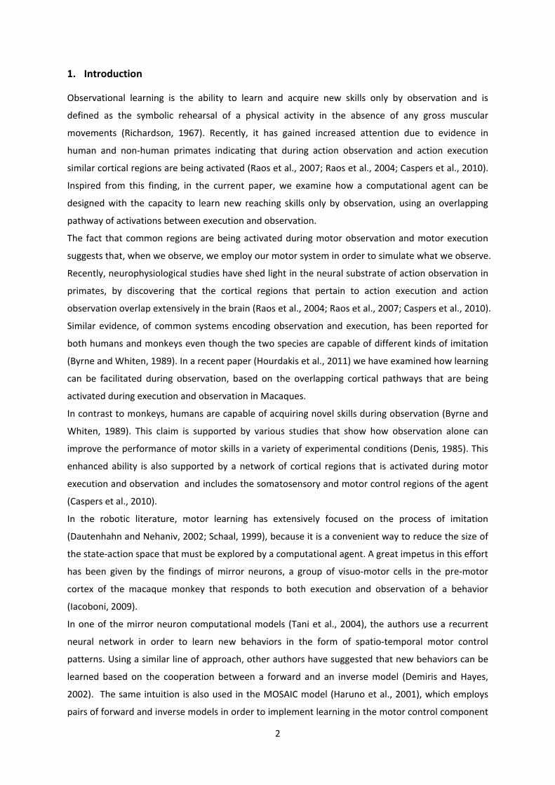
implementation based on liquid state machines (Fig. 6).

The complete architecture is shown in Fig. 6a, and consists of three neuronal components: (i) actors,

(ii) critics and (iii) liquid columns. In this architecture, the critic neurons are responsible for

predicting the rewards from the environment while the actor neurons for learning, using the

predicted reward signal, to activate the correct primitive based on the distance of the end-point

affector and the position of an object. For the current implementation, where a two-link planar arm

was used, this distance is defined in 2D coordinates. Figure 6b shows how these regions can be

mapped onto the model (Fig. 3, Reward circuit).

14

Fig. 6. a. The liquid state machine implementation of the actor-critic architecture. Each liquid column

is implemented using a liquid state machine with feedforward delayed synapses. The critics are

linear neurons, while the readouts are implemented using linear regression. b. The actor-critic

architecture mapped on the model of Fig. 3.

The input source to the circuit consists of Poisson spike neurons that fire at an increased firing rate

(above 80Hz) to indicate the presence of a certain event stimulus. Each input projects to a different

liquid column, i.e. a group of spiking neurons that is interconnected with feedforward, delayed,

dynamic synapses. The role of a liquid column is to transform the rate code from each input source

into a spatio-temporal pattern of action potentials in the spiking neuron circuitry (Fig. 7). The neuron

and synapse models used for the implementation of this circuit are described more thoroughly in

(Hourdakis and Trahanias, 2011). More specifically the synapses of the liquid were implemented as

simple analog synapses with delay, while the synapses for the critic and actor neurons were

implemented using the imminence weighting scheme. Transmission of the input spike signals is

carried out through the liquid columns, which consist of ten neuronal layers that each introduces a

delay of 5ms. This sort of connectivity facilitates the formation of a temporal representation of the

input, and implicitly models the timing of the stimulus events. The occurrence of an event results in

the activation of the first layer of neurons in a liquid column which is subsequently propagated

towards the higher layers with a small delay. This temporal representation is important for the

implementation of the imminence weighting scheme that is used to train the synapses of the

dopaminergic Critic neurons discussed below.

The Critic neurons (P1, P2, P3) model the dopamine neurons in the basal ganglia. Their role is to

learn to predict the reward that will be delivered to the agent in the near future. To accomplish this,

the critic neurons use the temporal representation that is encoded in each liquid column and

associate it with the occurrence of a reward from the environment. This is accomplished by training

the synapses between the liquid columns and the critic neurons in a way that they learn to predict

the occurrence of a reward by associating events in the near past.

15

Fig. 7. The spatio-temporal dynamics of an event as they are transformed by a liquid column. The

plot shows the temporal decay of a certain event by the liquid column’s output for four stereotypical

columns.

To implement the synapses between the liquid columns and the P, A neurons, we use the

imminence weighting scheme (Barto, 1994). In this setup, the critic must learn to predict the reward

of the environment using the weighted sum of past rewards: P = r + γr + γ r +⋯+ γ r (9)

where the factor γ represents the weight importance of predictions in the past and r is the reward

received from the environment at time t. To teach the critics to output the prediction of eq. (9) we

update their weights using gradient learning, by incorporating the prediction from the previous step: v = v + n[r + γP − P ]x (10) where v is the weight of the Critic at time t, n is the learning rate and x is the activation of the

critic at time t. The parameters γ, P and r are as in eq. (9). The weights of the actor are updated

according to prediction signal emitted by the critic:

v = v + n[r − P ]x (11) where v is the weight of the Actor at time t, n is the learning rate and x is the activation of the

actor at time t-1.

The basis of the imminence weighting scheme is that it uses the temporal representation of an input

stimulus, in order to learn to predict the forthcoming of a reward. Consequently, in the proposed

architecture, the actors, input the response of the neurons in the liquid state machine, and are

trained using the spatio-temporal dynamics of each liquid column (Fig. 7). The use of feed-forward

16

synapses within the liquid creates a temporal representation, i.e. activates different neurons, to

indicate the occurrence of a certain stimulus event at a specific time interval of the simulation. This

temporal representation is used by the imminence weighting scheme in order to learn to predict the

forthcoming of a reward.

The A1, A2, A3 neurons are trained using the signal emitted by the Critic neurons. To model them in

the current implementation we use a set of linear neurons. The input to each of these linear neurons

consists of a set of readouts that are trained to calculate the average firing rate of each liquid

column using linear regression. Each actor neuron is connected to all the readout units, with

synapses that are updated using gradient descent. In section 5 we illustrate how this circuitry can

replicate the properties of the dopaminergic neurons in the Basal Ganglia and help the agent learn

new behaviors by processing rewards.

4.3 Visual pathway

The role of the visual observation pathway (Fig. 3, Ventral visual stream) is to convert the iconic

representation of an object into a discrete class label. This label is used by the motor control and

planning pathways in order to associate the object with specific behavioral parameters. To

implement this circuitry, liquid state machines were also employed. To encode the input we first

sharpen each image using a Laplacian filter and consequently convolve it with 4 different Gabor

filters with orientations π, , 2π and − respectively.

The four convolved images from the input are projected into four neuronal grids of 25 neurons,

where each neuron corresponds to a different location in the Gabor output. The four

representations that are generated by the neuronal fields are injected into the liquid of an LSM

which creates a higher-order representation that combines the individual encoded output from each

Gabor image into an integrative representation in the liquid. Information from the liquid response is

classified using a linear regression readout that is trained to output a different class label based on

the object type.

In addition, the visual observation pathway (Fig. 3, Dorsal visual stream) includes a Liquid state

machine that is responsible for extracting basic parameters from the demonstrator’s movement. Its

input is modeled using a 25 neuronal grid which contains neurons that fire at an increased rate when

the position of the end-point effector of the demonstrator corresponds to the position defined in

the x, y coordinates of the grid. Information from this liquid is extracted using a readout that is

implemented as a feed-forward neural network, trained to extract the additional force that must be

applied by the higher-order control component in order to produce the demonstrated behavior. The

output of this readout is subsequently used in the higher-order control pathway during the

observational learning phase, in order to teach the model to produce the correct behavior.

17

4.4 State estimation pathway

The state estimation pathway consists of two components, a forward and an observation model. The

forward model is responsible for keeping track of the execution and imagined state estimates using

two different functions. To implement the first function we have designed the SI network to encode

the proprioceptive state of the agent using population codes (Fig. 3, SI), inspired from the local

receptive fields that exist in this region and the somatotopic organization of the SI.

To encode an end-point position we use a population code with 10 neurons for each dimension (i.e.

the x, y coordinates). Thus for the two dimensional space 20 input neurons are used. Neurons in

each population code are assigned a tuning value uniformly from the [0. .1] range. The input signal is

normalized to the same range. We then generate a random vectorv from a Gaussian distribution: v = G(100 − dev ∗ |I − T |, 2)(12) where I is the input signal normalized to the [0. .1] range, T is the neuron’s tuning value, and dev

controls the range of values that each neuron is selective to. The first part in the parenthesis of eq.

12 defines the mean of the Gaussian distribution. The second is the distribution’s variance.

Population codes assume a fixed tuning profile of the neuron, and therefore can provide a consistent

representation of the encoded variable. To learn the forward transformation we train a feedforward

neural network in the SPL region that learns to transform the state of the plant to a Cartesian x, y

coordinate (Fig. 3, Position hand-actor).

For the visual perception of the demonstrator’s movement we have also used a feedforward neural

network that inputs a noisy version (i.e. with added Gaussian white noise) of the perceived motion in

an allocentric frame of reference (Fig. 3, Position hand-observer). In this case the feedforward NN is

trained to transform this input into an egocentric frame of reference that represents the observed

state estimate of the agent, using backpropagation as the learning rule.

During observation, the role of the state estimation pathway is to translate the demonstrator’s

behavior into appropriate motoric representations to use in its own system. In the computational

modeling literature, this problem is known as the correspondence problem between one’s own and

others’ behaviors. To create a mapping between the demonstrator and the imitator we use

principles of self-organization, where homogenous patterns develop through competition into

forming topographic maps. This type of neural network is ideal for developing feature encoders,

because it forms clusters of neurons that respond to specific ranges of input stimuli.

The structure of the self-organizing map (SOM) is formed, through vector quantization, during the

execution phase based on the output of the forward model pathway discussed above. During its

training, the network’s input consists of the end point positions that have been estimated by the

forward model pathway, and its role is to translate them into discrete labels that identify different

position estimates of the agent (Fig. 3, Symbolic Component of movement).

18

The symbolic component is responsible for discretizing the output of the forward model pathway, so

that for different end-point positions of the robot’s hand, a different label will be enabled.

Fig. 8. A schematic illustration of the operation of the symbolic component. The end-point positions

of the agent’s different trajectories (marked in white circles in the left graph) are input into a self-

organizing map that quantifies the end point positions into labels that correspond to specific spaces.

The image shows one example in which a label from the self-organizing map (marked in red in the

grid of neurons on the right graph) corresponds to a specific space in the x, y Cartesian space in

which the agent’s hand moves.

During observation, the same network is input the transformed, in egocentric coordinates, state

estimate of the demonstrator’s movement, and outputs the respective labels that correspond to a

specific space in its x, y operating environment. In the results section we demonstrate how different

configurations of the SOM map affect the perception capabilities of our agent.

4.5 Reaching policy

Based on the higher order primitives and reward subsystems described above, the problem of

reaching can be solved by searching for a policy that will produce the appropriate joint torques to

reduce the error: q = q − q(13) where q is the desired state of the plant and q is its current state. In practice we do not know the

exact value of this error since the agent has only information regarding the end point position of its

hand and the trajectory that it must follow in Cartesian coordinates. However because our primitive

model is defined in Cartesian space, minimizing this error is equivalent to minimizing the distance of

the plant’s end point location with the nearest point in the trajectory: d = |l − t|(14) where and are the Cartesian coordinates of the hand and point in the trajectory, respectively. The

transformation from eq. (13) to eq. (14) is inherently encoded in the primitives discussed before. The

19

policy is learned based on two elements: (i) activate the correct combination of higher order

primitive force fields (Fig. 3, Motor control action), and (ii) set each one’s weight (Fig. 3, Hand/object

distance). The output of the actor neurons described in the previous section resembles the

activation of the canonical neurons in the premotor cortex (Rizzolatti and Fadiga, 1988), which are

responsible for gating the primitives. In a similar manner, every actor neuron in the reward

processing pathway is responsible for activating one of the primitives of the model, which in this

setup correspond to the up, down, left and right primitives. Due to the binary output of the actor

neurons, when a certain actor is not firing, its corresponding force field will not be activated. In

contrast, when an actor is firing, its associated force field is scaled using the output of the

hand/object distance component, mentioned above, and added to compose the final force.

To teach the actors the local control law, we use a square trajectory, which consists of eight

consecutive points p . . p . The model is trained based on this trajectory by starting from the final

location (p ) in four blocks. Each block contains the whole repertoire of movements up to that point.

Whenever it finishes a trial successfully, the synapses of each actor are changed based on a binary

reward, and training progresses to the next phase which includes the movement from the previous

block as well as a new one.

Reward is delivered only when all movements in a block have been executed successfully. Therefore,

the agent must learn to activate the correct force field primitives using the prediction signal from the

Critic neurons . The final torque that is applied on each joint is the linear summation of the scaled

primitives.

4.6 Higher-order control pathway

In the current paper, the higher-order control component is designed to inhibit the forces exerted by

the motor control component in a way that alters the curvature of approach towards the object (as

shown in Fig. 4B). This inhibition is realized as a force that is applied at the beginning of the

movement and allows the hand to approach the target object with different trajectories. To ensure

that the hand will reach the object in all cases, the effect of this force must converge to zero as the

hand approaches the target location. This allows the reaching component to progressively take over

the movement and ensure that the hand will arrive at the object. As shown in Fig. 4B, the magnitude

of the force is reduced (e.g. Fleft in Fig. 4B), and therefore the reaching force (RA) has a greater effect

on the movement.

To implement this concept computationally we use liquid state machines. The network consists of

two liquids of 125 neurons each, connected with the dynamic synapses and local connectivity (the

models of neurons and dynamic synapses that were used are the same as in the reward assignment

pathway). The first liquid is designed to model a dynamic continuous attractor which replicates the

decreasing aspects of the force, while the second is used to encode the values of the additional force

that will be exerted to the agent.

20

To replicate the decreasing aspect of the force on the attractor circuit we use a liquid that inputs two

sources; a continuous analog value and a discrete spike train. During training, the former, simulates

the dynamics of the attractor by encoding the expected rate as an analog value. The latter encodes

different starting values based on the perceived starting force of the demonstrator.

Fig. 9. The Liquid state machine circuit that implements the higher-order control component,

showing the two liquids and the input/readout neurons. The readout is trained to output the

decreasing force, i.e. which of the up, right, left and down primitives must be modulated in order to

change the strategy of approach towards an object. The attractor liquid implements an attractor

within the Liquid State Machine, based on the simulated input of the simulated attractor neuron.

The object label is input on the two liquids in order for the network to learn to associate an object

from the environment with its corresponding behavior.

The second liquid in the circuit consists of 125 neurons interconnected with local connectivity. The

input to the network consists of three sources. The first is the readout trained by the attractor circuit

that outputs the decreasing force. The second is the neuron that inputs the start force of the

movement. The third source is a population code that inputs the symbolic labels from the map of

the state estimation pathway. After collecting the states for the observer every 100ms, the liquid

states are trained for every label presented to the circuit up to that moment. The output of these

liquid states are trained using a feedforward neural network readout that must learn to approximate

the start force of the demonstrator and the decreasing rate of the force, based on the simulated

liquid states.

5. Results

In the current section we present experimental results that attest the effectiveness and

appropriateness of the proposed model. We first illustrate the training results for each individual

21

pathway of the model. We then continue to show the ability of the motor control component to

perform online reaching, i.e. reach towards any location with very little training. Finally, we present

the results of the observational learning process, i.e. the acquisition of new behaviors only by

observation.

5.1 Motor control component training

The first result we consider is the convergence of the least squares solution for the system of linear

equations in eq. (8). Figure 10 presents the solution for the “up” higher order primitive, where the

least squares algorithm has converged to an error value of 2, and created an accurate approximation

of the vector field. The three subplots at the bottom show three snapshots of the hand while moving

towards the “up” direction when this force field is active. Similar solutions were obtained for the

other three primitives, where the least squares solution converged to 7 (left), 2 (right) and 5 (down)

errors (the error represents the extent to which the directions of the forces in a field deviate from

the direction that is defined by the primitive).

Fig. 10. The force field (upper left subplot) and torque field (upper right subplot) as converged by the

least squares solution for the “up” primitive. The three subplots at the bottom show the snapshots

of the hand while moving when the primitive is active.

5.2 Reward assignment pathway

The policy for reaching was learned during an initial imitation phase where the agent performed the

training trajectory, and was delivered a binary reinforcement signal upon successful completion of a

whole trial. Since the reward signal was only delivered at the end of the trial, the agent relied on the

prediction of the reward signal elicited by the critic neurons. In the following we look more

22

thoroughly in the response properties of the simulated dopaminergic critic neurons and how the

actors learned to activate each force field accordingly based on this signal.

Figure 11a illustrates how the critic neurons of the model learned to predict the forthcoming of a

reward during training. In the first subplot (first successful trial) when reward is delivered at time

block 4, the prediction of the 1st critic is high, to indicate the presence of the reward at that time

step. After the first 10 successful trials (Fig. 11a, subplot 2), events that precede the presentation of

the reward (time block=3) start eliciting some small prediction signal. This effect is more evident in

the third and fourth subplots where the prediction signal is even higher at time block 3 and starts

responding at time block 2 as well. The effects of this association are more evident in Fig. 9b, where

it is shown how after training, even though rewards are not available in the environment, the

neurons start firing because they predict the presence of a reward in the subsequent steps. Using

the output of this prediction signal, the actor, i.e. in the case of the model the neurons that activate

the force fields in the motor control pathway, forms its weights in order to perform the required

reaching actions.

Fig. 11. a. An illustration of how the weights of one of the critic neurons from the reward processing

pathway are formed during the initial stages of the training (subplot 1), after Nt = 10 trials (subplot

2), after Nt = 20 trials (subplot 3) and after Nt = 30 trials (subplot 4). As the figure shows, the neuron

increases its output at time block 2 and 3, because it responds to events that precede the

presentation of a reward. b. The effect is evident in plot b, where the neuron learns to predict the

actual reward signal given to the robot at the end of a successful trial (upper subplot), by eliciting a

reward signal that predicts the presentation of the reward (bottom subplot). The x-axis represents

the 100ms time blocks of the simulation while the y-axis the values of the reward and prediction

signals respectively.

5.3 State estimation pathway

In the current section we present the results from the training of the two feedforward neural

networks that were used in order to implement the forward and observation models in the state

estimation pathway. In the first case, the network was trained in order to perform the forward

transformation from the proprioceptive state of the agent to the end point position of its hand. For

23

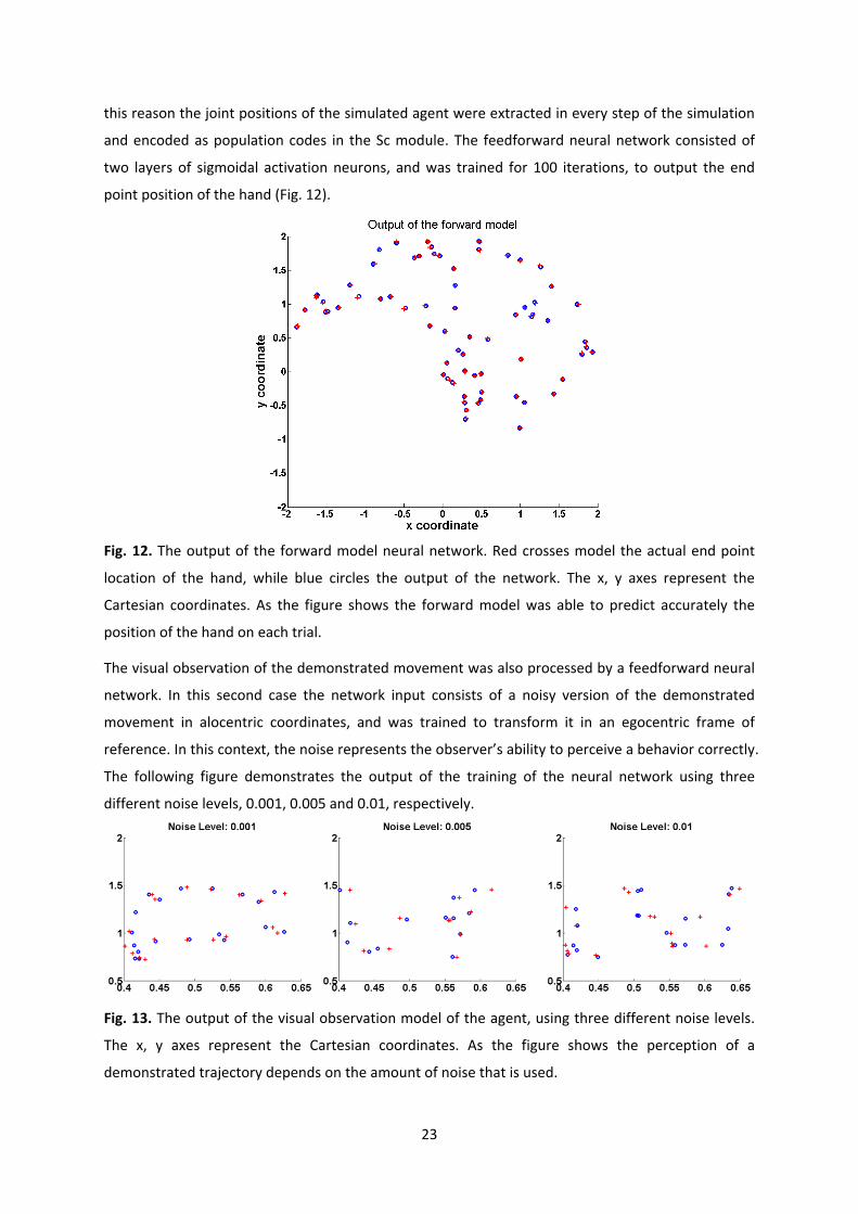
this reason the joint positions of the simulated agent were extracted in every step of the simulation

and encoded as population codes in the Sc module. The feedforward neural network consisted of

two layers of sigmoidal activation neurons, and was trained for 100 iterations, to output the end

point position of the hand (Fig. 12).

Fig. 12. The output of the forward model neural network. Red crosses model the actual end point

location of the hand, while blue circles the output of the network. The x, y axes represent the

Cartesian coordinates. As the figure shows the forward model was able to predict accurately the

position of the hand on each trial.

The visual observation of the demonstrated movement was also processed by a feedforward neural

network. In this second case the network input consists of a noisy version of the demonstrated

movement in alocentric coordinates, and was trained to transform it in an egocentric frame of

reference. In this context, the noise represents the observer’s ability to perceive a behavior correctly.

The following figure demonstrates the output of the training of the neural network using three

different noise levels, 0.001, 0.005 and 0.01, respectively.

Fig. 13. The output of the visual observation model of the agent, using three different noise levels.

The x, y axes represent the Cartesian coordinates. As the figure shows the perception of a

demonstrated trajectory depends on the amount of noise that is used.

24

In addition, the state estimation pathway included a self-organizing map whose role was to

discretize the end point positions of the observed or executed movements into symbolic labels. The

map was trained during the execution phase, where the agent was taught to perform elementary

reaching behaviors.

Fig. 14. Training of three SOM maps with different capacities for labels. In the first case the map

consisted of 25 labels, in the second of 81 labels and in the third of 144 labels. Red circles illustrate

the symbolic labels of the map, while black crosses the training positions of the agent’s movements.

Each map inputs the x, y coordinates of the agent’s movement, and outputs a symbolic label that

represents a specific space of the hand’s end point position (as shown in Fig. 8). A map with 144

labels (Fig. 14, 3rd subplot) can represent the output space of a behavior more accurately. All three

maps were evaluated during the observational learning stage against their ability to produce the

same labels during execution and observation.

5.4. Motor control – Hand/object distance component

To complete the implementation of the reaching policy the model must learn to derive the distance

of the end effector location from the current point in the trajectory. This is accomplished by

projecting the output from the forward model and the position of the object estimated by the visual

pathway in an LSM, and using a readout neuron to calculate their subtraction. In Fig. 15, we illustrate

two sample signals as input to the liquid (top subplot), the output of the readout neuron in the 10ms

resolution (middle subplot) and the averaged over the 100ms of simulation time output of the

readout neuron (bottom subplot).

25

Fig. 15. The output of the hand/object distance LSM after training. The top plot illustrates two

sample input signals of 5.5 seconds duration. The bottom two plots show the output of the neural

network readout used to learn the subtraction function from the liquid (middle plot), and how this

output is averaged using a 100ms window (bottom plot). From the 3rd subplot it is evident that the

LSM can learn to calculate with high accuracy the distance between the end-point position of the

hand and position of the target object.

5.5 Online reaching

Having established that the individual pathways/components of the proposed model operate

successfully, we now turn our attention to the performance of the model in various reaching tasks.

The results presented here are produced by employing the motor control, reward assignment and

state estimation pathways only. We note here that the model wasn’t trained to perform any of the

given reaching tasks, apart from the initial training/imitation period at the beginning of the

experiments. After this stage the model was only given a set of points in a trajectory and followed

them with very good performance.

To evaluate the performance of the model we used two complex trajectories. The first required the

robot to reach towards various random locations spread in the robot’s workspace (Fig. 16a,

Trajectory 1) while the second complex trajectory required the robot to perform a circular motion in

a cone shaped trajectory (Fig. 16a, Trajectory 2). Figure 16a illustrates how the aforementioned

trajectories were followed by the robot.

To evaluate the model performance quantitatively we created 100 random trajectories and tested

whether the agent was able to follow them. Each of these random movements was generated by

first creating a straight line trajectory (Fig. 16b, left plot) and then randomizing the location of 2, 3 or

4 of its points; an example is illustrated in Fig. 16b, right plot.

26

Fig. 16. a. Two complex trajectories shown to the robot (red points) and the trajectories produced by

the robot (blue points). Numbers mark the sequence with which the points were presented. b. The

template used to generate the random test set of 100 trajectories (left plot) and a random trajectory

generated from this template (right plot).

The error was calculated by summing the overall deviation of the agent’s movement from the points

in the trajectory for all the entries in the dataset. The results indicate that the agent was able to

follow all trajectories with an average error of 2%. This suggests that the motor control component

can confront, with high accuracy, any reaching task.

5.6 Planning circuit and attractor tuning

As mentioned in section 4, the higher-order control circuit consists of 2 liquids which model the

decreasing force that is exerted to the hand of the agent. Herewith we present the results of the

attractor liquid. As Fig. 17 illustrates, the readout unit can produce a stable response despite the

varying liquid dynamics. The output of the readout is used to inhibit directly the force produced by

the motor control component. As the figure shows, the attractor dynamics cause the output of the

readout to descent to zero after the first steps of the simulation.

Fig. 17. The output of the trained readout that models the force exerted by the higher-order control

pathway (bottom subplot, blue line) and the desired force value (bottom subplot, red line) for the

same period. The top subplot illustrates the input to the circuit. The x axis in all plots represents time

in 100ms intervals.

27

5.7 Observational learning

In this section we illustrate the results from the observational learning experiments, which involve

the function of all the pathways of the model. To test the ability of the agent to learn during

observation we have generated sample trajectories by simulating the model using predefined

parameters. The agent was demonstrated one trajectory at a time, and its individual pathways were

trained for 1500ms. The same simulation time was used during the execution of the respective

motor control behaviors, i.e. 1500ms. Training of the model in this phase regarded only to the

convergence of the higher-order control pathway, and consequently it only required a few number

of trials (40 trials for the results shown in Figs 18, 19) for the model to converge to a solution. The

role of this phase was to evaluate the agent’s ability to learn a demonstrated trajectory only by

observation, i.e. without being allowed to move its hand. Subsequently, to evaluate the extent to

which the agent learned the demonstrated movement we run an execution trial, where the agent

was required to replicate the demonstrated behavior.

Figure 18 illustrates a sample trajectory that was demonstrated to the agent (left, red circles), the

output of the planning module (Fig. 18, bottom right), the corresponding class labels generated by

the model, and the state of the agent during observation for a 1500ms trial (Fig. 18, top right). The

noise used for the visual observation pathway was 0.05 while the size of the state estimation map

was 81 labels. The optimal result that should be accomplished, which is the trajectory demonstrated

to the robot, is shown in red circles.

Fig. 18. The observed state of the hand during observational learning. The left subplot illustrates the

trajectory demonstrated (red circles) and the trajectory perceived by the agent (blue squares). The

top right subplot illustrates the output of the SOM in the state estimation pathway, while the

bottom right subplot illustrates the output of the linear regression readout in the planning pathway

(red circles are the desired values of the force, blue boxes are the output of the readout).

28

As the figure illustrates (Fig. 18, left subplot) the agent was able to keep track of the demonstrated

trajectory with very good accuracy. The top right subplot in Fig. 18 illustrates the class labels that

were generated by the state estimation pathway using the visual observation pathway’s output in

green and the states (in red) that would have been generated if the agent was executing the

behavior covertly. In blue we mark the labels generated during the first errorenous trial. As the top-

right subplot illustrates the model was able to match the perceived trajectory (green line) with the

one it should execute (red line) with high accuracy. This improvement was accomplished after 100

learning trials during which the sum of squares error of the deviation of each trajectory, reduced

from 9 units to 0.2 units. To verify that the agent learned the new behavior after the observational

learning phase we run the same simulation using the forward model for the state estimation. The

following figure illustrates the trajectory that was actually executed by the agent during execution

(Fig. 19). The optimal result that should be accomplished, which is the trajectory demonstrated to

the robot, is shown in red circles.

Fig. 19. The trajectory executed by the robot during the execution phase. The left subplot illustrates

the trajectory demonstrated (red circles) and the trajectory executed by the agent (blue squares).

As discussed in section 4, the noise levels and size of the state estimation map had a direct effect on

the performance of the model. Larger noise levels altered the perception of the agent and

compromised its ability to mentally keep track of the observed movement. The following figure

illustrates the response of the agent for 0.01, 0.05, 0.1 and 0.3 noise levels respectively.

Fig. 20. The executed trajectory under the impact of noise. The four subplots show the trajectory

executed by the agent with different values of noise.

29

As the results of this section demonstrate the developed computational agent is able to acquire new

motor skills only by observation. The quality of learning is correlated with the agent’s perceptual

abilities, i.e. the extent to which it can perceive an observed action correctly. This skill is facilitated

due to the design of the model that allows new motor skills to be learned based on a set of simple

parameters that can be derived only by observation.

6. Discussion

In the current paper we presented a computational implementation of observational learning. We

have exploited the fact that when observing, humans activate the same pathway of regions as when

executing. The cognitive interpretation of this fact is that when we observe, we use our motor

system, i.e. our own grounded motor experiences, in order to understand what we observe. The

developed model was able to learn new motor skills only by observation, by adopting the peripheral,

higher-order control component of its motor system during observation.

The fact that the brain activates the same pathways to simulate an observed action is an important

component of human intelligence, and as it has been suggested (Baron-Cohen et al., 1993), a basis

for social cognition. In the computational modeling community, most research in this area has

focused on the function of mirror neurons. The evidence of activating pathways throughout the

cerebral cortex suggests that the cortical overlap of the regions is much more extended than the

mirror neuron mechanism. More importantly, since action observation activates the same regions as

in action execution, observational learning can be used to revise our understanding about the

content of motor representations. Computational models, such as the one presented, may

potentially facilitate our understanding regarding the basis under which all these processes operate

together in order to accomplish a behavioral task.

To evaluate the model’s ability to learn during observation we have employed a two-link simulated

planar arm, with simplified simulation conditions. To compensate for the uncertainty in the

measurements of a real world environment we have incorporated noise within the perceptual

streams of the agent. This simplified condition is enough to prove our assumption, that learning can

be implemented during observation using the simulation of the motor control system, however in

order to transfer the model into a real-world embodiment one must take under consideration

additional issues, regarding the encoding of the proprioceptive information of the agent and the

visual streams. In the future, we plan to extend the model in order to compensate for these issues,

by looking into the function and structure of the proprioceptive association and visual estimation

model pathways.

The model was designed to perform two main functions: (i) online reaching, i.e. enable the agent to

reach towards any given location with very little training, and (ii) observational learning, i.e. the

acquisition of novel skills only by observation. To implement the reaching component we have

devised a local reaching policy, where the computational model exerts forces that move the hand

30

towards a desired location. The benefit of this approach is that any errors in the movement can be

compensated at the later stages of motor control. Learning during observation was implemented on

the higher-order control component based on simple parameters. This intuition was very important

for the implementation of the observational learning process, since the agent wasn’t required to

restructure its whole motor system in order to acquire new behaviors. In the current

implementation, during the execution of a reaching trajectory we used only the proprioceptive

feedback of the agent in order to guide the movement. In real-world conditions, primates also have

access to additional visual information derived from the perception of their hand. Due to the fact

that the addition of such component can provide benefits into producing more stable movements, in

the future we plan to consider how this visual feedback can be integrated within the suggested

model.

Having established a working model of observational learning, one of the important aspects that we

plan to investigate in the future is the cortical underpinnings of motor inhibition during observation.

More specifically, what are the reasons that cause the human’s body to stay immobile during

observation. Cortically, inhibition must exist at the spinal levels by preventing the excitation of the

muscle reflexes (Baldissera et al., 2001). For this reason, we plan to exploit possible implementations

of the cerebellum, and how its function can allow us to inhibit specific components of the movement.

Moreover, we also plan to focus on implementing agency attribution, i.e. the process that allows the

cortical agents to perceive their body as their own. Both processes are considered very important to

observational learning and their implementation may significantly contribute towards our

understanding of relevant biological mechanisms.

Acknowledgements

The work presented in this paper has been partly supported by the European Commission funded

project MATHESIS, under contract IST-027574.

The authors would also like to thank the anonymous reviewers for their valuable comments and

suggestions that helped improve the quality of the manuscript.

31

References

Baldissera F, Cavallari P, Craighero L, FadigaL. (2001). Modulation of spinal excitability during

observation of hand actions in humans. Eur. J. Neurosci. v.13:1, pp.90–94.

Barto, A.G. (1994). Adaptive critics and the basal ganglia, Models of information processing in the

basal ganglia, MIT Press, Cambridge.

Bentivegna D. C. and Atkeson C. G. (2002). Learning how to behave from observing others. In Proc.

SAB'02- Workshop on Motor Control in Humans and Robots:on the interplay of real brains and

artificial devices, Edinburgh, UK, August, 2002.

Billard, A., & Hayes, G. (1999). DRAMA, a connectionist architecture for control and learning in

autonomous robots. Adaptive Behavior, v.7:1, pp.35–63.

Bizzi E., Mussa-Ivaldi F.A., and Giszter S.F., (1991). Computations Underlying the Execution of

Movement: A Novel Biological Perspective. Science, v. 253, pp.287–291.

Byrne, R. and Whiten, A. (1989). Machiavellian Intelligence: Social Expertise and the Evolution of

Intellect in Monkeys, Apes, and Humans, Oxford Science Publications, Oxford.

Caspers, S. and Zilles, K. and Laird, A.R. and Eickhoff, S.B. (2010). ALE meta-analysis of action

observation and imitation in the human brain. Neuroimage, v.50, pp. 1148-1167.

Corke P.I. (1996) A Robotics Toolbox for MATLAB, IEEE Robotics and Automation Magazine, v.1,

pp.24-32

Chaminade, T. and Meltzoff, A.N. and Decety, J. (2005). An fMRI study of imitation: action

representation and body schema, v.43:1, pp.115-127.

Dautenhahn, K. and Nehaniv C.K., (2002). Imitation in animals and artifacts. Cambridge MA: MIT

Press.

Decety, J., Philippon, B. and Ingvar, D.H. (1988). rCBF landscapes during motor performance and

motor ideation of a graphic gesture. Eur. Arch. Psychiatry Neurol. Sci., v.238, pp.33-38.

Decety, J. and Ryding, E. and Stenberg, G. and Ingvar, D.H. (1990). The cerebellum participates in

mental activity: tomographic measurements of regional cerebral blood flow. Brain Research,

v.535:2, pp.313-317.

Decety, J., Perani, D., Jeannerod, M., Bettinardi, V., Tadary, B., Woods, R., Mazziotta, J.C. and Fazio, F.

(1994). Mapping motor representations with PET. Nature, v.371, pp.600-602.

Degallier, S. and Ijspeert, A., (2010). Modeling discrete and rhythmic movements through motor

primitives: a review, Biological Cybernetics, v.103:4, pp.319-338.

Demiris, Y., & Hayes, G. (2002). Imitation as a dual-route process featuring predictive and learning

components: A biologically-plausible computational model. In K. Dautenhahn, & C. Nehaniv

(Eds.), Imitation in animals and artifacts. Cambridge, MA: MIT Press.

Demiris Y and Simmons G,. 2006, Perceiving the unusual: Temporal properties of hierarchical motor

representations for action perception, Neural Networks, v.19:3, pp. 272-284

32

Denis, M. (1985). Visual imagery and the use of mental practice in the development of motor skills.

Canad. J. Applied Sport Sci., v.10 pp.4-16

Elshaw, M., Weber, C., Zochios, A., & Wermter, S. (2004). An associator network approach to robot

learning by imitation through vision, motor control and language. International joint conference

on neural networks, Budapest, Hungary.

Fabbri-Destro, M. and Rizzolatti, G., (2008). Mirror neurons and mirror systems in monkeys and

humans. Physiology 23, 171–179.

Fieldman, J.B., Cohen, L.G., Jezzard, et al. (1993). Functional neuroimaging with echo-planar imaging

in humans during execution and mental rehearsal of a simple motor task. 12th Annual Meeting of

the Society of Magnetic Resonance in Medicine, pp. 1416.

Finke, R.A. (1980). Levels of equivalence in imagery and perception. Psychol. Rev., v.87 pp.113-132.

Gallese, V. and Fadiga, L. and Fogassi, L. and Rizzolatti, G. (1996). Action recognition in the premotor

cortex. Brain, v. 119: pp.593-609.

Georgopoulos, A., Kalaska, J., Caminiti, R. & Massey, J. (1982). On the relations between the

direction of two-dimensional arm movements and cell discharge in primate motor cortex. J.

Neurosci. v.2, pp.1527–1537.

Giszter, S.F, Mussa-Ivaldi, F.A. and Bizzi, E. (1993). Convergent force fields organized in the frog’s

spinal cord, Journal of Neuroscience, v.13:2, pp.467.

Haruno, M., Wolpert, D. M., & Kawato, M. (2001). Mosaic model for sensorimotor learning and

control. Neural Computation, v.13:10, pp.2201–2220.

Heuer, H.A, (1989). Multiple-representations’ approach to mental practice of motor skills, in: B.

Kirkcaldy (Ed). Normalities and Abnormalities in Human movement, v.29, pp.36–57, Med Sport

Science, Basel, Karger.

Hourdakis E. and Trahanias P. (2011). Computational modeling of online reaching, European

Conference on Artificial Life, ECAL11, Paris, France.

Hourdakis Ε., Savaki Ε. and Trahanias P. (2011). Computational modeling of cortical pathways

involved in action execution and action observation, Neurocomputing, v. 74:7, pp.1135-1155.

Hourdakis E. and Trahanias P. (2011). Observational learning based on overlapping pathways, Second

International Conference on Morphological Computation, MORPHCOMP11, Venice, Italy.

Iacoboni, M. (2009). Imitation, empathy, and mirror neurons. Annu. Rev. Psychol. v.60, pp.653–670.

Jeannerod, M., (1994). The representing Brain: Neural correlates of motor imagery and intention.

Behav. Brain Sci., v.17, pp.187-245.

Kaas, J.H., R.J. Nelson, M. Sur, C.S. Lin, and M. M. Merzenich. (1979). Multiple representations of the

body within the primary somatosensory cortex of primates. Science, v.204:4392, pp.521-523.

Maass, W. and Natschlaeger, T. and Markram, H. (2002). Real-time computing without stable states:

A new framework for neural computation based on perturbations, Neural Computation, v.14:11,

pp. 2531-2560.

33

Oztop, E. & Arbib, M. A. (2002). Schema design and implementation of the grasp-related mirror

neuron system. Biol. Cybern. v.87, pp.116–140.

Parsons LM, Gabrieli JDE, Phelps EA, Gazzaniga MS., (1998). Cerebrally lateralized mental

representations of hand shape and movement. J Neurosci, v.18, pp.6539-6548.

Perani, D. and Fazio, F. and Borghese, N.A. and Tettamanti, M. and Ferrari, S. and Decety, J. and

Gilardi, M.C. (2001). Different brain correlates for watching real and virtual hand actions, v.14:3,

pp.749-758.

Raos, V. and Evangeliou, M.N. and Savaki, H.E. (2004). Observation of action: grasping with the

mind's hand, Neuroimage, v.23:1, pp.193-201, Elsevier.

Raos, V. and Evangeliou, M.N. and Savaki, H.E. (2007). Mental simulation of action in the service of

action perception, v.27:46, pp.12675--12683.

Richardson, A. (1967). Mental practice: A review and discussion, Part 1. Research Quarterly, v.38,

pp.95-107.

Rizzolatti G. and Fadiga L. (1998). Grasping objects and grasping action meanings: the dual role of

monkey rostroventral premotor cortex (area F5). Wiley.

Rizzolatti, G., (2005). The mirror neuron system and its function in humans. Anat. Embryol. v.210,

pp.419–421.

Roland, P.E., Skinhoj, E., Lassen, N.A. and Larsen, B., (1980). Different cortical areas in man in

organization of voluntary movements in extrapersonal space. J. Neurophysiol., v.43, pp.137-150.

Sackett, R. S. (1935). The relationship between amount of symbolic rehearsal and retention of a

maze habit. Journal of General Psychology, v.13, pp.113-128.

Saunders, J. and Nehaniv, C.L. and Dautenhahn, K. (2004). An experimental comparison of imitation

paradigms used in social robotics, Robot and Human Interactive Communication, 2004. ROMAN

2004. 13th IEEE International Workshop on, pp. 691-696

Savaki E. (2010). How do we understand the actions of others? By mental simulation not mirroring,

Cognitive Critique, v.2, p.99-140.

Saxe, R., S. Carey, and Kanwisher N., (2004). Understanding other minds: Linking developmental

psychology and functional neuroimaging. Ann. Rev. Psychol., v.55, pp.87-124.

Scassellati. B. (1999). Imitation and mechanisms of joint attention: A developmental structure for

building social skills. In C. L. Nehaniv, editor, Computation for Metaphors, Analogy and Agents,

v.1562, pp.176-195. Springer Lecture Notes in Artificial Intelligence,

Schaal, S. (1999). Is imitation learning the route to humanoid robots? Trends Cogn. Sci. v.3, pp.233–

242.

Schaal, S. and Ijspeert, A. and Billard, A. (2003) Computational approaches to motor learning by

imitation, Philosophical Transactions of the Royal Society of London. Series B: Biological Sciences,

v.358:1431, pp.537-547.

34

Schultz, W. and Tremblay, L. and Hollerman, J.R. (2000). Reward processing in primate orbitofrontal

cortex and basal ganglia, Cerebral Cortex, v.10:3, pp.272.

Schwartz, A. B. (1994). Direct cortical representation of drawing. Science, v.265, pp.540–542.

Tani, J., Ito, M., & Sugita, Y. (2004). Self-organization of distributed represented multiple behavior

schemata in a mirror system: Reviews of robot experiments using RNNPB. Neural Networks,

v.17:8–9, pp.1273–1289.

Touwen, B. C. L. (1998). The brain and development of function. Developmental Review. v.18:4,

pp.504-526.

title: computational modeling of observational learning

Documents