Some thoughts on regression modeling forobservational and longitudinal data

W. John Boscardin

October 16, 2018

Outline

I Choosing predictors for a regression model

I Missing data

I Repeated/longitudinal measurements

Recurring Theme

I ”Essentially all models are wrong, but some are useful”(George E. P. Box)

I I would add that whichever wrong model you end up using inyour analysis, there are many others that you could have used– your model is not particularly special and you should takecare not to overinterpret it.

Building a regression model

I Harrell, Lee, Mark (1996)

I Sullivan, Massaro, D’Agostino (2004)

I Steyerberg et al. (2010)

Typical Setting for Model Building

I Long-term survival data on adults age 70+ (n ≈ 1000, e.g.).

I Have maybe P = 50 baseline, admission, dischargecharacteristics potentially predicting survival

I Goal: build a reasonably parsimonious (p = 10 or p = 15predictors), clinically practical and sensible model that hasgood discrimination and calibration

I Move from statistical model to something simple and clinicallyuseful (make easy to calculate 5 year survival probabilities ormedian life expectancy for given individual)

Statistical models for risk prediction

I Logistic regression (or other binary regression)

I Cox regression (or other time-to-event models)

I Multinomial regression (for multi-state outcomes)

Predictions

I Key idea: don’t just look at (odds/hazard) ratios for thepredictors

I Instead focus on predicted probabilities from the fitted models

I For logistic regression get predicted probability of event forgiven characteristics

I For Cox regression, same but at specific time points

Choosing predictors

I Many possibilities all with pros and cons; combinableFrankenstein’s monster-style

I Theoretical guidance/DAGI Existing risk model or index (incremental value of your shiny

new predictor)I Practicality/Simplicity/Cost of obtaining predictorsI Bivariate screeningI Forward/Backward/Stepwise selectionI ”Best” subset methods

Automatic subset selection

I Many sources have criticized stepwise model selection:I Standard errors of coefficients artificially smallI Coefficient estimates biased away from zeroI R2 biased upwardI Performs poorly in presence of multicollinearity

I Best subset selection usually viewed as even worse in all ofthese senses than stepwise

I Ronan Conroy: “I would no more let an automatic routineselect my model than I would let some best-fit procedure packmy suitcase”.

A Slightly Different View

I All of these things true (to some extent), but I think there ismore important point

I Stepwise selection only shows one model and does not outputcomparisons to other potential models

I Best subsets regression gives a huge amount of usefulinformation for comparing models, and in practice, a largenumber of models of reasonable parsimony are statisticallynearly indistinguishable

I It is tremendously valuable to clinicians to view a lot ofsimilarly performing prognostic models to choose ones thatare most practically applied

I All the other criticisms can be addressed with bootstrapping

Best Subsets Selection

I Computationally infeasible to fit all 2P possible subset models

I But for each of p = 1, 2, 3, ...,P − 1 it is blazingly fast (usingboth branch and bound and properties of score test) to findthe best (or best k) models according to score statistic(similar to log-likelihood)

I This gives a list of k(P − 1) models most of which are good insome sense

I Typical finding (Miao et al., 2014) is that dozens of modelswill all have same c-statistic and may be quite different ininterpretation/simplicity/etc.

Best Subsets 1

Best Subsets 2

Best Subsets 3

Assessing fit: discrimination

I Discrimination demonstrations:I C-statistic for binary regressionI Harrell’s c-statistic for time-to-event modelsI Ad hoc variants on c-statistic for multi-state outcome models

(e.g. collapse outcomes into dichotomous versions and usebinary regression methods)

I Graphically/Tabularly want to show large differences inpredicted outcomes

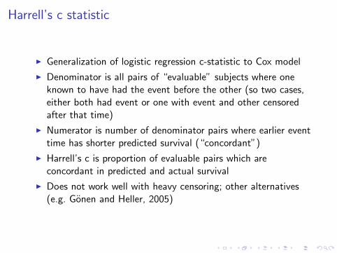
Harrell’s c statistic

I Generalization of logistic regression c-statistic to Cox model

I Denominator is all pairs of “evaluable” subjects where oneknown to have had the event before the other (so two cases,either both had event or one with event and other censoredafter that time)

I Numerator is number of denominator pairs where earlier eventtime has shorter predicted survival (“concordant”)

I Harrell’s c is proportion of evaluable pairs which areconcordant in predicted and actual survival

I Does not work well with heavy censoring; other alternatives(e.g. Gonen and Heller, 2005)

Incremental value

I Typically improvement in c-statistic very small with your shinynew predictor (e.g. c=0.83 new model vs. c=0.82 old model)

I Sometimes reclassification indices provide better insight intoincremental value (NRI and IDI)

Assessing fit: calibration

I Calibration demonstrations:I Binary regression: show that predicted event rates and

observed event rates match up (graphically use calibrationplot, numerically use Hosmer-Lemeshow test maybe)

I Time-to-event models: look at fixed time points (e.g. 5 yearsurvival) and use binary regression methods

I Multi-state models: show that predicted event rates andobserved event rates match up

Calibration plot (Steyerberg, 2010)

Table Format (Mehta, 2011)

Discrimination Plot (Steyerberg, 2010)

Simplex discrimination (Barnes, 2013)

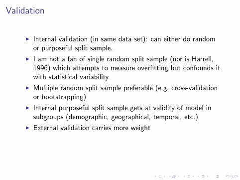
Validation

I Internal validation (in same data set): can either do randomor purposeful split sample.

I I am not a fan of single random split sample (nor is Harrell,1996) which attempts to measure overfitting but confounds itwith statistical variability

I Multiple random split sample preferable (e.g. cross-validationor bootstrapping)

I Internal purposeful split sample gets at validity of model insubgroups (demographic, geographical, temporal, etc.)

I External validation carries more weight

Overfitting

I “Over-optimism” has two components

I 1. whatever procedure was used to select a good model wasalmost certainly driven by data at hand

I 2. the coefficients for that model are optimized to provide thebest fit to the data at hand

I When assessing the model performance in a new data set, wewill almost always have degradation in the model performancemeasure

I With a single split sample, you can’t separate randomvariability from systematic overfitting

I Can address with repeated split sampling (e.g. cross-validationor bootstrapping)

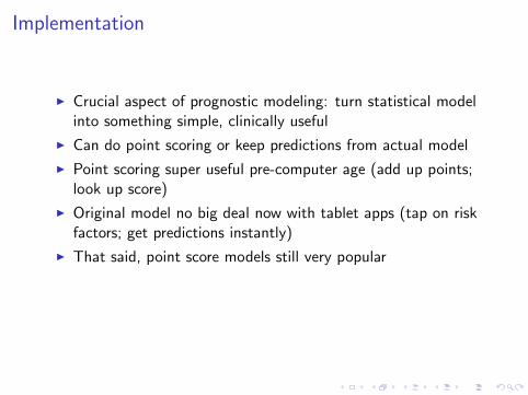
Implementation

I Crucial aspect of prognostic modeling: turn statistical modelinto something simple, clinically useful

I Can do point scoring or keep predictions from actual model

I Point scoring super useful pre-computer age (add up points;look up score)

I Original model no big deal now with tablet apps (tap on riskfactors; get predictions instantly)

I That said, point score models still very popular

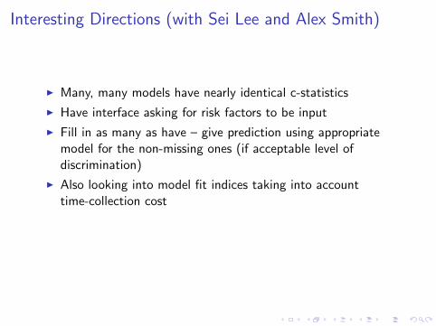
Interesting Directions (with Sei Lee and Alex Smith)

I Many, many models have nearly identical c-statistics

I Have interface asking for risk factors to be input

I Fill in as many as have – give prediction using appropriatemodel for the non-missing ones (if acceptable level ofdiscrimination)

I Also looking into model fit indices taking into accounttime-collection cost

Handling Missing Data

I White, Royston, Wood (2011)

I Royston (2004)

I Little and Rubin (2002)

Common Setting for Missing Data

I Have a large number of potential predictors in a regressionanalysis

I Regression software will drop cases that have any missing data

I Many of the predictors are missing in the data set

I Even if small percentage of missing for any particular predictormight have only a handful of subjects with no missing data forany predictors

Imputation of Missing Data

I Various procedures to fill in the missing data so that thesesubjects are not dropped from the analysis have been used forpast 40 years

I Suppose want to regress blood pressure on weight, height,gender, etc, but that some weights are missing in the data set

I One idea is to fill in the mean weight for all missing weights

I Slightly better idea is to fill in the mean weight for all thosewith same height and gender

Multiple Imputation

I Problem is that the fill-in is uncertain.

I Key idea: fill in a random draw from the set of all weights ofthose with same height and gender and do so a number (M)of times. This is called Multiple Imputation (MI)

I Can then do the regression in each of these M complete datasets

I Combine the M sets of regression coefficients using Rubin’srules (Little and Rubin, 2002; Carlin et al., 2008)

Rubin’s Rules

I Estimate of a parameter is the average of the parameterestimates from each imputed data set

I Standard error of a parameter combines the within imputationSE and between imputation SD

MI in software and in practice

I Twenty years ago, MI was a nice idea in theory

I Now MI is easily available in SAS, Stata, and R, for example

I First widely available algorithm was NORM (Schafer, 1997).Assumes multivariate normal distribution for all quantities ofinterest. Variants allow some relaxation of this. Backbone ofProc MI in SAS

I Specially modified version of NORM used to do the officialmultiple imputations for NHANES III (Schafer et al., 1996);other government data have official MIs (e.g. Schenker et al.,2006)

NHANES III imputation

(from the official documentation of NHANES III-MI“NH3MI.DOC”)

One key feature of the imputation models is that they are based

upon an assumption of multivariate nomality; that is, they assume

that the variables to be imputed are (individually and jointly)

normally distributed within demographic subgroups defined by age,

sex, and race/ethnicity. Some variables that consist of discrete

categories (e.g. self-reported health status, which takes values

from 1 = excellent to 5 = poor) were modeled and imputed as if they

were normally distributed, and the continuous imputed values were

rounded off to the nearest category. Other variables whose

distributions were skewed were transformed by standard power

functions such as the logarithm, square root, or reciprocal square

root; modeling and imputation were carried out on the transformed

data, and after imputation they were transformed back to the

original scale....

Simple example in NHANES

. mi set mlong

. mi register imputed kstones sbp dbp male age smoke maxwt

. mi misstable patterns, frequency

Missing-value patterns

(1 means complete)

| Pattern

Frequency | 1 2 3 4 5

------------+------------------

17,751 | 1 1 1 1 1

|

954 | 1 1 1 0 0

618 | 1 1 0 1 1

464 | 1 0 1 1 1

62 | 1 0 1 0 0

57 | 1 1 0 0 0

42 | 0 1 0 1 1

29 | 1 0 0 1 1

22 | 0 1 0 0 0

11 | 1 0 0 0 0

8 | 0 1 1 1 1

6 | 0 0 0 0 0

3 | 0 0 0 1 1

2 | 0 1 1 0 0

------------+------------------

20,029 |

Variables are (1) smoke (2) maxwt (3) age (4) dbp (5) sbp

Complete cases regression

Lose almost 12% of the data set.

logistic kstones sbp dbp male age smoke maxwt

Logistic regression Number of obs = 17751

LR chi2(6) = 346.65

Prob > chi2 = 0.0000

Log likelihood = -3170.0128 Pseudo R2 = 0.0518

------------------------------------------------------------------------------

kstones | Odds Ratio Std. Err. z P>|z| [95\% Conf. Interval]

-------------+----------------------------------------------------------------

sbp | .9998493 .0020883 -0.07 0.942 .9957646 1.003951

dbp | 1.008443 .0031585 2.68 0.007 1.002272 1.014653

male | 1.474334 .1137626 5.03 0.000 1.267405 1.715048

age | 1.028355 .0023434 12.27 0.000 1.023773 1.032959

smoke | .8614465 .069716 -1.84 0.065 .7350916 1.009521

maxwt | 1.005423 .0008747 6.22 0.000 1.00371 1.007139

------------------------------------------------------------------------------

Imputing data

mi impute chained (regress) sbp (regress) dbp (logit) male (regress)

age (logit) smoke (regress) maxwt, add(10)

note: variable male contains no soft missing (.) values; imputing nothing

Conditional models:

smoke: logit smoke i.male maxwt age sbp dbp

maxwt: regress maxwt i.male i.smoke age sbp dbp

age: regress age i.male i.smoke maxwt sbp dbp

sbp: regress sbp i.male i.smoke maxwt age dbp

dbp: regress dbp i.male i.smoke maxwt age sbp

Performing chained iterations ...

Multivariate imputation Imputations = 10

Chained equations added = 10

Imputed: m=1 through m=10 updated = 0

Initialization: monotone Iterations = 100

burn-in = 10

MI Logistic Regression (MC error)

. mi estimate, mcerror: logistic kstones sbp dbp male age smoke maxwt

Logistic regression Number of obs = 20029

Largest FMI = 0.1300

------------------------------------------------------------------------------

kstones | Coef. Std. Err. t P>|t| [95\% Conf. Interval]

-------------+----------------------------------------------------------------

sbp | .0013643 .0020714 0.66 0.510 -.0027044 .005433

| .0002225 .0000516 0.10 0.066 .0002038 .0002842

|

dbp | .0059833 .0030078 1.99 0.047 .0000822 .0118843

| .0002665 .0000477 0.08 0.009 .0002537 .0003112

|

male | .4154024 .0730054 5.69 0.000 .2723141 .5584907

| .0012741 .0000642 0.02 0.000 .0012587 .0013017

|

age | .0270061 .0022828 11.83 0.000 .0225226 .0314895

| .0002419 .0000342 0.20 0.000 .0002485 .0002558

|

smoke | -.1498978 .0771103 -1.94 0.052 -.301032 .0012364

| .0018016 .0001164 0.02 0.003 .0017323 .0018961

|

maxwt | .0050521 .0008346 6.05 0.000 .0034163 .0066878

| .0000302 2.72e-06 0.04 0.000 .0000302 .0000311

|

_cons | -6.207185 .2778718 -22.34 0.000 -6.752047 -5.662324

| .0200949 .0046794 0.43 0.000 .0157049 .0271742

------------------------------------------------------------------------------

Note: values displayed beneath estimates are Monte Carlo error estimates.

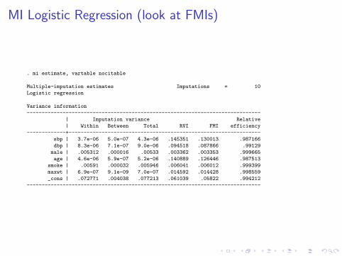
MI Logistic Regression (look at FMIs)

. mi estimate, vartable nocitable

Multiple-imputation estimates Imputations = 10

Logistic regression

Variance information

------------------------------------------------------------------------------

| Imputation variance Relative

| Within Between Total RVI FMI efficiency

-------------+----------------------------------------------------------------

sbp | 3.7e-06 5.0e-07 4.3e-06 .145351 .130013 .987166

dbp | 8.3e-06 7.1e-07 9.0e-06 .094518 .087866 .99129

male | .005312 .000016 .00533 .003362 .003353 .999665

age | 4.6e-06 5.9e-07 5.2e-06 .140889 .126446 .987513

smoke | .00591 .000032 .005946 .006041 .006012 .999399

maxwt | 6.9e-07 9.1e-09 7.0e-07 .014592 .014428 .998559

_cons | .072771 .004038 .077213 .061039 .05822 .994212

------------------------------------------------------------------------------

Alphabet Soup

I Missing completely at random (MCAR): probability of missingdoes not depend on observed or on missing data(e.g. recording instrument fails 10% of the time)

I Missing at random (MAR): probability of missing dependsonly on observed data (e.g. men who smoke more likely to bemissing blood pressure)

I Missing not at random (MNAR): missingness probabilitydepends on missing values (e.g. when maximum weight wasvery high more likely not to report it)

Assumptions and Methods

I Dropping subjects with any missing data (listwise deletion)may lead to biased estimates of parameters (unless MCAR)and always leads to inefficient estimates

I Multiple imputation routines can give unbiased estimates ofparameters of interest assuming data are MAR and will almostalways be more efficient

I Practical advice: if include everything remotely relevant inchained equations then MAR is much more plausible (similarto propensity score idea)

I If MNAR, need to run more advanced models as sensitivitycheck (Daniels and Hogan, 2008)

And Now for Something Completely Different

I Recent problem reflecting real-world complexity!

I VA data on providers (approximately 10K providers)

I About 15% missing provider genderI Several potential strategies:

I Gender from name algorithms (e.g. genderize.io) withexternal databases

I Same algorithms but in internal databaseI Impute using multiple imputation from provider specialty,

patient mix demographics, etcI Assign some by expert judgement!

I Optimal combination of strategies is not trivial

Summary

I Switching regressions (SR) is incredibly intuitive and flexiblemethod for generating multiple imputations

I SR is still on somewhat shaky theoretical ground statistically,but a number of recent papers (e.g. Lee and Carlin, 2010)have shown it works quite well

I SR is now seamlessly integrated into Stata (mi impute

chained) as of Version 12

I Stata multiple imputation works with nearly every regressionroutine and also handles survey weights!

Repeated Measures and Longitudinal Data

I Repeated or longitudinal measurements on subjects verycommon in studies

I Can be very useful to address confounding but also addscomplexity to modeling

I Will discuss some commonly used models

Mixed Effects Regression Models

I Make model for average trajectory in time

I Assume each patient has their own patient-specific trajectorycentered around the average trajectory

I Many parametric choices for shape of trajectory (e.g. linear,polynomial, spline)

I Can also use non-parametric shapes via penalized orsmoothing splines

Average Shape Remarks

I Might focus on average trajectory. The mixed model used toproperly account for intra-patient correlation of longitudinaldata

I Buries under rug the likely inter-patient heterogeneity aroundthese average trajectories

I Two components of heterogeneity: (i) noisiness of individualdata; (ii) variation of shape in individual trajectories

Subject-Specific Trajectories

I Goal: estimate subject-specific linear trajectories.I Can use these estimated trajectories for variety of purposes:

I Direct statistically valid inference on subject-specific timetrajectories

I Classify subjects according to characteristics of subject-specifictime trajectories (e.g. increasers vs. decreasers, slow vs. quickincreasers)

I Inference on time to threshold crossing

I More reliant on model being correct

Random Slopes and Intercepts Example

10

20

30

40

50

60

70

50 100 150

28 9

50 100 150

5 40

50 100 150

6 43

50 100 150

27 4

50 100 150

22 38

50 100 150

2

49 25 55 10 16 12 42 56 24 52

10

20

30

40

50

60

70

20

10

20

30

40

50

60

70

13

50 100 150

1 14

50 100 150

54 53

50 100 150

8 31

50 100 150

21 23

50 100 150

41 18

SPHR

CS

FL

AC

CSFlac vs. Post-Injury Hour (93 studies on 33 patients)

Cubic Splines Average Trajectory

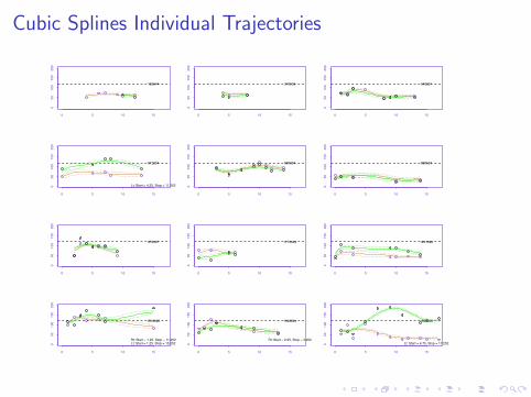
Cubic Splines Individual Trajectories

0 5 10 15

05

01

00

15

02

00

163644

0 5 10 15

05

01

00

15

02

00

376538

0 5 10 15

05

01

00

15

02

00

540091

0 5 10 15

05

01

00

15

02

00

812254

Lt: Start = 4.25, Stop = 11.252

0 5 10 15

05

01

00

15

02

00

890004

0 5 10 15

05

01

00

15

02

00

890524

0 5 10 15

05

01

00

15

02

00

979467

0 5 10 15

05

01

00

15

02

00

1172329

0 5 10 15

05

01

00

15

02

00

1241380

0 5 10 15

05

01

00

15

02

00

1516060

Rt: Start = 1.25, Stop = 11.252Lt: Start = 1.25, Stop = 15.252

0 5 10 15

05

01

00

15

02

00

1548864

Rt: Start = 2.25, Stop = 3.252

0 5 10 15

05

01

00

15

02

00

1548866

Lt: Start = 4.75, Stop = 17.252

Cubic Spline Trajectory Example

Logarithmic Recovery Example

Discrete Timepoints

I Most longitudinal cohort studies have only a small number oftimepoints that are common to all subjects (e.g. at baselineand at every 2 years after baseline)

I Rather than looking at baseline as time 0 can look atpost-enrollment event-of-interest times (which are oftenobtained continuously) as time 0

I Example: physical functioning before and after hospitalization

I For an event that happens at roughly constant rate,timepoints will be roughly uniformly distributed

HRS Data Setting

I Nationally representative study of older Americans.

I Bigger sample size but fewer timepoints (less frequent) thanBrown

I Total of 7000 subjects, 5000 hospitalized during study (andsmaller subgroups are of interest)

I Have 5 measurement occasions per subject (every 2 yearsvs. every 6 months in Brown)

I How good of a job can we do estimating Brown model with2-3 before and 2-3 after?

I How can we argue that we have enough power to look atquestions of interest!

Simulated Data

I Use fitted model from Brown to simulate data

I Use sample size and time point frequency from my datasource of interest

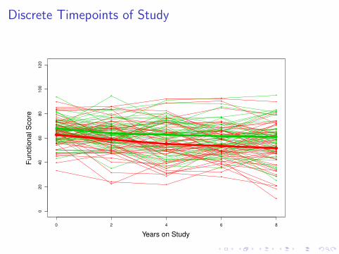
Discrete Timepoints of Study

0 2 4 6 8

020

40

60

80

100

120

Years on Study

Fu

nctio

na

l S

co

re

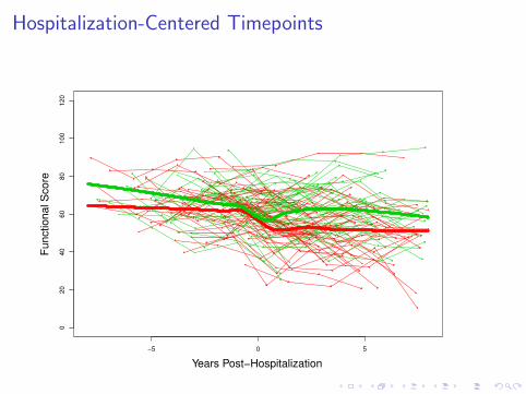
Hospitalization-Centered Timepoints

−5 0 5

020

40

60

80

100

120

Years Post−Hospitalization

Fu

nctio

na

l S

co

re

Four parameter model (Single group)

I tij = Time since hospitalization for subject i , occasionj = 1, 2, 3, 4, 5

I hij = Indicator of post-hospitalization time, i.e. hij ≡ 1tij>0

I rij = Logarithmic time post-hospitalization,i.e. rij ≡ log(hij tij + 1)

I β1 = Intercept (average score at t = 0)

I β2 = Pre-hospitalization slope

I β3 = Amount score drops at time of hospitalization

I β4 = Recovery slope on logarithmic time scale

Logarithmic recovery model

−4 −2 0 2 4

35

40

45

50

55

60

65

70

Years Post−Hospitalization

Fu

nctio

na

l S

co

re

β1

β3

Slope β2

Slope (log) β4

Two group logarithmic recovery model

−4 −2 0 2 4

35

40

45

50

55

60

65

70

Years Post−Hospitalization

Fu

nctio

na

l S

co

re

A few more modeling details

I Random effects for intercept and drop at time ofhospitalization in what I will discuss here

I Have binary covariate indicating type of hospitalization(surgical vs. non-surgical) distributed roughly 50/50

I Add interactions of intercept, slope, drop, recovery with thecovariate

Fitted Model

−5 0 5

020

40

60

80

100

120

Years Post−Hospitalization

Fu

nctio

na

l S

co

re

General remarks

I A sample size of 5000 subjects with a 50/50 split of thehospitalization-type covariate is enough to get extremelyprecise estimates of the parameters in the Brown et al. model

I Acceptable precision (i.e. enough power to discern clinicallymeaningful differences)

Latent Trajectory Models

I Assume there are a small number (k) of discrete categories ofpatients

I Category is unknown (latent) for each patient

I Simultaneously estimate the latent class memberships (get aprobability for each patient belonging to each class) and the ktrajectories

I Has become very popular method in past several years largelydue to SAS Traj procedure (Jones et al., 2001) and recentNEJM article (Gill et al., 2010)

Latent Trajectory Example 1

Latent Trajectory Discussion

I Visually can be powerful way to display heterogeneity in data

I However, estimated latent trajectories may not be clinicallydistinct

I Statistically “optimal” solution masks near-optimality of manyquite different solutions

I Look at Bandeen-Roche plots (next slide) for visual check onmodel fit

Latent Trajectory Example 1

Latent Trajectory vs. Mixed Effects

I As mentioned can also use mixed effects to categorize patientsinto small number of groups based on the subject-specifictrajectories

I This is fairly common application in practice

I Ignores uncertainty in group membership, however

I Latent class makes this explicit by reporting probabilities ofgroup membership

I Can get group membership probabilities for mixed effectsapproach using Bayesian inference (now available in procsmixed/mcmc)

References

I Barnes DE, Mehta KM, Boscardin WJ, Fortinsky RH, Palmer RM, Kirby KA,Landefeld CS (2013). A prognostic index to predict recovery, dependence, ordeath in elders who become disabled during hospitalization. J Gen Intern Med,28:261-268.

I Harrell FE, Lee KL, Mark DB (1996). Tutorial in Biostatistics: Multivariableprognostic models. Stat Med, 15, 361–387.

I King (2003). Running a best-subsets logistic regression: an alternative tostepwise methods. Educ Psych Meas, 63, 392–403.

I Mehta KM, Pierluissi E, Boscardin WJ, Kirby K, Walter L, Chren M, Palmer R,Counsell S, Landefeld CS (2011). A clinical index to stratify hospitalized olderpatients according to risk for new-onset disability. J Am Geriatr Soc,59:1206-1216.

I Miao Y, Cenzer I, Kirby K, Boscardin WJ. (2013) Estimating Harrell?sOptimism on Predictive Indices Using Bootstrap Samples Proc SAS GlobalForum, 2013:504.

I Steyerberg EW, Vickers AJ, Cook NR, Gerds T, Gonen M, Obuchowski N,Pencina MJ, Kattan MW (2010). Assessing the performance of predictionmodels: a framework for traditional and novel measures. Epidem, 21, 128–138.

I Sullivan LM, Massaro JM, D’Agostino RB (2004), Presentation of multivariatedata for clinical use: The Framingham Study risk score functions. Stat Med,23,1631?1660.

References (2)

I Carlin JB, Galati JC, Royston P (2008). A new framework for managing andanalyzing multiply imputed data in Stata. Stata Journal 8, 49–67.

I Daniels MJ, Hogan JW (2008). Missing data in longitudinal studies: strategiesfor Bayesian modeling and sensitivity analysis. New York: CRC.

I Jones B, Nagin D, Roeder K (2001). A SAS procedure based on mixture modelsfor estimating developmental trajectories. Sociol Method Res, 29, 374–393.

I Lee KJ and Carlin JB (2010). Multiple imputation for missing data: Fullyconditional specification versus multivariate normal imputation. Am J of Epid,171, 624–632.

I Li, K.-H. 1988. Imputation using Markov chains. J Stat Comp Simulation.

I Little RJA and Rubin DB (2002). Statistical analysis with missing data, 2nded.. New York: Wiley.

I Raghunathan TE, Lepkowski JM, Van Hoewyk J, Solenberger P (2001). Asequential regression imputation for survey data. Survey Methodology, 27,85–96.

I Royston P (2004). Multiple imputation of missing values: update. StataJournal, 5, 188–201.

References (3)

I Rubin, DB (1976). Inference and Missing Data. Biometrika, 63, 581–592.

I Schafer, JL (1997). Analysis of incomplete multivariate data. New York: CRC.

I Schafer JL, Ezzatti-Rice TM, Johnson W, Khare M, Little RJA, Rubin, DB(1996). The NHANES III multiple imputation project. ASA Proc of SurveyResearch Methods Section, 28–37.

I Schenker N, Raghunathan TE, Chiu PL, Makuc DM, Zhang GY, Cohen AJ(2006). Multiple imputation of missing income data in the National HealthInterview Survey. J Am Stat Assoc, 101, 924–933.

I van Buuren S, Boshuizen HC, Knook DL (1999). Multiple imputation of missingblood pressure covariates in survival analysis. Stat Med, 18, 681–694.

I van Buuren S, Brand JPL, Groothuis-Oudshoorn K, Rubin DB (2006). Fullyconditional specification in multivariate imputation. J Stat Comp Sim, 76,1049–1064.

I van Buuren S (2007). Multiple imputation of discrete and continuous data byfully conditional specification. Stat Meth Med Res, 16, 219–242.

I White IR, Royston P, Wood AM (2011). Multiple imputation using chainedequations: Issues and guidance for practice. Stat Med, 30, 377-99.