lecture 22 - university of waterlooleung.uwaterloo.ca/mns/102/lect_2013/lect_22b.pdf · lecture 22...

Lecture 22 MNS 102: Techniques for Materials and Nano Sciences

• X-ray diffraction (XRD)

• Rontgen and X-ray generation

• Laue, Laue equations, and diffraction

• Braggs, and Bragg’s Law

• Single-crystal and four-circle XRD

• Powder XRD

• Bragg-Brentano parafocussing setups

• Diffraction from a single crystal and from a polycrystal

• Information obtained by XRD

• Phase ID, quantitative analysis, crystallinity and stress, texture and orientation, crystallite size

• Limitations of XRD

1 22-

Reference: #1 C. R. Brundle, C. A. Evans, S. Wilson, "Encyclopedia of Materials Characterization", Butterworth-Heinemann, Toronto (1992), Ch. 4.1 Reference: #4 W. D. Callister, "Materials Science and Engineering: An Introduction", 7th ed., Wiley, New York (2006), Ch. 3, 12, 14. - Also other editions.

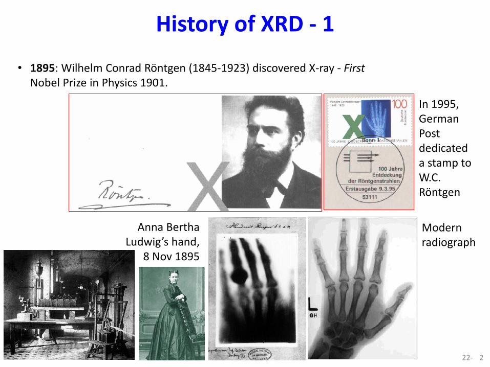
History of XRD - 1

• 1895: Wilhelm Conrad Röntgen (1845-1923) discovered X-ray - First Nobel Prize in Physics 1901.

22- 2

In 1995, German Post dedicated a stamp to W.C. Röntgen

Anna Bertha Ludwig’s hand,

8 Nov 1895

Modern radiograph

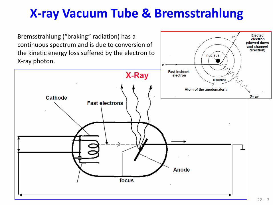
X-ray Vacuum Tube & Bremsstrahlung

22- 3

Bremsstrahlung (“braking” radiation) has a continuous spectrum and is due to conversion of the kinetic energy loss suffered by the electron to X-ray photon.

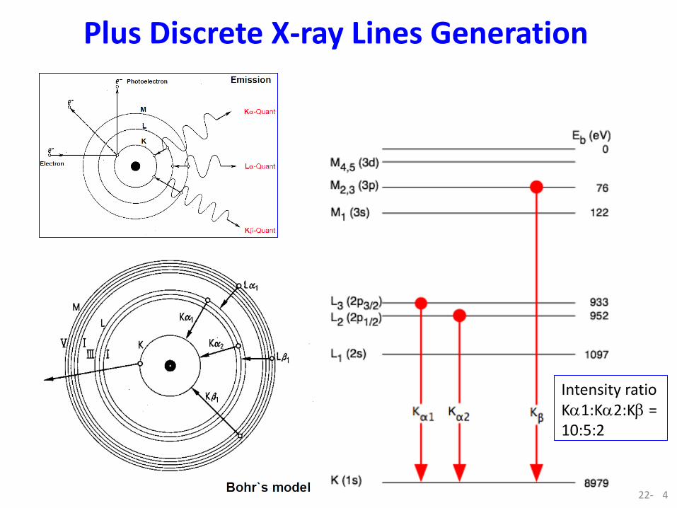
Plus Discrete X-ray Lines Generation

22- 4

Intensity ratio K1:K2:K = 10:5:2

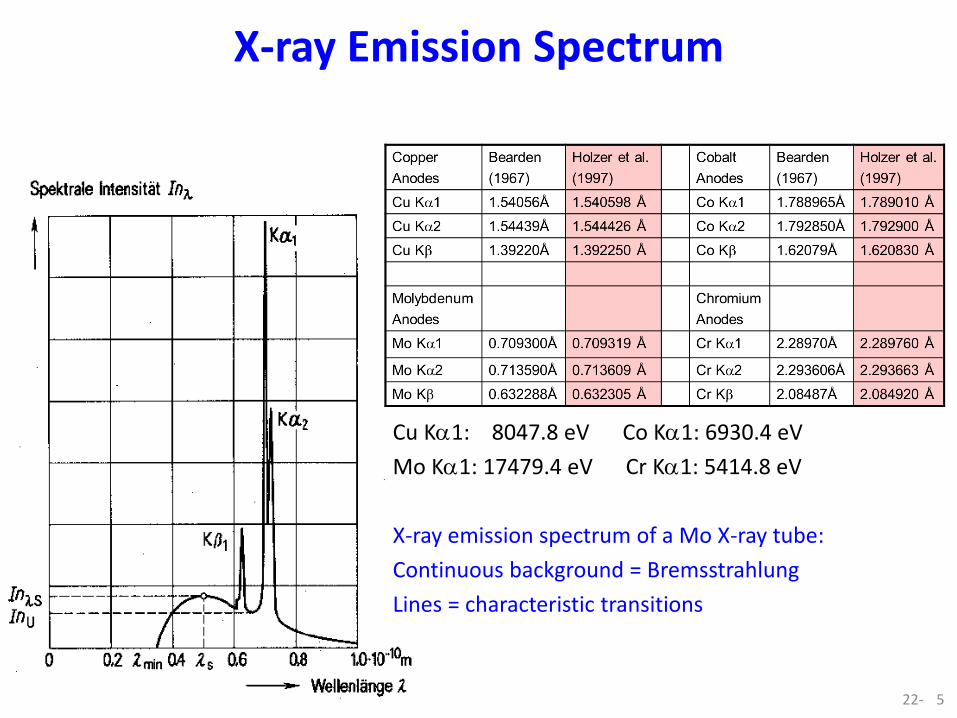
X-ray Emission Spectrum

22- 5

Cu K1: 8047.8 eV Co K1: 6930.4 eV

Mo K1: 17479.4 eV Cr K1: 5414.8 eV

X-ray emission spectrum of a Mo X-ray tube:

Continuous background = Bremsstrahlung

Lines = characteristic transitions

Modern X-ray Tube

X-ray source: Cu Kα: 1.54Å ; Mo Kα: 0.71Å Safety: 1 Sievert (Sv) = Exposing to X-ray source running at 45 kV 30 mA for 1 min 1 Sv = 100 REM; 1 mSv = 0.1 mREM • Hair loss 1-3 Sv, blisters 5-12 Sv; • Natural Background Radiation = 3 mSv/yr; • Chest X-ray = 2.4 day NBR = 0.02 mSv; • Computed Tomography diagnostic scan =

1-10 mSv; • Japanese survivors of atomic bombs =

2-20 mSv; • Flight from Toronto to Vancouver ~

0.03 mSv; • Radon gas at our home ~ 2 mSv/yr.

22- 6

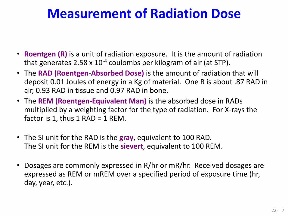
Measurement of Radiation Dose

• Roentgen (R) is a unit of radiation exposure. It is the amount of radiation that generates 2.58 x 10-4 coulombs per kilogram of air (at STP).

• The RAD (Roentgen-Absorbed Dose) is the amount of radiation that will deposit 0.01 Joules of energy in a Kg of material. One R is about .87 RAD in air, 0.93 RAD in tissue and 0.97 RAD in bone.

• The REM (Roentgen-Equivalent Man) is the absorbed dose in RADs multiplied by a weighting factor for the type of radiation. For X-rays the factor is 1, thus 1 RAD = 1 REM.

• The SI unit for the RAD is the gray, equivalent to 100 RAD. The SI unit for the REM is the sievert, equivalent to 100 REM.

• Dosages are commonly expressed in R/hr or mR/hr. Received dosages are expressed as REM or mREM over a specified period of exposure time (hr, day, year, etc.).

22- 7

History of XRD - 2

• 1912: Max Theordor Felix von Laue (1879-1960) (U of Munich) thought that X-ray has a wavelength similar to interatomic distances in crystals and the crystal should act like a 3D diffraction grating. Along with Walter Friedrich (research assistant) and Paul Knipping (PhD grad student), he did the first diffraction experiment on CuSO4 crystal – Nobel Prize in Physics 1914.

22- 8

9

Physics of Diffraction

• Diffraction = apparent bending of waves around small obstacles or spreading of wave past small openings ~ interference.

• Diffraction gratings must have spacings comparable to the wavelength of diffracted radiation. See: http://www.youtube.com/watch?v=-mNQW5OShMA

• Cannot resolve interplanar spacings that are less than .

22-

Source: http://en.wikipedia.org/wiki/Diffraction

http://www.youtube.com/watch?v=-mNQW5OShMA



http://en.wikipedia.org/wiki/Diffraction

http://en.wikipedia.org/wiki/Diffraction

X-ray interactions with a Crystal

• Like any electromagnetic radiation, X Rays are diffracted, reflected, scattered incoherently, absorbed, refracted, and transmitted when they interact with matter.

• Diffraction occurs when each object in a periodic array scatters radiation coherently, producing concerted constructive interference at specific angles.

• The electrons in an atom coherently scatter light b/c the electrons interact with the oscillating electric field of the light wave.

• Atoms in a crystal form a periodic array of coherent scatterers.

– The wavelength of X rays are similar to the distance between atoms.

– Diffraction from different planes of atoms produces a diffraction pattern, which contains information about the atomic arrangement within the crystal.

22- 10

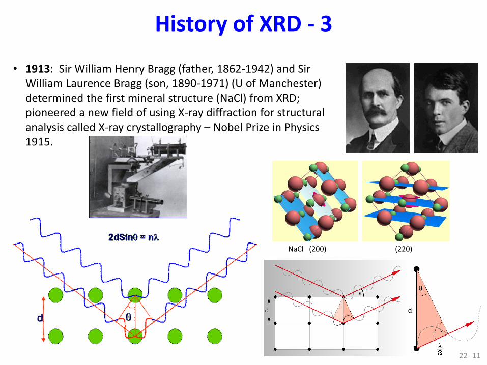
History of XRD - 3

• 1913: Sir William Henry Bragg (father, 1862-1942) and Sir William Laurence Bragg (son, 1890-1971) (U of Manchester) determined the first mineral structure (NaCl) from XRD; pioneered a new field of using X-ray diffraction for structural analysis called X-ray crystallography – Nobel Prize in Physics 1915.

22- 11

NaCl (200) (220)

12

Bragg’s Law

Detected X-ray

intensity

q q c

d = n 2 sin q c

Measurement of critical angle, qc, allows computation of interplanar spacing, d.

• Incoming X-rays diffract from the crystal planes. For constructive interference, the path length difference (PLD) must be integral wavelengths, i.e. PLD = 2 (d sin q) = n

• Once we know d, then we can work out the lattice parameters, 1/d2hkl = h2/a2 + k2/b2 + l2/c2

e.g. For cubic lattices (a = b = c), 1/d2hkl = (h2 + k2 + l2) /a2

Adapted from Fig. 3.19, Callister 7e.

reflections must be in phase for a detectable signal

Spacing between planes

d

q

q extra distance or path length difference travelled by wave “2”

22-

13

XRD Pattern

Source: Callister 5e.

(110)

(200)

(211)

z

x

y a b

c

Diffraction angle 2q

Inte

nsity (

rela

tive

)

z

x

y a b

c

z

x

y a b

c

22-

Two Types of XRD Instruments: 1. Single-crystal or Four-circle XRD (sometimes known as high-resolution XRD) – great for thin films and materials characterization; and 2. Powder XRD – Primary for materials science.

Single-crystal XRD

22- 14

Single-Crystal (Laue) Diffraction – a beam of X-rays of “all” wavelengths is directed at a single crystal, which sits stationary in front of a photographic plate. A series of diffraction spots surround the central point of the beam, corresponding to diffraction from a given series of atomic planes.

Four-circle XRD

22- 15

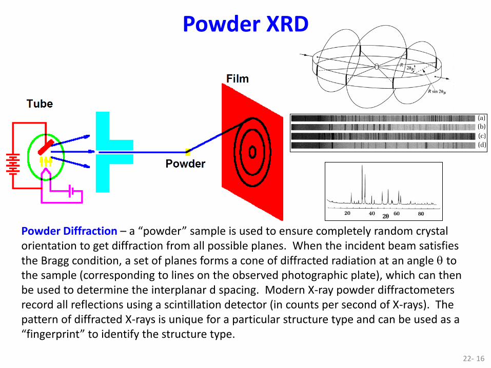
Powder Diffraction – a “powder” sample is used to ensure completely random crystal orientation to get diffraction from all possible planes. When the incident beam satisfies the Bragg condition, a set of planes forms a cone of diffracted radiation at an angle q to the sample (corresponding to lines on the observed photographic plate), which can then be used to determine the interplanar d spacing. Modern X-ray powder diffractometers record all reflections using a scintillation detector (in counts per second of X-rays). The pattern of diffracted X-rays is unique for a particular structure type and can be used as a “fingerprint” to identify the structure type.

22- 16

Powder XRD

WATLab PANalytical X’Pert Pro MRD

22- 17

Powder Diffraction – a “powder” sample is used to ensure completely random crystal orientation to get diffraction from all possible planes. When the incident beam satisfies the Bragg condition, a set of planes forms a cone of diffracted radiation at an angle q to the sample (corresponding to lines on the observed photographic plate), which can then be used to determine the interplanar d spacing. Modern X-ray powder diffractometers record all reflections using a scintillation detector (in counts per second of X-rays). The pattern of diffracted X-rays is unique for a particular structure type and can be used as a “fingerprint” to identify the structure type.

22- 18

Powder XRD

Powder XRD

22- 19

Bragg Brentano parafocussing – Theta-2Theta: X-ray tube is stationary, move sample by theta and simultaneously move detector by 2theta (Rigaku RU300) or Theta-theta: Sample is stationary, move X-ray tube and detector simultaneously by theta (PANalytical X’Pert Pro MPD)

WATLab PANalytical X’Pert Pro MPD

22- 20

A single-crystal specimen in a Bragg-Brentano diffractometer would produce only one family of peaks in the diffraction pattern.

At 20.6 °2q, Bragg’s law fulfilled for the (100) planes, producing a diffraction peak.

The (110) planes would diffract at 29.3°2q but they are not properly aligned to produce a diffraction peak (the perpendicular to those planes does not bisect the incident and diffracted beams). Only background is observed.

The (200) planes are parallel to the (100) planes. They also diffract for this crystal. Since d200 is ½ d100, they appear at 42°2q.

2q

Source: http://prism.mit.edu/xray 22- 21

A polycrystalline sample should contain thousands of crystallites. All possible diffraction peaks should therefore be observed.

• For every set of planes, there will be a small percentage of crystallites that are properly oriented to diffract (the plane perpendicular bisects the incident and diffracted beams).

• Basic assumptions of powder diffraction are that for every set of planes there is an equal number of crystallites that will diffract and that there is a statistically relevant number of crystallites, not just one or two.

2q 2q 2q


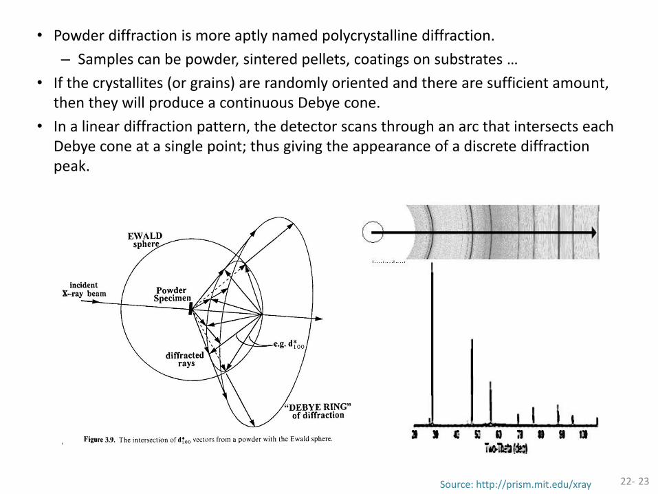
• Powder diffraction is more aptly named polycrystalline diffraction.

– Samples can be powder, sintered pellets, coatings on substrates …

• If the crystallites (or grains) are randomly oriented and there are sufficient amount, then they will produce a continuous Debye cone.

• In a linear diffraction pattern, the detector scans through an arc that intersects each Debye cone at a single point; thus giving the appearance of a discrete diffraction peak.


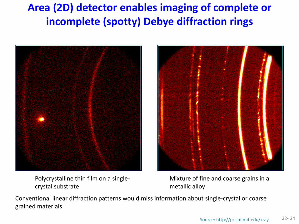
Area (2D) detector enables imaging of complete or incomplete (spotty) Debye diffraction rings

Polycrystalline thin film on a single-crystal substrate

Mixture of fine and coarse grains in a metallic alloy

Conventional linear diffraction patterns would miss information about single-crystal or coarse grained materials


Information obtained by XRD

22- 25

• Phase Composition of a Sample – Quantitative Phase Analysis: determine the relative amounts of phases in a mixture

by referencing the relative peak intensities (relative areas under the peaks). • Unit cell lattice parameters and Bravais lattice symmetry

– Index peak positions; use ICDD PDF (Powder Diffraction File) database to ID over 760,000 diffraction patterns (ICDD = International Centre for Diffraction Data http://www.icdd.com/ ).

– Lattice parameters could change as a function of different growth and/or processing conditions, and depend on alloying, doping, solid solutions, strains, etc.

• Crystal Structure – By Rietveld refinement (least-squares minimization) of the entire diffraction pattern.

• Residual Strain (macrostrain) • Epitaxy/Texture/Orientation (texture = distribution of orientations) • Crystallite Size, and Defects

– Indicated by peak broadening, use Scherrer equation. – Other defects (stacking faults, etc.) can be measured by analysis of peak shapes and

peak width. • In-situ processing – Depending on the diffractometer… Some can be used to characterize

the above as a function of time, temperature, and gas environment.

q

=q

cosW

K2D

where D is crystallite size, W is the FWHM, and K= 0.94

http://www.icdd.com/


22- 26

Information Content

Diffraction Intensities

• The integrated intensity (peak area) of each powder diffraction peak is given by the following expression:

I(hkl) = |S(hkl)|2 × Mhkl × LP(θ) × TF(θ)

– S(hkl) = Structure Factor

– Mhkl = Multiplicity

– LP(θ) = Lorentz & Polarization Factors

– TF(θ) = Temperature Factor (more correctly referred to as the displacement parameter)

The above does not include effects that can sometimes be problematic such as absorption, preferred orientation and extinction.

• The structure factor reflects the interference between atoms in the basis (within the unit cell). All of the information regarding where the atoms are located in the unit cell is contained in the structure factor. The structure factor is given by the following summation over all atoms (from 1 to j) in the unit cell:

S(hkl) = Σj fj exp {-i2π(hxj+kyj+lzj)}

– fj = form factor for the j-th atom

– h, k & l = Miller indices of the hkl reflection

– xj, yj & zj = The fractional coordinates of the jth atom

22- 27

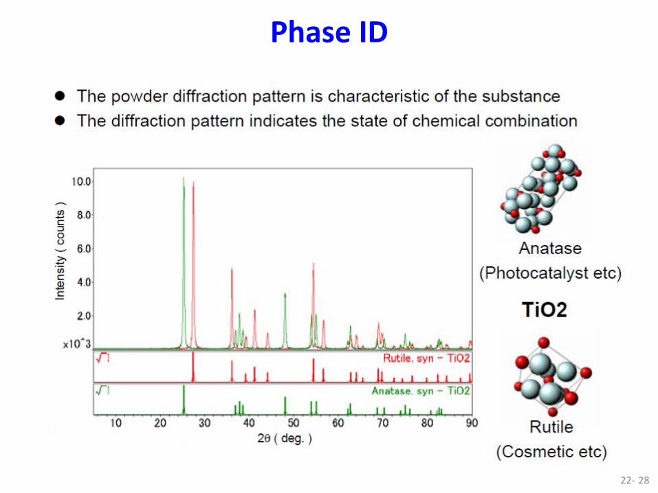
Phase ID

22- 28

22- 29

ICDD Powder Diffraction File (PDF) Card

22- 30 International Centre for Diffraction Data http://www.icdd.com/


22- 31

PDF#46-1212: QM=Star(S); d=Diffractometer; I=Diffractometer Corundum, syn Al2 O3 Radiation=CuKa1 Lambda=1.540562 Filter= Calibration= 2T=25.578-88.994 I/Ic(RIR)= Ref: Huang, T., Parrish, W., Masciocchi, N., Wang, P. Adv. X-Ray Anal., v33 p295 (1990) Rhombohedral - (Unknown), R-3c (167) Z=6 mp= CELL: 4.7587 x 4.7587 x 12.9929 <90.0 x 90.0 x 120.0> P.S=hR10 (Al2 O3) Density(c)=3.987 Density(m)=3.39A Mwt=101.96 Vol=254.81 F(25)=357.4(.0028,25/0) Ref: Acta Crystallogr., Sec. B: Structural Science, v49 p973 (1993) Strong Lines: 2.55/X 1.60/9 2.09/7 3.48/5 1.74/3 1.24/3 1.37/3 1.40/2 2.38/2 1.51/1 NOTE: The sample is an alumina plate as received from ICDD. Unit cell computed from dobs. 2-Theta d(Å) I(f) ( h k l ) Theta 1/(2d) 2pi/d n^2 25.578 3.4797 45.0 ( 0 1 2) 12.789 0.1437 1.8056 35.152 2.5508 100.0 ( 1 0 4) 17.576 0.1960 2.4632 37.776 2.3795 21.0 ( 1 1 0) 18.888 0.2101 2.6406 41.675 2.1654 2.0 ( 0 0 6) 20.837 0.2309 2.9016 43.355 2.0853 66.0 ( 1 1 3) 21.678 0.2398 3.0131 46.175 1.9643 1.0 ( 2 0 2) 23.087 0.2545 3.1987 52.549 1.7401 34.0 ( 0 2 4) 26.274 0.2873 3.6109 57.496 1.6016 89.0 ( 1 1 6) 28.748 0.3122 3.9232 59.739 1.5467 1.0 ( 2 1 1) 29.869 0.3233 4.0624 61.117 1.5151 2.0 ( 1 2 2) 30.558 0.3300 4.1472 61.298 1.5110 14.0 ( 0 1 8) 30.649 0.3309 4.1583 66.519 1.4045 23.0 ( 2 1 4) 33.259 0.3560 4.4735 68.212 1.3737 27.0 ( 3 0 0) 34.106 0.3640 4.5738 70.418 1.3360 1.0 ( 1 2 5) 35.209 0.3743 4.7030 74.297 1.2756 2.0 ( 2 0 8) 37.148 0.3920 4.9259 76.869 1.2392 29.0 ( 1 0 10) 38.435 0.4035 5.0706 77.224 1.2343 12.0 ( 1 1 9) 38.612 0.4051 5.0903 80.419 1.1932 1.0 ( 2 1 7) 40.210 0.4191 5.2660 80.698 1.1897 2.0 ( 2 2 0) 40.349 0.4203 5.2812 83.215 1.1600 1.0 ( 3 0 6) 41.607 0.4310 5.4164 84.356 1.1472 3.0 ( 2 2 3) 42.178 0.4358 5.4769 85.140 1.1386 <1 ( 1 3 1) 42.570 0.4391 5.5181 86.360 1.1257 2.0 ( 3 1 2) 43.180 0.4442 5.5818 86.501 1.1242 3.0 ( 1 2 8) 43.250 0.4448 5.5891 88.994 1.0990 9.0 ( 0 2 10) 44.497 0.4549 5.7170

Quantitative Analysis (Rietveld Refinement)

22- 32

Crystallinity, plus Stress

22- 33

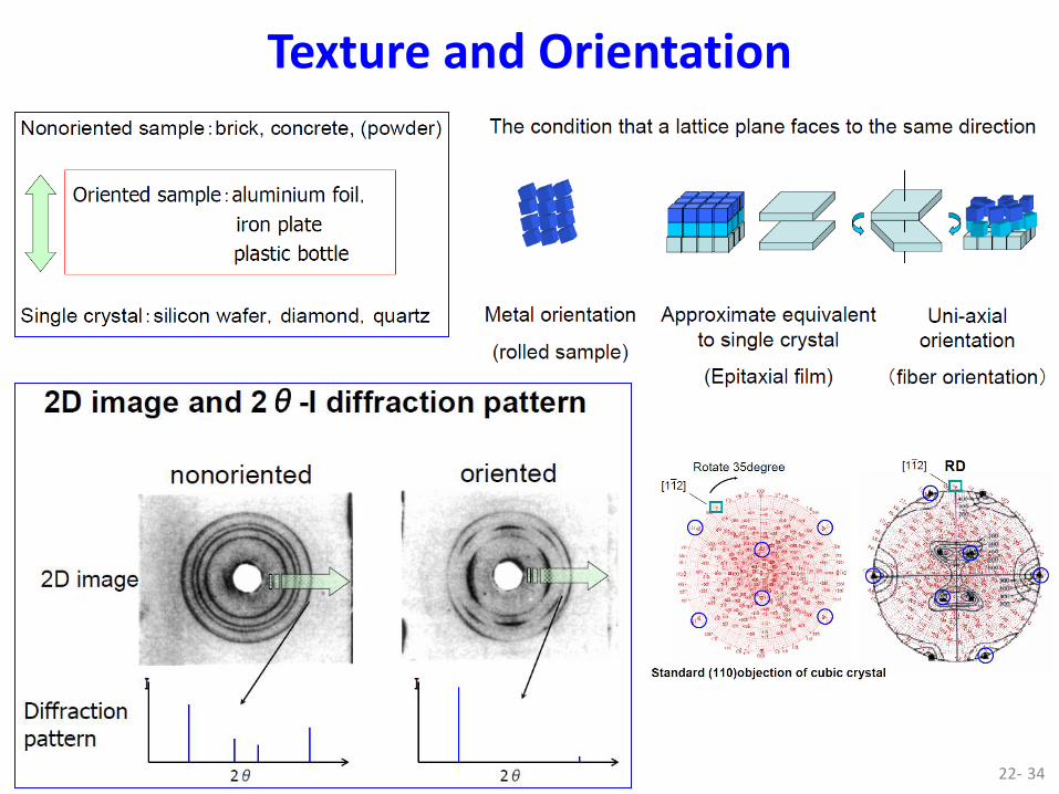
Texture and Orientation

22- 34

Crystallite Size

22- 35

Limitations of XRD

• Overlapping peaks – Due to the presence of other phases.

• Uncertainty in determining the peak positions – Associated with an unknown phase.

• Locating hydrogen atoms - Hydrogen atoms make extremely small contributions to the overall electron density > XRD is not a good technique for accurately locating H atom positions. Neutron diffraction is required b/c H atoms scatter neutrons as effectively as many other atoms.

• The need for single crystals – Materials that cannot be crystallised (e.g., glasses) or amorphous materials (e.g. some ceramics and polymers) cannot be investigated in detail by diffraction techniques.

22- 36

History (Triumph) of XRD - 4

• 1953: James Watson (1928- ) and Francis Crick (1916-2004) both at Cambridge U solved the DNA structure with the double helix – Nobel Prize in Physiology/Medicine 1962 shared with Maurice Wilkins (1916-2004, King’s College). It was the XRD work of Wilkins’ colleague at King’s College, Rosalind Franklin (1920-1958) who died of cancer at the age of 37 and before the Nobel Prize was awarded, that was often credited to this discovery.

• Franklin discovered that DNA could crystalize into two forms. Her boss John Randall gave form A to Franklin and form B to Wilkins and got them to solve their molecular structures.

• Franklin got photo 51. Wilkins showed Franklin’s data to Watson and Crick without her knowledge or consent.

22- 37

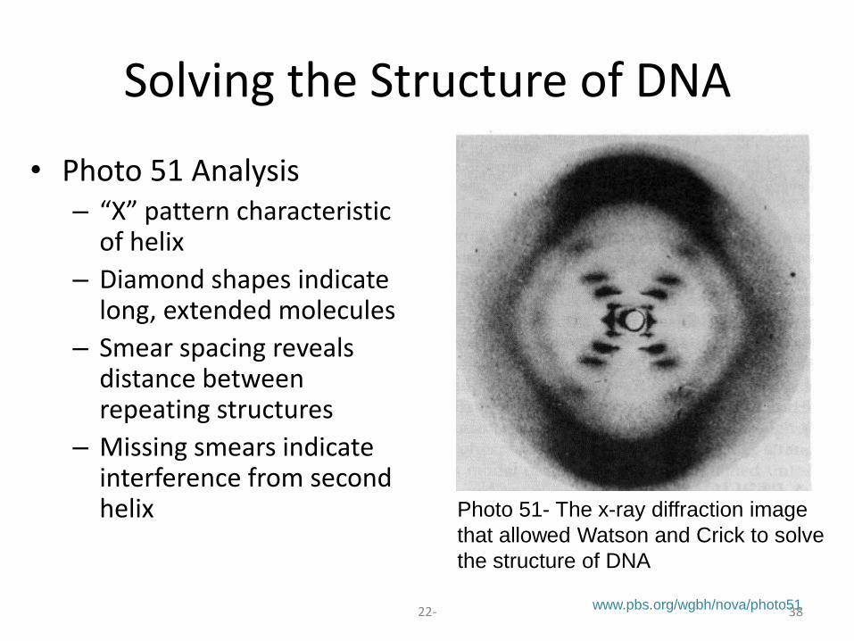
Solving the Structure of DNA

• Photo 51 Analysis – “X” pattern characteristic

of helix

– Diamond shapes indicate long, extended molecules

– Smear spacing reveals distance between repeating structures

– Missing smears indicate interference from second helix Photo 51- The x-ray diffraction image

that allowed Watson and Crick to solve

the structure of DNA

www.pbs.org/wgbh/nova/photo51 22- 38


Photo 51- The x-ray diffraction image




of helix



– Missing smears indicate interference from second helix







of helix






• Information Gained from Photo 51

– Double Helix

– Radius: 10 angstroms

– Distance between bases: 3.4 angstroms

– Distance per turn: 34 angstroms

• Combining Data with Other Information – DNA made from:

sugar

phosphates

4 nucleotides (A,C,G,T)

– Chargaff’s Rules %A=%T %G=%C

– Molecular Modeling

Watson & Crick’s model

22- 43

Homework 4A: Work through the following site: http://www.matter.org.uk/diffraction/x-ray/

i.e. answer the questions at the site.

For a Cu X-ray, what is the thickness for a Co specimen to totally block the X-ray?

Homework 4B: Work through the following site:

http://www.eserc.stonybrook.edu/ProjectJava/Bragg/

and use their Java app to determine at what theta when the intensity reaches maximum for (a) Lambda = 2 and Distance = 1.5, and (b) Lambda = 1.5 and Distance = 1.5.

22- 44

http://www.matter.org.uk/diffraction/x-ray/







lecture 22 - university of waterlooleung.uwaterloo.ca/mns/102/lect_2013/lect_22b.pdf · lecture 22...

Documents