High Risk Episodes and the Equity Size Premium∗

Naresh Bansal,a Robert A. Connolly,b and Chris Stiversc

a John Cook School of Business

Saint Louis University

b Kenan-Flagler Business School

University of North Carolina at Chapel Hill

c College of Business

University of Louisville

December 16, 2016

∗We thank Ric Colacito, Jennifer Conrad, Loan Dang, David Dubofsky, Christian Lundblad, Nick Gantchev,Topaz Prawito, Adam Reed, Jacob Sagi, Gill Segal, Guofu Zhou, and seminar participants at UNC-Chapel Hill,Saint Louis University, the University of Louisville, and the 2015 Financial Management Association meetingsfor helpful comments. Please address comments to Naresh Bansal (e-mail: nbansal@slu.edu; phone: (314) 977-7204; Robert Connolly (email: Robert Connolly@unc.edu; phone: (919) 962-0053); or to Chris Stivers (e-mail:chris.stivers@louisville.edu; phone: (502) 852-4829).

1

High Risk Episodes and the Equity Size Premium

Abstract

We find that the equity size premium is pervasively positive, sizable, and statistically significant

solely over periods that follow a high-risk month; defined as a month that ends with the expected

market volatility being in its top quintile. Following the other lower-risk months, the size premium

is essentially zero and statistically insignificant. Conditional CAPM alphas for Small-minus-Big

(SMB) long/short portfolio returns also exhibit a very similar risk-based contingent variation.

Concurrently, SMB returns are negative and reliably lower in the months leading up to our top-

quintile-volatility condition. Our results indicate a nonlinear positive intertemporal risk-return

relation for the equity size premium, seemingly attributed to high-risk episodes where small-cap

stocks face relatively higher market volatility-, illiquidity-, and default-risk. Our findings suggest

support for: (1) Acharya-Pedersen’s (2005) implication that persistent illiquidity shocks can

generate low concurrent returns and higher future returns, (2) Hahn-Lee’s (2006) and Kapadia’s

(2011) view that default risk has a role for understanding the size premium, and (3) Ang et al ’s

(2006) view that stocks with a more negative sensitivity to market volatility innovations should

have a higher risk premium.

JEL Classification: G11

Keywords: SMB premium, Volatility Risk, Illiquidity Risk, Default Risk, Intertemporal Risk-

Return Tradeoff.

1. Introduction

In this paper, we establish a striking new risk-based time-series regularity in the equity size

premium that bears on understanding the economic foundations of the size premium and its

time variation, as well as the intertemporal risk-return tradeoff in equity markets.1 Specifically,

over 1926 to 2014, we find that the equity size premium is pervasively positive, sizable, and

statistically significant solely over periods that follow a high-risk month; which we define as

a month that ends with the expected market volatility in its top quintile (or, a ‘top-quintile

volatility condition’). Following the other lower-risk months, the subsequent size premium is

essentially zero and statistically insignificant.2 To indicate the ‘expected market volatility’ in

our analysis, we rely on the CBOE’s option-derived S&P 500 implied volatility (VIX) for the

1990-2014 segment of our sample and a measure of recent realized volatility (RV) for our pre-1990

investigation. Our findings are robust to other measures.

This nonlinear intertemporal risk-to-return relation in the size premium is evident in the

subsequent 12-, 6-, 3-, and 1-month cumulative returns following the high-risk state. The

magnitude of this intertemporal variation seems striking. For example, over 1990-2014(1960-

1989)[1926-1959], the average 6-month Fama-French SMB cumulative return over months t + 1

to t+ 6 is +5.90%(+5.37%)[+7.59%] when the closing VIX(RV)[RV] for month t− 1 is above its

80th percentile; as compared to -0.16% (+0.81%)[+0.52%] following other times.

A similar contingent variation in SMB-type average returns is evident when the long small-

1The equity size premium refers to the tendency of small-cap stocks to earn higher average returns than large-cap stocks. A size premium has important implications for both investments and corporate finance, so it has beenstudied extensively; the literature on size in asset pricing dates back to least Banz (1981). Incorporation of the sizepremium into asset pricing models gained prominence after Fama and French (1992, 1993). Following Fama-Frenchand for brevity, we will commonly refer to the equity size premium also as the SMB (Small-minus-Big) premium.

2Time-variation in average SMB returns is well established in the literature; see, e.g., Van Dijk (2011) andAsness et al (2015). For example, while the average SMB premium is appreciable at +3.3% per annum over1927-2014, it was -1.6% over 1990-1999 versus +4.6% over 2009-2013. The striking time-variation, and especiallythe negative SMB returns in the 1990’s, have led some researchers to question a SMB premium. However, VanDijk argues that it is premature to claim the demise of the SMB premium, since “Stock returns are very noisy andstandard errors around estimates of the size premium are large, so it is not easy to tell whether the size effect islarger or smaller than it used to be.” (pg. 3263) The SMB factor-mimicking portfolio remains in Fama-French’srecent extension to a five-factor model; see Fama and French (2015, 2016).

1

cap side is defined as the third or fourth smallest value-weighted decile portfolio (with NYSE size

breakpoints); thus, our findings are not unique to microcap stocks. Further, we find a similar

SMB regularity for comparable European SMB-type stock returns, contingent on the German

VDAX equity-index implied volatility; thus, our findings are not unique to U.S. equity returns.

From a risk-adjusted-performance perspective, we also find that a top-quintile VIX/RV

predicts a conditional CAPM alpha that is: (1) sizably positive and statistically significant for

both SMB positions and small-cap portfolios, and (2) negative and statistically significant for the

largest size-decile portfolio. Following the other lower-risk periods, the comparable conditional

CAPM alphas are near zero and never statistically significant. These alpha findings not only fit

with the notion of the SMB premium being a CAPM anomaly; but also suggest that other risks,

beyond market-beta risk, are important for understanding our intertemporal SMB findings.

To further probe the underlying risks behind these time-series SMB regularities, we explore

dimensions of risk where appreciable size-based risk differentials are expected. Recent literature

is instructive with studies indicating that small-cap stocks face relatively higher illiquidity risk,

default risk, and stochastic-volatility risk; see Acharya and Pedersen (AP, 2005), Hahn and Lee

(HL, 2006), and Ang et al (2006). Such risks are generally thought of as having an episodic

nature, with risk spikes likely during significant economic crises. Consistent with this premise,

we find that our high-risk episodes have appreciably elevated illiquidity risk, default risk, and

stochastic-volatility risk. Thus, the episodic nature of the SMB premium, as suggested by our

findings, seems to intuitively fit the episodic nature of high-risk episodes for these type of risks.

Recent theory and evidence indicates that illiquidity risk can affect risk premia. AP’s (2005)

model predicts that a persistent negative shock to a security’s liquidity should be associated with

lower contemporaneous returns (as liquidity deteriorates over the risk buildup period) and higher

future returns (due to the elevated risk premium, attributed to the heightened risk/illiquidity

attained over the preceding risk buildup period). Since small-cap stocks have higher illiquidity

risk, AP’s theoretical predictions might bear on understanding our SMB return findings if the

2

illiquidity pricing influences are relatively more influential on small-cap stocks.

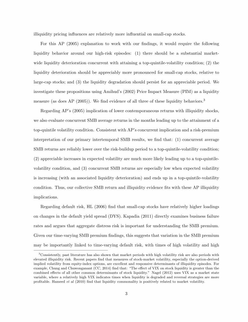
For this AP (2005) explanation to work with our findings, it would require the following

liquidity behavior around our high-risk episodes: (1) there should be a substantial market-

wide liquidity deterioration concurrent with attaining a top-quintile-volatility condition; (2) the

liquidity deterioration should be appreciably more pronounced for small-cap stocks, relative to

large-cap stocks; and (3) the liquidity degradation should persist for an appreciable period. We

investigate these propositions using Amihud’s (2002) Price Impact Measure (PIM) as a liquidity

measure (as does AP (2005)). We find evidence of all three of these liquidity behaviors.3

Regarding AP’s (2005) implication of lower contemporaneous returns with illiquidity shocks,

we also evaluate concurrent SMB average returns in the months leading up to the attainment of a

top-quintile volatility condition. Consistent with AP’s concurrent implication and a risk-premium

interpretation of our primary intertemporal SMB results, we find that: (1) concurrent average

SMB returns are reliably lower over the risk-buildup period to a top-quintile-volatility condition;

(2) appreciable increases in expected volatility are much more likely leading up to a top-quintile-

volatility condition, and (3) concurrent SMB returns are especially low when expected volatility

is increasing (with an associated liquidity deterioration) and ends up in a top-quintile-volatility

condition. Thus, our collective SMB return and illiquidity evidence fits with these AP illiquidity

implications.

Regarding default risk, HL (2006) find that small-cap stocks have relatively higher loadings

on changes in the default yield spread (DYS). Kapadia (2011) directly examines business failure

rates and argues that aggregate distress risk is important for understanding the SMB premium.

Given our time-varying SMB premium findings, this suggests that variation in the SMB premium

may be importantly linked to time-varying default risk, with times of high volatility and high

3Consistently, past literature has also shown that market periods with high volatility risk are also periods withelevated illiquidity risk. Recent papers find that measures of stock-market volatility, especially the option-derivedimplied volatility from equity-index options, are excellent and responsive determinants of illiquidity episodes. Forexample, Chung and Chuwonganant (CC, 2014) find that: “The effect of VIX on stock liquidity is greater than thecombined effects of all other common determinants of stock liquidity.” Nagel (2012) uses VIX as a market statevariable, where a relatively high VIX indicates times when liquidity is degraded and reversal strategies are moreprofitable. Hameed et al (2010) find that liquidity commonality is positively related to market volatility.

3

default risk generally coinciding.4 In our setting, we find that a high DYS also indicates a higher

subsequent SMB premium, but the DYS conditioning appreciably underperforms our volatility

conditioning. This finding suggests that size-based differences in time-varying default risk is a

likely contributor to our volatility-SMB findings, but is likely only part of the explanation.

Regarding stochastic-volatility risk, Ang et al (2006) find that stocks with a more negative

relation to market-volatility innovations have a higher risk premium. Over our sample, we confirm

that small-cap portfolio returns have an appreciably more negative sensitivity to market-volatility

innovations. Since expected volatility is also more variable around our high-risk episodes, this

also suggests a relatively higher small-cap risk premium with our high-risk episodes.

Our study also bears on the questions of the intertemporal risk-return relation in equity

markets. Campbell (1987) and Scruggs (1998) point out that the evaluation of a simple risk-

return relation in the equity market may be obscured by omitted state variables; variables that

are external to the stock market but influence the equity risk premium (e.g., Treasury yields).

Long-short equity positions, constructed from broad diversified portfolios that emphasize a sizable

systematic equity-risk differential, could mitigate the influence of omitted state variables (since

both sides of the long-short equity position should presumably be affected similarly). SMB

portfolios are long-short positions that have compelling size-based risk differentials that are

appreciably elevated during high-risk market episodes. Thus, a time-varying SMB premium

seems likely to provide a useful evaluation of the intertemporal equity risk-return tradeoff.

Our SMB findings indicate a positive nonlinear risk-return tradeoff in equity markets, as

linked to time-varying volatility, default, and illiquidity risk. This nonlinearity echoes elements of

recent studies that evaluate the intertemporal risk-return relation between market-level expected

volatility and the market risk premium; a positive risk-return tradeoff is indicated under some

4Relatedly, Jagannathan and Wang (1996) use a default yield spread as a proxy for time-variation in the marketrisk premium.

4

market conditions even if a simple linear relation is not reliably evident.5

In sum, our evidence and arguments suggest that a time-varying SMB premium is logical and

expected, with high-risk episodes (with appreciably elevated market-level volatility, illiquidity,

and default risk) predicting a relatively high subsequent SMB premium in a nonlinear manner.

Our findings fit with the appreciable time-variation in the SMB premium documented in the

literature, including the weak SMB performance over the mid-1990’s.6

This paper is organized as follows. Section 2 describes our data. Section 3 presents our main

intertemporal findings on the ‘expected volatility’-to-SMB linkage. Sections 4 and 5 provides

concurrent and intertemporal risk-based evidence to assist with interpretation of our primary

intertemporal SMB findings. Section 6 presents additional related evidence. Section 7 concludes.

2. Data

2.1. Sample Period Selection

We investigate two different sample periods primarily, which collectively span the recent 55 year

period: the 25-year period from 1990 to 2014, and the earlier 30-year period from 1960 to 1989.

Two considerations affect our choice of the sample period. First, the availability of the CBOE’s

implied Volatility Index (VIX), which is an important measure for our study (see Section 2.3),

drives our choice of the recent 1990-2014 sample period. Second, our earlier 1960-1989 sample

5See Section 2 in Adrian, et al. (2016) for an excellent discussion of theoretical models that generate nonlinearrisk-return tradeoffs. Scruggs (1998) and Ghysels, et al. (2005) provide excellent reviews of the empirical literaturethat studies the Merton market-level risk-return tradeoff prediction. Other related literature includes Rossi andTimmermann (2010), Brunnermeier and Pedersen (2009), Caballero and Krishnamurthy (2008), Weill (2007),Vayanos (2004), and Whitelaw (2000). None of these papers looks at the risk-return tradeoff for size-sortedlong/short portfolios, and we are unaware of any exploration of nonlinear risk-return tradeoffs involving other risksources besides the market factor.

6Our findings suggest that it is not surprising that SMB returns were poor over 1994 to 1998. By 1994, theVIX had been modest for some time (with an average end-of-month VIX of 13.5% over 1992-93) and the VIXremained modest through late 1997. In the context of our findings, this suggests a low SMB risk premium over1994-97. Then, in the fall of 1998 with the onset of the financial crisis associated with the Russian foreign-debtdefault, the VIX spiked from 24.8% to 44.3% over August 1998 and an SMB position lost over 15% that month.Subsequently, over 1999, an SMB position earned over +15% (following the late 1998 high-risk episode), consistentwith the pattern suggested by our findings.

5

is the subject period for important early SMB research. For example, Fama and French (1992)

studied the 1962-1989 period; and Fama and French (1993) studied the 1963-1991 period. Our

1990-2014 sample roughly acts as a post-discovery period in relation to these studies. Accordingly,

we report our results separately for the two sample periods (as opposed to reporting results for

collective 55-year period). For some analysis, we evaluate the 50-year period over 1965-2014 as

a single longer duration sample, using RV and other conditioning variables.

We also briefly investigate SMB returns over July 1926 to December 1959 to evaluate whether

our primary findings are also evident in this earlier historical segment. We only briefly evaluate

the 1926-1959 period in a minor complementary role because: (1) the extreme volatility around

the 1930’s Great Depression could result in this very distant and extreme period having an

undesirably large influence on our primary results; (2) possible market distortions associated

with the World War II period, and (3) the above-mentioned historical role of the 1960-1990

period in early SMB research.

2.2. SMB-type Portfolios

To contrast small caps vs. large caps, we study nine different small-minus-big portfolio positions.

First, and most importantly, we study the Fama-French SMB factor-mimicking portfolio. Addi-

tionally, we study the return difference between each of the four smallest market-cap-based decile

portfolios (both value-weighted and equal-weighted) and the largest size-based decile portfolio

(value-weighted). The data for the Fama-French SMB and the various market-cap-based decile

portfolios are taken from the French data library.

Examining the four smallest size-based deciles ensures that our results are not solely driven

by thinly traded micro-cap stocks. It is important to note that these decile portfolios use the

NYSE-based market capitalization breakpoints, as explained in the French data library. Thus,

the smallest decile contains far more stocks than any of the remaining deciles since July 1963.7 For

7Prior to July 1963, each of the French size-based decile portfolios contains roughly an equal number of stocks.

6

instance, from July 1963 to our sample end date of December 2014, the smallest size-based decile

contains 47.1% of the total number of firms, and the smallest two size-based deciles contains 59.1%

of the total firms, on average. Accordingly, the decile-three and decile-four size portfolios contain

sizable small-cap stocks (rather than micro-cap stocks) with an average market capitalization

per stock of $941 million and $1.63 billion, respectively, in December 2014. For brevity, our

main text reports results primarily for the value-weighted portfolios; results for equal-weighted

portfolios are presented in our appendix.

2.3. Expected Market-Level Equity Volatility

Our primary measures of expected ‘equity market volatility’ differs across our two sample periods.

For the 1990-2014 sample period, our primary measure is the VIX since it has been shown that

VIX not only contains highly reliable information about the subsequent market volatility, but it

is also a very useful determinant for market liquidity.8 For the earlier 1960-1989 sample, since

neither VIX nor any other comparable implied-volatility index is available, our measure is the

lagged ‘realized volatility’ (RV) that is estimated from daily stock market returns over the prior

66-trading days.9 We choose RV since, given the time-series volatility clustering in stock-market

returns, the time-series models of expected volatility routinely rely on recent lagged return shocks.

Figure 1 displays the time series of VIX over 1990-2014 (Panel A) and our RV over 1960-1989

(Panel B).

Our empirical work relies on the notion that our primary equity-volatility variables contain

substantial and reliable information about the subsequent stock market volatility. We investigate

8Beyond the previously-discussed CC (2014) and Nagel (2012), other papers suggest a liquidity impairmentwith high VIX. Gromb and Vayanos (2002) and Brunnermeier and Pedersen (2009) predict that higher equityreturn volatility will cause funding constraints to bind for market makers which impairs their ability to provideliquidity. In Garleanu and Pedersen (2007) and Adrian and Shin (2010), higher VIX leads financial institutionswith risk management programs to reduce their market making activities as part of a broader effort to reduce riskexposure.

9For computing RV, we sum the squared daily aggregate stock market returns (proxied by returns on theCRSP value-weighted stock index). In computing volatility, we do not demean the returns before squaring, whichrecognizes that a daily expected return should be essentially zero. We also evaluate 22-trading-day and 44-trading-day RV measures and find they perform similarly but modestly weaker in our setting than our featured66-trading-day RV.

7

this premise by using the lagged VIX and RV as explanatory variables for the subsequent realized

stock-market volatility. We confirm the forward-looking volatility information in these variables;

both for VIX over 1990-2014 and our RV for 1960-1989. For brevity, details are relegated to

Appendix A1.10

Finally, we also construct a high-frequency Realized Volatility (RV), calculated from 5-minute

S&P 500 ETF returns, for secondary aspects of our analysis. See Appendix A3 for details on our

high-frequency RV construction.

2.4. Price Impact Measure (PIM)

For each of the size-based decile stock portfolios, we calculate portfolio-level measures of Amihud’s

(2002) Price Impact Measure (PIM). We use the PIM measure as it is widely used in the

literature as a quality liquidity measure that can be estimated over long samples (see AP (2005),

for example). Goyenko, Holden, and Trzcinka (2009) compare performance of several different

liquidity measures and find that the Amihud PIM measure does well in measuring price impact.

For the portfolio-level PIM, we aggregate the PIM values for each individual stock in the

portfolio, as detailed in Appendix A2. We aggregate the individual stock PIM’s using both a

value-weighting and equal-weighting method. As for our portfolio returns results, we primarily

report on the value-weighted portfolio PIM’s, but also present equal-weighted results in our

appendix. The size breakpoints are based on the NYSE breakpoints, consistent with the portfolio

returns per Section 2.2.

3. The Intertemporal Volatility-to-SMB Empirical Relation

We now turn to our main empirical analysis. Our focus here is on the intertemporal relation

between the stock market’s expected return volatility and the subsequent SMB premium. In

10Also, see Christensen and Prabhala (1998) and Blair, Poon, and Taylor (2001) for supportive evidence on theinformational content of equity-index implied volatility.

8

later sections, we recognize and investigate other dimensions of risk that are also likely to be

elevated during periods of high expected volatility.

In our intertemporal investigation, the featured dependent variable is a cumulative return of

an SMB-type portfolio over months t+ 1 to t+ j, computed as the difference in the cumulative

returns of a small-cap and large-cap portfolio over this period. The time indicator variable j

is either 3, 6, or 12; representing the 3-, 6-, and 12-month return horizons, respectively. The

explanatory variable is based on the ‘expected stock-market volatility’ at the close of month t−1.

Our method skips the month t between the explanatory variable and the subsequent dependent

variable for several reasons. First, the skip-a-month method has largely become standard in the

momentum literature to avoid microstructure concerns between the ranking and holding period.

Second, Bali et. al. (2014) argue that the price response to liquidity shocks may be delayed

over several months, perhaps due to investor inattention in small caps. Consistent with this

premise, we show later that the small-cap portfolios are related to both the concurrent and first

lag VIX-shock, which supports the need to skip a month (see Section 4.2).

We perform separate estimations for 3-month, 6-month, and 12-month cumulative returns for

two primary reasons. First, these horizons are prevalent in the finance literature that investigates

time-varying risk premia linked to a lagged state variable. Second, our Section 5 provides evidence

of elevated risk persistence several months following the attainment of a high volatility condition.

Consider that the autocorrelation behavior of monthly VIX values indicates a half-life for VIX

shocks of about 4.3 months, with a first-order autocorrelation of 0.85.

This section is organized as follows. We first evaluate both a traditional linear risk-return re-

lation (Section 3.1) and a nonlinear risk-return relation (Sections 3.2, 3.3, and 3.4). The nonlinear

specifications are motivated by the notion of high-risk volatility episodes, where small-cap stocks

especially are likely to face appreciably elevated illiquidity-, default, and/or stochastic-volatility

risk. Next, Section 3.5 shows that our volatility-to-SMB findings survive risk-adjustment using a

conditional CAPM alpha approach. Section 3.6 documents the same SMB regularity in U.S.

9

equity returns over 1926-1959. Section 3.7 documents similar volatility-to-SMB findings in

European stock returns. Finally, Section 3.8 provide a series of additional robustness evidence.

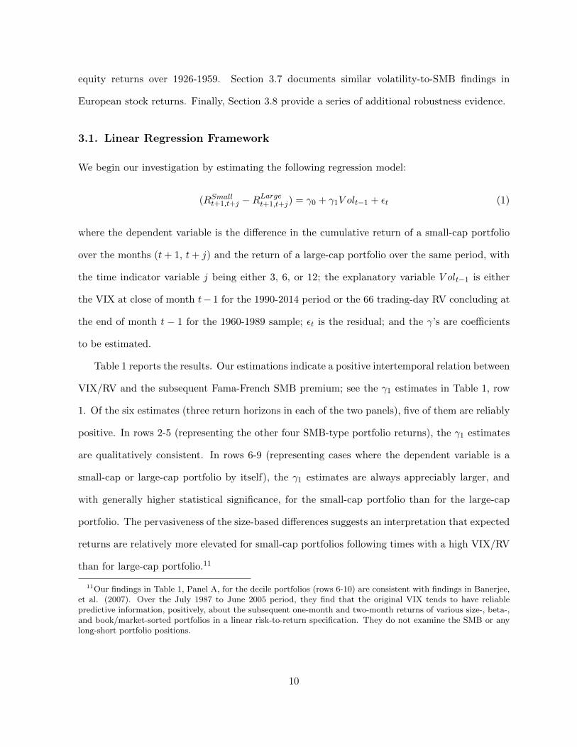
3.1. Linear Regression Framework

We begin our investigation by estimating the following regression model:

(RSmallt+1,t+j −R

Larget+1,t+j) = γ0 + γ1V olt−1 + εt (1)

where the dependent variable is the difference in the cumulative return of a small-cap portfolio

over the months (t+ 1, t+ j) and the return of a large-cap portfolio over the same period, with

the time indicator variable j being either 3, 6, or 12; the explanatory variable V olt−1 is either

the VIX at close of month t− 1 for the 1990-2014 period or the 66 trading-day RV concluding at

the end of month t − 1 for the 1960-1989 sample; εt is the residual; and the γ’s are coefficients

to be estimated.

Table 1 reports the results. Our estimations indicate a positive intertemporal relation between

VIX/RV and the subsequent Fama-French SMB premium; see the γ1 estimates in Table 1, row

1. Of the six estimates (three return horizons in each of the two panels), five of them are reliably

positive. In rows 2-5 (representing the other four SMB-type portfolio returns), the γ1 estimates

are qualitatively consistent. In rows 6-9 (representing cases where the dependent variable is a

small-cap or large-cap portfolio by itself), the γ1 estimates are always appreciably larger, and

with generally higher statistical significance, for the small-cap portfolio than for the large-cap

portfolio. The pervasiveness of the size-based differences suggests an interpretation that expected

returns are relatively more elevated for small-cap portfolios following times with a high VIX/RV

than for large-cap portfolio.11

11Our findings in Table 1, Panel A, for the decile portfolios (rows 6-10) are consistent with findings in Banerjee,et al. (2007). Over the July 1987 to June 2005 period, they find that the original VIX tends to have reliablepredictive information, positively, about the subsequent one-month and two-month returns of various size-, beta-,and book/market-sorted portfolios in a linear risk-to-return specification. They do not examine the SMB or anylong-short portfolio positions.

10

3.2. Average SMB Returns for Decile Subsets, Based on the Lagged VIX/RV

While the Table 1 results are interesting, the specification implies a continuous linear relation

between VIX/RV and the subsequent SMB premia. However, as we document in Sections 4 and

5, episodes with especially high expected market volatility also tend to have higher illiquidity-,

default-, and stochastic-volatility risk; with small-cap stocks being especially sensitive to such

elevated risks. Such episodes are generally associated with some significant underlying economic

or political crisis; see our Figure 1. Thus, the volatility-to-SMB relation might instead be better

represented by a nonlinear relation especially linked to a particularly high VIX/RV.

Accordingly, we evaluate the monotonicity of the intertemporal volatilityto-SMB relation by

stratifying the sample into ten deciles, based on the lagged VIX/RV. The decile approach should

clearly evaluate whether the volatility-to-SMB relation can be described as more monotonic

(consistent with the linear specification in Table 1), or more concentrated in one area of the

VIX/RV distribution (implying a nonlinear relation). A decile approach provides a nice level of

stratification, while still ensuring a reasonable number of observations for each subset grouping.

We estimate the following regression model:

(RSmallt+1,t+j −R

Larget+1,t+j) = γ1Dum

V olDec1t−1 + γ2Dum

V olDec2t−1 + ....+ γ10Dum

V olDec10t−1 + εt (2)

where the explanatory variables are 10 different dummy variables depending upon which decile

the VIX/RV value from month t− 1 fell in, and the other terms are as defined for equation (1).

Thus, the estimated coefficient on each dummy variables provides the conditional average return

for the SMB portfolio, dependent upon the VIX/RV decile.

Table 2 reports the results. We report both the unconditional mean return (column labeled

‘All’) and the conditional average returns (columns labeled ‘Dc 1’ to ‘Dc 10’). We report separate

results for 1990-2014 (contingent on the lagged VIX decile) and for 1960-1989 (contingent on the

lagged RV decile). Estimates are reported for the five SMB-type portfolios (rows 1 to 5) and on

different size-based portfolios themselves (rows 6 to 9).

11

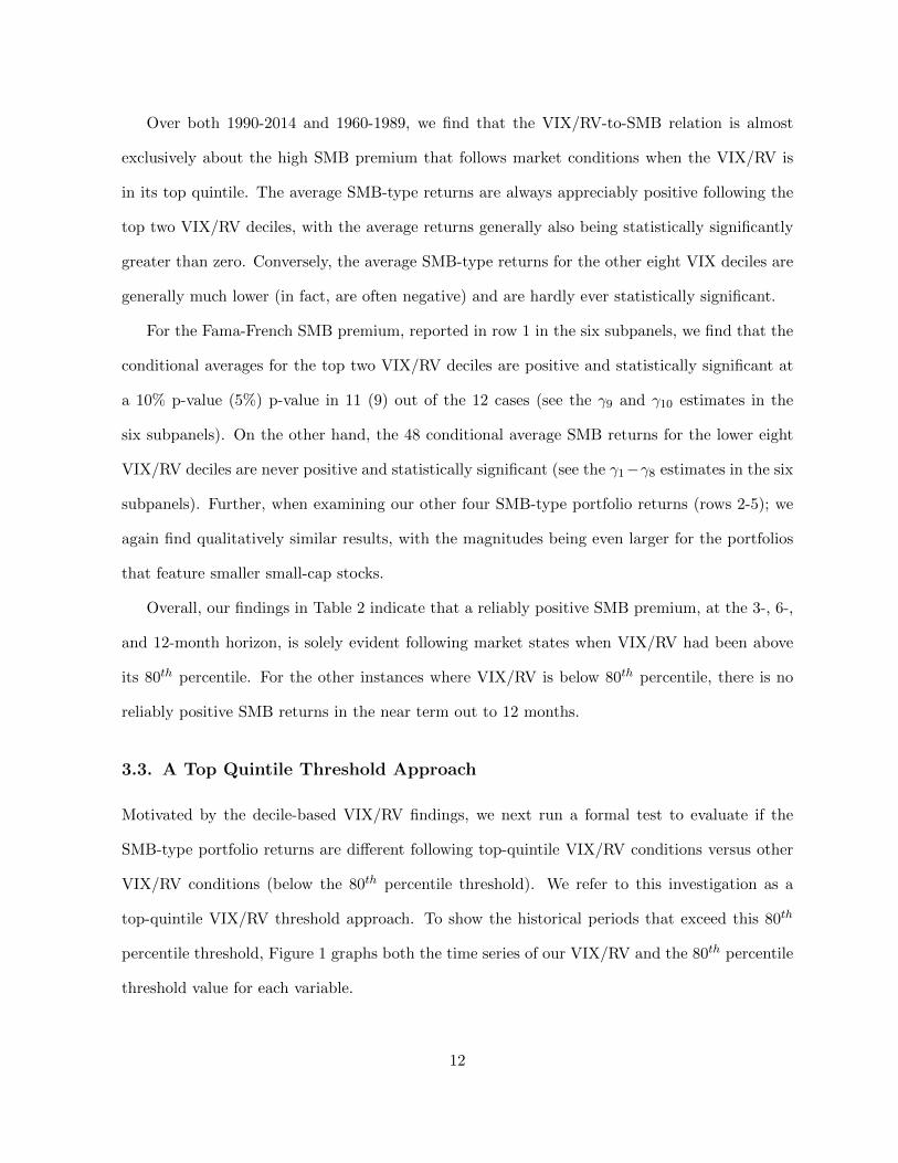
Over both 1990-2014 and 1960-1989, we find that the VIX/RV-to-SMB relation is almost

exclusively about the high SMB premium that follows market conditions when the VIX/RV is

in its top quintile. The average SMB-type returns are always appreciably positive following the

top two VIX/RV deciles, with the average returns generally also being statistically significantly

greater than zero. Conversely, the average SMB-type returns for the other eight VIX deciles are

generally much lower (in fact, are often negative) and are hardly ever statistically significant.

For the Fama-French SMB premium, reported in row 1 in the six subpanels, we find that the

conditional averages for the top two VIX/RV deciles are positive and statistically significant at

a 10% p-value (5%) p-value in 11 (9) out of the 12 cases (see the γ9 and γ10 estimates in the

six subpanels). On the other hand, the 48 conditional average SMB returns for the lower eight

VIX/RV deciles are never positive and statistically significant (see the γ1−γ8 estimates in the six

subpanels). Further, when examining our other four SMB-type portfolio returns (rows 2-5); we

again find qualitatively similar results, with the magnitudes being even larger for the portfolios

that feature smaller small-cap stocks.

Overall, our findings in Table 2 indicate that a reliably positive SMB premium, at the 3-, 6-,

and 12-month horizon, is solely evident following market states when VIX/RV had been above

its 80th percentile. For the other instances where VIX/RV is below 80th percentile, there is no

reliably positive SMB returns in the near term out to 12 months.

3.3. A Top Quintile Threshold Approach

Motivated by the decile-based VIX/RV findings, we next run a formal test to evaluate if the

SMB-type portfolio returns are different following top-quintile VIX/RV conditions versus other

VIX/RV conditions (below the 80th percentile threshold). We refer to this investigation as a

top-quintile VIX/RV threshold approach. To show the historical periods that exceed this 80th

percentile threshold, Figure 1 graphs both the time series of our VIX/RV and the 80th percentile

threshold value for each variable.

12

We estimate the following regression model:

(RSmallt+1,t+j −R

Larget+1,t+j) = ψ0 + ψ1Dummy

V ol<80thPctlt−1 + εt (3)

where the explanatory variable is a dummy variable that equals one if the V olt−1 level is less than

its 80th percentile; the ψ’s are coefficients to be estimated; and the other terms are as defined

for equation (1).

Table 3 reports the estimation results, with Panels A to C reporting on the 3-month, 6-month

and 12-month returns, respectively. For both our 1990-2014 and 1960-1989 sample, the results

are striking. For the Fama-French SMB portfolio and the other four value-weighted SMB-type

positions in the six subpanels, the SMB premium is sizably positive and statistically significant

following times when VIX/RV is in its top quintile for all 30 cases (see column 2 in the table,

with the ψ0 coefficient). Next, the ψ1 coefficients are negative in all 30 cases and statistically

significant in 29 of the 30 cases, indicating that the size premium is reliably different between

the higher- and lower-risk periods. Finally, the SMB premium is not positive and statistically

significant for any of the 30 cases that follow a lower VIX/RV (< 80th percentile), even though

this condition makes up 80% of the observations (see column 4 in the table).

We also note the following. For all six cases for the Fama-French SMB portfolio in row-1

(three return horizons over our two primary sample periods), the R2 value for the regression

with the single dummy variable in Table 3 is greater than the comparable R2 value for the linear

continuous regression in Table 1. In our view, this seems striking and supports the efficacy of

such a nonlinear approach.

Overall, the results in Tables 2 and 3 indicate that a traditional linear regression approach in

measuring an intertemporal risk-to-SMB-premia approach is substantially misspecified. Instead,

there is a striking and reliable nonlinear intertemporal risk-to-return relation, characterized by

the very high small-cap returns that tend to follow a high VIX/RV value.

13

3.4. Comparable Real-Time Method

In Tables 2 and 3, the volatility value for each month is categorized into a ‘volatility decile’ based

on the entire volatility distribution over the respective sample period. This means, of course,

that the classification is not available in real time because the complete distribution must be

known. In this subsection, we report on a similar top-quintile-volatility exercise as in Section

3.3, but where the classification method could be implemented in real time.

We use the distribution of the prior 180 months of our RV measure over months t − 1 to

t − 180 to determine whether month t − 1 is in a top-quintile-volatility condition, in terms of

evaluating the future SMB returns over months t + 1 to t + j. We evaluate the 50-year period

over 1965-2014, so the first lagged reference distribution is over 1950-1964.12 We use the lagged,

rolling RV for classification over the entire period to provide continuity, rather than shifting to

VIX in 1990. Additionally, our investigation here serves to evaluate a long 50-year sample period

in a single analysis, rather than evaluating pre- and post-1990 separately.

We report our findings in Table 4. For the future 3- (6-) [12-] month SMB returns, the average

Fama-French SMB returns are +3.23% (+5.63%) [+8.97%] following a top-quintile-volatility

month versus -0.06% (+0.17%) [+1.24%] for the remainder of the months. The differences in

means are statistically significant at a 0.2% p-value, or better, for all three horizons. We conclude

our findings are robust when using a real-time implementable volatility classification method.

3.5. CAPM Alphas, Conditional on ‘Top-Quintile Volatility’ Market State

All our analysis so far has focused solely on conditional average returns for the various SMB

and size portfolios. In this subsection, we evaluate risk-adjusted performance by investigating

conditional CAPM alphas for SMB portfolios (and small-cap and large-cap portfolios), instead of

12We choose a long 15-year lagged reference distribution period to ensure a lengthy comparison period thatgenerally includes at least two recessions. Our evaluation period commences in 1965 here, rather than 1960,because we later perform a comparable analysis using a default yield spread that relies on the 10-year TreasuryConstant Maturity yield. This yield is first available in 1954, so a later 1965 start date provides a reasonably longlagged reference distribution period for the DYS. See Section 6.1.

14

conditional average returns. Our motivation here is that if CAPM alphas also exhibit a similar

intertemporal pattern (contingent upon a top-quintile VIX/RV), then that would be a strong

indicator of a role for other risks beyond the traditional market-beta CAPM risk.

We evaluate conditional CAPM alphas as follows. First, we regress the monthly SMB or size-

based portfolio’s excess returns against the concurrent monthly excess market return, and retain

the sum of the intercept and the residual.13 This sum represents the component of the portfolio

return that is not linked to movements in the market return. We then re-estimate a modified

version of equation (3) that use this non-market component of the portfolio’s return in place

of the total return as the dependent variable. The monthly non-market-return components are

cumulated to evaluate the 3-, 6-, and 12-month values. In our setting, the conditional averages

of the non-market component of the return are interpreted as conditional alphas.

Table 5 reports the results. Following our top-quintile-volatility condition, the state-contingent

alphas for the SMB and small-cap portfolios (column 2) are all positive and sizable, with statis-

tical significance for 23 of the 24 cases. Following the other lower-risk months, the conditional

alphas are small and never even close to statistically significant (column 4). Thus, our state-

contingent findings of abnormally high subsequent SMB returns (and small-cap returns) following

a top-quintile-volatility month are also reliably evident after controlling for the traditional CAPM

market-beta risk.

For the SMB and small-cap portfolios, we note that the estimated conditional alphas following

our high-risk months are smaller in magnitude than the comparable conditional average returns

in Table 3. For the SMB, the six ψ0’s in Table 5 are about 67% as large, on average, as the

comparable coefficients in Table 3. This comparison suggests that the traditional market-beta

risk is a partial contributor towards understanding the patterns in Table 3.14

13We use the risk-free return and ‘market-minus-risk-free’ return from the French data library. Our specificationdiscussed here estimates a single fixed beta over the sample. We also evaluated a market-model that allowed fora different state-contingent market-beta following our top-quintile-volatility state; but we found that the state-contingent difference in betas is small and never statistically significant.

14In Appendix A8, we directly report on the estimated market-betas for our various portfolios and show that anSMB position does face a sizable and statistically significant degree of traditional CAPM market-beta risk.

15

Finally, we highlight one other finding in Table 5. For the large-cap portfolio, we find that:

(i) the conditional alphas following a top-quintile-volatility month are always negative, with

statistical significance for five of the six cases (ψ0 in row 5, column 2); and (ii) the lower-volatility

alphas are greater than the top-quintile-volatility alphas, with statistically significant differences

in five of the six cases (ψ1 in row 5, column 3).

Thus, our findings indicate that the conditional alphas following a top-quintile-volatility

month are both reliably negative for the large-cap portfolio and reliably positive for the small-

cap portfolios. These combined results fit with the view that our high-risk episodes include

a substantial size-based differential in other risks beyond CAPM market-beta risk, which we

evaluate in later sections.

3.6. SMB Returns following High-Risk Periods over 1926 to 1959

We also repeat the volatility-to-SMB analysis, as in Table 3, for the Fama-French U.S. SMB

returns over July 1926 to December 1959. As we did for the 1960-1989 segment of our sample,

our volatility measure is a rolling 66-trading-day RV constructed from daily CRSP value-weighted

equity index returns. For this earlier period, we find qualitatively similar results to those in Table

3. Following a top-quintile-volatility month, we find that the subsequent 3-month (6-month) [12-

month] SMB average return is 4.59% (7.59%) [14.05%]. Conversely, following the other 80%

of the time for the lower-volatility market condition, we find that the subsequent 3-month (6-

month) [12-month] SMB average return is near zero at 0.08% (0.52%) [1.45%]. These differences

in means are statistically significant at better than a 10% p-value for all three horizons. This

evidence further supports the generality of our primary volatility-to-SMB findings.

3.7. International Evidence

We also use international data to probe the pervasiveness of our volatility-to-SMB findings. We

repeat our Table 3 analysis with a European SMB-type return replacing the U.S. SMB returns

16

and the implied volatility from the German DAX index (VDAX) replacing the U.S. VIX. For

the European SMB-type returns, we use: (i) the European SMB returns from the French data

library over January 1992 to December 2015, and (ii) SMB-type returns defined as the total

return difference between the European Small-Cap MSCI equity index and the European Large-

cap MSCI equity index over January 2001 to December 2015. Table 6 reports the results. Overall,

we find qualitatively consistent European results with statistical significance evident in all but

one case for the estimated ψ0 and ψ1 coefficients.

3.8. Additional Investigation and Robustness Checks

To further probe the generality and robustness of the intertemporal volatility-to-SMB regularity,

we repeat our Table 3 investigation in four different ways. For brevity, the detailed results are

reported in Appendices A3 to A7, respectively.

First, we repeat our Table 3 investigation over the following one-half subperiods for our two

primary samples: 1960:01-1974:12, 1975:01-1989:12, 1990:01-2002:06, and 2002:07-2014:12. We

find that the top-quintile VIX/RV-to-SMB patterns are qualitatively evident in each subperiod,

although the estimated ψ0’s and ψ1’s are not always statistically significant; see Appendix A3.

Second, so far, we have examined value-weighted portfolios. Under an illiquidity-based

explanation, our view is that the intertemporal VIX/RV-to-SMB relation should be of even

greater magnitude for the equal-weighted small-cap portfolios. Accordingly, we repeat the

empirical exercise in Table 3 with the top-quintile VIX/RV empirical approach, but with the

equal-weighted small-cap portfolios (R1e to R4e) replacing the value-weighted portfolios. Across

the board, we find similar qualitative VIX/RV-to-SMB patterns for the equal-weighted small-

cap portfolios. Further, the estimated ψ0 and ψ1 coefficients in equation (3) are even larger in

magnitude for the equal-weighted portfolios; see Appendix A4.

Third, we repeat the VIX/RV-to-SMB analysis, as in Table 3, but with one-month returns

as the dependent variable; see Appendix A5. We are interested in one-month returns because:

17

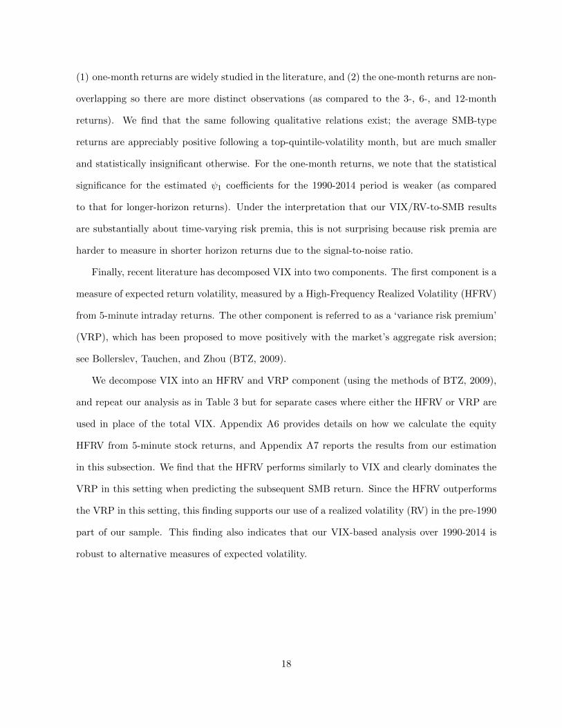
(1) one-month returns are widely studied in the literature, and (2) the one-month returns are non-

overlapping so there are more distinct observations (as compared to the 3-, 6-, and 12-month

returns). We find that the same following qualitative relations exist; the average SMB-type

returns are appreciably positive following a top-quintile-volatility month, but are much smaller

and statistically insignificant otherwise. For the one-month returns, we note that the statistical

significance for the estimated ψ1 coefficients for the 1990-2014 period is weaker (as compared

to that for longer-horizon returns). Under the interpretation that our VIX/RV-to-SMB results

are substantially about time-varying risk premia, this is not surprising because risk premia are

harder to measure in shorter horizon returns due to the signal-to-noise ratio.

Finally, recent literature has decomposed VIX into two components. The first component is a

measure of expected return volatility, measured by a High-Frequency Realized Volatility (HFRV)

from 5-minute intraday returns. The other component is referred to as a ‘variance risk premium’

(VRP), which has been proposed to move positively with the market’s aggregate risk aversion;

see Bollerslev, Tauchen, and Zhou (BTZ, 2009).

We decompose VIX into an HFRV and VRP component (using the methods of BTZ, 2009),

and repeat our analysis as in Table 3 but for separate cases where either the HFRV or VRP are

used in place of the total VIX. Appendix A6 provides details on how we calculate the equity

HFRV from 5-minute stock returns, and Appendix A7 reports the results from our estimation

in this subsection. We find that the HFRV performs similarly to VIX and clearly dominates the

VRP in this setting when predicting the subsequent SMB return. Since the HFRV outperforms

the VRP in this setting, this finding supports our use of a realized volatility (RV) in the pre-1990

part of our sample. This finding also indicates that our VIX-based analysis over 1990-2014 is

robust to alternative measures of expected volatility.

18

4. SMB Risk & Returns Coincident with the Buildup to a Top-

Quintile Volatility Condition

In this section, we investigate SMB risk and returns coincident with the buildup to a top-

quintile market volatility condition. Our concurrent investigation here supplements our primary

intertemporal investigation in Section 3, since the concurrent risk-return relation should assist

in interpretation. Our investigation includes volatility-, illiquidity-, and default risk.

To motivate further this section, consider arguments in French, Schwert, and Stambaugh

(FSS, 1987) and AP (2005). As part of their study of the intertemporal risk-return relation in

the equity market, FSS also investigate the concurrent risk-return relation. They find evidence

of a negative concurrent relation between stock market returns and innovations in expected

volatility, which is interpreted as indirect evidence of a positive intertemporal relation between

expected volatility and the subsequent risk premia. Next, AP’s asset-pricing model predicts that

a persistent negative shock to a security’s liquidity should result in low contemporaneous returns.

The general premise in such studies is that increased risk can induce a higher risk premium: prices

fall contemporaneously to reflect the higher forward-looking risk premium. Then, the negative

contemporaneous returns are followed by higher subsequent average returns as investors are paid

to bear the elevated risk.

It seems plausible that small-cap stocks would face relatively higher increases in risk (relative

to large caps) in the period leading up to the attainment of a top-quintile volatility condition.

Such increased risk could include volatility risk, illiquidity risk, and default risk. If so, under

an ‘interemporal risk-return tradeoff’ interpretation of our primary volatility-to-SMB findings in

Section 3, we would expect SMB returns coincident with the risk buildup to be relatively low.

In Section 4.1, we show exactly that.

This remainder of this section evaluates other dimensions of concurrent SMB risk. Section

4.2 shows that SMB returns load negatively on VIX innovations, indicating that small-cap stocks

have greater negative sensitivity to market-level volatility increases. Next, Section 4.3 shows

19

that liquidity degrades for both large-cap and small-cap stocks around the attainment of a top-

quintile volatility condition, but there is appreciably greater degradation for small-caps. Finally,

Section 4.4 documents that the default yield spread has both a markedly higher level and higher

variability leading up to a top-quintile volatility condition, indicative that default risk is also

higher for our high-risk episodes.

4.1. SMB Average Returns Preceding a Top-Quintile Volatility Condition

This subsection evaluates the behavior of SMB returns and expected-volatility innovations in the

period leading up to the attainment of a top-quintile-volatility condition at the end of month

t− 1. Following from Section 3, we focus on the top quintile of expected volatility.

We begin by estimating average SMB portfolio returns for the subset of observations that

precede a top-quintile-volatility condition. When month t − 1 ends in a top-quintile-volatility

condition, we calculate both the average one-month returns over month t − 1 and the average

cumulative two-month returns over months t−2 and t−1. We use a dummy variable in a regression

similar to equation (3) to calculate the average returns and the corresponding t-statistics, but

with the different timing described above.

Table 7, Panel A, reports the results. In all cases, we find that the average SMB returns are

negative in the months prior to attaining the top-quintile-volatility condition (column 2), and

that these negative average SMB returns are reliably lower than the average SMB returns in

other times (columns 3 and 4).

Next, an intertemporal risk-return tradeoff interpretation for our primary SMB findings in

Section 3 would also suggest that the prices of small-cap stocks would be especially adversely

impacted over months when both the expected-volatility increases appreciably and ends up in a

high risk environment (relative to large-cap stocks). To evaluate this proposition, Table 7, Panel

B, reports on the average returns for the following subsets of observations: (a) one-month returns

over month t− 1, when month t− 1 ends in a top-quintile-volatility condition and when month

20

t − 1 also has a top-quartile increase in the expected-volatility over the month (rows 1 to 4);

and (b) cumulative two-month returns over month t− 2 and t− 1, when month t− 1 ends in a

top-quintile-volatility conditions and when the two-month period over months t−2 to t−1 has a

top-quartile increase in the expected-volatility. Again, we use a dummy variable in a regression

similar to equation (3) to calculate the average returns and the corresponding t-statistics, but

with the conditional dummy variable chosen to meet the above two conditions.

The results in Panel B indicate that: (1) the average SMB returns for the observations that

meet the above two conditions (column two) are sizably and highly reliably negative; and (2)

average SMB returns for other periods are positive and reliably different (columns 3 and 4).

The negative average returns in Panel B, column-2, are about 3 times (2 times) the comparable

negative returns in Panel A, column-2, over 1990-2014 (1960-1989). We also note that about

41% to 62% of the months leading up to a top-quintile volatility condition are also times with a

top-quartile volatility increase.15

Finally, Table 7, Panel C, evaluates average SMB returns for the months that lead-up to a top-

quintile volatility condition but do not also have a corresponding top-quartile volatility increase.

In Panel C, we note that none of the estimated ψ0 or ψ1 coefficients for the SMB returns are

sizable or statistically significant for this variation. When combined with the Panel B results,

this indicates that there is no reliable difference in small-cap and large-cap returns when leading

up to the top-quintile-volatility condition unless there is also an appreciable expected-volatility

increase.

To sum up, when combined with our primary findings in Section 3, the evidence in Table

7 fits with the concept of: (1) a contemporaneous negative SMB pricing influence as the risk

builds up and the risk premium increases; and (2) followed by higher average SMB returns later,

15Each subpanel reports the percentage of times that meets the column-two condition, which ranges from 8.3%of the time for the 1990-2014 sample for the month t − 1 period (Panel B.1) to 12.5% of the time for 2-monthreturns for the 1960-1989 sample (Panel B.2). Since column two is capped at 20% of the observations with thecore top-quintile-volatility condition, these proportion translate to about 41% to 62% of the high-volatility-levelconditions being preceded by top-quartile volatility increases.

21

intertemporally, which reflects the elevated risk premium.

4.2. Stochastic Market Volatility Risk

In our prior subsection, we found that substantial increases in VIX/RV are much more likely in

the risk-buildup period that just precedes the attainment of a top-quintile volatility condition.

In this subsection, we document how the SMB returns load on VIX changes over our 1990-2014

sample. A negative SMB loading on ∆V IX would indicate that small-cap stocks face greater

risk from volatility innovations, especially in times such as those that precede our top-quintile

volatility condition because appreciable increases in VIX/RV are more likely then.

Additionally, Ang et al (2006) find that stocks whose returns are more negatively related

to market-level volatility innovations have a higher risk premium, beyond the risk-premium

prediction from the Sharpe-Lintner CAPM. Thus, if small-cap stock face heightened stochastic

volatility risk with our high-risk episodes, relative to large-cap stocks, then a stochastic-volatility-

based adjustment in the risk premium might also be contributing to our primary intertemporal

volatility-to-SMB findings.

To evaluate the sensitivity of the small-cap and large-cap portfolios to innovations in expected

market-level volatility, we estimate the following regression model on one-month returns, t:

(RSmallt −RLarge

t ) = β0 + β1∆V IXt + β2∆V IXt−1 + εt (4)

where ∆V IXt indicates the monthly change in the end-of-month closing VIX between month t

and t−1, the β’s are coefficients to be estimated, and the other terms are as defined for equation

(1). We include both the concurrent and lag-one ∆V IX because of potential microstructure

issues that might delay price response, especially for small caps. We investigate this issue for

the 1990-2014 segment only, because ‘VIX changes’ provide a high quality measure of volatility

innovations that are not available over 1960-1989.

Table 8 reports the results. The collective results in rows 1 to 18 clearly show a positive ∆V IX

shock implies a more negative return to the small-cap stocks, relative to the large-cap stocks.

22

For example, the combined ∆V IX relation (β1 + β2) for the small-cap R1 to R3 portfolios is in

the -1.15 to -1.26 range, versus only -0.78 for the large-cap RL portfolio. For the Fama-French

SMB portfolio, the combined (β1 + β2) is also sizable at -0.254. Thus, these results indicate that

small-cap stocks are more negatively related to innovations in expected market-level volatility.

Next, recall that Bali et al (2014)) find that liquidity shocks can predict return continuations

for several months in individual stocks, implying an underreaction to incorporating the pricing

implications of liquidity shocks. Under the view that sizable VIX increases are also associated

with deteriorating liquidity (see Chung and Chuwonganant (2014)), then the observation that

the lag-one ∆V IX beta is also quite sizable fits with the evidence in Bali et al (2014). Recall

that this apparent delayed reaction, whether it is due to investor inattention or microstructure

reasons, provided justification for our skip-a-month approach in Section 3.

4.3. Liquidity Deterioration Leading up to a Top-Quintile-Volatility

A common and intuitive practitioner explanation for the SMB premium is that small-cap stocks

have higher illiquidity risk than large-cap stocks. During stressful market times, such as in our

top-quintile VIX/RV state, small-cap stocks are likely to especially suffer from lower liquidity,

relative to large-cap stocks. If so, and if illiquidity risk is priced and can induce time-varying risk

premia such as in AP (2005), then illiquidity risk might play an important role in understanding

our results in Section 3.

Our measure of illiquidity is the Amihud’ s Price Impact Measure (PIM), see Section 2.4.

We report the average PIM for the different size-based portfolios in Table 9 for both our 1990-

2014 and 1960-1989 sample periods. We find that the average PIM for the smaller decile-based

portfolio is dramatically greater than that for the largest size-based decile; indicating appreciable

degradation in liquidity as stocks become smaller. For example, the last row in Panel A (Panel

B) shows that the average PIM for the second-smallest-decile portfolio is 1762 (114) times more

than for the largest-decile portfolio over our 1990-2014 (1960-1989) sample period.

23

In AP’s (2005) asset-pricing framework with liquidity, “a persistent negative shock to a

security’s liquidity results in low contemporaneous returns and high predicted future returns.”(pg

375) Since small-cap stocks have higher systematic illiquidity risk, this prediction suggests that

appreciable and persistent market-wide illiquidity shocks could induce a higher risk premium

in small-cap stocks, relative to large-cap stocks. Our primary SMB findings may then fit with

AP’s predictions if we can show the following liquidity behavior: (I) that there is a substantial

market-wide liquidity deterioration over the lead-up period preceding the attainment of a top-

quintile volatility condition; (II) that the liquidity deterioration is appreciably more pronounced

for small-cap stocks, relative to large-cap stocks; and (III) that the liquidity degradation persists

for an appreciable period subsequent to the attainment of the top-quintile volatility condition. In

this subsection, we investigate the first two items, I and II above, since this section investigates

the concurrent SMB risk response associated with the buildup to the high-risk condition. Later,

in Section 5, we examine the persistence of the liquidity degradation in the months that follow

after the attainment of our top-quintile volatility condition.

To begin with, we evaluate whether liquidity deteriorates appreciably around our high-risk

episodes, relative to recent months with lower volatility. Towards that purpose, we define and

construct an intuitive PIM-return variable, based on a month’s PIM scaled by the average PIM

in the recent past (formally defined with equation (5) below). A sharp increase in this PIM

return should indicate a substantial liquidity deterioration.

To evaluate the liquidity deterioration, we begin by estimating the following regression model:

log(PIMt

Average[PIMt−4 : PIMt−18]) = ρ0 + ρ1Dummy

V ol>80thPctlt + εt (5)

where: (1) the dependent variable is our PIM-return variable; defined as the natural log of a PIM

ratio where the numerator is the current month PIM (month t) and the denominator is the lagged

15-month rolling average of the portfolio’s PIM over months t− 4 to t− 18, but excluding PIM

months in the moving average when the expected volatility (denoted by V ol) for that month was

a top-quintile observation; (2) the explanatory variable, DummyV ol>80thPctlt , is a dummy variable

24

that equals one if the V olt level is greater than its 80th percentile; and (3) the ρ’s are estimated

coefficients and εt is the residual. For the PIM-return, we take the natural log of the PIM ratio

in the spirit of a ‘continuously-compounded return’ that somewhat mitigates the sizable positive

skewness of the simple PIM ratio, and thus enables us to work with a dependent variable that is

closer to normally distributed. Again, VIX (RV) is the V ol over 1990-2014 (1960-1989).

Note that we use a sizable 15-month PIM moving average in the denominator, with a 3-

month gap from the PIM in the numerator. By using such a moving average, we hope to control

for liquidity time trends to enable reasonable PIM-return comparisons across earlier and later

portions of our sample. The 3-month gap provides temporal separation between the market

conditions for the numerator’s PIM and the lagged moving average, which is intended to sharpen

the contrast in PIM conditions between the numerator and denominator. We also exclude PIM-

months in the moving-average if the month was a top-quintile-volatility month, to ensure that the

dummy-variable comparison is between a current ‘high-V ol condition’ PIM to an earlier recent

‘lower-V ol condition’ PIM. Figure 2 shows the time-series of our primary PIM-ratio variable,

along with a marker that indicates months that fall in our top-quintile-volatility condition.

Table 10, Panel A, reports the estimation results. For both our 1990-2014 and 1960-1989

samples, we find that the average PIM-return is much higher for months that are classified

as our top-quintile volatility condition. All of the estimated ρ1 coefficients are positive and

highly statistically significant with better than 1% p-values, indicating a market-wide liquidity

deterioration. This firmly corroborates a link between high VIX/RV values and illiquidity

episodes for all stocks. The market-wide aspect of this liquidity deterioration supports the first

required AP illiquidity behavior (I).16 Next, we note that the increase in the average PIM-return

following the top-quintile VIX/RV condition is appreciably greater for the small-cap portfolios,

as compared to the large-cap portfolio.

16We also estimate equation (5) separately for approximate one-half subperiods for each of our major sampleperiods and find qualitatively similar results. Appendix A9 provides additional supportive robustness results forour PIM evaluation.

25

Next, we similarly evaluate the illiquidity in the months that follow a top-quintile volatility

condition. We estimate a similar regression as equation (5), but the explanatory variable is

from month t− 1. Thus, this investigation evaluates whether a similar liquidity deterioration is

evident in the month that is our skip-a-month t in our primary regressions in Tables 3 through 5.

We would expect a similar liquidity degradation in this month if liquidity risk has a role in our

findings. Table 10, Panel B, reports the results. Again, we note that the increase in the average

PIM-return following the top-quintile VIX/RV condition is appreciably greater for the small-cap

portfolios, as compared to the large-cap portfolio.

We conclude that: (1) when month t− 1 is classified as a top-quintile volatility month, then

there tends to be an appreciable liquidity deterioration for both small-cap and large-cap stocks

in months t− 1 and t, relative to the recent liquidity in less volatile times; and (2) the liquidity

degradation is especially pronounced for small-cap stocks. When combined with the negative

SMB concurrent return results in Section 4.1, these results fit with the AP (2005) prediction

that a negative liquidity shock can result in relatively low contemporaneous returns.

4.4. Default Risk Leading up to a Top-Quintile-Volatility

Hahn and Lee (HL, 2006) show that small-cap stocks have higher loadings on changes in the

default yield spread (DYS), as compared to large-cap stocks. Further, Kapadia (2011) evaluates

business failure rates and argues that aggregate distress risk is important for understanding the

SMB premium. Given our Section 3 findings, their results suggest that variation in the SMB

premium might be importantly linked to time-varying default (or distress) risk. Accordingly,

in this subsection, we investigate what the joint time-series behavior of the default yield spread

(DYS) and our VIX/RV volatility measures indicate about whether our top-quintile-volatility

condition is also associated with higher default risk.

Following from HL (2006), we study a DYS defined as the difference between Moody’s BAA

bond yield and the 10-year Treasury Constant Maturity yield, using the monthly data available

26

from the Federal Reserve. Over our 1990-2014 (1960-1989) sample, the VIX (RV) and the DYS

are positively correlated at +0.65 (+0.42).

To analyze whether default risk is higher for our top-quintile-volatility months, we evaluate

both the DYS level and the DYS month-to-month variability. Over our 1990-2014 (1960-1989)

sample, we find: (1) the average DYS level for our high-risk months is 3.14% (2.12%) versus

2.14% (1.56%) for the other lower-risk months, and (2) the average absolute monthly change in

the DYS is 0.224%/mo (0.219%/mo) in the three-month period leading up a high-risk month

versus only 0.085%/mo (0.118%/mo) for other months. These VIX/RV-based differences in DYS

levels and DYS variability are statistically significant at a 1% p-value, respectively. Thus, both

in terms of the DYS level and DYS variability, our high-risk episodes can be considered to have

statistically higher default risk.

5. SMB Risk Subsequent to a Top-Quintile-Volatility Condition

In this section, we evaluate the persistence of elevated risk into the future, following the attainment

of a high-risk top-quintile-volatility condition. Presumably, if time-varying risk premia are a

contributor to our primary findings, then one would expect the high-risk to persist for an extended

period. Recall that AP’s (2005) model indicates that a persistent negative shock to a security’s

liquidity predicts low contemporaneous returns and higher future returns.

Here, we evaluate risk over months t + 1 and later, following times when our top-quintile

volatility condition is attained at the end of month t− 1. This timing corresponds to the timing

for the conditionally high average SMB returns that we documented in Section 3; recall that

month t is skipped in our intertemporal analysis there.

This section is organized as follows. Section 5.1 shows that SMB return volatility is appreciably

elevated for several months following our top-quintile-volatility months. Section 5.2 documents

that liquidity stays degraded for several months into the future following our top-quintile-

volatility months, especially for the small-cap stocks. Finally, Section 5.3 documents that both

27

the level and variability of the default yield spread stays elevated into the future following the

top-quintile-volatility months.

5.1. Persistence in High SMB Return Volatility

In this subsection, we contrast the conditional SMB return distributions for months that follow a

top-quintile VIX/RV versus the other months. We report the results in Table 11. When compar-

ing Panel B (representing ‘Hi-Vol’ conditions) to Panel C (representing ‘Lo-Vol’ conditions) in

the table, we see that the SMB return volatility is appreciably higher following our top-quintile

VIX/RV months. For SMB returns in month t that follow a top-quintile VIX/RV condition in

any of months t − 1 to t − 6, the standard deviation of monthly returns is 75% higher (4.21%

vs. 2.41%) over 1990-2014 and 33% higher (3.24% vs 2.44%) over 1960-1989; as compared to ‘Lo

Vol’ SMB returns for month t where none of months t back to t− 6 have a top-quintile VIX/RV

occurrence. Further, the return values for the lower percentiles (1st, 5th, 10th, and 25th) indicate

that the extreme negative SMB returns are appreciably more negative following a top-quintile

VIX/RV. We conclude that the differences in the actual realized SMB return distributions, linked

to our top-quintile VIX/RV condition, are consistent with a ‘risk-return tradeoff’ contributing

to our primary results in Section 3.

5.2. Persistence in Liquidity Deterioration

In AP’s (2005) model, persistent illiquidity shocks are needed to induce higher expected future

returns (the third condition that we identified in the third paragraph in Section 4.3). We turn

now to evidence on the persistence of the PIM liquidity degradation following the attainment of

a top-quintile VIX/RV condition.

Specifically, we evaluate 2-month, 3-month, and 4-month ahead PIM-returns, relative to the

attainment of a top-quintile-volatility condition. We estimate a modified version of equation

(5), with the PIM value from either month t + 1, t + 2, or t + 3 replacing the PIM value from

28

month t in the numerator of the ‘PIM-return’ dependent variable. The denominator for the

PIM-return remains the same as in equation (5). The contingent top-quintile-volatility condition

is from month t− 1. Thus, the PIM-returns are 2-, 3-, and 4-months ahead, relative to the t− 1

top-quintile volatility condition.

Table 12 reports the results of this ‘PIM degradation persistence’ evaluation. The results

indicate a persistence in the liquidity degradation, with the estimated ρ1 coefficients remaining

positive and statistically significant, with a gradual decay in their magnitudes as the temporal

separation increases. Further, as shown in the final column of each panel, the magnitude of the

PIM shocks remains appreciably higher for the small-cap PIMs, as compared to the large-cap

PIM. In our view, these results are consistent with the premise of a ‘persistent illiquidity shock’,

which supports the third required AP illiquidity behavior (III).

When combined with liquidity evidence in Section 4.3, we conclude that our evidence supports

all three components from AP (2005), in that: (I) there is a substantial market-wide liquidity

deterioration around our high-risk episodes; (II) the liquidity deterioration is appreciably more

pronounced for small-cap stocks, relative to large-cap stocks; and (III) the liquidity degradation

persists for an appreciable period.

5.3. Persistence in Default Risk

To analyze whether higher default risk persists after the attainment of our top-quintile-volatility

months, we evaluate both the DYS level and the DYS month-to-month variability. Over our

1990-2014 (1960-1989) sample, we find that: (1) the conditional average DYS level is 3.01%

(2.16%) for the six-month period following a top-quintile-volatility month, versus 2.18% (1.55%)

for the other lower-risk months; and (2) the conditional average absolute DYS monthly change

is 0.173%/mo (0.190%/mo) over the six-month period following a top-quintile-volatility month,

versus only 0.098%/mo (0.126%/mo) for the other months. These VIX/RV-based differences in

DYS levels and DYS variability are statistically significant at a 5% p-value or better. Thus, both

29

in terms of the DYS level and DYS variability, higher default risk persists for several months

following the attainment of a top-quintile-volatility condition.

5.4. Summary Discussion

Following the attainment of a top-quintile-volatility condition, the collective evidence in this

section indicates that risk remains elevated several months into the future, with small-cap

stocks facing relatively higher risk. This risk persistence fits with the interpretation that an

intertemporal risk-return tradeoff has a role for understanding our primary SMB findings in

Section 3.

6. Additional Risk-related Evidence

In this subsection, we present additional risk-related evidence that bear on the interpretation for

our primary intertemporal volatility-to-SMB findings in Section 3.

6.1. Default Risk and the Default Yield Spread (DYS)

In Section 4.4, we found that both the level and variability of the DYS was higher for our

high-risk episodes. Combined with finding in HL (2006) and Kapadia (2011), this suggests that

default risk might bear on our primary findings. Next, we directly investigate whether a high

DYS predicts a higher SMB premium, using a method comparable to our VIX/RV contingent

approach in Section 3.4. To allow direct comparison to our Table 4, we analyze the 50-year period

over 1965-2014 using the same method as in Table 4 except contingent upon a top-quintile-DYS

rather than a top-quintile-RV.

Table 13 reports the results. We find that the top-quintile DYS does contain similar in-

formation as the top-quintile RV; in that a top-quintile DYS also predicts a higher subsequent

SMB return. This finding is consistent with HL’s (2006) and Kapadia’s (2011) view that default

risk contributes to the SMB premium. However, in terms of both the magnitude and statistical

30

significance of the ψ0 and ψ1 coefficients and the R2 values, the DYS conditioning is clearly

inferior to the comparable RV conditioning in Table 4.17

6.2. Double-sorted Beta and Size Portfolios

We also examine our intertemporal volatility-to-SMB phenomenon using portfolios sorted on

both size and market beta. We report on the same empirical exercise as in Table 3 and equation

(3) with each of 25 portfolios, double sorted on size and market-beta quintiles, as the dependent

variable. We examine the value-weighted double-sorted portfolios from the French data library,

which feature NYSE quintile breakpoints. Table 14 reports key results.

We highlight three observations. First, we note that the low-beta, large-cap stocks (rows 4-6

in Panel B.1 and B.2) are the only equity portfolio in Panels A and B that do not exhibit the

intertemporal top-quintile-volatility pattern in average returns to some extent. The estimated

ψ1’s are all small and statistically insignificant for these portfolios. This casts doubt on an

interpretation for our findings tied primarily to news about market-level cash flows; such news

would presumably also effect large-cap, low-beta stocks to some degree. On the other hand,

these large-cap, low-beta stocks should face the lowest risk in all our risk dimensions; so it is not

surprising that the phenomenon is not evident for these stocks under a risk-based interpretation.

Second, we note that the intertemporal SMB phenomenon is evident when restricting the

small-cap-minus-large-cap position to either high-beta stocks only (Panels C.1.1 and C.2.1) or

to low-beta stocks only (Panels C.1.2 and C.2.2). This indicates that our findings are not only

evident for a SMB position in the higher-risk stocks, based on market betas.

Third, we note that our top-quintile-volatility state also predicts higher returns for ‘high-beta

minus low-beta’ equity positions when evaluating only small-cap stocks (Panels D.1.1 and D.1.2)

or only large-cap stocks (Panels D.2.1 and D.2.2). Higher beta stocks should face both higher

17In untabulated results, we also evaluate a linear model that uses the continuous DYS as the sole explanatoryvariable for the subsequent SMB returns. We find that the non-linear top-quintile approach in Table 13 is a betterfit.

31

market-return risk and higher illiquidity risk, so this is not surprising. Recall that our results in

Section 4.3 indicate a liquidity deterioration for both large-cap and small-caps stocks with our

top-quintile-volatility state. Overall, we feel that the results in Table 14 support an interpretation

of our intertemporal SMB findings that is risk-based.

6.3. Macroeconomic Cycles and Risk Premia

As past literature on time-varying equity volatility would suggest (see, e.g., Schwert, 1989), NBER

recession months are much more likely to be one of our high-risk top-quintile-volatility months.

Over the 1990-2014 segment of our sample, we find that 58.8% of the recession months are also

high-risk months using our top-quintile-VIX as the classification method, versus only 15.0% of

expansion months. Over the 1960-1989 segment of our sample, we find that 49.2% of the recession

months are also high-risk months using our top-quintile-RV as the classification method, versus

only 14.3% of expansion months.18 These observations also indicate our top-quintile-volatility

months are high-risk episodes, generally associated with higher economic stress. Further, the

collective evidence and arguments in Campbell and Cochrane (1999) and Bekaert et al (2009)

suggest that risk aversion is also higher during recessions and weak economic times, which also

seems to fit with our evidence of a higher equity size premium associated with such times.

Additionally, Kapadia (2011) finds that the business failure rate is appreciably higher during

recessions. Thus, the link between our high-risk months and recession months further supports

the view that default risk has a role in understanding our SMB findings.

The tendency of SMB positions to perform relatively well following economic recessions

and high-risk periods, as indicated by our findings, seems consistent with results in Liew anad

Vassalou (LV, 2000). LV find that high SMB portfolios returns are positively related to future

macroeconomic growth. Since economic growth tends to be faster following economic recessions,

18We note that the NBER business cycle dates are not available in real time for a real-time contingent application.For example, the start (end) of the 2008-2009 recession was not announced by the NBER until 11 (14) monthsafter the fact. In contrast, we show that our volatility-to-SMB results are evident in a real-time implementableanalysis, see our Section 3.4 and Table 4.

32

it seems plausible that higher SMB returns could be a harbinger of macroeconomic recovery in a

state variable sense (as argued by LV). LV conclude that their results also support a risk-based

SMB explanation.

6.4. Comparable Intertemporal Volatility-to-HML Investigation

Do the average returns of the Fama-French High-minus-Low (HML) long/short factor (based on

book-to-market equity ratios) have a similar top-quintile-volatility contingent variation? If the

risk differential between the long and shorts in the HML factor-mimicking portfolio increased

appreciably with our top-quintile-volatility condition, then it seems likely that a state-contingent

volatility-to-HML return variation would also be evident. To evaluate, we repeat the empirical

exercise as in Table 3, but we replace the SMB portfolio with the Fama-French HML portfolio. To

summarize, we find no reliable difference in subsequent average HML returns when contrasting

our top-quintile VIX/RV conditions to other market conditions. For brevity, details are relegated

to Appendix A10.

Our view is that the lack of a volatility-to-HML relation is not surprising. First, we find (in

untabulated results comparable to Appendix A8) that the HML traditional market-beta exposure

is less than the comparable SMB market-beta exposure. Further, and perhaps more importantly,

we expect that any systematic illiquidity-risk differential between high and low book-to-market

stocks would be smaller than the systematic illiquidity-risk differential between small-cap and

large-cap stocks. Thus, at least from a market-volatility-risk and illiquidity-risk perspective, it

is not surprising that we do not find an intertemporal volatility-to-HML relation that is similar

to our primary intertemporal volatility-to-SMB findings.

7. Conclusions

We contribute to the equity size-premium literature by documenting a striking new risk-based

regularity in SMB returns over 1926 to 2014. We find that a sizable and reliably positive SMB

33

premium is evident solely following high-risk market states when the ‘expected market volatility’

is above its 80th percentile (referred to as a ‘top-quintile volatility condition’). Following the

other lower-risk times, we find essentially no subsequent SMB premium. Conditional CAPM

alphas for SMB returns exhibit a very similar risk-based contingent variation.

Further, our investigation indicates that this time-series SMB regularity is not an artifact of

micro-cap stocks, nor is it limited to U.S. equity returns. Rather, the SMB regularity is evident:

(1) when using value-weighted decile-3 or decile-4 stock portfolios for the long small-cap side

of an SMB position (with NYSE size breakpoints); and (2) with European stock returns and a

European implied equity-index volatility.

Our view is that multiple sources of risk (or dimensions of risk) are likely contributing factors

behind this SMB regularity. We extend our investigation by evaluating size-based differentials

in risk dimensions that extend beyond traditional CAPM market-volatility beta risk. Following

recent literature, we consider illiquidity risk, default risk, and stochastic market-volatility risk.

Based on our analysis and on evidence in recent literature, we argue that small-cap stocks have

appreciably elevated risk in each of these risk dimensions during our high-risk episodes (relative

to large-cap stocks). The episodic nature of these risks, linked to economic and political crises,

seems to fit with our nonlinear risk-to-SMB findings.

Our evidence also contributes to the intertemporal risk-to-return literature in equity markets,

by documenting a nonlinear positive intertemporal risk-to-return relation for the equity size

premium. Our findings suggest that long-short equity portfolio positions can be a useful setting

to evaluate the intertemporal risk-return tradeoff in equity markets, when the longs and shorts

are chosen to emphasize sizable systematic equity-risk differentials. Presumably, a long-short

position can mitigate the obscuring effect of omitted state variables that are external to the

equity market, in the sense of Scruggs (1998). Our findings indicate that an SMB-type position

is one such long-short position, since we document compelling size-based risk-differentials that

are appreciably elevated during high-risk market episodes.

34

A positive intertemporal risk-return relation, with a risk-return tradeoff interpretation, also

implies a negative concurrent relation between returns and coincident risk innovations. Consistent

with this premise, we also present evidence that: (1) concurrent average SMB returns are

reliably lower over the risk-buildup period to attaining a top-quintile-volatility condition; (2)

appreciable increases in expected volatility are much more likely over months leading up to a top-

quintile volatility condition, and (3) concurrent SMB returns are especially low when volatility is

increasing and ends up in a top-quintile-volatility condition. Thus, our collective intertemporal

and concurrent risk-return SMB findings suggest a rational risk-return tradeoff perspective as an

important contributor behind our primary intertemporal volatility-to-SMB findings.

Our collective findings provide support for implications in recent literature. These include:

(i) Acharya-Pedersen’s (2005) prediction that persistent illiquidity shocks can generate lower

contemporaneous returns and higher higher future returns, (ii) Hahn-Lee’s (2006) and Kapadia’s

(2011) view that default risk has a role for understanding the SMB premium,and (iii) Ang et al ’s

(2006) view that stocks with a more negative sensitivity to market-volatility innovations should

have a higher risk premium.

To conclude, our evidence suggests that a time-varying equity size premium is natural and

expected, with high-risk episodes predicting a relatively high subsequent SMB premium in a

nonlinear fashion. Our findings fit with the appreciable time-variation in the SMB premium

documented in the literature (such as Van Dijk, 2011 and Asness et al, 2015). Our study provides

a compelling case that a rational risk-based asset-pricing influence is, at least, an important

contributor to this pattern in the equity size premium. Future research to probe further into

other risk-based and non-risk-based explanations for our SMB findings seems warranted.

35

Bibliography

Acharya, Viral, and Lasse H. Pedersen, 2005, Asset Pricing with Liquidity Risk, Journal of Financial

Economics, 77, 375-410.

Adrian, Tobias, Richard Crump, and Erik Vogt, 2016, Nonlinearity and Flight to Safety in the Risk-Return

Trade-Off for Stocks and Bonds, Federal Reserve Bank of New York Staff Reports, no. 723.

Adrian, Tobias, and Hyun Song Shin, 2010, Liquidity and Leverage, Journal of Financial Intermediation,

19, 418-437.

Amihud, Yakov, 2002, Illiquidity and Stock Returns: Cross-section and Time-Series Effects, Journal of

Financial Markets, 5, 31-56.

Ang, Andrew, Robert J. Hodrick, Yuhang Xing, and Xiaoyan Zhang, 2006, The Cross-Section of Volatility

and Expected Returns, The Journal of Finance, 61, 259-299.

Asness, Cliff, Andrea Frazzini, Ronen Israel, Tobias Moskowtiz, and Lasse Pedersen, 2015, Size Mat-

ters, if You Control for Your Junk, Working Paper, Fama-Miller Working Paper. Available at SSRN:

http://ssrn.com/abstract=2553889 or http://dx.doi.org/10.2139/ssrn.2553889

Bali, Turan G., Lin Peng, Yannan Shen, and Yi Tang, 2014, Liquidity Shocks and Stock Market Reactions,

The Review of Financial Studies, 27(5), 1434-1485.

Banz, Rolf W., 1981, The Relationship between Return and Market Value of Common Stocks, Journal of

Financial Economics, 9(1), 3-18.

Banerjee, Prithviraj S., James S. Doran, and David R. Peterson, 2007, Implied Volatility and Future

Portfolio Returns, Journal of Banking and Finance, 31, 3183-3199.

Bekaert, Geert, Eric Engstrom, and Yuhang Xing, 2009, Risk, Uncertainty, and Asset Prices, Journal of

Financial Economics, 91, 59-82.

Blair, Bevan, Ser-Huang Poon, and Stephen Taylor, 2001, Forecasting S&P 100 Volatility: The Incremental

Information Content of Implied Volatilities and High-Frequency Index Returns, Journal of Econometrics,

105, 5-26.

Bollerslev, Tim, George Tauchen, and Hao Zhou, 2009, Expected Stock Returns and Variance Risk Premia,

The Review of Financial Studies, 22, 4463-4492.

Brunnermeier, Markus K., and Lasse Pedersen, 2009, Market Liquidity and Funding Liquidity, The Review

of Financial Studies, 22, 2201-2238.

36

Caballero, Ricardo J., and Arvind Krishnamurthy, 2008, Collective Risk Management in a Flight to

Quality Episode, The Journal of Finance, 63(5), 2195-2230.

Campbell, John, 1987, Stock Returns and the Term Structure, Journal of Financial Economics, 18, 373-

399.

Campbell, John, and John Cochrane, 1999, By Force of Habit: A Consumption Based Explanation of

Aggregate Stock Market Behavior, Journal of Political Economy, 107, 205-251.

Christensen, B.J., and N.R. Prabhala, 1998, The Relation Between Implied and Realized Volatility.

Journal of Financial Economics, 50, 125-150.

Chung, Kee H., and Chairat Chuwonganant, 2014, Uncertainty, Market Structure, and Liquidity, Journal

of Financial Economics, 113, 476-499.

Fama, Eugene F., and Kenneth R. French, 1992, The Cross-Section of Expected Stock Returns, The

Journal of Finance, 47, 427-465.

Fama, Eugene F., and Kenneth R. French, 1993, Common Risk Factors in the Returns on Stocks and

Bonds, Journal of Financial Economics, 33, 3-56.

Fama, Eugene F., and Kenneth R. French, 2015, A Five Factor Asset Pricing Model, Journal of Financial

Economics, 116, 1-22.

Fama, Eugene F., and Kenneth R. French, 2016, Dissecting Anomalies with a Five-Factor Model, The

Review of Financial Studies, 29, 69-103.

French, Kenneth, G. William Schwert, and Robert Stambaugh, 1987, Expected Stock Returns and

Volatility, Journal of Financial Economics, 19, 3-29.

Garleanu, Nicolae and Lasse Heje Pedersen, 2007, Liquidity and Risk Management, American Economic

Review, 97, 193-197.

Ghysels, Eric, Pedro Santa-Clara, and Rossen Valkanov, 2005, There Is a Risk-Return Trade-off After All,

Journal of Financial Economics, 76, 509-548.

Goyenko, Ruslan Y., Craig W. Holden, and Charles A. Trzcinka, 2009, Do Liquidity Measures Measure

Liquidity?, Journal of Financial Economics, 92, 153-181.

Gromb, Denis, and Dimitri Vayanos, 2002, Equilibrium and Welfare in Markets with Financially Con-

strained Arbitrageurs, Journal of Financial Economics, 66, 361-407.

Hahn, Jaehoon, and Hangyong Lee, 2006, Yield Spreads as Alternative Risk Factors for Size and Book-

37

to-Market, Journal of Financial and Quantitative Analysis, 41(2), 245-269.

Hameed, Allaudeen, Wenjin Kang, and S. Viswanathan, 2010, Stock Market Declines and Liquidity, The

Journal of Finance, 65, 257-293.

Holden, Craig and Stacey Jacobsen, 2014, Liquidity Measurement Problems in Fast, Competitive Markets:

Expensive and Cheap Solutions, The Journal of Finance, 69, 1747-1785.

Jagannathan, Ravi and Zhenyu Wang, 1996, The Conditional CAPM and the Cross-Section of Expected

Returns, The Journal of Finance, 51, 3-53.

Kapadia, Nishad, 2011, Tracking Down Distress Risk, Journal of Financial Economics, 102, 167-182.

Liew, Jimmy, and Maria Vassalou, 2000, Can Book-to-Market, Size and Momentum be Risk Factors that

Predict Economic Growth?, Journal of Financial Economics, 57, 221-245.

Nagel, Stephen, 2012, Evaporating Liquidity, The Review of Financial Studies, 25, 2005-2039.

Rossi, Alberto, and Allan Timmermann, 2010, What is the Shape of the Risk-Return Relation?, Unpub-

lished working paper. University of California at San Diego.

Scholes, Myron, and Joseph Williams, 1977, Estimating Betas from NonSynchronous Data, Journal of

Financial Economics, 5, 309-327.

Schwert, G. William, 1989, Why Does Stock Market Volatility Change over Time?, The Journal of Finance,

44, 1115-1153.

Scruggs, John, 1998, Resolving the Puzzling Intertemporal Relation Between the Market Risk Premium

and Conditional Market Variance: A Two-Factor Approach, The Journal of Finance, 52, 575-603.

Van Dijk, Mathijs, 2011, Is Size Dead? A Review of the Size Effect in Equity Returns, Journal of Banking

and Finance, 35, 3263-3274.

Vayanos, Dimitri, 2004, Flight to Quality, Flight to Liquidity and the Pricing of Risk, Working Paper,

London School of Economics.

Weill, Pierre-Olivier, 2007, Leaning Against the Wind, The Review of Economic Studies, 74 (4), 1329-1354.

Whitelaw, Robert, 2000, Stock Market Risk and Return: An Equilibrium Approach, The Review of

Financial Studies, 13, 521-547.

38

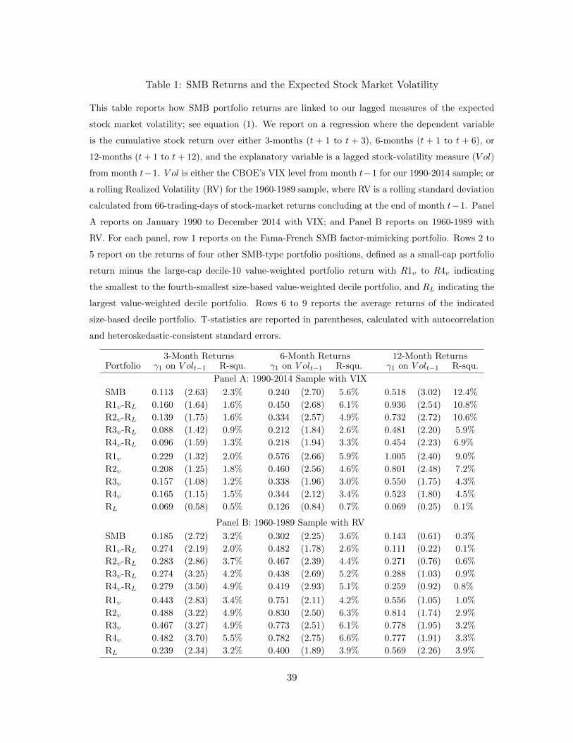
Table 1: SMB Returns and the Expected Stock Market Volatility

This table reports how SMB portfolio returns are linked to our lagged measures of the expected

stock market volatility; see equation (1). We report on a regression where the dependent variable

is the cumulative stock return over either 3-months (t + 1 to t + 3), 6-months (t + 1 to t + 6), or

12-months (t+ 1 to t+ 12), and the explanatory variable is a lagged stock-volatility measure (V ol)

from month t−1. V ol is either the CBOE’s VIX level from month t−1 for our 1990-2014 sample; or

a rolling Realized Volatility (RV) for the 1960-1989 sample, where RV is a rolling standard deviation

calculated from 66-trading-days of stock-market returns concluding at the end of month t−1. Panel

A reports on January 1990 to December 2014 with VIX; and Panel B reports on 1960-1989 with

RV. For each panel, row 1 reports on the Fama-French SMB factor-mimicking portfolio. Rows 2 to

5 report on the returns of four other SMB-type portfolio positions, defined as a small-cap portfolio

return minus the large-cap decile-10 value-weighted portfolio return with R1v to R4v indicating

the smallest to the fourth-smallest size-based value-weighted decile portfolio, and RL indicating the

largest value-weighted decile portfolio. Rows 6 to 9 reports the average returns of the indicated

size-based decile portfolio. T-statistics are reported in parentheses, calculated with autocorrelation

and heteroskedastic-consistent standard errors.

3-Month Returns 6-Month Returns 12-Month ReturnsPortfolio γ1 on V olt−1 R-squ. γ1 on V olt−1 R-squ. γ1 on V olt−1 R-squ.

Panel A: 1990-2014 Sample with VIX

SMB 0.113 (2.63) 2.3% 0.240 (2.70) 5.6% 0.518 (3.02) 12.4%

R1v-RL 0.160 (1.64) 1.6% 0.450 (2.68) 6.1% 0.936 (2.54) 10.8%

R2v-RL 0.139 (1.75) 1.6% 0.334 (2.57) 4.9% 0.732 (2.72) 10.6%

R3v-RL 0.088 (1.42) 0.9% 0.212 (1.84) 2.6% 0.481 (2.20) 5.9%

R4v-RL 0.096 (1.59) 1.3% 0.218 (1.94) 3.3% 0.454 (2.23) 6.9%

R1v 0.229 (1.32) 2.0% 0.576 (2.66) 5.9% 1.005 (2.40) 9.0%

R2v 0.208 (1.25) 1.8% 0.460 (2.56) 4.6% 0.801 (2.48) 7.2%

R3v 0.157 (1.08) 1.2% 0.338 (1.96) 3.0% 0.550 (1.75) 4.3%

R4v 0.165 (1.15) 1.5% 0.344 (2.12) 3.4% 0.523 (1.80) 4.5%

RL 0.069 (0.58) 0.5% 0.126 (0.84) 0.7% 0.069 (0.25) 0.1%

Panel B: 1960-1989 Sample with RV

SMB 0.185 (2.72) 3.2% 0.302 (2.25) 3.6% 0.143 (0.61) 0.3%

R1v-RL 0.274 (2.19) 2.0% 0.482 (1.78) 2.6% 0.111 (0.22) 0.1%

R2v-RL 0.283 (2.86) 3.7% 0.467 (2.39) 4.4% 0.271 (0.76) 0.6%

R3v-RL 0.274 (3.25) 4.2% 0.438 (2.69) 5.2% 0.288 (1.03) 0.9%

R4v-RL 0.279 (3.50) 4.9% 0.419 (2.93) 5.1% 0.259 (0.92) 0.8%

R1v 0.443 (2.83) 3.4% 0.751 (2.11) 4.2% 0.556 (1.05) 1.0%

R2v 0.488 (3.22) 4.9% 0.830 (2.50) 6.3% 0.814 (1.74) 2.9%

R3v 0.467 (3.27) 4.9% 0.773 (2.51) 6.1% 0.778 (1.95) 3.2%

R4v 0.482 (3.70) 5.5% 0.782 (2.75) 6.6% 0.777 (1.91) 3.3%

RL 0.239 (2.34) 3.2% 0.400 (1.89) 3.9% 0.569 (2.26) 3.9%

39

Table 2: SMB Average Returns, following Each Decile of the Exp. Stock Volatility

This table reports on conditional average SMB-type returns for decile subsets, where the deciles

refer to the decile of the lagged volatility measure. Panels A to C report on 3-, 6-, and 12-month

average cumulative returns in percentage units, respectively, per equation (2). For each panel, Row

1 reports on the Fama-French SMB portfolio. Rows 2 to 5 report on the returns of four other

SMB-type portfolio positions, as defined in Table 1. Rows 6 to 9 report the average returns of the

indicated size-based decile portfolio. The ‘All’ column reports on the overall unconditional average

return. The ten decile columns report on conditional subset average returns for each portfolio with

the cumulative return starting in month t+1, based on the decile classification of our stock-volatility

measures ending in month t− 1. The stock-volatility measure is the VIX for our 1990-2014 sample,

and our rolling RV for our 1960-1989 sample. P-values are indicated by the superscript for a null

that the average return is zero, based on autocorrelation and heteroskedastic-consistent standard

errors, with 1 (2) [3] indicating a 1% (5%) [10%] p-value.

All Dc 1 Dc 2 Dc 3 Dc 4 Dc 5 Dc 6 Dc 7 Dc 8 Dc 9 Dc 10

γ1 γ2 γ3 γ4 γ5 γ6 γ7 γ8 γ9 γ10

Panel A.1: 3-months Returns, 1990-2014 Sample with VIX Deciles

SMB 0.60 0.18 0.65 -0.06 -0.13 -1.572 -0.45 1.16 0.60 2.13 3.281

R1v-RL 1.04 0.26 1.41 -0.51 0.80 -2.751 0.30 2.71 0.44 2.43 5.122

R2v-RL 0.78 0.02 0.99 -0.01 0.11 -2.821 -0.90 1.78 1.31 2.86 4.212

R3v-RL 0.88 0.41 2.122 0.34 0.55 -1.51 -1.19 0.98 0.55 2.52 3.841

R4v-RL 0.53 -0.34 1.493 0.13 0.10 -2.012 -0.85 0.76 0.48 1.69 3.741

R1v 3.611 3.142 4.871 3.223 3.50 -2.10 1.19 2.34 2.41 5.941 11.481

R2v 3.351 2.912 4.452 3.732 2.81 -2.17 0.00 1.42 3.28 6.371 10.581

R3v 3.451 3.292 5.581 4.081 3.25 -0.86 -0.29 0.62 2.51 6.031 10.201

R4v 3.101 2.552 4.951 3.861 2.79 -1.36 0.05 0.40 2.45 5.201 10.111

RL 2.571 2.881 3.461 3.731 2.702 0.65 0.90 -0.36 1.97 3.511 6.372

Panel A.2: 3-month Returns, 1960-1989 Sample with RV Deciles

SMB 0.823 1.06 -0.50 0.60 0.96 0.96 -1.12 0.48 -1.18 3.252 3.681

R1v-RL 1.24 2.40 -0.41 1.64 1.05 0.90 -2.14 0.68 -1.92 5.652 4.572

R2v-RL 0.99 1.19 -0.08 1.07 0.71 0.61 -1.69 0.33 -1.49 4.692 4.572

R3v-RL 1.282 1.66 -0.17 0.84 1.21 0.74 -0.99 0.98 -0.65 4.911 4.321

R4v-RL 1.172 1.06 -0.05 0.66 1.33 1.35 -1.25 0.94 -0.99 4.312 4.381

R1v 3.841 2.62 -0.17 3.04 5.581 2.94 0.90 4.543 0.74 6.982 11.291

R2v 3.591 1.41 0.16 2.47 5.251 2.65 1.35 4.193 1.18 6.022 11.291

R3v 3.881 1.88 0.06 2.24 5.741 2.79 2.04 4.842 2.02 6.232 11.031

R4v 3.771 1.27 0.19 2.06 5.871 3.393 1.79 4.802 1.68 5.642 11.091

RL 2.601 0.22 0.24 1.39 4.541 2.043 3.043 3.861 2.67 1.33 6.721

40

Table 2: (continued)

All Dc 1 Dc 2 Dc 3 Dc 4 Dc 5 Dc 6 Dc 7 Dc 8 Dc 9 Dc 10

γ1 γ2 γ3 γ4 γ5 γ6 γ7 γ8 γ9 γ10Panel B.1: 6-month Returns, 1990-2014 Sample with VIX Deciles

SMB 1.09 -0.31 1.42 -0.54 -0.76 -2.242 -1.52 1.53 1.06 4.791 6.971

R1v-RL 2.10 -0.01 2.76 -0.41 -0.28 -4.562 -0.68 1.80 1.60 6.401 13.591

R2v-RL 1.39 -0.56 1.89 -0.94 -0.91 -4.021 -2.40 1.79 2.49 6.681 9.201

R3v-RL 1.59 0.18 3.442 0.27 0.61 -1.73 -2.45 0.96 0.90 4.881 8.281

R4v-RL 0.93 -1.21 2.441 -0.39 -0.16 -2.70 -2.07 1.34 0.39 3.772 7.511

R1v 7.353 6.943 8.763 6.952 6.912 -1.88 4.09 2.01 2.24 10.331 26.351

R2v 6.643 6.383 7.883 6.422 6.293 -1.34 2.37 2.00 3.13 10.611 21.951

R3v 6.843 7.133 9.433 7.623 7.813 0.95 2.32 1.16 1.54 8.801 21.031

R4v 6.183 5.733 8.433 6.973 7.043 -0.02 2.70 1.54 1.03 7.691 20.261

RL 5.253 6.953 6.003 7.363 7.203 2.68 4.772 0.20 0.64 3.92 12.761

Panel B.2: 6-month Returns, 1960-1989 Sample with RV Deciles

SMB 1.743 1.69 -1.90 1.04 2.11 2.62 0.45 1.83 -1.13 3.913 6.791

R1v-RL 2.75 3.46 -1.67 3.06 3.40 3.32 -0.74 1.50 -1.96 7.143 9.951

R2v-RL 2.15 1.28 -1.52 1.74 2.28 2.45 -0.07 1.25 -1.21 6.192 9.101

R3v-RL 2.682 2.45 -1.58 1.68 2.66 2.85 1.37 2.37 0.30 6.332 8.351

R4v-RL 2.482 1.80 -1.70 0.71 2.89 3.813 0.95 3.093 -0.33 5.912 7.711

R1v 8.111 5.29 -0.04 6.72 10.731 6.713 6.02 8.951 6.16 8.04 22.371

R2v 7.521 3.11 0.11 5.40 9.611 5.842 6.69 8.691 6.913 7.09 21.531

R3v 8.041 4.28 0.05 5.34 9.991 6.242 8.123 9.821 8.422 7.23 20.781

R4v 7.841 3.63 -0.07 4.37 10.221 7.201 7.703 10.541 7.792 6.80 20.131

RL 5.361 1.83 1.63 3.663 7.331 3.382 6.751 7.451 8.122 0.90 12.431

Panel C.1: 12-Month Returns, 1990-2014 with VIX Deciles

SMB 2.32 -2.45 1.47 -1.48 -0.27 -1.08 -0.97 1.90 1.00 11.211 12.641

R1v-RL 4.48 -3.94 3.39 -1.85 1.43 -1.88 -0.79 3.42 0.50 17.972 24.541

R2v-RL 2.98 -4.373 1.56 -3.12 -0.67 -2.40 -2.08 2.96 3.75 15.971 16.481

R3v-RL 3.19 -2.64 4.30 0.00 3.22 0.08 -1.11 0.12 2.10 10.571 14.261

R4v-RL 1.78 -4.561 1.63 -1.59 1.24 -0.57 -1.27 0.38 1.24 8.271 12.051

R1v 15.521 10.243 16.481 14.151 15.301 8.723 12.261 8.86 2.44 21.372 44.721

R2v 14.021 9.823 14.651 12.881 13.201 8.19 10.961 8.40 5.70 19.362 36.671

R3v 14.231 11.552 17.391 16.001 17.091 10.682 11.931 5.56 4.05 13.972 34.441

R4v 12.821 9.622 14.721 14.411 15.111 10.022 11.771 5.82 3.18 11.673 32.231

RL 11.031 14.181 13.091 16.001 13.881 10.602 13.041 5.44 1.94 3.40 20.181

Panel C.2: 12-Month Returns, 1960-1989 with RV Deciles

SMB 3.80 6.35 -1.24 2.76 5.98 3.01 3.62 0.45 2.50 7.493 7.601

R1v-RL 6.13 12.953 0.92 7.07 10.15 2.94 4.06 -1.19 2.57 11.31 11.332

R2v-RL 4.76 6.50 0.58 3.94 7.10 2.67 4.01 -1.34 3.17 10.123 11.371

R3v-RL 5.682 9.252 0.56 4.42 7.273 4.20 5.26 0.77 4.69 9.472 11.251

R4v-RL 5.282 8.76 -0.53 2.36 7.172 4.65 4.77 1.80 3.94 9.862 10.431

R1v 16.971 19.841 7.39 11.86 20.061 13.251 19.312 11.482 18.642 17.503 30.631

R2v 15.591 13.391 7.06 8.72 17.001 12.981 19.262 11.341 19.242 16.313 30.671

R3v 16.521 16.131 7.03 9.21 17.181 14.521 20.501 13.451 20.751 15.652 30.551

R4v 16.111 15.641 5.94 7.15 17.071 14.971 20.021 14.481 20.011 16.042 29.731

RL 10.831 6.892 6.473 4.79 9.901 10.321 15.251 12.681 16.071 6.19 19.301

41

Table 3: SMB Average Returns Following a Top-Quintile Expected Volatility

This table reports how average SMB portfolio returns are different following top-quintile observations

of our stock-volatility measures; see equation (3). For each panel, rows 1 to 5 report on the average

of the return differences for five different small-minus-large-cap long-short portfolios, and rows 6 to

9 report on the average returns for the denoted size-based decile portfolios; as defined in Table 1.

Panels A through C report on average 3-month returns (over t+ 1 to t+ 3), 6-month returns (over

t + 1 to t + 6), and 12-month returns (over t + 1 to t + 12), respectively. For each panel, column

two denotes the average return for periods when the lagged volatility measures (V olt−1) was >= its

80th percentile as the base intercept case ψ0; column three indicates the difference in average returns

following months where the V olt−1 level was < its 80th percentile with the ψ1 coefficient on the

conditional dummy variable, as compared to the average return for the base high-Vol case. Column

four indicates the simple average return following the relatively lower V ol condition (=ψ0 + ψ1).

The final column gives the regression’s R-squared value. We report separate results for our 1990-

2014 sample period conditional on VIX, and our 1960-1989 sample period conditional on our 66-

trading-day rolling RV. T-statistics are reported in parentheses, calculated with autocorrelation and

heteroskedastic-consistent standard errors.

1. Portfolio 2. ψ0 Intercept 3. ψ1 Dummy 4. ψ0 + ψ1 5. R-Squ.

Average if Diff. Av. if Average if

Vol>= 80th Pctl Vol< 80th Pctl Vol< 80th Pctl

Panel A.1: 3-months Returns, 1990-2014, with VIX as Vol

SMB 2.71 (3.01) -2.67 (-2.83) 0.05 (0.10) 3.5%

R1v-RL 3.79 (2.19) -3.47 (-2.01) 0.33 (0.39) 2.1%

R2v-RL 3.55 (2.49) -3.49 (-2.40) 0.06 (0.08) 2.8%

R3v-RL 3.19 (2.72) -2.91 (-2.38) 0.28 (0.23) 2.8%

R4v-RL 2.73 (2.36) -2.76 (-2.33) -0.03 (-0.06) 3.0%

R1v 8.76 (3.97) -6.45 (-2.85) 2.31 (2.01) 4.4%

R2v 8.51 (4.18) -6.47 (-3.04) 2.04 (1.91) 4.8%

R3v 8.15 (4.54) -5.90 (-3.09) 2.26 (2.27) 4.8%

R4v 7.69 (4.31) -5.75 (-3.06) 1.95 (2.10) 5.0%

RL 4.96 (3.21) -2.98 (-1.92) 1.98 (2.89) 2.6%

Panel A.2: 3-months Returns, 1960-1989, with RV as Vol

SMB 3.44 (3.40) -3.28 (-2.94) 0.15 (0.30) 5.4%

R1v-RL 5.01 (3.24) -4.73 (-2.68) 0.27 (0.31) 4.1%

R2v-RL 4.54 (3.28) -4.46 (-2.90) 0.09 (0.12) 5.2%

R3v-RL 4.51 (3.74) -4.05 (-3.01) 0.46 (0.75) 5.4%

R4v-RL 4.28 (3.52) -3.90 (-2.90) 0.38 (0.65) 5.4%

R1v 9.01 (3.76) -6.45 (-2.55) 2.56 (2.26) 3.9%

R2v 8.55 (3.68) -6.18 (-2.57) 2.37 (2.39) 4.2%

R3v 8.51 (3.93) -5.77 (-2.56) 2.74 (2.91) 4.0%

R4v 8.29 (3.95) -5.62 (-2.57) 2.67 (2.89) 4.0%

RL 4.00 (3.04) -1.72 (-1.27) 2.28 (3.73) 0.9%

42

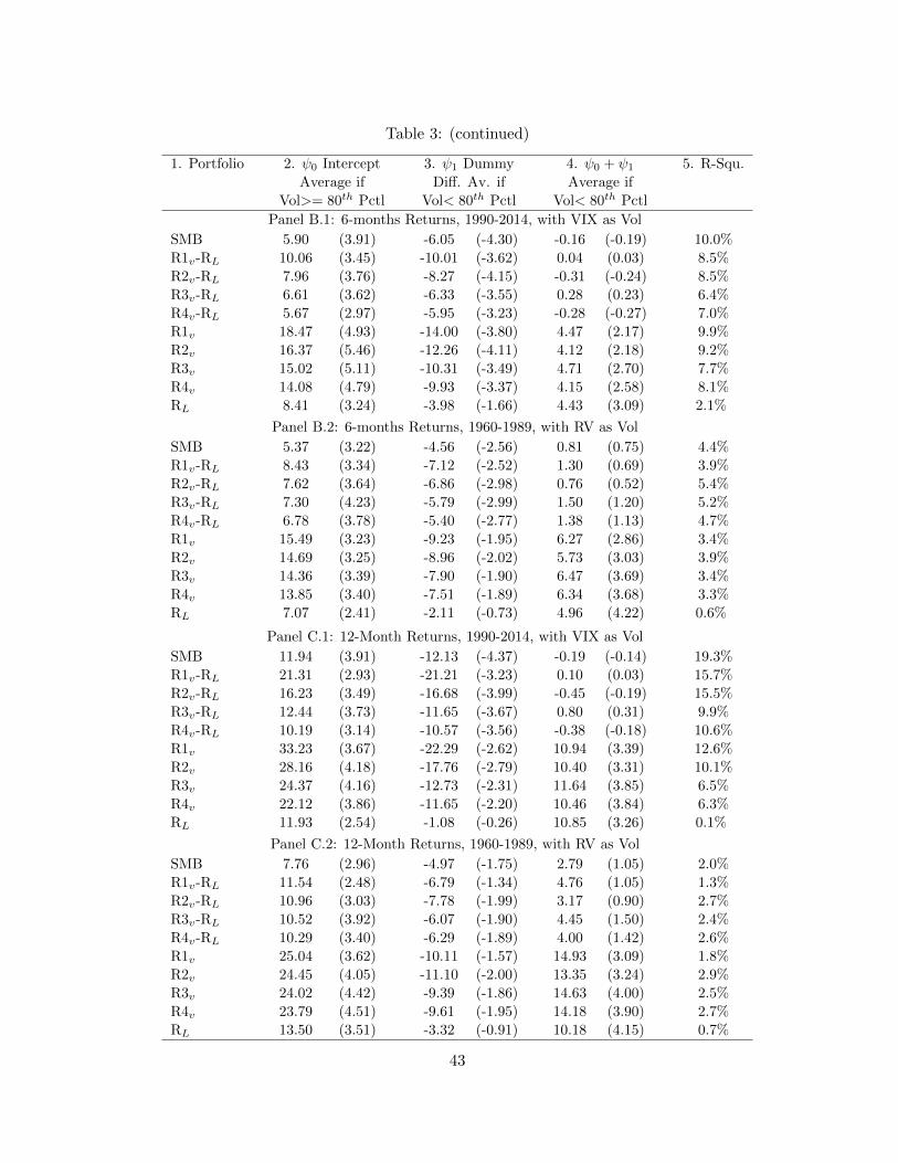
Table 3: (continued)

1. Portfolio 2. ψ0 Intercept 3. ψ1 Dummy 4. ψ0 + ψ1 5. R-Squ.

Average if Diff. Av. if Average if

Vol>= 80th Pctl Vol< 80th Pctl Vol< 80th Pctl

Panel B.1: 6-months Returns, 1990-2014, with VIX as Vol

SMB 5.90 (3.91) -6.05 (-4.30) -0.16 (-0.19) 10.0%

R1v-RL 10.06 (3.45) -10.01 (-3.62) 0.04 (0.03) 8.5%

R2v-RL 7.96 (3.76) -8.27 (-4.15) -0.31 (-0.24) 8.5%

R3v-RL 6.61 (3.62) -6.33 (-3.55) 0.28 (0.23) 6.4%

R4v-RL 5.67 (2.97) -5.95 (-3.23) -0.28 (-0.27) 7.0%

R1v 18.47 (4.93) -14.00 (-3.80) 4.47 (2.17) 9.9%

R2v 16.37 (5.46) -12.26 (-4.11) 4.12 (2.18) 9.2%

R3v 15.02 (5.11) -10.31 (-3.49) 4.71 (2.70) 7.7%

R4v 14.08 (4.79) -9.93 (-3.37) 4.15 (2.58) 8.1%

RL 8.41 (3.24) -3.98 (-1.66) 4.43 (3.09) 2.1%

Panel B.2: 6-months Returns, 1960-1989, with RV as Vol

SMB 5.37 (3.22) -4.56 (-2.56) 0.81 (0.75) 4.4%

R1v-RL 8.43 (3.34) -7.12 (-2.52) 1.30 (0.69) 3.9%

R2v-RL 7.62 (3.64) -6.86 (-2.98) 0.76 (0.52) 5.4%

R3v-RL 7.30 (4.23) -5.79 (-2.99) 1.50 (1.20) 5.2%

R4v-RL 6.78 (3.78) -5.40 (-2.77) 1.38 (1.13) 4.7%

R1v 15.49 (3.23) -9.23 (-1.95) 6.27 (2.86) 3.4%

R2v 14.69 (3.25) -8.96 (-2.02) 5.73 (3.03) 3.9%

R3v 14.36 (3.39) -7.90 (-1.90) 6.47 (3.69) 3.4%

R4v 13.85 (3.40) -7.51 (-1.89) 6.34 (3.68) 3.3%

RL 7.07 (2.41) -2.11 (-0.73) 4.96 (4.22) 0.6%

Panel C.1: 12-Month Returns, 1990-2014, with VIX as Vol

SMB 11.94 (3.91) -12.13 (-4.37) -0.19 (-0.14) 19.3%

R1v-RL 21.31 (2.93) -21.21 (-3.23) 0.10 (0.03) 15.7%

R2v-RL 16.23 (3.49) -16.68 (-3.99) -0.45 (-0.19) 15.5%

R3v-RL 12.44 (3.73) -11.65 (-3.67) 0.80 (0.31) 9.9%

R4v-RL 10.19 (3.14) -10.57 (-3.56) -0.38 (-0.18) 10.6%

R1v 33.23 (3.67) -22.29 (-2.62) 10.94 (3.39) 12.6%

R2v 28.16 (4.18) -17.76 (-2.79) 10.40 (3.31) 10.1%

R3v 24.37 (4.16) -12.73 (-2.31) 11.64 (3.85) 6.5%

R4v 22.12 (3.86) -11.65 (-2.20) 10.46 (3.84) 6.3%

RL 11.93 (2.54) -1.08 (-0.26) 10.85 (3.26) 0.1%

Panel C.2: 12-Month Returns, 1960-1989, with RV as Vol

SMB 7.76 (2.96) -4.97 (-1.75) 2.79 (1.05) 2.0%

R1v-RL 11.54 (2.48) -6.79 (-1.34) 4.76 (1.05) 1.3%

R2v-RL 10.96 (3.03) -7.78 (-1.99) 3.17 (0.90) 2.7%

R3v-RL 10.52 (3.92) -6.07 (-1.90) 4.45 (1.50) 2.4%

R4v-RL 10.29 (3.40) -6.29 (-1.89) 4.00 (1.42) 2.6%

R1v 25.04 (3.62) -10.11 (-1.57) 14.93 (3.09) 1.8%

R2v 24.45 (4.05) -11.10 (-2.00) 13.35 (3.24) 2.9%

R3v 24.02 (4.42) -9.39 (-1.86) 14.63 (4.00) 2.5%

R4v 23.79 (4.51) -9.61 (-1.95) 14.18 (3.90) 2.7%

RL 13.50 (3.51) -3.32 (-0.91) 10.18 (4.15) 0.7%

43

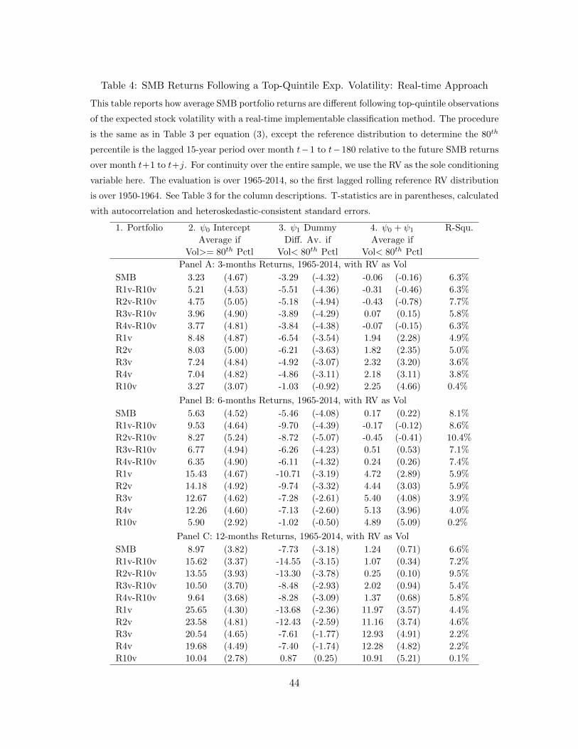
Table 4: SMB Returns Following a Top-Quintile Exp. Volatility: Real-time Approach

This table reports how average SMB portfolio returns are different following top-quintile observations

of the expected stock volatility with a real-time implementable classification method. The procedure

is the same as in Table 3 per equation (3), except the reference distribution to determine the 80th

percentile is the lagged 15-year period over month t−1 to t−180 relative to the future SMB returns

over month t+1 to t+j. For continuity over the entire sample, we use the RV as the sole conditioning

variable here. The evaluation is over 1965-2014, so the first lagged rolling reference RV distribution

is over 1950-1964. See Table 3 for the column descriptions. T-statistics are in parentheses, calculated

with autocorrelation and heteroskedastic-consistent standard errors.

1. Portfolio 2. ψ0 Intercept 3. ψ1 Dummy 4. ψ0 + ψ1 R-Squ.

Average if Diff. Av. if Average if

Vol>= 80th Pctl Vol< 80th Pctl Vol< 80th Pctl

Panel A: 3-months Returns, 1965-2014, with RV as Vol

SMB 3.23 (4.67) -3.29 (-4.32) -0.06 (-0.16) 6.3%

R1v-R10v 5.21 (4.53) -5.51 (-4.36) -0.31 (-0.46) 6.3%

R2v-R10v 4.75 (5.05) -5.18 (-4.94) -0.43 (-0.78) 7.7%

R3v-R10v 3.96 (4.90) -3.89 (-4.29) 0.07 (0.15) 5.8%

R4v-R10v 3.77 (4.81) -3.84 (-4.38) -0.07 (-0.15) 6.3%

R1v 8.48 (4.87) -6.54 (-3.54) 1.94 (2.28) 4.9%

R2v 8.03 (5.00) -6.21 (-3.63) 1.82 (2.35) 5.0%

R3v 7.24 (4.84) -4.92 (-3.07) 2.32 (3.20) 3.6%

R4v 7.04 (4.82) -4.86 (-3.11) 2.18 (3.11) 3.8%

R10v 3.27 (3.07) -1.03 (-0.92) 2.25 (4.66) 0.4%

Panel B: 6-months Returns, 1965-2014, with RV as Vol

SMB 5.63 (4.52) -5.46 (-4.08) 0.17 (0.22) 8.1%

R1v-R10v 9.53 (4.64) -9.70 (-4.39) -0.17 (-0.12) 8.6%

R2v-R10v 8.27 (5.24) -8.72 (-5.07) -0.45 (-0.41) 10.4%

R3v-R10v 6.77 (4.94) -6.26 (-4.23) 0.51 (0.53) 7.1%

R4v-R10v 6.35 (4.90) -6.11 (-4.32) 0.24 (0.26) 7.4%

R1v 15.43 (4.67) -10.71 (-3.19) 4.72 (2.89) 5.9%

R2v 14.18 (4.92) -9.74 (-3.32) 4.44 (3.03) 5.9%

R3v 12.67 (4.62) -7.28 (-2.61) 5.40 (4.08) 3.9%

R4v 12.26 (4.60) -7.13 (-2.60) 5.13 (3.96) 4.0%

R10v 5.90 (2.92) -1.02 (-0.50) 4.89 (5.09) 0.2%

Panel C: 12-months Returns, 1965-2014, with RV as Vol

SMB 8.97 (3.82) -7.73 (-3.18) 1.24 (0.71) 6.6%

R1v-R10v 15.62 (3.37) -14.55 (-3.15) 1.07 (0.34) 7.2%

R2v-R10v 13.55 (3.93) -13.30 (-3.78) 0.25 (0.10) 9.5%

R3v-R10v 10.50 (3.70) -8.48 (-2.93) 2.02 (0.94) 5.4%

R4v-R10v 9.64 (3.68) -8.28 (-3.09) 1.37 (0.68) 5.8%

R1v 25.65 (4.30) -13.68 (-2.36) 11.97 (3.57) 4.4%

R2v 23.58 (4.81) -12.43 (-2.59) 11.16 (3.74) 4.6%

R3v 20.54 (4.65) -7.61 (-1.77) 12.93 (4.91) 2.2%

R4v 19.68 (4.49) -7.40 (-1.74) 12.28 (4.82) 2.2%

R10v 10.04 (2.78) 0.87 (0.25) 10.91 (5.21) 0.1%

44

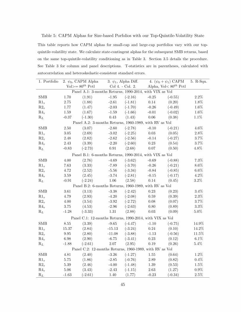
Table 5: CAPM Alphas for Size-based Porfolios with our Top-Quintile-Volatility State

This table reports how CAPM alphas for small-cap and large-cap portfolios vary with our top-

quintile-volatility state. We calculate state-contingent alphas for the subsequent SMB returns, based

on the same top-quintile-volatility conditioning as in Table 3. Section 3.5 details the procedure.

See Table 3 for column and panel descriptions. T-statistics are in parentheses, calculated with

autocorrelation and heteroskedastic-consistent standard errors.

1. Portfolio 2. ψ0, CAPM Alpha 3. ψ1, Alpha Diff. 4. (ψ0 + ψ1) CAPM 5. R-Squ.

Vol>= 80th Pctl Col 4. - Col. 2. Alpha, Vol< 80th Pctl

Panel A.1: 3-months Returns, 1990-2014, with VIX as Vol

SMB 1.70 (1.91) -1.95 (-2.16) -0.25 (-0.55) 2.2%

R1v 2.75 (1.88) -2.61 (-1.81) 0.14 (0.20) 1.8%

R2v 1.77 (1.47) -2.03 (-1.70) -0.26 (-0.49) 1.6%

R4v 1.59 (1.67) -1.59 (-1.66) -0.01 (-0.02) 1.6%

RL -0.37 (-1.30) 0.43 (1.43) 0.06 (0.38) 1.1%

Panel A.2: 3-months Returns, 1960-1989, with RV as Vol

SMB 2.50 (3.07) -2.60 (-2.78) -0.10 (-0.21) 4.6%

R1v 3.05 (2.69) -3.02 (-2.25) 0.03 (0.05) 2.8%

R2v 2.48 (2.82) -2.62 (-2.56) -0.14 (-0.27) 3.7%

R4v 2.43 (3.39) -2.20 (-2.60) 0.23 (0.54) 3.7%

RL -0.83 (-2.73) 0.91 (2.68) 0.07 (0.50) 4.8%

Panel B.1: 6-months Returns, 1990-2014, with VIX as Vol

SMB 4.00 (2.76) -4.69 (-3.62) -0.69 (-0.88) 7.3%

R1v 7.63 (3.33) -7.89 (-3.70) -0.26 (-0.21) 8.6%

R2v 4.72 (2.52) -5.56 (-3.34) -0.84 (-0.85) 6.6%

R4v 3.59 (2.45) -3.74 (-2.81) -0.15 (-0.17) 4.2%

RL -0.91 (-2.24) 1.06 (2.58) 0.14 (0.45) 3.2%

Panel B.2: 6-months Returns, 1960-1989, with RV as Vol

SMB 3.61 (3.13) -3.38 (-2.42) 0.23 (0.23) 3.4%

R1v 4.79 (2.93) -4.20 (-2.08) 0.59 (0.39) 2.3%

R2v 4.00 (3.54) -3.92 (-2.72) 0.08 (0.07) 3.7%

R4v 3.75 (4.53) -2.96 (-2.63) 0.80 (0.89) 3.3%

RL -1.28 (-3.33) 1.31 (2.88) 0.03 (0.09) 5.0%

Panel C.1: 12-months Returns, 1990-2014, with VIX as Vol

SMB 8.55 (3.39) -9.65 (-4.47) -1.10 (-0.75) 14.9%

R1v 15.37 (2.84) -15.13 (-3.24) 0.24 (0.10) 14.2%

R2v 9.95 (2.80) -11.08 (-3.88) -1.13 (-0.56) 11.5%

R4v 6.98 (2.90) -6.75 (-3.41) 0.23 (0.12) 6.1%

RL -1.88 (-2.61) 2.07 (2.95) 0.19 (0.26) 5.4%

Panel C.2: 12-months Returns, 1960-1989, with RV as Vol

SMB 4.81 (2.40) -3.26 (-1.27) 1.55 (0.64) 1.2%

R1v 5.75 (1.86) -2.85 (-0.76) 2.89 (0.82) 0.4%

R2v 5.39 (2.46) -4.00 (-1.48) 1.39 (0.53) 1.5%

R4v 5.06 (3.43) -2.43 (-1.15) 2.63 (1.27) 0.9%

RL -1.63 (-2.61) 1.40 (1.77) -0.23 (-0.34) 2.5%

45

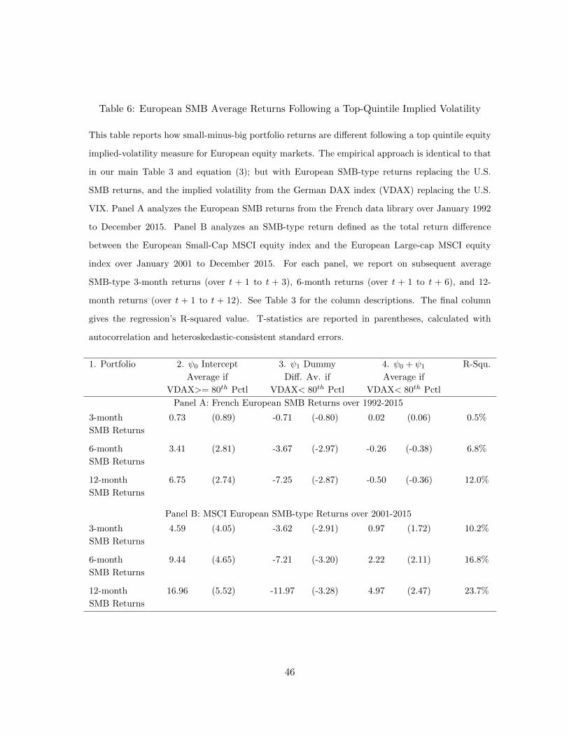
Table 6: European SMB Average Returns Following a Top-Quintile Implied Volatility

This table reports how small-minus-big portfolio returns are different following a top quintile equity

implied-volatility measure for European equity markets. The empirical approach is identical to that

in our main Table 3 and equation (3); but with European SMB-type returns replacing the U.S.

SMB returns, and the implied volatility from the German DAX index (VDAX) replacing the U.S.

VIX. Panel A analyzes the European SMB returns from the French data library over January 1992

to December 2015. Panel B analyzes an SMB-type return defined as the total return difference

between the European Small-Cap MSCI equity index and the European Large-cap MSCI equity

index over January 2001 to December 2015. For each panel, we report on subsequent average

SMB-type 3-month returns (over t + 1 to t + 3), 6-month returns (over t + 1 to t + 6), and 12-

month returns (over t + 1 to t + 12). See Table 3 for the column descriptions. The final column

gives the regression’s R-squared value. T-statistics are reported in parentheses, calculated with

autocorrelation and heteroskedastic-consistent standard errors.

1. Portfolio 2. ψ0 Intercept 3. ψ1 Dummy 4. ψ0 + ψ1 R-Squ.

Average if Diff. Av. if Average if

VDAX>= 80th Pctl VDAX< 80th Pctl VDAX< 80th Pctl

Panel A: French European SMB Returns over 1992-2015

3-month 0.73 (0.89) -0.71 (-0.80) 0.02 (0.06) 0.5%

SMB Returns

6-month 3.41 (2.81) -3.67 (-2.97) -0.26 (-0.38) 6.8%

SMB Returns

12-month 6.75 (2.74) -7.25 (-2.87) -0.50 (-0.36) 12.0%

SMB Returns

Panel B: MSCI European SMB-type Returns over 2001-2015

3-month 4.59 (4.05) -3.62 (-2.91) 0.97 (1.72) 10.2%

SMB Returns

6-month 9.44 (4.65) -7.21 (-3.20) 2.22 (2.11) 16.8%

SMB Returns

12-month 16.96 (5.52) -11.97 (-3.28) 4.97 (2.47) 23.7%

SMB Returns

46

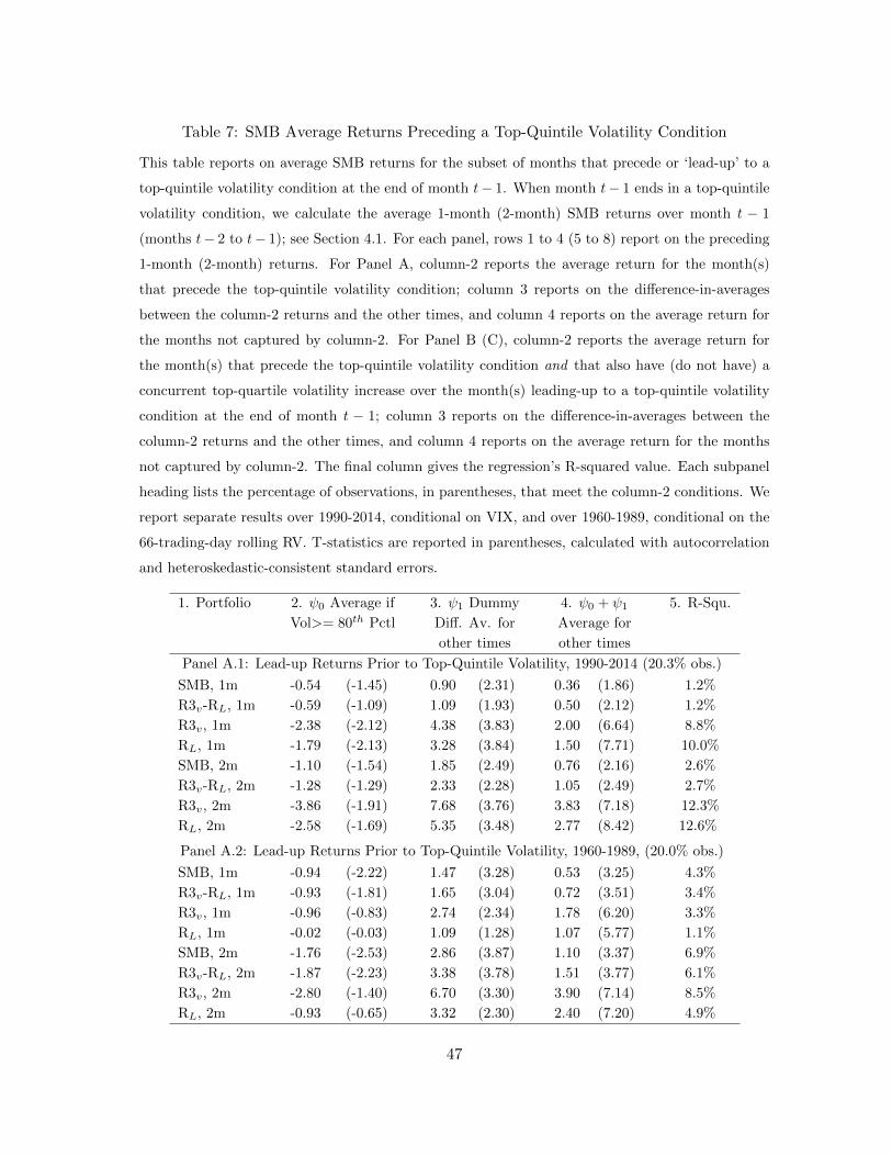
Table 7: SMB Average Returns Preceding a Top-Quintile Volatility Condition

This table reports on average SMB returns for the subset of months that precede or ‘lead-up’ to a

top-quintile volatility condition at the end of month t− 1. When month t− 1 ends in a top-quintile

volatility condition, we calculate the average 1-month (2-month) SMB returns over month t − 1

(months t− 2 to t− 1); see Section 4.1. For each panel, rows 1 to 4 (5 to 8) report on the preceding

1-month (2-month) returns. For Panel A, column-2 reports the average return for the month(s)

that precede the top-quintile volatility condition; column 3 reports on the difference-in-averages

between the column-2 returns and the other times, and column 4 reports on the average return for

the months not captured by column-2. For Panel B (C), column-2 reports the average return for

the month(s) that precede the top-quintile volatility condition and that also have (do not have) a

concurrent top-quartile volatility increase over the month(s) leading-up to a top-quintile volatility

condition at the end of month t − 1; column 3 reports on the difference-in-averages between the

column-2 returns and the other times, and column 4 reports on the average return for the months

not captured by column-2. The final column gives the regression’s R-squared value. Each subpanel

heading lists the percentage of observations, in parentheses, that meet the column-2 conditions. We

report separate results over 1990-2014, conditional on VIX, and over 1960-1989, conditional on the

66-trading-day rolling RV. T-statistics are reported in parentheses, calculated with autocorrelation

and heteroskedastic-consistent standard errors.

1. Portfolio 2. ψ0 Average if 3. ψ1 Dummy 4. ψ0 + ψ1 5. R-Squ.

Vol>= 80th Pctl Diff. Av. for Average for

other times other times

Panel A.1: Lead-up Returns Prior to Top-Quintile Volatility, 1990-2014 (20.3% obs.)

SMB, 1m -0.54 (-1.45) 0.90 (2.31) 0.36 (1.86) 1.2%

R3v-RL, 1m -0.59 (-1.09) 1.09 (1.93) 0.50 (2.12) 1.2%

R3v, 1m -2.38 (-2.12) 4.38 (3.83) 2.00 (6.64) 8.8%

RL, 1m -1.79 (-2.13) 3.28 (3.84) 1.50 (7.71) 10.0%

SMB, 2m -1.10 (-1.54) 1.85 (2.49) 0.76 (2.16) 2.6%

R3v-RL, 2m -1.28 (-1.29) 2.33 (2.28) 1.05 (2.49) 2.7%

R3v, 2m -3.86 (-1.91) 7.68 (3.76) 3.83 (7.18) 12.3%

RL, 2m -2.58 (-1.69) 5.35 (3.48) 2.77 (8.42) 12.6%

Panel A.2: Lead-up Returns Prior to Top-Quintile Volatility, 1960-1989, (20.0% obs.)

SMB, 1m -0.94 (-2.22) 1.47 (3.28) 0.53 (3.25) 4.3%

R3v-RL, 1m -0.93 (-1.81) 1.65 (3.04) 0.72 (3.51) 3.4%

R3v, 1m -0.96 (-0.83) 2.74 (2.34) 1.78 (6.20) 3.3%

RL, 1m -0.02 (-0.03) 1.09 (1.28) 1.07 (5.77) 1.1%

SMB, 2m -1.76 (-2.53) 2.86 (3.87) 1.10 (3.37) 6.9%

R3v-RL, 2m -1.87 (-2.23) 3.38 (3.78) 1.51 (3.77) 6.1%

R3v, 2m -2.80 (-1.40) 6.70 (3.30) 3.90 (7.14) 8.5%

RL, 2m -0.93 (-0.65) 3.32 (2.30) 2.40 (7.20) 4.9%

47

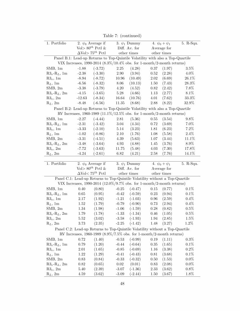
Table 7: (continued)

1. Portfolio 2. ψ0 Average if 3. ψ1 Dummy 4. ψ0 + ψ1 5. R-Squ.

Vol> 80th Pctl & Diff. Av. for Average for

∆Vol> 75th Pctl other times other times

Panel B.1: Lead-up Returns to Top-Quintile Volatility with also a Top-Quartile

VIX Increases, 1990-2014 (8.3%/10.4% obs. for 1-month/2-month returns)

SMB, 1m -1.88 (-3.72) 2.25 (4.28) 0.37 (1.97) 3.5%

R3v-RL, 1m -2.38 (-3.30) 2.90 (3.94) 0.52 (2.28) 4.0%

R3v, 1m -8.94 (-8.72) 10.96 (10.49) 2.02 (6.69) 26.1%

RL, 1m -6.56 (-8.32) 8.06 (10.13) 1.50 (7.43) 28.3%

SMB, 2m -3.38 (-3.79) 4.20 (4.52) 0.82 (2.42) 7.8%

R3v-RL, 2m -4.15 (-3.65) 5.28 (4.66) 1.13 (2.77) 8.1%

R3v, 2m -12.63 (-8.34) 16.64 (10.76) 4.01 (7.62) 33.3%

RL, 2m -8.48 (-6.56) 11.35 (8.68) 2.88 (8.22) 32.9%

Panel B.2: Lead-up Returns to Top-Quintile Volatility with also a Top-Quartile

RV Increases, 1960-1989 (11.1%/12.5% obs. for 1-month/2-month returns)

SMB, 1m -2.27 (-4.44) 2.81 (5.36) 0.55 (3.54) 9.8%

R3v-RL, 1m -2.31 (-3.42) 3.04 (4.34) 0.72 (3.69) 7.0%

R3v, 1m -3.33 (-2.10) 5.14 (3.23) 1.81 (6.23) 7.2%

RL, 1m -1.02 (-0.86) 2.10 (1.76) 1.08 (5.58) 2.4%

SMB, 2m -3.31 (-4.51) 4.39 (5.63) 1.07 (3.44) 11.1%

R3v-RL, 2m -3.48 (-3.64) 4.93 (4.88) 1.45 (3.76) 8.9%

R3v, 2m -7.72 (-3.63) 11.75 (5.48) 4.03 (7.30) 17.8%

RL, 2m -4.24 (-2.61) 6.82 (4.21) 2.58 (7.76) 14.1%

1. Portfolio 2. ψ0 Average if 3. ψ1 Dummy 4. ψ0 + ψ1 5. R-Squ.

Vol> 80th Pctl & Diff. Av. for Average for

∆Vol< 75th Pctl other times other times

Panel C.1: Lead-up Returns to Top-Quintile Volatility without a Top-Quartile

VIX Increases, 1990-2014 (12.0%/9.7% obs. for 1-month/2-month returns)

SMB, 1m 0.40 (0.80) -0.25 (-0.47) 0.15 (0.77) 0.1%

R3v-RL, 1m 0.65 (0.95) -0.42 (-0.59) 0.23 (0.94) 0.1%

R3v, 1m 2.17 (1.92) -1.21 (-1.03) 0.96 (2.59) 0.4%

RL, 1m 1.52 (1.79) -0.79 (-0.90) 0.73 (2.94) 0.4%

SMB, 2m 1.34 (1.98) -1.06 (-1.59) 0.28 (0.82) 0.5%

R3v-RL, 2m 1.79 (1.78) -1.33 (-1.34) 0.46 (1.05) 0.5%

R3v, 2m 5.52 (3.02) -3.58 (-1.93) 1.94 (2.85) 1.5%

RL, 2m 3.73 (2.35) -2.25 (-1.42) 1.48 (3.27) 1.2%

Panel C.2: Lead-up Returns to Top-Quintile Volatility without a Top-Quartile

RV Increases, 1960-1989 (8.9%/7.5% obs. for 1-month/2-month returns)

SMB, 1m 0.72 (1.40) -0.53 (-0.99) 0.19 (1.11) 0.3%

R3v-RL, 1m 0.79 (1.20) -0.44 (-0.64) 0.35 (1.65) 0.1%

R3v, 1m 2.01 (1.65) -0.85 (-0.69) 1.16 (3.38) 0.2%

RL, 1m 1.22 (1.29) -0.41 (-0.43) 0.81 (3.68) 0.1%

SMB, 2m 0.83 (0.84) -0.33 (-0.32) 0.50 (1.53) 0.0%

R3v-RL, 2m 0.82 (0.65) 0.02 (0.01) 0.83 (2.08) 0.0%

R3v, 2m 5.40 (2.39) -3.07 (-1.36) 2.33 (3.62) 0.8%

RL, 2m 4.59 (3.62) -3.09 (-2.44) 1.50 (3.67) 1.8%

48

Table 8: SMB Return Responses to Concurrent and Lag-one VIX-Shocks: 1990-2014

This table reports on ∆V IX Betas for size-based portfolios at the monthly return horizon. For the

regression, the dependent variable is the portfolio return denoted in column one and the explanatory

variables are the concurrent monthly VIX change (β1 on ∆V IXt) and the lagged monthly VIX

change (β2 on ∆V IXt−1); see equation (4). The next-to-last column shows the total return

sensitivity to a VIX shock across the two periods (β1 + β2). Rows 1 to 9 report on the return

differences for nine different small-minus-large-cap long-short portfolios, as denoted in column one.

Rows 10 to 18 report on the returns for the denoted size-based decile portfolios. The sample

period is January 1990 to December 2014. T-statistics are reported in parentheses, calculated with

autocorrelation and heteroskedastic-consistent standard errors.

Portfolio β1 on ∆V IXt β2 on ∆V IXt−1 β1 + β2 R-Squ.

SMB -0.155 (-3.78) -0.099 (-2.76) -0.254 5.2%

R1e-RL -0.057 (-0.90) -0.342 (-5.71) -0.399 7.7%

R2e-RL -0.270 (-4.35) -0.216 (-3.49) -0.486 9.3%

R3e-RL -0.286 (-5.05) -0.196 (-3.50) -0.482 11.6%

R4e-RL -0.253 (-4.87) -0.172 (-3.29) -0.425 10.7%

R1v-RL -0.093 (-1.73) -0.246 (-4.51) -0.339 4.9%

R2v-RL -0.216 (-3.64) -0.172 (-2.97) -0.388 5.8%

R3v-RL -0.220 (-4.34) -0.153 (-2.98) -0.373 7.5%

R4v-RL -0.186 (-3.97) -0.125 (-2.54) -0.311 6.1%

R1e -0.739 (-8.66) -0.436 (-5.31) -1.175 30.9%

R2e -0.953 (-11.09) -0.310 (-3.25) -1.263 38.9%

R3e -0.968 (-12.48) -0.290 (-3.18) -1.258 44.2%

R4e -0.935 (-12.28) -0.265 (-3.03) -1.200 43.9%

R1v -0.776 (-10.52) -0.339 (-4.01) -1.115 32.5%

R2v -0.898 (-11.15) -0.266 (-2.95) -1.164 36.2%

R3v -0.903 (-12.84) -0.247 (-2.85) -1.150 42.5%

R4v -0.868 (-12.79) -0.218 (-2.61) -1.086 42.6%

RL -0.682 (-13.71) -0.094 (-1.72) -0.776 46.6%

49

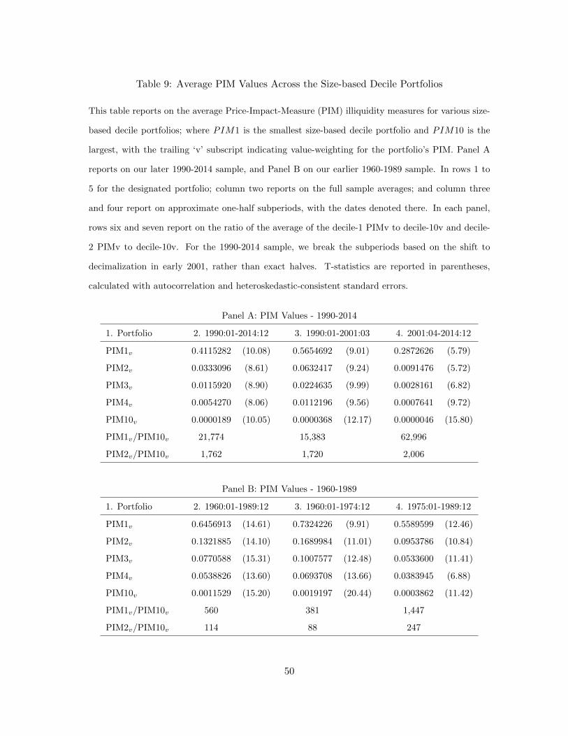
Table 9: Average PIM Values Across the Size-based Decile Portfolios

This table reports on the average Price-Impact-Measure (PIM) illiquidity measures for various size-

based decile portfolios; where PIM1 is the smallest size-based decile portfolio and PIM10 is the

largest, with the trailing ‘v’ subscript indicating value-weighting for the portfolio’s PIM. Panel A

reports on our later 1990-2014 sample, and Panel B on our earlier 1960-1989 sample. In rows 1 to

5 for the designated portfolio; column two reports on the full sample averages; and column three

and four report on approximate one-half subperiods, with the dates denoted there. In each panel,

rows six and seven report on the ratio of the average of the decile-1 PIMv to decile-10v and decile-

2 PIMv to decile-10v. For the 1990-2014 sample, we break the subperiods based on the shift to

decimalization in early 2001, rather than exact halves. T-statistics are reported in parentheses,

calculated with autocorrelation and heteroskedastic-consistent standard errors.

Panel A: PIM Values - 1990-2014

1. Portfolio 2. 1990:01-2014:12 3. 1990:01-2001:03 4. 2001:04-2014:12

PIM1v 0.4115282 (10.08) 0.5654692 (9.01) 0.2872626 (5.79)

PIM2v 0.0333096 (8.61) 0.0632417 (9.24) 0.0091476 (5.72)

PIM3v 0.0115920 (8.90) 0.0224635 (9.99) 0.0028161 (6.82)

PIM4v 0.0054270 (8.06) 0.0112196 (9.56) 0.0007641 (9.72)

PIM10v 0.0000189 (10.05) 0.0000368 (12.17) 0.0000046 (15.80)

PIM1v/PIM10v 21,774 15,383 62,996

PIM2v/PIM10v 1,762 1,720 2,006

Panel B: PIM Values - 1960-1989

1. Portfolio 2. 1960:01-1989:12 3. 1960:01-1974:12 4. 1975:01-1989:12

PIM1v 0.6456913 (14.61) 0.7324226 (9.91) 0.5589599 (12.46)

PIM2v 0.1321885 (14.10) 0.1689984 (11.01) 0.0953786 (10.84)

PIM3v 0.0770588 (15.31) 0.1007577 (12.48) 0.0533600 (11.41)

PIM4v 0.0538826 (13.60) 0.0693708 (13.66) 0.0383945 (6.88)

PIM10v 0.0011529 (15.20) 0.0019197 (20.44) 0.0003862 (11.42)

PIM1v/PIM10v 560 381 1,447

PIM2v/PIM10v 114 88 247

50

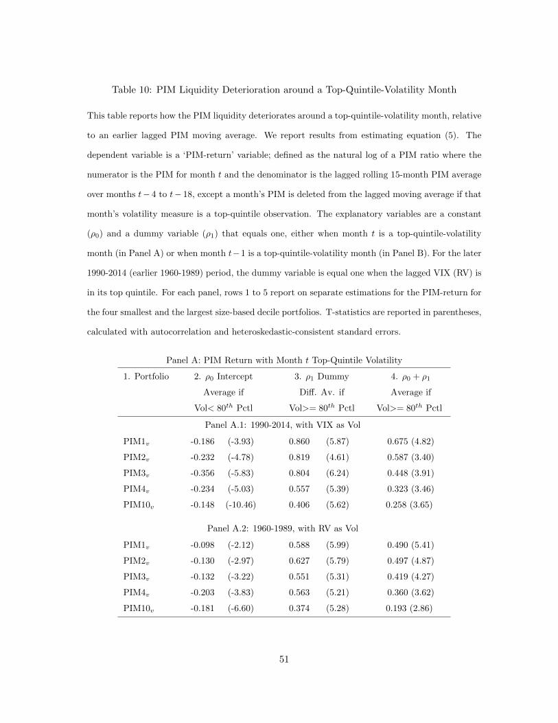
Table 10: PIM Liquidity Deterioration around a Top-Quintile-Volatility Month

This table reports how the PIM liquidity deteriorates around a top-quintile-volatility month, relative

to an earlier lagged PIM moving average. We report results from estimating equation (5). The

dependent variable is a ‘PIM-return’ variable; defined as the natural log of a PIM ratio where the

numerator is the PIM for month t and the denominator is the lagged rolling 15-month PIM average

over months t− 4 to t− 18, except a month’s PIM is deleted from the lagged moving average if that

month’s volatility measure is a top-quintile observation. The explanatory variables are a constant

(ρ0) and a dummy variable (ρ1) that equals one, either when month t is a top-quintile-volatility

month (in Panel A) or when month t−1 is a top-quintile-volatility month (in Panel B). For the later

1990-2014 (earlier 1960-1989) period, the dummy variable is equal one when the lagged VIX (RV) is

in its top quintile. For each panel, rows 1 to 5 report on separate estimations for the PIM-return for

the four smallest and the largest size-based decile portfolios. T-statistics are reported in parentheses,

calculated with autocorrelation and heteroskedastic-consistent standard errors.

Panel A: PIM Return with Month t Top-Quintile Volatility

1. Portfolio 2. ρ0 Intercept 3. ρ1 Dummy 4. ρ0 + ρ1

Average if Diff. Av. if Average if

Vol< 80th Pctl Vol>= 80th Pctl Vol>= 80th Pctl

Panel A.1: 1990-2014, with VIX as Vol

PIM1v -0.186 (-3.93) 0.860 (5.87) 0.675 (4.82)

PIM2v -0.232 (-4.78) 0.819 (4.61) 0.587 (3.40)

PIM3v -0.356 (-5.83) 0.804 (6.24) 0.448 (3.91)

PIM4v -0.234 (-5.03) 0.557 (5.39) 0.323 (3.46)

PIM10v -0.148 (-10.46) 0.406 (5.62) 0.258 (3.65)

Panel A.2: 1960-1989, with RV as Vol

PIM1v -0.098 (-2.12) 0.588 (5.99) 0.490 (5.41)

PIM2v -0.130 (-2.97) 0.627 (5.79) 0.497 (4.87)

PIM3v -0.132 (-3.22) 0.551 (5.31) 0.419 (4.27)

PIM4v -0.203 (-3.83) 0.563 (5.21) 0.360 (3.62)

PIM10v -0.181 (-6.60) 0.374 (5.28) 0.193 (2.86)

51

Table 10: (continued)

Panel B: PIM Return with Month t− 1 Top-Quintile Volatility

1. Portfolio 2. ρ0 Intercept 3. ρ1 Dummy 4. ρ0 + ρ1

Average if Diff. Av. if Average if

Vol< 80th Pctl Vol>= 80th Pctl Vol>= 80th Pctl

Panel B.1: 1990-2014, with VIX as Vol

PIM1v -0.185 (-3.80) 0.855 (5.98) 0.670 (4.95)

PIM2v -0.215 (-4.13) 0.735 (4.36) 0.520 (3.19)

PIM3v -0.348 (-5.64) 0.764 (5.75) 0.416 (3.53)

PIM4v -0.228 (-4.83) 0.525 (5.18) 0.298 (3.25)

PIM10v -0.132 (-7.19) 0.327 (5.07) 0.195 (3.14)

Panel B.2: 1960-1989, with RV as Vol

PIM1v -0.088 (-1.92) 0.540 (5.19) 0.452 (4.65)

PIM2v -0.109 (-2.44) 0.521 (4.59) 0.412 (3.83)

PIM3v -0.115 (-2.80) 0.465 (4.24) 0.351 (3.32)

PIM4v -0.187 (-3.42) 0.484 (4.58) 0.297 (3.10)

PIM10v -0.160 (-5.75) 0.271 (3.64) 0.111 (1.55)

52

Table 11: Differences in SMB Return Distributions following a Top-Quintile Volatility

This table reports on the conditional distribution of monthly returns for SMB and SMB-type

portfolios; conditional on a lagged top-quintile-volatility condition. For each panel, Row 1 reports

on the Fama-French Small-minus-Big (SMB) portfolio and rows 2 to 5 report on the returns of four

other SMB-type portfolio positions, as defined in Table 1. Columns 2 through 10 report on the

return standard deviation, 1st percentile, 5th percentile, 10th percentile, 25th percentile, median,

75th percentile, 90th percentile, 95th percentile, and 99th percentile, in monthly percentage return

units, for the sample or subsample denoted in the panel’s heading. Panel A reports on all monthly

returns. Panel B reports on a ‘Hi-Vol’ subset of returns for months t when there was a lagged

top-quintile VIX/RV condition for any of months t − 1 to t − 6. Panel C reports on a ‘Low-Vol’

subset of returns for months t when there was not a top-quintile VIX/RV condition for month t or

any of the preceding six months t− 1 back to t− 6. The stock-volatility measures are the VIX for

1990-2014 and the rolling RV for 1960-1989.

Panel A: All Monthly Returns

Std. Pctl Pctl Pctl Pctl Pctl Pctl Pctl Pctl Pctl

Dev. 1st 5th 10th 25th 50th 75th 90th 95th 99th

Panel A.1: 1990-2014, n=300 observations

SMB 3.32 -6.54 -4.17 -3.60 -1.68 0.06 1.97 3.67 4.93 7.96

R1v-RL 4.87 -9.33 -6.48 -5.04 -2.45 0.12 2.67 5.29 7.30 15.30

R2v-RL 4.69 -9.08 -6.21 -5.10 -2.40 -0.21 3.20 5.24 7.28 12.45

R3v-RL 4.03 -8.51 -6.19 -4.71 -2.21 0.29 2.79 4.69 6.58 10.45

R4v-RL 3.72 -7.74 -5.53 -4.28 -2.14 0.24 2.32 4.58 5.51 8.75

Panel A.2: 1960-1989, n=360 observations

SMB 2.82 -6.61 -4.07 -3.22 -1.30 0.09 2.00 3.50 4.69 8.09

R1v-RL 4.63 -10.00 -6.40 -4.87 -2.63 0.02 2.83 6.21 8.38 13.91

R2v-RL 3.91 -8.69 -5.60 -4.31 -2.03 -0.06 2.58 5.04 6.74 10.56

R3v-RL 3.61 -8.19 -4.87 -3.90 -1.63 0.06 2.46 4.95 6.05 10.58

R4v-RL 3.39 -8.14 -4.99 -3.52 -1.69 0.03 2.46 4.35 6.08 9.48

53

Table 11: (continued)

Panel B: Monthly SMB Returns following ‘Hi-Vol’ Conditions

Std. Pctl Pctl Pctl Pctl Pctl Pctl Pctl Pctl Pctl

Dev. 1st 5th 10th 25th 50th 75th 90th 95th 99th

Panel B.1: 1990-2014, n=127 observations

SMB 4.21 -7.61 -5.17 -3.70 -1.80 0.48 2.89 4.85 6.25 12.22

R1v-RL 6.16 -13.38 -7.57 -5.65 -2.91 0.42 3.85 7.03 9.49 15.66

R2v-RL 5.82 -10.03 -6.74 -5.50 -2.78 0.13 3.73 7.18 9.07 17.50

R3v-RL 4.82 -8.94 -6.85 -4.99 -1.89 0.31 3.92 6.16 7.34 10.51

R4v-RL 4.51 -9.54 -6.12 -5.00 -2.20 0.58 3.20 5.33 6.78 8.64

Panel B.2: 1960-1989, n=143 observations

SMB 3.24 -7.26 -4.21 -3.43 -1.20 0.52 2.43 4.12 6.16 9.35

R1v-RL 5.17 -10.27 -7.98 -5.18 -2.29 0.68 3.23 6.88 8.83 15.17

R2v-RL 4.50 -8.81 -5.62 -4.48 -2.03 0.46 3.35 6.01 9.02 12.14

R3v-RL 4.10 -8.20 -5.60 -3.79 -1.44 0.71 3.17 5.20 7.93 11.90

R4v-RL 3.91 -8.23 -4.84 -3.82 -1.65 0.78 3.17 5.39 7.00 10.38

Panel C: Monthly SMB Returns following ‘Low-Vol’ Conditions

Std. Pctl Pctl Pctl Pctl Pctl Pctl Pctl Pctl Pctl

Dev. 1st 5th 10th 25th 50th 75th 90th 95th 99th

Panel C.1: 1990-2014, n=164 observations

SMB 2.41 -5.02 -3.92 -3.12 -1.56 -0.13 1.62 2.88 3.48 6.06

R1v-RL 3.67 -8.47 -5.42 -3.92 -2.27 -0.14 2.05 4.36 5.20 8.92

R2v-RL 3.58 -7.05 -5.37 -4.66 -2.29 -0.42 2.34 4.00 5.06 9.11

R3v-RL 3.32 -7.51 -5.08 -4.19 -2.21 0.25 2.51 3.92 4.71 8.49

R4v-RL 3.01 -6.94 -4.86 -3.66 -2.02 0.09 1.87 3.71 4.45 7.36

Panel C.2: 1960-1989, n=207 observations

SMB 2.44 -5.35 -3.93 -2.91 -1.27 -0.10 1.40 3.28 3.93 5.98

R1v-RL 4.22 -9.12 -5.68 -4.63 -2.64 -0.38 2.32 5.76 7.89 11.79

R2v-RL 3.42 -8.42 -5.37 -3.93 -1.94 -0.16 1.98 4.61 5.44 9.33

R3v-RL 3.18 -6.98 -4.77 -4.10 -1.64 -0.17 2.01 4.84 5.46 7.18

R4v-RL 2.93 -6.80 -4.82 -3.12 -1.53 -0.13 1.91 4.24 4.73 6.93

54

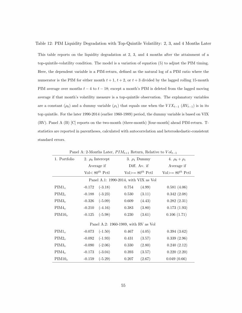
Table 12: PIM Liquidity Degradation with Top-Quintile Volatility: 2, 3, and 4 Months Later

This table reports on the liquidity degradation at 2, 3, and 4 months after the attainment of a

top-quintile-volatility condition. The model is a variation of equation (5) to adjust the PIM timing.

Here, the dependent variable is a PIM-return, defined as the natural log of a PIM ratio where the

numerator is the PIM for either month t+ 1, t+ 2, or t+ 3 divided by the lagged rolling 15-month

PIM average over months t− 4 to t− 18; except a month’s PIM is deleted from the lagged moving

average if that month’s volatility measure is a top-quintile observation. The explanatory variables

are a constant (ρ0) and a dummy variable (ρ1) that equals one when the V IXt−1 (RVt−1) is in its

top quintile. For the later 1990-2014 (earlier 1960-1989) period, the dummy variable is based on VIX

(RV). Panel A (B) [C] reports on the two-month (three-month) [four-month] ahead PIM-return. T-

statistics are reported in parentheses, calculated with autocorrelation and heteroskedastic-consistent

standard errors.

Panel A: 2-Months Later, PIMt+1 Return, Relative to V olt−1

1. Portfolio 2. ρ0 Intercept 3. ρ1 Dummy 4. ρ0 + ρ1

Average if Diff. Av. if Average if

Vol< 80th Pctl Vol>= 80th Pctl Vol>= 80th Pctl

Panel A.1: 1990-2014, with VIX as Vol

PIM1v -0.172 (-3.18) 0.754 (4.99) 0.581 (4.06)

PIM2v -0.188 (-3.23) 0.530 (3.11) 0.342 (2.08)

PIM3v -0.326 (-5.09) 0.609 (4.43) 0.282 (2.31)

PIM4v -0.210 (-4.16) 0.383 (3.80) 0.173 (1.93)

PIM10v -0.125 (-5.98) 0.230 (3.61) 0.106 (1.71)

Panel A.2: 1960-1989, with RV as Vol

PIM1v -0.073 (-1.50) 0.467 (4.05) 0.394 (3.62)

PIM2v -0.092 (-1.93) 0.431 (3.57) 0.339 (2.96)

PIM3v -0.090 (-2.06) 0.330 (2.80) 0.240 (2.12)

PIM4v -0.173 (-3.04) 0.393 (3.57) 0.220 (2.20)

PIM10v -0.159 (-5.29) 0.207 (2.67) 0.049 (0.66)

55

Table 12: (continued)

Panel B: 3-Months Later, PIMt+2 Return, Relative to V olt−1

1. Portfolio 2. ρ0 Intercept 3. ρ1 Dummy 4. ρ0 + ρ1

Average if Diff. Av. if Average if

Vol< 80th Pctl Vol>= 80th Pctl Vol>= 80th Pctl

Panel B.1: 1990-2014, with VIX as Vol

PIM1v -0.160 (-2.72) 0.659 (4.08) 0.499 (3.25)

PIM2v -0.173 (-2.69) 0.393 (2.24) 0.220 (1.33)

PIM3v -0.310 (-4.67) 0.485 (3.46) 0.175 (1.41)

PIM4v -0.205 (-3.81) 0.302 (3.03) 0.098 (1.12)

PIM10v -0.123 (-5.24) 0.166 (2.71) 0.043 (0.73)

Panel B.2: 1960-1989, with RV as Vol

PIM1v -0.061 (-1.18) 0.410 (3.32) 0.349 (3.00)

PIM2v -0.082 (-1.63) 0.372 (2.94) 0.290 (2.42)

PIM3v -0.077 (-1.67) 0.255 (2.10) 0.178 (1.53)

PIM4v -0.167 (-2.86) 0.343 (2.97) 0.176 (1.67)

PIM10v -0.161 (-5.04) 0.164 (2.11) 0.003 (0.04)

Panel C: 4-Months Later, PIMt+3 Return, Relative to V olt−1

1. Portfolio 2. ρ0 Intercept 3. ρ1 Dummy 4. ρ0 + ρ1

Average if Diff. Av. if Average if

Vol< 80th Pctl Vol>= 80th Pctl Vol>= 80th Pctl

Panel C.1: 1990-2014, with VIX as Vol

PIM1v -0.149 (-2.35) 0.568 (3.35) 0.419 (2.60)

PIM2v -0.177 (-2.61) 0.348 (1.99) 0.171 (1.04)

PIM3v -0.307 (-4.56) 0.432 (3.10) 0.125 (1.01)

PIM4v -0.197 (-3.53) 0.211 (2.11) 0.014 (0.16)

PIM10v -0.123 (-4.85) 0.109 (1.88) -0.014 ( -0.26)

Panel C.2: 1960-1989, with RV as Vol

PIM1v -0.051 (-0.92) 0.361 (2.85) 0.310 (2.60)

PIM2v -0.071 (-1.35) 0.310 (2.32) 0.239 (1.88)

PIM3v -0.077 (-1.65) 0.244 (1.90) 0.167 (1.34)

PIM4v -0.167 (-2.83) 0.322 (2.63) 0.155 (1.37)

PIM10v -0.172 (-5.23) 0.160 (2.03) -0.012 (-0.16)

56

Table 13: The Default Yield Spread (DYS) and the Subsequent SMB Premium

This table reports on the relation between the DYS and the subsequent SMB premium. The DYS

is defined as the difference between Moody’s BAA bond yield and the 10-year Treasury Constant

Maturity yield. We repeat the empirical exercise in Table 4, except the conditional dummy variable

is now based on a top-quintile DYS. Comparable to Table 4, we use use a lagged reference 180-

month DYS distribution for determining the top-quintile DYS threshold in a real-time approach. T-

statistics are in parentheses, calculated with autocorrelation and heteroskedastic-consistent standard

errors. The sample period is 1965-2014.

1. Portfolio 2. ψ0 Intercept 3. ψ1 Dummy 4. ψ0 + ψ1 R-Squ.

Average if Diff. Av. if Average if

DYS>= 80th Pctl DYS< 80th Pctl DYS< 80th Pctl

Panel A.1: 3-months Returns

SMB 1.95 (3.01) -1.71 (-2.31) 0.24 (0.60) 1.9%

R2v-RL 2.86 (3.03) -2.89 (-2.69) -0.02 (-0.04) 2.7%

R3v-RL 2.42 (3.15) -1.98 (-2.20) 0.45 (0.87) 1.7%

Panel A.2: 6-months Returns

SMB 3.38 (2.87) -2.64 (-1.98) 0.74 (0.90) 2.2%

R2v-RL 4.69 (2.68) -4.22 (-2.15) 0.46 (0.40) 2.8%

R3v-RL 4.22 (2.92) -3.07 (-1.81) 1.15 (1.10) 2.0%

Panel A.3 12-months Returns

SMB 5.92 (2.30) -3.93 (-1.38) 1.99 (1.09) 2.0%

R2v-RL 8.38 (2.19) -6.89 (-1.67) 1.50 (0.59) 2.9%

R3v-RL 7.23 (2.40) -4.42 (-1.27) 2.80 (1.19) 1.7%

57

Table 14: Size & Beta Double-sorted Portfolio Returns and our Top-Quintile-Volatility State

This table reports on the conditional average returns of size and market-beta double-sorted portfolios,

contingent on our top-quintile-volatility state. We report on the same empirical exercise as in Table 3

and equation (3); except we evaluate the 25 double-sorted value-weighted portfolios from the French

data library, sorted on size and market-beta using the NYSE quintile breakpoints. For each panel,

rows 1 to 6 report on average returns for the designated portfolio position, for subsequent returns at

the 3-, 6-, and 12-month horizon. Panel A (B) reports on beta-based portfolios for stocks within the

smallest (largest) size quintile. Panel C reports on SMB positions between the smallest and largest

size quintile, but separately for high-beta stocks and low-beta stocks. Panel D reports on ‘high-beta

minus low beta’ positions, but separately for stocks in the smallest and largest size quintile. See

Table 3 for the column descriptions and other tabular descriptions.

1. Portfolio 2. ψ0 Intercept 3. ψ1 Dummy 4. ψ0 + ψ1 R-Squ.

Average if Diff. Av. if Average if

Vol>= 80th Pctl Vol< 80th Pctl Vol< 80th Pctl

Panel A.1: Small-Cap Quintile of Stocks, 1990-2014, with VIX as Vol

1. High Beta, 3m 12.78 (4.54) -10.84 (-3.73) 1.94 (1.29) 7.0%

2. High Beta, 6m 25.59 (4.76) -21.62 (-4.18) 3.96 (1.50) 12.9%

3. High Beta, 12m 47.55 (3.80) -37.51 (-3.22) 10.04 (2.54) 17.9%

4. Low Beta, 3m 4.78 (3.07) -2.27 (-1.41) 2.51 (3.14) 1.2%

5. Low Beta, 6m 10.43 (5.49) -5.44 (-2.71) 4.99 (3.12) 3.4%

6. Low Beta, 12m 17.94 (3.81) -5.94 (-1.31) 11.99 (3.89) 1.9%

Panel A.2: Small-Cap Quintile of Stocks, 1960-1989, with RV as Vol

1. High Beta, 3m 10.53 (3.32) -8.58 (-2.59) 1.95 (1.41) 4.9%

2. High Beta, 6m 16.47 (2.71) -10.88 (-1.81) 5.59 (2.06) 3.5%

3. High Beta, 12m 25.57 (2.89) -11.74 (-1.43) 13.83 (2.28) 1.9%

4. Low Beta, 3m 7.12 (4.42) -3.84 (-2.25) 3.28 (3.96) 3.1%

5. Low Beta, 6m 12.78 (3.85) -5.42 (-1.64) 7.37 (4.44) 2.6%

6. Low Beta, 12m 22.96 (4.42) -6.49 (-1.35) 16.47 (4.30) 1.6%

Panel B.1: Large-Cap Quintile of Stocks, 1990-2014, with VIX as Vol

1. High Beta, 3m 10.24 (3.57) -8.51 (-2.90) 1.73 (1.44) 6.6%

2. High Beta, 6m 17.06 (2.86) -12.54 (-2.20) 4.53 (2.03) 6.3%

3. High Beta, 12m 24.60 (2.52) -12.02 (-1.39) 12.58 (2.63) 2.7%

4. Low Beta, 3m 2.41 (1.98) -0.05 (-0.04) 2.36 (4.24) 0.0%

5. Low Beta, 6m 4.85 (2.72) -0.13 (-0.08) 4.72 (4.22) 0.0%

6. Low Beta, 12m 7.52 (2.40) 2.87 (1.00) 10.40 (4.17) 0.8%

Panel B.2: Large-Cap Quintile of Stocks, 1960-1989, with RV as Vol

1. High Beta, 3m 5.83 (2.53) -5.17 (-2.07) 0.65 (0.54) 2.7%

2. High Beta, 6m 8.57 (1.92) -6.35 (-1.35) 2.21 (0.96) 1.9%

3. High Beta, 12m 11.99 (2.43) -7.26 (-1.30) 4.74 (1.09) 1.4%

4. Low Beta, 3m 4.03 (3.61) -1.26 (-1.06) 2.77 (4.40) 0.6%

5. Low Beta, 6m 6.59 (2.56) -0.45 (-0.17) 6.14 (4.70) 0.0%

6. Low Beta, 12m 13.95 (3.91) -1.63 (-0.44) 12.32 (4.09) 0.2%

58

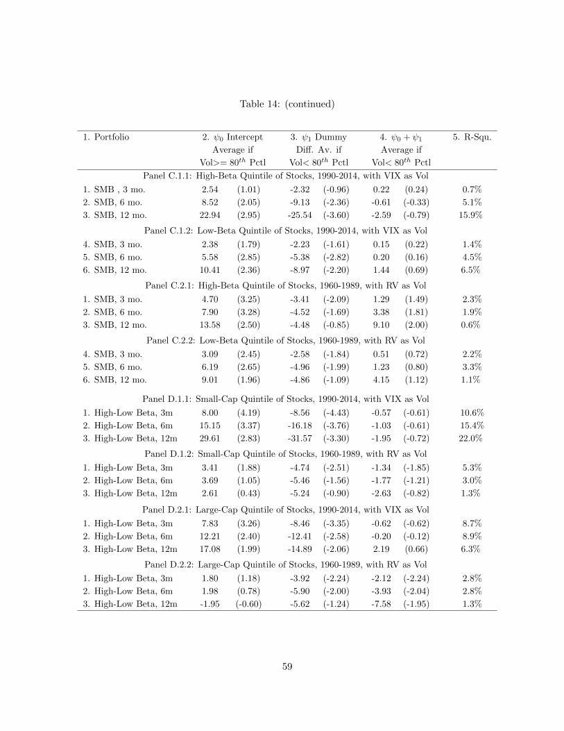
Table 14: (continued)

1. Portfolio 2. ψ0 Intercept 3. ψ1 Dummy 4. ψ0 + ψ1 5. R-Squ.

Average if Diff. Av. if Average if

Vol>= 80th Pctl Vol< 80th Pctl Vol< 80th Pctl

Panel C.1.1: High-Beta Quintile of Stocks, 1990-2014, with VIX as Vol

1. SMB , 3 mo. 2.54 (1.01) -2.32 (-0.96) 0.22 (0.24) 0.7%

2. SMB, 6 mo. 8.52 (2.05) -9.13 (-2.36) -0.61 (-0.33) 5.1%

3. SMB, 12 mo. 22.94 (2.95) -25.54 (-3.60) -2.59 (-0.79) 15.9%

Panel C.1.2: Low-Beta Quintile of Stocks, 1990-2014, with VIX as Vol

4. SMB, 3 mo. 2.38 (1.79) -2.23 (-1.61) 0.15 (0.22) 1.4%

5. SMB, 6 mo. 5.58 (2.85) -5.38 (-2.82) 0.20 (0.16) 4.5%

6. SMB, 12 mo. 10.41 (2.36) -8.97 (-2.20) 1.44 (0.69) 6.5%

Panel C.2.1: High-Beta Quintile of Stocks, 1960-1989, with RV as Vol

1. SMB, 3 mo. 4.70 (3.25) -3.41 (-2.09) 1.29 (1.49) 2.3%

2. SMB, 6 mo. 7.90 (3.28) -4.52 (-1.69) 3.38 (1.81) 1.9%

3. SMB, 12 mo. 13.58 (2.50) -4.48 (-0.85) 9.10 (2.00) 0.6%

Panel C.2.2: Low-Beta Quintile of Stocks, 1960-1989, with RV as Vol

4. SMB, 3 mo. 3.09 (2.45) -2.58 (-1.84) 0.51 (0.72) 2.2%

5. SMB, 6 mo. 6.19 (2.65) -4.96 (-1.99) 1.23 (0.80) 3.3%

6. SMB, 12 mo. 9.01 (1.96) -4.86 (-1.09) 4.15 (1.12) 1.1%

Panel D.1.1: Small-Cap Quintile of Stocks, 1990-2014, with VIX as Vol

1. High-Low Beta, 3m 8.00 (4.19) -8.56 (-4.43) -0.57 (-0.61) 10.6%

2. High-Low Beta, 6m 15.15 (3.37) -16.18 (-3.76) -1.03 (-0.61) 15.4%

3. High-Low Beta, 12m 29.61 (2.83) -31.57 (-3.30) -1.95 (-0.72) 22.0%

Panel D.1.2: Small-Cap Quintile of Stocks, 1960-1989, with RV as Vol

1. High-Low Beta, 3m 3.41 (1.88) -4.74 (-2.51) -1.34 (-1.85) 5.3%

2. High-Low Beta, 6m 3.69 (1.05) -5.46 (-1.56) -1.77 (-1.21) 3.0%

3. High-Low Beta, 12m 2.61 (0.43) -5.24 (-0.90) -2.63 (-0.82) 1.3%

Panel D.2.1: Large-Cap Quintile of Stocks, 1990-2014, with VIX as Vol

1. High-Low Beta, 3m 7.83 (3.26) -8.46 (-3.35) -0.62 (-0.62) 8.7%

2. High-Low Beta, 6m 12.21 (2.40) -12.41 (-2.58) -0.20 (-0.12) 8.9%

3. High-Low Beta, 12m 17.08 (1.99) -14.89 (-2.06) 2.19 (0.66) 6.3%

Panel D.2.2: Large-Cap Quintile of Stocks, 1960-1989, with RV as Vol

1. High-Low Beta, 3m 1.80 (1.18) -3.92 (-2.24) -2.12 (-2.24) 2.8%

2. High-Low Beta, 6m 1.98 (0.78) -5.90 (-2.00) -3.93 (-2.04) 2.8%

3. High-Low Beta, 12m -1.95 (-0.60) -5.62 (-1.24) -7.58 (-1.95) 1.3%

59

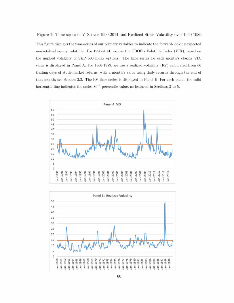
Figure 1: Time series of VIX over 1990-2014 and Realized Stock Volatility over 1960-1989

This figure displays the time-series of our primary variables to indicate the forward-looking expected

market-level equity volatility. For 1990-2014, we use the CBOE’s Volatility Index (VIX), based on

the implied volatility of S&P 500 index options. The time series for each month’s closing VIX

value is displayed in Panel A. For 1960-1989, we use a realized volatility (RV) calculated from 66

trading days of stock-market returns, with a month’s value using daily returns through the end of

that month; see Section 2.3. The RV time series is displayed in Panel B. For each panel, the solid

horizontal line indicates the series 80th percentile value, as featured in Sections 3 to 5.

0

5

10

15

20

25

30

35

40

45

50

55

60

Jan

-19

90

Jan

-19

91

Jan

-19

92

Jan

-19

93

Jan

-19

94

Jan

-19

95

Jan

-19

96

Jan

-19

97

Jan

-19

98

Jan

-19

99

Jan

-20

00

Jan

-20

01

Jan

-20

02

Jan

-20

03

Jan

-20

04

Jan

-20

05

Jan

-20

06

Jan

-20

07

Jan

-20

08

Jan

-20

09

Jan

-20

10

Jan

-20

11

Jan

-20

12

Jan

-20

13

Jan

-20

14

Panel A: VIX

0

5

10

15

20

25

30

35

40

45

50

Jan

-19

60

Jan

-19

61

Jan

-19

62

Jan

-19

63

Jan

-19

64

Jan

-19

65

Jan

-19

66

Jan

-19

67

Jan

-19

68

Jan

-19

69

Jan

-19

70

Jan

-19

71

Jan

-19

72

Jan

-19

73

Jan

-19

74

Jan

-19

75

Jan

-19

76

Jan

-19

77

Jan

-19

78

Jan

-19

79

Jan

-19

80

Jan

-19

81

Jan

-19

82

Jan

-19

83

Jan

-19

84

Jan

-19

85

Jan

-19

86

Jan

-19

87

Jan

-19

88

Jan

-19

89

Panel B: Realized Volatility

60

Figure 2: Time Series of our ‘PIM-Return’ Variables

This figure displays selected time-series of our primary ‘PIM-return’ variables, as defined in equation

(5) and used in Table 10. For a given decile portfolio, the PIM-return equals the log of a PIM ratio,

where the PIM from month t is the numerator and the average PIM over months t−4 to t−18 is the

denominator; but with the lagged PIM moving average excluding months that are a top-quintile-

volatility observation month. Thus, the PIM-return is in the spirit of a continuously-compounded

percentage return. Panels A and B report this PIM-return for the second smallest and largest size

decile over the 1990-2014 segment of our sample; months with a marker on the value 4 on the vertical

axis indicate a top-quintile-VIX observation. Panels C and D report this PIM-return for the second

smallest and largest size decile over the 1960-1989 segment of our sample; months with a marker on

the value 2 on the vertical axis indicate a top-quintile-RV observation.

-2

-1

0

1

2

3

4

Jun

-19

91

Jun

-19

92

Jun

-19

93

Jun

-19

94

Jun

-19

95

Jun

-19

96

Jun

-19

97

Jun

-19

98

Jun

-19

99

Jun

-20

00

Jun

-20

01

Jun

-20

02

Jun

-20

03

Jun

-20

04

Jun

-20

05

Jun

-20

06

Jun

-20

07

Jun

-20

08

Jun

-20

09

Jun

-20

10

Jun

-20

11

Jun

-20

12

Jun

-20

13

Jun

-20

14

Panel A: PIM Return for Second Smallest Size Decile, 1990-2014

-2

-1

0

1

2

3

4

Jun

-19

91

Jun

-19

92

Jun

-19

93

Jun

-19

94

Jun

-19

95

Jun

-19

96

Jun

-19

97

Jun

-19

98

Jun

-19

99

Jun

-20

00

Jun

-20

01

Jun

-20

02

Jun

-20

03

Jun

-20

04

Jun

-20

05

Jun

-20

06

Jun

-20

07

Jun

-20

08

Jun

-20

09

Jun

-20

10

Jun

-20

11

Jun

-20

12

Jun

-20

13

Jun

-20

14

Panel B: PIM Return for Largest Size Decile, 1990-2014

61

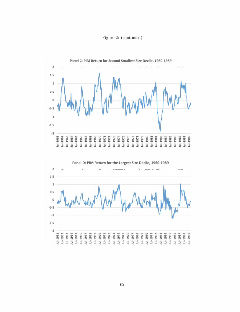
Figure 2: (continued)

-2

-1.5

-1

-0.5

0

0.5

1

1.5

2

Jul-

19

61

Jul-

19

62

Jul-

19

63

Jul-

19

64

Jul-

19

65

Jul-

19

66

Jul-

19

67

Jul-

19

68

Jul-

19

69

Jul-

19

70

Jul-

19

71

Jul-

19

72

Jul-

19

73

Jul-

19

74

Jul-

19

75

Jul-

19

76

Jul-

19

77

Jul-

19

78

Jul-

19

79

Jul-

19

80

Jul-

19

81

Jul-

19

82

Jul-

19

83

Jul-

19

84

Jul-

19

85

Jul-

19

86

Jul-

19

87

Jul-

19

88

Jul-

19

89

Panel C: PIM Return for Second Smallest Size Decile, 1960-1989

-2

-1.5

-1

-0.5

0

0.5

1

1.5

2

Jul-

19

61

Jul-

19

62

Jul-

19

63

Jul-

19

64

Jul-

19

65

Jul-

19

66

Jul-

19

67

Jul-

19

68

Jul-

19

69

Jul-

19

70

Jul-

19

71

Jul-

19

72

Jul-

19

73

Jul-

19

74

Jul-

19

75

Jul-

19

76

Jul-

19

77

Jul-

19

78

Jul-

19

79

Jul-

19

80

Jul-

19

81

Jul-

19

82

Jul-

19

83

Jul-

19

84

Jul-

19

85

Jul-

19

86

Jul-

19

87

Jul-

19

88

Jul-

19

89

Panel D: PIM Return for the Largest Size Decile, 1960-1989

62

Appendix A1: VIX/RV and the Subsequent Stock-Market Volatility

This table reports on the relation between VIX/RV and the subsequent stock-market volatility.

Relative to the closing VIX/RV on day t− 1, we investigate the subsequent realized volatility (RV)

of stock market returns as the dependent variables, for both the subsequent 22-trading-day (days t

to t+ 21) and 66-trading-day (days t to t+ 65) periods. For the realized stock market volatility, we

annualize the sample standard deviation of the 22 or 66 daily returns. Panel A reports on the 1990-

2014 period with the lagged VIX as the explanatory term. Panel B reports on the 1960-1989 period,

with our lagged rolling 66-trading-day RV as the explanatory term. We report on two specifications:

(1) estimating a simple continuous linear regression with the lagged VIX/RV as the explanatory

variable and the subsequent RV as the dependent variable (shown in columns 1 to 3, in Panels A.1

and B.1); and (2) estimating the same model, but with the log transformation of the VIX and RV

variables to reduce positive skewness (shown in column 4 to 6, in Panels A.2 and B.2). T-statistics

are reported in parentheses, calculated with autocorrelation and heteroskedastic-consistent standard

errors.

Panel A: RV Linear Regression, the Explanatory Variable is VIX or the Log(VIX): 1990-2014

Panel A.1: Simple (Col. 1-3) Panel A.2: Log (Col. 4 -6)

1. RV 2. λ1 Coeff. 3. R2 4. ln(RV) 5. λ1 Coeff. 6. R2

Dep. Variable on VIX Dep. Variable on log(VIX)

St.Mkt.Vol-22 0.887 (14.04) 60.0% ln(St.Mkt.Vol-22) 1.07 (25.46) 59.9%

St.Mkt.Vol-66 0.723 (12.39) 45.3% ln(St.Mkt.Vol-66) 0.92 (15.63) 52.9%

Panel B: RV Linear Regression, the Explanatory Variable is RV or the Log(RV): 1960-1989

Panel B.1: Simple (Col. 1-3) Panel B.2: Log (Col. 4 -6)

1. RV 2. λ1 Coeff. 3. R2 4. ln(RV) 5. λ1 Coeff. 6. R2

Dep. Variable on RV Dep. Variable on ln(RV)

St.Mkt.Vol-22 0.699 (10.16) 41.9% ln(St.Mkt.Vol-22) 0.762 (21.43) 49.3%

St.Mkt.Vol-66 0.595 (9.84) 35.5% ln(St.Mkt.Vol-66) 0.670 (16.81) 45.0%

63

Appendix A2: Price Impact Measure (PIM) Calculation

The PIM for an individual stock is estimated using the daily return and volume data over the month,

where the value may be interpreted as the absolute return per $1000 of trading volume. Since Amihud’s

PIM measure estimates illiquidity, a lower PIM indicates higher liquidity. While forming portfolio-level

measures of PIM each month, we include only those stocks that meet the following conditions: (a) there

should be at least 15 observations to estimate a stock’s liquidity PIM, (b) it should be an ordinary share

(CRSP share code 10 or 11), (c) it should be listed on NYSE/AMEX/NASDAQ (CRSP exchange code 1

or 2 or 3), (d) the share price should be between $5 and $1000 at the end of previous month, (e) the first

day (or the last day) that the stock appears (or disappears) on CRSP should not fall during the previous

month.

64

Appendix A3: SMB and the Top-Quintile-Volatility Condition: Subperiod Analysis

This appendix table repeats the empirical exercise in Table 3 of the main text, but for inclusive

one-half subperiods for each of our two primary sample segments (1990-2014 and 1960-1989) for

each of the three return horizons.

1. Portfolio 2. ψ0 Intercept 3. ψ1 Dummy 4. ψ0 + ψ1 R-Squ.

Average if Diff. Av. if Average if

Vol>= 80th Pctl Vol< 80th Pctl Vol< 80th Pctl

Panel A.1: 3-Month Returns; 1st Half, 1990:01 - 2002:06, with VIX as Vol

SMB 2.13 (1.18) -2.09 (-1.10) 0.04 (0.05) 1.4%

R2v-RL 3.20 (1.24) -2.80 (-1.05) 0.40 (0.33) 1.3%

Panel A.2: 3-Month Returns; 2nd Half, 2002:07 - 2014:12, with VIX as Vol

SMB 2.96 (4.05) -2.68 (-3.32) 0.28 (0.52) 7.2%

R2v-RL 3.59 (2.36) -3.58 (-2.26) 0.01 (0.01) 5.1%

Panel A.3: 3-Month Returns; 1st Half, 1960:01 - 1974:12, with RV as Vol

SMB 0.73 (0.46) -0.63 (-0.36) 0.10 (0.12) 0.2%

R2v-RL 1.33 (0.71) -1.30 (-0.60) 0.03 (0.60) 0.4%

Panel A.4: 3-Month Returns; 2nd Half, 1975:01 - 1989:12, with RV as Vol

SMB 5.23 (5.43) -4.98 (-4.72) 0.25 (0.43) 16.0%

R2v-RL 6.89 (4.90) -6.85 (-4.53) 0.04 (0.05) 14.9%

Panel B.1: 6-Month Returns; 1st Half, 1990:01 - 2002:06, with VIX as Vol

SMB 4.88 (1.53) -5.42 (-1.89) -0.53 (-0.41) 5.7%

R2v-RL 7.76 (1.93) -8.07 (-2.26) -0.31 (-0.15) 6.0%

Panel B.2: 6-Month Returns; 2nd Half, 2002:07 - 2014:12, with VIX as Vol

SMB 7.15 (3.83) -6.88 (-3.72) 0.27 (0.30) 20.8%

R2v-RL 8.77 (2.94) -9.07 (-3.09) -0.31 (-0.22) 15.0%

Panel B.3: 6-Month Returns; 1st Half, 1960:01 - 1974:12, with RV as Vol

SMB 2.67 (0.80) -2.51 (-0.72) 0.16 (0.10) 1.0%

R2v-RL 5.16 (1.40) -5.22 (-1.34) -0.06 (-0.03) 2.5%

Panel B.4: 6-Month Returns; 2nd Half, 1975:01 - 1989:12, with RV as Vol

SMB 7.18 (4.00) -5.75 (-3.02) 1.43 (1.12) 9.2%

R2v-RL 9.27 (4.08) -7.91 (-3.12) 1.36 (0.73) 8.7%

Panel C.1: 12-Month Returns; 1st Half, 1990:01 - 2002:06, with VIX as Vol

SMB 9.38 (1.77) -10.55 (-2.52) -1.16 (-0.53) 10.3%

R2v-RL 16.18 (2.12) -17.06 (-3.05) -0.88 (-0.23) 11.1%

Panel C.2: 12-Month Returns; 2nd Half, 2002:07 - 2014:12, with VIX as Vol

SMB 13.40 (2.96) -12.50 (-2.81) 0.90 (0.62) 29.5%

R2v-RL 16.61 (2.34) -16.71 (-2.40) -0.10 (-0.04) 23.2%

Panel C.3: 12-Month Returns; 1st Half, 1960:01 - 1974:12, with RV as Vol

SMB 6.56 (0.80) -5.78 (-0.78) 0.78 (0.21) 1.6%

R2v-RL 10.80 (1.08) -9.98 (-1.12) 0.82 (0.16) 2.7%

Panel C.4: 12-Month Returns; Second-Half: 1975:01 - 1989:12

SMB 9.21 (3.61) -4.28 (-1.23) 4.93 (1.42) 1.9%

R2v-RL 11.41 (2.98) -6.02 (-1.24) 5.39 (1.13) 2.0%

65

Appendix A4: SMB Average Returns Following a Top Quintile Stock-Volatility Measure II

This appendix table repeats the empirical exercise in Table 3 of the main text, but where the small-

cap portfolios, R1 to R4 are now equal-weighted portfolios denoted with a trailing subscript

e (rather than value-weighted as in Table 3). Otherwise, the empirical exercise is exactly as

explained in Table 3. RL is the largest size-based decile portfolio, value-weighted, reported below

for comparison to the small-cap portfolios. T-statistics are reported in parentheses, calculated with

autocorrelation and heteroskedastic-consistent standard errors.

1. Portfolio 2. ψ0 Intercept 3. ψ1 Dummy 4. ψ0 + ψ1 R-Squ.

Average if Diff. Av. if Average if

Vol>= 80th Pctl Vol< 80th Pctl Vol< 80th Pctl

Panel A.1: 3-months Returns, 1990-2014, with VIX as Vol

R1e-RL 5.94 (3.01) -5.26 (-2.65) 0.68 (0.73) 4.1%

R2e-RL 4.73 (2.84) -5.20 (-3.08) -0.47 (-0.66) 6.0%

R3e-RL 4.34 (3.07) -4.42 (-3.03) -0.08 (-0.12) 5.7%

R4e-RL 3.93 (2.86) -4.23 (-3.01) -0.30 (-0.52) 6.2%

R1e 10.90 (4.37) -8.25 (-3.24) 2.66 (2.15) 6.2%

R2e 9.69 (4.22) -8.18 (-3.43) 1.51 (1.40) 7.1%

R3e 9.30 (4.42) -7.40 (-3.36) 1.90 (1.87) 6.7%

R4e 8.89 (4.26) -7.21 (-3.33) 1.68 (1.75) 6.8%

RL 4.96 (3.21) -2.98 (-1.92) 1.98 (2.89) 2.6%

Panel A.2: 3-months Returns, 1960-1989, with RV as Vol

R1e-RL 6.56 (3.65) -5.87 (-2.89) 0.69 (0.71) 4.9%

R2e-RL 4.80 (3.40) -4.86 (-3.10) -0.06 (-0.08) 5.8%

R3e-RL 4.81 (3.88) -4.57 (-3.30) 0.24 (0.39) 6.4%

R4e-RL 4.48 (3.65) -4.30 (-3.17) 0.19 (0.31) 6.3%

R1e 10.56 (4.01) -7.59 (-2.73) 2.97 (2.47) 4.7%

R2e 8.80 (3.73) -6.58 (-2.69) 2.23 (2.22) 4.6%

R3e 8.82 (3.98) -6.29 (-2.73) 2.52 (2.65) 4.6%

R4e 8.49 (4.01) -6.02 (-2.73) 2.47 (2.66) 4.5%

RL 4.00 (3.04) -1.72 (-1.27) 2.28 (3.73) 0.9%

66

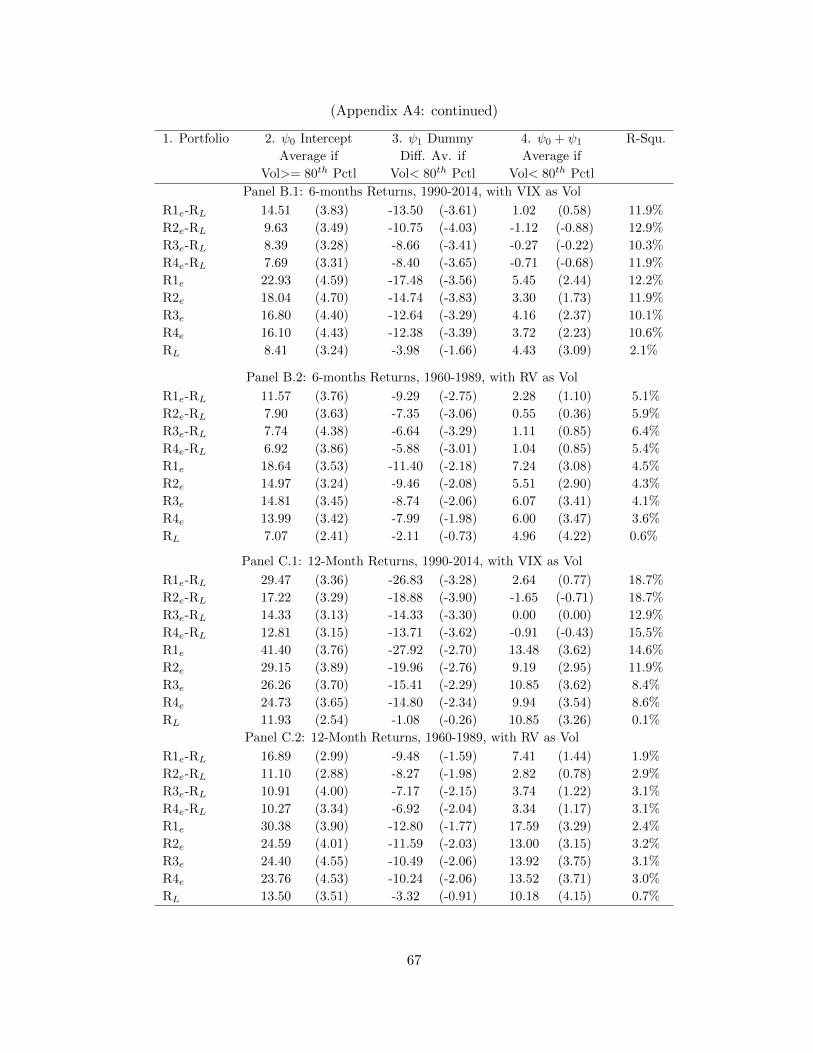
(Appendix A4: continued)

1. Portfolio 2. ψ0 Intercept 3. ψ1 Dummy 4. ψ0 + ψ1 R-Squ.

Average if Diff. Av. if Average if

Vol>= 80th Pctl Vol< 80th Pctl Vol< 80th Pctl

Panel B.1: 6-months Returns, 1990-2014, with VIX as Vol

R1e-RL 14.51 (3.83) -13.50 (-3.61) 1.02 (0.58) 11.9%

R2e-RL 9.63 (3.49) -10.75 (-4.03) -1.12 (-0.88) 12.9%

R3e-RL 8.39 (3.28) -8.66 (-3.41) -0.27 (-0.22) 10.3%

R4e-RL 7.69 (3.31) -8.40 (-3.65) -0.71 (-0.68) 11.9%

R1e 22.93 (4.59) -17.48 (-3.56) 5.45 (2.44) 12.2%

R2e 18.04 (4.70) -14.74 (-3.83) 3.30 (1.73) 11.9%

R3e 16.80 (4.40) -12.64 (-3.29) 4.16 (2.37) 10.1%

R4e 16.10 (4.43) -12.38 (-3.39) 3.72 (2.23) 10.6%

RL 8.41 (3.24) -3.98 (-1.66) 4.43 (3.09) 2.1%

Panel B.2: 6-months Returns, 1960-1989, with RV as Vol

R1e-RL 11.57 (3.76) -9.29 (-2.75) 2.28 (1.10) 5.1%

R2e-RL 7.90 (3.63) -7.35 (-3.06) 0.55 (0.36) 5.9%

R3e-RL 7.74 (4.38) -6.64 (-3.29) 1.11 (0.85) 6.4%

R4e-RL 6.92 (3.86) -5.88 (-3.01) 1.04 (0.85) 5.4%

R1e 18.64 (3.53) -11.40 (-2.18) 7.24 (3.08) 4.5%

R2e 14.97 (3.24) -9.46 (-2.08) 5.51 (2.90) 4.3%

R3e 14.81 (3.45) -8.74 (-2.06) 6.07 (3.41) 4.1%

R4e 13.99 (3.42) -7.99 (-1.98) 6.00 (3.47) 3.6%

RL 7.07 (2.41) -2.11 (-0.73) 4.96 (4.22) 0.6%

Panel C.1: 12-Month Returns, 1990-2014, with VIX as Vol

R1e-RL 29.47 (3.36) -26.83 (-3.28) 2.64 (0.77) 18.7%

R2e-RL 17.22 (3.29) -18.88 (-3.90) -1.65 (-0.71) 18.7%

R3e-RL 14.33 (3.13) -14.33 (-3.30) 0.00 (0.00) 12.9%

R4e-RL 12.81 (3.15) -13.71 (-3.62) -0.91 (-0.43) 15.5%

R1e 41.40 (3.76) -27.92 (-2.70) 13.48 (3.62) 14.6%

R2e 29.15 (3.89) -19.96 (-2.76) 9.19 (2.95) 11.9%

R3e 26.26 (3.70) -15.41 (-2.29) 10.85 (3.62) 8.4%

R4e 24.73 (3.65) -14.80 (-2.34) 9.94 (3.54) 8.6%

RL 11.93 (2.54) -1.08 (-0.26) 10.85 (3.26) 0.1%

Panel C.2: 12-Month Returns, 1960-1989, with RV as Vol

R1e-RL 16.89 (2.99) -9.48 (-1.59) 7.41 (1.44) 1.9%

R2e-RL 11.10 (2.88) -8.27 (-1.98) 2.82 (0.78) 2.9%

R3e-RL 10.91 (4.00) -7.17 (-2.15) 3.74 (1.22) 3.1%

R4e-RL 10.27 (3.34) -6.92 (-2.04) 3.34 (1.17) 3.1%

R1e 30.38 (3.90) -12.80 (-1.77) 17.59 (3.29) 2.4%

R2e 24.59 (4.01) -11.59 (-2.03) 13.00 (3.15) 3.2%

R3e 24.40 (4.55) -10.49 (-2.06) 13.92 (3.75) 3.1%

R4e 23.76 (4.53) -10.24 (-2.06) 13.52 (3.71) 3.0%

RL 13.50 (3.51) -3.32 (-0.91) 10.18 (4.15) 0.7%

67

Appendix A5: SMB Average Returns Following a Top Quintile Volatility: 1-month Returns

This table reports how small-minus-big portfolio returns are different following top quintile

observations of our stock-volatility measures; as in Table 3, except here we examine the shorter

one-month horizon. We report on average 1-month returns over month t+ 1, relative to the closing

volatility measure from month t − 1. For each panel, column two denotes the average return for

periods when the lagged volatility measures (V olt−1) was >= its 80th percentile as the base intercept

case ψ0; column three indicates the difference in average returns following months where the V olt−1

level was< its 80th percentile with the ψ1 coefficient on the conditional dummy variable, as compared

to the average return for the base high-Vol case. Column four indicates the simple average return

following the relatively lower V ol condition (=ψ0 + ψ1). The final column gives the regression’s

R-squared value. Panel A reports results for the 1990-2014 period, conditional on VIX. Panel B

reports results for the 1960-1989 period, conditional on our 66-trading-day rolling RV. T-statistics

are reported in parentheses, calculated with autocorrelation and heteroskedastic-consistent standard

errors.

1. Portfolio 2. ψ0 Intercept 3. ψ1 Dummy 4. ψ0 + ψ1 R-Squ.

Average if Diff. Av. if Average if

Vol>= 80th Pctl Vol< 80th Pctl Vol< 80th Pctl

Panel A: 1990-2014 with a top-quintile VIX Threshold

SMB 0.86 (1.68) -0.85 (-1.50) 0.01 (0.04) 1.1%

R1v-RL 0.67 (0.84) -0.48 (-0.55) 0.19 (0.59) 0.2%

R2v-RL 1.09 (1.42) -1.06 (-1.28) 0.03 (0.09) 0.8%

R3v-RL 0.95 (1.63) -0.86 (-1.33) 0.10 (0.38) 0.7%

R4v-RL 0.73 (1.34) -0.72 (-1.18) 0.02 (0.08) 0.6%

R1v 2.75 (2.85) -2.03 (-1.95) 0.73 (1.75) 1.8%

R2v 3.17 (3.11) -2.61 (-2.41) 0.56 (1.39) 2.7%

R3v 3.04 (3.53) -2.41 (-2.61) 0.63 (1.65) 2.7%

R4v 2.82 (3.38) -2.27 (-2.54) 0.55 (1.53) 2.6%

RL 2.08 (3.18) -1.55 (-2.24) 0.53 (2.12) 2.2%

Panel B: 1960-1989 with a top-quintile RV Threshold

SMB 1.35 (3.67) -1.39 (-3.37) -0.04 (-0.24) 3.9%

R1v-RL 1.83 (3.15) -1.87 (-2.86) -0.03 (-0.11) 2.6%

R2v-RL 1.78 (3.45) -1.87 (-3.26) -0.09 (-0.37) 3.7%

R3v-RL 1.76 (3.64) -1.70 (-3.20) 0.05 (0.24) 3.6%

R4v-RL 1.62 (3.55) -1.59 (-3.14) 0.03 (0.14) 3.5%

R1v 3.64 (4.55) -3.02 (-3.35) 0.62 (1.45) 3.5%

R2v 3.59 (4.56) -3.03 (-3.44) 0.56 (1.43) 3.9%

R3v 3.57 (4.62) -2.86 (-3.32) 0.70 (1.84) 3.6%

R4v 3.43 (4.66) -2.75 (-3.31) 0.68 (1.83) 3.6%

RL 1.81 (3.23) -1.16 (-1.89) 0.65 (2.62) 1.2%

68

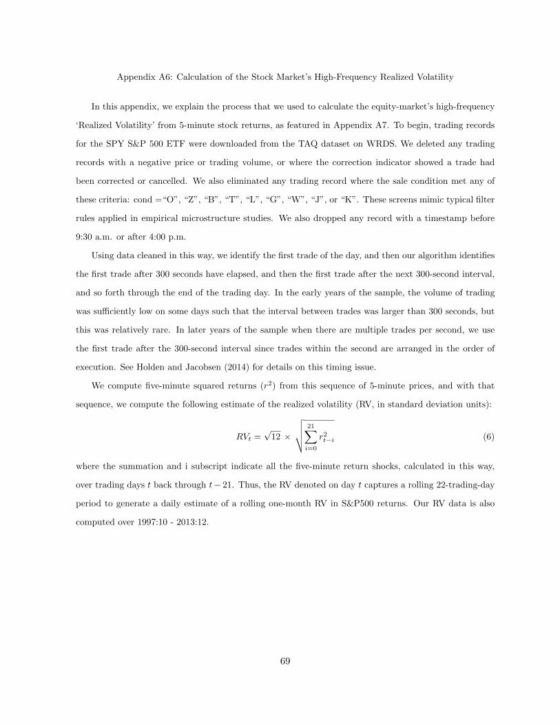
Appendix A6: Calculation of the Stock Market’s High-Frequency Realized Volatility

In this appendix, we explain the process that we used to calculate the equity-market’s high-frequency

‘Realized Volatility’ from 5-minute stock returns, as featured in Appendix A7. To begin, trading records

for the SPY S&P 500 ETF were downloaded from the TAQ dataset on WRDS. We deleted any trading

records with a negative price or trading volume, or where the correction indicator showed a trade had

been corrected or cancelled. We also eliminated any trading record where the sale condition met any of

these criteria: cond =“O”, “Z”, “B”, “T”, “L”, “G”, “W”, “J”, or “K”. These screens mimic typical filter

rules applied in empirical microstructure studies. We also dropped any record with a timestamp before

9:30 a.m. or after 4:00 p.m.

Using data cleaned in this way, we identify the first trade of the day, and then our algorithm identifies

the first trade after 300 seconds have elapsed, and then the first trade after the next 300-second interval,

and so forth through the end of the trading day. In the early years of the sample, the volume of trading

was sufficiently low on some days such that the interval between trades was larger than 300 seconds, but

this was relatively rare. In later years of the sample when there are multiple trades per second, we use

the first trade after the 300-second interval since trades within the second are arranged in the order of

execution. See Holden and Jacobsen (2014) for details on this timing issue.

We compute five-minute squared returns (r2) from this sequence of 5-minute prices, and with that

sequence, we compute the following estimate of the realized volatility (RV, in standard deviation units):

RVt =√

12 ×

√√√√ 21∑i=0

r2t−i (6)

where the summation and i subscript indicate all the five-minute return shocks, calculated in this way,

over trading days t back through t− 21. Thus, the RV denoted on day t captures a rolling 22-trading-day

period to generate a daily estimate of a rolling one-month RV in S&P500 returns. Our RV data is also

computed over 1997:10 - 2013:12.

69

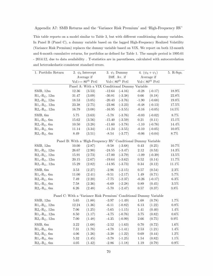
Appendix A7: SMB Returns and the ‘Variance Risk Premium’ and ‘High-Frequency RV’

This table reports on a model similar to Table 3, but with different conditioning dummy variables.

In Panel B (Panel C), a dummy variable based on the lagged High-Frequency Realized Volatility

(Variance Risk Premium) replaces the dummy variable based on VIX. We report on both 12-month

and 6-month cumulative returns, for portfolios as defined for Table 1. The sample period is 1995:01

- 2014:12, due to data availability . T-statistics are in parentheses, calculated with autocorrelation

and heteroskedastic-consistent standard errors.

1. Portfolio Return 2. ψ0 Intercept 3. ψ1 Dummy 4. (ψ0 + ψ1) 5. R-Squ.

Average if Diff. Av. if Average if

Vol>= 80th Pctl Vol< 80th Pctl Vol< 80th Pctl

Panel A: With a VIX Conditional Dummy Variable

SMB, 12m 12.36 (3.53) -12.64 (-4.16) -0.28 (-0.17) 18.9%

R1e-RL, 12m 31.47 (3.09) -30.81 (-3.38) 0.66 (0.18) 22.8%

R2e-RL, 12m 18.53 (3.05) -20.43 (-3.76) -1.90 (-0.68) 19.8%

R1v-RL, 12m 23.38 (2.75) -23.86 (-3.23) -0.48 (-0.13) 17.5%

R2v-RL, 12m 16.79 (3.08) -16.95 (-3.55) -0.16 (-0.05) 14.5%

SMB, 6m 5.75 (3.63) -5.78 (-3.76) -0.03 (-0.02) 8.7%

R1e-RL, 6m 15.62 (3.56) -15.40 (-3.59) 0.21 (0.11) 15.1%

R2e-RL, 6m 10.50 (3.28) -11.60 (-3.78) -1.10 (-0.76) 14.4%

R1v-RL, 6m 11.14 (3.34) -11.24 (-3.55) -0.10 (-0.05) 10.0%

R2v-RL, 6m 8.49 (3.51) -8.54 (-3.77) -0.06 (-0.04) 8.7%

Panel B: With a ‘High-Frequency RV’ Conditional Dummy Variable

SMB, 12m 10.00 (2.87) -9.58 (-3.68) 0.43 (0.25) 10.7%

R1e-RL, 12m 26.67 (2.90) -24.55 (-3.47) 2.12 (0.53) 14.3%

R2e-RL, 12m 15.91 (2.73) -17.00 (-3.79) -1.09 (-0.39) 13.5%

R1v-RL, 12m 20.15 (2.67) -19.64 (-3.62) 0.52 (0.14) 11.7%

R2v-RL, 12m 15.29 (2.82) -14.95 (-3.73) 0.34 (0.12) 11.1%

SMB, 6m 3.53 (2.27) -2.96 (-2.15) 0.57 (0.54) 2.3%

R1e-RL, 6m 11.00 (2.41) -9.51 (-2.17) 1.49 (0.71) 5.7%

R2e-RL, 6m 7.49 (2.20) -7.75 (-2.37) -0.26 (-0.17) 6.3%

R1v-RL, 6m 7.58 (2.36) -6.69 (-2.28) 0.89 (0.45) 3.5%

R2v-RL, 6m 6.26 (2.48) -5.70 (-2.47) 0.57 (0.37) 3.8%

Panel C: With a ‘Variance Risk Premium’ Conditional Dummy Variable

SMB, 12m 5.65 (1.88) -3.97 (-1.49) 1.68 (0.78) 1.7%

R1e-RL, 12m 12.24 (1.36) -6.11 (-0.82) 6.13 (1.22) 0.8%

R2e-RL, 12m 7.06 (1.25) -5.65 (-1.15) 1.41 (0.40) 1.4%

R1v-RL, 12m 8.50 (1.17) -4.75 (-0.76) 3.75 (0.82) 0.6%

R2v-RL, 12m 7.00 (1.48) -4.35 (-0.99) 2.66 (0.75) 0.9%

SMB, 6m 3.22 (1.68) -2.52 (-1.63) 0.70 (0.72) 1.6%

R1e-RL, 6m 7.31 (1.76) -4.78 (-1.41) 2.53 (1.21) 1.4%

R2e-RL, 6m 4.06 (1.26) -3.38 (-1.22) 0.69 (0.44) 1.2%

R1v-RL, 6m 5.32 (1.45) -3.78 (-1.25) 1.54 (0.82) 1.1%

R2v-RL, 6m 4.05 (1.42) -2.86 (-1.18) 1.19 (0.79) 0.9%

70

Appendix A8: Size-based Variation in the Traditional Market Beta

This appendix table reports on market betas for the small-minus-big equity portfolios and related

portfolios. We report on the market beta for one-month returns, using the CRSP value-weighted

stock index as the ‘market’. Here, we include both the concurrent and lag-one market return as

explanatory terms to capture better the overall sensitivity in a Scholes-Williams (1977) sense. For

each panel, rows 1 to 5 report on the market-beta for five different small-minus-large-cap long-short

portfolios; as defined in Table 1; and rows 6 to 9 report on the market betas for the denoted size-based

decile portfolios. Column 1 reports the portfolio return that is the dependent variable. Column 2

reports on the concurrent market beta (βC), and column 3 the lag-one market beta (βL). Column

4 reports the sum of both the concurrent and lag-one beta, as a measure of ‘total market-return

sensitivity’. Panel A reports on our more recent sample over 1990-2014, and Panel B for our older

sample over 1960-1989. For columns 2 and 3, t-statistics are reported in parentheses, calculated

with autocorrelation and heteroskedastic-consistent standard errors. For column 4, the superscript

indicates the statistical significance for a joint test that both betas are zero; where 1 indicates a

0.1% p-value or better.

1. Portfolio 2. βC 3. βL 4. βC + βL 5. R-squ.

on RMKTt on RMKT

t−1

Panel A: 1990-2014

SMB 0.185 (4.72) 0.089 (1.95) 0.2741 7.8%

R1v-RL 0.086 (1.45) 0.303 (4.34) 0.3901 8.4%

R2v-RL 0.251 (4.39) 0.186 (2.76) 0.4371 9.1%

R3v-RL 0.227 (4.32) 0.129 (2.21) 0.3561 8.5%

R4v-RL 0.198 (4.04) 0.107 (1.96) 0.3061 7.5%

R1v 1.020 (20.42) 0.264 (4.50) 1.2841 58.8%

R2v 1.185 (24.18) 0.147 (2.60) 1.3311 66.8%

R3v 1.161 (27.94) 0.089 (2.06) 1.2501 74.0%

R4v 1.132 (28.77) 0.068 (1.63) 1.2001 76.7%

RL 0.934 (59.74) -0.039 (-2.49) 0.8941 94.0%

Panel B: 1960-1989

SMB 0.226 (5.27) 0.147 (3.83) 0.3731 19.5%

R1v-RL 0.231 (3.13) 0.275 (4.44) 0.5061 13.0%

R2v-RL 0.279 (4.25) 0.170 (3.18) 0.4491 14.9%

R3v-RL 0.294 (4.79) 0.151 (3.27) 0.4441 17.7%

R4v-RL 0.260 (4.42) 0.132 (2.66) 0.3921 15.6%

R1v 1.157 (19.51) 0.243 (4.97) 1.3991 69.1%

R2v 1.205 (23.76) 0.137 (3.46) 1.3421 78.9%

R3v 1.219 (26.36) 0.118 (3.19) 1.3371 83.2%

R4v 1.186 (27.14) 0.099 (2.81) 1.2851 84.3%

RL 0.926 (57.58) -0.033 (-2.14) 0.8931 95.3%

71

Appendix A9: Additional Evidence on PIM Dynamics

To probe robustness of our results in Section 4.3, we repeat our PIM-return exploration in Table 10

in two ways. First, considering that we have only examined value-weighted portfolio PIMs so far, we

re-estimate the model in Table 10 but with equal-weighted portfolio PIMs replacing the value-weighted

PIMs. Given that smaller-cap individual stocks are more influential in equal-weighted measures, it seems

likely that the VIX/RV-related PIM deterioration may be even greater for the equal-weighted PIMs. We

find that the same PIM patterns are evident for the equal-weighted PIMs, with the magnitudes of the

VIX/RV-related variation generally being modestly larger as compared to the value-weighted PIMs.

Second, we also investigate minor modifications to the specification in equation (5) by modifying the

following two items: (1) We investigate a top-decile VIX/RV condition to evaluate the more extreme

conditions, and (2) We investigate a shorter-length rolling moving average of 9 months, rather than 15

months. To summarize, the same PIM patterns associated with the high VIX/RV conditions are highly

reliably evident for this alternative specification. As expected with a more stringent top-decile VIX/RV

approach, the magnitudes of the ρ1 coefficients are even larger, as compared to Table 10.

72

Appendix A10: HML Premia with a Lagged Top-Quintile-Volatility Threshold

This appendix table reports how the returns of long-horizon book-to-market equity-ratio portfolio

returns are different following high-volatility conditions and relatively lower volatility conditions.

This table repeats the same approach to compute conditional average returns as in Table 3 (VIX-

SMB over 1990-2014, RV-SMB over 1960-1989) but with the Fama-French High-minus-low (HML)

book-to-market portfolios replacing the SMB portfolios. For each panel, we report on the average of

the return differences for the Fama-French HML long-short portfolio for the 3-month, 6-month, and

12-month horizon. Panel A reports on the 1990-2014 period, using a VIX 80th percentile threshold to

contrast average HML returns. Panel B reports on the 1960-1989 period, using an RV 80th percentile

threshold to contrast average HML returns. For Panel A (B), column two denotes the average return

for periods when the lagged V IXt−1 (RVt−1) was >= its 80th percentile as the base intercept case

ψ0; column three indicates the difference in average returns following months where the V IXt−1

(RVt−1) level was < its 80th percentile with the ψ1 coefficient on the conditional dummy variable,

as compared to the average return for the base high-VIX (high-RV) case. Column four indicates the

simple average return following the relatively lower VIX (RV) condition (=ψ0 +ψ1). As in Table 3,

the subsequent cumulative HML returns begin in month t+ 1, relative to the volatility conditioning

from the end of month t − 1. The final column gives the regression’s R-squared value. T-statistics

are reported in parentheses, calculated with autocorrelation and heteroskedastic-consistent standard

errors.

Panel A: HML Returns with a lagged 80th Percentile VIX Threshold, 1990-2014

1. Portfolio 2. ψ0 Intercept 3. ψ1 Dummy 4. ψ0 + ψ1 R-Squ.

Average if Diff. Av. if Average if

VIX>= 80th Pctl VIX< 80th Pctl VIX< 80th Pctl

HML 3-month -1.02 (-0.81) 2.19 (1.75) 1.17 (2.07) 2.1%

HML 6-month 0.61 (0.30) 1.46 (0.80) 2.07 (1.78) 0.4%

HML 12 month -0.05 (-0.01) 4.91 (1.27) 4.86 (2.12) 1.9%

Panel B: HML Returns with a lagged 80th Percentile RV Threshold, 1960-1989

1. Portfolio 2. ψ0 Intercept 3. ψ1 Dummy 4. ψ0 + ψ1 R-Squ.

Average if Diff. Av. if Average if

RV>= 80th Pctl RV< 80th Pctl RV< 80th Pctl

HML 3-month 1.37 (1.49) 0.16 (0.17) 1.52 (3.58) 0.0%

HML 6-month 3.89 (2.18) -0.94 (-0.55) 2.95 (3.81) 0.3%

HML 12 month 9.94 (3.84) -3.86 (-1.82) 6.08 (4.08) 2.2%

73