high reynolds number flows: a challenge for experiment...

(c)1999 American Institute of Aeronautics & Astronautics

A99933633

AI AA 99-3530 High Reynolds Number Flows: A Challenge for Experiment and Simulation

A. J. Smits Department of Mechanical and Aerospace Engineering, Princeton University, Princeton, NJ 08544

and

1. Marusic Department of Aerospace Engineering and Mechanics, University of Minnesota, Minneapolis, MN 55455

30th AIAA Fluid Dynamics Conference 28 June - 1 July, 1999 / Norfolk, VA

For permission to copy or republish, contact the American Institute of Aeronautics and Astronautics 1801 Alexander Bell Drive, Suite 500, Reston, VA 20191

(c)1999 American Institute of Aeronautics & Astronautics

High Reynolds Number Flows: A Challenge for Experiment and Simulation

Alexander J. Smits: Department of Mechanical and Aerospace Engineering

Princeton University Princeton, New Jersey 08544-0710

and

Ivan Marusic+ Department of Aerospace Engineering and h4echanics

University of h/linnesota hlIinneapolis, nilN 55455

Abstract

Most available information on the behavior of turbulent flows has been obtained using small-scale fa- cilites and limited computer resources. Consequently, the range of Reynolds numbers over which detailed data are available is limited, and in the c<asc of large vehicles such as aircraft and submarines, several orders of magnitude smaller than that, espericnced in practice. This disparit,\: in Reynolds number places a great emphasis on scaling laws! since the variation with Reynolds number must be known very accurately before predictions of the full-scale performance can be made with confidence. In many instances, we do not know the scaling laws with sufficient precision to make acceptable predictions, and further research is required. In this paper: we discuss the uncertainties in scaling laws as we understand them at present, and suggest a number of new experiments that will shed light on this subject.

l Associate Fellow, AIAA thlember, AIAA tcopyright @ 1999 r\lexander J. Smits

1 Introduction

Research into the long standing problem of wall turbulence has in general been confined to conventional laboratory-scale facilities and restricted by limited computing capabilities. As a result, most available data arc confined to low to moderately high Reynolds numbers. However: high Reynolds numbers are encountered in many practical applications and engineering calculations based on scaling laws must be applied. For example, large vehicles such as submarines and commercial transports operate at Reynolds numbers based on length of the order of lo”, and indus- trial pipe flows cover a very wide range of Reynolds numbers up to 107. Severe economic penalties can result from the uncertainties that still exist in Reynolds number scaling. For example, for submarines and ships, the uncertain extrapolation of model results to the full-scale prototype may lead to expensive retro- fits after sea trials have been completed. Similarly, the Reynolds number scaling for airframe design of- ten leads to errors in the final design, which can in- cur severe financial penalties, either in reduced per-

fbrmance or by requiring sub-optimal retro-fits such & vortex generators. In the nuclear power indus- try, the loss coefficient correlations for high Reynolds yumber pipe fittings may be subject to uncertain- t,ies as high as 50%, leading to considerable economic penalties in designing pumping systems. In addition, very important applications pertain to atmospheric and other geophysical flows where extremely high Reynolds numbers are the rule rather than the

vption. / A number of recent studies have focused on estab- lishing the correct form of the scaling laws, generat- ing considerable debate. This is true for the mean Yaw (power laws versus classic logarithmic law, see [ill, [2], [3]), as well as the turbulence intensities. Un- erstanding the correct form of the scaling laws is an essential starting point for understanding the structure of the flow! .for constructing turbulence mod- +, and for predicting the performance of syst.ems +hcrc high Reynolds numbers are encountered. Here, we present sonw observations regarding the Reynolds number dependence of turbulent pipe and boundary layer flows,, based on recent experimental evidence obtained at Princeton and clscwhcre, and we suggest llew experimental approaches for future work.

2 Scaling of the Mean Flow

@or wall-bounded turbulent shear flows, the shape of {he iwmi velocity profile, or equivalently, the relative fraction of the flow occupied by the inner and outer regions, changes with Reynolds number. If the ~cyiiolds iiiimbcr is large enough, it is usually assumed t,hat the interaction between thcsc regions van- ishes because of t,hc disparity of length scales, and consequently? indcpcndent similarity solutions may exist for each region. Therefore, most theoretical treatments start by dividing the flow into an inner $nd outer region. For each region, a length and ve- !ocity scale may be defined. The velocity scale in the near-wall region is typically taken to be the friction velocity. The length scale associated with the inner pgion is then the kinematic viscosity v divided by the friction velocity, V/U,. For the outer region, the \relocity scale is also typically taken to be the fric-

(c)l999 American Institute of Aeronautics & Astronautics

2

tion velocity, although this has long been the source of controversy ([l], [4]), and the length scale is taken to bc the radius of the pipe R or the boundary layer thickness 6.

Using dimensional analysis, the scaling for the inner region is

u+ = f (Y+) 7 (1)

where f represents the functional dependence in the inner region [5]. Here, U+ = U/uL1,, y+ = yur/v, y is the distance from the wall, and U is the mean velocity in the streamwise direction. Equation 1 is known as the “law-of-the-wall! and is valid only in t.hc inner region. It can be shown from the Navier- Stokes equation that f is linear near the wall, and WC may expect that equation 1 is valid further from the wall than the l&car region but not into the outer region (t.hat is, equation 1 will hold for 0 < yf < R+, where R+ = RuT/u).

The dimensionless scaling law for the outer region is

(2)

whcrc g represents the functional dependence in the outer region, and for a pipe 17 = y/R and UCL is the centerline velocity. The parameter uo is the outer velocity scale. If uo = u,, then equation 2 is known as the “defect-law” [5]. Equation 2 is valid only in the outer region where viscosity is not important (that is, equation 2 will hold for 0 < 17 < 1).

Equations 1 and 2 are based on the assumption that R+ is large enough for both regions to be independent of Reynolds number. If we assume that an intermediate region exists where both scaling laws are valid, then we can define two different matching conditions.

By matching the velocity gradients given by equations 1 and 2, we find

y+ f’ = -Aqg’, (3)

where the differentiation in equation 3 is with respect to the dependent variables and A is the ratio of the outer to inner velocity scales, Q/U,. If 210 = ‘1~,, then equation 3 is the same relation used by [6] to derive the classical logarithmic overlap region.


Alternatively, if we simultaneously match the velocities and velocity gradients, the matching condi- tion is

(4)

Equation 4 is the same relation used by George et al. [l] with uo = U, to support their assertion that the overlap region in a boundary layer is given by a power law.

At low Reynolds numbers that are still high enough that an overlap region exists, we espcct that A depends on Rf. At these Reynolds numbers! equation 3 does not define an overlap region t,hat is independent of R+, but equation 4 does. By integrating equation 4, the velocity profile in this region can bc written using inner layer variables as

Uf = Cl (y+)’ . (5)

3 Turbulent Pipe Flow

To verify these scaling concepts, pipe flow xnca-

surements wcrc obtained in t,hc Princeton/DARPA- /ONR Supcrpipc apparatus which can achieve a range of Reynolds numbers spanning three orders-of- magnitude. The facility uses compressed air as the working fluid to achieve very high Reynolds numbers at A reasonable cost. A closed-loop system wa built with the test. pipe located inside high-pressure piping (SW figure 1). The test pipe had a nominal diam- et,cr of 129 177177, with a’length-to-diameter ratio of 200. Very high-pressure air (up to 200 atmospheres) is used to achieve the high Reynolds numbers. The wall is polished smooth over its full length to a rough- ness meaSure of approximately 0.15 pm rms. Further details of the facility are given in [4], [3] and [7].

The results show that the values of Cl and y were independent of Reynolds number and equal to 8.70 and 0.137, respectively (see figure 2a). Equation 5 with these constants was shown to be in excellent agreement with pipe flow data for 60 < y+ < 500 or y+ < O.l5R+, the outer limit depending on whether R+ is greater or less than 9 x lo3 [3]. With these limits, a power law can exist only if R+ > 400.

At even higher Reynolds numbers, it w<as shown that uo/u, approaches a finite limit [4]. For this case, equation 3 also gives an overlap region which is independent of Reynolds number. Equation 3 can bc set equal to a constant (typically l/~) and integrated to give the classical log law which can be written in terms of inner scaling variables as

u+ = ilny++B. (6)

The values of ti and B were found to be 0.43G and 6.15, and as shown in figure 2b this log law is in excellent agreement with esperiiiiental pipe flow data for 600 < yf < O.O7R+ 13). With these limits, a log law can exist only if R+ > 9 x lo3 which is a vcrl large Reynolds number compared to most laboratory flows.

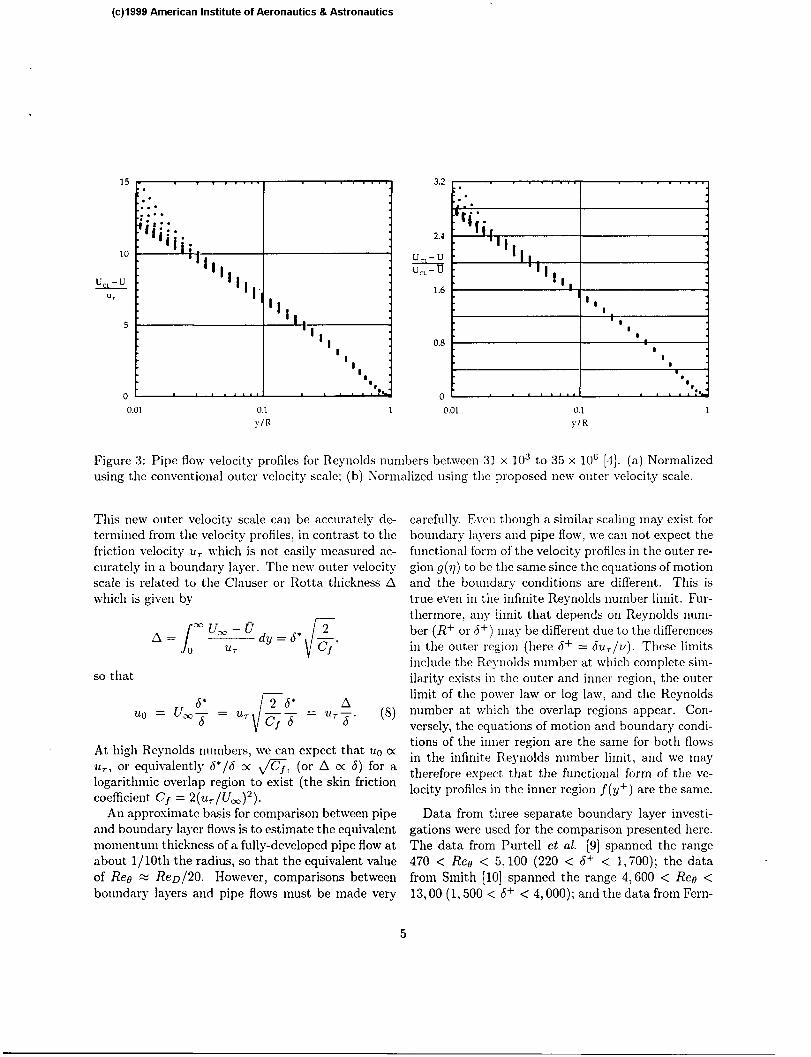
For the preceding argument to be valid, ~0 must bc proportional to U, at high Reynolds number. The correct velocity scale for the outer region was shown to bc the velocity deficit in the pipe, or UC, - i?, where l? is the average velocity, which is a true outer velocity scale, in contrast to the friction velocity which is a velocity scale associated with the inner region which is Ymprcssed” on the outer region [4]. The comparisons with the data arc shown in figure 3. As expected on the basis of the argument given here, the collapse of the data for y/R > 0.1 using uo is considerably better than that using IL,.

4 Turbulent Boundary Layers The preceding analysis for pipe flow may also hold for boundary layers if the centerline velocity is replaced by the freestream velocity and the radius is replaced by the boundary layer thickness [8]. Here we also assume that the streamwise dependence of the velocity profile is properly accounted for by our choice of length and velocity scales. An outer velocity scale equivalent to UCL - u can be expressed using boundary layer parameters as follows.

uo =

I I


Diffuser section

1.3 m l-n n-l 1

I’uniping section Heat exchanger

l-&turn leg

Figure 1: Tllc layout of tllc SupcrPipc facility. The flow direction is counter-clockwise.

10’ Y*

ld IO4 --ld 10’ Y-

10’ Id

Figure 2: Pipe flow velocity profiles normalized using inner scaling variables for 26 different Reynolds twilbers between 31 x lo3 to 35 x lo6 [4]. (a) Log-log plot; (b) Linear-log plot.

4


15

10

u,,-u

“7

5

0

c . .

. . .

. . . . a.

Iriiji.,

il.

'II,

' II'

"I, I

'11 I

'5 I .

'a I;

0.01 0.1 1 )IR

0.01 0.1 1 y/R

Figure 3: Pipe flow velocity profiles for Reynolds numbers between 31 x lo3 to 35 x 10” [4]. (a) Normalized using the conventional outer velocity scale; (b) N ormalized using the proposed new outer velocity scale.

This new outer velocity scale can be accurately dc- termined from the velocity profiles, in contrast to the friction velocity or which is not easily measured accurately in a boundary layer. The new outer velocity SC& is related to the Clauscr or Rotta thickness A which is given by

so tl1at

6’ WJ = urn- = 21,

d

2 6’ A -- = 6 Cf 6 u,-. 6 (8)

At high Reynolds mmrbers, we can expect that ILO cx Us, or equivalently 6*/S K fl, (or A 0: S) for a logarithmic overlap region to exist (the skin friction coefficient Cf = ~(u~/U~)~).

An approximate basis for comparison between pipe and boundary layer flows is to estimate the equivalent momentum thickness of a fully-developed pipe flow at about l/lOth the radius, so that the equivalent value of Ree z ReD/20. However, comparisons between boundary layers and pipe flows must be made very

carefully. Even t.hough a similar scaling may exist for boundary layers and pipe flow, we can not expect the functional form of the velocity profiles in the outer region g(n) to be the same since the equations of motion and the boundary conditions are different. This is true even in the infinite Reynolds number limit. Fur- thcrmore, any limit that depends on Reynolds number ( Rf or S+) may be different due to the differences in the outer region (here S+ = 671,/v). These limits include the Reynolds number at which complete similarity exists in the outer and inner region, the outer limit of the power law or log law: and the Reynolds number at which the overlap regions appear. Con- versely, the equations of motion and boundary conditions of the imler region are the same for both flows in the infinite Reynolds number limit, and we may therefore expect that the functional form of the velocity profiles in the inner region f(y+) are the same.

Data from three separate boundary layer investi- gations were used for the comparison presented here The data from Purtell et al. [9] spanned the range 470 < Ree < 5: 100 (220 < S+ < 1,700); the data from Smith [lo] spanned the range 4,600 < Ree < 13,00 (1,500 < Sf < 4,000); and the data from Fern-

5

(c)l999 American Institute of Aeronaut& & Astronautics

holz et al. [42] provided the data at Ree = 21,000 and 58,000 (S+ = 6,900 and 18,000). I

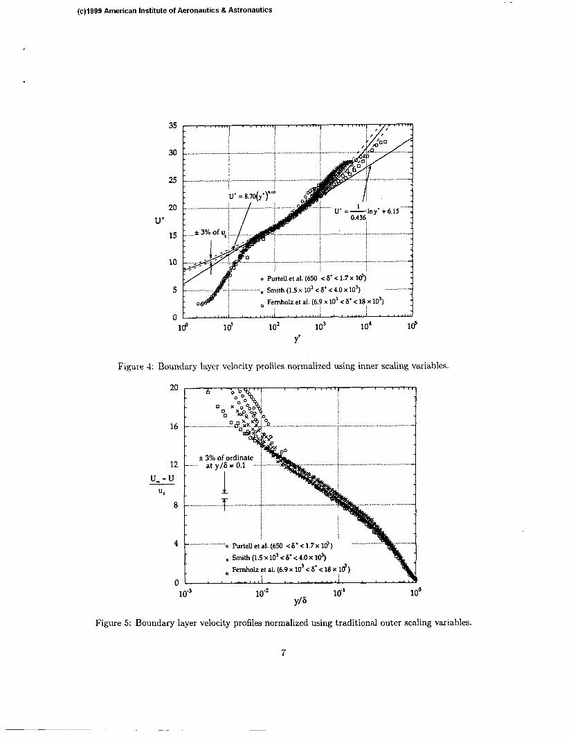
1 In figure 4, the velocity profiles reported in [9], [lo] and [42] are shown normalized by inner layer variables. The data at values of S+ < 500 are not shown since it is doubtful that a universal overlap region exists at these Reynolds numbers. The power law es- tablished from pipe flow data is also shown, as are the regions marking a &3% error in u., (represent- ing a best estimate for the uncertainty in u,). For all profiles except at the highest, Reynolds number, the data arc nominally within 13% of the power la\{ for some range of y+ and deviate from the curve in the inner region where viscosity dominates and in t,he outer region where the inner scaling no longer holds. At the highest Reynolds number: the data near the tvall deviates from the other profiles by more than 3%, but this perhaps can be attributed to an error in position since the five points ncarcst to the wall dre all within 1 xnxn of the wall. The log law estab- lished from pipe flow data is also shorvx~ in figure 4. According to the analysis of pipe flow data, the log law should be apparent only at the highest Reynolds number since a log law should not. exist until S+ is of order 10”. The uncertainty in the friction velocity &events us from drawin g any definitive conclusions hcrc, but a power law with Cl = 5.70 and y = 0.137 swxns to be in good agreement. with these boundary liiyer d;ttEl.

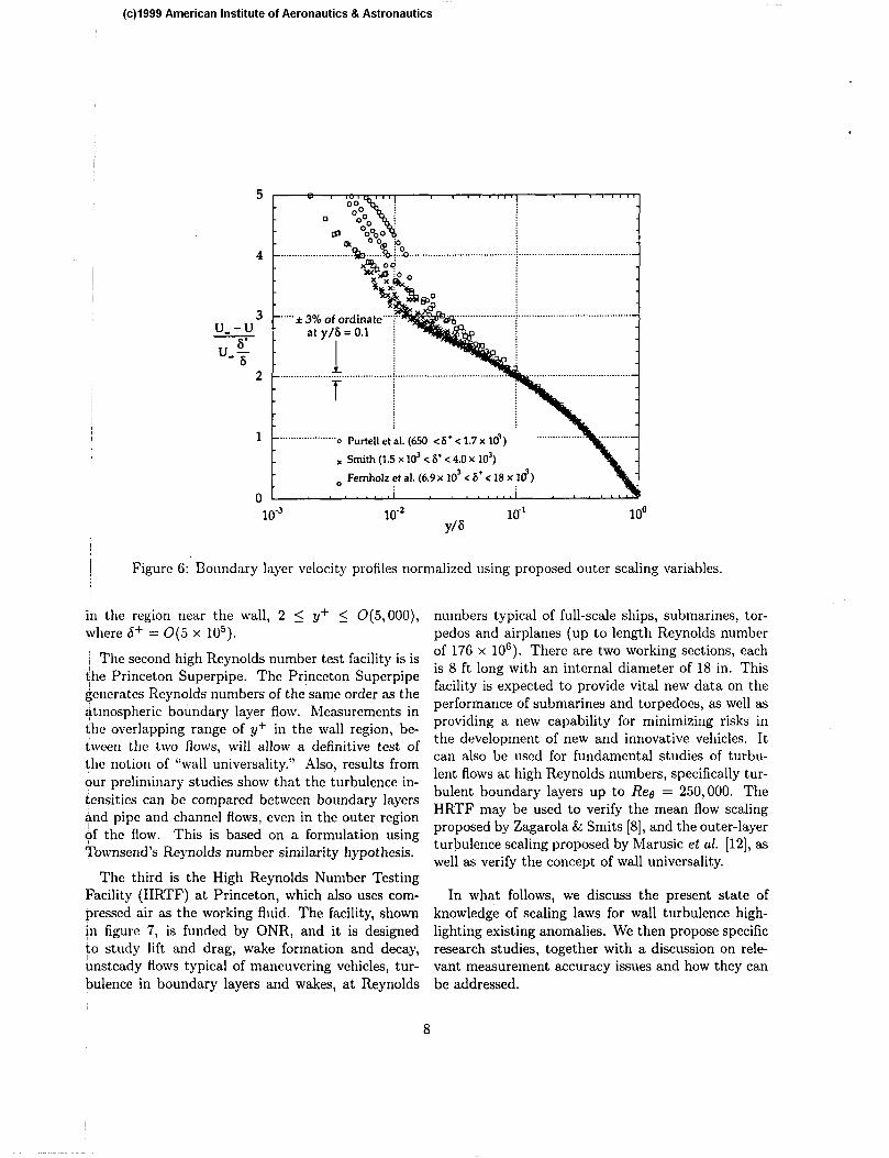
In figures 5 and 6, the velocit,y profiles are nor- malizcd by the conventional out,er velocity scale, ur, and the proposed outer velocity scale U,S*/S, respectively. In each figure, error bars are shown which rcprcsent a f3% uncertaimy of the ordinate at y/S = 0.1. When normalizing the wall-normal position in the outer region, the length scale was taken to be the boundary layer thickness at 0.99U,, although it was found that the profiles collapsed equally well &hen using the displacement thickness or momentum t$ckness. Regardless of the length scale used, the collapse is poor in the outer region for the profiles normalized by u, and much improved for y/S > 0.07 kd for 650 < S+ < 18 x lo3 when using U,S*/S.

I 6

5 Turbulence Scaling Many existing turbulence modeling schemes rely on

the assumption of wall functions, where the turbulence intensities follow the mean-flow behavior and scale with inner-flow variables. That A, where U/U, = g(y+) is approximately valid, UT/~: = fi [y+], 2/u”, = fz[y+], z/u’, = fs[y+]; and so forth. Here U is the mean streamwise velocity, ~1, u2 and ug are the streamwise (x), wall-normal (y) and spanwise (2) components of the fluctuating velocity respectively and overbars denote temporal averages.

A large mmlber of studies have now emerged which strongly contest such thinking. In line with this, Marusic et al. [12] proposed a similarity law for the streamwise turbulence intensity which predicts that the level of 3/u: should increase monotonically with increasing Reynolds number, in the turbulent wall region, e.g. for say, y+ > 100; y/S < 0.15.

Esisting experimental data show support for this formulation which is consistent with Townsend’s attached eddy hypothesis. However, these studies have all been at conventional laboratory scales and it is unclear whether or not this formulation is valid at very high Reynolds numbers and to what limit this idea can be extended. For the other components of Reynolds stress (2,2, - -uiuz) the Reynolds number scaling issue remains even more unclear.

To address these issues, and the structure of high Reynolds number wall turbulence in general, the need clearly exists for high quality turbulence measurements in high Reynolds number boundary layers. By ‘high! we mean S+ = 0( 105), where S+ = 6+/v.

There is an urgent need for research to quantify, in precise terms, the Reynolds number scaling laws for the Reynolds stress tensor uiuj in canonical turbulent boundary layers. To achieve this, three unique and complementary high Reynolds number facilities are now available, which together can provide a com- pletc picture of the wall turbulence across the entire layer. The first is in the atmospheric boundary layer on the salt-flats of Utah at the SLTEST facility. The SLTEST (Surface Layer Turbulence and Environ- mental Science Test) facility provides an environment suitable for mimicking wind tunnel-like conditions. This facility can provide high accuracy measurements


U' 20 ______....___........... i _.......... /r . . . . . . . . . . . . . i . . . . . . :.J

Boundary layer velocity protilcs normalized using inner scaling variahles.

16

A 3% of ordinate ! 12 u--u

", 8 f j

. . . . . . . . . . . . . . . . (. . . . . . . . . . . . . . . . . .

““““““““““a PurteU et II. (650 c6* < 1.7 x ld)

lo”

x smith (1.5 x lo3 c 6’ c 4.0 x 103)

D Fernholz et al. (6.9 x 103 < 6* c 18 x ld) I I

lo’* l(T' Y/6

Figure 5: Boundary layer velocity profiles normalized using traditional outer scaling variables.

7


5

4

““““““““““‘o Purtell et al. (650 <S’ c 1.7 x ld) . . . . . . . ?

x Smith (1.5 x 10’ < 6’ c 4.0 x 10’)

D Femholz et al. (6.9 x IO’ c 6’ c 18 x Id)

lo'* 10-l Y/6

Figure 6: Boundary layer velocity profiles normalized using proposed outer scaling variables.

in the region near the wall, 2 2 y+ 2 0(5,000), where 6+ = 0(5 x 105).

~ The second high Reynolds number test facility is is the Princeton Superpipe. The Princeton Superpipe generates Reynolds numbers of the’same order as the atmospheric boundary layer flow. Measurements in the overlapping range of y+ in the wall region, between the two flows, will allow a definitive test of the notion of “wall universality.” Also, results from our preliminary studies show that the turbulence intensities can be compared between boundary layers and pipe and channel flows, even in the outer region of the flow. This is based on a formulation using Townsend’s Reynolds number similarity hypothesis.

The third is the High Reynolds Number Testing Facility (HRTF) at Princeton, which also uses compressed air as the working fluid. The facility, shown in figure 7, is funded by ONR, and it is designed to study lift and drag, wake formation and decay, unsteady flows typical of maneuvering vehicles, turbulence in boundary layers and wakes, at Reynolds I

numbers typical of full-scale ships, submarines, tor- pedos and airplanes (up to length Reynolds number of 176 x 10’). There are two working sections, each is 8 ft long with an internal diameter of 18 in. This facility is expected to provide vital new data on the performance of submarines and torpedoes, as well as providing a new capability for minimizing risks in the development of new and innovative vehicles. It can also be used for fundamental studies of turbulent flows at high Reynolds numbers, specifically turbulent boundary layers up to Ree = 250,000. The HRTF may be used to verify the mean flow scaling proposed by Zagarola & Smits [8], and the outer-layer turbulence scaling proposed by Marusic et al. [12], as well as verify the concept of wall universality.

In what follows, we discuss the present state of knowledge of scaling laws for wall turbulence high- lighting existing anomalies. We then propose specific research studies, together with a discussion on rele- vant measurement accuracy issues and how they can be addressed.

8


PRINCETON / ONR High Reynolds Number

Test Facility

Figure 7: The High Reynolds Number Testing Facility at Princeton University.

6 Scaling Laws for Wall Turbu- lence

In recent reviews of esperiment.al data, there has been considerable discussion on the applicabiliby of scaling laws to the streamwise t.urbulence intensity (q). (Limited discussion of other turbulence quantities is probably due to the shorbagc of reliable measurements). Gad cl Hak S: Bandyopadhyay[l3] and Fern- holz & Finley (141 icvicwcd zero-pressure-gradient turbulent boundary layers and noted evidence of strong Reynolds number effects on 3 when normal- izcd using inner-wall variables. By inner scaling WC nican q/,(15 = f[y+] while outer scaling involves nor- malization with the lcngtli scale b. Mochizuki & Nieuwstadt [ 151 surveyed a large collection of experimental data in both conventional flat plate boundary layers and in pipes and ducts and slccific attention was given to whether the peak in UT, which occurs at y+ x 15, is Reynolds number independent. Varia- tions between different experiments of this value for T/u: were *lo% but the variation was concluded not to bc statistically significant. Coles [16] also surveyed a large numbers of wall-bounded flow experiments and arrived tentatively at the same conclusion.

Fernholz & Finley [14] suggest that a weak Reynolds number effect may be present but like Coles: draw attention to the difficulty of reaching firm conclusions in the presence of the significant scatter in the data. Mochizuki S: Nieuwstadt further concluded that T does scale with inner-flow variables in the entire wall region (we understand this to be from y+ = 0 to y/S < 0.15, say) which agrees with the approach t.aken by many conventional computational turbulence models where the existence of inner-layer scaling is assumed for all components of the Rcynolcls stress tensor and mean-flow velocity. Smits 5: Dus- sauge [17] ancl Dussauge et al. [18] also reviewed the data presented in [14] and arrived at the conclusion that for a high enough Reynolds number the T profiles display similarity in the viscous sublayer and buffer layer in inner scaling, while similarity in outer scaling is observed in the mean-flow logarithmic layer and the remainder of the outer region.

Doubts as to the validity of inner-flow scaling in the near-wall region have recently been raised in [19] and [20] from studies of computational DNS results. Durst et al. [21] made LDA measurements in a low- Reynolds-number pipe flow and also concluded that turbulence intensities in the wall region do not scale with inner variables. However, they note that very

9

close to the wall only a weak Reynolds number de- dendence exists. For y+ < 15 they believe their data, within experimental uncertainty, scales with in- her variables.

! Marusic et al. [12) proposed a similarity law for 3 for zero-pressure-gradient wall turbulence, formu- lated for the region of the flow above the viscous buffer zone, that is, y+ > 100 and y/b 5 1. The formulation is based on the attached eddy hypothesis, $s extended by Perry & Marusic 122) and ‘Marusic & Perry [23) and the Reynolds-number-similarity hy- dothesis [24). A further assumption is made of the existence of Kolmogorov eddies wjth a universal in- ertial subrange. The form of the expression is

u2, - Al ln[;] - IQ/+] - WJ;], (9)

$here Al and B1 arc universal constants (for full) developed zero pressure gradient layers), 1% is a cor- rkction term for t.he Kohnogorov and attached eddy Jut-off where 1; + 0 for y+ sufficiently large and 14$ is a term analogous to the me;!n flow Coles wake function where IV, + 0 for 2//6 sufficiently small. This is shown schematically in figure 8. In figure 9, a comparison between existin g experimental data and t!hc formulat,ion is shown and good agreement is ob- &n:ed. Also shown on t.his figure is the predicted brofilc for b+ = ~u,/v = 5 x 10’. This is the range of &eynolds number that will be con8idered in the proposed research. Going to sucl~ a high Reynolds num- bcr should provide a definitive test for equation 9.

The most significant implication of equation 9 is that the lc~cl of q/u: at y+ = 0(200), say, con- $nues to rise with Reynolds number without limit. T&is trend implies that with increasing 6+ then (u~/U’),+=,,, (where U is the local mean velocity) <vi11 increase without limit. This ultimately must I’cad to momentary flow reversals occurring. At first glance, it would appear that the formulation might “self destruct” at sufficiently high Reynolds numbers because of this. Nevertheless, from work by Perry & Chong (251 which considers the flow topol- bgy of turbulent boundary layers near the wall, mo- Lientary flow reversals were shown to occur even in ihc zero-pressure-gradient flow case [26], at least at


10

yf ---* 0. These observations come from studying streamline and vortex line patterns. The same work also shows that in adverse-pressure-gradient layers, such momentary flow reversals in localized regions are very common, as seen in the data of [27], at least at y+ + 0, even though the flow in the mean is attached. It could well be that the similarity law is still valid even with such flow reversals. In the absence of high Reynolds number measurements, how far this formulation can be extended is not known.

6.1 Implications for near-wall region The other striking feature of the 6+ = 5 x 10” prediction is that the level of T/U: exceeds the peak turbulence intensity at y+ x 15. In such an event, it is difficult to see how inner-flow scaling could be valid for q. The implications of scaling trends for the other components of turbulence intensity can also be considered using the attached eddy hypothesis, which is main theory behind equation 9. For example, in the case of the wall-normal componet (3): the attached eddy hypothesis would imply that +2, remains invariant with Reynolds number in the wall-region. The explanation behind this is also related to the notion of “inactive motions” as discussed in [28] and [29]. These are large-scale motions which contribute to the streamwise and spanwise broadband-turbulence intensities near the wall but not the wall-normal turbulence intensity and Reynolds shear stress. Townsend (291 points out that these “motions” can be fully described by the presence of attached eddies and this is incorporated in the attached eddy model of [22]. Here the main energy-containing motions of the boundary layer are described by superimposing the contributions from a range of scales of geometrically similar represen- tative eddies, and the contribution of one scale of eddies of length scale 6, to T/U: is proportional to Ill[y/&], the streamwise Townsend eddy intensity function. By Taylor series expanding the velocity field for inviscid boundary conditions, Townsend [30] deduced that 111 must approach a constant as y/6, ---t 0, whereas it rapidly decays to zero for increasing y/b, for y/a, > 1. This directly implies that all eddies with length scale 6, > O(y) will have con-


Figure 8: .4 mean-flow velocity-defect analogous picture for the streamwise broadband-turbulence intensity for flow irl~~v(: the viscolls buffer zone (!I+ 2 100).

SLTEST Range - R,= 1410Spahn J 44 0 = 2190 Mclean I

, Superpipe Range 0 = 4140 Uddin b = 7080 Mclcan 1 -

= 10290 Mclean 0 = 13052 Smith 0 =20920DNW A = 35100 Petrie V = 57720 DNW

Figure 9: Similarity equation 9 (solid lines) compared to zero pressure gradient boundary layek data (taken from Marusic et al. 1997), and prediction for 6 + = 6 U,/V = 5 x lo5 as expected for SLTEST and Superpipe flows.

11


tributions to T/a: at this y-position and this results in the “inactive motions.” This also applies to the h- tensity function 133[y/&], and hence uz/u”,, the span- \yise intensity. This is not true for 122 and 112 which fall to zero as y/b, + 0. As the Reynolds number ihcreases,the range of eddy length scales 6, increases and so UT/$ and z/u: keep increasing but q/u: ahid -e/L: asymptote to a finite universal limit 4bove the buffer zone. (It is important to restate that this only applies for the region above the viscous l&ffcr zone where inviscid boundary conditions apply and the motions can be thought of as a “meandering and swirling” of the fluid in the streamwise-spanwise filane).

Considering these trends, it would seem reason- &le to speculate that the influence of these “inactive motions” is the following. Since the intensities -77 u-/us and q/l+ I1

’ increase with increasing Reynolds mmibcr, above the buffer zone, it is likely that these components will 7~0t show inner scaling in the viscous slublayer and buffer zone. Conversely: since z/u: dnd -YL~~u~/$ retain universal values invariant with yf for y/c5 + 0 above the buffer zone for increasing Reynolds numbers, it is likely that these quantities will show inner scaling in the viscous sublayer and buffer zone. ~ The above predictions are not likely to be valid if

the R.eynolds mmlber is not sufficiently large, since the ratio of the largest to smallest attached eddies $4 proportional to S + = Su,/u. Restricting measure- l~icnts t,o lo~v-Reynolds-number flows may mean that an inadequate range of scales of attached eddies exists. This is probably the case for the low-rteynolds- number data reviewed by Bradshaw S: Huang [19] where they concluded that none of the Reynolds stresses show inner-scaling. Experiments at very high &cynolds numbers are needed to resolve the issue.

9.2 Anomalies in existing data

The debate over the correct Reynolds number scaling for the turbulence intensities, is further exacer- bated by preliminary measurements of streamwise turbulence intensity which have been carried out in the Princeton Superpipe [31], [32]. The data appear to show an anomalous behavior, where at Reynolds

numbers greater than 500,000, the turbulence intensity (scaled according to conventional wisdom) at a given distance from the wall decreases with Reynolds number. If this behavior is indeed correct, it indicates a completely new scaling, contrary to conventional wisdom and the scaling predicted by the attached eddy hypothesis. Since there are no other pipe flow data (nor boundary layer data) at higher Reynolds numbers to verify this result, it stands or falls on the accuracy of the measurements. Two sources of possible error exist: the spatial resolution of the probes (which would tend to reduce the measured turbulence intensity) and the fact that the flow may not be fully-developed (even with L/D = 150) at the highest Reynolds numbers. Clearly, further experiments are needed and the complementary measurements in the SLTEST and HRTF facilities could provide the necessary comparison to the Superpipe data.

Preliminary measurements have also been carried on the Ut.ah salt flats prior to the development of the SLTEST facility ((331, [?I) and these results indicate that T/,,,: increases with Reynolds number in the turbulent wall region. However, significant scatter is observed in these early field tests, probably due to an insufficient nuxriber of realizations being obtained under difficult field conditions. recent improvements to the SLTEST facility, which was developed under an NSF Infrastructure Grant, allow more suitable conditions for accurate measurements with greatly improved on-site calibration facilities.

6.3 Outer-scaling in internal flows In figure 9 an indication was given of the experimental range that each the SLTEST and Superpipe can cover. (These ranges have been estimated in order to obtain accurate hot-wire measurements. A mea- suring range of approximately 1 mm 5 y 5 1.5 m is assumed for the SLTEST flow and approximately 0.5 mm 2 y < (63.5 mm = 6) for the Superpipe). In this way, it is seen that experiments in both facilities are required in order to give a complete picture of the wall turbulence. Clearly, it will be possible to evaluate the scaling law trends with these proposed experiments. However, for a quantitative comparison to be made between the turbulence intensities


(4 0 Pipe: Kr = 3900. Henbest (1983) 0 Pipe: K, = 1610. Henbest (1983) A Channel. K, = 1655, Wei & Willmnrrh (I 989) n Channel. K, = 8160, Comte-Bellor (1965)

-... -a..

--. ‘-.. K,= 6+ =5x105 1

*... 1

12 , , I

t (b)

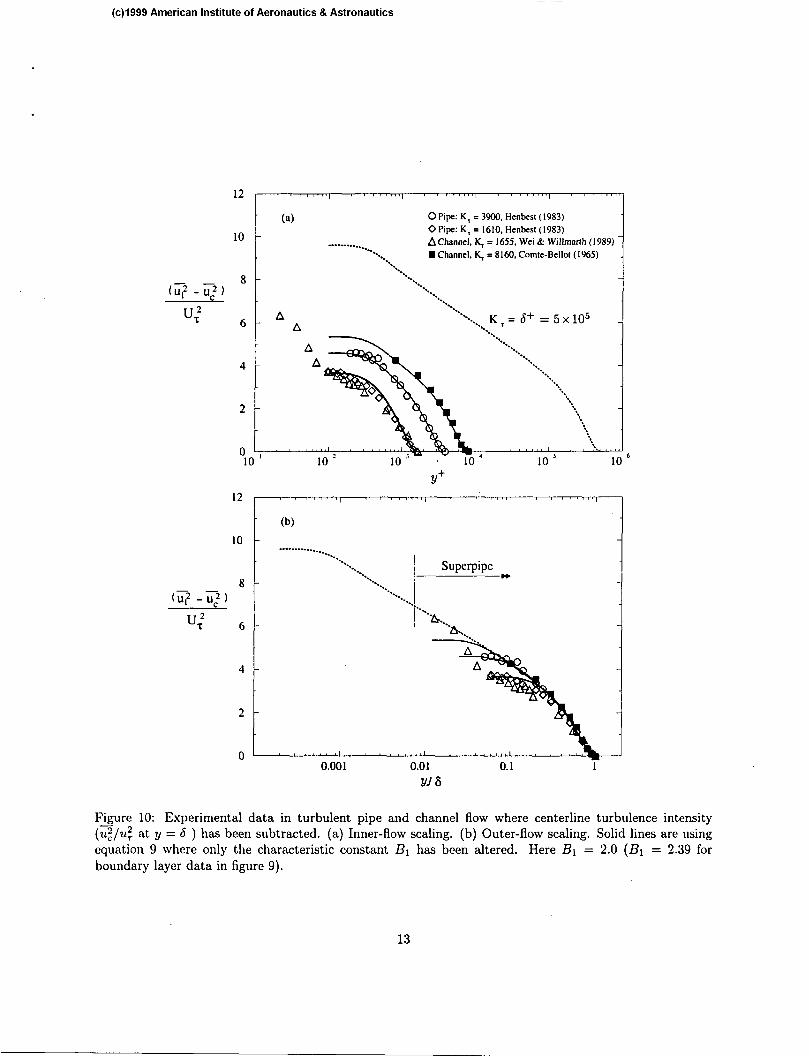
Figure 10: Experimental data in turbulent pipe and channel flow where centerline turbulence intensity (2/u: at y = b ) has been subtracted. (a) Inner-flow scaling. (b) Outer-flow scaling. Solid lines are using equation 9 where only the characteristic constant B1 has been altered. Here B1 = 2.0 (B1 = 2.39 for boundary layer data in figure 9).

13

(c)l999 American Institute of Aeronautics 81 Astronautics

oif the two flows in the outer part of the flow, some further rationale is required. Some preliminary work on this issue suggests that should be possible. The obvious difference between an unrestricted boundary layer flow, such as in the SLTEST facility, and a fully- +veloped flow, as found in pipesand channels, is that a+ the edge of the layer y = 6, uf = 0 in the boundary layer while 3 is finite (equal to 2 say) for the $ipe or channel (here b is the pipe radius or channel half-width). Our preliminary results show that sub- tracting off the centerline turbulence intensity gives a favorable agreement with the original similarity equation 9, as shown in figure 10. As indicated, these re- s;ults are of a preliminary nature: although they seem encouraging. I I

7 Measurement Accuracy Is- sues

Ik previous reviews [14], [35]? [15], existing esperi- mental data for 2, and where available z? 2 and --zL~~L~ show a large degree of scatter! reflecting the problems of measurement accuracy in these flows. This makes it ahnost impossible to draw firm conclusions about Reynolds number scaling, especially given the restricted range of ReynGlds numbers con- slidered. Going to very high Reynolds numbers will dcrtainly resolve the qualitative trends, provided the mcasurcment errors arc not excessive. However: in order t.o quantify this Reynolds mmlber dependence it is essential to address two major measurement ac- cllracy issues. The first rclatcs to spatial and tem- ioral resolution issues and the second to calibration broccdurcs.

7.1 Spatial and temporal resolution

Inaccurate measurement of turbulence intensities will result when the length of the sensing element of the hot-wire is larger than the length scales of motion {vhich contribute to the turbulence intensity. Sim- ilarly, if the sampling rate is not sufficiently fast, energy contribut,ions will be missed from turbulence scales ,associated with frequencies larger then half the

masimum sampling rate (based on Nyquist’s sampling criterion).

One of the main advantages of the SLTEST boundary layer is the extraordinary large scales which will be encountered. The Kolmogorov length scale, 77 is estimated’ to be O(l mm) near the wall which is of the same scale of conventional hot-wire filaments. In addition, the frequencies that need to be resolved at non-dimensional wavenumber, k1~ = 1, correspond to O(lOO0 Hz)~. Therefore there will be no difi- culty in resolving the turbulence fully with conventional techniques and no need to make any a priori assumptions such as isotropy of the high wavenumber motions. Correction schemes, such as that of Wyn- gaard [3G] have been used extensively but up to now there h,as been no way to test the assumptions rig- orously. These correction schemes may be tested in the SLTEST flow, and a new experimentally-based high-~~.a\relluinber correction scheme can bc developed. The additional advantage of this correction scheme is t.hat it will be obtained in a Aow where there is no “f2 noise” as discussed in [37]. This noise problem relates to conventional hot-wire anemome- ters and appears to be prevalent at high frequencies where low signal-t.o-noise ratios are present.

In the Superpipe and HRTF measurements, spatial and temporal resolution limitations will be a major issue. Here, the Kolmogorov length scale is estimated to be O(2LLm) at y = 1 mm while at Ic1~ = 1, frequencies are estimated to be 0(2 MHz). Using ultra-fast data acquisition hardware (sampling rate > 2 MHz) and sub-miniature probes 1 = O(O.l mm) will help reduce the extent of the problem, but at some point high wavenumber corrections will need to be implemented. This is where the correction scheme obtained from the SLTEST results will be important.

7.2 Low-speed calibration

In the SLTEST measurements, low velocities are encountered close to the wall. At a wall-normal distance

lHcre, q4 x v3ny/u3,, using the assumptions that produc- tion and dissipation of turbulent kinetic energy are in balance and that --‘(L~uz x IL’,.

2Frequency is converted to streamwise wavenumber using Taylor’s hypothesis of frozen turbulence: kl = 2n f /CJ.

I 14


of 1 mm (y+ % 4) mean velocities of approximately 0.3 m/s can be expected. In this range, corrections are required for both the manometer and the Pitot- static tube. It is important to resolve this issue as it is in the low speed range that hot-wires are most sensitive to velocity perturbations and hence inaccurate calibrations can lead to misleading turbulence intensity measurements.

Hot-wires need to be calibrated relative to a known velocity reference. This is usually done with a Pitot- static tube and a differential pressure transducer. Unfortunately, this technique becomes difficult for velocities less than approximately 1 m/s due to the low levels of pressure difference and in general, even the highest quality pressure transducers will have some non-linear behavior at these low velocities. An additional problem also arises as the Pitot tube reading it,sclf mill require a Reynolds number correct.ion nhcu the Reynolds number based on the tube diamct,cr is below approximately 100 [38].

To overcome thcsc difficulties! the Pit.ot-static and the pressure transducer may bc calibrated as a complete system relative to a ki~ow~ velocity reference. Two previously t.estcd methods can be considered: one is based on a technique developed by Haw 6 Foss [39] and involves having a hot-wire attached to a piv- oted arm falling under the action of gravity. The second method uses a “flying hot-wire:’ facility similar to the one described in [40]. It involves mounting a hot-wire to an air-bearing sled which moves back and fort.11 in a known sinusoidal motion. In this was the speed and position of the probe are known at all times. The technique relies on the fact that the hot-wire sensitivity has a well defined peak when the velocity of the flow over the wire reaches zero. The tunnel velocit,y is adjust,ed such that on the down- st.ream stroke, and at its mid-position when the sled is at a (negative) maximuiii, the hot-wire is moving at zero velocity relative to the flow. (This can be done by monitoring an oscilloscope trace or by using a digitally sampled signal). The tunnel velocity is then known to be at the same velocity as the sled. This technique was successfully implemented by Tan [41] in a study of low velocit,y free shear flows.

8 Summary

It has become apparent in the last few years that the widely accepted scaling arguments for turbulent wall-bounded flows need to be revised in light of new experimental results and new analysis. At the same time, new facilities have become available (for example, the Princeton Superpipe and HRTF facilities, and Utah’s SLTEST facility), which offer a very large range of Reynolds numbers where new scaling concepts can be tested. Based on the current understanding of turbulent flows, we have tried to suggest cxperimcnts that make use of these new facilities to improve our understanding of the basic scaling laws of turbulent flows. This will provide more rigorous methods for extrapolating model results to the full scale prototype with greater accuracy.

Acknowledgments

The research in high Reynolds number flows is sup- ported by ONR through grants N000014-97-l-0618, DURIP/ONR G rant N00014-98-1-0325, and N00014- 99-I-0340, monitored by Drs. C. Wark and L.P. Purtcll.

References

[l] George, \V.I<., Castillo, L., and Knccht, P. 1996. The zero pressure-gradient turbulent boundary layer. Technical Report No. TRL-153, S.U.N.Y. Buffalo.

[2] Barenblatt, G. I., Chorin, A J., Hald, 0. H. and Prostokishin, V. M. 1997. Structure of the zero-pressure-gradient turbulent boundary layer. Proc. Natl. Acad. Sci, USA, 94:7817-7819.

[3] Zagarola, htI.V. and Smits, A.J. 1998. Mean-flow scaling of turbulent pipe flow. J. Fluid Mech., 373, 33-79.

[4] Zagarola, M.V. and Smits, A.J. 1997. Scaling of the mean velocity profile for turbulent pipe flow. Physics Review Letters, 78 (2), 239-242.

15


Schlichting, H. 1987. Bounday-Layer Theory. McGraw-Hill.

hflillikan, C.M. 1938. A critical discussion of turbulent flows in channels and circular tubes. Proc. 5th Int. Congr. Appl. h/lech., Wiley.

Zagarola, M.V. 1996. Mean flow scaling in turbulent pipe flow. Ph.D. Thesis, Princeton Uni- versity.

Zagarola, M.V. and A.J. Smits, A.J. 1998a. A new mean velocity scaling for turbulent boundary layers. AShJE Paper FEDShr198-4950, 1998.

Purtell, L.P., Klcbanoff, P.S. and Buckley: F.T. 1981. Turbulent boundary layers at low R.eynolds number Phys. Fluids, 24 (5), 802-811.

Smith! R.\\‘. 1994. Effect of Reynolds number 0x1 the structure of turbulent boundary layers. Ph.D. Thesis, Princeton University, Princeton, NJ.

Fcrnholz, H. H., Krause, E. Nockcmann, M., and Schobcr, h/I. (1995. Comparative measurements in the canonical boundary layer at Res 5 G x 10’ on the wall of the DN\V. Phys. Fluids, 7:1275- 128!.

Marusic, I., Uddin, A. I<. hl. and Perry, A. E. 1997. Similarity law for the streamwise turbu- lcncc intensity in zero-pressure-gradient turbulent, boundary layers. Physics of Fluids, 9:3718- 3726.

Gad cl Hak! hgl. and Bandyopadhyay, P. R. (1994. Reynolds number effects in wall-bounded turbulent UO\VS. Applied h!echanics Reviews, 47(8):307-365.

Fcrnholz, H. H. and Finley, P. J. (1996. The incompressible zero-pressure-gradient turbulent boundary layer: an assessment of the data. Prog. Aerospace Sci., 32:245-311.

h,lochizuki, S. and Nieuwstadt, F. T. hl. 1996. Reynolds-number-dependence of the maximum in the streamwise velocity fluctuations in wall turbulence. Exp. Fluids, 21:218-226.

16

PGI

P’il

PI

PI

[20]

PI

[22]

PI

WI

PI

PI

Coles, D. (1978. A model for flow in the viscous sublayer. In Proc. Workshop on Coherent Struc- ture of Turbulent Boundaq Layers (Ed. Smith, C. R and Abbott, D. E.), Lehigh University, USA.

Smits, A. J. and Dussauge, J. P. 1996. Turbulent Shear Layers in Supersonic Flow. AIP Press.

Dussauge, J. P., Fernholz, H., Finley, P. J., Smith, R. W., Smits, A. J. and Spina, E. F. (1996. Turbulent boundary layers in subsonic and supersonic flow. AGARDograph 335.

Bradshaw, P. and Huang, G. P. 1995. The law of t,he wall in turbulent flol~. Proc. R. Sot. Lond. -4: 451:165-188.

Moser, R. D., Kim, J. and Mansour, N. N. 1999. Direct numerical simulation of turbulent channel flow up t,o R, = 590. Physics of Fluids, 11:943- 945.

Durst, F., Jovanovic, J. and Sender, J. (1995. LDA measurcmcnts in the near-wall region of a turbulent pipe flow. J. Fluid hlech., 295:305- 335.

Perry, A. E. and Marusic, I. 1995. A wall-wake model for the turbulence structure of boundary layers. Part 1. Extension of the attached eddy hypothesis. J. Fluid Mech., 298:361-388, 1995.

Marusic, I. and Perry, A. E. 1995. A wall-wake model for the turbulence structure of boundary layers. Part 2. Further experimental support. J. Fluid Me&., 298:389-407.

Townsend, A. A. 1956. The Structure of Turbu- lent Shear Flow. Cambridge University Press.

Perry, A. E. and Chong, M. S. 1994. Topology of flow patterns in vortex motions and turbulence. Applied Sci. Research, 53:357-374.

Spalart, P. R. 1988. Direct simulation of turbulent boundary layer up to Re = 1410. J. Fluid hlech., 187:61-98.


1271 Spalart, P. R. and Watmuff. J. H. 1992. Ex- [39] H aw, R. C. and Foss, J. F. 1990. Facility for low perimental and numerical study of turbulent speed calibrations. ASh4E, Proc. Symp. Heuris- boundary layers with pressure gradients. J. Fluid tics of Therm. Anem., FED vol. 97, University Mech., 249:271-298. of Toronto, 29-33.

1281 Bradshaw, P. 1967 The turbulence structure of 1401 Perry, A. E. 1982. Hot-wire AnernometnJ. equilibrium boundary layers. J. Fluid Mech., Clarendon Press, Oxford. 29:625-645. [41] Tan, D. K. M. 1982. PhD thesis, University of

1291 Townsend, A. A. 1961. Equilibrium layers and h;Ielbourne, Australia. wall turbulence. J. Fluid Mech., 11:97-120. 1421 Fcrnholz: H.H., Krause, E., Nockemann? M., and .

1301 Townsend, A. A. 1976. The Structure of Tur- bulent Shear Flow. Vol.2, Cambridge University Press.

Schobcr! RI. 1995. Comparative hrIeasurements in the canonical boundary layer at Reas < 6 x 10“ on the wall of the German-Dutch Windtunnel. Phys. Fluids: 7 (6), pp. 1275-1281.

[31] Schmanske, h,I. 1999. Turbulence hfeasurements in High Reynolds Number Pipe Flow. h!ISE Thc-

[43] George, W. K. and Castillo, L. (1997. Zero-

sis, Princeton University. pressure-gradient turbulent boundary layer. Ap- plied hdech. Re,views, 50:689-729.

[32] \\‘illiams: D.R. 1998. Oganired Structures in the O,uter Region of a Turb,ulent Pipe F1o.w. h/ISE

[44] h,IcLenn, I. R. 1990. The near wall eddy struc-

Thesis: Princeton University. ture in an equilibrium turbulent boundary layer. Ph.D. thesis! University of Southern California,

[33] Klewicki, J. C. and hktzgcr, RI. Ri. 199G. Vis- USA.

cous wall region structure in high and low [45] Panofsky, H. and Dutton, J. 1984. Atmospheric Reynolds mmlber turbulent boundary layers. Turbulence - Models and Methods for Engineer- AIAA 96-2009. ing Applications. Wiley.

[34] Folz, A., Ong, L. and \Vallacc: J. (1995. Near- [46] Petrie, H. L., Fontaine, A. A., Sommcr, S. T. and wall turbulence measurements in the atmo- Brungart,T. A. 1990. Large flat plate turbulent spheric surface layer. Bull. APS, 40:2027. boundary layer evaluation. Tech. Report TM89-

[35] Srcenivasan, Ii;. R.. 1989. The turbulent bound- 207, App. Res. Lab. Penn. State Univ.

ary layer. In Frontiers in ,Qpeemantal Fluid [47] Uddin, A. K. hf. 1994. The structure of a turbu-

hgechanics, (ed. Gad-el-Hak) 37-61, Springer- lent boundary layer. Ph.D. thesis, University of Verlag. hlelbourne, Australia.

[36] Wyngaard, J. C. 1968. hIeasurements of small scale turbulence structure with hot-wires. J. Sci. Instrum., Series 2, 1:1105-1108.

[37] Saddoughi, S. and Veeravalli, S.V. 1996. Hot- wire anemometry behaviour at very high frequencies. Meas. Sci. Technol., 7, 1297-1300.

[38] Chue, S. H. (1975. Pressure probes for fluid measurements. Prog. Aerospace Sci. 16:147-223.

17

high reynolds number flows: a challenge for experiment...

Documents