19th Australasian Fluid Mechanics ConferenceMelbourne, Australia8-11 December 2014

A Modeling and Simulation Framework for Transonic Flutter Analysis

K. L. Lai1, and K. -Y. Lum2

1Temasek LaboratoriesNational University of Singapore, Singapore

2Department of Electrical EngineeringNational Chi Nan University, Puli, Taiwan

Abstract

The paper presents an approach for flutter prediction usinga combination of full-order computational aeroelastic (CAE)techniques and reduced-order modeling (ROM) methods. Theaeroelastic equations of motion are resolved by using CAE toobtain time-domain aeroelastic responses, upon which ROM isapplied to obtain an aeroelastic reduced-order model in discrete-time, state-space format. The resulting closed-loop aeroelasticmodel is thus analysed for Hopf bifurcation to predict the flut-ter boundaries. The present approach predicts flutter boundariesmuch faster than aeroelasticity simulation, lending it a practicalengineering tool. For application and verification of the method,the benchmark transonic aeroelastic of AGARD 445.6 wing willbe considered. Results show that the present approach predictsaccuately the flutter boundaries.

Introduction

Aerodynamic flutter, an aeroelastic phenomenon caused byclosed-loop interaction between aerodynamic and structural dy-namic, constrains and even poses danger to the operation of air-craft. Flutter prediction is one important process in aircraft de-sign. As an alternative to flight tests, computational aeroelastic-ity (CAE) has become a reliable tool for flutter analysis. Bothlinear unsteady aerodynamics and nonlinear high-level CFDmethods have been developed and applied in CAE. When aero-dynamic nonlinearities such as transonic flutter, shock waves,and high-angle-of-attack problem, the latter are the only meth-ods capable of dealing with the problems.

Because of the high computational cost incurred by full-orderCAE computation, its use for mapping out the flutter bound-aries in the entire flight envelop will lead to excessively longturnaround time. To this connection reduced-order modeling(ROM) techniques have been applied in aeroelastic analysis.ROM can reduce the computational time by several orders ofmagnitude. In general, a reduced-order aerodynamic model isobtained and deployed in lieu of the full-order unsteady flowsolver. Generation of ROM involves two functional steps –generation of training data, and calculation of reduced-ordermodel. Both experimental results and computational results canbe used as ROM training data. The system is subjected to pre-scribed perturbation[1, 2, 4, 9, 10], and aeroelastic responsesare measured and taken as ROM training data. A number of dif-ferent techniques have been developed for calulating reduced-order models. These include Eigenvalue (Modal) Truncation,Balanced Model Reduction, Karhunen-Loeve or Singular ValueDecomposition, System Identification methods, Fourier Seriesmethods, and Hybrid techniques. Dowell and Hall [3] presentsa comprehensive review of recent works. Noor [8] gives someearly examples of model reduction techniques.

In the present work CFD results are used as ROM trainingdata. Full-order CAE simulations are performed to computethe unsteady flows of the non-aerodynamically loaded system

in response to a prescribed perturbation. The staggered phase-modulation signal is applied to prescribe the generalised dis-placement. Each one of the structural modes used is excited atabout its natural frequency and with a phase lag with the preced-ing mode. The staggered inputs method[6] allows training datato be computed in one single run of CAE computation, achiev-ing greater time saving. The present reduced-order modelingtechnique is based on the Hammerstein model and correlationmethod[7]. While the aerodynamic model can be identified byROM, the structural model is identified independently by usingfinite-element analysis. The computed aerodynamic model andstructure model are coupled to form the closed-loop aeroelasticmodel, to which eigen-analysis can be applied to determine theflutter boundaries.

While the CAE techniques and ROM method used in this workwill be briefly dicussed herein, the main focus of this paperwill be on verifying the present numerical scheme. Verificationstudy was performed using the AGARD 445.6 wing. The com-putational aeroelastic results obtained were compared againstexperimental data. The Mach numbers considered correspondto those in the experiments. Computations were performed forflow conditions at two different angles of attack α = 0 and 4.

Modeling of Flutter Dynamics

Aerodynamic flutter is a closed-loop interaction between airflow and flexible structure. The air movement exerts aerody-namic forces on the structure, which reacts by deforming. Thisdeformation results in a time-varying boundary of the flow do-main and, thus, a feedback mechanism between the structuraldynamics and aerodynamics. Figure 1 depicts the schematic ofa closed-loop aeroelastic system. The aeroelastic equations of

Aerodynamic Response

(M∞)

Structural Dynamics

αV2

ModalDisplacements

GeneralizedAerodynamicForces

u=η y=F

fη

Figure 1. Flutter dynamic system.

motion can be expressed in modal coordinates as

ηi +2ζiωiηi +ω2i ηi = fi, i = 1, ...,N (1)

where η is the structure modal or generalized displacement, fthe generalized aerodynamic forces, N the number of structuralmodes, and ζ and ω the damping factor and natural frequency,respectively.

The aerodynamic force vector FFF exerted by the air movement isa nonlinear function of the fluid state vector UUU and the kinematic

boundary conditions as defined by the displacement vector ξξξ ofthe flow domain:

FFF = FFF(

UUU ,ξξξ, ξξξ)

, (2)

whereas the fluid state vector UUU =(ρ,ρvvv,ρE), of density ρ, fluidmomentum ρvvv and total energy ρE, is determined by the solu-tion of the flow governing equation. For this study, the Eulerequation is employed for modeling three-dimensional inviscidunsteady flow, which can be expressed in integral form as

∂∂t

Z

Ω(t)UUU dΩ+

Z

∂Ω(t)F ·nnndσ = 0, (3)

where F is the flux vector, Ω(t) is the flow domain with bound-ary ∂Ω(t), and nnn denotes the outward normal vector on theboundary. The flow domain and its boundary are time-varyingdue to structural deformation. The relation between ξξξ and ηηη isdetermined by a mapping Φ : ξξξ = Φηηη, called the fluid-structurecoupling, which transforms modal displacements into flow do-main displacements. Hence, one can write:

Ω(t) = Ω(ηηη(t)), ∂Ω(t) = ∂Ω(ηηη(t)). (4)

The numerical methods employed for solving the system ofequations (2) – (4) consist of a Cartesian grid-based Eulersolver using a time-accurate second-order implicit scheme andmultigrid procedure to accelerate convergence, and an algebraictransformation for the fluid-structure coupling operator [5]

Equations (2) – (4) describe the aeroelastic response as an N-input, N-output system, with the input being the modal dis-placements ηηη, and output being the aerodynamic forces FFF inmodal coordinates. Solution is obtained at a given free-streamMach number M∞. The generalized aerodynamic force vectorfff acting on the structure is related to FFF by

fff = αV 2FFF (5)

where α is a constant depending on the dimensions and mass ofthe wing, and V is the speed index given by

V =V∞

bsωα√

µ, (6)

where V∞ is the free-stream velocity, bs is the semi-chordlength, ωα is the natural frequency of wing in first uncoupledtorsion mode, and µ is the wing-air mass ratio. The smallestvalue V f of V such that the closed-loop is unstable is called theflutter speed index, and the frequency ω f of oscillation is theflutter frequency. The traditional definition of flutter boundariesare thus the graphs V f (M∞) and ω f (M∞) [11].

Hammerstein Reduced-Order Model for Flutter Dynamics

The above dynamical system of aeroelastic response has no an-alytical model, and flutter analysis by full-order simulation iscomputationally expensive. A faster, system-theoretic methodconsists in obtaining a reduced-order model of this system.Since aerodynamic response can be regarded as weakly nonlin-ear under small modal displacement, the Hammerstein model isa suitable choice for ROM.

The ROM technique used in the paper is based on theCorrelation Method for Hammerstein System Identification(CMHSI)[7]. Reduced-order aerodynamic model is obtained byidentification of the Hammerstein model parameters using inputand output data computed in full-order CAE computations. TheHammerstein model is composed of a static nonlinearity N [·]

followed by a linear block represented by its impulse responsefunction h(τ), as shown in figure 2, where the nonlinearity N [·]is assumed to take an odd-polynomial form,

y(t) = h(τ)∗ x(t)= h(τ)∗N [u(t)]

= h(τ)∗ [γ1u(t)+ γ2u3(t)+ · · ·+ γpu2p+1(t)]. (7)

N[⋅] h[τ]

u x y

Figure 2. Hammerstein model for aerodynamic response.

Determination of Flutter Boundary via Closed-Loop Eigen-value Analysis

By adopting the ROM approach, the flutter dynamics of figure 1is approximated by a closed loop formed by the HammersteinROM and the structure model. As aerodynamic is parametrizedby free-stream velocity and attack angle, a ROM is obtainedfor each flow condition. Thus, at each Mach number M andattack angle α, an (M,α,V f )-parametrized closed-loop modelcan be constructed. Here, the linear structural dynamics arerepresented by their transfer-function matrix Gs(s).

For a fixed flow condition defined by M and α, the onset offlutter corresponds to the appearance (if any) of a limit cycledue to bifurcation as the remaining parameter, the speed indexV f , varies. To determine the condition of limit cylce, the Hopfbifurcation theorem states that:

Theorem 1. For a one-parameter family of nonlinear differen-tial equations x = fµ(x), there exists a limit cycle for µ > µ0 if apair of eigenvalues of the linearized equation at its equilibriumcrosses the imaginary axis from the left-half complex plane tothe right-half.

γ1

Gs(s)

hM ( τ )

u=η x

fηαVf

2

y

Figure 3. Linearized closed-loop model of flutter dynamics.

In the context of the current study, the family of nonlinear differ-ential equations is that of the reduced-order flutter closed loopparametrized by V f . It is important to note that, once the ROMis identified, the closed loop is analytical. Moreover, at zeroequilibrium (u = 0,y = 0), the linearized equation is simply thatof the closed loop with only the linear part of NM , i.e.

x(t) = γ1u(t), (8)

as shown in figure 3. Hence, flutter boundary determinationamounts to calculating V f at which a first pair of eigenvaluescrosses the imaginary axis. This can be easily achieved via linesearch. The crossing frequency is thus the flutter frequency.

Results and Discussion

Computed flutter characteristics of the AGARD 445.6 wing arepresented here. The AGARD 445.6 wing was flutter tested inthe Transonic Dynamics Tunnel, at Mach numbers from 0.4 to1.14 at zero-degree angle of attack. Experimental results[11]from this test have been widely used for computational aeroelas-tic benchmarking. The AGARD wing planform has a quarter-chord sweep angle of 45, an aspect ratio of 1.65, a taper ratioof 0.66, and a symmetric airfoil. The wing model and struc-tural model used in the present work are depicted in figure 4.Five dominant structural modes of the wing, figure 5, are used.Their natural frequencies are

ωi = (60.32, 239.8, 303.8, 575.1, 742.0) rad/sec.

Mode 2 is the first uncoupled torsion mode. That is, ωα =239.8 rad/sec. The structural damping is assumed to be zero,which corresponds to the ’weakened’ 2.5-foot panel-span modeldescribed in Yates[11]. In order to compare with experimentaldata, four Mach numbers are investigated:

M∞ = (0.5, 0.678, 0.90, 0.96).

Y

X

Z

Y

X

Z

(a) Model of AGARD445.6 wing

X

Y

Z

(b) Multi-level Cartesiangrids

Figure 4. Numerical models and computational grids forAGARD wing configuration.

(a) Mode 1, f1 = 9.60Hz

(b) Mode 2, f2 = 38.17Hz

(c) Mode 3, f3 = 48.35Hz

(d) Mode 4, f4 = 91.54Hz

(e) Mode 5, f5 = 118.10Hz

Figure 5. Modal shapes and frequencies of the AGARD 445.6wing (weakened model).

Determination of flutter boundaries using CAE simulation usu-ally follows the bisection approach. Computations are per-formed at different speed indices at a fixed Mach number and at-tack angle. The aeroelastic response in the form of time-varyinggeneralised variables is computed, from which the damping ra-tio is computed using the logorithmic decrement method. Apositive damping ratio signifies stable condition, while nega-tive damping ratio indicates unstable condition. As an exampleof stable flutter response, the computed generalised displace-ment at Mach number M∞ = 0.90 at sub-critical speed indexV =0.2 is shown in figure 6. The system exhibits damped oscil-lation that the generalised displacement decays gradually andprogressively after an initial disturbance. As the speed indexis increased to V =0.32, the generalised displacement exhibitsslightly undamped oscillation. It can be determined from theseresults that the flutter speed index V f for M∞ = 0.90 is at about0.32.

In the present ROM-based approach, a Hammerstein reduced-order aerodynamic model is first computed using aeroelastic re-sponses obtained by full-order CAE simulation. In this com-putation the generalised displacement is prescribed by a phase-modulation function

a(t) = Asin(ωct − ∆ωωs

sin(ωst)) , (9)

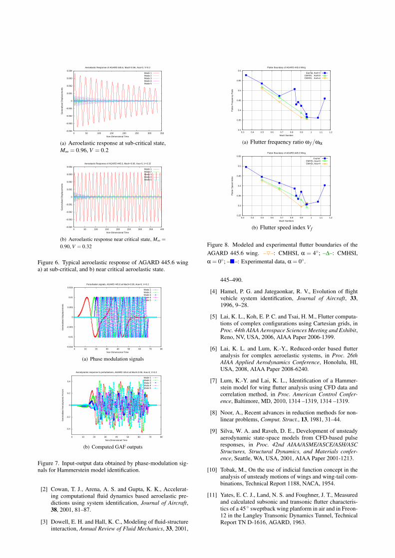
where A is the amplitude, ωc the central frequency, ωs the sweepferquency, and ∆ω the frequency semi-band. The parameters ofthis phase modulation signal are chosen in such a way that thesignal covers adequately the required range for the five naturalfrequencies of the wing. The prescribed generalised displace-ment and computed generalized aerodynamic forces (GAFs) fora typical case are shown in figure 7. Following the CHMSImethod and stability analysis, we obtained the critical speed in-dices and critical frequencies for the Mach numbers considered.The computed flutter boundaries is compared with experimen-tal results[11] in figure 8. The computational results are in goodagreement with experimental results across the Mach numberrange considered.

The CMHSI method was also exercised to investigate the flutterbehavior of the AGARD 445.6 wing at angle of attack α = 4.The solution, shown in figure 7, shows that the critical speedindex is reduced slightly as the attack angle is increased fromα = 0 to 4. This is probably due to an increase in aerody-namic forces as attack angle increases that triggers aeroelasticinstability to occur at a lower speed index.

Conclusions

A modeling and simulation framework for flutter analysis hasbeen developed using a combination of full-order computationalaeroelasticity techniques and reduced-order modeling methods.Flutter analyses were performed for the AGARD 445.6 wing aspart of the validation process. Results showed that the ROM-based predictions matched the experimental data well. Thecomputed flutter speed indices and flutter frequencies showedvery satisfactory results.

Acknowledgements

The authors would like to acknowledge support from the FSTDvia program agreement 9010102931.

References

[1] Ballhaus, W. F. and Goorjian, P. M., Computation of un-steady transonic flows by the indicial method, AIAA Jour-nal, 16, 1978, 117–124.

-0.004

-0.003

-0.002

-0.001

0

0.001

0.002

0.003

0.004

0 50 100 150 200 250 300 350

Gen

eral

ised

Dis

plac

emen

ts

Non-Dimensional Time

Aeroelastic Response of AGARD 445.6, Mach=0.96, Aoa=0, V=0.2

Mode 1Mode 2Mode 3Mode 4Mode 5

(a) Aeroelastic response at sub-critical state,M∞ = 0.96, V = 0.2

-0.004

-0.003

-0.002

-0.001

0

0.001

0.002

0.003

0.004

0 50 100 150 200 250 300 350 400

Gen

eral

ised

Dis

plac

emen

ts

Non-Dimensional Time

Aeroelastic Response of AGARD 445.6, Mach=0.90, Aoa=0, V=0.32

Mode 1Mode 2Mode 3Mode 4Mode 5

(b) Aeroelastic response near critical state, M∞ =0.90, V = 0.32

Figure 6. Typical aeroelastic response of AGARD 445.6 winga) at sub-critical, and b) near critical aeroelastic state.

-0.015

-0.01

-0.005

0

0.005

0.01

0.015

0 10 20 30 40 50 60 70 80

Gen

eral

ised

Dis

plac

emen

ts

Non-Dimensional Time

Perturbation signals, AGARD 445.6 at Mach=0.96, Aoa=0, V=0.2

Mode 1Mode 2Mode 3Mode 4Mode 5

(a) Phase modulation signals

-0.4

-0.2

0

0.2

0.4

0 10 20 30 40 50 60 70 80

Gen

eral

ised

Aer

odyn

amic

For

ces

Non-Dimensional Time

Aerodynamic response to perturbations, AGARD 445.6 at Mach=0.96, Aoa=0, V=0.2

Mode 1Mode 2Mode 3Mode 4Mode 5

(b) Computed GAF outputs

Figure 7. Input-output data obtained by phase-modulation sig-nals for Hammerstein model identification.

[2] Cowan, T. J., Arena, A. S. and Gupta, K. K., Accelerat-ing computational fluid dynamics based aeroelastic pre-dictions using system identification, Journal of Aircraft,38, 2001, 81–87.

[3] Dowell, E. H. and Hall, K. C., Modeling of fluid-structureinteraction, Annual Review of Fluid Mechanics, 33, 2001,

0.3

0.35

0.4

0.45

0.5

0.55

0.6

0.3 0.4 0.5 0.6 0.7 0.8 0.9 1 1.1 1.2

Flu

tter

Fre

quen

cy R

atio

Mach Number

Flutter Boundary of AGARD 445.6 Wing

Exp’tal, AoA=0CMHSI, AoA=0CMHSI, AoA=4

(a) Flutter frequency ratio ω f /ωα

0.25

0.3

0.35

0.4

0.45

0.5

0.55

0.3 0.4 0.5 0.6 0.7 0.8 0.9 1 1.1 1.2

Flu

tter

Spe

ed In

dex

Mach Numbers

Flutter Boundary of AGARD 445.6 Wing

Exp’tal CMHSI, Aoa=0CMHSI, Aoa=4

(b) Flutter speed index V f

Figure 8. Modeled and experimental flutter boundaries of theAGARD 445.6 wing. –O–: CMHSI, α = 4; –∆–: CMHSI,α = 0; ––: Experimental data, α = 0.

445–490.

[4] Hamel, P. G. and Jategaonkar, R. V., Evolution of flightvehicle system identification, Journal of Aircraft, 33,1996, 9–28.

[5] Lai, K. L., Koh, E. P. C. and Tsai, H. M., Flutter computa-tions of complex configurations using Cartesian grids, inProc. 44th AIAA Aerospace Sciences Meeting and Exhibit,Reno, NV, USA, 2006, AIAA Paper 2006-1399.

[6] Lai, K. L. and Lum, K.-Y., Reduced-order based flutteranalysis for complex aeroelastic systems, in Proc. 26thAIAA Applied Aerodynamics Conference, Honolulu, HI,USA, 2008, AIAA Paper 2008-6240.

[7] Lum, K.-Y. and Lai, K. L., Identification of a Hammer-stein model for wing flutter analysis using CFD data andcorrelation method, in Proc. American Control Confer-ence, Baltimore, MD, 2010, 1314 –1319, 1314 –1319.

[8] Noor, A., Recent advances in reduction methods for non-linear problems, Comput. Struct., 13, 1981, 31–44.

[9] Silva, W. A. and Raveh, D. E., Development of unsteadyaerodynamic state-space models from CFD-based pulseresponses, in Proc. 42nd AIAA/ASME/ASCE/ASH/ASCStructures, Structural Dynamics, and Materials confer-ence, Seattle, WA, USA, 2001, AIAA Paper 2001-1213.

[10] Tobak, M., On the use of indicial function concept in theanalysis of unsteady motions of wings and wing-tail com-binations, Technical Report 1188, NACA, 1954.

[11] Yates, E. C. J., Land, N. S. and Foughner, J. T., Measuredand calculated subsonic and transonic flutter characteris-tics of a 45 sweptback wing planform in air and in Freon-12 in the Langley Transonic Dynamics Tunnel, TechnicalReport TN D-1616, AGARD, 1963.