journal of fluid mechanics laminar and turbulent...

Journal of Fluid Mechanicshttp://journals.cambridge.org/FLM

Additional services for Journal of Fluid Mechanics:

Email alerts: Click hereSubscriptions: Click hereCommercial reprints: Click hereTerms of use : Click here

Laminar and turbulent comparisons for channel flow and flow control

IVAN MARUSIC, D. D. JOSEPH and KRISHNAN MAHESH

Journal of Fluid Mechanics / Volume 570 / January 2007, pp 467 477DOI: 10.1017/S0022112006003247, Published online: 03 January 2007

Link to this article: http://journals.cambridge.org/abstract_S0022112006003247

How to cite this article:IVAN MARUSIC, D. D. JOSEPH and KRISHNAN MAHESH (2007). Laminar and turbulent comparisons for channel flow and flow control. Journal of Fluid Mechanics, 570, pp 467477 doi:10.1017/S0022112006003247

Request Permissions : Click here

Downloaded from http://journals.cambridge.org/FLM, IP address: 128.250.144.147 on 23 Oct 2012

J. Fluid Mech. (2007), vol. 570, pp. 467–477. c© 2007 Cambridge University Press

doi:10.1017/S0022112006003247 Printed in the United Kingdom

467

Laminar and turbulent comparisons forchannel flow and flow control

By IVAN MARUSIC, D. D. JOSEPHAND KRISHNAN MAHESH

Department of Aerospace Engineering and Mechanics, University of Minnesota,Minneapolis, MN 55455, USA

(Received 3 May 2006 and in revised form 14 August 2006)

A formula is derived that shows exactly how much the discrepancy between thevolume flux in laminar and in turbulent flow at the same pressure gradient increasesas the pressure gradient is increased. We compare laminar and turbulent flows inchannels with and without flow control. For the related problem of a fixed bulk-Reynolds-number flow, we seek the theoretical lowest bound for skin-friction dragfor control schemes that use surface blowing and suction with zero-net volume-fluxaddition. For one such case, using a crossflow approach, we show that sustaineddrag below that of the laminar-Poiseuille-flow case is not possible. For more generalcontrol strategies we derive a criterion for achieving sublaminar drag and use thisto consider the implications for control strategy design and the limitations at highReynolds numbers.

1. IntroductionIt is well known that in channels and pipes the volume flux of laminar flow is

greater than that for turbulent flow at the same pressure gradient (Thomas 1942).Equivalently, the skin-friction drag in a laminar flow is less than in a turbulent flowfor the same volume flux. In this paper we derive a formula to compute this volume-flux discrepancy for a given pressure gradient and consider the implications at highReynolds numbers.

It has been conjectured (e.g. Bewley 2000) that, for constant volume-flux flows,sustained sublaminar drag is not possible even in the presence of flow control. Bewleyconsidered zero-net volume-flux blowing or suction at the no-slip walls as a controlstrategy. (For the case of a fixed pressure gradient, the equivalent conjecture would bethat such flow control cannot produce an average volume flux in excess of the laminarvalue.) However, several studies including Bewley & Aamo (2004) and Cortelezzi et al.(1998), have demonstrated transient drag reductions below the laminar level. Recently,Min, Kang, Speyer & Kim (2006) demonstrated that sustained sublaminar drag can infact be achieved in a fully developed channel flow, albeit at a low Reynolds number.By ‘sustained drag’ we mean that the average value of the drag is independent oftime. Min et al. (2006) used direct numerical simulations in an open-loop controlstrategy, with wall blowing and suction in the form of an upstream travelling wave,to achieve their result.

In this paper we consider laminar- and turbulent-flow comparisons forincompressible channel flows, with and without control, and discuss the implicationsfor a range of Reynolds numbers. Two types of zero net-volume-flux blowing and

468 I. Marusic, D. D. Joseph and K. Mahesh

suction control strategies are investigated. The first involves uniform-control flowacross the channel, as was used by Fukagata, Iwamoto & Kasagi (2002), and forthis case we prove that sustained drag below that of the laminar-Poiseuille-flow caseis not possible. The second control strategy addresses the more general case, withzero-mean flow at the walls, as was considered by Bewley & Aamo (2004) and others.For this case we obtain a criterion for sustained sub-laminar conditions based on thepower input of the control flow. Consideration of the criterion sheds light on whythe control scheme of Min et al. (2006) was successful and indicates directions formodified control strategies that might yield further improvements.

2. Equations for channel flowMuch of the following extends the analyses presented by Busse (1970), Howard

(1972) and Joseph (1974), who considered channel flows without control.For a fully developed channel flow of an incompressible fluid, driven by a constant

pressure gradient, the Navier–Stokes and continuity equations may be written as

∂V∂t

+ V · ∇V = −∇p + exP + ∇2V , (2.1)

∇ · V = 0. (2.2)

The Cartesian coordinate system used here defines x and y as the streamwise andspanwise directions respectively, and z is the distance in the wall-normal directionfrom the centre of the channel. Unless indicated, here all terms have been non-dimensionalized using ν, the kinematic viscosity of the fluid, and d , the height of thechannel. The domain occupied by the fluid is

−∞ < x, y < ∞; −1/2 � z � 1/2.

Here P > 0 is the constant pressure gradient driving the flow, and the total pressureat a point in the fluid is

p(x, y, z, t) − Px,

where in all cases pressure has been normalized by ρ, the fluid density. We denote awall-parallel plane average with an overbar:

f (z, t) = limL→∞

1

(2L)2

∫ L

−L

∫ L

−L

f (x, y, z, t) dx dy,

and the overall average as

〈f 〉 =

∫ 1/2

−1/2

f dz.

Therefore, the Reynolds number ReB = 〈Vx〉 is that based on the channel heightand the bulk velocity. We will also decompose the velocity and pressure into mean(wall-parallel plane-averaged) and fluctuating parts,

V = V + u, p = p + p′, (2.3)

where the fluctuations have a zero mean: u, v, w, p′ = 0.

2.1. Boundary conditions

We consider three types of channel flow. For all three cases

Vx = Vy = 0 at z = ±1/2

Laminar and turbulent comparisons 469

while we have

for case 1, Vz = 0 at z = ±1/2;for case 2, Vz = C(t) at z = ±1/2, where C = constant;for case 3, Vz = φ+(x, y, t) at z = 1/2 and φ−(x, y, t) at z = −1/2, where φ+ =

φ− = 0.

Note that u = v = 0 at z ± 1/2 for all three cases, but w = φ = 0 for cases 1 and2 only. Case 1 is conventional channel flow, while cases 2 and 3 cover the possibleflows with blowing or suction at the walls and with zero net-volume-flux addition.For case 2, any flow introduced through the bottom wall is balanced by flow leavingthe top wall. This flow was considered in control studies by Fukagata et al. (2002).Case 3 is the case considered by Bewley & Aamo (2004), Min et al. (2006) and others;it allows for different functions for Vz on the top and bottom walls provided thattheir mean is zero.

2.2. Energy equations

In the following we will make use of energy identities. These are derived first bysubstituting (2.3) into (2.1) and using continuity to give

∂ V∂t

+∂u∂t

+ Vz

∂ V∂z

+ ∇ · (V u + uV + uu) = − ez∂p

∂z− ∇p′ + exP +

∂2V∂z2

+ ∇2u. (2.4)

For cases 1 and 3, Vz = 0 everywhere owing to (2.2), while for case 2, Vz = C. Thewall-parallel plane average of (2.4) is

∂ V∂t

+ Vz

∂ V∂z

+ ∇ · (uu) = −ez∂p

∂z+ exP +

∂2V∂z2

, (2.5)

and the difference (2.4)–(2.5) is

∂u∂t

+ ∇ · (V u + uV + uu − uu) = −∇p′ + ∇2u. (2.6)

An energy identity for the mean component is found by forming the dot product ofV with (2.5), taking the average and setting the result to zero, i.e. 〈V · (2.5)〉 = 0,which gives

1

2

d

dt〈|V |2〉 +

⟨Vx

∂uw

∂z+ Vy

∂vw

∂z

⟩= P 〈Vx〉 + Vz[p]∓ −

⟨∣∣∣∣∂Vx

∂z

∣∣∣∣2

+

∣∣∣∣∂Vy

∂z

∣∣∣∣2⟩

, (2.7)

where the notation [ ]∓ indicates that the quantity at z = 1/2 is subtracted from thequantity at z = −1/2, i.e. [p]∓ = p− − p+. The corresponding energy identity for thefluctuating parts is found from forming 〈u · (2.6)〉 = 0, which gives

1

2

d

dt〈|u|2〉 +

⟨uw

∂Vx

∂z+ vw

∂Vy

∂z

⟩= Γ − 〈|∇u|2〉, (2.8)

where

Γ = [φ(p′ + φ2/2)]∓. (2.9)

(Here we note that u · ∂u/∂z = 0 at the walls for all three cases. This can be shown byusing Taylor series expansions, the continuity equation and the boundary conditions.)

Summing (2.7) and (2.8) gives the total energy equation

1

2

d

dt〈|V |2 + |u|2〉 = P 〈Vx〉 + Vz[p]∓ + Γ −

⟨|∇u|2 +

∣∣∣∣∂Vx

∂z

∣∣∣∣2

+

∣∣∣∣∂Vy

∂z

∣∣∣∣2⟩

. (2.10)


It may be noted that in addition to the driving pressure-gradient work term, P 〈Vx〉,an extra energy-source term exists for case 2 owing to another pressure-gradient workterm, Vz[p]∓, while for case 3 the extra term is Γ , which is due to the control flow atthe walls and the associated induced fluctuating pressures.

3. Volume-flux comparison between laminar and turbulent flowsFirst we consider laminar Poiseuille flow (case 1 with u = 0). Here V = (Ul(z), 0, 0)

and (2.1) has the solution

Ul(z) = 32〈Ul〉(1 − 4z2) (3.1)

for

Pl = −d2Ul

dz2= 12〈Ul〉. (3.2)

In order to evaluate the bulk flow rate for the turbulent-flow case, 〈Vx〉, wespecify two properties of statistical stationarity. The first is that all wall-parallel planeaverages, indicated by overbars, are time independent, and second we assume thatvelocity components have a zero mean value unless a non-zero mean value is forcedexternally. This latter property implies Vy = 0 for all flows considered here. Undersuch conditions (2.5) may be written as

d

dz

[exVxVz + uw + ezp − exPz − dV

dz

]= 0, (3.3)

where VxVz = VxVz, since Vz = 0 or a constant. The energy equation (2.8) becomes

−⟨

uwdVx

dz

⟩+ Γ = 〈|∇u|2〉. (3.4)

We now seek an expression for P by taking the first integral of the x-component of(3.3):

Pz = uw + VxVz − 〈uw〉 − 〈VxVz〉 − dVx

dz. (3.5)

The above equation is similar to the well-known linear relation for the stress. Forming〈z · (3.5)〉 = 0 gives

P = 12〈z(uw + VxVz)〉 + 12〈Vx〉. (3.6)

The above equation is identical to that given by Fukugata et al. (2002) (equation(16) in their paper). A comparison between the volume flux in the channel for aturbulent flow with control and for the base laminar flow can now be made. For flowswith the same driving pressure gradient (P = Pl), using (3.6) and (3.2) the differencein the bulk flow rates for fully developed laminar flows and for turbulent flows isgiven by

〈Ul − Vx〉 = 〈z(uw + VxVz)〉. (3.7)

Therefore a proof that zero net-volume-flux blowing or suction control cannot producea volume flux in excess of laminar flow requires

〈z(uw + VxVz)〉 � 0. (3.8)

To test this we form 〈(uw + VxVz) · (3.5)〉 = 0 and using (3.4) obtain after somemanipulation

P 〈z(uw + VxVz)〉 = 〈|∇u|2〉 + 〈[(uw + VxVz) − (〈uw〉 + 〈VxVz〉)]2〉 − Γ. (3.9)


Turbulent

Laminar

Reτ = 186

x

z

Figure 1. The turbulent mean-velocity profile, from the DNS dataset of del Alamo & Jimenez(2003) at Reτ = 186, and the corresponding laminar profile for the same driving pressuregradient. The profiles are drawn to scale (relative to each other).

Here P > 0 by definition and, therefore, (3.9) indicates that (3.8) holds for case 2,since φ = 0 and hence Γ = 0 and all other terms on the right-hand side are positive.However, for case 3, where Vz = 0, the controlled flow can produce a volume flux inexcess of laminar flow if and only if

Γ > 〈|∇u|2〉 + 〈[uw − 〈uw〉]2〉. (3.10)

The same criterion holds for producing sublaminar drag, as will be discussed in § 4.Although the drag is sublaminar, the power required to drive the flow may not beless than the laminar value (e.g. Choi, Moin & Kim 1994, p. 79). Also, we note thatthe right-hand side of (3.10) will change with φ, and the expression itself does notsuggest a practical design strategy. However, it is clear that any control that yieldssublaminar drag needs to satisfy (3.10) and that the specific term [φ(p′ + φ2/2)]∓needs to be positive. This will be further discussed in § 4.1.

3.1. Quantitative comparisons

For regular channel flows and flows with crossflow control strategies (cases 1 and 2in § 2.1), the right-hand side of (3.7) is, as shown above, always positive, and hencethe bulk flow rate for the laminar case is always higher for these flows. This is a moregeneral statement of the ‘mass-flux-discrepancy theorem’ of Busse (1970) and Joseph(1974). A formal proof of this for regular pipe flow was first given by Thomas (1942).For regular channel flow, the result is well illustrated in figure 1, where a turbulentmean-velocity profile, taken from a direct numerical simulation (DNS) dataset atReτ = 186, together with, for comparison, the corresponding laminar profile (3.1) forthe same level of driving pressure gradient. (Here Reτ is the Karman number, which isdefined as the Reynolds number based on the channel half-width and the skin-frictionvelocity Uτ = (τ0/ρ)1/2.) The condition P = Pl requires that the wall-normal gradientsof the velocity profiles be equal at the walls.

While it is well known that the flow rate is higher in laminar than in turbulentflow at the same pressure gradient, we are not aware of any formula other thanthe one derived here from which the flow rates may be calculated. For example, theabove results indicate that a laminar channel or pipe flow in transition to turbulencewill always be associated with a bulk deceleration of the flow. Given the confinedgeometry, this transient event can only manifest itself through an adverse pressuregradient (i.e. one that is opposite to the driving pressure gradient). Few articles inthe literature have reported this, an exception being a recent study by van Doorne(2004). Quantitative differences between the bulk flow rates (or volume fluxes) can be


102 103 104 105

Reτ

100

101

102

103

�Vx�

�Ul�

Figure 2. The ratio of the bulk velocities for laminar and turbulent channel flows as afunction of Reτ . The solid line corresponds to (3.13). The dashed line corresponds to the sameresult but with the skin-friction formulae of Dean (1978). The solid circles are from the DNSdatasets of del Alamo & Jimenez (2003), del Alamo et al. (2004) and Hoyas & Jimenez (2006).The Reτ = 186 ordinate corresponds to the profiles in figure 1. The dotted line correspondsto the expression for pipe flow. The dotted circles are from the pipe experiments of McKeonet al. (2004).

obtained using functional forms for the mean-velocity profiles (laminar and turbulent).For instance, using a law-of-the-wall-wake mean-velocity formulation, such as thatgiven by Perry, Marusic & Jones (2002) (their equation (4.6)) it can be shown that

〈Vx〉 − V1

Uτ

≈ − 1

κ, (3.11)

where V1 and Uτ are the non-dimensional centre-line and skin-friction velocitiesrespectively and

V1

Uτ

=1

κln Reτ + A +

1

κ

(2Π − 1

3

); (3.12)

here we take κ = 0.41, A = 5.0 and the Coles wake factor Π = 0.2. From (3.2) wecan show that the laminar bulk velocity 〈Ul〉 = 2Re2

τ /3, and using (3.7) for regularchannel flows, with (3.11) and (3.12), we obtain

〈Ul − Vx〉 = 〈zuw〉 = 23Re2

τ − 2

κReτ (ln Reτ + C), (3.13)

where P = 8Re2τ and C = κA + 2Π − 4/3 = 1.117, using the values given above.

Figure 2 shows for comparison the bulk velocities for laminar and turbulent flowsfor varying levels of Reτ . The solid line is obtained using the above expressions forchannel flows. For a typical practical Reynolds number Reτ = 105 the ratio 〈Ul〉/〈Vx〉is seen to be over 1000.† The ratio of the laminar and turbulent velocities is alsoa convenient way of illustrating how 〈zuw〉 changes with Reτ , and a correspondingplot is shown in figure 3; the asymptotic trend is equivalent to the condition that the

† This example is in the spirit of A. N. Kolmogorov who, as explained by Barenblatt (2005),would start his course on turbulence at Moscow State University by asking the students what theflow rate of the Volga river would be if by some miracle it became laminar. The answer is striking,with surface velocities in the hundreds of kilometres per second.


102 103 104 105

Reτ

0.45

0.50

0.55

0.60

0.65

0.70

�zuw�

Re2τ

2/3

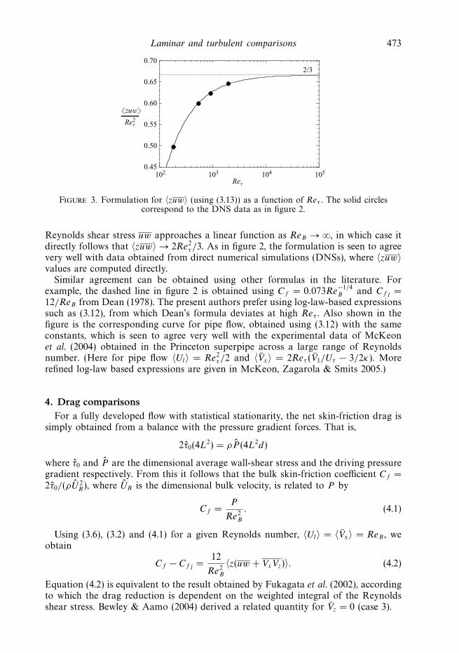
Figure 3. Formulation for 〈zuw〉 (using (3.13)) as a function of Reτ . The solid circlescorrespond to the DNS data as in figure 2.

Reynolds shear stress uw approaches a linear function as ReB → ∞, in which case itdirectly follows that 〈zuw〉 → 2Re2

τ /3. As in figure 2, the formulation is seen to agreevery well with data obtained from direct numerical simulations (DNSs), where 〈zuw〉values are computed directly.

Similar agreement can be obtained using other formulas in the literature. Forexample, the dashed line in figure 2 is obtained using Cf = 0.073Re−1/4

B and Cf l=

12/ReB from Dean (1978). The present authors prefer using log-law-based expressionssuch as (3.12), from which Dean’s formula deviates at high Reτ . Also shown in thefigure is the corresponding curve for pipe flow, obtained using (3.12) with the sameconstants, which is seen to agree very well with the experimental data of McKeonet al. (2004) obtained in the Princeton superpipe across a large range of Reynoldsnumber. (Here for pipe flow 〈Ul〉 = Re2

τ /2 and 〈Vx〉 = 2Reτ (V1/Uτ − 3/2κ). Morerefined log-law based expressions are given in McKeon, Zagarola & Smits 2005.)

4. Drag comparisonsFor a fully developed flow with statistical stationarity, the net skin-friction drag is

simply obtained from a balance with the pressure gradient forces. That is,

2τ0(4L2) = ρP (4L2d)

where τ0 and P are the dimensional average wall-shear stress and the driving pressuregradient respectively. From this it follows that the bulk skin-friction coefficient Cf =2τ0/(ρU 2

B), where UB is the dimensional bulk velocity, is related to P by

Cf =P

Re2B

. (4.1)

Using (3.6), (3.2) and (4.1) for a given Reynolds number, 〈Ul〉 = 〈Vx〉 = ReB , weobtain

Cf − Cf l=

12

Re2B

〈z(uw + VxVz)〉. (4.2)

Equation (4.2) is equivalent to the result obtained by Fukagata et al. (2002), accordingto which the drag reduction is dependent on the weighted integral of the Reynoldsshear stress. Bewley & Aamo (2004) derived a related quantity for Vz = 0 (case 3).


As expected, the criterion for achieving sublaminar drag with control for a fixedvolume flux is equivalent to exceeding the volume flux of laminar flow for a fixedpressure gradient. Both depend on 〈z(uw + VxVz)〉. Therefore, from (3.7) and (3.9) wemay also conclude that for regular channel flows and flows with crossflow controlstrategies (cases 1 and 2)

Cf − Cf l� 0. (4.3)

For case 3, where Vz = 0, (3.10) holds and therefore the controlled flow can producesustained sublaminar skin-friction levels if and only if

Γ > 〈|∇u|2〉 + 〈[uw − 〈uw〉]2〉.

4.1. Implications for control strategies

Equation (3.10) gives the criterion for achieving sustained sublaminar drag; from itwe may identify the relevant control parameter Γ = [φ(p′ + φ2/2)]∓, which is solelydefined on the walls of the channel. The criterion does not directly yield a practicaldesign strategy but does provide insights into strategies that have been proposed inthe literature.

In (3.10), Γ relates to the power input of the control signal, and as expectedincreasing Γ decreases the net skin-friction drag. However, it may be noted thatmaximizing Γ requires a control strategy that sums the contributions from theopposing walls. Therefore, in order to consider a physical interpretation for Γ werestrict our attention to the bottom wall in flows with symmetric actuation. In thiscase we require that [φ(p′ + φ2/2)]− be positive. For any periodic blowing and suction(as was used by Min et al. 2006) φ3 yields zero when averaged, and therefore the onlycontribution to Γ can come from p′φ. We therefore require that blowing (positive φ)be accompanied by an increase in pressure, while suction (negative φ) be accompaniedby a decrease in pressure at the wall.

It is known from studies on jets in crossflow (e.g. Muppidi & Mahesh 2005) that acrossflowing jet yields high levels of pressure, especially at the leading edge of the jet;i.e. a positive value of φ yields positive values of p′. Similarly, high levels of suctionwill modify the local flow to resemble a point sink. The external flow acceleratestoward the source of suction, in order to conserve mass; the acceleration sets up afavourable pressure gradient in the direction of the suction and therefore decreasesthe pressure at the source of suction. Negative values of φ therefore produce negativevalues of p′ and so the resulting product is positive.

To test this interpretation, direct numerical simulations were carried out foridealized flows with blowing and suction into a cross-stream, using the numericalapproach as described by Muppidi & Mahesh (2005). The geometry is that of a two-dimensional channel with dimensions 20×10×1 per unit slot width, in the streamwise,wall-normal and spanwise directions respectively. The width of the slot extends overthe entire span, over which periodic conditions are imposed. Free-stream Dirichletconditions are prescribed at the top boundary, and convective boundary conditionsare prescribed at the outflow. Note that the domain height is large enough not toaffect the solution. A top-hat profile is prescribed for the jet through the slot, anda uniform crossflow is prescribed at the inflow. Along the bottom wall, the uniformcrossflow forms a boundary layer whose thickness with respect to the jet is small.The simulation results therefore depend essentially upon the parameter rs, where r

denotes the velocity ratio of the jet and the crossflow and s denotes the slot width.While these flows are simplified, the general trends are expected to hold very near

the blowing and suction ports since Γ is a quantity evaluated exactly at the wall.


–2 –1 30 1 2 –2 –1 30 1 2 x/s

–0.2

0

0.2

0.4 p'φ

–1.0

–0.5

0.0

0.5

–0.2

0

0.2

0.4

–1.0

–0.5

0.0

0.5φ

p'

Suction

x/s

p'φ

φ

p'

Blowing

Figure 4. Numerical-simulation results for two-dimensional blowing and suction into acrossflow, moving from right to left. The blowing and suction flows are initially applieduniformly across 0 � x/s � 1. The wall velocities and pressures here are normalized by thecrossflow velocity. Note that the average value of p′φ on the wall for both blowing and suctionis positive.

The results are shown in figure 4 where, for both blowing and suction, p′φ is foundto be positive provided that the level of blowing and suction is sufficiently high. Forinstance, in figure 4 the ratio of φ and the crossflow speed was 0.5, while a ratio of0.1 was found to be insufficient to produce a positive p′φ value.

The above mechanism for generating high p′φ values on the bottom wall isconsistent with the approach used by Min et al. (2006), who demonstrated sublaminardrag using a travelling wave blowing and suction strategy with

φ = a cos[α(x − ct)], (4.4)

where c is the wave speed. Relatively high levels of blowing and suction were requiredby Min et al. (2006) to achieve sublaminar drag combined with upstream travellingwaves (c negative). The control flow was also implemented on both walls in varicosemode, i.e. the upper and lower walls have blowing and suction in phase at the samestreamwise location. This symmetric actuation is consistent with adding the effectsfrom the top and bottom walls while an upward-travelling wave increases the relativevelocity between the jet and the crossflow, which means that for the same jet velocityφ, the stagnation pressure p′ at the leading edge of the jet would be higher; i.e.the upward-traveling wave generates higher positive levels of p′φ. Conversely, adownward-traveling wave would, for small phase speeds, decrease the relative velocityand thereby decrease the stagnation pressure at the jet leading edge. The resultingvalue of p′φ would be smaller and therefore less effective in reducing drag. If thedownstream wave speed is large enough, then the crossflow would have to acceleratein the streamwise direction to occupy the region evacuated by the jet; the accelerationwould decrease the pressure in the vicinity of the jet, i.e. p′φ would be negative, and


the drag would actually increase. This is consistent with what Min et al. (2006) foundfor positive values of c.

Considering (3.10) and the expression for Γ it would seem that the control strategyused by Min et al. (2006) could perhaps be further improved by modifying the controlto yield positive and negative values of φ3 on the bottom and top walls respectively.This would require that the input control flow be skewed. Since from the results infigure 4 it appears that suction has a higher contribution to p′φ than does blowing,this would indicate that possibly using a symmetric varicose blowing and suctionupstream-travelling waveform that is biased towards more intense suction (while stillmaintaining φ = 0) might be beneficial.

5. Concluding remarksFor turbulence control, it is necessary to understand how to achieve sublaminar

levels of drag at high Reynolds numbers. For the general blowing and suction controlstrategy (case 3) this relates directly to 〈zuw〉. Figure 3 shows that 〈zuw〉 has veryhigh values at high Reynolds numbers (since it increases nominally with Re2

τ ), whichmakes relaminarization or sublaminar drag reduction by control difficult. Min et al.(2006) achieved sublaminar conditions at Reτ ≈ 120, but at high Reynolds numbersfigure 2 shows that 〈zuw〉 would be many orders of magnitude higher. However, acontrol scheme need not relaminarize a flow from a high Reynolds number but couldinstead modify the Reynolds shear-stress profile in such a way as to minimize theweighted integral 〈zuw〉. Iwamoto et al. (2005) used this strategy recently and showedthat small changes to uw in the near-wall region at high Reynolds number can leadto substantial reductions in skin friction.

Comparison of the volume flux for laminar and turbulent flows for a given pressuregradient also highlights that, in general, reducing the turbulence level in flows drivenby a steady energy source can lead to significant increases of mean velocity. Anotherexample of this, which in the authors’ opinion is worth mentioning, relates to themodification of turbulence by the transport of small particles (Gore & Crowe 1989).Barenblatt, Chorin & Prostokishin (2005) considered such a mechanism to explainwhy accelerated levels of wind speed exist in tropical cyclones in regions near the watersurface, where ocean spray droplets reside. Here it is believed that the turbulenceenergy that goes into suspending the particles in the flow leads to a reduction inthe flow turbulence intensity and consequently dramatic increases in the mean windspeed. Similar mechanisms may explain why sand storms are typically associated withhigh sustained wind speeds, which allow the storm to travel over very long distances.

This work was in part supported by the National Science Foundation (IM withCTS-0324898, DDJ with CTS-0302837 and KM with CTS-0133837), and the Davidand Lucile Packard Foundation. We are also grateful to Suman Muppidi for usefuldiscussions.

REFERENCES

del Alamo, J. C. & Jimenez, J. 2003 Spectra of the very large anisotropic scales in turbulentchannels. Phys. Fluids 15 (6), L41–L44.

del Alamo, J. C., Jimenez, J., Zandonade, P. & Moser, R. D. 2004 Scaling of the energy spectraof turbulent channels. J. Fluid Mech. 500, 135–144.

Barenblatt, G. I. 2005 Applied mechanics: an age old science perpetually in rebirth. ASMETimoshenko Medal Acceptance Speech .


Barenblatt, G. I., Chorin, A. J. & Prostokishin, V. M. 2005 A note concerning the Lighthill‘sandwich model’ of tropical cyclones. Proc. Natl Acad. Sci. 102, 11148–11150.

Bewley, T. R. 2001 Flow control: new challenges for a new renaissance. Prog. Aerospace Sci. 37,21.

Bewley, T. R. & Aamo, O. M. 2004 A ‘win-win’ mechanism for low-drag transients in controlledtwo-dimensional channel flow and its implications for sustained drag reduction. J. Fluid Mech.499, 183–196.

Busse, F. H. 1970 Bounds for turbulent shear flow. J. Fluid Mech. 41, 219–240.

Choi, H., Moin, P. & Kim, J. 1994 Active turbulence control for drag reduction in wall-boundedflows. J. Fluid Mech. 262, 75–110.

Cortelezzi, L., Lee, K. H., Kim, J. & Speyer, J. L. 1998 Skin-friction drag reduction via robustreduced-order linear feedback control. Intl J. Comput. Fluid Dyn. 11, 79–92.

Dean, R. B. 1978 Reynolds number dependence of skin friction and other bulk flow variables intwo-dimensional rectangular duct flow. Trans. ASME: J. Fluids Engng 100, 215–223.

van Doorne, C. W. H. 2004 Stereoscopic PIV on transition in pipe flow. PhD thesis, TU-Delft,Netherlands.

Fukagata, K., Iwamoto, K. & Kasagi, N. 2002 Contribution of Reynolds stress distribution to theskin friction in wall-bounded flows. Phys. Fluids 14 (11), L73–L76.

Gore, R. & Crowe, C. 1989 Effect of particle size on modulating turbulent intensity. Intl J.Multiphase Flow 15, 279–285.

Howard, L. N. 1972 Bounds on flow quantities. Annu. Rev. Fluid Mech. 4, 473–494.

Hoyas, S. & Jimenez, J. 2006 Scaling of the velocity fluctuations in turbulent channels up toReτ = 2003. Phys. Fluids 18, 011702.

Iwamoto, K., Fukagata, K., Kasagi, N. & Suzuki, Y. 2005 Friction drag reduction achievable bynear-wall turbulence manipulation at high Reynolds number. Phys. Fluids 17, 011702.

Joseph, D. D. 1974 Response curves for plane Poiseuille flow. Adv. Appli. Mech. 14, 241–278.

McKeon, B., Li, J., Jiang, W., Morrison, J. & Smits, A. 2004 Further observations on the meanvelocity in fully-developed pipe flow. J. Fluid Mech. 501, 135–147.

McKeon, B., Zagarola, M. & Smits, A. 2005 A new friction factor relationship for fully developedpipe flow. J. Fluid Mech. 538, 429–443.

Min, T., Kang, S., Speyer, J. L. & Kim, J. 2006 Sustained sub-laminar drag in a fully developedchannel flow. J. Fluid Mech. 558, 309–318.

Muppidi, S. & Mahesh, K. 2005 Study of trajectories of jets in crossflow using direct numericalsimulations. J. Fluid Mech. 530, 81–100.

Perry, A. E., Marusic, I. & Jones, M. B. 2002 On the streamwise evolution of turbulent boundarylayers in arbitrary pressure gradients. J. Fluid Mech. 461, 61–91.

Thomas, T. Y. 1942 Qualitative analysis of the flow of fluids in pipes. Am. J. Maths 64, 754–767.

journal of fluid mechanics laminar and turbulent...

Documents