heavy-duty engines conformity testing based on pems

EUR 24921 EN - 2011

HEAVY-DUTY ENGINES CONFORMITY TESTING BASED

ON PEMSLessons Learned from the European Pilot Program

Pierre Bonnel - Janek Kubelt - Alessio Provenza

The mission of the JRC-IE is to provide scientific-technical support to the European Union’s policies for the protection and sustainable development of the European and global environment. European Commission Joint Research Centre Institute for Energy Contact information Authors for correspondence: Pierre Bonnel, Alessio Provenza Sustainable Transport Unit, TP 441, 21020 Ispra (VA), Italy Email: [email protected] http://ie.jrc.ec.europa.eu/ http://www.jrc.ec.europa.eu/ Legal Notice Neither the European Commission nor any person acting on behalf of the Commission is responsible for the use which might be made of this publication.

Europe Direct is a service to help you find answers to your questions about the European Union

Freephone number (*):

00 800 6 7 8 9 10 11

(*) Certain mobile telephone operators do not allow access to 00 800 numbers or these calls may be billed.

A great deal of additional information on the European Union is available on the Internet. It can be accessed through the Europa server http://europa.eu/ JRC 66031 EUR 24921 EN ISBN 978-92-79-21038-9 (print), ISBN 978-92-79-21039-6 (online) ISSN 1018-5593 (print), ISSN 1831-9424 (online) doi:10.2788/56535 Luxembourg: Publications Office of the European Union © European Union, 2011 Reproduction is authorised provided the source is acknowledged Printed in Luxembourg

In collaboration with: MM. Jan Kruithof, Jeroen Smits (DAF TRUCKS) Mr. Juergen Stein (DAIMLER CHRYSLER) MM. Arthur Stark, Meinrad Signer (IVECO) MM. Robert Rothenaicher (MAN) MM.Guenter Kleinschek, Sven Andersson (SCANIA) Mr. Alf Ekermo, Jonas Holmberg, Jean-Francois Renaudin (VOLVO POWERTRAIN) Mr Bjorn Ramacher (VW) Mr Lennart Erlandsson (AVL MTC) Mr Hakan Johansson (Swedish Road Administration) Mr. Henk Dekker (TNO) Mr Leif-Erik Schulte (TUEV NORD) MM. Petter ASMAN, Ferenc PEKAR (European Commission, DG ENTR)

Table of contents 1 List of acronyms ................................................................................... 5 2 Background and objectives ..................................................................... 6

2.1 Initial steps: the EU-PEMS project ..................................................... 6 2.2 EU heavy-duty pilot program ............................................................ 6 2.3 Objectives of the work ..................................................................... 7

3 EU-PEMS Pilot Program data set .............................................................. 8 3.1 Introduction .................................................................................... 8 3.2 Vehicles and engines ........................................................................ 8 3.3 Test equipment ............................................................................... 8 3.4 Test routes ..................................................................................... 9

3.4.1 Average route characteristics ....................................................... 9 3.4.2 Analysis of trip characteristics .................................................... 12

3.5 Data handling procedures and tools ................................................. 14 3.5.1 Test data ................................................................................ 14 3.5.2 Time alignment ........................................................................ 14 3.5.3 EMROAD© .............................................................................. 15 3.5.4 Data consistency checks ........................................................... 16 3.5.5 Plausibility of BSFC values ......................................................... 18

3.6 Average results ............................................................................. 19 4 In-Service Conformity Emissions Evaluation ........................................... 21

4.1 Introduction .................................................................................. 21 4.2 Control area methods ..................................................................... 21

4.2.1 Introduction ............................................................................ 21 4.2.2 Effect of control are methods on data sets................................... 22 4.2.3 Conclusions on the control area methods .................................... 23

4.3 Averaging window methods ............................................................ 24 4.3.1 Introduction ............................................................................ 24 4.3.2 Averaging window calculations ................................................... 24 4.3.3 Calculation of the specific emissions ........................................... 26 4.3.4 Calculation of the conformity factors ........................................... 26 4.3.5 Maximum allowed conformity factor ........................................... 27 4.3.6 Calculation steps ...................................................................... 27

4.4 Results with the averaging window method ....................................... 28 4.4.1 Introduction ............................................................................ 28 4.4.2 Overview of brake-specific results for all vehicles ......................... 28 4.4.3 NOx Conformity Factors for all vehicles ....................................... 30 4.4.4 Test to test variability ............................................................... 31 4.4.5 Case studies ............................................................................ 33

4.5 Settings of the averaging window method ......................................... 40 4.5.1 Power threshold ....................................................................... 40 4.5.2 Effect of idling ......................................................................... 41 4.5.3 Reference quantity: work or CO2 mass? ...................................... 43

4.6 Conclusions on the averaging window methods ................................. 46 5 Lessons learned .................................................................................. 49

5.1 Data quality .................................................................................. 49 5.2 Data evaluation methods ................................................................ 49

6 References ......................................................................................... 51 7 Annex - Averaging Window Numerical Example ....................................... 52

1 List of acronyms A/F: Air-Fuel ratio BSFC: Brake Specific Fuel Consumption CH4: Methane gas CO: Carbon monoxide gas CO2: Carbon dioxide gas ECU: Engine Control Unit EFM: Exhaust Flow Meter ESC: European Steady state Cycle ETC: European Transient Cycle FID: Flame Ionisation Detector analyser FS: Full Scale GPS: Global Positioning System I/O: Input / Output ISC: In Service Conformity IUC: In Use Compliance NDIR: Non-Dispersive Infrared analyser NDUV: Non-Dispersive Ultraviolet analyser NO: Nitric oxide gas NO2: Nitric dioxide gas NOx: Nitric oxides gases NTE: Not To Exceed O2: Oxygen gas PEMS: Portable Emission Measurement System PM: Particulate Matter PFS Partial Flow Sampling PID: Vehicle data Parameter IDentifier QCM Quartz Cristal Microbalance SAE: Society of Automotive Engineers STP Custom Step Cycle TEOM Tapered Element Oscillating Microbalance THC: Total Hydrocarbons

2 Background and objectives

2.1 Initial steps: the EU-PEMS project The European emissions legislation requires to check the conformity of heavy-duty engines with the applicable emissions certification standards during the normal life of those engines: these are the “In Service Conformity” (ISC) requirements. It was considered impractical and expensive to adopt an in-service conformity (ISC) checking scheme for heavy-duty vehicles, which require removal of engines from vehicles to test pollutant emissions against legislative limits. Therefore, it has been proposed to develop a protocol for in-service conformity checking of heavy-duty vehicles based on the use of Portable Emission Measurement Systems (PEMS). The European Commission through DG ENTR in co-operation with DG JRC launched in January 2004 a co-operative research programme to study the feasibility of PEMS in view of their application in Europe for In-Service Conformity of heavy-duty engines. The technical and experimental activities were started in August 2004 to study the feasibility of PEMS systems and to study their potential application for on-road measurements on heavy-duty vehicles. The main objectives of the above project had been defined as follows:

To assess and validate the application and performance of portable instrumentation relative to each other, and in comparison with alternative options for ISC testing;

To define a test protocol for the use of portable instrumentation within the ISC of heavy-duty vehicles;

To assess on-road data evaluation methods such as the US ‘Not To Exceed’ (NTE) approach and possibly to develop a simplified ones;

To address the need of the European industry, authorities and test houses to go through a learning process with on-vehicle emissions testing.

2.2 EU heavy-duty pilot program Following the successful outcome of the EU-PEMS project, the Commission announced the intention to launch a manufacturer-run Pilot Programme at the 97th MVEG Meeting on 1 December 2005. The main purpose of the programme was to evaluate the technical (PEMS based) and administrative procedures for a larger range of technologies and in statistically more relevant numbers. The PEMS Pilot Programme was started in autumn 2006 with the main aim to confirm and validate the robustness of the PEMS test protocol that has been developed in the EU-PEMS Project. It was also designed to contribute to the sharing of ‘best practice’ approach amongst all interested parties, including Member State authorities and technical services. The outcome of the programme

will provide further information on the introduction of ISC provisions based on the PEMS approach in the European type-approval legislation.

2.3 Objectives of the work The main objective of the present document is to report on: a. The evaluation of the test protocol, i.e. to judge whether the mandatory data and its quality were appropriate for the final evaluation (Section 3.5.4) b. The analysis conducted to evaluate the potential of the different data evaluation (Pass/Fail) methods for ISC and in particular their ability to use on-road PEMS emissions data. The candidate methods were categorized into two families:

The "control-area / data reduction methods" (Chapter 4) that use only a part of the data, depending whether the operation points considered are part of a control area and belong to a sequence of consecutive points within this control area. The US-NTE (Not To Exceed) method - already established as an official tool in the United States - falls into this category but variations of the methods could be envisaged (with another control area for instance).

The "averaging window methods" (Chapter 4.3) that use all the operation data.

The main objective of task b. was to answer the following question: “Once the data has been collected correctly, what is the most appropriate method to analyze the test data measured with PEMS and to judge whether the engine is in conformity with the applicable emissions limits?”

3 EU-PEMS Pilot Program data set

3.1 Introduction The engines tested in the Pilot Program complied with the requirements of the European Directives in force (2005/55/EC and 2005/78/EC, for the EURO IV and V emissions standards). The program focused on diesel engines with high sales volumes. The selected vehicles partially covered different applications of the same engine and each prospective vehicle was screened to ensure the engine was representative of the sub-classes or configurations within an engine family. The program involved a total of 11 sub-programs, out of which 8 were organized by the engine/vehicle manufacturers and 3 by authorities from European Member States.

3.2 Test equipment The PEMS systems used to test the vehicles had to comply with general requirements:

To be small, lightweight and easy to install; To work with a low power consumption so that tests of at least three hours

can be run either with a small generator or a set of batteries; To measure and record the concentrations of NOx, CO, CO2, THC gases in

the vehicle exhaust; To record the relevant parameters (engine data from the ECU, vehicle

position from the GPS, weather data, etc.) on an included data logger. It was recommended to use the commercially available PEMS (Sensors Semtech-D/DS and Horiba OBS). Other PEMS than the ones previously mentioned could be used, provided that they offered at least equal characteristics in terms of dimensions, weight and measurement performance.

3.3 Vehicles and engines The list of engines tested in the program is shown in the table below. The engines might belong to different engine families, as illustrated in Table 2. The vehicles were also categorised according to their type and their type of operation: For the vehicle types:

- Small, medium and large trucks; - Buses.

For the operation type:

- Long haul (mainly motorway); - Mixed road, construction; - City.

Code Vehicle

Type Operation Power

[kW] SCR EGR

A Large truck Long haul 353 ● B Large truck Construction 485 ● C Bus Intercity 250 ● F Truck Long haul 300 ● G Truck Long Haul 340 ● H Truck Long Haul 340 ● K Truck

(container) Long Haul 309

L Truck Long Haul 309 O Truck Long Haul 320 P Truck Long Haul 320 Q Truck Long Haul 350 S Truck Long Haul 324 T Truck Long Haul 324 U Truck Long Haul 324 W Small truck Delivery 160 ● X Small truck Delivery 220 ● Y Small truck Delivery 202 ●

AA Truck NS 309 ● AB Truck NS 309 ● AD Bus City Bus 206 ● AE Bus City Bus 260 ● AF Bus City Bus 223 ● AG Truck NS 332 ● AH Bus NS 228 ● AJ Small truck Delivery 100 AL Small truck Delivery 100 AK Small truck Delivery 100

Table 1 - Test vehicles Family Engines EURO Engine

[lit] Power [kW]

I A IV 12.8 353 II B IV 16.1 485 III C IV 12.1 250 IV K, L IV 12.0 309 V S IV 10.5 324 VI AG, AH IV 10.8/9.0 332/228 VII AJ, AK, AL IV 2.5 100 VIII O, P, Q V 11.95 220-250 IX F, G, H V 12.9 300-340 X W, X, Y IV 5.9 160-220

Table 2 - Engine families of ACEA1 engines

3.4 Test routes

3.4.1 Average route characteristics The test vehicles have been operated over ‘normal’ driving patterns, conditions and payloads. When the normal in-service conditions were proven to be

1 Association des Constructeurs Européens d'Automobiles

incompatible with a proper execution of tests, the payload could be reproduced (i.e. an artificial load can be used), provided that the vehicle or engine manufacturer could demonstrate to its Type Approval Authority that the reproduced payload matched the real one (using the statistics of the vehicle owner for instance). In the absence of statistics, the vehicle payload had to be 50% of the maximum vehicle payload. Code Vehicle

Type Operation Number

of Tests Load Duration

[h] Work /

ETC A Large truck Highway 7 variable 3.25 6.0 B Large truck Construction 7 variable 3.26 4.0 C Bus Rural 4 75% 3.59 4.5 F Truck Highway 3 Half 2.59 2.6 G Truck Highway 3 Full 2.59 3.7 H Truck Highway 3 Full 2.19 3.3 K Truck

(container) Highway 3 Empty

(?) 2.95 4.9

L Truck Highway 2 Empty (?)

3.07 5.1

O Truck Highway 4 Full 1.90 4.0 P Truck Highway 5 Half 1.90 3.0 Q Truck Highway 5 Full 1.95 3.4 S Truck Highway 3 Full 1.89 3.2 T Truck Highway 1 Full 3.29 - U Truck Highway 1 Full 2.29 - W Small truck City / Rural 1 ? 3.13 5.0 X Small truck City / Rural 1 Full 3.06 3.9 Y Small truck City / Rural 1 Full 3.37 4.4

AA Truck NS 3 Full 1.54 3.9 AB Truck Construction 3 Full 1.04 2.9 AD Bus City 3 n.a. 1.30 2.2 AE Bus City 3 n.a. 1.30 2.7 AF Bus City 3 n.a. 1.30 2.5 AG Truck Highway 6 Full 1.6 3.5 AH Bus City / Rural 6 (2) Half 0.38

(1.13) 1.7

AJ Small truck City / Rural 3 1.39 1.9 AL Small truck City / Rural 3 1.71 1.7 AK Small truck City / Rural 3 1.51 2.9

Table 3 - Overview of vehicle tests and operating conditions

0

20

40

60

80

100

120

140

160

180

200

220

(a) Average Trip Distance per Vehicle [km]

0.00

0.50

1.00

1.50

2.00

2.50

3.00

3.50

4.00

(b) Average Trip Duration per Vehicle [h]

0

5

10

15

20

25

30

35

40

45

50

55

60

65

70

75

80

(c) Average Trip Speed [km/h]

0

40

80

120

160

200

240

280

320

360

400

(d) Average Trip Altitude [m]

0

5

10

15

20

25

30

35

40

(e) Average trip Temperature [°C]

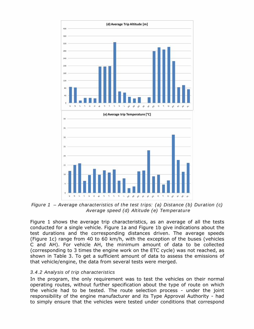
Figure 1 – Average characteristics of the test trips: (a) Distance (b) Duration (c)

Average speed (d) Altitude (e) Temperature Figure 1 shows the average trip characteristics, as an average of all the tests conducted for a single vehicle. Figure 1a and Figure 1b give indications about the test durations and the corresponding distances driven. The average speeds (Figure 1c) range from 40 to 60 km/h, with the exception of the buses (vehicles C and AH). For vehicle AH, the minimum amount of data to be collected (corresponding to 3 times the engine work on the ETC cycle) was not reached, as shown in Table 3. To get a sufficient amount of data to assess the emissions of that vehicle/engine, the data from several tests were merged.

3.4.2 Analysis of trip characteristics In the program, the only requirement was to test the vehicles on their normal operating routes, without further specification about the type of route on which the vehicle had to be tested. The route selection process - under the joint responsibility of the engine manufacturer and its Type Approval Authority - had to simply ensure that the vehicles were tested under conditions that correspond

to their real usage: for instance, a city bus had to be tested on a city trip. The only reporting mechanism regarding the route characteristics included the average trip characteristics shown in Figure 1. A more detailed analysis of the test route characteristics was conducted for a few cases: the objective was to highlight how the trip composition and the speed distribution could vary as a function of the type of vehicle. Several cases, chosen to be representative of the vehicle types and operations in the fleet, were used:

Large trucks, (Vehicles A, B, F, G, P) Medium truck, (Vehicle X, S) Bus, Intercity operation (C)

Idle City Rural Highway

VEH_A_TEST5 32% 14% 10% 43% VEH_B_TEST2 28% 28% 19% 25% VEH_F_TEST3 11% 44% 16% 29% VEH_G_TEST2 19% 39% 18% 23% VEH_P_TEST4 6% 32% 39% 24% VEH_X_TEST1 9% 34% 30% 27% VEH_S_TEST3 9% 36% 31% 25%

Table 4 - Examples of trip compositions – Share of idling, city, rural and motorway operation

City Rural Highway VEH_A_TEST5 21% 15% 63% VEH_B_TEST2 39% 26% 35% VEH_F_TEST3 49% 18% 33% VEH_G_TEST2 49% 22% 29% VEH_P_TEST4 34% 41% 25% VEH_X_TEST1 37% 33% 29% VEH_S_TEST3 39% 34% 27%

Table 5 Examples of trip compositions – Share city, rural and motorway operation excluding idling Table 4 shows the trip composition determined from the speed following ranges:

Less than 50 km/h: city; Between 50 and 70 km/h: rural; Greater than 70 km/h: highway.

Figure 2 (through the intercept on the Y axis) shows that some vehicles (A, B) included long sections with idling, representing more than 30% of the total test data. In the first case (A), this idling was due to the decision not to interrupt the measurements. In the second case (B), the idling represented the real operation of the vehicle, i.e. an asphalt truck unloading and waiting on a construction site. For these vehicles, it must be noted that the non-idling data represented several hours and that they met without problem the criterion regarding the minimum trip duration (i.e. at least 3 times the engine work on the ETC), as shown by the results in Table 3.

0%

10%

20%

30%

40%

50%

60%

70%

80%

90%

100%

0 10 20 30 40 50 60 70 80 90 100

Freq

uency

Speed [km/h]

Examples of Cumulative Speed Distributions

VEH_A_TEST5

VEH_B_TEST2

VEH_F_TEST3

VEH_G_TEST2

VEH_P_TEST4

VEH_X_TEST1

VEH_S_TEST3

Figure 2 – Example of cumulative speed distributions

The effect of the trip composition upon the engine emissions evaluation is discussed more in detail in sections 4.4.5 (in general) and 4.5.2 (for in the case of the idling operation). From the analysis conducted in the present section, it appears already that the average test route characteristics (as presented in section 3.4.1) are not detailed enough to characterize the test route and the driving conditions. To make the test evaluation easier and to better report under which conditions a given vehicle is driven, it would be needed to develop other indicators. This shall include the share of idling time (with respect to the total test duration) and could include for instance:

The cumulative speed distributions to allow a quick verification of the driving conditions, e.g. to determine for instance the share of city, rural and highway operation;

The reporting of the GPS trace on a map, together with the associated driving conditions.

3.5 Data handling procedures and tools

3.5.1 Test data The parameters that had to be recorded are listed in Table 6. The unit mentioned is the reference unit whereas the source column shows the types of methods that were used.

3.5.2 Time alignment The test data listed in Table 6 are split in 3 different categories:

Category 1: Gas analyzers (THC, CO, CO2, NOx concentrations);

Category 2: Exhaust flow meter (Exhaust mass flow and exhaust temperature);

Category 3: Engine (Torque, speed, temperatures, fuel rate, vehicle speed from ECU).

The time alignment of each category with the other categories may be verified by finding the highest correlation coefficient between two series of parameters. All the parameters in a category shall be shifted to maximize the correlation factor. The following parameters may be used to calculate the correlation coefficients: To time-align:

Categories 1 and 2 (Analyzers and EFM data) with category 3 (Engine data): the vehicle speed from the GPS and from the ECU.

Category 1 with category 2: the CO2 concentration and the exhaust mass flow;

Category 2 with category 3: the CO2 concentration and the engine fuel flow.

Parameter Unit Source THC concentration (1) ppm Analyser CO concentration (1) ppm Analyser NOx concentration (1) ppm Analyser CO2 concentration (1) ppm Analyser CH4 concentration (1) (2) ppm Analyser Exhaust gas flow kg/h EFM Exhaust temperature °K EFM Ambient temperature(3) °K Sensor Ambient pressure kPa Sensor Engine torque N.m ECU or Sensor Engine speed rpm ECU or Sensor Engine fuel flow g/s ECU or Sensor Engine coolant temperature °K ECU or Sensor Engine intake air temperature(3) °K Sensor Vehicle ground speed km/h ECU and GPS Vehicle latitude degree GPS Vehicle longitude degree GPS

(1)Measured or corrected to a wet basis (2)Gas engines only (3)Use the ambient temperature sensor or an intake air temperature sensor

Table 6 - Test parameters

3.5.3 EMROAD© Reporting templates and an automated data analysis have been developed to ensure that all the calculations (of mass, distance specific and brake specific emissions) and verifications were done in a consistent way throughout the program. The standardised reporting templates included, for every road test:

Second by second test data for all the mandatory test parameters; Second by second calculated data (mass emissions, distance, fuel and

brake specific);

Improved time alignment procedures between the different families of measured signals (analysers, EFM, engine);

Data verification routines, using the duplication of measurement principle, to check for instance the directly measured exhaust flow against the calculated one;

Averages and integrated values (mass emissions, distance, fuel and brake specific).

The calculations and the data verifications were carried out using EMROAD©.

3.5.4 Data consistency checks Three types of (post-test) data consistency checks have been developed. They are complementing the 'normal' verifications made during a test, e.g. the zero-span of the gas analysers. Type 1 The first was a very simple and automated routine checking:

The presence of all the mandatory parameters; The existence of values outside the instrument ranges or outside normally

expected ranges (e.g. vehicle speed negative or greater than 120 km/h); Type 2 The second is a verification of the exhaust mass flow and the emissions data. It makes use of a correlation between the fuel rate -calculated from the emissions and the exhaust mass flow, using the carbon balance equations in the ISO standard (R11). A linear regression was performed for the measured and calculated fuel rate values. The method of least squares was used, with the best fit equation having the form: y = mx + b where: y = Calculated fuel flow [g/s] m = slope of the regression line x = Measured fuel flow [g/s] b = y intercept of the regression line The slope (m) and the coefficient of determination (r²) were calculated for each regression line. This analysis was performed in the range [15% of the maximum value - maximum value] and at a frequency greater or equal to 1 Hz. The results of the linear regressions (slope (m) and the coefficient of determination (r²)) were calculated for all tests and vehicles. The r² results may be qualified as excellent in most cases. For the value of the slope (m), different situations occurred, depending on the uncertainty on the ECU fuel rate. For low uncertainties, the calculated fuel rate was usually within ±5% of the measured. For high uncertainties (or even unknown ECU fuel rate), the verification on the slope could not be done as evidenced by slope values outside the range [0.8 - 1.2].

Type 3 The last verification that was developed looks at the consistency of the ECU torque values with respect to the declared full-load curve. All the submitted data passed with the 'Type 1' verification. The results of the Type 2 data consistency checks are summarised in Table 7.

Margin % of tests within the

range

Slope m ±5% 37.84

Slope m ±10% 54.05

Slope m ±20% 64.86

r2 > 0.95 97.30

r2 > 0.98 54.05

r2 > 0.99 35.14 Table 7 - Results of the 'Type 2' verification: percentage of vehicles fulfilling pre-

set criteria for the slope m and the coefficient of determination

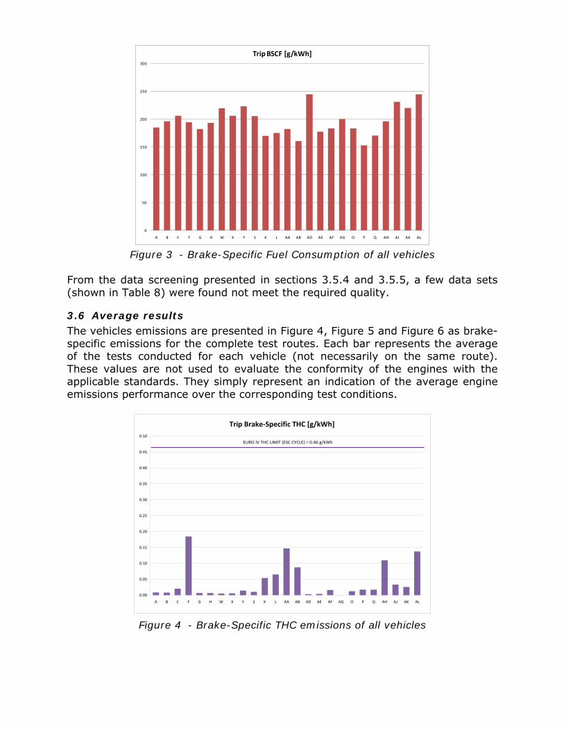
3.5.5 Plausibility of BSFC values The following figure represents the average brake-specific fuel consumption (BSFC) of the vehicles tested in the Pilot Program. The BSFC results are calculated from the PEMS data: the fuel consumption is obtained from the emissions and exhaust mass flow data whereas the work is calculated from the ECU torque and speed signals. The results shows that some BSFC values are anomalous (150-160 grams of fuel per kWh) when compared to the ‘normal’ values observed for such engines (from 190 g/kWh). The results from section 3.5.4 were helpful to understand which test parameter is likely to cause such anomalous values: ECU torque, exhaust flow measurement, emissions or all. These findings are summarised in Table 8. Parameter / Verification Number of cases Exhaust Flow / Type 2 1 Emissions / Zero-Span 1 ECU engine torque / Full load curve 1 At least 2 of the above 1

Table 8 - Number of cases per cause for non-plausible BSFC values

0

50

100

150

200

250

300

A B C F G H W X Y S K L AA AB AD AE AF AG O P Q AH AJ AK AL

Trip BSCF [g/kWh]

Figure 3 - Brake-Specific Fuel Consumption of all vehicles

From the data screening presented in sections 3.5.4 and 3.5.5, a few data sets (shown in Table 8) were found not meet the required quality.

3.6 Average results The vehicles emissions are presented in Figure 4, Figure 5 and Figure 6 as brake-specific emissions for the complete test routes. Each bar represents the average of the tests conducted for each vehicle (not necessarily on the same route). These values are not used to evaluate the conformity of the engines with the applicable standards. They simply represent an indication of the average engine emissions performance over the corresponding test conditions.

Trip Brake‐Specific THC [g/kWh]

0.00

0.05

0.10

0.15

0.20

0.25

0.30

0.35

0.40

0.45

0.50


EURO IV THC LIMIT (ESC CYCLE) = 0.46 g/kWh

Figure 4 - Brake-Specific THC emissions of all vehicles

Trip Brake‐Specific CO [g/kWh]

0.00

0.25

0.50

0.75

1.00

1.25

1.50

1.75

2.00

2.25

2.50

2.75

3.00

3.25

3.50

3.75

4.00

4.25

4.50


EURO V CO LIMIT (ETC CYCLE) = 4.0 g/kWh

Figure 5 - Brake-Specific CO emissions of all vehicles

Trip Brake‐Specific NOx [g/kWh]

0.00

1.00

2.00

3.00

4.00

5.00

6.00

7.00

8.00

9.00

10.00


EURO IV NOx LIMIT (ETC CYCLE) = 3.5 g/kWh

Figure 6 - Brake-Specific NOx emissions of all vehicles (NB: EURO IV and V

vehicles together)

4 In-Service Conformity Emissions Evaluation

4.1 Introduction Following the recommendations of the EU-PEMS project preceding the Pilot Program, two data evaluation methods were retained as candidates. Their feasibility in view of ISC has been assessed throughout the different phases of the work:

The "control-area methods", use only that part of the data for which the operating points are for a minimum period of uninterrupted time within a predetermined control area; thus forming a sequence of consecutive points within this control area. Each sequence is also called 'event'. The US-NTE (Not To Exceed) method - already established as a standard for in-use on-highway testing in the United States - falls into this category.

The "averaging window methods" that use all the operation data are based

on a moving averaging window whose size is based on a reference quantity (typically the engine work or the engine CO2 mass emissions measured with the engine's certification cycle).

4.2 Control area methods

4.2.1 Introduction The engine "operating points" are defined as pairs of engine speed and torque values, typically read from the vehicle ECU when testing with PEMS. The in-service brake-specific emissions are calculated when the engine operating points belong to the control area for a minimum duration, also known as the "minimum sampling rule". An "event" can be defined as a sequence of data whose operating points belong to the control area for at least the duration of the minimum sampling rule (at least 30 consecutive seconds in the US-NTE). For each event, a brake-specific emissions value is calculated, dividing the mass emissions by the event work. The calculations in this study were carried out with the US-NTE area and the default minimum sampling rule set to a duration of 30 seconds. The speed boundaries of the control area (filled in with a yellow color in Figure 7), are obtained from the engine speeds lown and highn , whereas the power boundary is

set to 30% of maximum engine power and the torque boundary to 30% of maximum torque, where:

- highn is determined by calculating 70 % of the declared maximum net power. The highest engine speed where this power value occurs on the power curve is defined as highn .

- lown is determined by calculating 50 % of the declared maximum net

power. The lowest engine speed where this power value occurs on the power curve is defined as lown .

The control area low speed boundary is obtained from:

Equation 1 ( )lowhighlowlow nnnNTE −+= 15.0

US-NTE (Not To Exceed)

Engine speed (rpm)

E

ngin

e to

rque

(Nm

)0.5xPmax

0.7xPmax

Pmax

0% 25% 50% 75% 100%

Definitions: n low = 0% (at 0.5xPmax) n high = 100% (at 0.7xPmax) n (limit NTE)=15%

A speed=25% B speed=50% C speed=75%

25%

50%

75%

100%

2004-01-13 AE

n low n high

15%

0.3xMmax

0.3xPmax

= NTE-control area

A B C

Applicable at:-Altitudes<5500 ft-Normal operating conditions

Figure 7 Definition of the US-NTE area

An engine operating point is retained for the calculation when it fulfils the following criteria:

Rule1: Engine speed ≥ lowNTE Rule 2: Engine power ≥ 30% of Engine maximum power Rule 3: Engine torque ≥ 30% of Engine maximum torque Rule 4: The operating point is part of a set of at least 30 seconds of data

which lay always in the control area (minimum sampling rule). In the United States official rules (Code of Federal Regulations Paragraph 86.007-11 and Paragraph 86.1370-2007). Other criteria (not used for the evaluation in section 4.2.2) are applied on the engine condition.

4.2.2 Effect of control are methods on data sets The amount of data “captured” with respect to the total of data is illustrated for one vehicle and one route in Figure 8, which shows the vehicle speed-time trace and the control area events are plotted. For the complete trip shown in Figure 14, the amount of data captured corresponding to Figure 8 is 14%. The same analysis was conducted for all the vehicles tested in the Pilot Program. The results are presented in Figure 9 and show that:

A limited amount of the total test data can be used (10 to 20%), with the exception of the fully loaded trucks operated on the motorway with cruise control (40%);

The control area methods do not provide any data when the vehicles are tested under dynamic conditions: typically, vehicles operated with stop and go such as (See the first part of the trip on Figure A1);

The event durations are rather short, i.e. in the range of 1 to 2 minutes maximum.

Figure 8 - Example of data covered by the control area method: truck with 50%

of its max. payload on city and motorway routes

0

10

20

30

40

50

60

70

80

90

100

Percentage of Total Test Time in NTE Area

Figure 9 - Percentage of test data in the control area using the US-NTE

calculation settings (Minimum sampling rule of 30s)

4.2.3 Conclusions on the control area methods The control area methods (US-NTE type) have the following practical drawbacks:

They make only use of a small fraction of the data (10 to 20% of the total test data for under common European driving conditions);

The emissions calculations are made for very short durations (30 seconds to 2 minutes) and the resulting emissions exhibit scatter and are difficult to interpret;

Finally, the measurement of PM mass emissions would be extremely challenging, as the principle of the control area methods requires the measurement of PM mass changes for durations as short as 30 seconds: the technical feasibility of such a measurement is more than uncertain for the future low-PM emissions engines equipped with Diesel Particle Filters (DPF).

4.3 Averaging window methods

4.3.1 Introduction For the averaging window methods, the emissions are averaged over windows whose common characteristic is the engine work or its CO2 mass emissions on a reference certification transient cycle. The reference quantity, i.e. the engine work or its CO2 mass emissions, is easy to calculate or to measure:

In the case of work: from the basic engine characteristics (Maximum power), the duration and the average power of the reference transient certification cycle;

In the case of the CO2 mass: from the engine CO2 emissions on its certification cycle.

The first average value is obtained between the first data point and the data point for which the reference quantity is reached. The calculation is then moving, with a time increment equal to the data sampling frequency (at least 1Hz for the gaseous emissions). The averaging window method is a moving averaging process, making use of a reference quantity obtained from the engine characteristics and its performance on the reference type approval transient cycle.

Figure 10 - Principle of the averaging window method

The reference quantity fixes the character of the averaging process (i.e. the duration of the windows). The possibility to use a CO2 mass instead of engine work was investigated to possibly simplify the whole procedure: it could avoid the recording of engine torque and speed from the ECU. The equivalency between these two approaches is discussed in section 4.5.3.

4.3.2 Averaging window calculations The calculation principle is the following: the data set is partitioned in sub set whit length determined to match the engine CO2 mass or work measured over the reference laboratory transient cycle; for each of the above defined sub set we compute the engine emissions. The moving average calculations are conducted with a time increment tΔ equal to the data sampling period. In the following the sub set will be referred to as “averaging window”. The duration )( ,1,2 ii tt − of the ith averaging window is determined by:

For the CO2 mass based method: refCOiCOiCO mtmtm ,2,12,22 )()( ≥−

Where: • - )( ,2 ijCO tm is the CO2 mass measured between the test start and time tj,i, g;

• is the CO2 mass determined for the ETC, g; • t2,i shall be selected such as: • )()()()( ,12,22,2,12,22 iCOiCOrefCOiCOiCO tmtmmtmttm −≤<−Δ−

Where tΔ is the data sampling period, equal to 1 second or less. In each window, the CO2 mass is calculated integrating the instantaneous emissions. For the Work based method:

refii WtWtW ≥− )()( ,1,2

Where: • - )( ,ijtW is the engine work measured between the start and time tj,i, kWh;

• - refW is the engine work for the ETC, kWh.

• t2,i shall be selected such as: )()()()( ,1,2,1,2 iirefii tWtWWtWttW −≤<−Δ−

Where tΔ is the data sampling period, equal to 1 second or less. Any section of invalidated data for:

The periodic verification of the instruments and/or after the zero drift verifications;

The data outside the applicable conditions (e.g. altitude or cold engine); shall not be considered for the calculation of the work / CO2 mass and the

emissions of the averaging window. The mass emissions (g/window) shall be determined using the emissions calculation formula for raw exhaust gas, as described in the European Directives 2005/55/EC-2005/78/EC in Annex III, Appendix 2, Section 5.

Work [kWh]

Emission

s [g]

)( ,2 ttW i Δ− )( ,2 itW)( ,1 itW

refii WtWtW ≥− )()( ,1,2

refii WtWttW <−Δ− )()( ,1,2

)( ,2 itm

)( ,1 itm

m

Work based method

Figure 11 - Work based method

CO2 Emissions [kg]

Emission

s [g]

)( ,2 itm

)( ,1 itm

m

CO2 mass based method

refCOiCOiCO mtmttm ,2,12,22 )()( <−Δ−

refCOiCOiCO mtmtm ,2,12,22 )()( ≥−

)( ,22 ttm iCO Δ− )( ,22 iCO tm)( ,12 iCO tm

Figure 12 - CO2 based method

4.3.3 Calculation of the specific emissions For the Work based method: The specific emissions egas (g/kWh) are calculated for each window and each pollutant in the following way:

ref

gas Wme =

Where:

• m is the mass emission of the component, g/window • Wref is the engine work for the ETC, kWh

4.3.4 Calculation of the conformity factors The conformity factors are calculated for each individual window and each individual pollutant in the following way: For the CO2 mass based method:

C

I

CFCFCF =

With refCO

I mmCF

,2

= (in service ratio) and refCO

LC m

mCF

,2

= (certification ratio)

Where:

• m is the mass emission of the component, g/window • refCOm ,2

is the engine CO2 mass measured on the ETC or calculated from:

refrefCO WBSFCm ⋅⋅= 172,3,2

Lm is the mass emission of the component corresponding to the applicable limit on the ETC, g For Work based method:

LeCF =

Where:

• e is the brake-specific emission of the component, g/kWh • L is the applicable limit, g/kWh

4.3.5 Maximum allowed conformity factor For the CO2 mass based method: The valid windows are the windows whose duration does not exceed the threshold duration calculated from:

maxmax 2.0

3600P

WD ref

⋅⋅=

Where:

• maxD if the maximum allowed window duration, s • maxP is the maximum engine power, kW

For the Work based method: The valid windows are the windows whose average power exceeds the power threshold of 20% of the maximum engine power.

4.3.6 Calculation steps To calculate the conformity factors, the following steps have to be followed: Step 1: Additional and empirical time-alignment, as described in section 3.5.2. Step 2: Invalid data: Exclusion of data points not meeting the applicable ambient and altitude conditions: for the pilot program, these conditions (on engine coolant temperature, altitude and ambient temperature) were defined in the Directive 2005/78/EC [R3]. Step 3: Moving and averaging window calculation, excluding the invalid data. If the reference quantity is not reached, the averaging process restarts after a section with invalid data. Step 4: Invalid windows: Exclusion of windows whose power is below 20% of maximum engine power. Step 5: Selection of the reference value from the valid windows: 90% cumulative percentile.

Steps 2 to 5 apply to all regulated gaseous pollutants (and shall apply to PM in the future).

4.4 Results with the averaging window method

4.4.1 Introduction The emissions are presented as ‘Conformity Factors’ (as defined in Section 4.3.4), to compare the EURO IV and V engines on the same scale. The emissions are averaged using the principle described in Section 4.3.2 and the engine work on the European Transient Cycle (ETC) as a reference. Most of the vehicles were tested several times but the results in sections 4.4.2 and 4.4.3 are presented for one (randomly selected) test.

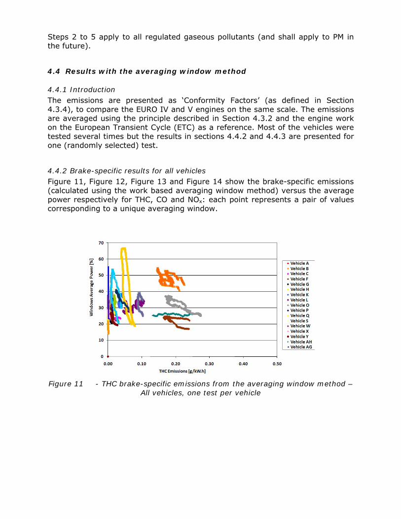
4.4.2 Brake-specific results for all vehicles Figure 11, Figure 12, Figure 13 and Figure 14 show the brake-specific emissions (calculated using the work based averaging window method) versus the average power respectively for THC, CO and NOx: each point represents a pair of values corresponding to a unique averaging window.

Figure 11 - THC brake-specific emissions from the averaging window method –

All vehicles, one test per vehicle

Figure 12 - CO brake-specific emissions from the averaging window method –

All vehicles, one test per vehicle

Figure 13 - NOx brake-specific emissions from the averaging window method –

EURO IV vehicles, one test per vehicle (Limit on ETC cycle, 3.5 g/kWh)

Figure 14 - NOx brake-specific emissions from the averaging window method –

EURO V vehicles, one test per vehicle (Limit on ETC cycle, 2 g/kWh)

4.4.3 NOx Conformity Factors for all vehicles The results presented in section 4.4.2 for the NOx brake-specific emissions are show respectively the numbers obtained for the EURO IV (Figure 13) and the EURO V (Figure 14) vehicles. To compare EURO IV and EURO V vehicles on the same scale, the results are expressed as conformity factors. Two colours are used: orange for EURO IV and green for EURO V.

Figure 15 - NOx conformity factors from the averaging window method – EURO

IV and V vehicles, one test per vehicle From Figure 15, the following observations can be made:

The figure does not reflect the density of the data; A large share of averaging window lies in the range 20%-40% of the

maximum engine power. The shape of the individual ‘clouds’ is give information on the behaviour of

the engine systems: an anomalous increase of brake specific emission at low power can be caused by average windows either including a significant portion of idling data and/or poorly functioning after-treatment systems;

The vehicles/engines that would fail clearly on the right side and outside the main ‘cloud’.

Figure 16 shows the same results as Figure 15 expressed in g/h instead of g/kWh (or its corresponding conformity factor). The increasing brake-specific emissions at low engines loads presented in Figure 15 do not necessarily correspond to increasing time-specific emissions.

Figure 16 - Time-specific NOx emissions from the averaging window method –

EURO IV and V vehicles, one test per vehicle

4.4.4 Test to test variability The nature of on-road testing includes the variability of the testing conditions generated by the changes of the vehicle payload, the traffic and the driver, for a given test route. The variability is expected to be even larger if different test routes are driven. The first case (illustrated with the case of vehicle A) shows how the (averaging window) NOx emissions vary for the same vehicle driven on different test routes (7) with different payloads. The second case (illustrated with the case of vehicle O) shows how the (averaging window) NOx emissions vary for the same vehicle driven several times (4) on the same route and with the same payload. Table 9 and Table 10 show the main pass-fail results. More interestingly, the histograms of the NOx emissions show that in some cases bi-modal distributions may be obtained. This is the case for test #4, or – to a lower

extent – for test #3 for vehicle A. These results also confirm that the better representativeness of the engine emissions (which is a strong indicator of the engine emissions performance and therefore its potential conformity) is obtained with the 90% cumulative percentile. The data in Figure 19 shows for some vehicles a large difference between the maximum emissions and the 90% cumulative percentile, which confirms that the 90% cumulative percentile could be a better indicator of the engine emissions performance. The 10% highest emissions may in some cases be a result of the averaging process and leading to windows including a large share of idling and causing higher brake-specific emissions.

0

500

1000

1500

2000

2500

3000

3500

0 10 20 30 40 50 60 70

Num

ber o

f events

Window Average Power [%]

Test 1

Test 2

Test 3

Test 4

Test 5

Test 6

Test 7

Figure 17 - Histograms of NOx conformity factors and average power

calculated from the averaging window method – Vehicle A, all tests

0

500

1000

1500

2000

2500

3000

3500

0.00 0.50 1.00 1.50 2.00 2.50

Num

ber o

f events

NOx Conformity Factors

Test 1

Test 2

Test 3

Test 4

0

200

400

600

800

1000

1200

1400

1600

1800

0 10 20 30 40 50 60 70

Windows Average Power [%]

Num

ber o

f events

Test 1

Test 2

Test 3

Test 4

Figure 18 - Histogram of NOx conformity factors and average power calculated

from the averaging window method – Vehicle O, all tests

Test 1 2 3 4 5 6 7 Max NOx CF 1.44 1.45 1.61 1.50 1.70 1.43 1.29 90% NOx CF 1.15 1.34 1.17 1.43 1.65 1.40 1.25 Min. Window Power 24 21 12 14 11 23 18 Max. Window Power 50 35 59 54 60 34 65 Data Coverage Index

100 100 100 100 100 100 100

Percentage of valid windows

100 100 100 100 100 100 100

Table 9 - Vehicle A – Test-to-test repeatability using the main results of the pass-fail analysis

Test 1 2 3 4 Max NOx CF 1.26 1.34 1.22 1.55 90% NOx CF 1.16 1.18 1.10 1.03 Min. Window Power 30 30 31 31 Max. Window Power 51 48 47 48 Data Coverage Index

100 100 100 100

Percentage of valid windows

100 100 100 100

Table 10 - Vehicle O – Test-to-test repeatability using the main results of the pass-fail analysis

0.00

0.25

0.50

0.75

1.00

1.25

1.50

1.75

2.00

2.25

2.50

2.75

3.00

3.25

3.50

NOx C

onform

ity Factor

Maximum

Percentile 95

Percentile 90

Percentile 85

Percentile 80

Percentile 50

EURO V engines

Figure 19 - Distribution of NOx conformity factors – All vehicles, one tests

4.4.5 Case studies The present section describes in detail results obtained for a few cases of vehicles and for operating conditions that are typical for the European vehicle market and operating conditions and in particular:

CS1: A large truck, (Vehicle O/P, SCR, EURO V) with high and low payload (mixed driving conditions);

CS2: A medium truck, (Vehicle X, SCR, EURO IV), half loaded, tested under mixed driving conditions;

CS3: An 'intercity bus', (Vehicle C, SCR, EURO IV) i.e. a bus tested under mixed driving conditions;

CS4: A large construction (asphalt) truck (Vehicle B, SCR, EURO IV) whose operation includes multiple loads and long idling durations.

The trip composition for these vehicles is presented in section 3.4.2. The figures show the vehicle speed and the main averaging window results as function of time, i.e.:

The average window power (a); The NOx conformity factors (a); The distribution/histogram of the NOx conformity factors (b).

Table 11 presents:

The main pass-fail emissions results; The window coverage to indicate which windows are below the proposed

threshold of 20% of maximum engine power; The data coverage index to indicate which sections of the data are not

included in any of the windows.

Vehicle O P X B C Test 3 3 1 3 3 Maximum NOx CF 1.22 1.51 1.20 1.32 1.38 90% C.P. NOx CF 1.10 1.48 1.13 1.22 1.32 Min. Window Power 31% 25% 20% 12% 18% Max. Window Power 47% 33% 29% 46% 28% Data Coverage Index 100 100 100 100 100 Percentage of valid windows

100 100 100 100 100

Table 11 - Main Pass-Fail results for case study vehicles The following observations can be made:

The effect of the vehicle payload (or power to mass ratio) upon the average power may be observed with the results from vehicles O and P: a lower power to mass ratio (high payload, vehicle O) corresponds to higher average operating powers and lower brake-specific emissions (i.e. conformity factor);

The route composition has an influence upon the thermal history of the engine system. Results from vehicle X are obtained on a test route where the first part is performed at low engine power, which results in longer warm-up time for the engine and the after treatment system, hence increasing the emission in the first section of the test. On the contrary, the tests conducted for vehicles O and P were less challenging in that respect, as the vehicle was taken to the motorway only after a short city-rural section.

The figures presented for each case also show:

Which average emissions (windows) are excluded by the power threshold rule - when applicable - or the 90% cumulative percentile: these exclusions are evidenced on the top figures (labelled a), by the purple and orange bars, respectively for the power threshold and the cumulative percentile.

The probability of the single data points to belong to averaging windows, as a consequence of the above exclusions, shown in the bottom figures (labelled b). In the latter figures, the data points having a probability equal to zero are the ones excluded for cold start.

The (b) figures illustrate a feature of the moving averaging window methods: the data points do not have equal probabilities to belong to a window. For instance, the first 'valid' (i.e. not excluded for cold start or altitude) data point can only

belong to the first 'valid' (i.e. above the power threshold or not belonging to the highest 10%) window.

0.0

0.5

1.0

1.5

2.0

2.5

3.0

0 1000 2000 3000 4000 5000 6000 7000

Time [s]

‐100

‐80

‐60

‐40

‐20

0

20

40

60

80

100

NOx 90CP EXCLUSION NOx CONFORMITY FACTOR POWER EXCLUSION VEHICLE SPEED [km/h, RIGHT]

(a)

0

10

20

30

40

50

60

70

80

0 1000 2000 3000 4000 5000 6000 7000

Time [s]

‐100

‐80

‐60

‐40

‐20

0

20

40

60

80

100

DATA POINTS WINDOW PROBABILITY VEHICLE SPEED [km/h, RIGHT]

(b) Figure 20 - Vehicle O, Test 3 (Large truck, full load) - Pass fail results (a) NOx conformity factor and invalid windows – (b) Data points in-window probability

0.0

0.5

1.0

1.5

2.0

2.5

3.0

0 1000 2000 3000 4000 5000 6000 7000

Time [s]

‐100

‐80

‐60

‐40

‐20

0

20

40

60

80

100


(a)

0

10

20

30

40

50

60

70

80

90

100

0 1000 2000 3000 4000 5000 6000 7000

Time [s]

‐100

‐80

‐60

‐40

‐20

0

20

40

60

80

100


(b)

Figure 21 - Vehicle P, Test 3 (Large truck, half load) - Pass fail results (a) NOx conformity factor and invalid windows – (b) Data points in-window probability

0.0

0.5

1.0

1.5

2.0

2.5

3.0

0 2000 4000 6000 8000 10000 12000

Time [s]

‐100

‐80

‐60

‐40

‐20

0

20

40

60

80

100


(a)

0

5

10

15

20

25

30

35

40

45

50

0 2000 4000 6000 8000 10000 12000

Time [s]

‐100

‐80

‐60

‐40

‐20

0

20

40

60

80

100


(b)

Figure 22 - Vehicle X, Test 1 (Medium truck, half loaded) - Pass fail results (a) NOx conformity factor and invalid windows – (b) Data points in-window

probability

0.0

0.5

1.0

1.5

2.0

2.5

3.0

0 2000 4000 6000 8000 10000 12000

Time [s]

‐100

‐80

‐60

‐40

‐20

0

20

40

60

80

100


(a)

0

5

10

15

20

25

30

35

40

45

50

0 2000 4000 6000 8000 10000 12000

Time [s]

‐100

‐80

‐60

‐40

‐20

0

20

40

60

80

100


(b)

Figure 23 - Vehicle B, Test 3 (Construction truck, variable payloads, long idling periods) - Pass fail results (a) NOx conformity factor and invalid windows – (b)

Data points in-window probability

0.0

0.5

1.0

1.5

2.0

2.5

3.0

0 2000 4000 6000 8000 10000 12000 14000

Time [s]

‐100

‐80

‐60

‐40

‐20

0

20

40

60

80

100


(a)

0

10

20

30

40

50

60

0 2000 4000 6000 8000 10000 12000 14000

Time [s]

‐100

‐80

‐60

‐40

‐20

0

20

40

60

80

100


(b)

Figure 24 - Vehicle C, Test 3 (Intercity Bus) - Pass fail results (a) NOx conformity factor and invalid windows – (b) Data points in-window probability

4.5 Settings of the averaging window method

4.5.1 Power threshold The reasons for the introducing the power threshold were:

To find a solution to account for increasing brake-specific emissions at low power (illustrated in Figure 13), which in many cases is caused by the inclusion of long idling periods in the averaged values.

To evaluate windows whose power is as close as possible to the power of the transient certification test cycle, in view of the engine conformity evaluation.

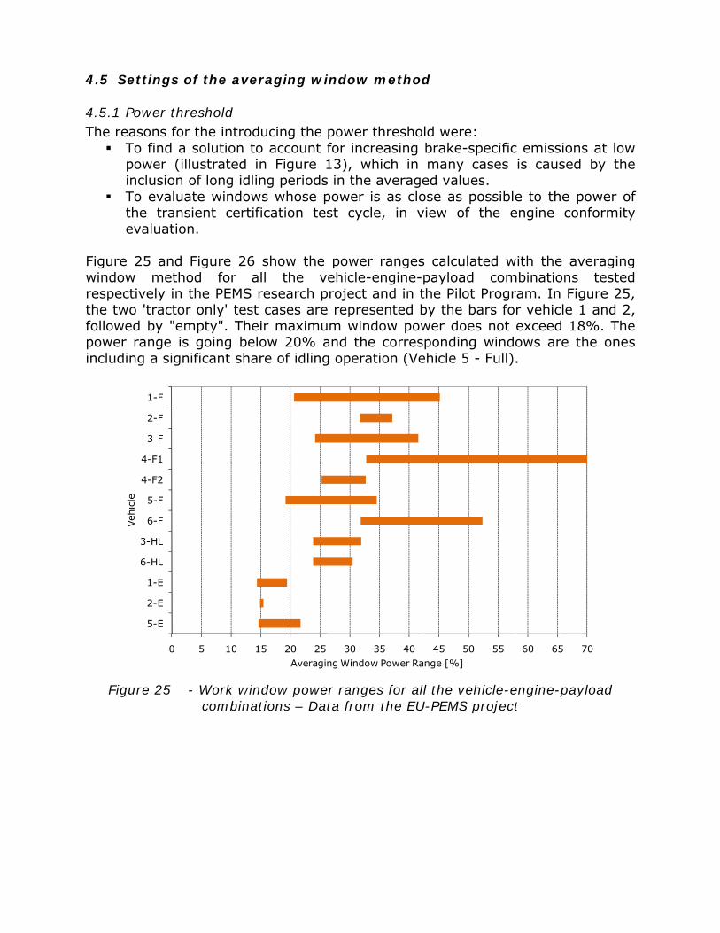
Figure 25 and Figure 26 show the power ranges calculated with the averaging window method for all the vehicle-engine-payload combinations tested respectively in the PEMS research project and in the Pilot Program. In Figure 25, the two 'tractor only' test cases are represented by the bars for vehicle 1 and 2, followed by "empty". Their maximum window power does not exceed 18%. The power range is going below 20% and the corresponding windows are the ones including a significant share of idling operation (Vehicle 5 - Full).

0 5 10 15 20 25 30 35 40 45 50 55 60 65 70

1-F

2-F

3-F

4-F1

4-F2

5-F

6-F

3-HL

6-HL

1-E

2-E

5-E

Averaging Window Power Range [%]

Veh

icle

Figure 25 - Work window power ranges for all the vehicle-engine-payload

combinations – Data from the EU-PEMS project

0 5 10 15 20 25 30 35 40 45 50 55 60 65 70

Veh A v.L.(Test3)

Veh B v.L.(Test2)

Veh C

Veh G

Veh H

Veh O

Veh Q

Veh W

Veh X

Veh Y

Veh AG

Veh F

Veh P

Veh A v.L. (Test2)

Veh B v.L. (Test2)

Veh K

Veh L

Figure 26 - Averaging window power ranges for vehicle-engine-payload combinations – Data from the EU-PEMS Pilot Program - (V.L = Vehicle with

variable payload, i.e. several payloads during a single test)

4.5.2 Effect of idling For some of the vehicles tested during this program, the data included large sections in which the vehicle was idling. In some situations, vehicle idling cannot be avoided during a test: it is part of the real vehicle operation (construction) and/or it is caused by traffic congestion. Such results were illustrated for vehicle B (construction truck) in section 4.4.5. The effect of idling upon emissions is shown in Figure 28 for vehicle A: the exhaust temperature may decrease down to a temperature where the SCR after-treatment systems have a low efficiency or are even shut-down. Figure 28 also shows the engine coolant temperature throughout the entire test and highlights that – as the coolant temperature remains above 70°C - the engine remains 'hot' under the definition of the laboratory engine test. To understand how the data evaluation method deals with such testing/driving situations, the effect of idling upon the engine behaviour and the averaged emissions is illustrated for three tests conducted with vehicle A, in Figure 27. The results were analysed with the averaging window method respectively for the work based calculations (a), CO2 mass based (b) and limited idling durations (c). For the latter, the calculations were carried out using the following principle: if the vehicle started to idle for more than 2 minutes, the data corresponding to the idling following the first 2 minutes was discarded. For instance, if the vehicle is idling for 10 minutes, the data corresponding to the last 8 minutes was marked as invalid and not included in the averaging calculations.

Figure 28 shows the engine coolant and exhaust temperatures throughout an entire test. Both the coolant and the exhaust temperature decrease significantly during idling. The coolant temperature remains greater than 70°C: the engine remains 'hot' according to the definition of a laboratory test. The decrease of the exhaust temperature below 250°C is affecting the efficiency of the SCR after-treatment system, as evidenced by the NOx concentrations in the parts of the test following the idling phases.

Method Test 3 4 5

Work based Max NOx CF 1.49 1.44 1.63 90% NOx CF 1.17 1.26 1.25

CO2 mass based Max NOx CF 1.54 1.49 1.58 90% NOx CF 1.25 1.35 1.33

Work based with maximum idling duration (2 min.)

Max NOx CF 1.24 1.29 1.35

90% NOx CF 1.16 1.20 1.23

Table 12 - Vehicle A – Vehicle idling: Effect of different calculation methods upon the representative emissions

The results showed in Table 12 that the 3 methods (work based, with 20% power threshold, and the limitation of the idling duration) lead to close results in terms of representative emissions values. More details on the results provided by the methods are presented in Figure 27.

(a)

(b)

(c)

Figure 27 - Average window power (%) versus conformity factor, vehicle A, 3 tests - (a) work based (b) CO2 mass based (c) work based with maximum idling

duration of 2 minutes

(a)

(b) Figure 28 - Vehicle Speed (a) Engine coolant and exhaust (b) temperatures

changes throughout a test including a long idling section: Vehicle A, Test 3

4.5.3 Reference quantity: work or CO2 mass? Not to rely on the torque data broadcasted on the vehicle networks by the Engine Control Units and whose accuracy is uncertain, the possibility to use another reference quantity for the moving average was investigated. To keep a strong link with the certification transient cycle, the work based approach was selected because it provides an 'energy based' evaluation, i.e. describes the emissions of the engine for a given quantity of energy. The relationship between the work and the CO2 mass emissions is illustrated in Figure 29 for the vehicles that have passed the plausibility and data quality checks.

y = 1.64xR² = 0.99

0

100

200

300

400

500

600

0 50 100 150 200 250 300 350 400

Trip Work [kWh]

CO2 Mass [kg]

Figure 29 Trip work versus CO2 mass

The work-based calculations were used as the baseline for the following evaluation: the aim was to achieve the closest possible results using a CO2 mass as reference quantity. What CO2 mass could lead to averaging durations equal or nearly equal to the durations obtained with the work based approach? Using the engine CO2 mass emissions from the reference transient certification cycle was not possible (in the program) as the values were not officially available for the tested engines. To overcome this difficulty, the average fuel efficiency was assumed to be the same for all the engines (i.e. a brake-specific fuel consumption of 200g/kWh) and used to estimate a mass of CO2 emissions on the transient certification cycle. Results are presented for 3 of the vehicles (B, X and C). Figure 30 shows the comparison of the conformity factors calculated with both reference quantities and for the 3 vehicles. The trend of conformity factors is similar for both methods. The difference between the two methods is not constant, as the engine efficiency is not constant throughout the power range, hence resulting in a non-constant work / CO2 mass ratio and finally in slightly different averaging durations. Figure 31 shows how much the work / CO2 mass conformity factor can vary with respect to the average test conformity factor.

(a)

(b) Figure 30 Comparison of work based / CO2 based NOx conformity factors for

two of the case studies (a) Vehicle B (b) Vehicle X

(a)

(b) Figure 31 Variation of the Work / CO2 mass ratio throughout the test (in % of

the average value) for (a) Vehicle B (b) Vehicle X (c) Figure 32 shows such results for the vehicles of the program that have passed the plausibility and data quality checks, (i.e. the ones that are likely to have delivered plausible torque data). The differences between the methods can be extremely small for the cases where the measured BSFC (from the PEMS) is close to 200g/kWh, which corresponds to the assumed BSFC for all engines. From the above presented results, one can conclude that the results obtained with both methods are nearly equivalent, provided that the CO2 mass used for the averaging process is really close to the reality for the tested engine. The comparison of the methods has been conducted with both uncertain torque values from ECU (affecting the work based window calculations) and uncertain reference CO2 mass emissions (affecting the CO2 based calculation). Therefore, the quantitative differences between the methods should be interpreted as a worst case situation.

‐20.0

‐10.0

0.0

10.0

20.0

30.0

40.0

50.0

Diffe

rence Work‐CO

2 based calcu

latio

ns [%]

BSFC187190182182183188184

BSFC201194191201200190196

BSFC206205206207

BSFC201190192

BSFC188163195

BSFC195194192

BSFC184184184182

BSFC219

BSFC206

BSFC223

BSFC205201210

BSFC173170166

BSFC184166

BSFC199198202200201

BSFC196*196*

BSFC230240223

BSFC221215225

BSFC227260

Figure 32 Comparison of work based / CO2 based on the 90% cumulative

percentile of the NOx conformity factors

4.6 Reference certification cycle effects The objective of the analysis is to evaluate the effect of the reference certification cycle upon the averaging process, as the cycle will change from the ETC to the WHTC when moving from the EURO V to the EURO VI standards. The following vehicles and conditions have been analysed:

Long haul large trucks, fully (Vehicles A, O) or half-loaded (P); A construction truck, with variable loads (B); An medium size truck, half loaded, operated on city, rural and motorway

roads (X); An intercity bus (C); A city bus, run at very low average speed with its average passenger load

(BC). The calculations were run using the ETC (transient certification cycle for EURO V) and the WHTC (EURO VI) to determine the reference work used for the averaging window calculations. For both cycles, the following results are presented:

The percentage of valid windows, i.e. windows whose power is greater than or equal to 20% of the maximum engine power;

The window power ranges obtained from the averaging process. These results were compared to two 'operation indicators', i.e. the power-to-mass ratio of the vehicles and their average operating speed. For instance, high power-to-mass ratio (e.g. low payloads) and low operating speeds force the engine to operate in the low power range. The results show that the 'most common' cases - such as the large or medium trucks, even at half load - have 95 to 100% of valid windows, i.e. have their engines operating above 20% on

average. Only the bus cases (intercity or city) have a significant percentage of invalid windows, i.e. below the proposed 20% power threshold.

0

10

20

30

40

50

60

4 6 8 10 12 14 16 18 20 22

Average WBW

Pow

er [%

]

Power to Mass [kW/ton]

0

10

20

30

40

50

60

70

80

4 6 8 10 12 14 16 18 20 22

Average WBW

Pow

er [%

]

Power to Mass [kW/ton]

4.7 Conclusions on the averaging window methods The averaging window methods have been used as the base method for the following grounds:

All the test data is accounted for, possibly with the exception of cold engine emissions;

The method shows the variability of the emissions as a function of the operating conditions: indicators like the average engine power or the average vehicle speed can be calculated inside each window;

It offers the possibility to draw statistics from the in-service averaged emissions and therefore to have a good ability to judge the conformity of a vehicle/engine combination;

The resulting averaging durations mean that the emissions remain on average at a given level for long periods of time.

To minimize the differences that may occur between the tests (as discussed in section 4.4.4) and therefore to provide the best possible judgement on the engine emissions (see the histograms of emissions presented in section 4.4.4), it has been proposed for the method to use the 90%CP of the windows whose average power is greater than 20% as the value that shall be used to represent the engine emissions performance ('reference emissions value'). As evidenced by the cases shown in the present document, this 'reference emissions value' representative of an engine may be exceeded in a limited number of situations. Such situations may occur and therefore be caught by the averaging process when the vehicle operation includes:

Long idling periods; High power to mass ratios (with low payloads, or with and engine oversized

for its usage); Low average ground speeds (city operation in particular).

With the averaging window method and the associated rules (the power threshold and the representative emissions value) - all the data points do not have the same probability to belong to a window. However, it was also shown that only the cold start points and/or the long idling operation were completely excluded from any window. Finally, the possibility to use for the reference quantity a CO2 mass instead of work has been evaluated. It was found that these two approaches are nearly equivalent from a technical perspective, as there is a strong correlation between the two parameters: differences may arise as the work/CO2 mass ratio (which reflects the engine efficiency) may vary slightly as a function of the engine operating conditions. These differences have been quantified using the available data and they should be minimized in a test protocol including robust provisions to prescribe the composition of test routes.

5 Lessons learned The lessons learned from the European PEMS pilot program for heavy-duty engine can be summarised as follows.

5.1 Data quality The plausibility verifications have indentified a small number of cases (4 out of 30 vehicles) for which the uncertainty on the some parameters can be qualified as 'high'. The main concern regarded the torque from the ECU, as it could not be verified nor calibrated with the measures foreseen in the initial test protocol. To overcome this issue, it is necessary to introduce additional rules to check the correctness and the plausibility of the test data, in particular the torque from the ECU and the exhaust flow.

5.2 Data evaluation methods Since the 'control area' method (such as the US NTE) were not fully applicable for the European situation (see section 4.2.2), the work focused on the assessment and the development of the moving averaging window. For a given vehicle-payload combination, the average emissions may vary depending on the route, the driver and the traffic conditions. The variability of the on-road emissions is quantified for a given route through the averaging window process. The abovementioned nature of the on-road emissions tests (variability of emissions and influence on uncontrollable parameters like traffic) has to be accepted: the PEMS based ISC test and the associated data evaluation method are designed to maximize the probability that the engine emissions comply with the applicable standards, i.e. to give a sufficient confidence that the engine would comply if extracted from the vehicle and tested on an engine dynamometer:

The engines emissions are measured with the engine running on the vehicle;

The vehicle is operated for a minimum duration (minimum work to be reached, equivalent to 2 to 3 hours of uninterrupted driving) under 'normal' conditions;

The test conditions are defined by: o The ambient (temperature), and environmental (altitude) conditions; o The test route (which should be as much as possible the normal

vehicle operating routes); o The vehicle payload.

To make the PEMS measured engine emissions as representative as possible, several elements shall be developed to accompany the test protocol:

The minimum amount of data to be collected; The use of the highest test emissions to check the engine conformity (90%

cumulative percentile);

The (even rough) definition of test routes characteristics to ensure that the vehicles are driven in a realistic way.

As the selection of the test route may still influence the final result (As discussed in sections 4.4.4 and 4.5.2), additional elements shall be developed as requirements or at least as guidance for the selection, the composition and the verification of the test routes. This should lead to a minimisation of the differences between various test routes.

6 References R1. Proposal for a Regulation of the European Parliament and of the Council on

type-approval of motor vehicles and engines with respect to emissions from heavy duty vehicles (Euro VI) and on access to vehicle repair and maintenance information (As adopted by the European Parliament) (16.12.2008)

R2. Commission Directive 2006/51/EC "implementing Directive 2005/55/EC of the European Parliament and of the Council relating to the measures to be taken against the emission of gaseous and particulate pollutants from compression-ignition engines for use in vehicles, and the emission of gaseous pollutants from positive ignition engines fuelled with natural gas or liquefied petroleum gas for use in vehicles and amending Annexes I, II, III, IV and VI thereto"

R3. Commission Directive 2005/78/EC "implementing Directive 2005/55/EC of the European Parliament and of the Council relating to the measures to be taken against the emission of gaseous and particulate pollutants from compression-ignition engines for use in vehicles, and the emission of gaseous pollutants from positive ignition engines fuelled with natural gas or liquefied petroleum gas for use in vehicles and amending Annexes I, II, III, IV and VI thereto"

R4. Directive 2005/55/EC of the European Parliament and of the Council on the "approximation of the laws of the Member States relating to the measures to be taken against the emission of gaseous and particulate pollutants from compression-ignition engines for use in vehicles, and the emission of gaseous pollutants from positive-ignition engines fuelled with natural gas or liquefied petroleum gas for use in vehicles"

R5. Commission paper by Directorate General Enterprise and Industry on "Pilot Programme for use of Portable Emissions Measurement Systems in Heavy Duty Vehicle In Use Compliance", 97th meeting of the Motor Vehicle Emissions Group, Brussels, 1st of December 2005.

R6. EPA Final Rule Part 1065 Test Procedures - Subpart J "Field Testing" - 40 CFR Part 1065, Subpart J

R7. European Project On Portable Emissions Measurement Systems: "EU-PEMS" Project: Status and Activity Report 2004-2005, January 2006, EUR Report EUR 22143 EN.

R8. European Project On Portable Emissions Measurement Systems: "EU-PEMS" Project – Guide for the preparation and the execution on heavy-duty vehicles, version 2, June 2006, EUR Report EUR 22280 EN.

R9. European Project On Portable Emissions Measurement Systems: "EU-PEMS" - Task 2 Technical Report - Road Tests On Heavy-Duty Vehicles, September 2006

R10. SAE Standard J1939 - Recommended Practice for a Serial Control and Communication Vehicle Network

R11. ISO Standard 16183 - Heavy duty engines – Measurement of gaseous emissions from raw exhaust gas and of particulate emissions using partial flow dilution systems under transient test conditions

R12. Council Directive 70/220/EEC of 20 March 1970 on the "approximation of the laws of the Member States on measures to be taken against air pollution by emissions from motor vehicles"

7 Annex - Averaging Window Numerical Example The calculation of emissions with the work based method shall be carried out in several steps, as described below. This section gives only a numerical example for the moving averaging window calculations. Examples of the calculation procedures for emissions mass calculations (such as in Steps 1 and 3) can be found in the relevant sections of this regulation. Step 1: Calculation of gaseous instantaneous emissions of each individual point in

the test. Step 2: Flagging of invalid individual points, i.e. the data points not meeting the

requirements defined in Annex II, Section 4.2 (for the ambient temperature and the atmospheric pressure) and/or 4.3 (for the engine coolant temperature).

Step 3: Calculation of both the integrated mass emissions and the engine work at

any time t during the test by integration of the instantaneous emission values, excluding the data points flagged under step 2.

Step 4: Using the reference engine work, determination of the size of the

averaging windows and calculation of the corresponding mass emissions for every window.

Step 5: Determination of the windows below the specified power threshold (e.g.

20% of the maximum engine power) An example of results obtained after Step 3 is given in Table X1 and the masses obtained for the averaging windows are reported in Table X2. . The following data is used for the calculations: * Data sampling frequency and time increment for the moving window

calculation: st 1=Δ

* Engine work on the reference certification cycle: kWhWref 00.20=

* Maximum engine power: kWP 202max =

Calculation example 1: First averaging window (window #1, i=1) * Start time

st 01,1 =

* The end time 1,2t is obtained when the engine work in the window exceeds refW

From Table X1: kWhtW 0)( 1,1 =

kWhttW 97.19)( 1,2 =Δ− and kWhtW 01.20)( 2 = with st 22701,2 =

The NOx brake specific emissions of window #1 are calculated using:

kWhmgtWtWtmtm

e igas /57.000.001.2000.050.11

)()()()(

1,11,2

1,11,2, =

−−

=−−

=

The average power in window #1 is calculated averaging the power values between 1,1t and 1,2t , not accounting for the data points excluded under step 2.

The average power shall be expressed in % of the maximum engine power, i.e. divided by maxP .

The average power of window#1 is 15.71% of the maximum engine power. Calculation example 2: Averaging window #1242 * Start time

st 12411,1 =

* The end time 1,2t is obtained when the engine work in the window exceeds refW

From Table X1: kWhtW 81.9)( 1,1 =

kWhttW 79.29)( 1,2 =Δ− and kWhtW 82.29)( 2 = with st 28211,2 =

Therefore: refWkWhtWttW <=−=−Δ− 98.1981.979.29)()( 1,11,2 and

refWkWhtWtW >=−=− 01.2081.982.29)()( 1,11,2

The NOx brake specific emissions of window #1242 are calculated using:

kWhmgtWtWtmtm

egas /40.081.982.2983.585.13

)()()()(

1,11,2

1,11,21242, =

−−

=−−

=

The average power in window #1 is calculated averaging the power values between 1,1t and 1,2t , not accounting for the data points excluded under step 2.

The average power shall be expressed in % of the maximum engine power, i.e. divided by maxP .

The average power of window#1242 is 22.55% of the maximum engine power.

Table X1 – Second-by-second integrated mass emissions and engine work during a test

Tim

e

CO

2 M

ass

NO

x M

ass

En

gin

e W

ork

Rem

ark

s

[s] [mg] [mg] [kWh]

0 0.79 0.00 0.00 Start point of window #1


2 2.36 0.02 0.02 (…)

3 2.94 0.03 0.02

4 3.23 0.04 0.02

5 3.43 0.04 0.03

6 3.48 0.04 0.03

7 3.50 0.04 0.03

8 3.50 0.04 0.04

9 3.51 0.04 0.04

10 3.51 0.04 0.04

(…) (…) (…) (…)


1241 614.14 5.83 9.81 (…)

1242 614.23 5.83 9.82

1243 614.31 5.83 9.82

1244 614.42 5.83 9.82

1245 614.55 5.83 9.82

1246 614.84 5.83 9.83

1247 615.20 5.83 9.83

1248 615.73 5.84 9.85

1249 616.96 5.84 9.87

1250 619.25 5.86 9.89

(…) (…) (…) (…)

2269 1268.79 11.50 19.97

2270 1271.34 11.50 20.01 End point of windows #1 to 10

2271 1273.62 11.51 20.04 (…)

2272 1274.64 11.52 20.06

2273 1275.13 11.52 20.06

2274 1275.51 11.53 20.07

2275 1276.81 11.53 20.10

2276 1279.35 11.53 20.14

2277 1281.75 11.53 20.17

2278 1283.51 11.54 20.20

2279 1284.82 11.55 20.22

2280 1286.01 11.55 20.23

(…) (…) (…) (…)

2820 1916.05 13.85 29.79 End point of windows #1240 to

1243

2821 1917.74 13.85 29.82 End point of windows #1244 to

1247

2822 1919.42 13.86 29.84 (…)

2823 1921.10 13.86 29.87

2824 1922.77 13.87 29.90

2825 1924.44 13.87 29.92

2826 1926.08 13.88 29.95

2827 1927.74 13.88 29.97

2828 1929.37 13.89 30.00

2829 1931.00 13.89 30.02

2830 1932.62 13.90 30.05

(…) (…) (…) (…)

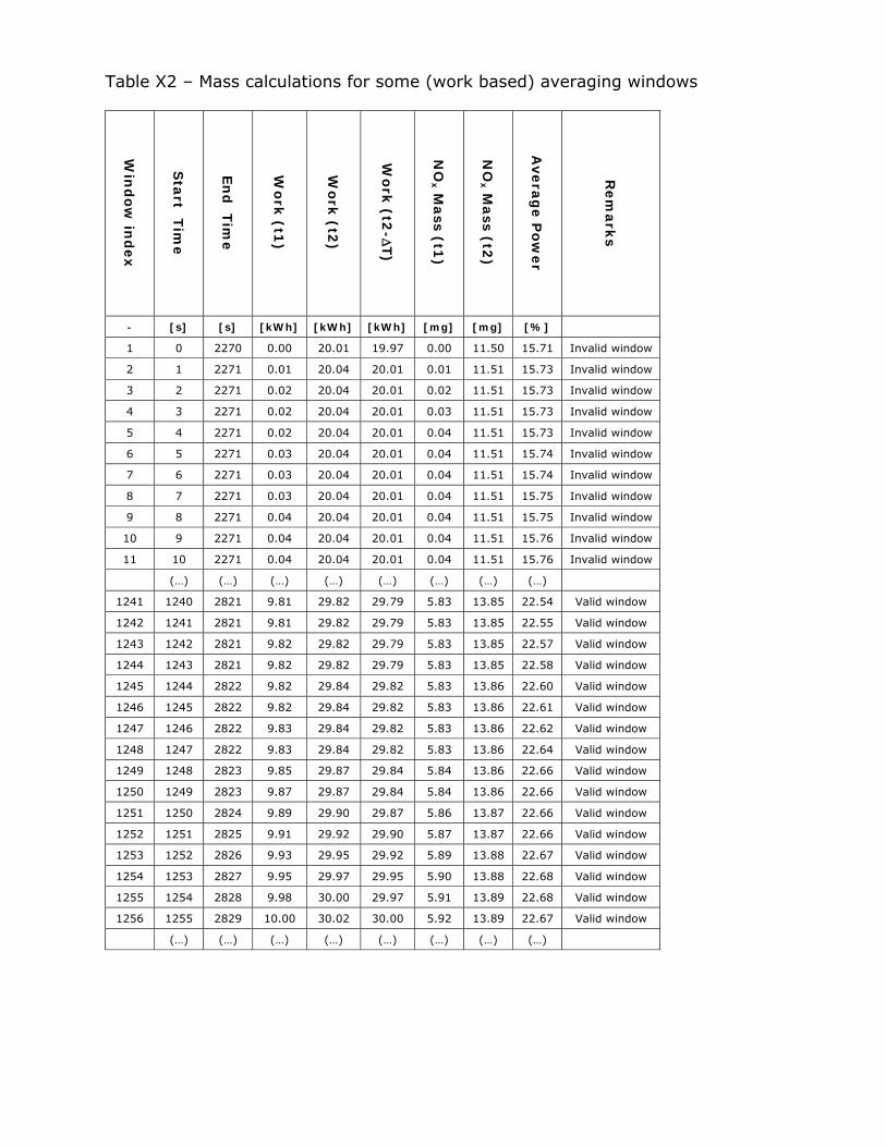
Table X2 – Mass calculations for some (work based) averaging windows

Win

do

w in

dex

Sta

rt Tim

e

En

d T

ime

Wo

rk (t1

)

Wo

rk (t2

)

Wo

rk (t2

-ΔT)

NO

x Mass (t1

)

NO

x Mass (t2

)

Avera

ge P

ow

er

Rem

ark

s

- [s] [s] [kWh] [kWh] [kWh] [mg] [mg] [%]

1 0 2270 0.00 20.01 19.97 0.00 11.50 15.71 Invalid window

2 1 2271 0.01 20.04 20.01 0.01 11.51 15.73 Invalid window

3 2 2271 0.02 20.04 20.01 0.02 11.51 15.73 Invalid window

4 3 2271 0.02 20.04 20.01 0.03 11.51 15.73 Invalid window

5 4 2271 0.02 20.04 20.01 0.04 11.51 15.73 Invalid window

6 5 2271 0.03 20.04 20.01 0.04 11.51 15.74 Invalid window

7 6 2271 0.03 20.04 20.01 0.04 11.51 15.74 Invalid window

8 7 2271 0.03 20.04 20.01 0.04 11.51 15.75 Invalid window

9 8 2271 0.04 20.04 20.01 0.04 11.51 15.75 Invalid window

10 9 2271 0.04 20.04 20.01 0.04 11.51 15.76 Invalid window

11 10 2271 0.04 20.04 20.01 0.04 11.51 15.76 Invalid window

(…) (…) (…) (…) (…) (…) (…) (…)

1241 1240 2821 9.81 29.82 29.79 5.83 13.85 22.54 Valid window

1242 1241 2821 9.81 29.82 29.79 5.83 13.85 22.55 Valid window

1243 1242 2821 9.82 29.82 29.79 5.83 13.85 22.57 Valid window

1244 1243 2821 9.82 29.82 29.79 5.83 13.85 22.58 Valid window

1245 1244 2822 9.82 29.84 29.82 5.83 13.86 22.60 Valid window

1246 1245 2822 9.82 29.84 29.82 5.83 13.86 22.61 Valid window

1247 1246 2822 9.83 29.84 29.82 5.83 13.86 22.62 Valid window

1248 1247 2822 9.83 29.84 29.82 5.83 13.86 22.64 Valid window

1249 1248 2823 9.85 29.87 29.84 5.84 13.86 22.66 Valid window

1250 1249 2823 9.87 29.87 29.84 5.84 13.86 22.66 Valid window

1251 1250 2824 9.89 29.90 29.87 5.86 13.87 22.66 Valid window

1252 1251 2825 9.91 29.92 29.90 5.87 13.87 22.66 Valid window

1253 1252 2826 9.93 29.95 29.92 5.89 13.88 22.67 Valid window

1254 1253 2827 9.95 29.97 29.95 5.90 13.88 22.68 Valid window

1255 1254 2828 9.98 30.00 29.97 5.91 13.89 22.68 Valid window

1256 1255 2829 10.00 30.02 30.00 5.92 13.89 22.67 Valid window

(…) (…) (…) (…) (…) (…) (…) (…)

European Commission EUR 24921 EN – Joint Research Centre – Institute for Energy Title: HEAVY-DUTY ENGINES CONFORMITY TESTING BASED ON PEMS Authors: Pierre Bonnel - Janek Kubelt - Alessio Provenza Luxembourg: Office for Official Publications of the European Communities 2011 – 59 pp. – 21 x 29.7 cm EUR – Scientific and Technical Research series – ISSN 1018-5593 (print), ISSN 1831-9424 (online) ISBN 978-92-79-21038-9 (print), ISBN 978-92-79-21039-6 (online) doi:10.2788/56535 Abstract The European emissions legislation requires to check the conformity of heavy-duty engines with the applicable emissions certification standards during the normal life of those engines: these are the “In Service Conformity” (ISC) requirements. It was considered impractical and expensive to adopt an in-service conformity (ISC) checking scheme for heavy-duty vehicles, which require removal of engines from vehicles to test pollutant emissions against legislative limits. Therefore, it has been proposed to develop a protocol for in-service conformity checking of heavy-duty vehicles based on the use of Portable Emission Measurement Systems (PEMS). The European Commission through DG ENTR in co-operation with DG JRC launched in January 2004 a co-operative research programme to study the feasibility of PEMS in view of their application in Europe for In-Service Conformity of heavy-duty engines. The technical and experimental activities were started in August 2004 to study the feasibility of PEMS systems and to study their potential application for on-road measurements on heavy-duty vehicles. The main objectives of the above project had been defined as follows: -To assess and validate the application and performance of portable instrumentation relative to each other, and in comparison with alternative options for ISC testing; -To define a test protocol for the use of portable instrumentation within the ISC of heavy-duty vehicles; -To assess on-road data evaluation methods such as the US ‘Not To Exceed’ (NTE) approach and possibly to develop a simplified ones; -To address the need of the European industry, authorities and test houses to go through a learning process with on-vehicle emissions testing. The main objective of the present document is to report on: a. The evaluation of the test protocol, i.e. to judge whether the mandatory data and its quality were appropriate for the final evaluation (S b. The analysis conducted to evaluate the potential of the different data evaluation (Pass/Fail) methods for ISC and in particular their ability to use on-road PEMS emissions data. The candidate methods were categorized into two families: -The "control-area / data reduction methods" (Chapter 4) that use only a part of the data, depending whether the operation points considered are part of a control area and belong to a sequence of consecutive points within this control area. The US-NTE (Not To Exceed) method - already established as an official tool in the United States - falls into this category but variations of the methods could be envisaged (with another control area for instance). -The "averaging window methods" (Chapter 4.3) that use all the operation data. The main objective of task b. was to answer the following question: “Once the data has been collected correctly, what is the most appropriate method to analyse the test data measured with PEMS and to judge whether the engine is in conformity with the applicable emissions limits?”

How to obtain EU publications Our priced publications are available from EU Bookshop (http://bookshop.europa.eu), where you can place an order with the sales agent of your choice. The Publications Office has a worldwide network of sales agents. You can obtain their contact details by sending a fax to (352) 29 29-42758.

The mission of the JRC is to provide customer-driven scientific and technical support for the conception, development, implementation and monitoring of EU policies. As aservice of the European Commission, the JRC functions as a reference centre of science and technology for the Union. Close to the policy-making process, it serves the common interest of the Member States, while being independent of specialinterests, whether private or national.

LB

-NA

-24-921-EN-N

heavy-duty engines conformity testing based on pems

Documents