Ground Penetrating Radar Theory, Data

Collection, Processing, and Interpretation:

A Guide for Archaeologists

Created by:

Lisa Dojack

April 2012

Table of Contents

Acknowledgments............................................................................................................ i Foreword ......................................................................................................................... ii

Section 1: GPR Fundamentals ........................................................................................... 1 Chapter 1. Introduction .................................................................................................. 2 Chapter 2. EM Wave Physics ........................................................................................ 4 Chapter 3. Subsurface Materials .................................................................................... 9 Chapter 4. Data Collection Parameters ........................................................................ 11 Chapter 5. Data Collected ............................................................................................ 15 Chapter 6. Signal Types............................................................................................... 18

Section 2: Data Editing and Processing ........................................................................... 19 Chapter 7. Introduction to GPR Software Programs ................................................... 20 Chapter 8. Basic Data Editing Procedures................................................................... 25 Chapter 9. Gains........................................................................................................... 31 Chapter 10. Time Filters .............................................................................................. 37 Chapter 11. Spatial Filters............................................................................................ 43 Chapter 12. 2D Filters.................................................................................................. 48 Chapter 13. Attributes.................................................................................................. 51 Chapter 14. Operations ................................................................................................ 54 Chapter 15. Data Processing Steps and Recommendations......................................... 57

Section 3: Data Interpretation .......................................................................................... 62 Chapter 16. Uncertainty and Limitations..................................................................... 63 Chapter 17. Signals of Burials and Tombs .................................................................. 67 Chapter 18. Signals of Architectural Features ............................................................. 70 Chapter 19. Conclusions and Future Directions .......................................................... 74

References Cited ............................................................................................................... 76

i

Acknowledgments

This guide grew from a term paper originally written in Dr. Andrew Martindale’s ANTH 545B Graduate Research Seminar, and it would not have been possible without the guidance and support of both Andrew and my fellow student in that class, Steve Daniel. The discussions that took place in our class were incredibly thought-provoking, and helped me to piece together my ideas on GPR in archaeology, some of which are presented here. I would like to thank Andrew for his insightful comments on and editorial assistance to preceding drafts that significantly improved the final version of this guide.

ii

Foreword

“Much of the literature available to GPR users is either manufacturers manuals (which are not directed at archaeologists or archaeological contexts), advanced analyses of detailed data sets (which assume an advanced level of understanding), or comprehensive and complex overviews (which are the best place to start). Any archaeologist considering the use of GPR equipment or the analysis of GPR data faces a steep learning curve. Conyers’ (2004) guide remains the standard and indispensable reference text for archaeologists. However, there exists a gap between the academic literature, including Conyers, and the manufacturers manuals – a gap that this guide and its companion publication (Daniel, forthcoming) – seek to fill. The ambition of this guide is to provide a concise summary of the steps and options available to the archaeologist when collecting and processing GPR data – what they mean and what they do to data. This guide seeks to summarize and explain the various options available.” – Dr. Andrew Martindale, UBC (2012) This guide was originally written as a term project for ANTH 545, a Graduate Research Seminar directed by Dr. Andrew Martindale at the University of British Columbia (UBC). Along with the purpose of expanding our general knowledge on the use of ground penetrating radar in archaeology, Steve Daniel (the other student in the class) and I were charged with producing a pair of guides or manuals about the use of the Laboratory of Archaeology (LOA) ground penetrating radar equipment. These were initially intended as teaching tools for future generations of GPR students in the department, but following further reading and extensive revisions in the year following the course, it became clear that this guide could be of interest to a larger audience. The target audience of this paper is a wide range of individuals in the archaeological community, who are understood to have varying degrees of knowledge regarding the use of GPR and the physics behind the equipment. As such, this paper does not provide an in-depth discussion of GPR or EM theory, but rather a quick introduction to those concepts and tools that are most likely to be utilized by the archaeologist in the field. This paper has been divided into three main sections. Section 1 (GPR Fundamentals) focuses on the principles of GPR: how electromagnetic radar waves move through the ground, what happens when they encounter subsurface features, and how they are imaged in GPR software programs. Section 2 (Data Editing and Processing) focuses specifically on what happens to the data after it has been collected in the field and returned to the lab, where it undergoes a variety of processes to transform it into two- and three-dimensional images of the subsurface. Section 3 (Data Interpretation) focuses on how we read these computer-generated images, and provides descriptions of the various signal types that can be produced from common archaeological features. This guide does not include information on equipment operations or data collection protocols. For more information on these subjects, the reader is directed to a companion piece by Daniel (forthcoming), which details the data collection protocols utilized by the University of British Columbia’s Laboratory of Archaeology (UBC – LOA).

iii

This is a review paper only, and does not represent an original contribution to GPR theory, data processing, analysis or interpretation. It should not be taken as a comprehensive collection and review of all GPR surveys undertaken in archaeological contexts. GPR in archaeology is a rapidly-changing and advancing field; the information provided herein is current to 2011. Note that while many of the issues discussed in this paper are relevant to all GPR users, the focus is on equipment and software manufactured by Sensors & Software. Individuals using GSSI, MALÅ, or another GPR supplier should refer to the user manuals provided by their supplier. Individuals using Sensors & Software equipment are strongly encouraged to refer to the user manuals provided by Sensors & Software. For the sake of consistency, all images presented in Section 2 are from the same profile (X Line 14 from the 2010 Test Survey) or slice (0.35-0.40 m from the 2010 Test Survey). Unprocessed or minimally processed images are provided for comparative purposes. Note that processing parameters in the processed images provided have in many cases been exaggerated to show the effect of a given processing step.

1

Section 1: GPR Fundamentals

2

Chapter 1. Introduction What is GPR? Ground penetrating radar (GPR) is one of a number of remote sensing geophysical methods utilized by archaeologists to study subsurface archaeological and geological deposits, alongside such methods as magnetometry, electrical resistivity, and electromagnetic conductivity. GPR operates in the same manner as navigational radar systems, in that it sends pulses of electromagnetic (EM) ‘radar’ waves into the ground in order to identify the shapes, sizes, and locations of subsurface features. When the transmitted EM wave encounter changes in subsurface materials, the properties of the wave are altered, and part of the wave is reflected back to the surface, where data on its amplitude, wavelength, and two-way travel time are collected for analysis. The data are collected in traces, each of which displays the total waveform of all waves collected at one surface location. When arranged in their relative positions, series of traces can produce a number of different types of images showing variations in subsurface properties in the vertical and horizontal dimensions (Annan 2009:17; Conyers 2004:11-12, 23-26; 2009:246-247; Leckebusch 2003:214). Two factors influence the success of a GPR survey: the data collection parameters utilized, which control the properties of the propagated EM wave and the ways in which its reflections are recollected at the surface; and the properties of the deposits through which the EM wave is propagated. Any changes in the physical or chemical properties of subsurface deposits (e.g., water content, compaction, presence of conductive materials such as metals, soluble salts, and some clays) can affect the properties of the EM wave in the ground, such as its velocity, amplitude, and wavelength (Annan 2009:6-8; Cassidy 2009b; Conyers 2004:45-55; Leckebusch 2003:214-215). GPR provides the best results in archaeological contexts where the target features are large, near the surface, and strongly contrasting with a homogenous surrounding matrix. Examples of this context include stone architectural features in sand matrices, such as those encountered in the Mediterranean region and the American Southwest. Benefits of GPR GPR has become an increasingly popular option for archaeological research for a number of reasons. These can be narrowed down to four key benefits: its non-destructive nature; its ability to maximize research efficiency and minimize cost; its ability to cover large areas quickly; and its high-quality three-dimensional data. As it is a remote sensing method, GPR is entirely non-invasive and non-destructive, in contrast to ‘traditional’ archaeological excavation methods, which are inherently destructive. The ability to conduct archaeological research while protecting and preserving archaeological sites (and at the very least minimizing site impacts) is becoming increasingly important, in particular where culturally sensitive features (such as human burials) are concerned. Indeed, GPR has the potential to identify these culturally-sensitive areas, and thereby ensure that they are not disturbed (Conyers 2004:1-2; 2009:245; Kvamme 2003:436; Whittaker and Storey 2008:474). GPR also has the potential to increase research efficiency. In comparison to ‘traditional’ archaeological excavation methods, GPR surveys are conducted quickly and at a relatively low cost. When used as a prospection method, GPR can aid in identifying

3

areas of high potential for future excavation (or conversely, identify areas of low potential which should be avoided), thereby maximizing relevant data collection while minimizing time and cost, in addition to site impact (Conyers 2004:1-2; 2009:245; Kvamme 2003:436; Whittaker and Storey 2008:474). Because it is such a highly-efficient research method, GPR can also be used to cover larger areas than archaeological excavations (GPR surveys can often cover several hundred square meters or more in a single day). When conducted alongside archaeological excavations, GPR can help to place excavation data into a broader site and environmental context by interpolating between excavated areas. This makes GPR particularly suitable for addressing archaeological questions at a site level and at a regional level, for example, those regarding issues of space, place, and changes in social organization over time (Conyers 2004:2; 2010; 2011; Conyers and Leckebusch 2010; Kvamme 2003:436; Thompson et al. 2011). Finally, GPR produces high-resolution three-dimensional data suitable for addressing anthropological questions (Conyers 2004:11; Leckebusch 2003:213). Leucci and Negri (2006:502) go so far as to suggest that the resolution capability of GPR is “by far greater than that obtained by other geophysical methods.” This high-resolution three-dimensional data can be easily integrated with data collected by other geophysical methods, archaeological excavation, and surface survey maps in geographic information systems (Conyers 2004:168; Leckebusch and Peikert 2001:37).

4

Chapter 2. EM Wave Physics What follows is a brief overview of how EM waves can move through the ground. For a more in-depth discussion of EM theory as it pertains to GPR, the reader can refer to Annan (2009:5-33). With advances in GPR technology and equipment, it is possible (but not advisable) for users without comprehensive knowledge of the principles of EM theory to conduct preliminary data collection; however, even basic GPR analysis requires some familiarity with this subject (cf. Conyers 2011). Cone Transmission and Centre Frequency In understanding how the EM waves propagated by GPR antenna move through the ground, it is first important to understand how these waves are propagated. The first point to note is that EM waves are emitted in a cone (the ‘cone of transmission’), which spreads out with increasing depth below the surface (Conyers 2004:66; 2009:247; Leckebusch 2003:215). The dimensions of the cone are determined by the subsurface conditions encountered and by the frequency of the energy being transmitted into the ground, with higher frequency energy resulting in narrower cones of transmission (Conyers 2004:66; Leckebusch 2003:215). The second point of note is that the energy transmitted is not limited to the centre frequency of the antenna being used. GPR transmits energy in broad band, generally with a two octave bandwidth, meaning that a range of frequencies between one half and two times the centre frequency of the antenna will be emitted (for example, a typical 500 MHz transmitter produces frequencies from about 250-1000 MHz) (Conyers 2004:39; Grealy 2006:142). For more information on centre frequency and bandwidth, see Annan (2009:19). Reflection When EM waves travelling through the subsurface encounter a buried discontinuity separating materials of different physical and chemical properties, part of the wave is reflected off the boundary and back to the surface (Conyers 2004:25, 45; Conyers 2009:247). These subsurface discontinuities may be the interfaces between archaeological features and the surrounding matrix, void spaces, or buried stratigraphic boundaries and discontinuities (Conyers 2004:25; 2009:247). The proportion and direction of the reflected EM wave are dependent upon the properties and shape of the deposit off which they are reflected. On a smooth, planar surface, the angle at which the wave will be reflected can be predicted based on the law of reflection, which states that the angle of incidence will equal the angle of reflection (with respect to the perpendicular and in the same plane):

ri θθ = where θi is the angle of incidence and θr is the angle of reflection. As the EM wave moves deeper beneath the surface, its signal weakens, and less is available for reflection (Conyers 2004:49; 2009:247). The strength of the reflected wave is also dependent upon the physical and chemical properties of the two materials from whose interface it is being reflected (Leckebusch 2003:214).

5

Refraction The part of the EM wave that is not reflected at subsurface discontinuities changes velocity, and in doing so is refracted or bent at the interface, resulting in a change in the direction of the wave through the ground (Conyers 2004:25, 45). The angle at which the wave will be refracted can be predicted based on Snell’s Law of Refraction:

1

2

2

1

2

1

sinsin

n

n

v

v==

θ

θ

where θ is the angle of incidence (1) or refraction (2), v is the velocity, and n is the index of refraction. Refraction explains why the cone of transmission becomes increasingly narrow with depth (Conyers 2004:66; 2009:247; Leckebusch 2003:215). In addition, Snell’s Law can provide the critical angle beyond which EM waves cannot propagate between two different materials: this occurs when v1 is greater than v2 (Annan 2009:13). For more detail on reflection and refraction, see Annan (2009:13-14). Diffraction In physics, ‘diffraction’ refers to the bending of waves around objects, or the spreading of waves as they pass through narrow openings. Diffraction may occur around steeply sloping or vertical surfaces, resulting in increased radar wave travel time and therefore distortion of the depth, location, size, and geometry of the object (Cassidy 2009a:165; Conyers 2004:128). In the case where velocities change along the vertical axis of these objects, a phenomena known as pull-up and pull-down occur; these terms describe the underestimation or overestimation of the depth of the lower boundary of the feature in question (Leckebusch 2007:142-143). In GPR theory, diffraction is more commonly applied to the phenomenon that produces point source hyperbolas. The hyperbolic image produced from point source reflectors is due to the fact that GPR energy is emitted in a cone, which radiates outwards with depth. As such, energy is reflected from objects that are not directly below the antenna; the reflection, however, is recorded as being directly below the antenna, and at a greater depth due to the oblique transmission of the wave. Only the apex of the hyperbola denotes the actual location of the point source (Cassidy 2009a:165; Conyers 2004:56-58; Leckebusch 2003:215). Scatter and Focusing The term ‘scatter’ is used to refer to the phenomenon of waves being reflected away from the range of the receiving antenna; such waves are not collected by the GPR. This phenomenon occurs on surfaces sloping away from the antenna, on convex up surfaces, in deep narrow concave features, and in near vertical features (Conyers 2004:67, 73-74; 2009:348). Other generally resolvable features located near deposits that produce a high degree of scatter may also be obscured by this phenomenon (Conyers 2004:73). Conyers (2009:248) suggests collecting data in closely spaced perpendicular transects to reduce the effects of scatter. Sinuous data collection (alternating data collection direction along one dimension) may also allow sloping surfaces to be imaged. For more information on signal scattering, see Annan (2009:16-17). The opposite of scattering is focusing, which occurs when waves are reflected off surfaces sloping towards the antenna or within shallow wide concave up features. This

6

results in high-amplitude waves being reflected back to the receiving antenna, and in some cases, multiple reflections within these features, which may distort depth, location, size, or geometry (Conyers 2004:73-74). Dispersion, Dissipation, and Attenuation As EM waves propagate to greater depths, they become increasingly dispersed due to the electrical conductivity of subsurface materials, until such point as they are fully dissipated or attenuated, and no energy is reflected back to the surface (Conyers 2004:49, 91; Leckebusch 2003:214). The rate of attenuation or dissipation is relative to the frequency of the transmitted wave and the properties of the subsurface materials it encounters. Higher frequency waves are more readily attenuated, and therefore have shallower penetration depths (Conyers 2004:91; Leckebusch 2003:214). It is important to note that waves experience dispersion, dissipation, and attenuation in both vertical directions – reflected waves may be attenuated on the way back to the receiving antenna, and will therefore not be collected (Conyers 2009:247). Multiples, Ringing, and Reverberation Multiples or ‘ring-down’ occur when EM waves encounter highly-reflective or impermeable objects (such as metals), and are due to multiple reflections between the metal object and the surface. The result is multiple stacked reflections being imaged below the metal object (Conyers 2004:54, 79). Ringing refers to system noise produced from the antennas, and is visible in reflection profiles as horizontal banding, usually in the upper portion of the profile (Conyers 2004:123). Reverberation, like ring-down, produces multiples in reflection profiles, but is a result of system noise produced from ‘ringing antennae’ which reverberate when spaced too closely (Conyers 2004:127-128). Background Noise and Clutter Not all waveforms collected are due to subsurface reflections. Especially in the case of unshielded antenna, reflections may be collected from nearby above ground objects, such as buildings and trees; these generally produce high amplitude linear reflections (Conyers 2004:77). Background noise may also be generated by other nearby sources of EM waves, including televisions, cell phones, and radio transmission antennas; GPR survey can be especially compromised by background signals in areas near airports, military bases, or busy roads (Conyers 2004:71-73). The GPR antennae also contribute to background noise, in that they produce an EM field that obscures signals within 1.5 wavelengths of the antenna (Conyers 2004:36, 77; 2009:248). Background noise produced from subsurface reflections is termed clutter, and refers to point targets and small discontinuities that reflect energy and obscure the signals of other more important reflected waves. Clutter can be minimized by selecting antennas of lower frequency, which will not resolve small objects (Conyers 2004:67; 2009:249).

7

Ground Coupling and Antenna Tilt Ground coupling refers to the degree to which the GPR antenna are in contact with the ground surface when transmitting and receiving EM waves. When the antenna are pulled over the ground surface, any sudden changes in height above the surface (due to roots, rocks, and uneven surfaces) can result in coupling loss, which will affect penetration depth and reflection amplitudes (Conyers 2004:68-71). Ground coupling may be complicated on topographically complex surfaces, which themselves introduce added complications to accurately imaging subsurface features. When GPR survey is conducted on sloping surfaces with the antenna on a tilt, energy is transmitted in various non-vertical directions and reflected from objects not located directly beneath the antenna; however, the computer records the reflection as being reflected from locations directly below the antenna. This results in distortion of the depth, location, size, and geometry of the object (Conyers 2004:123; Goodman et al 2006:157). Goodman et al. (2006:158) have devised a method to correct for antenna tilt by calculating the angle of the antenna based on static correction of the ground surface, then shifting reflection traces to their correct positions. Controlled Experiments An understanding of how EM waves move beneath the ground surface is aided by controlled experimental studies, the value of which cannot be overstated. One such study conducted by Leckebusch and Peikert (2001) involved taking a number of measurements in a sandbox to examine the resolution of GPR data and the effects of antenna orientation. Control measurements were taken in the sand box prior to the introduction of any subsurface structures; the data generated from this control survey was taken as the background signal, and was removed from all other data sets produced (Leckebusch and Peikert 2001:30-31). The first experiment involved imaging a single concrete block (22 x 15 cm wide, 95 cm long) (Leckebusch and Peikert 2001:31). Both the upper and lower boundaries of the block were imaged perfectly; the vertical sides produced no signals (Leckebusch and Peikert 2001:32). It was also found that signal strength decreased significantly beneath the block, and imaging of objects below a strongly reflecting object was difficult (Leckebusch and Peikert 2001:36). The second experiment involved imaging two concrete blocks buried one on top of the other, with a gap of 10 cm (Leckebusch and Peikert 2001:31). The upper block was imaged perfectly, as in the first experiment; however, only the upper boundary of the lower block was potentially visible in the profile, and was instead attributed to the presence of multiples, which obscured the lower block. Amplitude slices showed the blocks being surrounded by a semi-circular reflection; this was attributed to gravitational sand grain size separation which occurred when the blocks were covered over with sand (Leckebusch and Peikert 2001:32). The third experiment involved imaging two round stones placed directly on top of one another (Leckebusch and Peikert 2001:31). It was found that the two stones could not be distinguished, and the image size was distorted, with the stones appearing a few centimetres larger than in reality (Leckebusch and Peikert 2001:33). The fourth experiment examined the affects of antenna orientation on object visibility by conducting surveys over a block of concrete, each diverging 10° from the

8

primary axis (0°), defined as perpendicular to the long-axis of the block (90° represents readings parallel to the long-axis of the block). Results showed that upon passing from 50° to 60°, the concrete block could not be imaged, thereby exhibiting that detection is dependant upon relative orientations of the antenna and structure to be imaged (Leckebusch and Peikert 2001:34).

9

Chapter 3. Subsurface Materials The initial success of GPR survey is primarily dependent upon two factors: the data acquisition parameters (which control the waveform transmitted into the ground and the ways in which it is collected back at the surface), and the characteristics of the materials through which the EM waves are propagated (Conyers 2004:50; Orlando 2007:213). A number of subsurface physical and chemical properties influence the ability of radar waves to be propagated into and reflected within the ground, including electrical and magnetic properties, water content, lithology, density, and porosity (Cassidy 2009b; Conyers 2004:25, 55, 247). With advances in GPR technology and equipment, it is possible (but not advisable) for users without comprehensive knowledge of the effects of certain subsurface materials on the EM waves being propagated and collected to conduct preliminary data collection; however, even basic GPR analysis requires some familiarity with this subject (cf. Conyers 2011). Electrical Conductivity (σ) describes the ability of a material to conduct away the electric portion of the EM wave. Materials which are more electrically conductive will more readily conduct away the electric part of the EM wave, thereby dissipating or attenuating the wave and resulting in shallow subsurface imaging; conversely, materials with a low electrical conductivity will allow greater depth of EM wave permeation (Annan 2009:6-7; Conyers 2004:50). For information on electrical conductivity values of common materials, refer to Cassidy (2009b:46) or Leckebusch (2003:215). Magnetic Permeability (µ) describes the ability of a material to become magnetized in the presence of an EM field. Materials that are more magnetically permeable will more readily interfere with the magnetic part of the EM wave, thereby attenuating the wave and resulting in shallow subsurface imaging (Annan 2009:6-7; Conyers 2004:53-54). For information on magnetic permeability values of common materials, refer to Leckebusch (2003:215). Dielectric Permittivity (ε) describes the ability of a material to store and transmit an electric charge induced by an EM field (Annan 2009:6-7). The dielectric permittivity of a material is also described by its Relative Dielectric Permittivity (RDP; κ or εr), which is defined by the equation:

0ε

εκ =

where κ is the RDP, ε is the dielectric permittivity, and ε0 is the permittivity of a vacuum (8.89×10-12 F/m) (Annan 2009:7). RDP can be used to estimate radar wave velocity and wavelength (or amplitude), with higher RDP materials having lower wave velocities and lower amplitudes. RDP can therefore be taken as a general measure of the depth to which radar waves will penetrate the ground (Cassidy 2009b:45-54; Conyers 2004:45-49, 59; Leckebusch 2003:214). RDP is calculated from the equation:

10

2

=

v

crε

where εr is the RDP, c is the speed of light (0.2998 m/ns), and v is the velocity of waves through the material (in m/ns) (Conyers 2004:48; Leckebusch 2003:214). It is important to note that RDP (and therefore wave velocity) varies with depth, as different materials are encountered (Leckebusch 2003:214). For information on RDP (εr) values and velocities of common materials, refer to Cassidy (2009b:46), Conyers (2004:47), or Leckebusch (2003:215). Specific Materials Conyers (2004:100) identifies water content as the “single most significant variable” in affecting RDP and therefore wave velocity and reflection, a sentiment echoed by Annan (2009:8) and Cassidy (2009b:45). The fact that water content often increases with depth is one of the factors affecting the attenuation of radar waves with increasing depth (Conyers 2004:101). Salt water, or the presence of any soluble salts or electrolytes in the soil, is particularly detrimental to GPR survey, as these materials have a high electrical conductivity due to their ability to create free ions when dissolved in water (Conyers 2004:37, 50-53). This makes them essentially impermeable reflectors of the EM signal. Other materials with similar properties resulting in high conductivity include sulfates, carbonate minerals, and charged elemental species of minerals (Conyers 2004:52). Certain clays also pose a problem in successfully conducting GPR surveys. These include three-layer swelling clays, such as montmoriollionite, smectite, and bentonite, all of which are highly conductive. The conductivity of these clays is increased further when wet. Other clays (such as two-layer kaolinites and three-layer non-swelling illites) show no such heightened conductivity (Conyers 2004:50-53). Radar waves will not penetrate metals; instead, the wave is reflected in its entirety back to the surface, and thus blocks the detection of deposits below the metal object (Conyers 2004:54). As metal is both highly electrically conductive and magnetically permeable, soils which are iron-rich or incorporate magnetite minerals or iron oxide cements will also attenuate radar waves (Conyers 2004:53-54).

11

Chapter 4. Data Collection Parameters While the RDP (as an expression of the properties of subsurface materials) cannot be controlled for in GPR surveys, there are numerous other parameters that can be varied to achieve the targeted depth and resolution. These include antenna frequency, time window, sample interval, samples per trace, step size, stacking, and transect spacing and orientation. Antenna Frequency and Depth As previously noted, the ability of EM waves to effectively penetrate the ground to a particular depth is primarily dependent upon two factors: the frequency of the waves, and the characteristics of the ground (Conyers 2004:50). As only wave frequency can be controlled for, choosing the correct antenna frequency for a GPR survey is critical. Lower frequency antennas with long wavelengths provide the deepest penetration, whereas high frequency antennas with short wavelengths are only able to image shallow features (Conyers 2004:23, 41-42, 58; Grealy 2006:142; Neubauer et al. 2002:139). Conyers (2004:60) suggests as a general rule that 400-900 MHz antenna should be used to image features within 1 m of the surface, whereas images 1-3 m below the surface are best imaged with 250-500 MHz antenna. Goodman et al. (2009:485) recommend selecting a radar frequency (and time window length) that will collect information to a depth of at least 1.5-2 times that of the target area. Antenna Frequency and Resolution Resolution of subsurface features is in part affected by antenna wavelength (which is directly related to antenna frequency), with higher frequency antenna providing higher resolution than lower frequency antenna (Conyers 2004:23, 41-42, 58, 88; Grealy 2006:142; Leckebusch 2003:215; Neubauer et al. 2002:139). The reason for this is that the shorter wavelengths of high frequency produce a narrower cone of transmission, which can focus on smaller areas and thereby resolve smaller features than the more spread out transmission cones produced by antennas with low frequencies and longer wavelengths (Conyers 2004:65-66). The centre frequency wavelength of an antenna can be calculated from the equation:

Kf

c=λ

where K is the RDP, c is the speed of light (0.2998 m/ns), and f is the centre frequency of the antenna (in MHz), and λ is the centre frequency wavelength of the antenna (in m) (Leckebusch 2003:215). Maximum resolution of horizontal features is roughly equivalent to the area of the energy footprint (or area of illumination), which varies with frequency and depth (Conyers 2004:61-63; Grealy 2006:143-144). The footprint size can be calculated from the equation:

14 ++=

K

dA

λ

where A is the long dimension of the elliptical footprint, λ is the centre frequency wavelength of the antenna (in m), d is the depth below the surface (in m), and K is the

12

average RDP from the surface to depth d (Conyers 2004:62). The maximum resolvable horizontal target is equivalent to A, the long dimension of the footprint. A ‘rule of thumb’ for determining appropriate frequency is that the smallest object that can be resolved is approximately 25% of the wavelength in the ground (Conyers 2004:59). Maximum resolution of vertical features is roughly equivalent to or larger than half the wave length (Neubauer et al. 2002:139). Vertically stacked horizontal interfaces must be separated by at least one wavelength if they are to be resolved (Conyers 2004:64). For more information on resolution, see Annan (2009:14-16). Here it is important to reiterate that GPR produces EM waves in a broadband, such that frequencies from one half to two times that of the centre frequency are present (Conyers 2004:39; Grealy 2006:142; Leckebusch 2003:215; see also Chapter 2). For example, a typical 500 MHz transmitter produces frequencies from about 250-1000 MHz. High frequency data can then be filtered out of any given data set to produce images with higher resolution, while low frequency data can be filtered out to image deeper features (see Grealy 2006:142-144). Time Window is the amount of time for which the receiving antenna will record two-way travel time data. Conyers (2004:85-87) suggests the time window be at least as long as the time it takes to resolve the maximum depth desired; for 2-3 m depth, the suggested time window is 100 ns. For a more precise measure, the suggested time window can be calculated using the equation:

=

v

dW

23.1

where W is the length of the time window (in ns), d is the maximum depth to be resolved (in m), and v is the minimum velocity of waves through the material (in m/ns). The time window is increased by 30% to allow for uncertainty in measurements of d and v (Sensors & Software 1999a:8). Longer time windows require larger numbers of samples per trace to adequately resolve the recorded waveform (Conyers 2004:87-88). Sampling Interval refers to the time between points collected for each recorded waveform. The sampling interval should not exceed half the period of the highest frequency, taken to be 1.5 times the centre frequency of the antenna; it can be calculated using the equation:

ft

61000

=

where t is the sampling interval (in ns) and f is the centre frequency of the antenna (in MHz) (Sensors & Software 1999a:9). Samples per Trace refers to the number of incremental pulses (samples) needed to construct a single reflection trace from the 25,000-50,000 (or more) radar pulses transmitted per second by the GPR (Conyers 2004:28-30). This parameter influences resolution in that collecting more samples results in a higher resolution of the reflected waveform (Conyers 2004:87). Larger numbers of samples per trace require longer time windows for their collection, and higher frequency antenna require more samples per trace to adequately define the reflected waveform (Conyers 2004:87-88). The minimum number of samples collected per trace in most GPR surveys is 512; other common values

13

are 1024 and 2048 samples per trace (Conyers 2004:30, 87). The number of samples per trace varies with time window and sampling interval as described by the equation:

=

t

WS

where S is the samples per trace, W is the time window (in ns), and t is the sampling interval (in ns). Step Size is the spatial sampling interval, which defines how often a trace is collected spatially (for example, one trace every 0.02 m). The smaller the step size, the higher the resolution of the data collected. Stacking refers to the averaging of successive reflection traces to produce a composite trace; the number of stacks parameter defines the number of consecutive traces that are averaged to produce the composite trace. One of the primary benefits of stacking is that it increases data quality and resolution, as the averaging process effectively filters out noise caused by minor changes in subsurface water content, small rocks, voids, and minor changes in amplitude due to coupling differences (Conyers 2004:88-89). Higher numbers of stacks result in slower data collection. Number of stacks is commonly set at 4, 16, 32, and 64. Transect Spacing can also affect resolution of subsurface features. The effect of transect spacing on resolution is best demonstrated by a number of experiments in which line spacing was varied to assess the affect on resolution. In general, Sensors & Software (1999a:12) suggests transects should be separated by less than the long dimension of the footprint (the area covered by the cone of transmission at a given depth). Based on the Nyquist rule, Leckebusch (2003:216) recommends a standard transect spacing of 25 cm for 400-500 MHz antenna. For more information on sampling criteria and the Nyquist rule, see Annan (2009:29). One experiment by Neubauer et al. (2002:139-141) conducted surveys over 1.5 m thick stone walls using transect spacings of 0.5 m, 1.0 m, and 2.0 m. It was determined that the transect spacings of 1.0 m and 2.0 m did not adequately resolve the subsurface features, and a transect spacing of 0.5 m or less is highly recommended. Another transect spacing experiment conducted by Orlando (2007:219) found that the geometry of subsurface features was distorted when surveyed with a transect spacing of 1 m; this was attributed to the application of an interpolation algorithm to construct slices. Again, a transect spacing of 0.5 m or less is recommended. A final published example is the experimental survey conducted by Pomfret (2006:153), which imaged subsurface features using transect spacings of 25 cm and 50 cm. While the results of the survey with transect spacing 25 cm were better resolved, no additional features were identified as compared to the survey taken with transect spacing 50 cm, and hence a 50 cm transect spacing is recommended to decrease data collection time.

14

Transect Orientation is also shown to have an effect on resolution. Neubauer et al. (2002:141) conducted surveys in the x and y directions with transect spacing 0.5 m and 1.0 m. It was determined that walls were best resolved in perpendicular sections, and the best resolution overall combined data from both the x and y directions; however, it was also noted that single direction surveys with transect spacing 0.5 m had higher resolution than did composite x and y surveys with transect spacing 1.0 m. This illustrates that the utility of GPR as an investigation tool is often improved when basic site features, such as the orientation of architecture or features, is known. Another transect orientation experiment conducted by Pomfret (2006:152-153) also found that linear subsurface features were best resolved when transects were collected perpendicular to them, and that composite x and y surveys were the preferred data collection method, as they provided the greatest resolution. Experimental studies on clandestine graves by Schultz and Martin (2011:64) also come to the conclusion that composite x and y surveys are the preferred method. For another example of the effects of transect orientation and spacing on imaging results, see Orlando (2007).

15

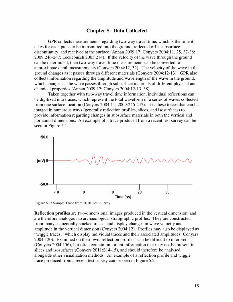
Chapter 5. Data Collected GPR collects measurements regarding two-way travel time, which is the time it takes for each pulse to be transmitted into the ground, reflected off a subsurface discontinuity, and received at the surface (Annan 2009:17; Conyers 2004:11, 25, 37-38; 2009:246-247; Leckebusch 2003:214). If the velocity of the wave through the ground can be determined, then two-way travel time measurements can be converted to approximate depth measurements (Conyers 2004:12, 32). The velocity of the wave in the ground changes as it passes through different materials (Conyers 2004:12-13). GPR also collects information regarding the amplitude and wavelength of the wave in the ground, which changes as the wave passes through subsurface materials of different physical and chemical properties (Annan 2009:17; Conyers 2004:12-13, 38). Taken together with two-way travel time information, individual reflections can be digitized into traces, which represent the total waveform of a series of waves collected from one surface location (Conyers 2004:11; 2009:246-247). It is these traces that can be imaged in numerous ways (generally reflection profiles, slices, and isosurfaces) to provide information regarding changes in subsurface materials in both the vertical and horizontal dimensions. An example of a trace produced from a recent test survey can be seen in Figure 5.1.

Figure 5.1: Sample Trace from 2010 Test Survey Reflection profiles are two-dimensional images produced in the vertical dimension, and are therefore analogous to archaeological stratigraphic profiles. They are constructed from many sequentially stacked traces, and display changes in wave velocity and amplitude in the vertical dimension (Conyers 2004:12). Profiles may also be displayed as “wiggle traces,” which display individual traces and their associated amplitudes (Conyers 2004:120). Examined on their own, reflection profiles “can be difficult to interpret” (Conyers 2004:156), but often contain important information that may not be present in slices and isosurfaces (Conyers 2011:S14-15), and should therefore be analysed alongside other visualization methods. An example of a reflection profile and wiggle trace produced from a recent test survey can be seen in Figure 5.2.

16

Figure 5.2: Sample Reflection Profile (left) and Wiggle Trace (right) from 2010 Test Survey Slices are computer-generated two-dimensional images produced in the horizontal dimension, and are therefore analogous to archaeological spatial maps or plan views. They are used to spatially map variations in EM wave amplitude at different times or depths below the surface (Conyers 2004:148; 2006b:71; 2009:249). Slices are suggested as the optimal method for quickly imaging GPR detected spatial anomalies, in particular for large areas (Leucci and Negri 2006:503; Yalçiner et al. 2009:1684-1685). An example of a slice produced from a recent test survey can be seen in Figure 5.3. Multiple slices can also be stacked atop one another to produce useful three-dimensional images of the subsurface (Conyers 2004:148), or can be crosscut with reflection profiles to produce three-dimensional fence diagrams.

Figure 5.3: Sample Slice (left) and isosurface (right) from 2010 Test Survey

Isosurfaces are true three-dimensional images that represent interfaces of a constant amplitude value (Conyers 2004:162). Multiple isosurfaces of different amplitude value can be colour-coded and displayed simultaneously, and even exported into GIS programs (Leckebusch and Peikert 2001:37). Isosurfaces are suggested as the best method for imaging small areas in high detail (Leucci and Negri 2006:503). An example of an isosurface map produced from a recent test survey can be seen in Figure 5.3.

17

Velocity Tests The velocity of the EM wave in the ground is the basis for converting two-way travel times into approximations of depth. It can be determined through a number of field methods, all of which calculate velocity from measurements of the travel time of energy pulses along a known distance of the material to be tested (Conyers 2004:13, 105). The most common of these are common midpoint (CMP), wide-angle refraction and reflection (WARR), reflected wave method, and transillumination. CMP and WARR measure travel time of waves sent between two antennae that are moved apart at known distances. The only difference in these two methods is that in CMP both antennae are moved apart from a fixed central point, whereas in WARR one antenna in moved away from the other, which remains in fixed position (Conyers 2004:106-109; Sensors & Software 1999a:2, 14; 1999b:8-12). The reflected wave method involves burying a metal bar at known depth and recording two-way travel time over its location (Conyers 2004:102-105). Transillumination records the travel times of waves sent between two vertically oriented antennae facing each other in excavation units. The primary benefit of the transillumination method is the ability to collect velocity measures through different stratigraphic layers (Conyers 2004:109-112). Sensors & Software (1999a:14) suggest CMP is the preferred method, noting that the “reflected signal is more likely to come from a fixed spatial location.” Conyers (2004:100-101) suggests conducting multiple velocity tests across a site and over a number of days to account for changes in velocity over the spatial extents of the site as well as the temporal extents of the survey period. Velocities attained from velocity tests can also be affirmed by computer hyperbola-fitting, which calculates velocity based on the dimensions of point source hyperbola reflections (Cassidy 2009a:166; Conyers 2004:115-116).

18

Chapter 6. Signal Types The effect of subsurface materials on the propagating EM wave varies depending on the size, orientation, and chemical and physical properties of subsurface archaeological features and geological deposits. The result is a wide range of signal patterns, all of which fall under one of two basic categories: planar reflections, produced at transitions between deposits and/or features; and point source reflections, produced by discrete point targets. In addition, signals can be distinguished by variations in amplitude, as dictated by changes in subsurface materials and their effects on the amplitude of the EM wave. Planar Reflections are reflections that appear as horizontal or sub-horizontal lines in reflection profiles. They are generated from any lineal boundary between materials, such as buried stratigraphic and soil horizons, the water table, and horizontal archaeological features, such as house floors (Conyers 2004:55-56; 2009:248). These require only one distinct reflection to be resolved in reflection profiles (Conyers 2009:248). Planar reflections can be used to approximate the shape, depth, size, and orientation of subsurface boundaries and discontinuities. Point Source Reflections are reflections which often appear as hyperbolas in reflection profiles. They are commonly generated from distinct, spatially-restricted, non-planar features (‘point targets’), such as rocks, metal objects, walls, tunnels, voids, and pipes crossed at right angles (Conyers 2004:54, 56; 2009:248). For these three-dimensional objects to be resolved, reflections must be received from at least two of the object’s surfaces (Conyers 2009:248). Hyperbolas are a form of point source reflection, and are due to the fact that GPR energy is emitted in a cone, which radiates outwards with depth. The hyperbolic image produced from point source reflectors is due to the fact that GPR energy is emitted in a cone, which radiates outwards with depth. As such, energy is reflected from objects that are not directly below the antenna; the reflection, however, is recorded as being directly below the antenna, and at a greater depth due to the oblique transmission of the wave. Only the apex of the hyperbola denotes the actual location of the point source (Cassidy 2009a:165; Conyers 2004:56-58; Leckebusch 2003:215). Amplitude Changes are due to the variations in subsurface material properties. High amplitude reflections are generated at boundaries between materials of highly contrasting physical and chemical properties, and thus RDP values. In contrast, low amplitude values reflect materials of similar properties or uniform matrixes (Conyers 2004:49, 149, 249; Neubauer et al. 2002:142). Metal objects produce very distinct reflections, which are characterised by multiple stacked high-amplitude reflectors, referred to as multiples (Conyers 2004:54).

19

Section 2: Data Editing and Processing

20

Chapter 7. Introduction to GPR Software Programs EKKO View EKKO View is a proprietary software package from Sensors & Software for basic processing of GPR data collected using their GPR arrays. It is the most basic program for viewing and processing reflection profiles (so basic in fact that there appears to be no user manual). Options in the File menu include Copy Image to Clipboard and Save As, to export the image to other programs. The export image type can be selected under Preferences (jpeg, bitmap, or enhanced meta file). The Axes and Scale menus are used to change position axis, time axis, depth axis, and grid lines parameters, including axis scaling, label intervals, titles, grid line orientation and visibility. The Image menu gives display options for the image, including the image type (colour scale or wiggle trace), the colour table, and interpolation. The Options menu is used to display the header file, change the plot title and trace comments display options, estimate velocity through hyperbola curve fitting, and zoom in and out. The Processing menu provides access to basic processing steps, including dewow and gains (AGC, SEC, Auto, Constant, or none). EKKO View Deluxe EKKO View Deluxe is the most advanced program for processing GPR reflection profile data supplied by Sensors & Software. It can be used before or after GFP Edit (but note the two programs use a number of the same editing processes which should not be repeated in the second program), but should be used prior to EKKO Mapper and Voxler. If data has been processed in EKKO View Deluxe and is later imported into EKKO Mapper, DME processing (dewow, migration, and envelope) and background subtraction should be turned OFF in EKKO Mapper. Amplitude equalization should also be turned off if gains have been applied (Sensors & Software 2007a:19, 51, 55). Projects are created in EKKO View Deluxe, and are composed of all the GPR data (.HD and .DT1 files) in a single folder. New projects can be created under File � New Project by selecting the desired folder under ‘Input Directory.’ Existing projects can be opened under File � Open Project. See Sensors & Software (2003:5-6, 17) for more detail. Edit/Process Mode is used to edit and/or process GPR data. Unless this button is selected at the top of the screen upon creating or opening a project, data is displayed in original data mode only, and cannot be edited, processed, or deleted. Upon selecting Edit/Process, all highlighted/selected data files are copied and saved in a new or existing subfolder in the original folder. Note that it is only these copies that are changed, not the original data files. Edited and processed data files can be replaced with the original files under Edit � Reset All Files, or by right-clicking on the highlighted/selected file(s) and selecting ‘Reset.’

21

To edit/process data, first select the data file(s) of interest. Editing is applied under the ‘Data Editing’ menu (see Basic Data Editing for more detail). Editing can also be accomplished by right-clicking on the data file or adjacent column and selecting the desired process from the menu. Processing is accomplished by adding processes from the ‘Insert Process’ menu (see Chapters 9-14 for more detail) to the processing window at the bottom of the screen, then selecting the ‘Apply’ button. The order in which processes are applied can be changed by highlighting the process, then moving it up or down the list with the arrow buttons to the left. The properties of each process can be changed by double-clicking or right-clicking on the process and selecting ‘properties’ from the menu. Processes can be deleted from the list using the delete key or right-clicking and selecting ‘delete’ from the menu. See Sensors & Software (2003:7-8, 10-13, 19-20) for more detail. View options in EKKO View Deluxe include sections (reflection profiles), individual traces, processing history, trace headers and comments, and average time-amplitude and amplitude spectrum plots. These can be accessed in the View menu, or by right-clicking on individual data files and selecting the View menu. All sections (reflection profiles) are displayed in EKKO View. See Sensors & Software (2003:21-27) for more detail. GFP Edit GFP Edit is a program from Sensors & Software for creating and editing GFP files, which contain relational information about GPR data lines. It can be used before or after EKKO View Deluxe (but note the two programs use a number of the same editing processes which should not be repeated in the second program), but must be used prior to EKKO Mapper and Voxler. GFP Files are created under File � Create New GFP for Grid Lines. GPR data lines can be added to the file using Edit � Import Line(s), then selecting the required files (note the GFP file must be in the same folder as these files or a subfolder containing these files). The Import Line Parameters window will appear upon importing new GPR data lines. This window provides the most basic data editing options, including line type, direction, spacing, and offset. See Sensors & Software (2007b:4, 12, 23-32) for more detail. Editing GFP files can be done by selecting the GPR data line(s) and accessing the Editing window under Edit � Edit GFP File, by pressing F5 on the keyboard, or by right-clicking on the data line(s) in the grid table. The Name tab in the Editing window allows the name of individual lines to be changed. The Orientation tab gives options for changing the line type (x or y), orientation (forward or reverse), and ordering (flip x or y). The Position tab is used to move lines to a new position. The Length tab is used to change the line length by recalculating step size; note that this operation does not remove data, but acts as a simple ‘rubber-banding’ operation. The length of a line can also be edited by manually changing the step size under the Step Size tab. The Line Spacing tab

22

is used to define the distance between GPR data lines. See Sensors & Software (2007b:13-21) for more detail. EKKO Mapper EKKO Mapper from Sensors & Software is used to create slices and view and process slices and sections (reflection profiles). It is best used after data has been processed in EKKO View Deluxe, but can be used on its own if only basic processing steps are desired. If data has been processed in EKKO View Deluxe and later imported into EKKO Mapper, DME processing (dewow, migration, and envelope) and background subtraction should be turned OFF in EKKO Mapper. Amplitude equalization should also be turned off if gains have been applied (Sensors & Software 2007a:51, 55). The Data Processing Window will appear upon opening a GFP file for the first time. It can also be accessed under Tools � Data Processing. Processing options include data position limits, velocity, background subtraction, slice processing, DME (dewow, migration, and envelope) processing, and amplitude equalization (see time filters, spatial filters, 2D filters, and attributes for more detail). Data position limits options include outer (longest lines define grid size), inner (shorted lines define grid size), clipped (boundary x and y lines define grid size), and user defined. Slice processing involves selecting the thickness of the slice, what percentage overlaps with the previous slice, the depth and interpolation limits, and slice resolution (max, high, medium, low, or user-defined). See Sensors & Software (2007a:49-62) for more detail. Hyperbola Velocity Estimate is used to estimate the signal velocity by curve fitting. It can be accessed in the Data Processing window or under Tool � Hyperbola Velocity Calibration. This tool should only be used for hyperbolas which are created by objects known to have been crossed at right angles. To estimate velocity, click on the apex of a hyperbola to drop the curve on this location, then drag the tails of the curve to fit it to the shape of the hyperbola. To estimate the velocity when there is an object of known depth in the profile, position the apex on the top surface of the known object and adjust the velocity until the depth displayed at the bottom of the screen is equal to that of the object. See Sensors & Software (2007a:53, 63-65) for more detail. The Plan View Window & Legend displays GPR slices and associated information, including the file name, slice range, lines, velocity, frequency, settings (sensitivity, contrast, background subtraction, dewow, migration, envelope, amplitude equalization, interpolation limit, resolution, and colour palette), collection date, and analyzed date. Slices are most efficiently navigated using the Page Up and Page Down keys on the keyboard, the mouse wheel, or clicking on the desired depth on the reflection profile. The image can be zoomed and panned by selecting these options under the View menu or on the toolbar at the top of the page. Collected lines, scale grid, and plan legend can be toggled on and off using buttons on the toolbar at the top of the page or under the View menu. See Sensors & Software (2007a:4-6, 11-12, 40-43, 47) for more detail.

23

The Cross-Section Window & Legend displays GPR sections (reflection profiles) and associated information, including the line name, velocity, sensitivity, contrast, background subtraction, dewow, migration, envelope, gain, and colour palette. Sections are most efficiently navigated using the up and down arrow keys on the keyboard, or clicking on the desired line on the plan view. The image can be zoomed and panned by selecting these options under the View menu or on the toolbar at the top of the page. Scale grid and section legend can be toggled on and off using buttons on the toolbar at the top of the page or under the View menu. See Sensors & Software (2007a:4, 6-7, 12, 40-43, 47-48) for more detail. The Settings Window can be opened under the View menu, and is used to select slice and section viewing options. Slice settings include lines, colour palette, sensitivity, contrast, and cursor/line/scale colours. Cross-section settings include processing, colour palette, sensitivity, contrast, cursor and scale colour, depth limit, and gain. Contrast controls the percentage of the image area which is displayed at the extremes of the colour palette, and is used to increase the visibility of weak signals. Sensitivity controls the sensitivity of the image to signal variations by narrowing the colour palette around the zero signal level, and is used to increase the visibility of weak signals. See Sensors & Software (2007a:25-39) for more detail. Export Image can be accessed under the View menu, and is used to copy the image from the selected window to a clipboard, save the image as a BMP, JPG, PNG, TIFF, or GIF graphic file, or print the image. See Sensors & Software (2007a:23-24) for more detail. Export 3D Data is an option whereby the GFP file displayed in EKKO Mapper is exported and converted to an HDF or CSV file, which can then be imported into Voxler for three-dimensional visualization. This option can be accessed under File � Export 3D Data to File. Migration, enveloping, and (in some cases) background subtraction should be turned off when exporting from EKKO Mapper to 3D files. See Sensors & Software (2007a:18-19) for more detail. Voxler Voxler, from Golden Software, is used to create three-dimensional images of GPR data using HDF files exported from EKKO Mapper. If data has been processed in EKKO View Deluxe and later imported into EKKO Mapper, DME processing (dewow, migration, and envelope) and background subtraction should be turned OFF in EKKO Mapper. Amplitude equalization should also be turned off if gains have been applied (Sensors & Software 2007a:51, 55). To Load Data into Voxler, go to File � Load Data and select the HDF file created in EKKO Mapper. In the HDF Import Options window, select the HDF file you want to import. Once the data has loaded, it can now be saved as a .voxb file, or saved as a graphic image under File � Export. See Golden Software (2006:31, 44) for more detail.

24

Creating Graphics Output Modules can be accomplished by right-clicking on the data file module in the Networks window and selecting an option from Computational, General Modules, or Graphics Output. These can also be added by selecting the data file module in the Networks window, then double-clicking on the desired module in the Module Library window. The properties of each module can be changed in the Properties window. See Golden Software (2006:34-36) for more detail. Computational Modules include ChangeType, Filter, Gradient, Math, Merge, Resample, Slice, Subset, and Transform. ChangeType is used to change lattice or point set data types. Filter is used to filter data using statistics including local minimum, maximum, median, average, and standard deviation, or for modifying image brightness and contrast. Gradient is used to compute a gradient field based on a centered difference algorithm. Math applies a numeric expression to the module to create a new output file. Merge is used to combine multiple data files. Resample is used to change the resolution of the data. Slice is used to create a two-dimensional slice through a three-dimensional surface. Subset is used to isolate and extract a specific area within the lattice. Transform is used to alter data point coordinates using scaling, rotation, and translation. See Golden Software (2006:22-24, 38) for more detail. Graphics Output Modules include Axes, BoundingBox, Contours, HeightField, Isosurface, ObliqueImage, OrthoImage, ScatterPlot, StreamLines, VectorPlot, and VolRender. Contours creates a two-dimensional slice through a three-dimensional surface and maps contour lines on this slice based on a selected threshold value. HeightField displays the contour lines of a two-dimensional slice as a three-dimensional surface. Isosurface creates a three-dimensional surface following a selected constant value. ObliqueImage creates a two-dimensional slice through a three-dimensional surface, displaying a true colour image of the slice. OrthoImage creates a two-dimensional slice perpendicular to a lattice. ScatterPlot is used to display a point at each node in a lattice. StreamLines models the flow of particles through a velocity field. VectorPlot plots vector lines on a lattice. VolRender creates three-dimensional graphics using direct volume rendering. Axes and BoundingBox can be added to other modules for orientation purposes. See Golden Software (2006:26-29) for more detail.

25

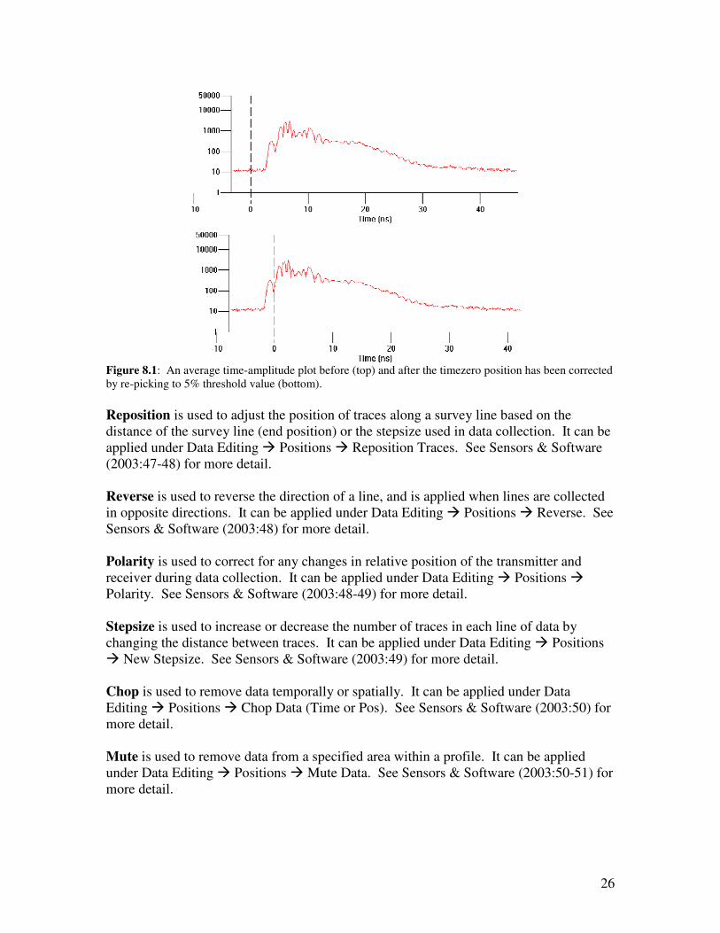
Chapter 8. Basic Data Editing Procedures Basic Data Editing in EKKO View Deluxe All of the basic data editing steps described below can be applied in EKKO View Deluxe. Data Collection Parameters can be edited under Data Editing � Header File. Parameters which can be changed include antenna separation, units, frequency, pulser voltage, and survey mode (reflection survey, CMP survey, and transillumination survey – ZOP, MOG, or VRP). See Sensors & Software (2003:44-47) for more detail. Time Window length can be changed under Data Editing � Time Window � New Time Window. See Sensors & Software (2003:52) for more detail. Points/Trace can be adjusted by selecting a different time interval (resample) or by reducing the number of points per trace (decimate). These can be applied under Data Editing � Points/Trace � Resample or Decimate. See Sensors & Software (2003:53) for more detail. Timezero can be adjusted using three methods: re-pick, datum, and edit. Offset between timezero and the first reflection should be corrected for by adjusting traces to a common timezero point that occurs at the first arrival time. Adjusting timezero is necessary for achieving correct two-way travel times and depths, and should be applied before other processing methods. See Cassidy (2009a:150-151), Conyers (2004:122), and Sensors & Software (2003:53-55) for more detail. Re-pick Timezero selects a new timezero point at the first location in the trace that exceeds a specified threshold value, or percentage of the peak amplitude. It can be applied under Data Editing � Timezero � Re-pick Timezero. Traces should be examined visually to determine a correct threshold value, which is generally 5-10%. See Sensors & Software (2003:53-54) for more detail. Datum Timezero is used to shift timezero in all traces to a horizontal datum. As in re-pick timezero, the correct timezero position is selected from the first trace based on a specified threshold value. It can be applied under Data Editing � Timezero � Datum Timezero. See Sensors & Software (2003:54-55) for more detail. Edit Timezero is used to manually calculate and input the timezero point. The timezero point is calculated by dividing the time from the beginning of the trace to timezero by the sampling interval and multiplying by 1000. It can be applied under Data Editing � Timezero � Edit. See Sensors & Software (2003:55) for more detail.

26

Figure 8.1: An average time-amplitude plot before (top) and after the timezero position has been corrected by re-picking to 5% threshold value (bottom). Reposition is used to adjust the position of traces along a survey line based on the distance of the survey line (end position) or the stepsize used in data collection. It can be applied under Data Editing � Positions � Reposition Traces. See Sensors & Software (2003:47-48) for more detail. Reverse is used to reverse the direction of a line, and is applied when lines are collected in opposite directions. It can be applied under Data Editing � Positions � Reverse. See Sensors & Software (2003:48) for more detail. Polarity is used to correct for any changes in relative position of the transmitter and receiver during data collection. It can be applied under Data Editing � Positions � Polarity. See Sensors & Software (2003:48-49) for more detail. Stepsize is used to increase or decrease the number of traces in each line of data by changing the distance between traces. It can be applied under Data Editing � Positions � New Stepsize. See Sensors & Software (2003:49) for more detail. Chop is used to remove data temporally or spatially. It can be applied under Data Editing � Positions � Chop Data (Time or Pos). See Sensors & Software (2003:50) for more detail. Mute is used to remove data from a specified area within a profile. It can be applied under Data Editing � Positions � Mute Data. See Sensors & Software (2003:50-51) for more detail.

27

Insert is used to insert blank traces where traces have been skipped, thereby keeping trace position spatially consistent. It can be applied under Data Editing � Positions � Insert Traces. See Sensors & Software (2003:51) for more detail. Delete is used to delete specific traces in a profile. It can be applied under Data Editing � Positions � Delete Traces. See Sensors & Software (2003:52) for more detail. Fill Gaps is used to interpolate traces in any gaps in the data where traces have been skipped. It can be applied under Data Editing � Positions � Fill Data Gaps. See Sensors & Software (2003:52) for more detail. Merge is used to combine two data files into a single horizontally continuous file, and is useful in reconstructing interrupted survey lines collected in two or more surveys saved as separate files. All files to be merged should have been collected using the same data collection parameters. Merge can be selected under Data Editing � File � Merge. See Sensors & Software (2003:29) for more detail. Stack is used to combine two data files into a single vertically continuous file, and is useful in comparing data lines. All files to be stacked should have been collected using the same data collection parameters. Stack can be selected under Data Editing � File � Stack. See Sensors & Software (2003:29-30) for more detail. Convert is used to convert Sensors & Software DT1 binary data files and/or ASCII header files to other formats, including SEG-Y (.SGY) and EAVESDROPPER (.EAV) for seismic processing; ASCII 1 (.AS1); ASCII 2 (.AS2) for 2D visualization and spreadsheets; and CSV (.CSV) for spreadsheets. Convert can also be used to export time or depth slices as CSV files for viewing in spreadsheet format. Convert can be selected under Data Editing � File � Convert. See Sensors & Software (2003:31-35) for more detail. Correcting for Topography and Horizontal Scaling Topographic (or static) correction is an essential component of GPR data editing, especially in cases where there is significant topographic variation. This type of editing can require the use of many programs, including EKKO View Deluxe, EKKO Mapper, and various spreadsheets and mapping programs. A number of methods of correcting for both topography and horizontal scaling are outlined below. In EKKO View Deluxe, GPS Data can be added with three methods: GPS on DVL, user GPS file, or time stamp. GPS on DVL method involves connecting a GPS unit to the GPR DVL for data acquisition, at which time GPS data is saved on the DVL as a GPS data file (.GPS) at the same time as GPR data. These files are saved in the same folder as GPR data, and can be added to individual or multiple lines of data under Data Editing � File � Add GPS Data � GPS on DVL Method. If adding multiple lines of data at once, the file names for both

28

GPS and GPR data must be the same. Note that GPS data collection parameters must be set on the DVL. See Sensors & Software (2003:38-40) for more detail. Time Stamp method records the times at which GPR and GPS data are recorded, and uses these times to correlate GPS and GPR data. This method is predominantly used when GPS is not integrated with the GPR DVL, but data is collected at the same time from another computer. GPS data must first be reformatted under Utility � GPS Tools � Reformat GPS file. The reformatted file can be added under Data Editing � File � Add GPS Data � Time Stamp Method. See Sensors & Software (2003:42-44) for more detail. User GPS File method involves manually creating a text file with a .GTP extension and adding this to individual or multiple lines of data under Data Editing � File � Add GPS Data � User GPS File Method. See Sensors & Software (2003:40-42) for more detail. GTP files (.GTP) list the GPS latitude, longitude, elevation, and trace number for each line of data, and can be created in Microsoft Windows Notepad. To save the file with a .GTP extension, save the file name in quotation marks (“gps.GTP”). Data in GTP files should be listed in the following format (excluding headings): trace / longitude (DDDMM.MM) / latitude (DDMM.MM) / elevation 1 11045.78 4327.68 1030 500 11045.79 4327.68 1024 1000 11045.80 4327.69 1010 Static Correction is used to correct for changes in topography over the survey. In some cases, applying static correction can also adjust for changes caused by difference in antenna coupling and tilt or lateral velocity variations (Goodman et al. 2006:158). In EKKO View Deluxe, topography data may be added under Data Editing � File � Add Topography using Topo File by manually creating a topo file (.TOP) with position and elevation data for each line of data (see below). Topography data may also be added under Data Editing � File � Add Topography using GPS Z, which requires adding a GPS file (see above) and specifying the GPS receiver height above the ground. In both methods, topography must be shifted under Data Editing � File � Shift Topography before effects can be visualized. See Cassidy (2009a:159-161), Conyers (2004:123), and Sensors & Software (2003:35-37) for more detail. Topo files (.TOP) list the position and elevation values, and can be created in Notepad. To save the file with a .TOP extension, save the file name in quotation marks (“elevation.top”). Position and elevation data should be listed in the following format (excluding headings): position / elevation 0 50 10 55 20 70 30 60 For instances where the exact position and location of topographic points are unknown, and/or where an extensive database of topographic points for the survey area exists, topo files can be most easily created using a series of processes in ArcGIS, by ESRI, and

29

Surfer, by Golden Software. In ArcMap, a shapefile should first be created which includes all relevant data points. This shapefile can then be imported into Surfer and converted to a grid file under Grid � Data. In the Grid Data window, the appropriate gridding method and grid line geometry can be selected, depending on the resolution required. The grid file can then be displayed as a contour map by selecting the New Contour Map option. BLN files to specify line endpoints must then be created by digitizing the line endpoints, under Select Map � Map � Digitize (note that these endpoints can be manually digitized or their precise coordinates manually entered). To create cross-sections (.DAT files), select Grid � Slice, and enter the grid file and BLN file. These .DAT files list the position along the specified line and the elevation, as required by topo files. To create a topo file from cross-sections, open the .DAT file in Microsoft Excel using space-delimited format, copy the relevant data, and paste and save in Notepad using the instructions outlined above. At this time, slices in EKKO Mapper cannot display topographic data (as per Sensors & Software 2010, personal communication). Topography-adjusted profiles can, however, be displayed in EKKO Mapper if all the processing steps used in EKKO Mapper match those used in the topography-corrected files created in EKKO View Deluxe. Sensors & Software suggests applying dewow, background subtraction (to all traces), migration, envelope (with filter width 0 ns), and SEC gain to all lines in EKKO View Deluxe. Topographic information can then be added (note that when shifting topography, the same velocity and datum must be used for all lines). This may change the points/trace value for all lines; if so, this value will need to be recalculated manually, such that all lines have the same points/trace value. Once this step has been completed, a new GFP file must be created in GFP edit using the edited data. Upon opening this GFP file in EKKO Mapper, open the data processing window and turn OFF all processes applied in EKKO View Deluxe (background subtraction, dewow, migration, envelope, and amplitude equalization gain). Rubber-Banding is used to correct the horizontal scale by stretching or squeezing the data file between manually placed fiducial markers of known spatial position. This operation is easiest to apply if fiducial marks are spaced at a constant interval (constant fid separation method), but can also be applied using an ASCII file (ASCII fid position file method) for fiducial marks spaced at varying intervals. Rubber-banding can be selected under Data Editing � File � Rubber Band. See Conyers (2004:32, 83) and Sensors & Software (2003:30-31) for more detail.

30

Basic Data Editing in GFP Edit All of the basic data editing steps described below can be applied in GFP Edit. The Orientation Tab in the Editing window gives options for changing the line type (x or y), orientation (forward or reverse), and ordering (flip x or y) of GPR data lines. See Sensors & Software (2007b:14-17, 25) for more detail. The Position Tab in the Editing window is used to move lines to a new position. This is especially useful in repositioning reversed lines, editing broken lines, and creating multiple data grids. See Sensors & Software (2007b:18, 28-32) for more detail. The Length and Step Size Tabs in the Editing window are used to alter line length by changing the step size between traces. Note that this operation does not remove data, but acts as a simple ‘rubber-banding’ operation. See Sensors & Software (2007b:19-20) for more detail. The Line Spacing Tab in the Editing window is used to define the distance between GPR data lines. See Sensors & Software (2007b:21, 26-27, 31) for more detail.

31

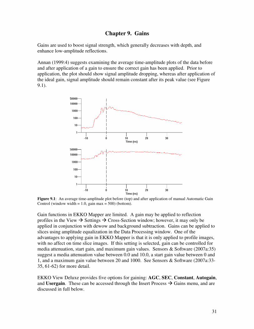
Chapter 9. Gains Gains are used to boost signal strength, which generally decreases with depth, and enhance low-amplitude reflections. Annan (1999:4) suggests examining the average time-amplitude plots of the data before and after application of a gain to ensure the correct gain has been applied. Prior to application, the plot should show signal amplitude dropping, whereas after application of the ideal gain, signal amplitude should remain constant after its peak value (see Figure 9.1).

Figure 9.1: An average time-amplitude plot before (top) and after application of manual Automatic Gain Control (window width = 1.0, gain max = 500) (bottom). Gain functions in EKKO Mapper are limited. A gain may be applied to reflection profiles in the View � Settings � Cross-Section window; however, it may only be applied in conjunction with dewow and background subtraction. Gains can be applied to slices using amplitude equalization in the Data Processing window. One of the advantages to applying gain in EKKO Mapper is that it is only applied to profile images, with no affect on time slice images. If this setting is selected, gain can be controlled for media attenuation, start gain, and maximum gain values. Sensors & Software (2007a:35) suggest a media attenuation value between 0.0 and 10.0, a start gain value between 0 and 1, and a maximum gain value between 20 and 1000. See Sensors & Software (2007a:33-35, 61-62) for more detail. EKKO View Deluxe provides five options for gaining: AGC, SEC, Constant, Autogain, and Usergain. These can be accessed through the Insert Process � Gains menu, and are discussed in full below.

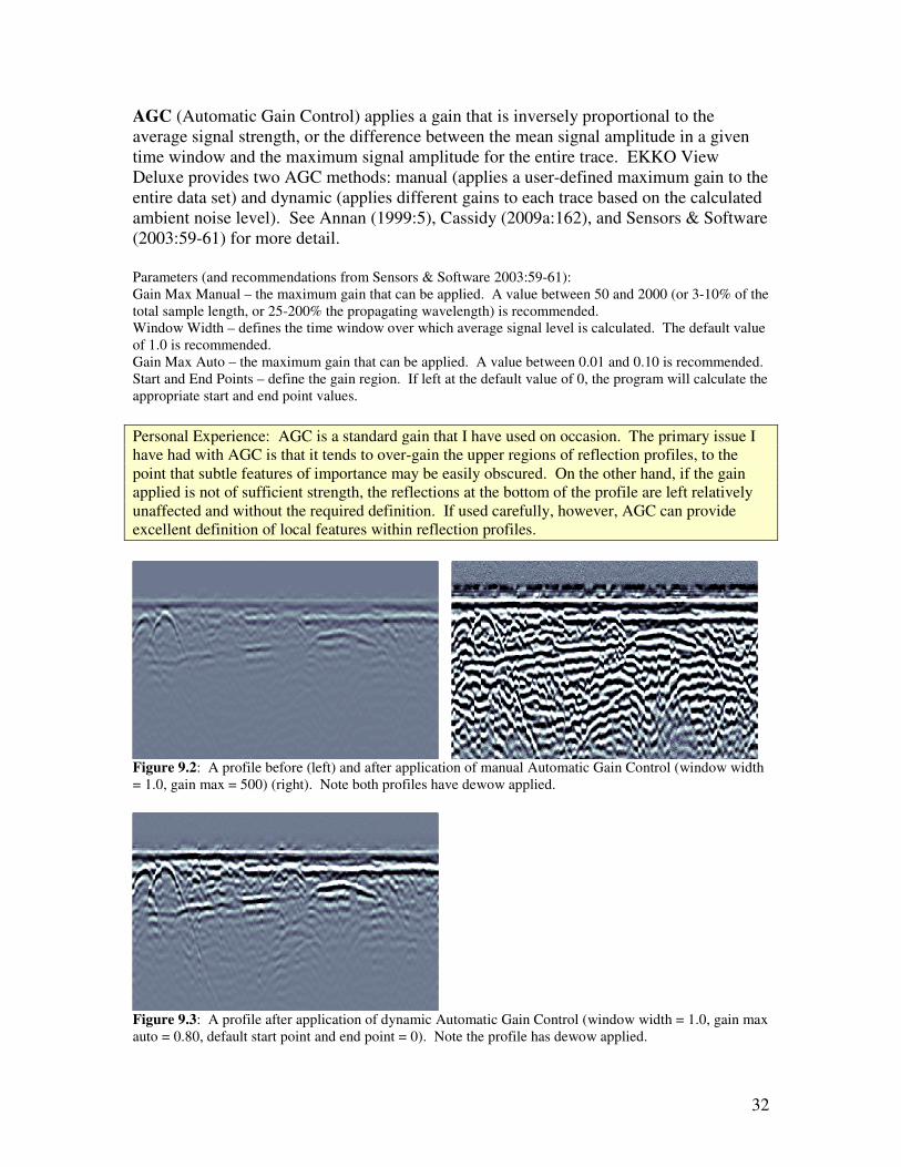
32

AGC (Automatic Gain Control) applies a gain that is inversely proportional to the average signal strength, or the difference between the mean signal amplitude in a given time window and the maximum signal amplitude for the entire trace. EKKO View Deluxe provides two AGC methods: manual (applies a user-defined maximum gain to the entire data set) and dynamic (applies different gains to each trace based on the calculated ambient noise level). See Annan (1999:5), Cassidy (2009a:162), and Sensors & Software (2003:59-61) for more detail. Parameters (and recommendations from Sensors & Software 2003:59-61): Gain Max Manual – the maximum gain that can be applied. A value between 50 and 2000 (or 3-10% of the total sample length, or 25-200% the propagating wavelength) is recommended. Window Width – defines the time window over which average signal level is calculated. The default value of 1.0 is recommended. Gain Max Auto – the maximum gain that can be applied. A value between 0.01 and 0.10 is recommended. Start and End Points – define the gain region. If left at the default value of 0, the program will calculate the appropriate start and end point values. Personal Experience: AGC is a standard gain that I have used on occasion. The primary issue I have had with AGC is that it tends to over-gain the upper regions of reflection profiles, to the point that subtle features of importance may be easily obscured. On the other hand, if the gain applied is not of sufficient strength, the reflections at the bottom of the profile are left relatively unaffected and without the required definition. If used carefully, however, AGC can provide excellent definition of local features within reflection profiles.

Figure 9.2: A profile before (left) and after application of manual Automatic Gain Control (window width = 1.0, gain max = 500) (right). Note both profiles have dewow applied.

Figure 9.3: A profile after application of dynamic Automatic Gain Control (window width = 1.0, gain max auto = 0.80, default start point and end point = 0). Note the profile has dewow applied.

33

SEC (Spreading & Exponential Compensation or energy decay) gain applies an exponential gain (approximately 1/r2) that compensates for the spreading and attenuation of the propagating wavefront. EKKO View Deluxe provides two SEC gain methods: manual and auto. See Cassidy (2009a:162), Leckebusch (2003:217), and Sensors & Software (2003:62-64) for more detail. Leckebusch (2003:217) recommends use of SEC over AGC, as the latter distorts relative amplitudes. Parameters (and recommendations from Sensors & Software 2003:62-64): Gain Max Manual – the maximum gain that can be applied. A value between 50 and 2000 is recommended. Start Value – a constant added to the exponential gain function. A value between 0 and 10 is recommended. Attenuation – the attenuation value (in dB/m) of the substrate. A value between 0.5 and 5 is typical. Gain Max Auto – the maximum gain that can be applied. A value between 0.01 and 0.10 is recommended. Start and End Points – define the gain region. If left at the default value of 0, the program will calculate the appropriate start and end point values. Personal Experience: SEC is by far my preferred gaining method. It is far easier to control than AFC as far as over-gaining is concerned, and tends to produce a more balanced reflection profile. The definition of more subtle features can be compromised, but there are other methods available to bring these features to the forefront.

Figure 9.4: A profile before (left) and after application of manual SEC gain (attenuation = 1.5, start value = 1.0, gain max = 500) (right). Note both profiles have dewow applied.

Figure 9.5: A profile after application of manual SEC gain (attenuation = 5.0, start value = 1.0, gain max = 500) (left) and after application of auto SEC gain (attenuation = 5.0, start value = 1.0, gain max auto = 0.80, default start point and end point = 0). Note both profiles have dewow applied.

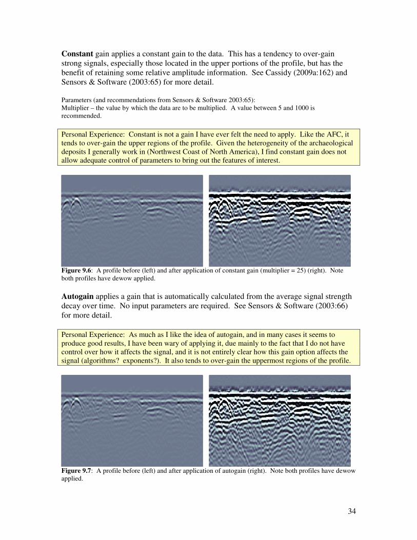
34

Constant gain applies a constant gain to the data. This has a tendency to over-gain strong signals, especially those located in the upper portions of the profile, but has the benefit of retaining some relative amplitude information. See Cassidy (2009a:162) and Sensors & Software (2003:65) for more detail. Parameters (and recommendations from Sensors & Software 2003:65): Multiplier – the value by which the data are to be multiplied. A value between 5 and 1000 is recommended. Personal Experience: Constant is not a gain I have ever felt the need to apply. Like the AFC, it tends to over-gain the upper regions of the profile. Given the heterogeneity of the archaeological deposits I generally work in (Northwest Coast of North America), I find constant gain does not allow adequate control of parameters to bring out the features of interest.

Figure 9.6: A profile before (left) and after application of constant gain (multiplier = 25) (right). Note both profiles have dewow applied. Autogain applies a gain that is automatically calculated from the average signal strength decay over time. No input parameters are required. See Sensors & Software (2003:66) for more detail. Personal Experience: As much as I like the idea of autogain, and in many cases it seems to produce good results, I have been wary of applying it, due mainly to the fact that I do not have control over how it affects the signal, and it is not entirely clear how this gain option affects the signal (algorithms? exponents?). It also tends to over-gain the uppermost regions of the profile.

Figure 9.7: A profile before (left) and after application of autogain (right). Note both profiles have dewow applied.

35

Usergain applies a custom user-defined gain from a tabulated gain function file (ASCII format with extension .GAN). The file must contain time and gain data, which are then imported and linearly interpolated to apply a gain to the entire data set. This option allows different gain values to be applied to different specified time windows across the data set. See Cassidy (2009a:162) and Sensors & Software (2003:67) for more detail. Gain files (.GAN) list the time and gain values, and can be created in Notepad. To save the file with a .GAN extension, save the file name in quotation marks (“usergain.gan”). Time and gain data should be listed in the following format (excluding headings): time / gain 10 10 20 20 30 5 Personal Experience: I have never used usergain, mainly due to the increased time and efforts needed to create and apply gain files. For the purposes of my work, and the overall heterogeneity of the research contexts, multiple gain files would be required to produce adequate results. Usergain is thus an inefficient processing method in my own research contexts.

Figure 9.8: A profile before (left) and after application of usergain (time and gain values listed in sample .GAN file above) (right). Note both profiles have dewow applied.

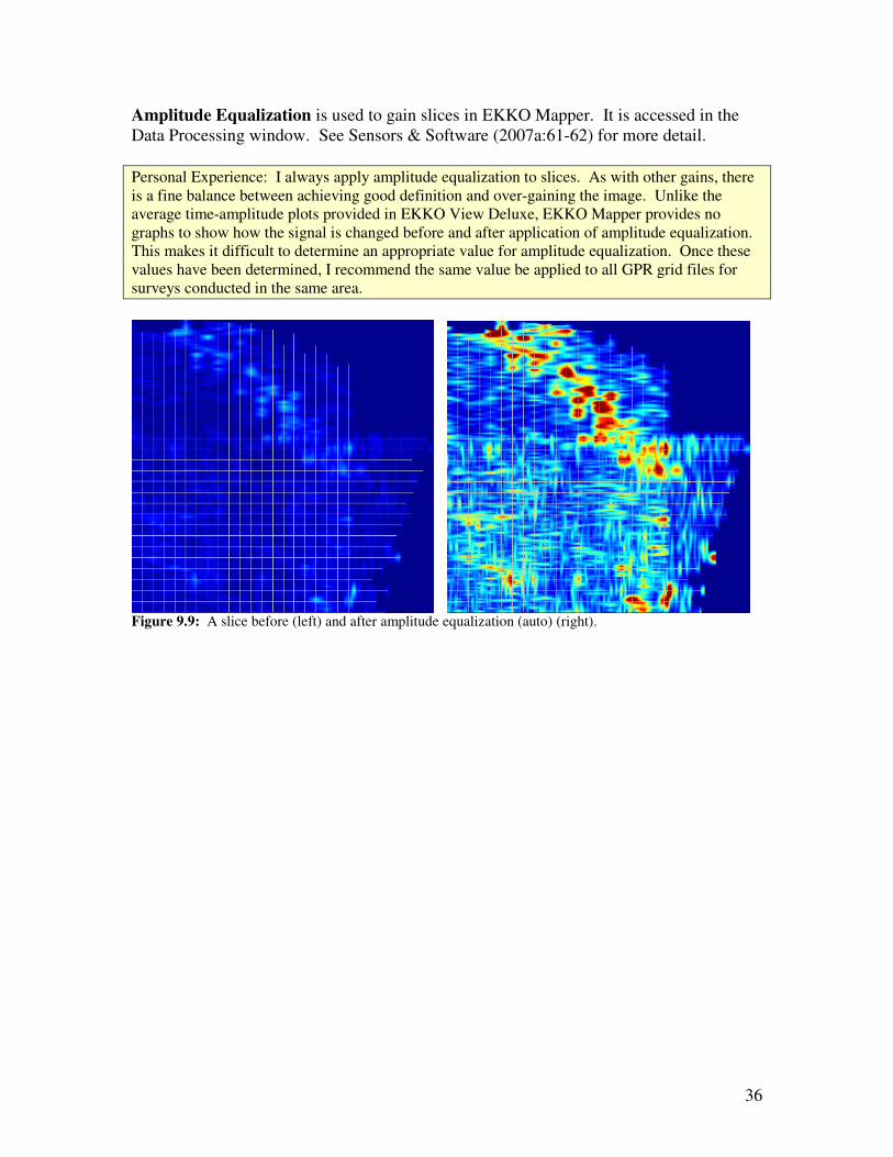
36

Amplitude Equalization is used to gain slices in EKKO Mapper. It is accessed in the Data Processing window. See Sensors & Software (2007a:61-62) for more detail. Personal Experience: I always apply amplitude equalization to slices. As with other gains, there is a fine balance between achieving good definition and over-gaining the image. Unlike the average time-amplitude plots provided in EKKO View Deluxe, EKKO Mapper provides no graphs to show how the signal is changed before and after application of amplitude equalization. This makes it difficult to determine an appropriate value for amplitude equalization. Once these values have been determined, I recommend the same value be applied to all GPR grid files for surveys conducted in the same area.

Figure 9.9: A slice before (left) and after amplitude equalization (auto) (right).

37

Chapter 10. Time Filters Time filters alter the shape of single traces in the vertical (temporal) direction to enhance or eliminate certain frequencies and features. Annan (1999:5) suggests examining an average amplitude spectrum plot before and after applying a filter to aid in determining filter parameters. Prior to application, the plot should show an irregular curve representing the frequencies present in the signal. Examining the plot again after application of a filter will show which frequencies have been removed from the spectrum (see Figure 10.1).

Figure 10.1: An average amplitude spectrum plot before (top) and after application of a lowpass filter (cutoff percent = 20%) (bottom). Only dewow is available in EKKO Mapper, and may be applied in the Tool � Data Processing window, under the subheading DME Processing. EKKO View Deluxe provides eight options for temporal filtering: Dewow, DC Shift, Bandpass, Lowpass, Highpass, Vertical, Median, and Deconvolution. These can be accessed through the Insert Process � Time Filters menu, and are discussed in full below.

38

Dewow (or signal saturation correction) applies a running average filter to each trace to remove the initial DC signal component and low-frequency “wow,” which is caused by signal saturation due to early wave arrivals, inductive coupling effects, and/or instrumentation dynamic range limitations. It is highly recommended dewow be applied to all data sets before other processing steps are undertaken. No input parameters are required. See Annan (1999:4), Cassidy (2009a:150), and Sensors & Software (2003:68-69; 2007a:55) for more detail. Personal Experience: I always use dewow, and strongly recommend it be applied to all data sets.

Figure 10.2: A profile before (left) and after application of dewow (right) in EKKO View Deluxe. Note both profiles have gain applied. DC Shift removes a constant DC level from each trace. It may be used in addition to or as a substitution for dewow. EKKO View Deluxe provides two DC Shift methods: manual and program calculated. Manual DC Shift removes the same DC level from every trace, whereas program calculated DC Shift removes a program calculated DC level unique to each trace. See Sensors & Software (2003:70-71) for more detail. Parameters (and recommendations from Sensors & Software 2003:70-71): DC Level – constant to be subtracted from the data. Start and End Points – define the window from which the DC level to be subtracted is calculated. If left at the default value of 0, the program will calculate the DC level from all points in each trace. Personal Experience: I have never felt the need to use DC Shift.

Figure 10.3: A profile after application of a manual DC Shift (DC level = 500) (left) and after application of program calculated DC Shift (start point = end point = 0) (right). Note both profiles have gain applied.

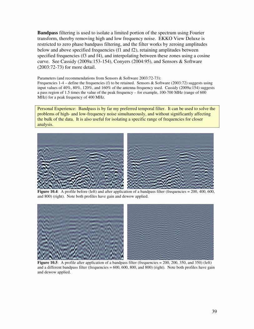
39

Bandpass filtering is used to isolate a limited portion of the spectrum using Fourier transform, thereby removing high and low frequency noise. EKKO View Deluxe is restricted to zero phase bandpass filtering, and the filter works by zeroing amplitudes below and above specified frequencies (f1 and f2), retaining amplitudes between specified frequencies (f3 and f4), and interpolating between these zones using a cosine curve. See Cassidy (2009a:153-154), Conyers (2004:95), and Sensors & Software (2003:72-73) for more detail. Parameters (and recommendations from Sensors & Software 2003:72-73): Frequencies 1-4 – define the frequencies (f) to be retained. Sensors & Software (2003:72) suggests using input values of 40%, 80%, 120%, and 160% of the antenna frequency used. Cassidy (2009a:154) suggests a pass region of 1.5 times the value of the peak frequency – for example, 100-700 MHz (range of 600 MHz) for a peak frequency of 400 MHz. Personal Experience: Bandpass is by far my preferred temporal filter. It can be used to solve the problems of high- and low-frequency noise simultaneously, and without significantly affecting the bulk of the data. It is also useful for isolating a specific range of frequencies for closer analysis.

Figure 10.4: A profile before (left) and after application of a bandpass filter (frequencies = 200, 400, 600, and 800) (right). Note both profiles have gain and dewow applied.

Figure 10.5: A profile after application of a bandpass filter (frequencies = 200, 200, 350, and 350) (left) and a different bandpass filter (frequencies = 600, 600, 800, and 800) (right). Note both profiles have gain and dewow applied.

40

Lowpass filtering removes the high frequency signal content in the temporal dimension. It is used to remove high-frequency noise or “snow.” See Cassidy (2009a:153), Conyers (2004:96, 120), and Sensors & Software (2003:74) for more detail. Parameters (and recommendations from Sensors & Software 2003:74): Cutoff Percent –the frequency above which data are removed (must be between 10% and 90%). Personal Experience: I rarely use lowpass, as the desired effects (generally removing high-frequency noise or isolating low-frequency signals) can be achieved in bandpass instead.

Figure 10.6: A profile before (left) and after application of a lowpass filter (cutoff percent = 10%) (right). Note both profiles have gain and dewow applied. Highpass filtering removes the low frequency signal content in the temporal dimension. It is used to remove low frequency data and horizontal banding due to system noise. See Cassidy (2009a:153), Conyers (2004:96, 120), and Sensors & Software (2003:75) for more detail. Parameters (and recommendations from Sensors & Software 2003:75): Cutoff Percent –the frequency above which data are preserved (must be between 10% and 90%). Personal Experience: I rarely use highpass, as the desired effects (generally removing low-frequency noise or isolating high-frequency signals) can be achieved in bandpass instead.

Figure 10.7: A profile before (left) and after application of a highpass filter (cutoff percent = 20%) (right). Note both profiles have gain and dewow applied.

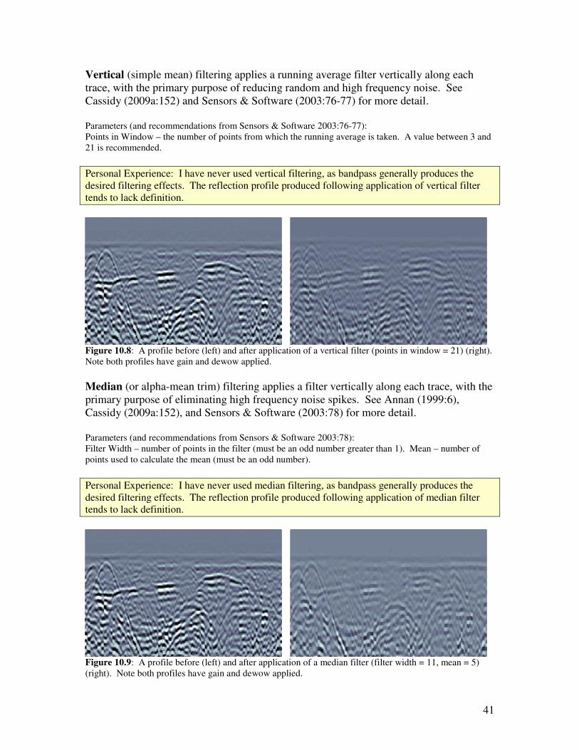
41

Vertical (simple mean) filtering applies a running average filter vertically along each trace, with the primary purpose of reducing random and high frequency noise. See Cassidy (2009a:152) and Sensors & Software (2003:76-77) for more detail. Parameters (and recommendations from Sensors & Software 2003:76-77): Points in Window – the number of points from which the running average is taken. A value between 3 and 21 is recommended. Personal Experience: I have never used vertical filtering, as bandpass generally produces the desired filtering effects. The reflection profile produced following application of vertical filter tends to lack definition.

Figure 10.8: A profile before (left) and after application of a vertical filter (points in window = 21) (right). Note both profiles have gain and dewow applied. Median (or alpha-mean trim) filtering applies a filter vertically along each trace, with the primary purpose of eliminating high frequency noise spikes. See Annan (1999:6), Cassidy (2009a:152), and Sensors & Software (2003:78) for more detail. Parameters (and recommendations from Sensors & Software 2003:78): Filter Width – number of points in the filter (must be an odd number greater than 1). Mean – number of points used to calculate the mean (must be an odd number). Personal Experience: I have never used median filtering, as bandpass generally produces the desired filtering effects. The reflection profile produced following application of median filter tends to lack definition.

Figure 10.9: A profile before (left) and after application of a median filter (filter width = 11, mean = 5) (right). Note both profiles have gain and dewow applied.

42

Deconvolution is an inverse temporal filter that compresses the recorded wavelets, thereby improving data resolution. It can be used to remove multiples (repetitive horizontal reflections spaced at equal intervals) formed by multiple reflections between the surface and subsurface objects or layers, and convert radar wavelets to spikes. The deconvolution algorithm relies on the assumptions that subsurface layering is horizontal with uniform intra-layer velocities, and that reflected waveforms have regular signals that do not scatter energy. See Annan (1999:8-9), Cassidy (2009a:158), Conyers (2004:120, 126-128), and Sensors & Software (2003:79) for more detail. Annan (1999:8-9) notes that deconvolution is “not straight forward and has seldom yielded a great deal of benefit”; and that it “can be both difficult to apply systematically and exhibit little enhancement in resolution.” Likewise, Conyers (2004:128) notes that “much about this processing technique still remains obscure” and recent examples of its use have been “unsatisfactory.” Orlando (2007:214) indicates that deconvolution “gives very poor results.” It is suggested that deconvolution is most beneficial when extraneous and system reverberations are present (Annan 1999:9). Parameters (and recommendations from Sensors & Software 2003:79): Frequency – GPR centre frequency. Filter Width – width of the filter. Delay – time lag between the input signal and output spike (0.5 times the filter width). Spike Width – width of the output spike. Whiten – factor to stabilize the filter (must be between 0 and 1). Personal Experience: As with Annan, Conyers, and Orlando (above), I have had less than satisfactory results with deconvolution. I would recommend against its use.

Figure 10.10: A profile before (left) and deconvolution (default values: frequency = filter width = delay = spike width = whitening = 0) (right). Note both profiles have gain and dewow applied.

43

Chapter 11. Spatial Filters Spatial filters alter the shape of adjacent traces in the horizontal (spatial) direction to enhance or eliminate certain frequencies and features. Annan (1999:6) suggests examining an average amplitude spectrum plot before and after applying a filter to aid in determining filter parameters. Prior to application, the plot should show an irregular curve representing the frequencies present in the signal; examining the plot again after application of a filter will show which frequencies have been removed from the spectrum (see Figure 11.1).

Figure 11.1: An average amplitude spectrum plot before (top) and after application of a lowpass filter (cutoff percent = 20%) (bottom). Only background subtraction is available in EKKO Mapper. It may be applied in the Tool � Data Processing window, under the subheading Background Subtraction; note however that it must be used in conjunction with dewow. EKKO View Deluxe provides seven options for spatial filtering: Background Subtraction, Horizontal, Binomial, Lowpass, Highpass, Median, and Trace Difference. These can be accessed through the Insert Process � Spatial Filters menu, and are discussed in full below.

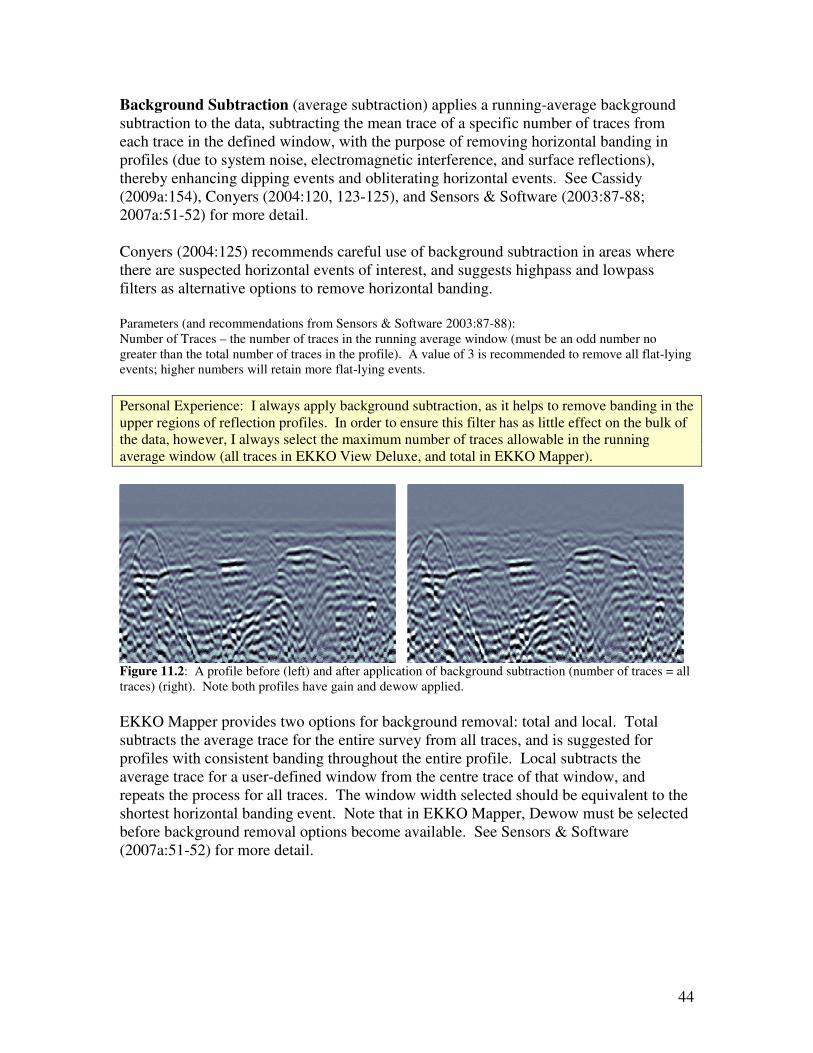
44

Background Subtraction (average subtraction) applies a running-average background subtraction to the data, subtracting the mean trace of a specific number of traces from each trace in the defined window, with the purpose of removing horizontal banding in profiles (due to system noise, electromagnetic interference, and surface reflections), thereby enhancing dipping events and obliterating horizontal events. See Cassidy (2009a:154), Conyers (2004:120, 123-125), and Sensors & Software (2003:87-88; 2007a:51-52) for more detail. Conyers (2004:125) recommends careful use of background subtraction in areas where there are suspected horizontal events of interest, and suggests highpass and lowpass filters as alternative options to remove horizontal banding. Parameters (and recommendations from Sensors & Software 2003:87-88): Number of Traces – the number of traces in the running average window (must be an odd number no greater than the total number of traces in the profile). A value of 3 is recommended to remove all flat-lying events; higher numbers will retain more flat-lying events. Personal Experience: I always apply background subtraction, as it helps to remove banding in the upper regions of reflection profiles. In order to ensure this filter has as little effect on the bulk of the data, however, I always select the maximum number of traces allowable in the running average window (all traces in EKKO View Deluxe, and total in EKKO Mapper).

Figure 11.2: A profile before (left) and after application of background subtraction (number of traces = all traces) (right). Note both profiles have gain and dewow applied. EKKO Mapper provides two options for background removal: total and local. Total subtracts the average trace for the entire survey from all traces, and is suggested for profiles with consistent banding throughout the entire profile. Local subtracts the average trace for a user-defined window from the centre trace of that window, and repeats the process for all traces. The window width selected should be equivalent to the shortest horizontal banding event. Note that in EKKO Mapper, Dewow must be selected before background removal options become available. See Sensors & Software (2007a:51-52) for more detail.

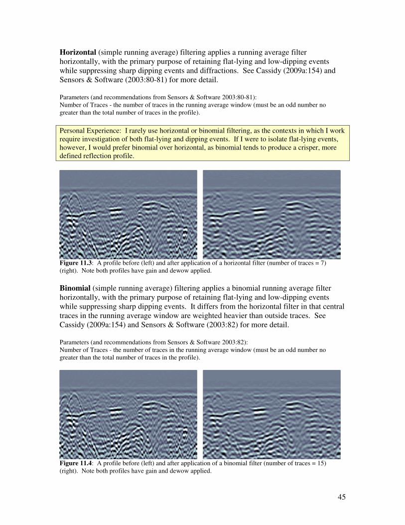
45

Horizontal (simple running average) filtering applies a running average filter horizontally, with the primary purpose of retaining flat-lying and low-dipping events while suppressing sharp dipping events and diffractions. See Cassidy (2009a:154) and Sensors & Software (2003:80-81) for more detail. Parameters (and recommendations from Sensors & Software 2003:80-81): Number of Traces - the number of traces in the running average window (must be an odd number no greater than the total number of traces in the profile). Personal Experience: I rarely use horizontal or binomial filtering, as the contexts in which I work require investigation of both flat-lying and dipping events. If I were to isolate flat-lying events, however, I would prefer binomial over horizontal, as binomial tends to produce a crisper, more defined reflection profile.

Figure 11.3: A profile before (left) and after application of a horizontal filter (number of traces = 7) (right). Note both profiles have gain and dewow applied. Binomial (simple running average) filtering applies a binomial running average filter horizontally, with the primary purpose of retaining flat-lying and low-dipping events while suppressing sharp dipping events. It differs from the horizontal filter in that central traces in the running average window are weighted heavier than outside traces. See Cassidy (2009a:154) and Sensors & Software (2003:82) for more detail. Parameters (and recommendations from Sensors & Software 2003:82): Number of Traces - the number of traces in the running average window (must be an odd number no greater than the total number of traces in the profile).

Figure 11.4: A profile before (left) and after application of a binomial filter (number of traces = 15) (right). Note both profiles have gain and dewow applied.

46

Lowpass filtering removes the high frequency signal content in the temporal dimension. It is used to enhance flat-lying events and slowly-changing features, and suppress dipping events. It may also aid in removing horizontal banding due to low-frequency interference. See Annan (1999:6), Cassidy (2009a:154), Conyers (2004:125), and Sensors & Software (2003:83) for more detail. Parameters (and recommendations from Sensors & Software 2003:83): Cutoff Percent –the frequency above which data are removed (must be between 10% and 90%). Personal Experience: I rarely use lowpass or highpass spatial filtering, as the contexts in which I work require investigation of both flat-lying and dipping events, and both constant and rapidly changing events. The lowpass and highpass spatial filters tend to produce the same results as the lowpass and highpass temporal filters respectively.

Figure 11.5: A profile before (left) and after application of a lowpass filter (cutoff percent = 10%) (right). Note both profiles have gain and dewow applied. Highpass filtering removes the low frequency signal content in the temporal dimension. It is used to enhance localized features and suppress flat-lying and constant events. See Annan (1999:6), Cassidy (2009a:154), and Sensors & Software (2003:84) for more detail. Parameters (and recommendations from Sensors & Software 2003:84): Cutoff Percent –the frequency above which data are preserved (must be between 10% and 90%).

Figure 11.6: A profile before (left) and after application of a highpass filter (cutoff percent = 20%) (right). Note both profiles have gain and dewow applied.

47

Median (or alpha-mean trim) filtering applies a filter vertically along each trace, with the primary purpose of eliminating high frequency noise spikes and isolated faulty traces. See Annan (1999:6) and Sensors & Software (2003:85) for more detail. Parameters (and recommendations from Sensors & Software 2003:85): Filter Width – the number of traces in the filter (must be an odd number greater than 1). Mean – the number of traces used to calculate the mean (must be an odd number). Personal Experience: I have never used median filtering, as bandpass generally produces the desired filtering effect (removing high-frequency noise). The reflection profile produced following application of median filter tends to lack definition.

Figure 11.7: A profile before (left) and after application of a median filter (filter width = 9, mean = 3) (right). Note both profiles have gain and dewow applied. Trace Difference filtering replaces each trace with the difference between itself and the previous trace, with the primary purpose of enhancing dipping (or rapidly changing) events and suppressing flat-lying (or relatively constant) events. It acts as a simplified highpass filter. No input parameters are required. See Sensors & Software (2003:86) for more detail. Personal Experience: I rarely use trace difference, as the contexts in which I work require investigation of both flat-lying and dipping events. Trace difference is roughly analogous to background subtraction with an extremely narrow running average window (one trace). The reflection profile produced following application of trace difference tends to lack definition.

Figure 11.8: A profile before (left) and after application of trace difference (right). Note both profiles have gain and dewow applied.

48

Chapter 12. 2D Filters Two-Dimensional filters (e.g., t-x average or t-x median filters) operate in both the temporal and spatial directions, usually with results similar to their one-dimensional temporal or spatial counterparts. They are most often used to remove noise and spikes. See Cassidy (2009a:157) for more detail. Only migration is available in EKKO Mapper, and may be applied in the Tool � Data Processing window, under the subheading DME Processing. EKKO View Deluxe provides two options for 2D filtering: Migration and Dip. These can be accessed through the Insert Process � 2D Filters menu, and are discussed in full below. Dip filtering is used to enhance dipping events at a specified dip angle. See Sensors & Software (2003:90) for more detail. Parameters (and recommendations from Sensors & Software 2003:90): Dip Slope – the slope angle to be enhanced (must be between -30 and +30). Filter Width – the filter width in number of traces. Scale – a constant multiplier to reduce gaining effects caused by the dip filter process (must be between 0.01 and 1.0). Personal Experience: I rarely use dip, as the contexts in which I work require investigation of both flat-lying and dipping events. For most heterogeneous archaeological contexts, this filter option seems irrelevant; it is likely more applicable to geological research on dipping strata.

Figure 12.1: A profile before (left) and after application of a dip filter (dip slope = 25 and -25, filter width = 5, scale = 1) (right). Note both profiles have gain and dewow applied.

49

Migration applies a synthetic aperture image reconstruction process to focus scattered signals, collapse hyperbolas to their apices, and reposition dipping reflections. Migration requires an accurate radar velocity and knowledge of the origin of the distorted reflections and wave travel paths before it can be applied to the data. It operates on a number of assumptions, including constant laterally invariant velocity layers; spatially uniform and spherically propagating source; no antenna separation; and no dispersion or attenuation. See Annan (1999:11), Cassidy (2009a:164-166), Conyers (2004:120, 128-129), Leckebusch (2003:218), Orlando (2007:219), and Sensors & Software (2003:89; 2007a:56) for more detail. Leckebusch (2003:218) notes no difference between Kirchhoff, Stolt (F-K), phase-shift, and finite-difference migration (wave equation) methods. Annan (1999:11) warns that migration may introduce false reflectors, and Conyers (2004:129) warns it may distort reflections incorrectly. One benefit to migration is increased image resolution (Orlando 2007:219), and Leckebusch (2003:218) suggests that it is only when migration is applied that exact structural dimensions can be determined. Conyers (2004:129) recommends analysing data prior to migration, as the presence of hyperbolas may aid in detecting important subsurface features. Leckebusch (2003:218) notes the correct velocity can be determined with the help of migration, as it is only at the correct velocity when ‘smileys’ appear (smileys being the inverse of the hyperbola). Parameters (and recommendations from Sensors & Software 2003:89): Velocity – the velocity of the wave through the ground. Spatial Offset – the window width for the synthetic aperture process. If left at the default value of 0, the program will calculate the appropriate spatial offset. Scale – a constant multiplier to reduce gaining effects caused by the synthetic aperture process (must be between 0.01 and 1.0). Personal Experience: I rarely use migration in EKKO View Deluxe, as the contexts in which I work require investigation of both flat-lying and dipping events. In addition, problems can arise in contexts where the deposits are heterogeneous and the velocity of the signal changes significantly over the profile, as this process assumes a constant velocity. If these changes cannot be accounted for, migration can produce distracting processing artefacts that can be mistaken for true reflections.

Figure 12.2: A profile before (left) and after migration (velocity = 0.07, spatial offset = 0, scale = 0.2) (right). Note both profiles have gain and dewow applied.

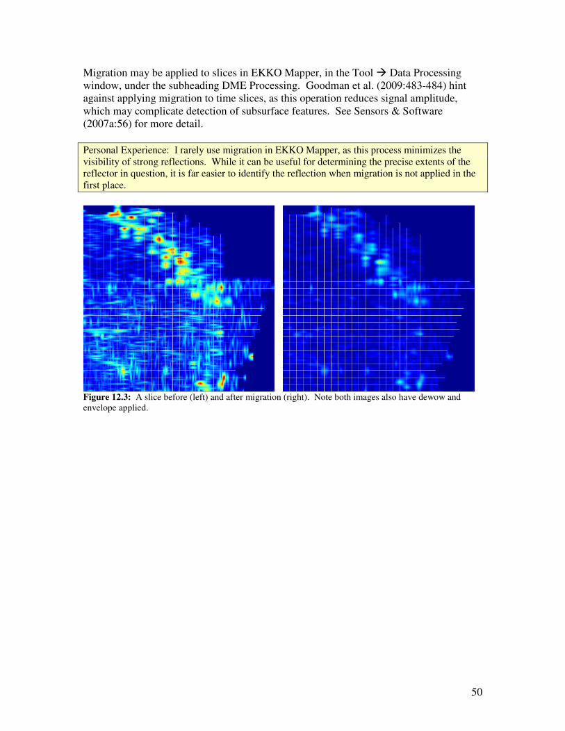
50

Migration may be applied to slices in EKKO Mapper, in the Tool � Data Processing window, under the subheading DME Processing. Goodman et al. (2009:483-484) hint against applying migration to time slices, as this operation reduces signal amplitude, which may complicate detection of subsurface features. See Sensors & Software (2007a:56) for more detail. Personal Experience: I rarely use migration in EKKO Mapper, as this process minimizes the visibility of strong reflections. While it can be useful for determining the precise extents of the reflector in question, it is far easier to identify the reflection when migration is not applied in the first place.

Figure 12.3: A slice before (left) and after migration (right). Note both images also have dewow and envelope applied.

51

Chapter 13. Attributes Attribute analysis uses imaginary components of the data (calculated using Hilbert transform) to inform on relative or instantaneous reflectivity, amplitude, frequency, and phase relationships expressed in the data. These attributes are applied to the data in a moving time-space (t-x) window to generate an attribute-based GPR section with true spatial distribution. See Annan (1999:8), Cassidy (2009a:167-168), and Sensors & Software (2003:91-94; 2007a:57-58) for more detail. Cassidy (2009a:168) warns against the use of attribute analysis in heterogeneous environments, as it can produce erroneous and inconclusive results. Only envelope is available in EKKO Mapper. It may be applied in the Tool � Data Processing window, under the subheading DME Processing. EKKO View Deluxe provides three options for attribute analysis: Envelope, Instantaneous Phase, and Instantaneous Frequency. These can be accessed through the Insert Process � Attributes menu, and are discussed in full below.

52

Envelope (instantaneous amplitude) calculates the absolute value of each wavelet by converting negative wavelets to positive wavelets, resulting in a positive monopulse wavelet. This process is used to emphasize the true resolution of the data, and can be used to simplify data and evaluate the signal strength and reflectivity. See Annan (1999:8), Cassidy (2009a:168), and Sensors & Software (2003:92-93; 2007a:57-58) for more detail. Parameters (and recommendations from Sensors & Software 2003:92-93): Filter Width – the width of the filter in nanoseconds. Personal Experience: I always apply envelope in EKKO Mapper, as it seems to amplify the results and produce more crisp slices. In EKKO View Deluxe, I prefer rectify over envelope, as it appears to retain greater horizontal continuity than envelope while producing similar results.

Figure 13.1: A profile before (left) and after application of envelope (filter width = 0.5) (right). Note both profiles have gain and dewow applied. Only envelope is available in EKKO Mapper. It may be applied in the Tool � Data Processing window, under the subheading DME Processing. It is highly recommended for slice display, as positive and negative amplitudes will readily cancel one another out. See Sensors & Software (2007a:57-58) for more detail.

Figure 13.2: A slice before (left) and after envelope (right).

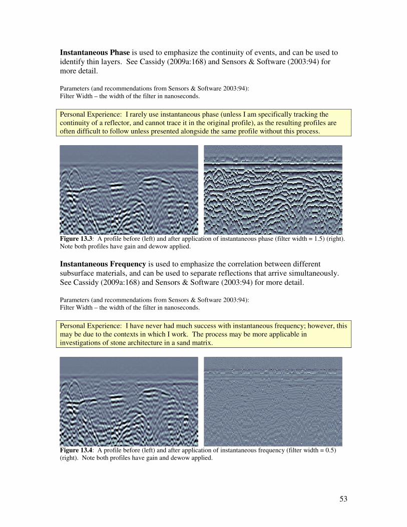
53

Instantaneous Phase is used to emphasize the continuity of events, and can be used to identify thin layers. See Cassidy (2009a:168) and Sensors & Software (2003:94) for more detail. Parameters (and recommendations from Sensors & Software 2003:94): Filter Width – the width of the filter in nanoseconds. Personal Experience: I rarely use instantaneous phase (unless I am specifically tracking the continuity of a reflector, and cannot trace it in the original profile), as the resulting profiles are often difficult to follow unless presented alongside the same profile without this process.

Figure 13.3: A profile before (left) and after application of instantaneous phase (filter width = 1.5) (right). Note both profiles have gain and dewow applied. Instantaneous Frequency is used to emphasize the correlation between different subsurface materials, and can be used to separate reflections that arrive simultaneously. See Cassidy (2009a:168) and Sensors & Software (2003:94) for more detail. Parameters (and recommendations from Sensors & Software 2003:94): Filter Width – the width of the filter in nanoseconds. Personal Experience: I have never had much success with instantaneous frequency; however, this may be due to the contexts in which I work. The process may be more applicable in investigations of stone architecture in a sand matrix.

Figure 13.4: A profile before (left) and after application of instantaneous frequency (filter width = 0.5) (right). Note both profiles have gain and dewow applied.

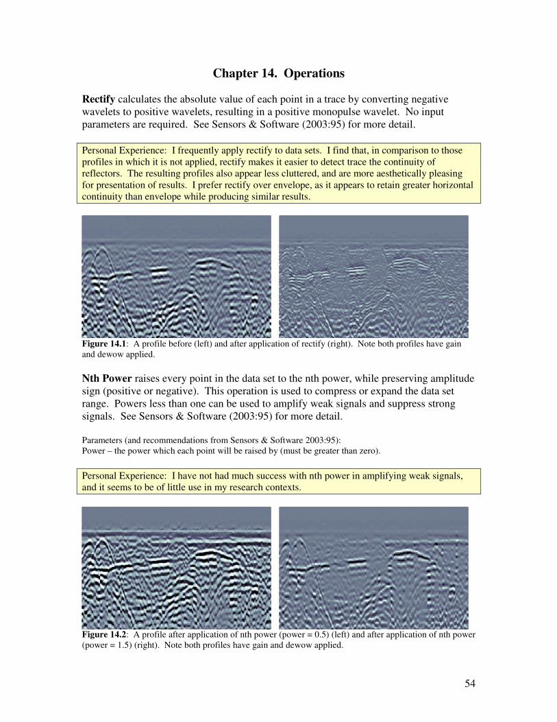
54

Chapter 14. Operations Rectify calculates the absolute value of each point in a trace by converting negative wavelets to positive wavelets, resulting in a positive monopulse wavelet. No input parameters are required. See Sensors & Software (2003:95) for more detail. Personal Experience: I frequently apply rectify to data sets. I find that, in comparison to those profiles in which it is not applied, rectify makes it easier to detect trace the continuity of reflectors. The resulting profiles also appear less cluttered, and are more aesthetically pleasing for presentation of results. I prefer rectify over envelope, as it appears to retain greater horizontal continuity than envelope while producing similar results.

Figure 14.1: A profile before (left) and after application of rectify (right). Note both profiles have gain and dewow applied. Nth Power raises every point in the data set to the nth power, while preserving amplitude sign (positive or negative). This operation is used to compress or expand the data set range. Powers less than one can be used to amplify weak signals and suppress strong signals. See Sensors & Software (2003:95) for more detail. Parameters (and recommendations from Sensors & Software 2003:95): Power – the power which each point will be raised by (must be greater than zero). Personal Experience: I have not had much success with nth power in amplifying weak signals, and it seems to be of little use in my research contexts.

Figure 14.2: A profile after application of nth power (power = 0.5) (left) and after application of nth power (power = 1.5) (right). Note both profiles have gain and dewow applied.

55

Threshold is used to zero all amplitude points below a specified input threshold, and is commonly used to emphasise high amplitude signals. See Sensors & Software (2003:96) for more detail. Parameters (and recommendations from Sensors & Software 2003:96): Cutoff Percent – the percent of the maximum threshold below which amplitudes are zeroed. Personal Experience: I have found no reason to use threshold in my research to amplify high amplitude signals.

Figure 14.3: A profile before (left) and after application of threshold (cutoff percent = 5%) (right). Note both profiles have gain and dewow applied. Amplitude Spectra is used to reveal the frequency composition of a trace by plotting amplitude versus frequency. It is commonly used to determine which filter or processing technique should be applied to the data. When displayed as a profile, the amplitude spectra shows variations in frequency over the survey line. See Sensors & Software (2003:96) for more detail. Parameters (and recommendations from Sensors & Software 2003:96): Factor – a constant multiplier. A value of 1 is recommended. Personal Experience: I’ve never found much use for amplitude spectra. If it plotted amplitude versus frequency in a different way, with labelled and numbered axes (similar to the available average time-amplitude plots), I could see it being helpful in determining processing streams.

Figure 14.4: A profile before (left) and after application of amplitude spectra (factor = 1) (right). Note both profiles have gain and dewow applied.

56

Subtract Section is used to subtract the trace of one file from the trace of the input file. It is most commonly used for subtracting processed data files from the original data files. See Sensors & Software (2003:97) for more detail. Add Section is used to add the traces of two files together. It is most commonly used (alongside Chop and Stack) to merge data files with different data collection parameters, thereby allowing display of optimal resolution versus depth. See Sensors & Software (2003:98) for more detail. Average Trace is used to calculate the average trace in a profile. This average trace may then be subtracted from a given file using the subtract section operation. See Sensors & Software (2003:98) for more detail.

57

Chapter 15. Data Processing Steps and Recommendations Cassidy (2009a:145-146) suggests four guidelines to keep in mind when processing data: (1) keep it simple; (2) keep it real; (3) understand what you are doing; and (4) be systematic and consistent. The general views expressed by Annan (1999) and Conyers (2004:131) are similar: with regards to data processing, simpler is often better, and anything more should be used with caution. Cassidy (2009a:145) adds: “ninety percent of all data collected needs only basic processing.” Annan (1999:9-12) and Cassidy (2009a:145, 158) in particular warn against use of advanced processing and visual/interpretation processing steps: while these may enhance weak signals and specific data components, they may also oversimplify reality and produce artefacts where no responses actually exist. Certain data processing steps (including dewow, migration, background removal, gain, and envelope) may affect the original signal amplitude and/or relative signal amplitudes, creating pseudo-anomalies or obscuring actual anomalies. As time slices map signal amplitude in the horizontal plane, such steps will distort amplitude values (and thus time slice images) in this plane (Annan 1999:5; Cassidy 2009a:161; Leckebusch 2003:217; Sensors & Software 2007a:49). Annan’s Recommendations Annan (1999) suggests data processing be conducted in four consecutive phases: (1) data editing; (2) basic processing; (3) advanced processing; and (4) visual/interpretation processing. Data editing involves data reorganization, file merging, adding header and background information, repositioning, and correcting for topography (Annan 1999:3). Basic processing consists of three steps: (1) de-wowing; (2) gaining; and (3) temporal and spatial filtering (Annan 1999:4-7). Advanced processing includes trace attribute analysis, FK filtering, selective muting, normal move out correction, dip filtering, deconvolution, velocity semblance analysis, background removal, multiple frequency antenna mixing, and polarization mixing (Annan 1999:8-10). Visual/interpretation processing includes migration, event picking, subjective gain enhancement, and amplitude analysis (Annan 1999:11-12). Annan (1999:7) warns that different results may be produced from the same combination of processing steps applied in different orders. Conyers’ Recommendations Conyers (2004:120) suggests a similar order of data processing steps. The first step involves vertical and horizontal scale correction, through rubber-banding, distance normalization, and static correction. The second step involves removal of horizontal banding in reflection profiles, through use of background removal and highpass filters. The third step involves removal of high-frequency noise or ‘snow,’ through the use of lowpass or F-k filters. The fourth step involves the removal of multiple reflections, through deconvolution. The fifth and final step involves the collapsing of point hyperbolas, through migration. Conyers (2004:120) also suggests that data may need to be gained following background removal or filtering.

58

Cassidy’s Recommendations Another data processing scheme is suggested by Cassidy (2009a:147), and includes in the following order: editing, rubber-banding, dewow, time zero correction, filtering, deconvolution, velocity analysis, elevation correction, migration, depth conversion, data display and gains, image analysis, attribute analysis, and modelling analysis. Of these steps, he suggests that editing, dewow, time zero correction, filtering, velocity analysis, elevation correction, depth conversion, and data display and gains are essential, whereas the others listed are optional. In particular, Cassidy (2009a:152) recommends filtering data prior to gaining. Recipes Recipes are lists of processing steps that are created in EKKO View Deluxe and saved for future use on the same or other projects. They are particularly useful for quickly recalling and applying frequently used processing streams, which may then be applied to multiple data sets. Once the desired processing stream is created in the processing window in EKKO View Deluxe, the recipe can be saved in the Recipes � Save Recipe menu. Existing recipes can be recalled in the Recipes � Load Recipe menu. See Sensors & Software (2003:14-15, 99) for more detail. Visualization Options A number of visualization options are available for GPR data. These include reflection profiles, slices, fence diagrams, and isosurfaces. Reflection profiles are automatically generated from the GPR data and can be displayed in EKKO View or EKKO Mapper. Slices can be generated by exporting the collected data into EKKO Mapper. Fence diagrams and isosurfaces can be constructed by exporting 3D data from the reflection profiles and slices and EKKO Mapper and importing the file into Voxler. See Chapter 5 for more details on displays of GPR data. Dojack’s Recommendations Where to Start There are five available GPR-related software programs for Sensors & Software GPR equipment (EKKO View, EKKO View Deluxe, GFP Edit, EKKO Mapper, and Voxler), of which only a couple will be useful in editing and processing GPR data. I suggest using the programs in the following order: (1) EKKO View Deluxe; (2) GFP Edit; (3) EKKO Mapper; (4) Voxler. While both EKKO View Deluxe and GFP Edit can be used for basic data editing, I suggest GFP Edit be treated primarily as a GFP file creation program, with all processing steps and as many editing steps as possible undertaken first in EKKO View Deluxe. EKKO View is best treated as a data visualization program only, and can be accessed at any time. Likewise, EKKO Mapper and Voxler offer limited data editing and processing options, and for the most part are best used for visualization purposes. Before beginning to process any data set, it is important to ask two questions: (1) what do I have; and (2) what do I want or need. To answer the first question, you need to look at the “raw data” – unprocessed reflection profiles, average time-amplitude plots, average amplitude spectrum plots, and individual traces. Identify any undesirable

59

characteristics in the data (signal saturation at the bottom of profiles, noise spikes outside the antenna frequency range, amplitude decreases over time) that need to be fixed. To answer the second question, refer to any overarching research questions. Identify what you are looking for in the image (house floors, burials, etc.) and think about ways to enhance these features. Also consider how you want the final product to be presented. Answering these two questions will help you identify the necessary processing steps for the given data set. Necessary Processing Steps Each data set is unique, and will require different processing steps to eliminate its undesired characteristics and enhance those characteristics which are of immediate interest to the research questions at hand. As such, providing a list of ‘necessary’ processing steps is of little use. There are, however, a number of editing and processing steps which are highly recommended, and should be applied to most data sets. Most of these fall under Annan’s “data editing” category (see Annan 1999:3), and include editing data collection parameters and line properties, time zero correction, velocity analysis and depth conversion, static correction, rubber banding, dewowing, and gaining. Before deciding what additional processing steps are necessary, it is worthwhile to remember the first three of four guidelines presented by Cassidy (2009a:145-146): (1) keep it simple; (2) keep it real; and (3) understand what you are doing. If the two questions I posed earlier (what do I have and what do I want or need) have been adequately answered, the necessary processing steps should be easy to determine. In most cases, the processing steps determined will be suitable and sufficient. The key is to overcome the urge to experiment with more complex processing methods. While some advanced methods may appear to enhance results, they should not be used unless the user understands how the process is applied, and both its advantages and disadvantages. When to Apply a Process As noted above, each data set is unique; as such, it is impossible to give advice on the order in which processing steps should be applied for all scenarios given the scope of this paper. Instead, I make another (probably more helpful) suggestion: take things one step at a time, and worry about the proper order later. For example, if you want to apply a gain, look at your options first – test each option (one at a time) until the one with the best results is identified. Write this down, then return to the original unprocessed or preliminary processed data set and move on – do the same for temporal filters, spatial filters, attributes, etc. Once all the potential processing steps (and their ideal properties) have been identified, then you can try experimenting with different ordering. As previously noted, the order in which data processing steps are applied will affect the final product. Take the example presented below:

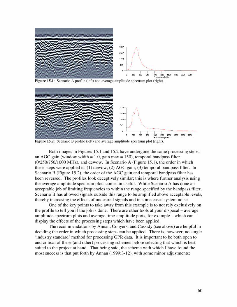
60

Figure 15.1: Scenario A profile (left) and average amplitude spectrum plot (right).

Figure 15.2: Scenario B profile (left) and average amplitude spectrum plot (right). Both images in Figures 15.1 and 15.2 have undergone the same processing steps: an AGC gain (window width = 1.0, gain max = 150), temporal bandpass filter (0/250/750/1000 MHz), and dewow. In Scenario A (Figure 15.1), the order in which these steps were applied is: (1) dewow; (2) AGC gain; (3) temporal bandpass filter. In Scenario B (Figure 15.2), the order of the AGC gain and temporal bandpass filter has been reversed. The profiles look deceptively similar; this is where further analysis using the average amplitude spectrum plots comes in useful. While Scenario A has done an acceptable job of limiting frequencies to within the range specified by the bandpass filter, Scenario B has allowed signals outside this range to be amplified above acceptable levels, thereby increasing the effects of undesired signals and in some cases system noise. One of the key points to take away from this example is to not rely exclusively on the profile to tell you if the job is done. There are other tools at your disposal – average amplitude spectrum plots and average time-amplitude plots, for example – which can display the effects of the processing steps which have been applied. The recommendations by Annan, Conyers, and Cassidy (see above) are helpful in deciding the order in which processing steps can be applied. There is, however, no single ‘industry standard’ method for processing GPR data. It is important to be both open to and critical of these (and other) processing schemes before selecting that which is best suited to the project at hand. That being said, the scheme with which I have found the most success is that put forth by Annan (1999:3-12), with some minor adjustments:

61

Step 1: Basic Data Editing – data collection parameters; line properties (type,

direction, spacing, offset, orientation, ordering); time zero correction; velocity analysis and depth conversion; static correction; rubber banding; chop, mute, merge, and stack data

Step 2: Basic Data Processing – (1) dewow; (2) gains; (3) temporal filters; (4) spatial filters

Step 3: Advanced Data Processing – 2D filters (migration and dip), deconvolution, trace attribute analysis, other operations (i.e. rectify, threshold, etc.)

Step 4: 2D Visualization – profiles (colour scale or wiggle trace; colour table; interpolation; sensitivity and contrast) and slices (colour scale; amplitude equalization; sensitivity and contrast; resolution, thickness, interpolation limit, and overlap)

Step 5: 3D Visualization – isosurfaces (isovalue; colour scale; opacity)

62

Section 3: Data Interpretation

63

Chapter 16. Uncertainty and Limitations Before any discussion of the interpretation of GPR data can be undertaken, it is first necessary to take a moment to address uncertainty and limitations. The uncertainty of any interpretation is limited by two factors: the quality of the GPR signal received (as determined by the characteristics of the propagated signal and its interaction with the subsurface – more broadly, the methodological limitations), and the quality of the comparative data by which the meaning of the signal is deduced (based on verified cases or the general principles of GPR – the interpretive limitations). Two quotes from Kvamme (2003) speak to the issues of interpretive uncertainty and methodological limitations. With respect to the former (interpretive uncertainty), Kvamme (2003:452) notes that what archaeologists often get from geophysical surveys is “numerous anomalies, but uncertainty about what they represent.” As far as acknowledgement of methodological limitations (or lack thereof), Kvamme (2003:452) notes: “archaeo-geophysicists are frequently guilty of presenting only their “best” results.” The first of these issues is the easiest to address. When discussing the anomalies detected by a GPR survey, we must be honest about our uncertainty as to what they represent. This can be easily accomplished by utilizing qualifiers (e.g., the anomaly is probably or possibly a floor) and by providing alternative explanations for the anomaly. The second issue is by far more problematic. Of course it is our first instinct to present only our best results for publication (a fault likely not limited to geophysical investigations), and further, there is always the concern of presenting ‘failures’ to the general archaeological population, ‘failures’ which may lead others to doubt our methods (again, a fault likely not limited to geophysical investigations). This will be difficult to move beyond, and I can only urge individuals to present not only their best results, but also their failures because, in the end, we have far more to learn from the great failures than the great successes. Addressing Interpretive Limitations and Uncertainty When reporting the results of any GPR survey, I recommend including a disclaimer in the report (some place where it is not likely to be skimmed over) that discusses the uncertainty and limitations of the method. This may be particularly important in cases where the purpose of the GPR survey is to identify culturally-sensitive areas that are not to be disturbed, such as human burials in archaeological and historic cemetery contexts. While the proponent of the survey should be confident in the results, he or she should also be aware that numerous factors can affect the ability of GPR to detect certain features, which may lead to both false positives and false negatives. Further, it is advisable to avoid definitive interpretations of the data, instead using such qualifiers as ‘probable’ and ‘possible’ when relating an identified anomaly to a particular archaeological feature. This is important both in cases where an imperfect GPR signal emerges in a context where a pattern in expected, and where the expected ‘perfect’ signal is present. In both cases, it is important not to rely on our expectations and aspirations. One means of curtailing any reliance on expectations and aspirations is to include alternative interpretations to any identified anomaly.

64

Below are two samples of disclaimers used in recent reports on the results of GPR surveys on the Northwest Coast of North America. The first (from Dojack 2012) hails from a survey conducted at the Stó:lō-Coast Salish settlement of Welqámex (DiRi-15), where the research questions targeted architectural features, and no culturally-sensitive features (burials) were expected to be found. The second is from a project where one of the specific purposes of GPR survey was to identify unmarked human burials in an archaeological context. The citation of this report has purposely been withheld, and all identifying markers in the text removed, to ensure the location of culturally sensitive human burials is not inadvertently disclosed to the general public. Sample Disclaimer #1 (from Dojack 2012) The results of this GPR survey can only provide locations of anomalies, which were identified based on deviations from surrounding deposits. This includes areas with distinct breaks in the stratigraphy, changes in orientation of subsurface features, some hyperbolic reflections, amplitude variations, and distinct planar reflections. It should be noted that these signals are not exclusive to archaeological features, and may represent other natural or contemporary features. Further, not all features of archaeological interest will produce a recognizable signal, in particular small-scale isolated features and those features which do not vary significantly in physical and chemical characteristics from surrounding deposits. Given methodological and interpretive limitations, most of the anomalies identified can only be given ambiguous interpretations (e.g., ‘a heterogeneous deposit of cultural or natural origins’). The use of specific archaeological terms (e.g., house floors) has been purposely limited. In most cases, anomalies can only be identified as possible features, except in those few cases where they can be verified through comparison to surface survey or subsurface excavation data. Alternative interpretations are given where appropriate, and all interpretations provided should be taken as tentative. The interpretation of anomalies relies on comparison to GPR signals collected in other contexts, in particular those that have been verified through excavation. Most of the identifications and interpretations made in this report are based on comparisons with GPR signals from other regions, given that GPR has experienced limited use thus far in investigations of household archaeology on the Northwest Coast. In addition, interpretations have been guided (and constrained) by known patterning, size, geometry, and other physical characteristics of architectural features encountered thus far in subsurface excavation at Welqámex. It is expected that this guiding knowledge does not capture the full range of variability of architectural features (or types of features) at the site, and that the imagined signals of those known features may vary from actual signals encountered in GPR images. This GPR survey is not expected to have identified all features of archaeological interest. The only means of verifying the presence and interpretation of the anomalies identified is through excavation. Comparison of future excavation results with the current GPR survey results may yield additional anomalies not initially identified, and may nullify some of the identifications and interpretations put forth in this report. Future excavations at Welqámex will be critical in refining the interpretation of GPR survey results for archaeological sites on the Northwest Coast.

65

Sample Disclaimer #2 The results of this GPR survey can only provide possible locations of human burials based on signals associated with human burials. It should be noted that these signals are not exclusive to human burials, and may represent other natural, archaeological, or contemporary features. As such, those anomalies identified can only be listed as possible human burials, and alternative interpretations are given where appropriate. Further, not all human remains will produce a recognizable signal, in particular isolated remains which are not in a formal burial context. The size of objects detected is limited by the antenna frequency (500 MHz) to objects with dimensions larger than ~15 cm. As such, this GPR survey is not expected to have identified all locations where human remains may be present. Methodological Limitations More attention has been paid to methodological limitations as compared to interpretive limitations. The feasibility of identifying particular archaeological features with GPR has been discussed by numerous researchers, including Conyers (2004:170-171), Kvamme (2008:77), and Neubauer et al (2002:136). The results of their studies are summarized in Table 16.1. The ability of GPR to detect archaeological features is related to amplitude and velocity changes at subsurface interfaces, and the size and depth of the feature. Data collection parameters can be selected to best image features of interest, and the quality of the resulting image can be further refined with post-collection processing methods.

Table 16.1: Feasibility of Using GPR to Identify Common Archaeological Features (modified from Conyers 2004:170-171; Kvamme 2008:77; Neubauer et al 2002:136)

Feature Feasibility for GPR

Pit dwellings Good Ditches, trenches, and moats Moderate to excellent House floors (soil or stone) Good to fair Compact soil or stone walls Good Cache pits Moderate Hearths/fire pits larger than 1 m diameter Good Hearths/fire pits smaller than 1 m diameter Moderate to poor Small stone tools Poor Small metal objects Moderate Large metal objects Excellent Stratigraphy thicker than radar wavelength Moderate to good Stratigraphy thinner than radar wavelength Poor Historic excavations Moderate to good Voids (incl. rodent damage) Good to excellent

66

A Note on Variability The following chapters encompass a review of a number of sources that discuss the use of GPR in archaeological contexts. The review focuses on providing descriptions of different types of anomalies encountered. It must be noted, however, that the following chapters are a review only, and present examples of certain signal types and their interpretations. These descriptions may not capture the complexities of reality, and may not encompass the full range of variability of particular archaeological features. The reader should keep Kvamme (2003:452 – “archaeo-geophysicists are frequently guilty of presenting only their “best” results”) in mind while examining the following chapters. The review also provides a preliminary list of resources which the reader can refer to for more information. This list is not exhaustive, but should provide acceptable coverage of many areas in which GPR research in archaeology has been undertaken. Many of the articles reviewed are also of methodological importance, in particular those published in the journal Archaeological Prospection. Readers with particular interest in methods should pursue these sources further.

67

Chapter 17. Signals of Burials and Tombs A number of factors will affect the ability to detect graves, tombs, and other burial-related features (discussed in depth in Doolittle and Bellantoni 2010). Doolittle and Bellantoni (2010:942, 944) make the important point that different types of burials exist, and that not only will these produce different responses, but similar responses may be produced by other objects (including roots, stones, and rodent holes). In many cases the shape, orientation, and depth of anomalies may be most useful in detecting burials (Doolittle and Bellantoni 2010:944). For the most part, the actual human remains cannot be detected (Conyers 2004:160; Conyers 2006b:70); however, there are experimental cases which suggest remains can be detected both during early and late stages of decomposition, including complete or partial skeletonisation (Schultz et al. 2006:612-614; Schultz 2008:282, 285). In these cases, the remains appear in profiles as hyperbolic anomalies (with or without distinct tails), with the remains located at its apex (Schultz et al. 2006:612-614; Schultz 2008:282; Schultz and Martin 2011:67). As such, Doolittle and Bellantoni (2010:942) recommend against migrating data when searching for graves, as hyperbolic reflections may aid in their detection. A number of secondary characteristics of burials can be used to aid in their detection. In particular, there is a marked contrast between disturbed burial shaft materials and the surrounding undisturbed deposits (Conyers 2006b:66, 70-72; Doolittle and Bellantoni 2010:946). These may appear as either low-amplitude or high-amplitude reflections in slices, and truncations or breaks in the stratigraphy in profiles (Conyers 2004:159-160; 2006b:66, 70). Burial pit edges may produce diagonal reflections (or half-hyperbolas) dipping towards one another from the upper edge of the burial feature (Goodman et al. 2009:504-505). Within the area of the grave shaft there may also occur distinct anomalies due to settling and slumping of the backfilled soil, and the accumulation of other sediments following backfilling of the grave shaft (Conyers 2006b:66, 70-72). These appear in profiles as shallow anomalies which are slightly concave-upward or bowl-shaped (Doolittle and Bellantoni 2010:946). Indeed, reference to topographic data of the survey area can be useful in identifying burial features by correlating anomalies with shifts in topography (e.g., Lorenzo and Arias 2005:528). In addition, due to the attenuation of signal strength as it passes through the remains, a low-amplitude gap may appear directly below the remains (Schultz et al. 2006:613-614). In cases where a casket, coffin, or other containment vessel is present, the burial will be more easily detected, and produce high-amplitude hyperbolic reflections, with the vessel located at the apex (Conyers 2004:161; 2006b:69-72; Conyers and Connell (2007:71); Doolittle and Bellantoni 2010:943-944). These reflections may be multiple or ringing, and may include a bright spot below the apex, which indicates an air-filled cavity (Conyers 2004:161; 2006b:69-70; Ruffell et al. 2009:389). Within the area of the containment vessel there may also occur dipping reflectors, due to multiple reflections occurring within the vessel (Hildebrand et al. 2002:19-20). Conyers (2006b:70) suggests that those hyperbolas which are narrower and lack multiple reflections are more likely to be non-metallic and/or collapsed caskets (Conyers 2006b:70). In slices, metallic vessels are visible as high-amplitude reflections, whereas non-metallic vessels produce lower-

68

amplitude signals (Conyers 2006b:70). Containment vessels are also easily identified because of their predictable sizes (Conyers 2006b:72). Cairns and other burials which are rock-covered may also appear as hyperbolas (Persson and Olofsson 2004:556), or conversely as continuous reflectors (Lorenzo and Arias 2005:529-530). Rock layers overlying burials or tombs may obscure the signal of the burial itself by producing ring-down and reverberation (Pipan et al. 2001:150). In the case of suspected burial mounds, the presence of cultural mound fill features may be key in identifying the presence (or absence) of a burial. For information on the features of cultural mounds and associated GPR anomalies, see Whittaker and Storey (2008:485-487). Research conducted by the Laboratory of Archaeology (LOA) at the University of British Columbia has used GPR to map burials in four historic cemeteries and in two mound contexts that correspond to archaeological sites containing human burials (e.g., Martindale 2009, 2010; Martindale and Daniel 2008). While the identified anomalies have not been ground-truthed, some confidence has been given to their interpretation, based on a successful blind test in which two unmarked burials interred in a different orientation to the general cemetery layout were detected and correctly interpreted without the GPR team knowing of their existence or varying orientation (Martindale 2009). GPR research by LOA has identified a pattern of burial signals which is consistent with those described above. These include the presence of high-amplitude hotspots (due to compositional differences between the burial and the surrounding matrix), transitions (between disturbed burial fill, the surrounding undisturbed stratigraphy, and the burial itself), and hyperbolic signals (present at the upper boundary of the burial). Additional patterns have been found in historic cemeteries, including consistent size (approximately 1 x 1.5-2 m for adults; child burials are smaller), orientation (burials evenly-spaced in parallel, linear rows), and depth (approximately 1-2 m below the surface). In archaeological contexts, size may vary depending on the position in which the individual was buried (dimensions of extended burials approximately 1 x 1.5-2 m, as compared to dimensions of flexed burials approximately 0.5-1 m). Burial orientation and depth may be relatively consistent in archaeological contexts, but not to the extent seen in formal cemetery contexts. A number of articles have been reviewed in compiling this report, many of which may provide helpful images and/or further sources of information. The reader is encouraged to pursue the resources relevant to his or her individual interests:

• Recent experimental and/or forensic burials: Hildebrand et al. (2002), Novo et al. (2011), Pringle et al. (2008), Schultz (2008), Schultz et al. (2006), Schultz and Martin (2011)

• Graves and cemeteries (mostly historic): Conyers (2006b), Conyers and Connell (2007), Doolittle and Bellantoni (2010), Goodman et al. (2007, 2009), Ruffell et al. (2009), Weissling (2011)

• Burial mounds and mounded tombs: Forte and Pipan (2008), Goodman et al. (2006, 2007, 2009), Kamei et al. (2000), Persson and Olofsson (2004), Pipan et al. (2001), Verdonck et al. (2009), Whittaker and Storey (2008)

69

• Chamber tombs: Böniger and Tronicke (2010), Edwards et al. (2000), Piro and Gabrielli (2009), Sarris et al. (2007)

• Megalithic tombs: Lorenzo and Arias (2005) • Mud-brick and limestone tombs: Abbas et al. (2005b) • Other potential crypts, ossuaries, and sarcophagi: Novo et al. (2010), Pérez-Gracia et al.

(2009), Ramírez-Blanco et al. (2008), Udphuay et al. (2010)

70

Chapter 18. Signals of Architectural Features In contrast to the numerous descriptions of anomaly types as they correspond to burial features, discussions of GPR imaging of architecture are comparatively loose, often dominated by talk of ‘this anomaly’ and ‘that reflection,’ which are later ‘interpreted as x feature’ with little discussion of why such an interpretation has been made. This is especially problematic in those cases where no ground-truthing or other method of evaluation has been undertaken. Granted there is a great range of architectural features and their corresponding anomalies, and laborious descriptions of each are probably beyond any researcher’s capabilities, but it is my opinion that greater effort needs to be taken among the archaeological community to define exactly what it is we think we’re seeing in GPR profiles, time slices, and isosurface maps, and justify our interpretations. It appears I am not alone in this opinion: Keay et al. (2009:155) note, with reference to geophysics in general,

“anomalies…too often are seen simply as ‘buried structures’ rather than anomalies per se. More research is needed on the ‘signatures’ of different kinds of soil, structural elements and other features, in order to better understand how they have been generated. Interpretation is equally challenging – not simply on these grounds but also because one is often constrained by interpreting structures on the basis of the degree to which they might resemble known buildings, field systems and other archaeological features”

In identifying architectural features and in particular buildings, geometric shape and patterning may be of utmost importance (e.g., Atya et al. 2005:185; Arciniega-Berard and Maillol 2008:36, Barone et al. 2011:192, Casana et al. 2008:220; Ceballos et al. 2009:1203-1204; Goodman et al. 2007:378; Weaver 2006:150). Walls and columns generally produce high amplitude reflections due to highly contrasting velocities between walls and surrounding materials (Conyers 2004:171; 2009:251); however, De La Vega et al. (2005:22) note that different types of walls produce signals of varying strength. Both columns and walls can be seen in reflection profiles as vertically stacked reflections, topped with a hyperbola (Abbas et al. 2005a:172; Barone et al. 2011:190; Conyers 2004:146; Bonomo et al. 2010:3251; Nuzzo et al. 2009:184; Yalçiner et al. 2009:1680, 1686). Walls will be imaged as linear reflectors in slice maps, which can be used to define structure extents and perimeters (Kvamme 2008:70; Ruffell et al. 2009:390). The perimeter of houses may be defined by linear high amplitude reflections in slices (see Figure 3.1) produced from house walls (Kvamme 2008:70). Floors generally produce high-amplitude, flat to slightly undulating, semi-continuous to continuous reflections, due to their large spatial extents and high velocity contrasts between the floors and surrounding materials (Conyers 2004:170-171; 2009:252; Conyers and Cameron 1998:422-423; Leucci 2002:220; Nuzzo et al. 2009:184; Yalçiner et al. 2009:1686-1687). Hearths generally produce high-amplitude reflections due to their highly reflective baked surfaces and accumulations of rocks (Conyers 2004:170; Kvamme 2008:70). They may be imaged in profiles as hyperbolic reflections (Porsani et al.

71

2010:1146-1147), or, conversely, as concave or bowl-shaped reflections (Goodman et al. 2007:381). Fire-baked kiln floors are seen to produce basin-shaped reflections (Goodman et al. 1994:319-321). Cache pits can be expected to produce similar high-amplitude reflections (Kvamme 2008:70). Pathways of movement and trails may appear in slices as areas with no significant reflection (Conyers 2010:182), or with a very strong reflection (Goodman et al. 2009:502; Weissling 2011), presumably dependant upon the construction of the footpath as compared to surrounding materials. Buried ditches and moats will be subject to focusing, producing high amplitude reflections. Conversely, convex up surfaces such as mounds, and deep narrow concave features will be subject to scattering, and are not expected to adequately resolved (Conyers 2004:73-74). Verdonck et al. (2009:198-199), however, found that a ditch with homogenous fill was characterised by few reflectors and weak low-amplitude anomalies in slices. Murdie et al. (2003:270) imaged a ditch feature as initially curved anomalies, followed by deeper irregular and discontinuous reflections. Infilled subterranean tunnels produced low-amplitude reflections (Pérez-Gracia et al. 2009; Tsokas et al. 2007). Subterranean tunnels carved from stone produce hyperbolas in profile (Lorenzo et al. 2002; Seren et al. 2008). A number of articles have been reviewed in compiling this report, many of which may provide helpful images and/or further sources of information. Individuals who are looking to learn more about GPR signals for specific architectural features are encouraged to pursue the following sources:

• Walls and columns: Abbas et al. (2005a), Appell et al. (1997), Barone et al. (2011), Berard and Maillol (2008), Bini et al. (2010), Bongiovanni et al. (2011), Booth et al. (2008), Boschi (2011), Campana et al. (2009), Casana et al. (2008), Castaldo et al. (2009), Chianese et al. (2010), Conyers (2006a, 2009, 2010, 2011), Conyers and Cameron (1998), Creasman et al. (2010), De La Vega et al. (2005), Dogan and Papamarinopoulos (2006), Goodman et al. (2009), Leckebusch (2000, 2003, 2007), Leckebusch and Peikert (2001), Leucci et al. (2007), Linford and Linford (2004), Meyer et al. (2007), Negri and Leucci (2006), Neubauer et al. (2002), Nuzzo et al. (2009), Piro et al. (2007, 2011), Trinks et al. (2010), Udphuay et al. (2010), Weaver (2006), Yalçiner et al. (2009), Zhou and Sato (2001)

• Floors and foundations: Barone et al. (2007), Berard and Maillol (2008), Boschi (2011), Castaldo et al. (2009), Conyers (1998, 2009, 2010, 2011), Conyers and Cameron (1998), Conyers and Connell (2007), Ernenwein (2006), Goodman et al. (1994, 2009), Grealy (2006), Kvamme (2008), Leckebusch (2000, 2007, 2011a), Nuzzo et al. (2009), Udphuay et al. (2010), Weaver (2006), Yalçiner et al. (2009)

• Fire pits, hearts, and kilns: Goodman et al. (1994), Kvamme (2008), Porsani et al. (2010), Rodrigues et al. (2009), Trinks et al. (2010), Weissling (2011)

• Cache pits: Kvamme (2008), Valdes and Kaplan (2000) • Postholes: Dalan et al. (2011), Trinks et al. (2010) • Pathways and roads: Castaldo et al. (2009), Conyers (2010, 2011), Conyers and

Leckebusch (2010), Goodman et al. (2009), Ernenwein and Kvamme (2008), Piro et al. (2011), Weissling (2011)

72

• Ditches, canals, and moats: Conyers (2010, 2011), Dalan et al. (2011), Goodman et al. (2009), Kamei et al. (2000), Murdie et al. (2003), Ruffell et al. (2004), Trinks et al. (2010), Verdonck et al. (2009)

• Gardens, fields, and planting beds: Conyers (2010), Conyers and Leckebusch (2010, Ernenwein and Kvamme (2008)

• Subterranean tunnels: Chávez et al. (2001), Lorenzo et al. (2002), Pérez-Gracia et al. (2009), Seren et al. (2008), Tsokas et al. (2007)

• In-filled mine shafts: Leopold and Völkel (2004) • Midden deposits: Chadwick and Madsen (2000), Conyers and Connell (2007), Rodrigues

et al. (2009), Valdes and Kaplan (2000) • Paleosols: Chapman et al. (2009).

Individuals who are looking to learn more about GPR signals for the architecture of a specific region or type are encouraged to pursue the following sources:

• Architecture in Japan: Goodman et al. (1994), Zhou and Sato (2001) • Roman, Greek, and Nabataean architecture (Mediterranean region and Europe): Appell et

al. (1997), Atya et al. (2005), Barone et al. (2007, 2011), Berard and Maillol (2008), Booth et al. (2008), Boschi (2011), Carrozzo et al. (2003), Castaldo et al. (2009), Chianese et al. (2004), Chianese et al. (2010), Conyers (2010, 2011), Conyers and Leckebusch (2010), Dogan and Papamarinopoulos (2006), Gaffney et al. (2004), Grealy (2006), Goodman et al. (2007, 2009), Kamei et al. (2002), Keay et al. (2009), Leckebusch (2007, 2011a, 2011b), Leopold et al. (2010, 2011), Leucci and Negri (2006), Linford and Linford (2004), Linford et al. (2010), Meyer et al. (2007), Negri and Leucci (2006), Neubauer et al. (2002), Nuzzo et al. (2009), Orlando (2007), Piro et al. (2003, 2007, 2011), Sarris et al. (2002), Udphuay et al. (2010), Vafidis et al. (2005), Yalçiner et al. (2009)

• Egyptian architecture: Abbas et al. (2005a, 2005b), Atya et al. (2005), Creasman et al. (2010), Kamei et al. (2002)

• Syrian tells: Casana et al. (2008) • Historic and medieval churches and castles: Bini et al. (2010), Chávez et al. (2005),

Drahor et al. (2011), Goodman et al. (2007), Leckebusch (2000), Leucci (2002, 2006), Leucci et al. (2007), Linford (2004), Novo et al. (2010), Pérez-Gracia et al. (2009), Ramírez-Blanco et al. (2008), Tsokas et al. (2007), Udphuay et al. (2010)

• Stone castles: Bini et al. (2010), Lorenzo et al. (2002), Ruffell et al. (2004), Savvaidis et al. (1999), Zhou and Sato (2001)

• Earthen and wooden architecture in Europe: Campana et al. (2009), Carey et al. (2006) Clarke et al. (1999), Goodman et al. (2009), Murdie et al. (2003), Trinks et al. (2010), Utsi (2004), Watters (2006)

• Earthen and wooden architecture in the Americas: Dalan et al. (2011), Goodman et al. (2007, 2009), Kvamme (2008), Weaver (2006)

• Puebloan architecture (American Southwest): Conyers (1998, 2006a, 2009, 2010, 2011), Conyers and Cameron (1998), Conyers and Leckebusch (2010), Ernenwein (2006), Ernenwein and Kvamme (2008), Weissling (2011)

• Architecture in South America: Bongiovanni et al. (2011), Bonomo et al. (2010), Lasaponara et al. (2011), Roosevelt (2007), Williams et al. (2007)

• Colonial/contact era architecture in the Americas: De La Vega et al. (2005), Ernenwein and Kvamme (2008), Goodman et al. (2007), Jones (2001), Pomfret (2006)

• Mesoamerican architecture: Arciniega-Ceballos et al. (2009), Chávez et al. (2001, 2009)

73

• Architecture in Hawai’i: Conyers and Connell (2007) • Coastal shell middens in the Americas: Chadwick and Madsen (2000), Rodrigues et al.

(2009), Roosevelt (2007) • Underwater architecture: Leckebusch (2003) • Subterranean settlements: Lorenzo et al. (2002), Seren et al. (2008)

74

Chapter 19. Conclusions and Future Directions Beyond Prospection GPR in archaeology is founded on its ability to act as a prospection tool for identifying potential areas of interest, where further more ‘traditional’ archaeological excavations can take place. But a current trend in the archaeological use of GPR sees a push for the shift from pure archaeological prospection to full integration with research design and use to address broader anthropological questions and theoretical issues (Conyers 2010, 2011; Conyers and Leckebusch 2010; Thompson et al. 2011). An early push for integrating archaeological geophysics into a broader anthropological theoretical framework can be seen in Kvamme (2003), where remote sensing geophysical methods are linked to landscape archaeology and questions of spatial patterning and relationships. One of the keys in this linkage is the ability of remote sensing technologies to cover significantly larger areas than ‘traditional’ excavation methods, thereby allowing investigation of more regional-oriented research questions (Kvamme 2003:453-454). Thompson et al. (2011) make further attempts to link remote sensing in archaeology to a body of theory by moving beyond Kvamme’s landscape archaeology links (noting that landscape archaeology is not a unified body of theory) and beyond the concept of place (also lacking connections to a unified body of theory). Instead, Thompson et al. (2011:197) suggest the concept of “persistent places” as a means of bridging the gap between geophysical methodology and archaeological theory. They identify four categories of questions to which remote sensing methods are most applicable: those regarding construction variation; continuities and discontinuities in the use of space; regularities in the use of space; and natural versus cultural modifications (see Thompson et al. 2011:198-210 for examples). While integrating GPR with research design and theoretical concepts are certainly admirable and achievable goals, we must remember that they may not yet be within reach for all regions. One only has to look at the preceding chapter’s list of references to see that there is an imbalance with regards to the areas in which GPR is applied. I do not think this imbalance is artificial. While GPR is an established archaeological method in some places of the world, such as the Mediterranean region and the American Southwest, where conditions are often deemed ‘ideal’ for detecting archaeological features (in particular, stone buildings in sand matrices), other regions are much farther behind in their application of GPR to archaeological investigations (for example, the Northwest Coast of North America). In these latter areas, work still needs to be done to determine the method’s applicability, refine data collection and processing techniques, and increase confidence in data interpretation. As noted by Conyers and Leckebusch (2010:68), “this type of fundamental research is common to all developing disciplines”; Thompson et al. (2011:196) echo this sentiment. In many areas of the world, GPR still falls under the category of a ‘developing discipline.’ Quantifying Uncertainty Another area of GPR in archaeology that is in need of further attention is uncertainty. As noted previously, discussions of uncertainty in interpretations of GPR data have been lax (see Chapter 16). It is worth repeating Kvamme’s (2003:452)

75

assertion that what archaeologists often get from geophysical survey is “numerous anomalies, but uncertainty about what they represent.” Unlike some archaeological methods (e.g., radiocarbon dating), the quantification of uncertainty is currently lacking in GPR analysis. Such quantification can only be derived from controlled experimentation and comparisons between GPR survey data and excavation results. In the meantime, we are left knowing that the results of GPR survey include uncertainty without a reliable means of quantifying it. In practice, most GPR analysis in archaeology focuses on the presence or absence of archaeological data, with the vast majority of studies focusing on the presence of data (remember Kvamme 2003:452 – “archaeo-geophysicists are frequently guilty of presenting only their “best” results”). The focus on the contrast between presence and absence of features obscures the issue of probability by both hiding uncertainty in the former and excluding imperfect data in the latter. The solution is to devise a probability spectrum or a multi-tiered probability scheme that eliminates the faulty presence-absence dichotomy. GPR data collected by the Laboratory of Archaeology (LOA) at the University of British Columbia may present an opportunity to empirically evaluate the GPR signal characteristics of burials. Projects conducted by LOA at a number of local First Nations cemeteries have compiled a wealth of data, some of which was collected over known burials. One could easily produce an empirically-supported probability scheme for identifying burials in local First Nations cemeteries by calculating the presence or absence of a suite of specific GPR signal characteristics (e.g., presence of high-amplitude hotspots, transitions, hyperbolas, etc.) for a sample of the data. Such a study could state with empirical certainty, for example, that in these contexts, a known percentage of burials showed clear evidence of a hyperbolic reflection in at least one reflection profile. More advanced statistics could be used to arrive at a probability scheme based on the presence or absence of a suite of GPR signal characteristics. Such a study as that outlined above would only be preliminary. Ideally, any study of uncertainty would take into account all four possible results (true positives, true negatives, false positives, and false negatives). Further, attempts should be made to address instrumental reliability and both inter-observer and intra-observer error. While it might be tempting to make efforts to estimate probability, even imprecisely and despite insufficient testing, I recommend against this approach. Applying probability estimates (in particular numerical probability estimates) is deceptive, in that they are likely to instil a false sense of confidence. This is particularly dangerous when values are applied to GPR results for studies conducted in a legal setting (or with potential to enter legal proceedings at a later date). Even if such rigorous testing is completed, the resulting probability schemes should be treated with caution. It is questionable as to whether such schemes would represent accurate generalizations that could be applied to numerous and wide-spread contexts. More likely, the resulting scheme would come with an attached disclaimer, noting that it has arisen from testing in a specific environment, and any local variations in geological or cultural deposits may render the scheme irrelevant. Further, a viable probability scheme should not be justification to override any attempts to provide alternative explanations for GPR survey results.

76

References Cited Abbas, A. M., H. Kamei, A. Helal, M. A. Atya, and F. A. Shaaban 2005a Contribution of Geophysics to Outlining the Foundation Structure of the Islamic

Museum, Cairo, Egypt. Archaeological Prospection 12:167-176. Abbas, Abbas Mohamed, Tareq Fahmy Abdallatif, Fathy A. Shaaban, Ahmed Salem, and Mancheol Suh 2005b Archaeological Investigation of the Eastern Extensions of the Karnak Temple

Using Ground-Penetrating Radar and Magnetic Tools. Geoarchaeology 20(5):537-554.

Annan, A.P. 2009 Electromagnetic Principles of Ground Penetrating Radar. In Ground Penetrating

Radar: Theory and Applications, edited by Harry M. Jol, pp. 3-40. Elsevier, Amsterdam.

1999 Practical Processing of GPR Data. Proceedings of the Second Government Workshop on Ground Penetrating Radar.

Appell, Erwin, Jörg Wilhelm, and Martin Waldhör 1997 Archaeological Prospection of Wall Remains using Geoelectrical methods and

GPR. Archaeological Prospection 4:219-229. Arciniega-Ceballos, A., E. Hernandez-Quintero, E. Cabral-Cano, L. Morett-Alatorre, O. Diaz-Molina, A. Soler-Arechalde, and R. Chavez-Segura 2009 Shallow geophysical survey at the archaeological site of San Miguel Tocuila,

Basin of Mexico. Journal of Archaeological Science 36:1199-1205. Atya, M. A., H. Kamei, A. M. Abbas, F. A. Shaaban, A. Gh. Hassaneen, M. A. Abd Alla, M. N. Soliman, Y. Marukawa, T. Ako, and Y. Kobayashi 2005 Complementary Integrated Geophysical Investigations around Al-Zayyan

Temple, Kharga Oasis, Al-Wadi Al-Jadeed (New Valley), Egypt. Archaeological

Prospection 12:177-189. Barone, P.M., F. Graziano, E. Pettinelli, and R. Ginanni Corradini 2007 Ground-penetrating Radar Investigations into the Construction Techniques of the

Cconcordia Temple (Agrigento, Sicily, Italy). Archaeological Prospection 14:47-59.

Barone, P.M., T. Bellomo, E. Mattei, S.E. Lauro, and E. Pettinelli 2011 Ground-penetrating Radar in the Regio III (Pompeii, Italy): Archaeological

Evidence. Archaeological Prospection 18:187-194. Berard, Brooke A., and J.M. Maillol 2008 Common- and Multi-Offset Ground-Penetrating Radar Study of a Roman Villa,

Tourega, Portugal. Archaeological Prospection 15:32-46.

77

Bini, Monica, Antonio Fornaciari, Adriano Ribolini, Alessandro Bianchi, Simone Sartini, and Francesco Coschino 2010 Medieval phases of settlement at Benabbio castle, Apennine mountains, Italy:

evidence from Ground Penetrating Radar survey. Journal of Archaeological

Science 37:3059-3067. Bongiovanni, María Victoria, Matías de la Vega, and Néstor Bonomo 2011 Contribution of the resistivity method to characterize mud walls in a very dry

region and comparison with GPR. Journal of Archaeological Science 38:2243-2250.

Böniger, U., and J. Tronicke 2010 Improving the interpretability of 3D GPR data using target-specific attributes:

application to tomb detection. Journal of Archaeological Science 37:672-679. Bonomo, Néstor, Ana Osella, and Norma Ratto 2010 Detecting and mapping buried buildings with Ground-Penetrating Radar at an

ancient village in northwestern Argentina. Journal of Archaeological Science 37:3247-3255.

Booth, Adam D., Neil T. Linford, Roger A. Clark, and Tavi Murray 2008 Three-dimensional, Multi-offset Ground-penetrating Radar Imaging of

Archaeological Targets. Archaeological Prospection 15:93-112. Boschi, Federica 2011 Geophysical Survey of the Burnum Archaeological Site, Croatia. Archaeological

Prospection 18:117-126. Campana, S., M. Dabas, L. Marasco, S. Piro, and D. Zamuner 2009 Integration of Remote Sensing, Geophysical Surveys and Archaeological

Excavation for the Study Of A Medieval Mound (Tuscany, Italy). Archaeological

Prospection 16:167-176. Carey, Chris J., Tony G. Brown, Keith C. Challis, Andy J. Howard, and Lynden Cooper 2006 Predictive Modelling of Multiperiod Geoarchaeological Resources at a River

Confluence: a Case Study from the Trent-Soar, UK. Archaeological Prospection 13:241-250.

Carrozzo, M. T., G. Leucci, S. Negri, and L. Nuzzo 2003 GPR Survey to Understand the Stratigraphy of the Roman Ships Archaeological

Site (Pisa, Italy). Archaeological Prospection 10:57-72. Casana, Jesse, Jason T. Herrmann, and Aaron Fogel 2008 Deep Subsurface Geophysical Prospection at Tell Qarqur, Syria. Archaeological

Prospection 15:207-225.

78

Cassidy, Nigel J. 2009a Ground Penetrating Radar Data Processing, Modelling and Analysis. In Ground

Penetrating Radar: Theory and Applications, edited by Harry M. Jol, pp. 141-176. Elsevier, Amsterdam.

2009b Electrical and Magnetic Properties of Rocks, Soils and Fluids. In Ground

Penetrating Radar: Theory and Applications, edited by Harry M. Jol, pp. 41-72. Elsevier, Amsterdam.

Castaldo, R., L. Crocco, M. Fedi, B. Garofalo, R. Persico, A. Rossi, and F. Soldovieri 2009 GPR Microwave Tomography for Diagnostic Analysis of Archaeological Sites:

the Case of a Highway Construction in Pontecagnano (Southern Italy). Archaeological Prospection 16:203-217.

Chadwick, William J., and John A. Madsen 2000 The Application of Ground-penetrating Radar to a Coastal Prehistoric

Archaeological Site, Cape Henlopen, Delaware, USA. Geoarchaeology 15(8):765-781.

Chapman, Henry, Jimmy Adcock, and John Gater 2009 An approach to mapping buried prehistoric palaeosols of the Atlantic seaboard in

Northwest Europe using GPR, geoarchaeology and GIS and the implications for heritage management. Journal of Archaeological Science 36:2308-2313.

Chávez, R. E., M. E. Cámara, A. Tejero, L. Barba, and L. Manzanilla 2001 Site Characterization by Geophysical Methods in The Archaeological Zone of

Teotihuacan, Mexico. Journal of Archaeological Science 28:1265-1276. Chávez, René Efrain, Maria Encarnación Cámara, Rocio Ponce, and Denisse Argote 2005 Use of Geophysical Methods in Urban Archaeological Prospection: The Basilica

de Neustra Señora de La Salud, Patzcuaro, Mexico. Geoarchaeology 20(5):505-519.

Chávez, R. E., A. Tejero, D. L. Argote, and M. E. Cámara 2009 Geophysical Study of a Pre-Hispanic Lakeshore Settlement, Chiconahuapan Lake,

Mexico. Archaeological Prospection 17:1-13. Chianese, D., V. Lapenna, S. Di Salvia, A. Perrone, and E. Rizzo 2010 Joint geophysical measurements to investigate the Rossano of Vaglio

archaeological site (Basilicata Region, Southern Italy). Journal of Archaeological

Science 37:2237-2244. Chianese, Domenico, Mariagrazia D’Emilio, Saverio Di Salvia, Vincenzo Lapenna, Maria Ragosta, and Enzo Rizzo 2004 Magnetic mapping, ground penetrating radar surveys and magnetic susceptibility

measurements for the study of the archaeological site of Serra di Vaglio (southern Italy). Journal of Archaeological Science 31:633-643.

79

Clarke, Ciara M., Erica Utsi, and Vincent Utsi 1999 Ground Penetrating Radar Investigations at North Ballachulish Moss, Highland,

Scotland. Archaeological Prospection 6:107-121. Conyers, Lawrence B. 2011 Discovery, mapping and interpretation of buried cultural resources non-invasively

with ground-penetrating radar. Journal of Geophysics and Engineering 8:S13-S22.

2010 Ground-penetrating radar for anthropological research. Antiquity 84:175-184. 2009 Ground-penetrating radar for landscape archaeology: Method and applications. In

Seeing the Unseen, edited by Stefano Campana and Salvatore Piro, pp. 245-255. Taylor and Francis Group, London.

2007 Ground-penetrating Radar for Archaeological Mapping. In Remote Sensing in

Archaeology, edited by James Wiseman and Farouk El-Baz, pp. 329-344. Springer, New York.

2006a Innovative Ground-penetrating Radar Methods for Archaeological Mapping. Archaeological Prospection 13:139-141.

2006b Ground-Penetrating Radar Techniques to Discover and Map Historic Graves. Historical Archaeology 40(3):64-73.

2004 Ground-Penetrating Radar for Archaeology. AltaMira Press, Lanham. 1998 Acquisition, Processing and Interpretation Techniques for Ground-Penetrating

Radar Mapping of Buried Pit-Structures in the American Southwest. In Proceedings of the 5

th International Conference on Ground-penetrating Radar,

pp. 89-94. Tohoku University Faculty of Engineering, Sendai, Japan. Conyers, Lawrence B., and Catherine M. Cameron 1998 Ground-Penetrating Radar Techniques and Three-Dimensional Computer

Mapping in the American Southwest. Journal of Field Archaeology 25(4):417-430.

Conyers, Lawrence B., and Samuel Connell 2007 An Analysis of Ground-Penetrating Radar’s Ability to Discover and Map Buried

Archaeological Sites in Hawai’i. Hawaiian Archaeology Journal 11:62-77. Conyers, Lawrence B., and Juerg Leckebusch 2010 Geophysical Archaeology Research Agendas for the Future: Some Ground-

penetrating Radar Examples. Archaeological Prospection 17(2):117-123. Creasman, Pearce Paul, Douglas Sassen, Samuel Koepnick, and Noreen Doyle 2010 Ground-penetrating radar survey at the pyramid complex of Senwosret III at

Dahshur, Egypt, 2008: search for the lost boat of a Pharaoh. Journal of

Archaeological Science 37:516-524.

80

Dalan, Rinita A., Bruce W. Bevan, Dean Goodman, Dan Lynch, Steven de Vore, Steve Adamek, Travis Martin, George Holley, and Michael Michlovic 2011 The Measurement and Analysis of Depth in Archaeological Geophysics: Tests at

the Biesterfeldt Site, USA. Archaeological Prospection 18:245-265. Daniel, Steve nd Ground Penetrating Radar Data Collection: A Field Guide to Project Planning and

Execution. Unpublished report, to be posted online at UBC’s digital repository (cIRcle - https://circle.ubc.ca/).

De La Vega, M., A. Osella, E. Lascano, and J.M. Carcione 2005 Ground-penetrating Radar and Geoelectrical Simulations of Data from the

Floridablanca Archaeological Site. Archaeological Prospection 12:19-30. Dogan, M., and S. Papamarinopoulos 2006 Exploration of the Hellenistic Fortification Complex at Asea Using a

Multigeophysical Prospection Approach. Archaeological Prospection 13:1-9. Dojack, Lisa 2012 Report on the 2010-2011 Ground Penetrating Radar Survey at Welqamex (DiRi-

15), Hope, Southwestern B.C. Unpublished report on file at Stó:lō Research & Resource Management Centre, Chilliwack, BC.

Doolittle, James A., and Nicholas F. Bellantoni 2010 The search for graves with ground-penetrating radar in Connecticut. Journal of

Archaeological Science 37:941-949. Drahor, Mahmut G., Meriç A. Berge, and Caner Öztürk 2011 Integrated geophysical surveys for the subsurface mapping of buried structures

under and surrounding of the Agios Voukolos Church in İzmir, Turkey. Journal

of Archaeological Science 38:2231-2242. Edwards, Walter, Masaaki Okita, and Dean Goodman 2000 Investigation of a Subterranean Tomb in Miyazaki, Japan. Archaeological

Prospection 7:215-224. Ernenwein, Eileen G. 2006 Imaging in the Ground-penetrating Radar Near-field Zone: a Case Study from

New Mexico, USA. Archaeological Prospection 13:154-156. Ernenwein, Eileen G., and Kenneth L. Kvamme 2008 Data Processing Issues in Large-area GPR Surveys: Correcting Trace

Misalignments, Edge Discontinuities and Striping. Archaeological Prospection

15:133-149.

81

Forte, E., and M. Pipan 2008 Integrated seismic tomography and ground-penetrating radar (GPR) for the high-

resolution study of burial mounds (tumuli). Journal of Archaeological Science

35:2614-2623. Gaffney, V., H. Patterson, S. Piro, D. Goodman, and Y. Nishimura 2004 Multimethodological Approach to Study and Characterize Forum Novum

(Vescovio, Central Italy). Archaeological Prospection 11:201-212. Golden Software 2006 Voxler Getting Started Guide: 3D Data Visualization. Golden Software, Inc. Goodman, Dean, Yasushi Nishimura, Hiromichi Hongo, and Noriaki Higashi 2006 Correcting for Topography and the Tilt of Ground-penetrating Radar Antennae.

Archaeological Prospection 13:157-161. Goodman, D., Y. Nishimura, T. Uno, and T. Yamamoto 1994 A Ground Radar Survey of Medieval Kiln Sites in Suzu City, Western Japan.

Archaeometry 36(2):317-326. Goodman, Dean, Salvatore Piro, Yasushi Nishimura, Kent Schneider, Hiromichi Hongo, Noriaki Higashi, John Steinberg, and Brian Damiata 2009 GPR Archaeometry. In Ground Penetrating Radar: Theory and Applications,

edited by Harry M. Jol, pp. 479-508. Elsevier, Amsterdam. Goodman, Dean, Kent Schneider, Salvatore Piro, Yasushi Nishimura, and Agamemnon G. Pantel 2007 Ground Penetrating Radar Advances in Subsurface Imaging for Archaeology. In

Remote Sensing in Archaeology, edited by James Wiseman and Farouk El-Baz, pp. 375-394. Springer, New York.

Grealy, Michael 2006 Resolution of Ground-penetrating Radar Reflections at Differing Frequencies.

Archaeological Prospection 13:142-146. Hildebrand, J. A., S. M. Wiggins, P. C. Henkart, and L. B. Conyers 2002 Comparison of Seismic Reflection and Ground-penetrating Radar Imaging at the

Controlled Archaeological Test Site, Champagin, Illinois. Archaeological

Prospection 9:9-21. Jones, Geoffrey 2001 Geophysical Investigation at the Falling Creek Ironworks, an Early Industrial Site

in Virginia. Archaeological Prospection 8:247-256.

82

Kamei, Hiroyuki, Magdy Ahmed Atya, Tareq Fahmy Abdallatif, Masato Mori, and Pasomphone Hemthavy 2002 Ground-penetrating Radar and Magnetic Survey to the West of Al-Zayyan

Temple, Kharga Oasis, Al-Wadi Al-Jadeed (New Valley), Egypt. Archaeological

Prospection 9:93-104. Kamei, Hiroyuki, Yuzo Marukawa, Hiroshi Kudo, Yasushi Nishimura, and Masayuki Nakai 2000 Geophysical Survey of Hirui-Otsuka Mounded Tomb in Ogaki, Japan.

Archaeological Prospection 7:225-230. Keay, Simon, Graeme Earl, Sophie Hay, Stephen Kay, Jessica Ogden, and Kristian D. Strutt 2009 The Role of Integrated Geophysical Survey Methods in the Assessment of

Archaeological Landscapes: the Case of Portus. Archaeological Prospection

16:154-166. Kvamme, Kenneth L. 2008 Archaeological Prospecting at the Double Ditch State Historic Site, North Dakota,

USA. Archaeological Prospection 15:62-79. 2003 Geophysical Surveys as Landscape Archaeology. American Antiquity 68(3):435-

457. Lasaponara, Rosa, Nicola Masini, Enzo Rizzo, and Giuseppe Orefici 2011 New discoveries in the Piramide Naranjada in Cahuachi (Peru) using satellite,

Ground Probing Radar and magnetic investigations. Journal of Archaeological

Science 38:2031-2039. Leckebusch, Jürg 2011a Problems and Solutions with GPR Data Interpretation: Depolarization and Data

Continuity. Archaeological Prospection 18:303-308. 2011b Comparison of a Stepped-Frequency Continuous Wave and a Pulsed GPR

System. Archaeological Prospection 18:15-25. 2007 Pull-up/Pull-down Corrections for Ground-penetrating Radar Data.

Archaeological Prospection 14:142-145. 2003 Ground-penetrating Radar: A Modern Three-dimensional Prospection Method.

Archaeological Prospection 10:213-240. 2000 Two- and Three-dimensional Ground-penetrating Radar Surveys Across a

Medieval Choir: a Case Study in Archaeology. Archaeological Prospection

7:189-200. Leckebusch, Jürg, and Ronald Peikert 2001 Investigating the True Resolution and Three-dimensional Capabilities of Ground-

penetrating Radar Data in Archaeological Surveys: Measurements in a Sand Box. Archaeological Prospection 8:29-40.

83

Leopold, Matthias, and Jörg Völkel 2004 Neolithic Flint Mines in Arnhofen, Southern Germany: A Ground-penetrating

Radar Survey. Archaeological Prospection 11:57-64. Leopold, Matthias, Thomas Plöckl, Gunter Forstenaicher, and Jörg Völkel 2010 Integrating pedological and geophysical methods to enhance the informative

value of an archaeological prospection – The example of a Roman villa rustica

near Regensburg, Germany. Journal of Archaeological Science 37:1731-1741. Leopold, Matthias, Evey Gannaway, Jörg Völkel, Florian Haas, Michael Becht, Tobias Heckmann, Markus Westphal, and Gerhard Zimmer 2011 Geophysical Prospection of a Bronze Foundry on the Southern Slope of the

Acropolis at Athens, Greece. Archaeological Prospection 18:27-41. Leucci, Giovanni 2006 Contribution of Ground Penetrating Radar and Electrical Resistivity Tomography

to identify the cavity and fractures under the main Church in Botrugno (Lecce, Italy). Journal of Archaeological Science 33:1194-1204.

2002 Ground-penetrating Radar Survey to Map the Location of Buried Structures under Two Churches. Archaeological Prospection 9:217-228.

Leucci, Giovanni, and Sergio Negri 2006 Use of ground penetrating radar to map subsurface archaeological features in an

urban area. Journal of Archaeological Science 33:502-512. Leucci, Giovanni, Rosella Cataldo, and Giorgio De Nunzio 2007 Assessment of fractures in some columns inside the crypt of the Cattedrale di

Otranto using integrated geophysical methods. Journal of Archaeological Science

34:222-232. Linford, Neil 2004 From Hypocaust to Hyperbola: Ground-penetrating Radar Surveys over mainly

Roman Remains in the UK. Archaeological Prospection 11:237-246. Linford, N. T., and P. K. Linford 2004 Ground Penetrating Radar Survey over a Roman Building at Groundwell Ridge,

Blunsdon St Andrew, Swindon, UK. Archaeological Prospection 11:49-55. Linford, Neil, Paul Linford, Louise Martin, and Andy Payne 2010 Stepped Frequency Ground-penetrating Radar Survey with a Multi-element Array

Antenna: Results from Field Application on Archaeological Sites. Archaeological

Prospection 17:187-198.

84

Lorenzo, Henrique, and Pedro Arias 2005 A Methodology for Rapid Archaeological Site Documentation Using Ground-

Penetrating Radar and Terrestrial Photogrammetry. Geoarchaeology 20(5):521-535.

Lorenzo, H., M. C. Hernández, and V. Cuéllar 2002 Selected Radar Images of Man-made Underground Galleries. Archaeological

Prospection 9:1-7. Martindale, Andrew 2010 2009 Musqueam-UBC Field School – ANTH 306 Final Report submitted to the

Musqueam Indian Band and UBC Laboratory of Archaeology. 2009 2008 Musqueam-UBC Field School – ANTH 306 Final Report submitted to the

Musqueam Indian Band and UBC Laboratory of Archaeology. Martindale, Andrew, and Steve Daniel 2008 2007 Musqueam-UBC Field School – ANTH 306 Final Report submitted to the

Musqueam Indian Band and UBC Laboratory of Archaeology. Meyer, Cornelius, Burkart Ullrich, and Christophe D.M. Barlieb 2007 Archaeological Questions and Geophysical Solutions: Ground-Penetrating Radar

and Induced Polarization Investigations in Munigua, Spain. Archaeological

Prospection 14:202-212. Murdie, R. E., N. R. Goulty, R. H. White, G. Barratt, N. J. Cassidy, and V. Gaffney 2003 Comparison of Geophysical Techniques for Investigating an Infilled Ditch at

Bury Walls Hill Fort, Shropshire. Archaeological Prospection 10:265-276. Negri, Sergio, and Giovanni Leucci 2006 Geophysical investigation of the Temple of Apollo (Hierapolis, Turkey). Journal

of Archaeological Science 33:1505-1513. Neubauer, W., A. Eder-Hinterleitner, S. Seren, and P. Melichar 2002 Georadar in the Roman Civil Town Carnuntum, Austria: An Approach for

Archaeological Interpretation of GPR Data. Archaeological Prospection 9:135-156.

Novo, Alexandre, Henrique Lorenzo, Fernando I. Rial, and Mercedes Solla 2011 3D GPR in forensics: Finding a clandestine grave in a mountainous environment.

Forensic Science International 204:134-138. 2010 Three-dimensional Ground-penetrating radar Strategies over an Indoor

Archaeological Site: Convent of Santo Domingo (Lugo, Spain). Archaeological

Prospection 17:213-222.

85

Nuzzo, Luigia, Giovanni Leucci, and Sergio Negri 2009 GPR, ERT and Magnetic Investigations Inside the Martyrium of St Philip,

Hierapolis, Turkey. Archaeological Prospection 16:177-192. Orlando, Luciana 2007 Georadar Data Collection, Anomaly Shape and Archaeological Interpretation – a

Case Study from Central Italy. Archaeological Prospection 14:213-225. Pérez-Gracia, V., J.O. Caselles, J. Clapes, R. Osorio, G. Martínez, and J.A. Canas 2009 Integrated near-surface geophysical survey of the Cathedral of Mallorca. Journal

of Archaeological Science 36:1289-1299. Persson, Kjell, and Bo Olofsson 2004 Inside a mound: Applied geophysics in archaeological prospecting at the Kings’

Mounds, Gamla Uppsala, Sweden. Journal of Archaeological Science 31:551-562.

Pipan, M., L. Baradello, E. Forte, and I. Finetti 2001 Ground Penetrating Radar Study of Iron Age Toms in Southeastern Kazakhstan.

Archaeological Prospection 8:141-155. Piro, Salvatore, and Roberto Gabrielli 2009 Multimethodological Approach to Investigate Chamber Tombs in the Sabine

Necropolis at Colle del Forno (CNR, Rome, Italy). Archaeological Prospection

16:111-124. Piro, S., D. Goodman, and Y. Nishimura 2003 The Study and Characterization of Emperor Traiano’s Villa (Altopiani di

Arcinazzo, Roma) using High-resolution Integrated Geophysical Surveys. Archaeological Prospection 10:1-25.

Piro, S., D. Peloso, and R. Gabrielli 2007 Integrated Geophysical and Topographical Investigation in the Territory of

Ancient Tarquinia (Viterbo, Central Italy). Archaeological Prospection 14:191-201.

Piro, S., G. Ceraudo, and D. Zamuner 2011 Integrated Geophysical and Archaeological Investigations of Aquinum in

Frosinone, Italy. Archaeological Prospection 18:127-138. Pomfret, James 2006 Ground-penetrating Radar Profile Spacing and Orientation for Subsurface

Resolution of Linear Features. Archaeological Prospection 13:151-152.

86

Porsani, Jorge Luís, Guilherme de Matos Jangelme, and Renato Kipnis 2010 GPR survey at Lapa do Santo archaeological site, Lagoa Santa karstic region,

Minas Gerais state, Brazil. Journal of Archaeological Science 37:1141-1148. Pringle, Jamie K., John Jervis, John P. Cassella, and Nigel J. Cassidy 2008 Time-Lapse Geophysical Investigations over a Simulated Urban Clandestine

Grave. Journal of Forensic Science 53(6):1405-1416. Ramírez-Blanco, Manuel, Francisco García-García, Isabel Rodríguez-Abad, Rosa Martínez-Sala, and Javier Benlloch 2008 Ground-Penetrating Radar Survey for Subfloor Mapping and Analysis of

Structural Damage in the Sagrado Corazón de Jesús Church, Spain. Archaeological Prospection 15:285-292.

Rodrigues, Selma I., Jorge L. Porsani, Vinicius R.N. Santos, Paulo A.D. DeBlasis, and Paulo C.F. Giannini 2009 GPR and inductive electromagnetic surveys applied in three coastal sambaqui

(shell mounds) archaeological sites in Santa Catarina state, South Brazil. Journal

of Archaeological Science 36:2081-2088. Roosevelt, A.C. 2007 Geophysical Archaeology in the Lower Amazon: A Research Strategy. In Remote

Sensing in Archaeology, edited by James Wiseman and Farouk El-Baz, pp. 443-475. Springer, New York.

Ruffell, Alastair, Lousie Geraghty, Colin Brown, and Kevin Barton 2004 Ground-penetrating Radar Facies as an aid to Sequence Stratigraphic Analysis:

Application to the Archaeology of Clonmacnoise Castle, Ireland. Archaeological

Prospection 11:247-262. Ruffell, Alastai, Alan McCabe, Colm Donnelly, and Brian Sloan 2009 Location and Assessment of an Historic (150-160 Years Old) Mass Grave Using

Geographic and Ground Penetrating Radar Investigation, NW Ireland. Journal of

Forensic Sciences 54(2):382-394. Sarris, A., E. Athanassopoulou, A. Doulgeri-Intzessiloglou, Eu. Skafida, and J. Weymouth 2002 Geological Prospection Survey of an Ancient Amphorae Workshop at Tsoukalia,

Alonnisos (Greece). Archaeological Prospection 9:183-195. Sarris, A., R.K. Dunn, J.L. Rife, N. Papadopoulos, E. Kokkinou, and C. Mundigler 2007 Geological and Geophysical Investigations in the Roman Cemetery at Kenchreai

(Korinthia), Greece. Archaeological Prospection 14:1-23.

87

Savvaidis, A., G. Tsokas, Y. Liritzis, and M. Apostolou 1999 The Location and Mapping of Ancient Ruins on the Castle of Lefkas (Greece) by

Resistivity and GPR Methods. Archaeological Prospection 6:63-73. Schultz, John J. 2008 Sequential Monitoring of Burials Containing Small Pig Cadavers Using Ground

Penetrating Radar. Journal of Forensic Sciences 53(2):279-287. Schultz, John J., Mary E. Collins, and Anthony B. Falsetti 2006 Sequential Monitoring of Burials Containing Large Pig Cadavers Using Ground-

Penetrating Radar. Journal of Forensic Sciences 51(3):607-616. Schultz, John J., and Michael M. Martin 2011 Controlled GPR grave research: Comparison of reflection profiles between 500

and 250 MHz antennae. Forensic Science International 209:64-69. Sensors & Software 2007a EKKO_Mapper User’s Guide. Sensors & Software, Mississauga. 2007b GFP_View & GFP_Edit User’s Guide. Sensors & Software, Mississauga. 2003 EKKO_View Enhanced & EKKO_View Deluxe User’s Guide. Sensors &

Software, Mississauga. 1999a Ground Penetrating Radar Survey Design. Sensors & Software, Mississauga. 1999b Velocity Analysis. Sensors & Software, Mississauga. Seren, Aysel, Kenan Gelisli, and Aycan Catakli 2008 A Geophysical Investigation of the Late Roman Underground Settlement at

Aydintepe, Northeast Turkey. Geoarchaeology 23(6):842-860. Thompson, Victor D., Philip J. Arnold III, Thomas J. Pluckhahn, and Amber M. Vanderwarker 2011 Situating Remote Sensing in Anthropological Archaeology. Archaeological

Prospection 18:195-213. Trinks, Immo, Bernth Johansson, Jaana Gustafsson, Jesper Emilsson, Johan Friborg, Christer Gustafsson, Johan Nissen, and Alois Hinterleitner 2010 Efficient, Large-scale Archaeological Prospection using a True Three-

dimensional Ground-penetrating Radar Array System. Archaeological

Prospection 17:175-186. Tsokas, G. N., A. Stampolidis, I. Mertzanidis, P. Tsourlos, R. Hamza, C. Chrisafis, D. Ambonis, and I. Tavlakis 2007 Geophysical Exploration in the Church of Protaton at Karyes of Mount Athos

(Holy Mountain) in Northern Greece. Archaeological Prospection 14:75-86.

88

Udphuay, Suwimon, Vivian L. Paul, Mark E. Everett, and Robert B. Warden 2010 Ground-penetrating Radar Imaging of Twelfth Century Romanesque Foundations

Beneath the Thirteenth Century Gothic Abbey Church of Valmagne, France. Archaeological Prospection 17:199-212.

Utsi, Erica 2004 Ground-penetrating Radar Time-slices from North Ballachulish Moss.

Archaeological Prospection 11:65-75. Vafidis, A., N. Economou, Y. Ganiatsos, M. Manakou, G. Poulioudis, G. Sourlas, E. Vrontaki, A. Sarris, M. Guy, and Th. Kalpaxis 2005 Integrated geophysical studies at ancient Itanos (Greece). Journal of

Archaeological Science 32:1023-1036. Valdes, Juan Antonio, and Jonathan Kaplan 2000 Ground-Penetrating Radar at the Maya Site of Kaminaljuyu, Guatemala. Journal

of Field Archaeology 27(3):329-342. Verdonck, L., D. Simpson, W.M. Cornelis, A. Plyson, J. Bourgeois, R. Docter, and M. Van Meirvenne 2009 Ground-penetrating Radar Survey over Bronze Age Circular Monuments on a

Sandy Soil, Complemented with Electromagnetic Induction and Fluxgate Gradiometer Data. Archaeological Prospection 16:193-202.

Watters, Margaret S. 2006 Geovisualization: an Example from the Catholme Ceremonial Complex.

Archaeological Prospection 13:282-290. Weaver, Wendy 2006 Ground-penetrating Radar Mapping in Clay: Success from South Carolina, USA.

Archaeological Prospection 13:147-150. Weissling, Blake P. 2011 Historical Tracks and Trail Resources as Delineated by Near-field Ground-

penetrating Radar: Two Case Studies. Archaeological Prospection 2011:1-6. Whittaker, William E., and Glenn R. Storey 2008 Ground-Penetrating Radar Survey of the Sny Magill Mound Group, Effigy

Mounds National Monument, Iowa. Geoarchaeology 23(4):474-499. Williams, Patrick Ryan, Nicole Couture, and Deborah Blom 2007 Urban Structure at Tiwanaku: Geophysical Investigations in the Andean

Altiplano. In Remote Sensing in Archaeology, edited by James Wiseman and Farouk El-Baz, pp. 423-441. Springer, New York.

89

Yalçiner, C. Ç., M. Bano, M. Kadioglu, V. Karabacak, M. Meghraoui, and E. Altunel 2009 New temple discovery at the archaeological site of Nysa (western Turkey) using

GPR method. Journal of Archaeological Science 36:1680-1689. Zhou, Hui, and Motoyuki Sato 2001 Archaeological Investigation in Sendai Castle using Ground-Penetrating Radar.

Archaeological Prospection 8:1-11.