business forecasting - teeportal.tee.gr/.../seminaria/.../metrhsh_apodoshs/methodoi_provle… ·...
TRANSCRIPT

Business ForecastingBusiness Forecasting in Real Problemsin Real Problems
Dr Dimitrios AidonisDr. Dimitrios AidonisLecturer
Department of Logistics
f h l ikiATEI of Thessaloniki

ForecastingForecastingForecastingForecasting
• The use of forecasting is wide and it has a long history
• Ancient years (Delfi, Incas)y ( , )
• Astrology, Future Tellers
l h• Sciences: e.g. Metereology, Physics
• Finance: e.g. Stock Market
• In Real Life: Economic Crisis
PredictionPrediction isis veryvery difficult,difficult, especiallyespecially ifif itit isis aboutabout thethe FUTUREFUTURE
Niels Bohr Received Nobel Prize in Physics (1922)Niels Bohr, Received Nobel Prize in Physics (1922)
SINTROME 2012 –Simulation Training in Operations Management 22

Business Fields of Interest Business Fields of Interest Business Fields of Interest Business Fields of Interest
In business, forecasting can be used in all management levels.
Crucial role in scheduling raw materials, human resources, operationsg , , p
etc.
/ fAccounting : Cost / profit estimates
Finance: Funding and cash flows
Marketing: Promotion strategy, pricing strategy
Operations: Schedules workloadsOperations: Schedules, workloads
Human Resources (HR): Training needs, location of resources,
hiring recruiting needs
Research and Development: New product/service designResearch and Development: New product/service design
SINTROME 2012 –Simulation Training in Operations Management 33

The Role of ForecastingThe Role of ForecastingThe Role of ForecastingThe Role of Forecasting
FORECASTING for Maximizing System’s Effectiveness
SINTROME 2012 –Simulation Training in Operations Management 44

Forecast Characteristics Forecast Characteristics (1/3)(1/3)Forecast Characteristics Forecast Characteristics (1/3)(1/3)
Forecasts are not usually wrong, they are ALWAYS WRONG!!!
• Flexibility is the only solution to this problemy y p
A good forecast is usually more than a single number
f l ( )• Extra information is given, e.g. error, value range (40±5 items)
The longer the forecasting horizon, the less accurate the forecasts
will be
• Is it safer to forecast the demand of products for tomorrow or• Is it safer to forecast the demand of products for tomorrow or
for the same day after one year?
• The answer is simple: FOR TOMORROW
SINTROME 2012 –Simulation Training in Operations Management 55

Forecast Characteristics Forecast Characteristics (2/3)(2/3)Forecast Characteristics Forecast Characteristics (2/3)(2/3)
Aggregate forecasts are more accurate (more products)
Product Α: AD=5, F=4, E= 1/5 (20%), , ( )
Product Β: AD=5, F=5, E= 0 /0 (0%)
d / ( %)Product C: AD=5, F=4, E= 1 /5 (20%)
Product D: AD=5, F=6, E= ‐1/5 (20%)
where AD: Actual Demand, F: Forecast and E: Error
Total AD=20 F=19 E=1/20 (5%)
66SINTROME 2012 –Simulation Training in Operations Management 66

The 6 Elements of Precise ForecastingThe 6 Elements of Precise ForecastingThe 6 Elements of Precise ForecastingThe 6 Elements of Precise Forecasting
Should be TIMELY
Should be ACCURATE
Should be RELIABLE
Should be in MEANINGFUL
UNITS
Should be presented in WRITTING
Should be EASE TO USEUNITS WRITTING EASE TO USE
77SINTROME 2012 –Simulation Training in Operations Management 77

Forecasting Horizon Forecasting Horizon (1/3)(1/3)Forecasting Horizon Forecasting Horizon (1/3)(1/3)
Short term (days or weeks)( y )
• Inventory management
d• Orders execution
• Production and material planning (MRP)
• Work shifts
Operational Level
SINTROME 2012 –Simulation Training in Operations Management 88

Forecasting Horizon Forecasting Horizon (2/3)(2/3)Forecasting Horizon Forecasting Horizon (2/3)(2/3)
Intermediate term (weeks or months)( )
• Inventory levels
l f d f l• Sales patterns for product families
• Requirements and abilities of employees
• Resources requirements
Tactical level
99SINTROME 2012 –Simulation Training in Operations Management 99

Forecasting Horizon Forecasting Horizon (3/3)(3/3)Forecasting Horizon Forecasting Horizon (3/3)(3/3)
Long term (months or years)g ( y )
• Long term planning of capacity needs
d h l• Needs in new technologies
• Search for new markets
• Search for new alliances
Strategic level
SINTROME 2012 –Simulation Training in Operations Management 1010

Forecast SystemsForecast Systems (1/3)(1/3)Forecast SystemsForecast Systems (1/3)(1/3)
ForecastForecast SystemSystem:: a number of methods and techniques employed for
collecting, processing and analyzing input data in order to come up with
the right conclusions (output data)
1111SINTROME 2012 –Simulation Training in Operations Management 1111

Forecast SystemsForecast Systems (2/3)(2/3)Forecast SystemsForecast Systems (2/3)(2/3)
InputInput DataData
InternalInternal SourcesSources ofof InformationInformation::
• Historic data (e.g. demand of raw materials, sales).
• Executive opinionsExecutive opinions
• Market surveys
ExternalExternal SourcesSources ofof InformationInformation::
• Consulting firms
• Research institutes
• Public bodies
1212SINTROME 2012 –Simulation Training in Operations Management 1212
Forecast SystemsForecast Systems (3/3)(3/3)Forecast SystemsForecast Systems (3/3)(3/3)
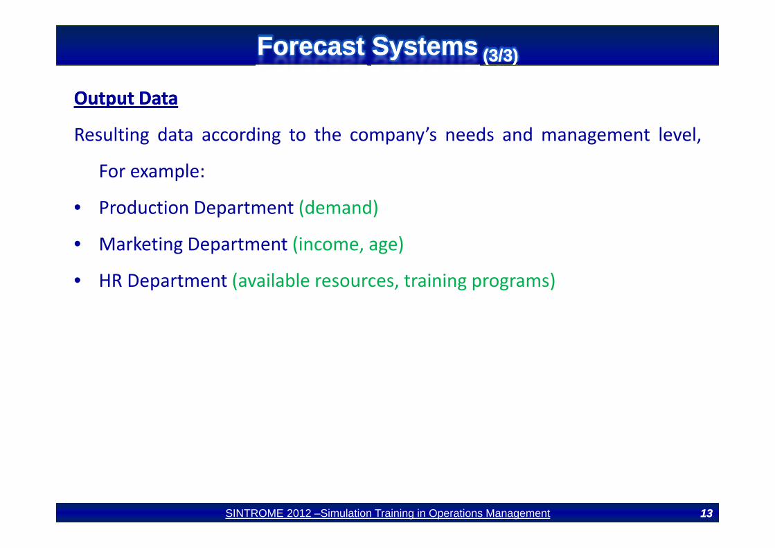
OutputOutput DataData
Resulting data according to the company’s needs and management level,
For example:
• Production Department (demand)Production Department (demand)
• Marketing Department (income, age)
HR D ( il bl i i )• HR Department (available resources, training programs)
1313SINTROME 2012 –Simulation Training in Operations Management 1313

Forecasting MethodsForecasting MethodsForecasting MethodsForecasting Methods
Qualitative Methods (relied on opinion and intuition)
• Jury of executive opinion
• Sales force composite
• Consumer surveys
• The Delphi method
Quantitative methods (use of mathematical models and historical
data)
• Casual methods
• Time series methods
1414SINTROME 2012 –Simulation Training in Operations Management 1414
Qualitative MethodsQualitative Methods (1/3)(1/3)Qualitative MethodsQualitative Methods (1/3)(1/3)
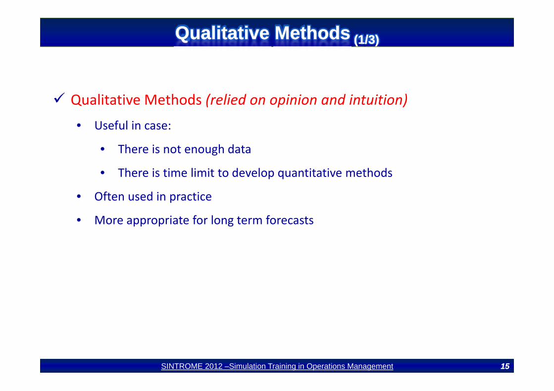
Qualitative Methods (relied on opinion and intuition)( p )
• Useful in case:
• There is not enough dataThere is not enough data
• There is time limit to develop quantitative methods
• Often used in practice• Often used in practice
• More appropriate for long term forecasts
1515SINTROME 2012 –Simulation Training in Operations Management 1515

Qualitative MethodsQualitative Methods (2/3)(2/3)Qualitative MethodsQualitative Methods (2/3)(2/3)
Sales force composite
• Feedback from customers
• More effective in aggregation of sales personnel estimates
Consumer surveysConsumer surveys
• Obtain data regarding future trends
• The key of success: Carefully designed questionnaires and selected samples• The key of success: Carefully designed questionnaires and selected samples
Jury of executive opinion
• In case of lack of historic evidence e.g. new product, it is safer to ask an
expert
1616SINTROME 2012 –Simulation Training in Operations Management 1616

Qualitative MethodsQualitative Methods (3/3)(3/3)Qualitative MethodsQualitative Methods (3/3)(3/3)
Delphi Technique
A method to obtain a consensus forecast by using opinions from a group of
“experts”
• expert opinion
• consulting salespersons
How Delphi Technique works?How Delphi Technique works?
• Individual opinions are compiled and considered. These are
anonymously shared among group Then opinion request is repeatedanonymously shared among group. Then opinion request is repeated
until an overall group consensus is (hopefully) reached.
1717SINTROME 2012 –Simulation Training in Operations Management 1717
Quantitative MethodsQuantitative Methods (1/3)(1/3)Quantitative MethodsQuantitative Methods (1/3)(1/3)
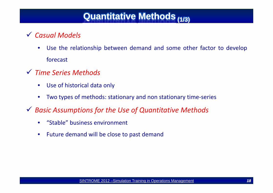
Casual Models
• Use the relationship between demand and some other factor to develop
forecast
Time Series MethodsTime Series Methods
• Use of historical data only
• Two types of methods: stationary and non stationary time series• Two types of methods: stationary and non stationary time‐series
Basic Assumptions for the Use of Quantitative Methods
• “Stable” business environment
• Future demand will be close to past demand
1818SINTROME 2012 –Simulation Training in Operations Management 1818

Quantitative MethodsQuantitative Methods (2/3)(2/3)Quantitative MethodsQuantitative Methods (2/3)(2/3)
Simple Steps to Build Models
• Collect data
• Plot data over time (use of charts in Excel)
• Check for possible cause/effect relationships
• Check for possible patterns (e.g. seasonality, trends etc)
• Reduce/clean data (remove outliers) –if it is applicableReduce/clean data (remove outliers) if it is applicable
• Built forecast model
• Evaluate the model’s accuracy and keep track of model’s accuracy over• Evaluate the model s accuracy and keep track of model s accuracy over
time (redo if needed)
1919SINTROME 2012 –Simulation Training in Operations Management 1919
Quantitative MethodsQuantitative Methods (3/3)(3/3)Quantitative MethodsQuantitative Methods (3/3)(3/3)
2020SINTROME 2012 –Simulation Training in Operations Management 2020
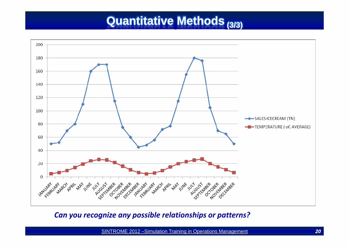
Can you recognize any possible relationships or patterns?

Casual ModelsCasual ModelsCasual ModelsCasual Models
Casual Models
• Relationship between Y (phenomenon that is to be forecasted) and
Xn (n variables that are related to the phenomenon)
• Econometric models are causal models in which the relationship between Y
and (X1 , X2 , . .., Xn ) is linear:
Y = ao + a1 X1 + a2 X2 + … +an XnY ao a1 X1 a2 X2 … an Xn
where a1 , a2 , . . . , an are constants• For examplep
Y= 300 ‐1000 X1 , where:
Y= Sales of apartmentsY Sales of apartments
X1 = Interest rate
If X = 10% (0 1) then Y=200If X1= 10% (0,1) then Y=200
If X1= 5% (0,05) then Y=2502121SINTROME 2012 –Simulation Training in Operations Management 2121

Time Series Methods Time Series Methods (1/5)(1/5)Time Series Methods Time Series Methods (1/5)(1/5)
Time Series Patterns that arise most often:f
• Trend: Long‐term movement in data
• Seasonality: Short‐term regular variations in dataSeasonality: Short term regular variations in data
• Cycles:Wavelike long‐term (more than one year duration) variation in data
• Random Variations Stochasticity: Caused by chance• Random Variations ‐ Stochasticity: Caused by chance
2222SINTROME 2012 –Simulation Training in Operations Management 2222

Time Series Methods Time Series Methods (2/5)(2/5)Time Series Methods Time Series Methods (2/5)(2/5)
Trend:
• Constant increase or decrease of values (linear or nor linear)
eman
d
eman
d
De
DeTime Time
2323SINTROME 2012 –Simulation Training in Operations Management 2323

Time Series Methods Time Series Methods (3/5)(3/5)Time Series Methods Time Series Methods (3/5)(3/5)
Seasonality:
• Repeat of values in fixed time periods (e.g. weeks, months)
• Examples: Fashion, Icecreams, Heating Oil, Gas, Electricity Power etc
ndD
eman
Time
201220112010
2424SINTROME 2012 –Simulation Training in Operations Management 2424
Seasonal variations2010

Time Series Methods Time Series Methods (4/5)(4/5)Time Series Methods Time Series Methods (4/5)(4/5)
Cycles:
• Wavelike variations of more than one year duration
C
2525SINTROME 2012 –Simulation Training in Operations Management 2525
Cycles
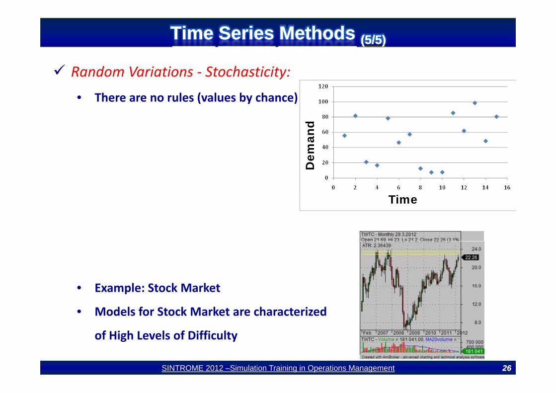
Time Series Methods Time Series Methods (5/5)(5/5)Time Series Methods Time Series Methods (5/5)(5/5)
Random Variations ‐ Stochasticity:
• There are no rules (values by chance)
man
dD
em
TiTime
• Example Stock Market• Example: Stock Market
• Models for Stock Market are characterized
of High Levels of Difficulty
2626SINTROME 2012 –Simulation Training in Operations Management 2626
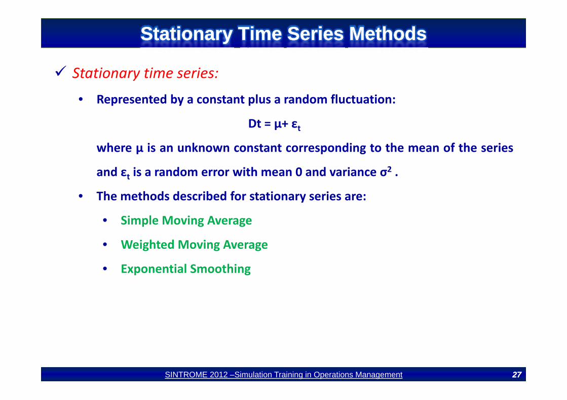
Stationary Time Series MethodsStationary Time Series MethodsStationary Time Series MethodsStationary Time Series Methods
Stationary time series:
• Represented by a constant plus a random fluctuation:
Dt = µ+ εtwhere µ is an unknown constant corresponding to the mean of the series
and εt is a random error with mean 0 and variance σ2 .
• The methods described for stationary series are:The methods described for stationary series are:
• Simple Moving Average
• Weighted Moving Average• Weighted Moving Average
• Exponential Smoothing
2727SINTROME 2012 –Simulation Training in Operations Management 2727

Simple Moving Average Simple Moving Average (1/10)(1/10)Simple Moving Average Simple Moving Average (1/10)(1/10)
Simple Moving Average Forecasting Model (no trend, no
seasonality)y)
• Simple moving average forecasting method uses historical data to
generate a forecast Works well when demand is fairly stable over timegenerate a forecast. Works well when demand is fairly stable over time.
DDDD
t
i
−
+++∑1
NDDD
NF NtttNti
t−−−−= +++
==∑ ...21
NNwhere
Ft= Forecast for period tt p
N= Number of periods used to calculate moving average, and
Di= Actual demand in period i
2828SINTROME 2012 –Simulation Training in Operations Management 2828
Di Actual demand in period i

Simple Moving Average Simple Moving Average (2/10)(2/10)Simple Moving Average Simple Moving Average (2/10)(2/10)
Example 1:
• In the following Table the demand of product A is given per month
Forecasts for N=3 & N=6 periods should be calculated (use of Moving Average)00 2
250 3 175 3 186 5 225 6 285 7 305 8 190
2929SINTROME 2012 –Simulation Training in Operations Management 2929

Simple Moving Average Simple Moving Average (3/9)(3/9)Simple Moving Average Simple Moving Average (3/9)(3/9)
Example 1:
• Formulas for the calculation of Moving Average and Forecast Error (N=3)
3030SINTROME 2012 –Simulation Training in Operations Management 3030

Simple Moving Average Simple Moving Average (4/9)(4/9)Simple Moving Average Simple Moving Average (4/9)(4/9)
Example 1:
• N=3
3131SINTROME 2012 –Simulation Training in Operations Management 3131
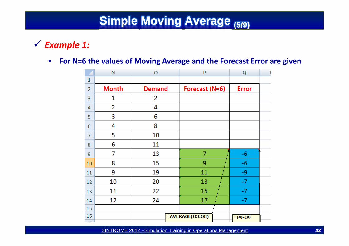
Simple Moving Average Simple Moving Average (5/9)(5/9)Simple Moving Average Simple Moving Average (5/9)(5/9)
Example 1:
• For N=6 the values of Moving Average and the Forecast Error are given
3232SINTROME 2012 –Simulation Training in Operations Management 3232

Simple Moving Average Simple Moving Average ((66//99))Simple Moving Average Simple Moving Average ((66//99))
Example 1:
• N=6
3333SINTROME 2012 –Simulation Training in Operations Management 3333

Simple Moving Average Simple Moving Average ((77//99))Simple Moving Average Simple Moving Average ((77//99))
Example 1:
• For N=3 & N=6 the Moving Average and the Forecast Error are given
3434SINTROME 2012 –Simulation Training in Operations Management 3434

Simple Moving Average Simple Moving Average ((88//99))Simple Moving Average Simple Moving Average ((88//99))
Example 1:
• Moving Average Forecasts lag behind a trend
3535SINTROME 2012 –Simulation Training in Operations Management 3535
• Number of Periods Lag

Simple Moving Average Simple Moving Average ((99//99))Simple Moving Average Simple Moving Average ((99//99))
Advantages:
• Easily understood
• Easily computed
• Provides stable forecasts
Disadvantages:Disadvantages:
• Requires saving lots of past data points: at least the N periods used in the
i imoving average computation
• Lags behind a trend
• Ignores complex relationships in data
3636SINTROME 2012 –Simulation Training in Operations Management 3636

Weighted Moving Average Weighted Moving Average (1/(1/44))Weighted Moving Average Weighted Moving Average (1/(1/44))
Weighted Moving Average Forecasting Model (no trend, no
seasonality)y)
• Based on an n‐period weighted moving average. More recent values in a
series are given more weight in computing the forecast1tseries are given more weight in computing the forecast.1
1 1 2 2 ...
t
i ii t N t t t t t N t N
w Dw D w D w DF
−
= − − − − − − −+ + += =∑
tFN N
= =
where
Ft= Forecast for period tt p
N= Number of periods used to calculate moving average, and
wi = Weight assigned to period i (with Σwi=1)
3737SINTROME 2012 –Simulation Training in Operations Management 3737
wi Weight assigned to period i (with Σwi 1)
Di= Actual demand in period i

Weighted Moving Average Weighted Moving Average (2/(2/44))Weighted Moving Average Weighted Moving Average (2/(2/44))
Example 2:
• In the following Table the demand of product A is given per month
Forecasts for N=3 periods should be calculated (use of Weighted Moving Average)00 2
250 3 175 3 186 5 225 6 285 7 305 8 190
3838SINTROME 2012 –Simulation Training in Operations Management 3838

Example 2:Weighted Moving Average Weighted Moving Average ((33//44))Weighted Moving Average Weighted Moving Average ((33//44))
• For N=3 the values of Weighted Moving Average and the Forecast Errorare given
3939SINTROME 2012 –Simulation Training in Operations Management 3939

Weighted Moving Average Weighted Moving Average ((44//44))Weighted Moving Average Weighted Moving Average ((44//44))
Example 2:
4040SINTROME 2012 –Simulation Training in Operations Management 4040

Exponential SmoothingExponential Smoothing(1/(1/99))Exponential SmoothingExponential Smoothing(1/(1/99))
Exponential Smoothing Model
• A weighted moving average in which the forecast for the next period’s
demand is the current period’s forecast adjusted by a fraction of the
difference between the current period’s actual demand and its forecast.
• More recent data have highest weighting factor a (known as smoothing
constant)constant)
4141SINTROME 2012 –Simulation Training in Operations Management 4141

Exponential SmoothingExponential Smoothing(2/(2/99))Exponential SmoothingExponential Smoothing(2/(2/99))
Exponential Smoothing Model (no trend, no seasonality)
Current forecast is a weighted average of the last forecast and the current
value of demand
New forecast = α * (current observation of demand) + (1‐ α ) * (last forecast)
(1 )F a F a A or+1 1
1 1 1
(1 )( )
t t t
t t t t
F a F a A orF F a A F
− −
− − −
= − +
= + −where
Ft= Forecast for period t
Ft‐1= Forecast for period t‐1
At‐1= Actual demand for period t‐1
4242SINTROME 2012 –Simulation Training in Operations Management 4242
α= a smoothing constant (with 0≤α≥1)
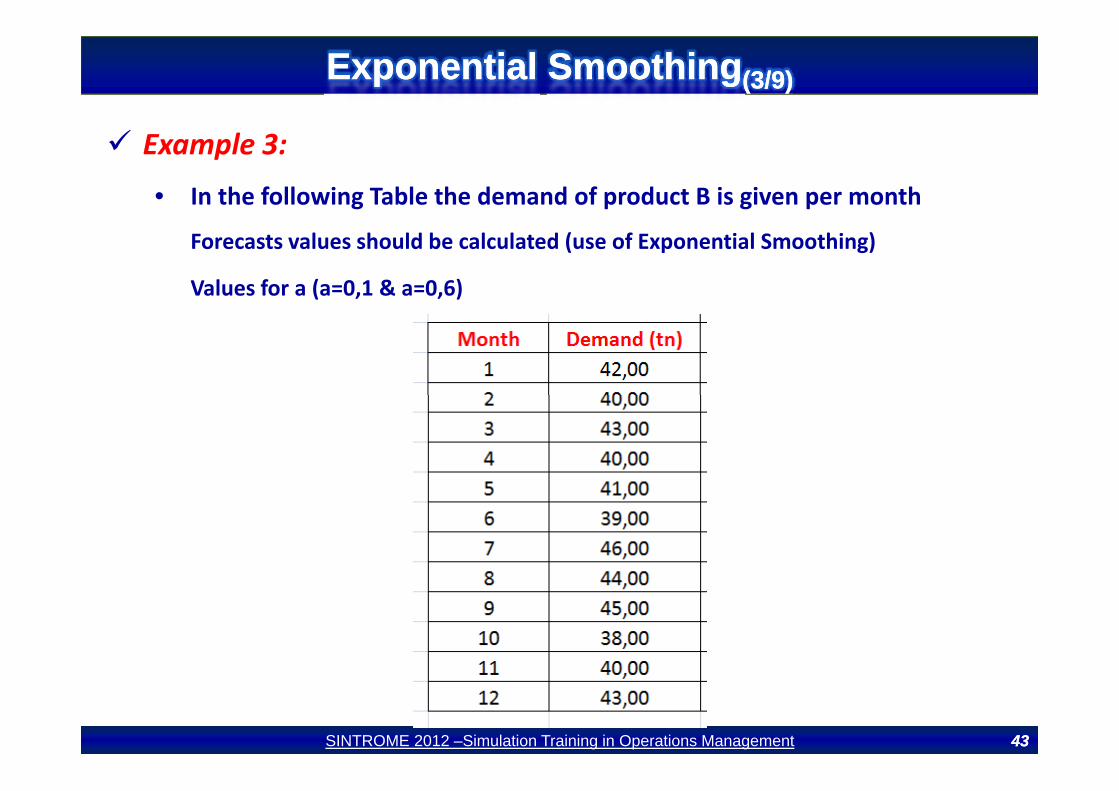
Exponential SmoothingExponential Smoothing(3/(3/99))Exponential SmoothingExponential Smoothing(3/(3/99))
Example 3:
• In the following Table the demand of product B is given per month
Forecasts values should be calculated (use of Exponential Smoothing)
Values for a (a=0,1 & a=0,6) 2 250 3 175 3 186 5 225 6 285 7 305 8 190
4343SINTROME 2012 –Simulation Training in Operations Management 4343

Exponential SmoothingExponential Smoothing((44//99))Exponential SmoothingExponential Smoothing((44//99))
Example 3:
• Values for Forecast and Forecast Error (a=0,1)
4444SINTROME 2012 –Simulation Training in Operations Management 4444

Exponential SmoothingExponential Smoothing((55//99))Exponential SmoothingExponential Smoothing((55//99))
Example 3:
• Graph (a=0,1)
4545SINTROME 2012 –Simulation Training in Operations Management 4545

Exponential SmoothingExponential Smoothing((66//99))Exponential SmoothingExponential Smoothing((66//99))
Example 3:
• Values for Forecast and Forecast Error (a=0,6)
4646SINTROME 2012 –Simulation Training in Operations Management 4646

Exponential SmoothingExponential Smoothing((77//99))Exponential SmoothingExponential Smoothing((77//99))
Example 3:
• Graph (a=0,6)
4747SINTROME 2012 –Simulation Training in Operations Management 4747

Exponential SmoothingExponential Smoothing((88//99))Exponential SmoothingExponential Smoothing((88//99))
Example 3:
• Graph (a=0,3 & a=0,6)
4848SINTROME 2012 –Simulation Training in Operations Management 4848
Observations for Trend?
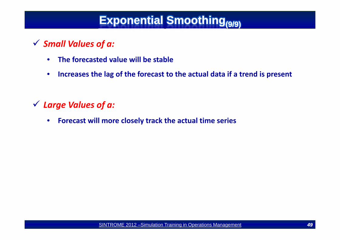
Exponential SmoothingExponential Smoothing((99//99))Exponential SmoothingExponential Smoothing((99//99))
Small Values of a:
• The forecasted value will be stable 2
• Increases the lag of the forecast to the actual data if a trend is present
Large Values of a:
• Forecast will more closely track the actual time series• Forecast will more closely track the actual time series
4949SINTROME 2012 –Simulation Training in Operations Management 4949
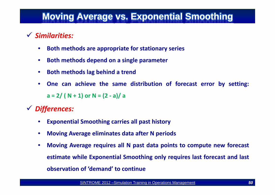
Moving Average vs. Exponential SmoothingMoving Average vs. Exponential SmoothingMoving Average vs. Exponential SmoothingMoving Average vs. Exponential Smoothing
Similarities:
• Both methods are appropriate for stationary series
• Both methods depend on a single parameter
• Both methods lag behind a trend
• One can achieve the same distribution of forecast error by setting:
a = 2/ ( N + 1) or N = (2 ‐ a)/ aa 2/ ( N 1) or N (2 a)/ a
Differences:
E i l S hi i ll hi• Exponential Smoothing carries all past history
• Moving Average eliminates data after N periods
• Moving Average requires all N past data points to compute new forecast
estimate while Exponential Smoothing only requires last forecast and last
observation of ‘demand’ to continue
5050SINTROME 2012 –Simulation Training in Operations Management 5050
Non Stationary Time Series Methods with TrendNon Stationary Time Series Methods with TrendNon Stationary Time Series Methods with TrendNon Stationary Time Series Methods with Trend
Non‐Stationary time series (with Trend):y ( )
• Linear Trend Forecasting Model
• Simple Regression AnalysisSimple Regression Analysis
• Double Exponential Smoothing (Holt’s Method)
5151SINTROME 2012 –Simulation Training in Operations Management 5151

Linear Trend Forecasting Model Linear Trend Forecasting Model (1/4)(1/4)Linear Trend Forecasting Model Linear Trend Forecasting Model (1/4)(1/4)
Linear Trend Forecasting Model (with trend, no seasonality)
The forecasting equation for the linear trend model is:
F btF a b t= +
where
f i dFt = Forecast for period t
t = Specified number of time periods
a = Intercept of the line
b = Slope of the line
5252SINTROME 2012 –Simulation Training in Operations Management 5252

Linear Trend Forecasting Model Linear Trend Forecasting Model (2/4)(2/4)Linear Trend Forecasting Model Linear Trend Forecasting Model (2/4)(2/4)
Calculating a and b
( )n t y t yb
−∑ ∑ ∑2 2
( )( )
y yb
n t t=
−∑ ∑ ∑∑ ∑
y b ta
n−
= ∑ ∑n
where
n = Total number of periods t
t = Period
y = Actual demand in period t
5353SINTROME 2012 –Simulation Training in Operations Management 5353

Linear Trend Forecasting Model Linear Trend Forecasting Model (3/4)(3/4)Linear Trend Forecasting Model Linear Trend Forecasting Model (3/4)(3/4)
Example 4:
• In the following Table the Sales of product X is given per month
The forecasting equation for the linear trend model is requested
5454SINTROME 2012 –Simulation Training in Operations Management 5454

Example 4:Linear Trend Forecasting Model Linear Trend Forecasting Model (4/4)(4/4)Linear Trend Forecasting Model Linear Trend Forecasting Model (4/4)(4/4)
• Values for a, b
5555SINTROME 2012 –Simulation Training in Operations Management 5555
Forecasting Equation: Ft = 143,5+6,3*t
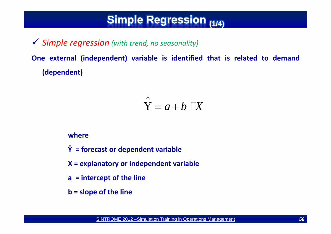
Simple Regression Simple Regression (1/4)(1/4)Simple Regression Simple Regression (1/4)(1/4)
Simple regression (with trend, no seasonality)
One external (independent) variable is identified that is related to demand
(dependent)
a b X∧
Υ = +
where
Ŷ = forecast or dependent variable
X = explanatory or independent variable
a = intercept of the line
b = slope of the line
5656SINTROME 2012 –Simulation Training in Operations Management 5656

Simple Regression Simple Regression (2/4)(2/4)Simple Regression Simple Regression (2/4)(2/4)
Calculating a and b
where
1 n
iD D−
= ∑1
iin =∑
n=number of periods
5757SINTROME 2012 –Simulation Training in Operations Management 5757
Di= actual demand of period i (i=1,….,n)

Simple Regression Simple Regression (3/4)(3/4)Simple Regression Simple Regression (3/4)(3/4)
Example 5:In the following Table the Sales of product X is given per month
The forecasting equation for the simple regression model is requested
Calculation of parameters a & b will be done with a basis of 5 months (set n=5)
5858SINTROME 2012 –Simulation Training in Operations Management 5858

Example 5:Simple Regression Simple Regression (4/4)(4/4)Simple Regression Simple Regression (4/4)(4/4)
• Values for a, b
∧
5959SINTROME 2012 –Simulation Training in Operations Management 5959
Forecasting Equation: 211,4 1,4 X∧
Υ = −

Double Exponential Smooting Double Exponential Smooting (1/4)(1/4)Double Exponential Smooting Double Exponential Smooting (1/4)(1/4)
Double Exponential Smoothing (with trend, no seasonality)
Holt’s method is the most common example, can also be used to forecast
when there is a linear trend present in the data. The method requires
separate smoothing constants for slope and intercept.
The advantage is that once we begin building a forecast model, we canThe advantage is that once we begin building a forecast model, we can
quickly revise the slope and signal constituents with the separate
smoothing coefficientssmoothing coefficients.
6060SINTROME 2012 –Simulation Training in Operations Management 6060

Double Exponential Smooting Double Exponential Smooting (2/4)(2/4)Double Exponential Smooting Double Exponential Smooting (2/4)(2/4)
Double Exponential Smoothing
GSF τ+=where
tttt GSF ττ +=+,
))(1( 11 −− +−+= tttt GSDS αα Intercept at time t
)1()( += GSSG ββ Slope at time t11 )1()( −− −+−= tttt GSSG ββ Slope at time t
Ft,t+τ= Forecast for time τ into the futureDt= Actual Demand in period t t
α = smoothing constant (0 ≤ α ≤ 1)β = smoothing constant for trend (0 ≤ β ≤ 1)
6161SINTROME 2012 –Simulation Training in Operations Management 6161
β g ( β )

Double Exponential Smooting Double Exponential Smooting (3/4)(3/4)Double Exponential Smooting Double Exponential Smooting (3/4)(3/4)
Example 6:In the following Table the Sales of product X is given per month
The forecasting values are requested
Known parameters: a=0,1 & b=0,1
6262SINTROME 2012 –Simulation Training in Operations Management 6262

Double Exponential Smooting Double Exponential Smooting (4/4)(4/4)Double Exponential Smooting Double Exponential Smooting (4/4)(4/4)
Example 6:
6363SINTROME 2012 –Simulation Training in Operations Management 6363
Non Stationary Time Series Methods with SeasonalityNon Stationary Time Series Methods with SeasonalityNon Stationary Time Series Methods with SeasonalityNon Stationary Time Series Methods with Seasonality
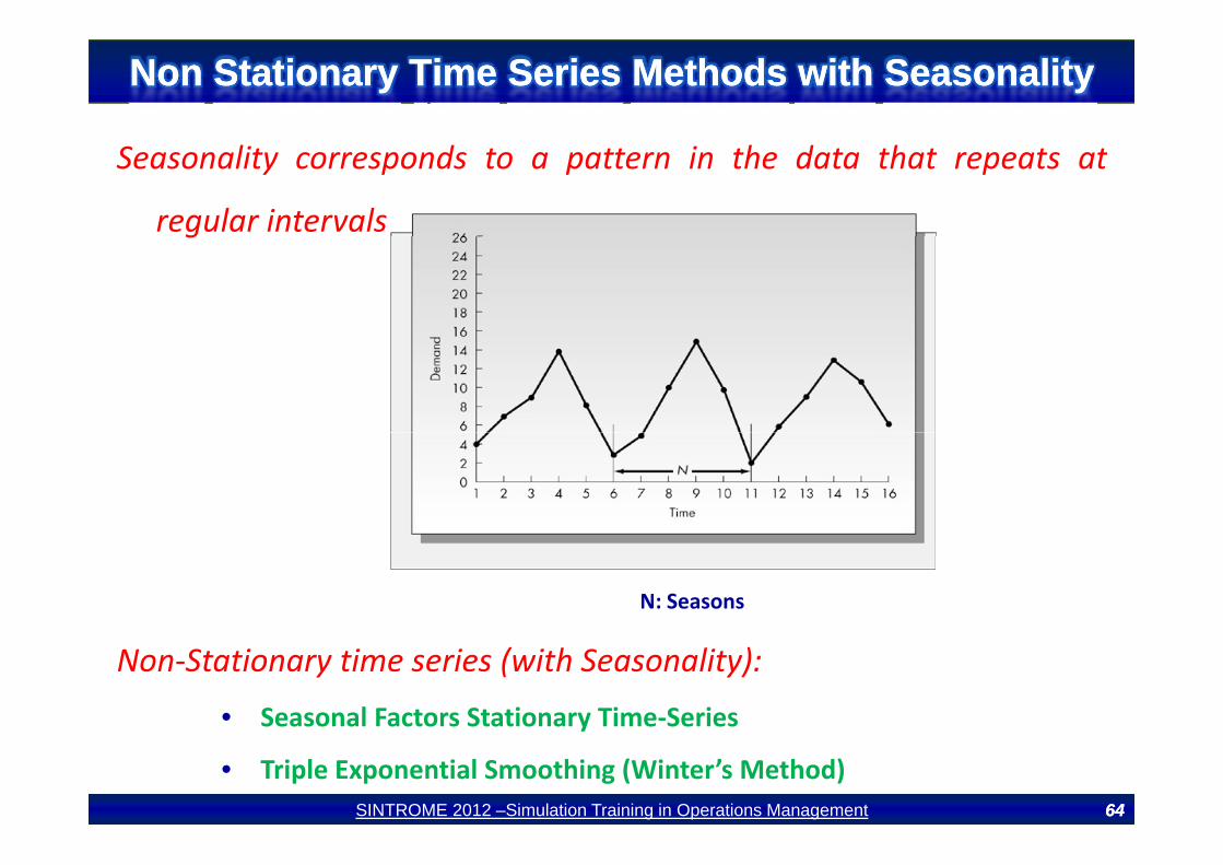
Seasonality corresponds to a pattern in the data that repeats at
regular intervalsg
N: Seasons
Non‐Stationary time series (with Seasonality):
• Seasonal Factors Stationary Time‐Seriesy
• Triple Exponential Smoothing (Winter’s Method)6464SINTROME 2012 –Simulation Training in Operations Management 6464

Seasonal Factors Stationary TimeSeasonal Factors Stationary Time--Series Series (1/3)(1/3)Seasonal Factors Stationary TimeSeasonal Factors Stationary Time--Series Series (1/3)(1/3)
Seasonal Factors Stationary Time‐Series (with seasonality, no trend)
Methodology employedgy p y
• Compute the sample mean of the entire data set (should be at least several
cycles of data)cycles of data)
• Divide each observation by the sample mean (This gives a factor for each
observation)observation)
• Average the factors for the same seasons
Th l i b ill l dd N d d h N• The resulting n numbers will exactly add to N and correspond to the N
seasonal factors.
6565SINTROME 2012 –Simulation Training in Operations Management 6565
Seasonal Factors Stationary TimeSeasonal Factors Stationary Time--Series Series (2/3)(2/3)Seasonal Factors Stationary TimeSeasonal Factors Stationary Time--Series Series (2/3)(2/3)
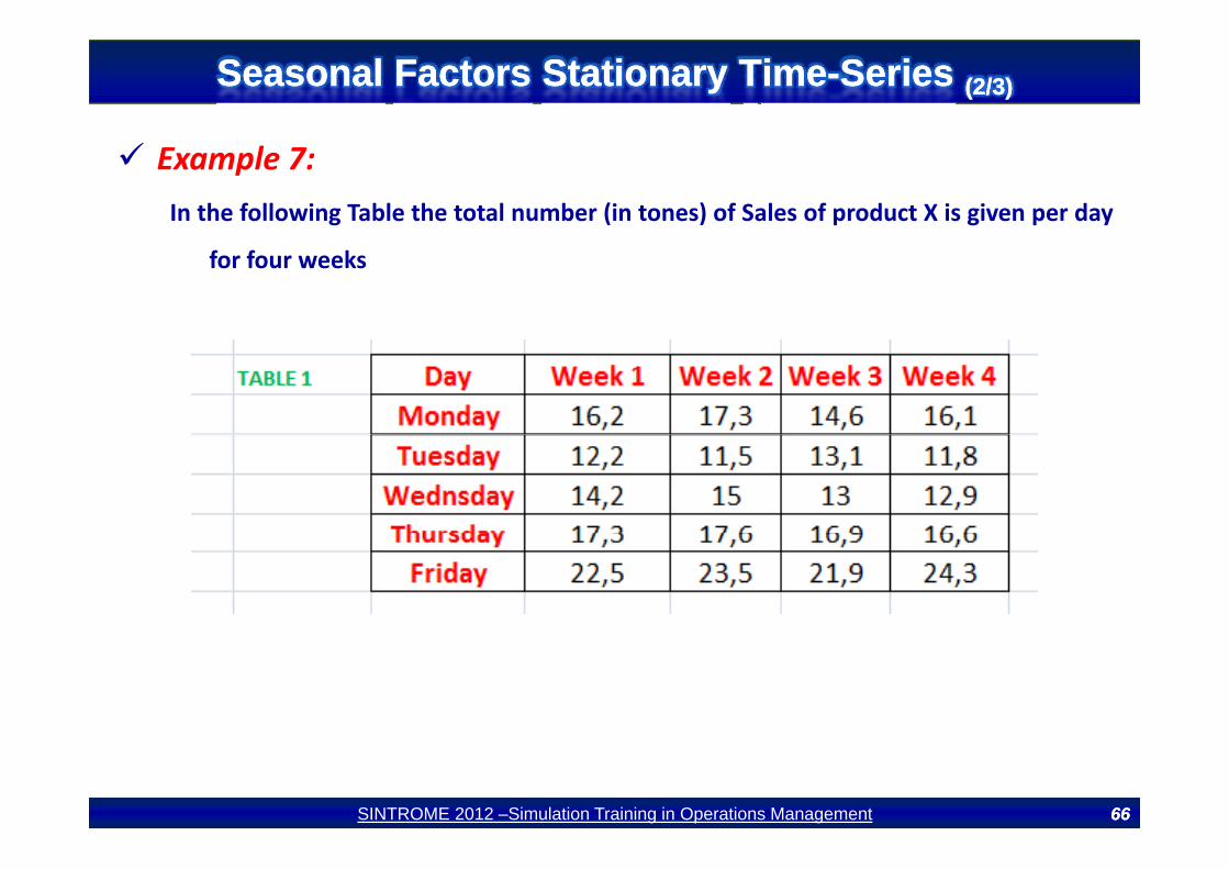
Example 7:In the following Table the total number (in tones) of Sales of product X is given per day
for four weeks
6666SINTROME 2012 –Simulation Training in Operations Management 6666

Seasonal Factors Stationary TimeSeasonal Factors Stationary Time--Series Series (3/3)(3/3)Seasonal Factors Stationary TimeSeasonal Factors Stationary Time--Series Series (3/3)(3/3)
Example 7:
6767SINTROME 2012 –Simulation Training in Operations Management 6767

Triple Exponential Smoothing (Winter’s Method)Triple Exponential Smoothing (Winter’s Method) (1/(1/88))Triple Exponential Smoothing (Winter’s Method)Triple Exponential Smoothing (Winter’s Method) (1/(1/88))
Winter’s Method (with seasonality, with trend)
( )*t t t t t t t NF S tG c= +where
, ( )t t t t t t t NF S tG c+ + −+
( / ) (1 )( )S D c S Gα α= + − + Deseasonalized Time Series Signal1 1( / ) (1 )( )t t t N t tS D c S Gα α− − −= + − +
11 )1()( −+−= GSSG ββ
Deseasonalized Time Series:Signal
Trend11 )1()( −− + tttt GSSG ββ
( ) (1 )tt t N
t
Dc cSγ γ −= + − Seasonal Factors
tSFt,t+t= Forecast for time t into the futureDt= Actual Demand in period tDt Actual Demand in period t α = smoothing constant (0 ≤ α ≤ 1)β = smoothing constant for trend (0 ≤ β ≤ 1)
6868SINTROME 2012 –Simulation Training in Operations Management 6868
β smoothing constant for trend (0 ≤ β ≤ 1)γ = smoothing constant (0 ≤ γ ≤ 1)

Triple Exponential Smoothing (Winter’s Method)Triple Exponential Smoothing (Winter’s Method) ((22//88))Triple Exponential Smoothing (Winter’s Method)Triple Exponential Smoothing (Winter’s Method) ((22//88))
St ti th Wi t ’ M th dStarting the Winter’s Method
•Derive initial estimates of the 3 values: S G and c•Derive initial estimates of the 3 values: St, Gt and ct
•Typically we set: α= 2β = 2γ (A typical value for α=0,2yp y β γ ( yp ,
•Deriving initial estimates takes at least two complete
cycles of data
6969SINTROME 2012 –Simulation Training in Operations Management 6969
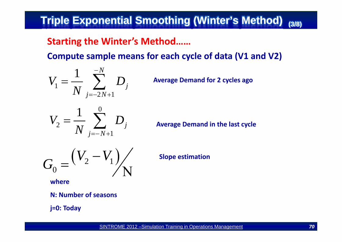
Triple Exponential Smoothing (Winter’s Method)Triple Exponential Smoothing (Winter’s Method) (3/(3/88))Triple Exponential Smoothing (Winter’s Method)Triple Exponential Smoothing (Winter’s Method) (3/(3/88))
St ti th Wi t ’ M th dStarting the Winter’s Method……Compute sample means for each cycle of data (V1 and V2)
12 1
1 N
jj N
V DN
−
+
= ∑ Average Demand for 2 cycles ago
2 1j NN =− +
01V D= ∑21
jj N
V DN =− +
= ∑ Average Demand in the last cycle
( )( )2 10
V VG −= ΝSlope estimation
where
N: Number of seasons
Ν
7070SINTROME 2012 –Simulation Training in Operations Management 7070
j=0: Today

Triple Exponential Smoothing (Winter’s Method)Triple Exponential Smoothing (Winter’s Method) (4/(4/88))Triple Exponential Smoothing (Winter’s Method)Triple Exponential Smoothing (Winter’s Method) (4/(4/88))
E ti ti f Si l d S l F tEstimation of Signal and Seasonal Factor
( )1Ν⎡ ⎤( )0 2 0
12S V G Ν −⎡ ⎤= + ⎢ ⎥⎣ ⎦
Signal Estimation
1t
tDc
N=
⎡ ⎤⎛ ⎞⎛ ⎞0
12
t
iNV j G
⎡ ⎤⎛ + ⎞⎛ ⎞− − ∗⎜ ⎟⎢ ⎥⎜ ⎟⎝ ⎠⎝ ⎠⎣ ⎦Seasonal Factor Estimation
2 1 0for N t− + ≤ ≤
7171SINTROME 2012 –Simulation Training in Operations Management 7171

Triple Exponential Smoothing (Winter’s Method)Triple Exponential Smoothing (Winter’s Method) (5/(5/88))Triple Exponential Smoothing (Winter’s Method)Triple Exponential Smoothing (Winter’s Method) (5/(5/88))
N li i S l F tNormalizing Seasonal Factor
c⎡ ⎤⎢ ⎥
1j
j
i
ccc
−Ν+
⎢ ⎥= ∗Ν⎢ ⎥⎢ ⎥⎢ ⎥⎣ ⎦
∑0
1 0
ii
for N j=⎢ ⎥⎣ ⎦
− + ≤ ≤
∑1 0for N j+ ≤ ≤
7272SINTROME 2012 –Simulation Training in Operations Management 7272

Triple Exponential Smoothing (Winter’s Method)Triple Exponential Smoothing (Winter’s Method) ((66//88))Triple Exponential Smoothing (Winter’s Method)Triple Exponential Smoothing (Winter’s Method) ((66//88))
Example 8:• In the following Table the Sales of product X is given per quarter
7373SINTROME 2012 –Simulation Training in Operations Management 7373

Triple Exponential Smoothing (Winter’s Method)Triple Exponential Smoothing (Winter’s Method) ((7878))Triple Exponential Smoothing (Winter’s Method)Triple Exponential Smoothing (Winter’s Method) ((7878))
Example 8:p
7474SINTROME 2012 –Simulation Training in Operations Management 7474

Triple Exponential Smoothing (Winter’s Method)Triple Exponential Smoothing (Winter’s Method) ((88//88))Triple Exponential Smoothing (Winter’s Method)Triple Exponential Smoothing (Winter’s Method) ((88//88))
Example 8:pTake into account that in quarter 9 (t=1) the observed value of demand is D1=16 and a=0.2,
β=0.1 & γ=0.1β γ
7575SINTROME 2012 –Simulation Training in Operations Management 7575

Synopsis of Forecasting MethodsSynopsis of Forecasting Methods (1/2)(1/2)Synopsis of Forecasting MethodsSynopsis of Forecasting Methods (1/2)(1/2)
7676SINTROME 2012 –Simulation Training in Operations Management 7676

Synopsis of Forecasting MethodsSynopsis of Forecasting Methods (2/2)(2/2)Synopsis of Forecasting MethodsSynopsis of Forecasting Methods (2/2)(2/2)
ChoosingChoosing aa ForecastingForecasting TechniqueTechnique,
No single technique works in every situation
Important factorsp f
•Cost
•Accuracy
Other factors include the availability of:
•Historical data
•Software available•Software available
•Time needed to gather and analyze the data
•Forecast horizon7777SINTROME 2012 –Simulation Training in Operations Management 7777

Evaluating Forecasts Evaluating Forecasts (1/5)(1/5)Evaluating Forecasts Evaluating Forecasts (1/5)(1/5)
ForecastForecast ErrorError inin PeriodPeriod tt:: ,
where
Et = forecast error for Period t
Yt = actual demand for Period t
F forecast for Period tFt = forecast for Period t
7878SINTROME 2012 –Simulation Training in Operations Management 7878

Evaluating Forecasts Evaluating Forecasts (2/5)(2/5)Evaluating Forecasts Evaluating Forecasts (2/5)(2/5)
Criteria for evaluation
Mean Absolute Error (Deviation) (MAD): a MAD of 0 indicates the forecast exactly
predicted demand
Mean Squared Error (Deviation) (MSE): Analogous to variance, large forecast
errors are heavily penalized
Mean Absolute Percentage Error: provides perspective of the true magnitude ofMean Absolute Percentage Error: provides perspective of the true magnitude of
the forecast error
7979SINTROME 2012 –Simulation Training in Operations Management 7979

Evaluating Forecasts Evaluating Forecasts (3/5)(3/5)Evaluating Forecasts Evaluating Forecasts (3/5)(3/5)
Example 9
8080SINTROME 2012 –Simulation Training in Operations Management 8080

Evaluating Forecasts Evaluating Forecasts (4/5)(4/5)Evaluating Forecasts Evaluating Forecasts (4/5)(4/5)
ForecastForecast ErrorError ControlControl ChartChart::
A visual tool for monitoring forecast errors
Used to detect non‐randomness in errors
Forecasting errors are in control if
•All errors are within the control limits
•No patterns such as trends or cycles are presentNo patterns, such as trends or cycles, are present
8181SINTROME 2012 –Simulation Training in Operations Management 8181

Evaluating Forecasts Evaluating Forecasts (5/5)(5/5)Evaluating Forecasts Evaluating Forecasts (5/5)(5/5)
ExampleExample ofof aa ForecastForecast ErrorError ControlControl ChartChart
8282SINTROME 2012 –Simulation Training in Operations Management 8282

Excel
Softwares for ForecastingSoftwares for ForecastingSoftwares for ForecastingSoftwares for ForecastingExcel .
Crystal Ball (CB Predictor).
SAS.
SPSS.SPSS.
MICROFIT.
EVIEWS.
Forecast Pro.
838383838383SINTROME 2012 –Simulation Training in Operations Management 8383

Introduction to CB Predictor™ Introduction to CB Predictor™ (1/16)(1/16)Introduction to CB Predictor™ Introduction to CB Predictor™ (1/16)(1/16)
CBCB Predictor™Predictor™
is an addition to the Crystal Ball suite of decision intelligence
products
i f th l d f t i i tiis for the planner and forecaster in every organization
has a wide range of forecasting applicationshas a wide range of forecasting applications
runs on several versions of Microsoft Windows and Microsoft
Excel
Oracle® CB Predictor User Manual Release 11.1.1.1.00
8484SINTROME 2012 –Simulation Training in Operations Management 8484

Introduction to CB Predictor™ Introduction to CB Predictor™ (2/16)(2/16)Introduction to CB Predictor™ Introduction to CB Predictor™ (2/16)(2/16)
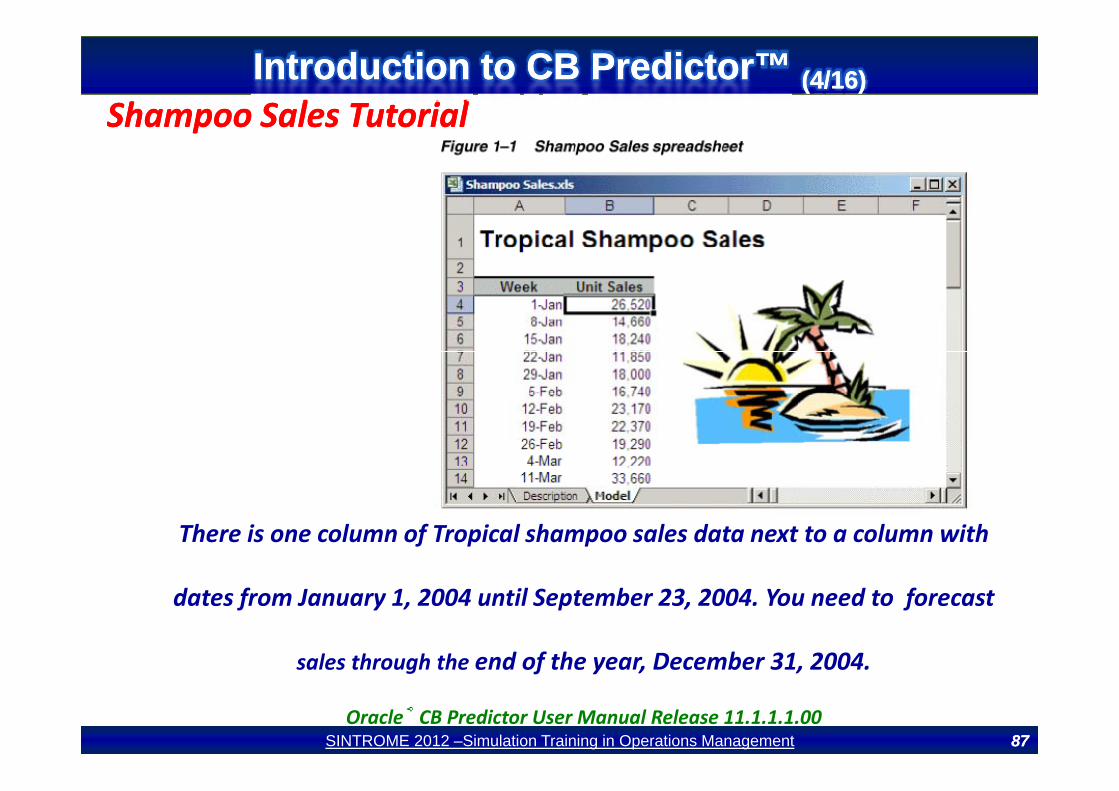
ShampooShampoo SalesSales TutorialTutorial
Role: Sales manager for Tropical Cosmetics Co.
Product: Tropical Shampoo (company’s latest product)
Hi t i l D t S l f 9 th i dHistorical Data: Sales for a 9 month period
Decision: Forecast the rest of the year’s sales of shampoo andDecision: Forecast the rest of the year s sales of shampoo and
decide whether to recommend investing in advertising or
enhancements for this product.
Oracle® CB Predictor User Manual Release 11.1.1.1.00
8585SINTROME 2012 –Simulation Training in Operations Management 8585

Introduction to CB Predictor™ Introduction to CB Predictor™ (3/16)(3/16)Introduction to CB Predictor™ Introduction to CB Predictor™ (3/16)(3/16)
ShampooShampoo SalesSales TutorialTutorial
1: Start Crystal Ball and Excel.
2: Open the Shampoo Sales spreadsheet from the Examples
folder.
By default, the file is stored in this folder:
C:\Program Files\Oracle\Crystal Ball\Examples\CB Predictor Examples.
Oracle® CB Predictor User Manual Release 11.1.1.1.008686SINTROME 2012 –Simulation Training in Operations Management 8686
ShampooShampoo SalesSales TutorialTutorialIntroduction to CB Predictor™ Introduction to CB Predictor™ (4/16)(4/16)Introduction to CB Predictor™ Introduction to CB Predictor™ (4/16)(4/16)
ShampooShampoo SalesSales TutorialTutorial
There is one column of Tropical shampoo sales data next to a column with
dates from January 1, 2004 until September 23, 2004. You need to forecast
sales through the end of the year December 31 2004sales through the end of the year, December 31, 2004.
Oracle® CB Predictor User Manual Release 11.1.1.1.008787SINTROME 2012 –Simulation Training in Operations Management 8787

ShSh S lS l T t i lT t i l
Introduction to CB Predictor™ Introduction to CB Predictor™ (5/16)(5/16)Introduction to CB Predictor™ Introduction to CB Predictor™ (5/16)(5/16)
ShampooShampoo SalesSales TutorialTutorial
3: Select cell B4. Selecting any one cell in your data range,
headers, or date range initiates CB Predictor’s "Intelligent Input"
t l t ll th fill d dj t llto select all the filled, adjacent cells.
4: Select Run > CB Predictor. This command is only available if
i l i i i d h l Ifno simulation is running and the last run was reset. If necessary,
wait for a simulation to stop or reset the last simulation.
Oracle® CB Predictor User Manual Release 11.1.1.1.00Oracle CB Predictor User Manual Release 11.1.1.1.00
8888SINTROME 2012 –Simulation Training in Operations Management 8888
ShSh S lS l T t i lT t i l
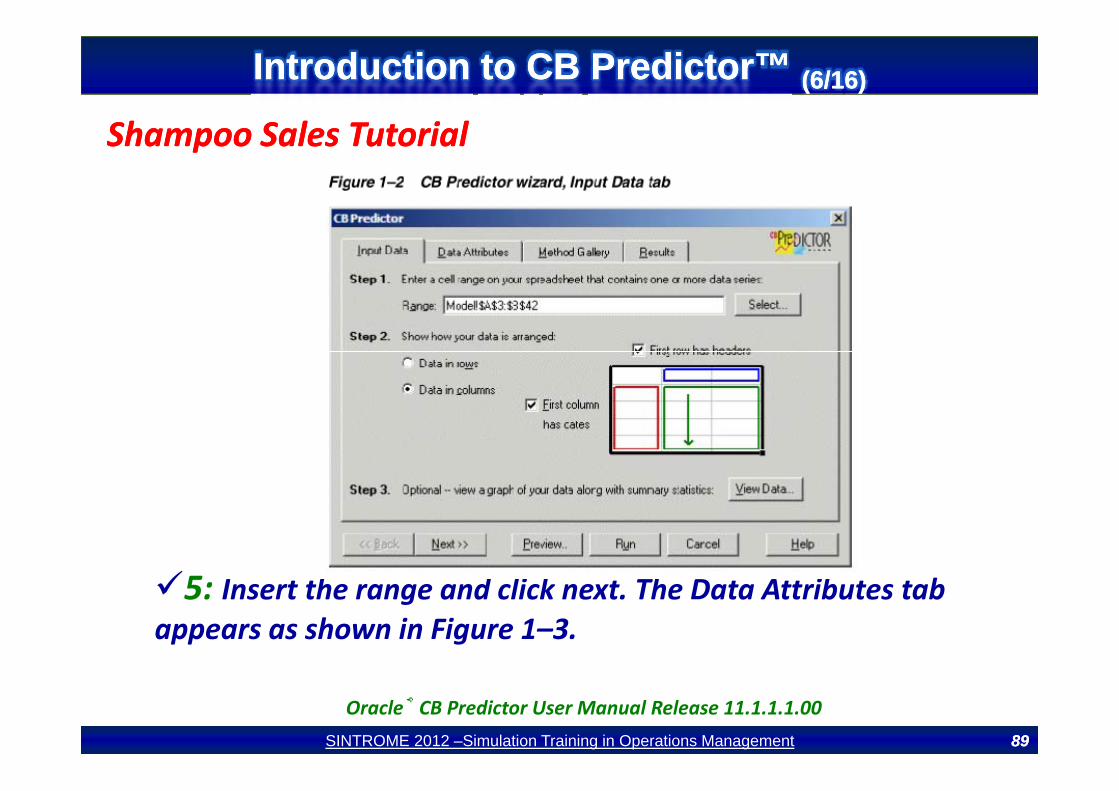
Introduction to CB Predictor™ Introduction to CB Predictor™ (6/16)(6/16)Introduction to CB Predictor™ Introduction to CB Predictor™ (6/16)(6/16)
ShampooShampoo SalesSales TutorialTutorial
5: Insert the range and click next. The Data Attributes tab appears as shown in Figure 1–3.
Oracle® CB Predictor User Manual Release 11.1.1.1.008989SINTROME 2012 –Simulation Training in Operations Management 8989

ShSh S lS l T t i lT t i l
Introduction to CB Predictor™ Introduction to CB Predictor™ (7/16)(7/16)Introduction to CB Predictor™ Introduction to CB Predictor™ (7/16)(7/16)
ShampooShampoo SalesSales TutorialTutorial
Oracle® CB Predictor User Manual Release 11.1.1.1.00
9090SINTROME 2012 –Simulation Training in Operations Management 9090
ShSh S lS l T t i lT t i l
Introduction to CB Predictor™ Introduction to CB Predictor™ (8/16)(8/16)Introduction to CB Predictor™ Introduction to CB Predictor™ (8/16)(8/16)
ShampooShampoo SalesSales TutorialTutorial6:Under Step 4:
A. Select "weeks" from the Data Is In list.
B. Set the data to have no seasonality. (You have less thanB. Set the data to have no seasonality. (You have less thantwo complete seasons (cycles) of data, so cannot useseasonality.
7: Under Step 5, make sure that Use Multiple LinearRegression is not checked. (You did not choose regressiong ( gbecause you have only one series of data, so there are nodependencies between series requiring regression.)
8: Click Next
Oracle® CB Predictor User Manual Release 11.1.1.1.009191SINTROME 2012 –Simulation Training in Operations Management 9191

ShSh S lS l T t i lT t i l
Introduction to CB Predictor™ Introduction to CB Predictor™ (9/16)(9/16)Introduction to CB Predictor™ Introduction to CB Predictor™ (9/16)(9/16)
ShampooShampoo SalesSales TutorialTutorial
Oracle® CB Predictor User Manual Release 11.1.1.1.00
9292SINTROME 2012 –Simulation Training in Operations Management 9292

ShSh S lS l T t i lT t i l
Introduction to CB Predictor™ Introduction to CB Predictor™ (10/16)(10/16)Introduction to CB Predictor™ Introduction to CB Predictor™ (10/16)(10/16)
ShampooShampoo SalesSales TutorialTutorial9: Click Select All. This selects all the time‐series forecasting
methods, but CB Predictor doesn’t use the seasonal methods,since you indicated that your data were not seasonal. CBPredictor forecasts your values using each of the selectedPredictor forecasts your values using each of the selectedmethods and ranks them according to how well they fit thehistorical data. CB Predictor uses the seasonal methods as wellas the nonseasonal methods if you indicate on the DataAttributes tab that your data series have seasonality.
10: Click Next. The Results tab appears as shown in Figure 1–5.The only output selected by default is Paste Forecast, which addsthe forecasted values to the end of your historical data as shownin Figure 1–5.
Oracle® CB Predictor User Manual Release 11.1.1.1.00
9393SINTROME 2012 –Simulation Training in Operations Management 9393

ShSh S lS l T t i lT t i l
Introduction to CB Predictor™ Introduction to CB Predictor™ (11/16)(11/16)Introduction to CB Predictor™ Introduction to CB Predictor™ (11/16)(11/16)
ShampooShampoo SalesSales TutorialTutorial
Oracle® CB Predictor User Manual Release 11.1.1.1.00
9494SINTROME 2012 –Simulation Training in Operations Management 9494
ShSh S lS l T t i lT t i l
Introduction to CB Predictor™ Introduction to CB Predictor™ (12/16)(12/16)Introduction to CB Predictor™ Introduction to CB Predictor™ (12/16)(12/16)
ShampooShampoo SalesSales TutorialTutorial11: Under Step 7, forecast the weekly sales for the rest of the
year by entering 13 in the field.
12: Click Preview. The Preview Forecast dialog appears. Itpresents a graph with historical data, fitted data, forecastvalues, and confidence intervals as shown in Figure 1–6.
O l ® CB P di t U M l R l 11 1 1 1 00Oracle® CB Predictor User Manual Release 11.1.1.1.00
9595SINTROME 2012 –Simulation Training in Operations Management 9595

ShSh S lS l T t i lT t i l
Introduction to CB Predictor™ Introduction to CB Predictor™ (13/16)(13/16)Introduction to CB Predictor™ Introduction to CB Predictor™ (13/16)(13/16)
ShampooShampoo SalesSales TutorialTutorial
Oracle® CB Predictor User Manual Release 11.1.1.1.00
9696SINTROME 2012 –Simulation Training in Operations Management 9696

ShSh S lS l T t i lT t i l
Introduction to CB Predictor™ Introduction to CB Predictor™ (14/16)(14/16)Introduction to CB Predictor™ Introduction to CB Predictor™ (14/16)(14/16)
ShampooShampoo SalesSales TutorialTutorial13: In the Preview Forecast dialog, click the Method field. The
field lists all the methods CB Predictor tried, in order from thebest‐fitting method (designated by the word "Best") to theworst‐fitting method CB Predictor calculates the forecastedworst‐fitting method. CB Predictor calculates the forecastedvalues from the method that best fits the historical data. In thiscase, the method is Double Exponential Smoothing. The, p gforecasted values appear as a blue line extending to the right ofthe historical data (green) and the fitted values (also in blue).b d b l h f d l i h fid i lAbove and below the forecasted values is the confidence interval
(in red), showing the 5th and 95th percentiles of the forecastedvaluesvalues.
Oracle® CB Predictor User Manual Release 11.1.1.1.00
9797SINTROME 2012 –Simulation Training in Operations Management 9797

ShSh S lS l T t i lT t i l
Introduction to CB Predictor™ Introduction to CB Predictor™ (15/16)(15/16)Introduction to CB Predictor™ Introduction to CB Predictor™ (15/16)(15/16)
ShampooShampoo SalesSales TutorialTutorial14: Click Run. The program pastes the forecasted values at the
end of the historical data (in bold), extending the date series aswell. The forecasted values were forecasted using the bestmethod as shown in the Preview dialogmethod, as shown in the Preview dialog.
Oracle® CB Predictor User Manual Release 11.1.1.1.00
9898SINTROME 2012 –Simulation Training in Operations Management 9898

ShSh S lS l T t i lT t i l
Introduction to CB Predictor™ Introduction to CB Predictor™ (16/16)(16/16)Introduction to CB Predictor™ Introduction to CB Predictor™ (16/16)(16/16)
ShampooShampoo SalesSales TutorialTutorial
Decision: Recommendation for further funding on this product
Oracle® CB Predictor User Manual Release 11.1.1.1.00
9999SINTROME 2012 –Simulation Training in Operations Management 9999
