A theory of nonmonotonic rule systems

W. Marek,1 A. Nerode2 and J. Remmel3

1 Introduction

In mathematics, a consequence drawn by a deduction from a set of premises canalso drawn by the same deduction from any larger set of premises. The deductionremains a deduction no matter how the axioms are increased. This is monotonicreasoning, much imitated in other, less certain, disciplines. The very natureof monotonic reasoning makes mathematical proofs permanent, independentof new information. Thus it has been since Euclid and Aristotle. Theoremswith complete proofs are never withdrawn due to later knowledge. It is littleexaggeration to say that mathematicians never reject the completed proofs oftheir predecessors, except to complain about their constructivity.

Mathematicians build directly on the works of their forebearers stretchingback two and a half millenia to Euclid. Our current mathematical reasoning ismerely a fleshed-out version of Euclid’s. Monotonic reasoning marks theoreticalmathematics as a discipline. The traditional systems of mathematical logic aremonotonic since they simple reflect mathematical usage. Tarski [43] described acalculus of deductive systems and captured in a simple way the general conceptof a monotonic formal system. His formulation includes all logics traditionallystudied, intuitionistic, modal, and classical. He did not qualify his definition,as we do, with the adjective “monotone,” because there were no other systemsstudied at that time.

Minsky [32] suggested that there is another sort of reasoning which is notmonotonic. This is reasoning in which we deduce a statement based on theabsence of any evidence against the statement. Such a statement is in thecategory of beliefs rather than in the category of truths. Modern science offers

1Department of Computer Science, University Kentucky, Lexington, KY 40506–0027. Cur-

rently in Mathematical Sciences Institute at Cornell University. Work partially supported by

N.S.F. grant RII 8610671 and Kentucky EPSCoR program and the ARO contract DAAL03-

89-K-01242Mathematical Sciences Institute, Cornell University, Ithaca, NY 14853. Work partially

supported by NSF grant MCS-83-01850 and ARO contract DAAG629-85-C-0018.3Department of Mathematics, University of California at San Diego, La Jolla, CA 92903.

Work partially supported by NSF grant DMS-87-02473.

1

as a tool for establishing provisional beliefs statistics, but in many instances wehave no basis for applying statistics, due to a lack of governing distributions orsamples for the problem at hand.

What role does belief play in our affairs? Often we must make sharp “yesor no” decisions between alternative actions. There may be no deductive orstatistical base which justifies our choice, but we may not be able to wait formissing information, it may never materialize anyway. Often all we have as abasis for decision is surmise; that is, deductions from beliefs as well as truthsand statistically derived statements. These beliefs are often accepted and usedas premises for deduction and choice of action due to an unquantified lack ofevidence against them.

A philosopher’s much-quoted example is about Tweety. We observe onlybirds that can fly, and accept the belief that all birds can fly from the absence ofevidence for the existence of non-flying birds. We are told that Tweety is a bird,and conclude that Tweety can’t fly using our belief as premise. Later, we observethat Tweety is a pet ostrich and clearly can’t fly. We reject our previous beliefset and conclusions as a basis for decision making, and are forced to choose a newbelief set. The new set of beliefs may also include equally uncertain statements,accepted due to a lack of evidence against. But we blithly draw consequencesfrom the new belief set and make decisions on that basis till contrary evidenceon some accepted belief is garnered, at which time we again have to acquire anew set of beliefs.

This has happened in the history of practically every subject except math-ematics. The principles of physics, or biology, have been changed with everyscientific revolution, even though unreflective practitioners of each age thinkthat final principles have been found. Even for mathematics, the Dutch mathe-matician and philosopher L.E.J. Brouwer would have argued that the belief intheorems established by “non-constructive methods” was unjustified, and thata new belief set based on constructive principles should be adopted in its place.Other mainstream mathematicians such as Hilbert did not agree with this po-sition. Some philosophers of mathematics living now would argue that, evenwithin classical mathematics, the independence proofs for propositions of settheory, such as the continuum hypothesis or the axiom of choice, indicate thereare several incompatible axiomatic systems which, as belief sets, could be thefoundation of mathematics.

One can envisage making up non-monotone logics describing the mathemat-ical nature of belief. The exact result depends on the definition chosen for “lackof evidence against”. McCarthy [30], initiated the study of non-monotonicitywith his notion of circumscription. With all relation symbols but one, R, of amodel (the world we are discussing) held fixed, and given axioms ϕ(R) relatingthat R to the other (fixed) relations of the model, the belief should be that,lacking further evidence to the contrary, we should posit that R denotes theleast relation R, if any, satisfying ϕ(R). If further evidence in the form of an

2

axiom ψ(R) becomes available, then we should believe that R denotes the leastR satisfying (ϕ ∧ ψ)(R), if any, instead, in a changed belief set.

There are now many different non-monotonic system, abstracted from differ-ent questions in computer science and AI. Among the other systems that havebeen studied are

The theory of multiple believers of Hintikka, [18].

Truth Maintenance systems of Doyle, [8]

Default logic of Reiter, [40]

Autoepistemic logic of Moore, [34]

Theory of individual and common knowledge and belief of Halpern andMoses [17]

Logic programming with negation as failure [?].

This, by no means, exhausts the list. What issues in artificial intelligence orcomputer science motivates these systems?

Suppose that we build a robot in a “blocks world” to navigate in a roomand avoid obstacles and perform simple tasks, such as crossing the room withvariable obstacles. We want the robot to learn principles from experience as tohow to cross the room. At any given point, one may imagine that the robotshould have a consistent deductively closed set of beliefs which are the currentbasis for its actions, including such provisional beliefs as “I can always traversethe left edge of the room since there has never been anything in the way there”.But when such a principle is contradicted by new obstacles, the robot has tochoose another belief set. So an important problem is to define what a belief setis and how to compute them and how to update them based on new evidence.Moore’s autoepistemic logic [34], is really a first try at this problem, mostly forpropositional logic.

In computers, the operating system and program obey rules which computehow to change state. In the absence of exceptional behaviour, such as errorconditions or failures to access resources, there is a system of decision rules(beliefs) computing how to change the state of the machine in this “normalbehavior”, or “default” case. But when an exceptional behavior happens, weare thrown to a different set of decision rules for change of state, a different setof “beliefs”. One wants to be able to deduce what is true of the machine instates when it is a particular such “belief set”. A logic for dealing with one suchbelief set at a time is Reiter’s default logic.

In databases, facts and rules are stored as entries (the PROLOG model).Often also the database computes and stores conclusions, such as summarystatistics or rules or tables computed from the database. These act as a de-ductive base for the set of current beliefs. When we query the database, we

3

are asking for consequences of this belief set. When we update the database,all old entries that have changed have to be replaced, every consequence thatuses these entries has to be recomputed and changed too. This is the processof replacing an old belief set by a new one. One often makes decisions on thebasis of the absence of information in the database as well. A logic appropriatefor describing a single such belief set is Doyle’s truth-maintenance system [8].See also de Kleer [6]. Also stable models for logic programming with negationas failure ([10]) arise in this way.

We expressed these examples informally in terms of the anthropomorphicnotion of belief so as to bring out their common features. The actual non-monotonic logics have much in common, and a number of translations betweenthem have been proposed ([23], [12],[13], [39],[28]). They have been investi-gated principally for propositional logic. Predicate versions suitable for actualapplications are, up to now, pretty minimal.

Study of monotonic rule systems can be traced to the work of Post on “pro-duction systems” and to work of Tarski on the abstract properties of conse-quence relation for classical logic systems. The investigation of nonmonotoniccomponent is of much more recent nature and seems to appear first in the workof Reiter on default logic. Reiter’s investigations involved finding a naturalextension of classical logic which allows one to handle the negative information.

Independently Clark, and subsequently Apt, Blair and Walker, and also (ex-tending their work) Gelfond and Lifschitz, studied “negation as failure” in logicprogramming. It has turned out that these investigations are in a common direc-tion. The mutual relations were uncovered by Bidoit and Froidevaux and Marekand Truszczynski, who exhibited the precise nature of the connection betweenlogic programming and default logic. The reevaluation of default extensions interms of “context-dependent proofs” by Marek and Truszczynski, which has itsroots in the Apt, Blair and Walker’s “elementary interpreter”, for which it mayserve as a clarifying definition, is a point of departure for the investigations ofthis paper. Here, drawing on all the research mentioned above for inspiration,we present a coherent unified theory of nonmonotonic formal systems.

At our level of abstraction we finally saw that non-monotone systems per-vade ordinary mathematical practice. There is no sign of any realization of theexistence of such mathematical examples in the previous non-monotonic logicliterature. Perhaps these connections can only be seen by having a commonabstract notion. What this commonality does for us is to make available knownmathematical techniques from other areas of conventional mathematics for con-structing and classifying belief sets (extensions), and simultaneously make ev-ident a common thread among disparate parts of mathematics and disparatenon-monotonic systems from artificial intelligence and computer science.

On the level of Mathematical Philosophy there is a connection worth statingas well. Non-monotone reasoning takes place during the process of discovery

4

of mathematical theorems, when one posits temporarily some proposition onthe basis that there is no evidence against it, and explores the consequencesof such a belief until new mathematical facts force their abandonment. Thesenon-monotone belief sets have their traces eradicated when final belief sets areachieved and demonstrative proofs are finished and published. The only hint ofprovisional belief sets left in mathematical papers is in the motivational remarksexplaining what obstacles were overcome and by what changes in viewpoint theproof was achieved.

Here is the main definition. A non-monotone rule system consists of a setU and a set of triples (α, β, γ) called rules, where α = (α1, . . . , αk) is a finitesequence of elements of U , called premises, β = (β1, . . . , β1) is a finite sequenceof elements from U , called guards, and γ is an element of U . This is written,generalizing a notation of default logic, as

α1 . . . , αn:β1, . . . , βkγ

The informal reading is: From α1, . . . , αk being established, and β1, . . . , βk notbeing established now or ever, conclude γ. You may substitute “computed” for“established” for an informal reading in many applications. A subset S of U iscalled deductively closed if for every rule of the system, whenever α1, . . . , αk arein S and β1, . . . , βn are not in S, then γ is in S. There are no variables here,these are not schema, this version is not the one appropriate for non-monotonepredicate logics. Nonmonotonic predicate logics cannot be exposited in a fewlines and we defer that to a later paper.

The intersection of all deductively closed sets containing a set I is generallynot deductively closed. But the intersection of a descending chain of deductivelyclosed sets is deductively closed, and I may be contained in many minimal de-ductively closed sets over I. In the context of nonmonotone logic the intersectionof all deductively closed sets containing I is a (non-deductively closed) set, calledthe the set of secure consequences of I. These are the propositions a “skepti-cal reasoner” would take as beliefs based on I. The most important notion ofcontemporary nonmonotonic logic is that of extension. For a fixed subset S ofU , one defines (finite) derivations from I, where all guards encountered are out-side S, all premises encountered are conclusions of previous rules or in I. Thisdefines the set CS(I) of S-consequences of I. Extensions are those S such thatS = CS(I). These are minimal deductively closed sets containing I, but notconversely. These represent the “deductively closed, grounded, belief sets” thatcontain I. In these sets, if the negative guards are all obeyed, we are reducedto monotone reasoning. See Section 2 for the exact definition.

These simple definitions capture the common content of the several theoriesof non-monotonicity listed above, and of many mathematical theories as well.For example, the set of all marriages of the “marriage problem” can be formu-lated as exactly the set of all extensions in a non-monotone rule system; similarlyfor the set of all k-colorings of graphs, the set of chain covers of a partial order,

5

the Stone space of all maximal ideals of a Boolean algebra, etc. Similarly, fora commutative ring with unit there is a non-monotone rule system such thatthe deductively closed sets are the prime ideals, the McCoy radical (the set ofnilpotents) is the set of secured consequences of {0}, etc. There are similar non-monotonic systems associated with virtually every algebraic systremn for whichradicals of some sort have been defined and characterized. These mathematicalexamples have suggested a whole new set of techniques for finding extensions be-cause of the availability of algorithms already investigated in the mathematicalliterature on one or another of these problems, not previously known to be rele-vant in the artificial intelligence community. They not arise in logic, but reallyin operations research. Finally, in recursion theory, prioric constructions can beconstrued as non-monotone systems, sets constructed by the priority argumentas extensions. These ideas give many constructions of recursively enumerableextensions.

We spend a lot of effort in both this and subsequent papers to answer thefollowing question. Exactly how complicated is the set of extensions of a recur-sively enumerable nonmonotonic system, and what is its structure? This is theanalogue of the classical logic question, how complicated is the set of completetheories containing a recursively enumerable theory, and what is its structure?In classical logic, this leads to analyzing the character of the set of maximal ide-als containing given recursively enumerable ideal in a recursively presented freeBoolean Algebra, a subject in which two of the authors have a lot of experience(see [42], [35]). The simplest case covering many nonmonotonic systems aris-ing from mathematics is that of “highly recursive” nonmonotone rule systems.There, it turns out that extensions can be, up to a one-to-one recursive map,exactly any bounded Π0

1 class os sets of natural numbers. So, even in this case,the computational problems are of the same level of difficulty as (say) solving“marriage problem” for highly recursive societies, or finding of recursively pre-sented formally real field ([31]), or finding an abcissa between 0 and 1 where agiven recursive continuous function on [0,1] takes a maximum value ([19]). Nowthis recursion-theoretic methodology can be refined to give complexity-theoreticresults on the same problems about extensions, as has been done in algebra byNerode and Remmel in [36], [37], and [38]. Since this is a more delicate matterthan recursion theory, these developments are deferred again to a later paper.

Next, we turn to investigations of the semantics for nonmonotonic rule sys-tems. The fundamental common semantics we have found comes from Lω1ω,and generalizes the Clark completion of logic programming. It is perfectly gen-eral, and gives systematic semantics and completeness for all the nonmonotoniclogics discussed above. Such uniform semantics are new. Some of the subjectsnever before had a decent semantics. We find semantical representations ofextensions, weak extensions and deductively closed sets. This representation re-quires creation of an additional infinitary language LS which properly encodesnot only rules as “first order objects”, but also additional (infinitary) objects al-lowing characterization of the intended structures (extensions, weak extensions

6

etc.). The previously established characterization of default logic, in termsof nonmonotonic rule systems, provides us with a semantics for default logic.This semantics, in opposition to the attempt of Etherington, satisfies Tarski’sconditions. That is, it allows us to introduce for defaults (virtual) negations,conjunctions etc, and also a natural entailment relation. Finally, the Lω1,ω proofprocedures also yield new algorithms based on recursive well-founded trees.

This short summary indicates that there is a great wealth of problems andresults which naturally arise from nonmonotonic rule systems. Our study de-lineates the role of (parametized) deducibility in nonmonotonic logics. This, inturn, connects our work naturally with studies of inductive definability. Thelatter indicates that logic programming will profit by less emphasis on predi-cate calculus, and more emphasis on inductive definability. Although this is aparadigm different from Kowalski’s, we do not claim that this is the only “cor-rect” position. But we do claim that it leads to a new direction for research.

The predicate logic case is not treated in this paper. It will come out from aschematic version of our theory, analogous to Post production systems. There, Uis the set of all strings of an alphabet. There are typed “metavariables” rangingover specific subsets of U called “types”, there are “metastrings”. These arebuilt from the alphabet of U and string variables, as sequence of elements ofU and variables. Rules are of the same form as before, but use metastringsinstead of strings. This point of view gives rise not only to a general theory,but also gives outright syntax, semantics, and completeness for new predicateversions of all the logics mentioned above. It also gives non-monotone classical,or intuitionistic, or modal predicate and propositional logics.

2 Nonmonotonic formal systems

Inspired by Reiter [40], and Apt [?], we introduce the notion of a nonmono-tonic formal system < U,N >. A nonmonotonic rule of inference is a triple< P,G,ϕ >, where P = {α1, . . . , αn}, G = {β1, . . . , βm} are finite lists ofobjects from U and ϕ ∈ U . Each such rule is written in form

r =α1, . . . , αn:β1, . . . , βm

ϕ(1)

Here {α1, . . . , αn} are called the premises of rule r, {β1, . . . , βm} are called theguards of rule r.

Either, or both, lists P , G may be empty. If P = G = ∅ then the rule r iscalled an axiom.

A nonmonotonic formal system is a pair < U,N >, where U is a non-emptyset and N is a set of nonmonotonic rules.

A monotonic formal system is a nonmonotonic system in which each rule

7

has no guards. That is, each monotonic formal system can be identified withthe nonmonotonic system in which every monotonic rule is given an empty setof guards.

A subset S ⊆ U is called deductively closed if for every rule of N , if allpremises α1, . . . , αn are in S and all guards β1, . . . , βm are not in S then theconclusion ϕ belongs to S.

In nonmonotonic systems, deductively closed sets are not generally closedunder arbitrary intersections as in monotone case. But deductively closed setsare closed under intersections of descending chains. By the Kuratowski-ZornLemma, any I ⊆ U is contained in at least one minimal deductively closed set.The intersection of all the deductively closed sets containing I is called the setof secured consequences of I. This set is also the intersection of all minimaldeductively closed sets containing I. Deductively closed sets are thought of asrepresenting possible “points of view”. The intersection of all deductively closedsets containing I represents the common information present in all such “pointsof view”, containing I. (Generally in the literature, if we assign to a given I acollectionM of subsets of U , then assigning to I the intersection ofM is calledthe skeptical reasoning associated with M and I.) Depending on the contextwe may talk about deductively closed sets containing I, weak extensions of I orextensions of I.

Example 2.1 Let U = {α, β, γ}.(a) Consider U with N1 = { :

α, α:ββ}. there is only one minimal deductively

closed set S = {α, β}. Then {α, β} is the set of secured consequences of < U,N1.(b) Consider U with N2 = { :

α, α:βγ, α:γβ},

then there are two minimal deductively closed sets, S1 = {α, β}, S2 = {α, γ}.{α} is the set of secured consequences of < U,N2 >.

Example 2.1, (b) shows that the set of all secured consequences is not, in general,deductively closed.

Given a set S and an I ⊆ U , an S-deduction of ϕ from I in < U,N > is afinite sequence < ϕ1, . . . , ϕk > such that ϕk = ϕ and, for all i ≤ k, and eachϕi is in I or is an axiom, or is the conclusion of a rule r ∈ N such that all thepremises of r are included in {ϕ1, . . . , ϕi−1} and all guards of r are in U \S (see[28], also [39]).

An S-consequence of I is an element of U occurring in some S-deductionfrom I. Let CS(I) be the set of all S-consequences of I in < U,N >.

Generally, CS(I) is not deductively closed in < U,N >. It is perfectlypossible that all premises of a rule are in CS(I), the guards of that rule areoutside CS(I), but a guard of that rule is in S, preventing the conclusion frombeing put into CS(I).

8

Example 2.2 U = {α, β, γ}, N = { :α, α:βγ}, S = {β}. Then S1 = CS(∅) =

{α} is not deductively closed.

However, the following holds:

Proposition 2.1 If S ⊆ CS(I) then CS(I) is deductively closed.

We say that S ⊆ U is grounded in I if S ⊆ CS(I).We say that S ⊆ U is an extension of I if CS(I) = S.Finally, we say thatS ⊆ U is a weak extension of I if CS(I ∪R) = S,where R = {ϕ: for some r ∈ N, r = α1,...,αn:β1,...,βm

ϕ,

α1, . . . , αn ∈ S, β1, . . . , βm /∈ S} Thus S is a weak extension if S is generatedby I and the conclusions of rules that are applicable. The notion of weak ex-tension is related to Clark’s completion and will be investigated below. Thenotion of groundedness is related to the phenomenon called “reconstruction”.S is grounded in I if all elements of S are S-deducible from I (remember thatS influences only the negative side of the rule). S is an extension of I if twothings happen. First of all, every element of S is deducible from I, that is, Sis grounded in I (this is analogue of adequacy). Second, the converse holds: allthe S-consequences of I belong to S (this is analogue of completeness). Thusextensions are analogues for a nonmonotonic systems of the set of all conse-quences for monotonic systems. Both properties (adequacy and completeness)need to be satisfied.The third concept, weak extension, is a closure property. In the process of con-structing CS(I), S is used to generate only negatively as a restraint. But we canrelax our requirements and allow deductions that use S also on the positive side.That is, S is not included, but is allowed to be used to generate objects from Uby also testing the positive side of a rule for membership in S. This concept isclosely related with the fixpoints of the operator TP in logic programming, andClark’s completion, see [?].

The notion of extension is related to that of minimal deductively closed set.

Lemma 2.2 If S is an extension of I, then:(1) S is a minimal deductively closed superset of I.(2) For every I ′ such that I ⊆ I ′ ⊆ S, CS(I ′) = S.

Proposition 2.3 The set of extensions of I forms an antichain. That is, ifS1, S2 are extensions of I and S1 ⊆ S2, then S1 = S2.

Proposition 2.4 An extension of I is a weak extension of I.

Given an S ⊆ U , a rule r is called S-applicable if all the guards of r areoutside of S and all the premises of r are in S. The collection N(S) consists ofall S-applicable rules.

9

With a nonmonotonic system S = < U,N > we associate the operator T =TS :P(U)→ P(U) defined by formula TS(I) = {ϕ ∈ U :∃r∈Nr = α1,...,αn:β1,...,βm

ϕ,

α1, . . . , αn ∈ I, β1, . . . , βm /∈ I} This operator is closely related to the operatorTP as considered in logic programming, see [?].

Proposition 2.5 Let < U,N > be a nonmonotonic rule system. Let T be itsassociated operator, and let S ⊆ U . Then:(1) T (S) ⊆ S if and only if S is deductively closed.(2) T (S) = S if and only if S is a weak extension of ∅ in < U,N >.

Proposition 2.6 Let S ⊆ U . Then S is a weak extension of ∅ in < U,N > ifand only if the following conditions are met:(i) S is closed under rules of N . That is, if there is a rule r ∈ N such thatr = α1,...,αn:β1,...,βm

ϕ, and α1, . . . , αn ∈ S, β1, . . . , βm /∈ S} then ϕ belongs to S.

(ii) Whenever ϕ ∈ S then there is a rule r ∈ N such that r = α1,...,αn:β1,...,βm

ϕ,

with α1, . . . , αn ∈ S, β1, . . . , βm /∈ S}.

Deductively closed sets here play the role that Herbrand models play in logicprogramming, Weak extensions play a role similar to that of supported modelsof programs, that is, models of Clark’s completion, in logic programming. (seealso Section 6).

A set S such that T (S) ⊆ S is called a prefixpoint of T . There is no guaranteethat T possesses a fixpoint.

Corollary 2.7 For every system < U,N >, for every S ⊆ U which is a prefix-point of T , there is a minimal prefixpoint S′ of T , S′ ⊆ S.

With each rule r we associate a monotonic rule

r′ =α1, . . . , αn

ϕ(2)

obtained from r by dropping all guards. The rule r′ is called the projection ofrule r. The collection M(S) is the collection of all projections of all rules fromN(S). The projection < U,N >|S is the monotone system < U,M(S) >. Thus< U,N >|S is obtained as follows: First, non-S applicable rules are eliminated.Then, the guards are dropped altogether. We have the following characterizationtheorem:

Theorem 2.8 A subset S ⊆ U is an extension of I, if and only if S is thedeductive closure of I in < U,N >|S.

Theorem 2.8 tells us how to test if a collection S ⊆ U is an extension of Iin < U,N >. In case U and N are finite this leads to an algorithm.

10

(1) Compute N(S).(2) Project N(S) by dropping guards to get M(S).(3) Compute the deductive closure T of I in < U,M(S) >, say T .(4) Test whether T = S.

Proposition 2.9 If S is a extension of I, then S consists entirely of elementsof I and conclusions of certain rules in N .

3 Examples and Applications in Logic, Logic Pro-

gramming, and Commonsense Reasoning

3.1 Classical Implicational Propositional Logic

Here the set U is the collection of all well-formed formulas of propositional logic,over some collection At of atoms with binary connective⇒ and constant ⊥. Thestandard Lukasiewicz axiomatization is represented as a collection of rules of theform:

ϕ⇒ (ψ ⇒ ϕ)

(ϕ⇒ (ψ ⇒ ϑ))⇒ ((ϕ⇒ ψ)⇒ ((ϕ⇒ ϑ))

((ϕ⇒⊥)⇒ (ψ ⇒⊥))⇒ (((ϕ⇒⊥)⇒ ψ)⇒ ϕ)

ϕ , ϕ⇒ ψ

ψ

The collection of derivable elements of U is the set of tautologies of propo-sitional logic.

Propositional logic may be represented in other ways as well, for instance inthe language with the usual connectives ¬,∧,∨,⇒.

3.2 Default logic

Again let U be the collection of all formulas of propositional logic. A defaulttheory < D,W > is a pair where D a collection of default rules, that is, rulesof form

α:Mβ1, . . . ,Mβmω

, (3)

with W a collection of formulas of L.Represent such a default theory as a rule system consisting of three lists:(i) Elements of ω ∈W are represented as rules:

:

ω

11

(ii) Rules of form (3) are represented as

α:¬β1, . . . ,¬βmω

(That is, the guards of the rule representing a default rule r have an additionalnegation in front).(iii) Processing rules of logic. That is, all the monotonic rules of the system ofclassical logic.

We then have the following proposition:

Proposition 3.1 A collection S ⊆ U is an extension of a system consisting ofrules of type (i), (ii), and (iii) if and only if S is a default extension of < D,W >.

3.3 Propositional logic programming, general case

A general logic program is a list of general clauses, of the form:

p← q1, . . . , qn,¬r1, . . . ,¬rm

We refer to [10] for the definition of a stable model of such a program. Thatconcept is a generalization of the perfect models as introduced in [3].

Let U be the collection of atoms under consideration. Represent a generalclause as a rule:

q1, . . . , qn : r1, . . . rmp

The translation tr(P ) of a program P is the set of translations of its individualclauses.

The following result was proved in [4] and [29]:

Proposition 3.2 A subset M ⊆ U is a stable model of P if and only if M isan extension of tr(P ).

Proposition 3.3 A subset M ⊆ U is a supported model of P if and only if Mis a weak extension of tr(P ).

3.4 Logic programming with classical negation

We now discuss so-called “logic programming with classical negation” of [11] asa chapter in the theory of nonmonotonic formal systems.Recall the basic notions introduced in [11]. The collection of objects appearingin heads or bodies of clauses is the set of all literals, that is, atoms or negated

12

atoms. In particular, a negated atom may appear in the head of a clause. Con-sider first Horn clauses in which literals appear in an arbitrary place. To eachset P of such clauses assign its answer set, the least collection A of literals sat-isfying the following two conditions:(1) If a← b1, . . . , bm is in P and b1, . . . , bm ∈ A than a ∈ A.(2) If for some atom p, p and ¬p are both in A, then A is the whole collectionLit of all literals.

Introduce a collection Str of structural processing rules over the set U = Lit.These are all monotone rules of the form:

p,¬p

a

for all atoms p and literals a.Translate the clause: a← b1, . . . , bn as rule:

b1, . . . , bna

and let tr(P) be the collection of translations of clauses in P plus the structuralrules Str. Then we have

Proposition 3.4 A subset A ⊆ Lit is an answer set for P if and only if A is anextension of tr(P ). Since tr(P ) is a set of monotonic rules, such an answer setis the least fixpoint of the (monotonic) operator associated with the translation.

Gelfond and Lifschitz then introduce general rules. Since the negation usedin literals is not the “negation-as-failure” of general logic programming, Gelfondand Lifschitz introduce another negation symbol “not” and a general logic clausewith classical negation in the form:

a← b1, . . . , bn, not(c1), . . . , not(cm)

Then the answer set for a set P of clauses of this form is introduced by mergingthe operational procedure for the construction of stable models for a program(as introduced in [10]) with the procedure above. They define the answer setfor a program with classical negation as follows:Let M ⊆ Lit and P be a general program. Define P/M as a collection of clauseslacking not and obtained as follows:(1) If a clause C contains a substring not(a) and a ∈ M , then eliminate Caltogether.(2) In remaining clauses eliminate all substrings of form not(a).The resulting program P/M lacks the symbol not, so the answer set is welldefined. Let M ′ be the answer set for P/M . We call M an answer set for Pprecisely when M ′ = M .

Gelfond and Lifschitz give a computational procedure for finding such an-swer sets, and subsequently reduce computing them to computing default logic

13

extensions. We show that the construction of Gelfond and Lifschitz is faith-fully represented within nonmonotonic rule systems. Define U to be Lit, andtranslate the clause:

a← b1, . . . , bn, not(c1), . . . , not(cm)

as the rule:b1, . . . , bn : c1, . . . , cm

a

The translation of the program P then consists of the translations of individualclauses C of P , incremented by the structural rules Str. We get the followingresult:

Proposition 3.5 Let P be a general logic program with classical negation andNP be the translation described above. Then a collection M is an answer setfor P if and only if M is an extension for the rule system < U,NP >.

4 Solutions to Combinatorial and Algebraical

Problems as Extensions

4.1 The Marriage Problem

A society, S =< B,G,K > is a set B of boys, a set G of girls such thatB ∩ G = ∅, and a relation K ⊆ B × G, the intended meaning of < b, g >∈ Kbeing b knows g. A marriage for a society S is a map M :B → G. A marriageM is proper if M is one-to-one and for all b ∈ B, M(b) = g implies K(b, g).That is, in a proper marriage each boy marries a girl he knows. A marriageM is symmetric if M maps B onto G. For a symmetric marriage, every girl ismarried.

For finite societies Philip Hall ([15]) gave a necessary and sufficient conditionfor the existence of a proper marriage, namely:(*) For every finite set of boys B′ ⊆ B, the set of girls that the boys of B′

know altogether has cardinality greater or equal than that of B′.

Marshall Hall ([16]) showed that condition (*) is also a necessary and suffi-cient condition for the existence of marriages in an infinite society S as long aseach boy knows only finitely many girls. Philip Hall’s theorem is a special caseof the more general problem of finding transversals (see [33]).

We claim that if S =< B,G,K > is a society satisfying (*) in which eachboy knows only finitely many girls, then there is a nonmonotonic rule systemZ =< U(S), N(S) > such that the collection of extensions of Z correspondexactly to the set of proper marriages of S. To this end let us consider acollection of strings U(S) = {Mbg: b ∈ B, g ∈ G, and K(b, g) holds}, where

14

M is a new symbol. Then for each boy b ∈ B if {g1, . . . , gn} is the set of girls bknows, we add the following set of rules to N(S).

:Mbg1, . . . , Mbgk, . . . ,MbgnMbgk

(4)

where we adopt the convention that for any sequence s1, . . . , sn, s1, . . . , sk, . . . , snis the sequence that results from s1, . . . , sn by removing sk.For any girl g and any two boys b1 6= b2, each of who knows g, add the followingrules to N(S):

Mbg1,Mbg2:

ϕ(5)

for every ϕ ∈ U(S). Let N(S) consists of all the rules of the form (4) or (5).

Theorem 4.1 Let S =< B,G,K > be a society satisfying (*), for whicheach boy knows only finitely many girls. Then E is an extension for Z =<U(S), N(S) > if and only if ME = {< b, g >:Mbg ∈ E} is a proper marriagefor S.

By expanding our set of rules N(S), we can ensure that extensions corre-spond to proper symmetric marriages. That is, suppose that S =< B,G,K >is a society in which every boy knows only finitely many girls, and every girlknows only finitely many boys, and there is a symmetric marriage for S. Let Ube defined as before. In addition to all rules of form (4) and (5), add a set ofrules for each g ∈ G.

If g ∈ G and {b1, . . . , bn} is the set of boys that g knows, then add thefollowing set of rules:

:Mb1g, . . . , Mbkg, . . . ,Mbng

Mbkg(6)

LetNSym(S) be the collection of rules of form (4), (5), and (6) and let USym(S) =U . By a proof which is similar to that of Theorem 4.1, we can prove the follow-ing:

Theorem 4.2 Let S =< B,G,K > be a society such that each boy knows onlyfinitely many girls and each girl knows only finitely many boys, and there isa proper symmetric marriage for S. Then E is an extension for ZSym =<USym(S), NSym(S) > if and only if ME = {< b, g >:Mbg ∈ E} is a propersymmetric marriage for S.

4.2 Complementary Subspaces of Vector Spaces

Let V∞ be an countably infinite dimensional vector space over a finite field F ,and let B = {b0, b1, . . .} be a basis for V∞. If S ⊆ V∞, we let (S)⋆ denote the

15

space generated by S. Let Vn = ({b0, . . . , bn})⋆ for n ≥ 1. Given two subspaces

A and B of V∞, we write A+B for (A∪B)⋆ and A⊕B for A+B if A∩B = {0},

where 0 is zero vector of V∞.

Now, suppose that W is a subspace of V∞. We can define a nonmonotonicrule system < U,N >=< UW (V∞), NW (V∞) > so that extensions of < U,N >correspond to the complementary subspaces for W that arise from the mostnatural construction of such spaces. That is, if one were going to construct asubspace A such that A

⊕W = V∞, a natural way to proceed would be to

construct a sequence of subspaces A0 ⊆ A1 ⊆ . . . in stages as follows:Stage 0 Let A0 = {0}.Stage s+1 Having defined a subspace As ⊆ Vs such that As

⊕Ws = Vs where

Wn = W ∩ Vn for n ≥ 1, we proceed according to one of two cases.Case 1 Ws is properly included in Ws+1.In this case, it is easy to show that As

⊕Ws+1 = Vs+1, so we let As+1 = As.

Case 2 Ws = Ws+1.In this case it is easy to show that if xs+1 ∈ Vs+1 \ Vs, As+1 = (As ∪ {xs+1}

⋆,then As+1 ⊆ Vs+1 and As+1

⊕Ws+1 = Vs+1.

Then A =⋃sAs will be the desired complementary subspace of W . Note

that we can get many different such complementary subspaces depending onchoice of xs+1 at those stages in which Case 2 occurs at stage s+ 1.

Define our nonmonotonic rule system < U,N >=< UW (V∞), NW (V∞) > asfollows. We let U = V∞. Then we let N consists of the following five classes ofrules:

:

0, (7)

x1, . . . , xk:∑ki=1 λixi

, (8)

for all x1, . . . , xi ∈ V∞, and λ1, . . . , λk ∈ F

w:

y, (9)

for all x ∈W \ {0} and v ∈ V∞.:

x, (10)

where x ∈ Vs0 and s0 is the largest s such that Ws = {0} and Ws+1 6= {0}.

a1, . . . , an: b1, . . . , bmx

, (11)

where {a1, . . . , an} is a subspace and for some s > s0, A⊕Ws = Vs ; {0} 6=

Ws = Ws+1, x ∈ Vs+1 \ Vs, and {b1, . . . , bm} = Vs+1 − (A ∪ {x})⋆.

Theorem 4.3 Let V∞ be a countably infinite dimentional vector space over afinite field F , let B = {b1, b2, . . .} be a basis for V∞ and let W be a subspace ofV∞. Then E is an extension of < U,N >=< UW (V∞), NW (V∞) > if and onlyif E is a subspace such that E

⊕W = V∞ and for all s ≤ 1, Es

⊕Ws = Vs.

16

5 Extensions of Highly Recursive Rule Systems

In this section we define the notions of recursive and highly recursive nonmono-tonic rule systems. We show that the problem of finding an extension in a highlyrecursive nonmonotonic rule system is effectively equivalent to finding an infinitepath through a recursive binary tree. That is, we prove that given any highly re-cursive nonmonotonic rule system S =< U,N >, there is a recursive binary treeTS and an effective one-to-one degree-preserving correspondence between the setof extensions of S and the set of infinite paths through TS . Conversely, we showthat given any recursive binary tree T , there is a highly recursive nonmonotonicrule system ST =< UT , NT > such that there is an effective one-to-one degreepreserving correspondence between the set of infinite paths through T and theset of extensions of ST . It follows from the result of [21] that any recursivelybounded Π0

1-class can be coded as the set of infinite paths through a recursivebinary tree.

We transfer all the results about degrees of elements of recursively boundedΠ0

1-classes to results about degrees of extensions in highly recursive nonmono-tonic rule systems.

5.1 Paths through the Binary Trees and Extensions

To make the program outlined above precise, we first need some notation. Letω = {0, 1, 2, . . .} denote natural numbers and let <,>:ω×ω → ω be some fixedone-to-one and onto recursive pairing function such that the projection functionsπ1 and π2 defined by π1(< x, y >) = x and π2(< x, y >) = y are also recursive.We extend our pairing function to code n-tuples for n > 2 by usual inductivedefinition, that is < x1, . . . , xn >=< x1, < x2, . . . , xn >> for n ≥ 2. We let ω<ω

denote the set of all finite sequences from ω and 2<ω denote the set of all finitesequences of 0’s and 1’s. Given α =< α1, . . . , αn > and β =< β1, . . . , βk >in ω<ω, we write α ⊑ β if α is initial segment of β, that is if n ≤ k andαi = βi for i ≤ n. For the rest of this paper, we identify a finite sequenceα =< α1, . . . , αn > with its code c(α) =< n,< α1, . . . , αn >> in ω. We letO be the code of the empty sequence ∅. Thus, when we say a set S ⊆ ω<ω

is recursive, recursively enumerable, etc., we mean the set {c(α):α ∈ S} isrecursive, recursively enumerable, etc. A tree T is a nonempty subset of ω<ω

such that T is closed under initial segments. A function f :ω → ω is an infinitepath through T if for all n, < f(0), . . . , f(n) >∈ T . We let P(T ) denote theset of all infinite paths through T . A set A of functions is a Π0

1-class if there isa recursive predicate R such that A = {f :ω → ω :∀n(R((f(0), . . . , f(n)))}. AΠ0

1-class A is recursively bounded if there is a recursive function g:ω → ω suchthat ∀f∈A∀n(f(n) ≤ g(n)). It is not difficult to see that if A is a Π0

1-class, thenA = P(T ) for some recursive tree T ⊆ ω<ω. We sat that a tree T ⊆ ω<ω ishighly recursive if T is a recursive, finitely branching tree such that there is a

17

recursive procedure which, given α =< α1, . . . , αn > produces a canonical indexof the set of immediate successors of α in T , that is produces a canonical indexof {β =< α1, . . . , αn, k >:β ∈ T}. Here we say the canonical indes, can(X), ofthe finite set X = {x1 < . . . < xn} ⊆ ω is 2x1 + . . . + 2xn and canonical indexof ∅ is 0. We let Dk denote the finite set whose canonical index is k, that iscan(Dk) = k. It is then the case that if A is a recursively bounded Π0

1-class,then A = P(T ) for some highly recursive tree T ⊆ ω<ω, see [21]. We note that ifT is a tree contained in 2<ω, then P(T ) is a collection of {0, 1}-valued functionsand by identifying each f ∈ P(T ) with the set Af , Af = {x: f(x) = 1} of whichf is the characteristic function, we can think of P(T ) as a Π0

1 class of sets.

Next we need to define the notions of recursive and highly recursive non-monotonic rule systems S =< U,N >. For the rest of this section we shallassume that U ⊆ ω and we shall identify a rule r = α1,...,αn:β1,...,βm

ϕin N with

its code c(r) =< k, l, ϕ > where Dk = {α1, . . . , αn} and Dl = {β1, . . . , βm}. Inthis way, we think of N as a subset of ω. We say that S =< U,N > is recursiveif U and N are recursive subsets of ω. To define the notion of highly recursivenonmonotonic rule system S =< U,N >, we must first introduce the concept ofproof scheme for ϕ in < U,N >. An (annotated) proof scheme for ϕ is a finitesequence

p =<< ϕ0, r0, can(G0) >, . . . , (12)

< ϕm, rm, can(Gm) >>such that ϕm = ϕ and(1) If m = 0 then:(a) ϕ0 is an axiom (that is there exists a rule r ∈ N, r = :

ϕ0

) and r0 = r, G0 = ∅or(b) ϕ is a conclusion of a rule r = :β1,...,βr

ϕ0

and r0 = r, G0 = {β1, . . . , βr},

(2) m > 0, << ϕi, ri, can(Gi >>m−1i=0 is a proof scheme of length m and ϕm

is a conclusion of r =ϕi0

,...ϕis:β1,...,βr

ϕm

i0, . . . , is < m, rm = r and Gm =

Gm−1 ∪ {β1, . . . , βr}(3) {ϕ1, . . . , ϕm} ∩ um = ∅.The formula ϕm is called the conclusion of p and denoted cln(p), the set Gm iscalled support of p and denoted supp(p).

The idea behind this concept is this: we really care about schemata forproofs, and one scheme of proof is good for a large collection of sets S, as longas they satisfy natural constraints. A proof scheme brings all these constraintstogether.

A proof scheme with the conclusion ϕ may include a number of rules irrele-vant to the enterprise of deriving ϕ. There is a natural preordering ≺ on proofschemes namely we say that p ≺ p1 if every rule appearing in p appears in p1

as well. The relation ≺ is not a partial ordering, and it is not a partial orderingif we restrict ourselves to proof schemes with a fixed conclusion ϕ. Yet it isa well-founded relation, namely, for every proof scheme p there exists a proofscheme p1 such for every p2, if p2 ≺ p1 then p1 ≺ p2. Moreover we can, if

18

desired, request the conclusion of p1 to be the same as p.

Moreover, setting p ∼ p1 ≡ (p ≺ p1∧p1 ≺ p) we see that ∼ is an equivalencerelation and that its cosets are finite.

We say that the system < U,N > is locally finite if for every ϕ ∈ U thereare finitely many ≺-minimal proof schemes with conclusion ϕ. This conceptis motivated by the fact that for locally finite systems for every ϕ there is afinite set of derivations Drϕ, such that all the derivations of ϕ are inessentialextensions of derivations in in Drϕ. Finally, we say that S is highly recursiveif S is recursive, locally finite, and the map ϕ 7→ can(Drϕ) is partial recursive,that is there exists an effective procedure which, given any ϕ ∈ U , produces acanonical index of the set of all ≺-minimal proof schemes with conclusion ϕ.Also, we let E(S) denote the set of extensions of S.

Formally, when we say that there is an effective, one-to-one degree preservingcorrespondence between the set of extensions E(S) of a highly recursive non-monotonic rule system S =< U,N > and the set of infinite paths P(T ) througha highly recursive tree T , we mean that there are indices e1 and e2 of oracleTuring machines such that(i) ∀f∈P(T ){e1}

gr(f) = Ef ∈ E(S),(ii) ∀E∈E(S){e2}

E = fE ∈ P(T ), and

(iii) ∀f∈P(T )∀E∈E(S)({e1}gr(f) = E if and only if {e2}

E = f).

where {e}B denotes the function computed by the eth oracle machine with or-acle B. Also, we write {e}B = A for a set A if {e}B is a characteristic functionof A, and for function f :ω → ω, gr(f) = {< x, f(x) >:x ∈ ω}. As concerns ourconditions (i)-(iii), the first ones say that the branches of the tree T uniformlyproduce extensions (via an algorithm with the index e1), and that extensionsof S uniformly produce branches of the tree T (via an algorithm with the indexe2). The condition (iii) asserts that if {e1}

gr(f) = Ef then f is Turing equivalentto Ef . In what follows, we shall not explicitely construct the indices e1 and e2but it will be clear that such indices exist in each case.

Theorem 5.1 Given a highly recursive nonmonotonic rule system S =< U,N >,there is a highly recursive tree T ⊆ 2<ω such that there is an effective one-to-onedegree preserving correspondence between E(S) and P(T ).

We get several immediate consequences about the degrees of extensions inhighly recursive nonmonotonic rule systems from Theorem 5.1, based on resultsof [21]. For any set A ⊆ ω, let A′ = {e: {e}A(e) is defined} denote the jump ofA and 0′ denote the jump of the empty set ∅. We write A ≤T B if A is Turingreducible to B and A ≡T B if A ≤T B and B ≤T B. We say that A is low ifA′ ≡T 0′. Thus A is low if the jump of A is as small as possible with respect tothe Turing degrees.

Corollary 5.2 Let S = < U,N > be a highly recursive nonmonotonic rulesystem such that E(S) 6= ∅. Then

19

(i) There exists an extension E of S such that E is low.(ii) If S has only finitely many extensions, then every extension E of S isrecursive.

5.2 Highly Recursive Marriage Problems

We say that a society S =< B,G,K > in which every boy knows only finitelymany girls is highly recursive if B and G are recursive subsets of ω, K is arecursive relation, and there is a recursive procedure which, given any b ∈ B,produces a canonical index of the finite set of girls known by b. If, in addition,each girl g ∈ G knows only finitely many boys in B and there is a recursiveprocedure which, given any g ∈ G, produces a canonical index of the finite set ofboys known by by g, then we say that S is symmetrically highly recursive. Now,it is easy to see that if S is a highly recursive society and we identify Mbg withits code c(Mbg) =< b, g >, then < U(S), N(S) > is a recursive nonmonotonicrule system. However, as it stands, < U(S), N(S) > is not highly recursive rulesystem because the rules of the form (5) which allow for infinitely many minimalderivations of ϕ.

However, if S is symmetrically highly recursive, then a slight modificationof rules (5) will produce a highly recursive nonmonotonic rule system with thesame extensions. That is, suppose S =< B,G,K > is a symmetrically highlyrecursive society which has a proper marriage. Let U(S) = {Mbg: b ∈ B, g ∈G, and < b, g >∈ K} as before. Now suppose b1 6= b2 are boys which know thesame girl. Then clearly one of boys b1 and b2 must know at least two girls, sinceotherwise there can be no proper marriage for S. Since S is highly recursive,B2 = {b ∈ B: b knows at least two girls } is a recursive set. Now consider rulesof the form

Mb1g,Mb2g:

Mb3g′(13)

for all b1, b2 ∈ B, g ∈ G where b3 = max({b1, b2} ∩B2) and g′ 6= g.Let U(S) = U(S) and N(S) consists of rules of the form (4) and (13). Then wehave the following

Theorem 5.3 Let S =< B,G,K > be a symmetrically highly recursive societysuch that S possesses a proper marriage. Then(i) < U(S), N(S) > is a highly recursive nonmonotonic rule system and(ii) E is an extension of < U(S), N(S) > if ME = {< b, g >:Mbg ∈ E} is aproper marriage of S.

The same modification can be applied to the symmetric marriage problem.That is, suppose that S =< B,G,K > is a symmetrically highly recursivesociety. Let Usym(S) = U(S), and Nsym(S) be all rules of form (4), (13), and(5), Then we have the following.

20

Theorem 5.4 Let S =< B,G,K > be a symmetrically recursive society suchthat S has a proper symmetric marriage. Then(i) < Usym(S), Nsym(S) > is a highly recursive nonmonotonic rule system and

(ii) E is an extension of < Usym(S), Nsym(S) > if and only if the mappingME = {< b, g >:Mbg ∈ E} is a proper marriage of S.

5.3 Recursion-theoretic results for extensions

The results of Manaster and Rosenstein, and Remmel combined with Theorem5.4 yield the following.

Theorem 5.5 Let C be any recursively bounded Π01-class. Then there is a highly

recursive nonmonotonic rule system < U,N > and an effective one-to-one degreepreserving correspondence between the elements of C and the set of all extensionsof < U,N >.

Theorem 5.5 now allows us to transfer many results about possible degreesof elements of recursively bounded Π0

1-classes to results about degrees of exten-sions of highly recursive nonmonotonic rule systems. Below we shall list a fewexamples of such results.

Corollary 5.6 There is a highly recursive nonmonotonic rule system < U,N >such that < U,N > has 2ℵ0 extensions but no recursive extensions.

Corollary 5.7 There is a highly recursive nonmonotonic rule system < U,N >such that < U,N > has 2ℵ0 extensions and any two extensions E1 6= E2 of< U,N > are Turing incomparable.

Corollary 5.8 If a is any Turing degree that 0 <T a ≤T 0′, then there is ahighly recursive nonmonotonic rule system < U,N > such that < U,N > has2ℵ0 extensions but no recursive extensions and < U,N > has an extension ofdegree a. (Here 0 is the degree of recursive sets.)

Corollary 5.9 If a is any Turing degree that 0 <T a ≤T 0′, then there is ahighly recursive nonmonotonic rule system < U,N > such that < U,N > hasℵ0 extensions, < U,N > has an extension E of degree a and if E′ 6= E is anextension of < U,N >, then E′ is recursive.

Corollary 5.10 There is a highly recursive nonmonotonic rule system < U,N >such that < U,N > has 2ℵ0 extensions and if a is the degree of any extensionE of < U,N > and b is any recursively enumerable degree such that a <T b,then b ≡T 0′.

21

Corollary 5.11 If a is any recursively enumerable Turing degree, then there isa highlly recursive nonmonotonic rule system < U,N > such that < U,N > has2ℵ0 extensions and the set of recursively enumerablr degrees b which contain anextension of < U,N > is precisely the set of all recursively enumerable degreesb ≥T a.

All of the above results follow from Theorem 5.5 plus the correspondingresults for recursively bounded Π0

1-classes due to Jockusch and Soare [21] [22]except of Corollary 5.10 which follows from the corresponding result for recur-sively bounded Π0

1-classes due to Jockusch and McLaughlin [20].

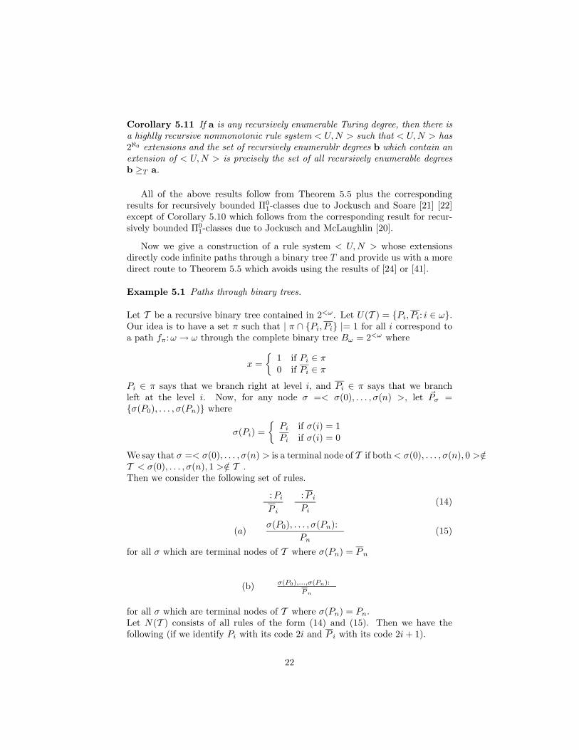
Now we give a construction of a rule system < U,N > whose extensionsdirectly code infinite paths through a binary tree T and provide us with a moredirect route to Theorem 5.5 which avoids using the results of [24] or [41].

Example 5.1 Paths through binary trees.

Let T be a recursive binary tree contained in 2<ω. Let U(T ) = {Pi, Pi: i ∈ ω}.Our idea is to have a set π such that | π ∩ {Pi, Pi} |= 1 for all i correspond toa path fπ:ω → ω through the complete binary tree Bω = 2<ω where

x =

{1 if Pi ∈ π0 if Pi ∈ π

Pi ∈ π says that we branch right at level i, and Pi ∈ π says that we branchleft at the level i. Now, for any node σ =< σ(0), . . . , σ(n) >, let ~Pσ ={σ(P0), . . . , σ(Pn)} where

σ(Pi) =

{Pi if σ(i) = 1Pi if σ(i) = 0

We say that σ =< σ(0), . . . , σ(n) > is a terminal node of T if both< σ(0), . . . , σ(n), 0 >/∈T < σ(0), . . . , σ(n), 1 >/∈ T .Then we consider the following set of rules.

:Pi

P i

:P iPi

(14)

(a)σ(P0), . . . , σ(Pn):

Pn(15)

for all σ which are terminal nodes of T where σ(Pn) = Pn

(b) σ(P0),...,σ(Pn):

Pn

for all σ which are terminal nodes of T where σ(Pn) = Pn.Let N(T ) consists of all rules of the form (14) and (15). Then we have thefollowing (if we identify Pi with its code 2i and P i with its code 2i+ 1).

22

Theorem 5.12 Let T ⊆ 2<ω be a recursive tree.(i) < U(T ), N(T ) > is a highly recursive nonmonotonic rule system and(ii) E is an extension of < U(T ), N(T ) > if and only if the map fE :ω → ωdefined by

fE(i) =

{1 if Pi ∈ E0 if P i ∈ E

is an infinite path through T .

Given Theorems 5.1 and 5.5, it is natural to ask if there are analogous resultsfor locally finite nonmonotonic rule systems which are recursive, but not highlyrecursive. The answer is “yes”. That is, we say that a tree T ⊆ ω<ω is highlyrecursive in 0′ if T is recursive in 0′, T is finitely branching, and there is aprocedure which is recursive in 0′ and which given any node η ∈ T will producethe canonical index of the set of immediate successors of η in T . Then theanalogues of Theorems 5.1 and 5.5 hold for recursive nonmonotonic rule systemsif we replace highly recursive trees by trees which are highly recursive in 0′.

Moreover, by relativization to the code of the collection of rules < U,N > weare able to deal with the case of arbitrary locally finite nonmonotonic system S.The distinction between the form of function that computes the canonical indexof the collection of prooof schemes for elements of U remains, if this functionis recursive in (the code of) < U,N >, then the tree T whose branches codeextensions of < U,N > is recursive in (the code of) < U,N >. Otherwise it isrecursive in its jump.

These results will be proved in a subsequent paper.

5.4 Some applications to Logical Systems

The results of Sections 5.1 and 5.3 can be interpreted, using Sections 3.2 and 3.3,as (new) results about default logic and logic programming. The relationshipbetween stable semantics for logic programs and default logic and the resultsof Section 3.3 show the relevance of proof schemes to the construction of stablemodels for logic programs. As far as we know, programs with the local finite-ness property have not been discussed previously in the literature, although thiscovers most practical programs. The definition of proof scheme with a “forbid-den” set of atoms (corresponding to the definition of support of a proof schemeabove) is perfectly natural and can be lifted from definition (12) in an obviousfashion. The ordering ≺ has the same meaning as before. This way, we get anatural concept of a locally finite (propositional) program. When the programP involves variables, we interpret P as the collection of its Herbrand constantsubstitutions. This gives rise to a definition of locally finite program. The rulesystems of Sections 5.1 and 5.3 can be rewritten following reverse translationsof Section 3.3 (notice that we deal there only with atoms!). That is, the ruleq1,...,qn:r1,...,rm

pis translated to: p← q1, . . . ,¬qn, r1, . . . ,¬rm. Using Proposition

23

3.2 we get stable models from extensions. It is easy to see that the concept ofproof scheme is preserved, locally finite systems generate locally finite programs.Then, in an analogous manner, we introduce the notion of a “highly recursiveprogram” as one that is recursive, locally finite, and for which a function as-signing to p the code of its finite collection of its ≺-minimal proof schemes isrecursive. Let Stab(P ) be the collection of stable models of the program P . Wethen get

Theorem 5.13 Given a highly recursive program P there is a highly recursivetree T ⊆ 2<ω and an effective one-to-one degree preserving correspondence be-tween Stab(P ) and P(T ).

Exactly the same lifting may be done for default logic. We leave the details tothe reader.

So the results of Jockusch and Soare apply both to logic programming and todefault logic, and we get a series of results on recursion theory of stable modelsof logic programs by lifting Corollary 5.2, Theorem 5.5, Corollaries 5.6, 5.7, 5.8,5.9, 5.10, 5.11, and Theorem 5.12.

It is appropriate to compare the results of this section with those of [2]. Theyconstruct, for a given natural number n ≥ 1, a stratified finite program P (inparticular its Herbrand expansion is a recursive propositional program) whoseperfect model is a complete Σ0

n set of natural numbers. Since the perfect modelis stable, and stratified programs possess the unique stable model (as pointed by[10]), the collection Stab(P ) is a one element class. Then this is a Π0

2-class, whoseonly element is a Σ0

n set. Our results show that it is impossible to find a recursiveprogram possessing a unique stable model which is Π1

1-complete; as the uniqueelement of an arithmetical singleton class in 2ω must be hyperarithmetical.

6 Semantics

Let < U,N > be a deductive system and assume that |U | = ω. Without loss ofgenerality we may identify the set U with the set ω of natural numbers, and N ,which consists of finite objects, with a subset of ω.

Let us recall that we wish to characterize three classes: minimal sets closedunder N , weak extensions, and extensions of < U,N >. We shall providea semantic characterization of these concepts. These characterization use theinfinitary logic.

The logic LS is defined as the closure of a collection of atoms of form “ϕ ∈ S”(ϕ ranging over U) under negation, arbitrary denumerable conjunctions andarbitrary denumerable disjunctions.

Given T ⊆ U , and ϕ a formula of LS , define the satisfaction relation T |= ϕ

24

by induction in the most natural fashion:(1) T |= α ∈ S if and only if α ∈ T .(2) T |= ¬ψ if and only if not(T |= ψ).(3) T |=

∧∧i∈J ψi if and only if for all i ∈ J , T |= ψi.

(4) T |=∨∨i∈J ψi if and only if there exists i ∈ J , such that T |= ψi.

The connectives ⇒ and ⇔ are abbreviations.Associate with each rule:

r =α1, . . . αn:β1, . . . , βm

ϕ(16)

a finitary formula of LS ,

t(r) = [α1 ∈ S ∧ . . . ∧ αn ∧ ¬(β1 ∈ S) ∧ . . . (17)

∧¬(βm ∈ S)]⇒ ϕ ∈ S.The object ϕ is denoted by c(r).

Proposition 6.1 A subset T of U is deductively closed if and only if for allr ∈ N , T |= t(r).

Generalizing Clark’s completion from logic programming, we define “Clark’scompletion” of a deductive system < U,N >. This is a theory in LS , possiblyinfinitary. To define it, assume that r is a rule of form (16). Set

A(r) = α1 ∈ S ∧ . . . ∧ αn ∈ S ∧ ¬(β1 ∈ S)∧ (18)

. . . ∧ ¬(βm ∈ S).Thus t(r) = Ar ⇒ (c(r) ∈ S). Now, given α ∈ U , let Fα be

α ∈ S ⇔∨∨{Ar: r ∈ N ∧ c(r) = α ∈ S} (19)

Fα says that α belongs to T exactly if it is supported by a formula of the formAr for some r ∈ N .

The formulas Fr can be used to characterize weak extensions.

Theorem 6.2 A collection T ⊆ U is a weak extension of < U,N > if and onlyif for all α ∈ U , T |= Fα.

Now, identifing U with the set of natural numbers ω, the collection of allsubsets of U is identified with 2ω, this is the Cantor space. Then:

Proposition 6.3 For every formula Φ ∈ LS, {T :T |= Φ} is a Borel subclassof 2ω in the Cantor topology.

Corollary 6.4 (a) Let < U,N > be a deductive system, U = ω. The collectionW of weak extensions of < U,N > is a Borel subclass of 2ω.(b) Consequently, |W | is finite, or |W | = ω or |W | = 2ℵ0 .

25

When < U,N > is recursive, then the formula∨∨{Ar:ψ = c(r)} is representable

as a recursively enumerable set of natural numbers. it follows that:

Proposition 6.5 If < U,N > is recursive, then the collection of weak exten-sions of < U,N > is a Π0

2 subclass of 2ω.

The collection of all extensions of a deductive system has a model-theoreticalcharacterization. Using the idea behind proof schemes we can introduce aninfinitary description of provability. Fix < U,N >.

Proposition 6.6 For every ψ ∈ U there exists a formula prψ ∈ LS such thatfor every T ⊆ U , T |= prψ if and only if ψ possesses a T -derivation. (prψdepends on N)

Corollary 6.7 Let < U,N > be a deductive system. Then T ⊆ U is an exten-sion of < U,N > if and only if:(1) For all ψ ∈ T , T |= prψ, and(2) For all ψ /∈ T , T |= ¬prψ.

Corollary 6.8 (a) Let < U,N > be a deductive system, U = ω. The collection

E of extensions of < U,N > is Π0,N2 subclass of 2ω.

(b) Consequently, |E| is finite, or |E| = ω or |E| = 2ℵ0 .

6.1 Applications in Default Logic and Logic Programming

Proposition 6.9 Let < D,W > be a default theory. < U,N > be its trans-lation as a nonmonotonic rule system, and let S be a subset of U satisfyingtranslation of < D,W >. Then:(1) S is a weak default extension of < D,W > if and only if for all ϕ ∈ L,S |= Fϕ.(2) S is a default extension of < D,W >if and only if:(i) for all ϑ ∈ S, S |= prϑ.(ii) for all ϑ /∈ S, S |= ¬prϑ.

Compare this result with the earlier results of Etherington ([9]) who char-acterized default extensions by means of “most preferred models”. Here we usea different device. A careful inspection of our method indicates the following:First, imbed the language L into a new language LS . This language LS pos-sesses a new atom for every formula of L. Thus, LS is a much richer language.Second, formulas of L are translated as atoms of LS . The relationship betweenvarious formulas of L is enforced in LS by means of translations of rules. Defaultrules of L are translated to certain finitary clauses of LS . Checking satisfaction

26

for these clauses refers only to simpler formulas of LS . Some of these are notimages of formulas of L. The semantic characterization of extensions and weakextensions refers to formulas of LS which are not images of formulas of L. Inaddition, these formulas used in characterization are infinitary. This indicatesan infinitary character of the concept of extension and weak extension.

One needs to notice that when the theory < D,W > is finite, our descriptionof it, via the translation to nonmonotonic rule systems is finitary. Also, thecharacterization formulas prψ are finitary. The reason for this is that, in additionto rules in D, we also have all the rules of logic. The schemes of proof oflogic result in infinitely many rules which are, however, monotonic. There areinfinitely many proof schemes, but the collection of formulas of form k(p) isfinite anyway! This fact results in the finitary algorithm described in [25].

Our translation of propositional logic programs as rule systems provides uswith an infinitary characterization of stable models of logic programs. Thereason this is important is that the definition of stable model of logic program,as introduced in [10], is purely operational. Let P be a logic program, Π itspropositional version, that is the collection of all the Herbrand substitutions ofP . Let H be the Herbrand base of P and let M ⊆ H. Gelfond and Lifschitzgive an algorithm for testing whether M is stable structure for P and provethat a stable structure is, actually, a minimal model of P . It should be clearfrom this description that this definition is purely operational. Here, using theinfinitary language LS we give a purely logical, although infinitary, descriptionof stability.

Proposition 6.10 Let P be a logic program, Π its propositional version, H,Herbrand base of P , and finally < H,T > the translation of Π described inSection 3.3. Then M ⊆ H is a stable model of P if and only if for everyϑ ∈ M , ϑ is M -derivable in < H,T >. and for every ϑ /∈ M , ϑ is not M -derivable in < H,T >.Thus M ⊆ H is a stable model of P if and only if(i) for every ϑ ∈M , M |= prϑ.(ii) for every ϑ /∈M , M |= ¬prϑ.

7 Conclusion

In a sequel we deal with rule systems containing variables in the rules. Weshall deal with predicate logics. We shall prove results related to the propertiesof recursive systems that are not necessarily highly recursive. We also exploreconnections with Lω1,ω.

We acknowledge helpful conversations and discussions with Krzysztof Apt,Howard Blair, Michael Gelfond, John Schlipf, V.S. Subrahmanian, and MiroslawTruszczynski.

27

References

[1] K.R. Apt. Introduction to Logic Programming. TR-87-35, University ofTexas, 1988.

[2] K.R. Apt, H.A. Blair. Classification of Perfect Models of Stratified Pro-grams. To appear in Fundamenta Informaticae.

[3] K.R. Apt, H.A. Blair, A. Walker. Towards a theory of declarative knowl-edge. In: J. Minker ed. Foundations of Deductive Databases and LogicProgramming, pp. 89-142, Morgan Kaufmann, Los Altos, CA.

[4] N. Bidoit, C. Froixdevaux. General logical databases and programs, de-fault logic semantics, and stratification. J. Information and Comput., toappear.

[5] H.A. Blair, A.L. Brown, V.S. Subrahmanian. Monotone Logic Program-ming. Technical Report CS-TR-2375, University of Maryland.

[6] J. de Kleer. An Assumption-based TMS. Artificial Intelligence 28:127 –162, 1986.

[7] R.P. Dilworth. A decomposition theorem for partially ordered sets. Annalsof Mathematics 51 (1950) pp. 161-165.

[8] J. Doyle. A Truth Maintenance System. Artificial Intelligence Journal12:231–272, 1979.

[9] D.W. Etherington. Formalizing Nonmonotonic Reasoning Systems. Arti-ficial Intelligence Journal 31:41–85, 1987.

[10] M. Gelfond, V. Lifschitz. Stable Semantics for Logic Programs. In: Pro-ceedings of 5th International Symposium Conference on Logic Program-ming, Seattle, 1988.

[11] M. Gelfond, V. Lifschitz. Logic Programming with Classical Negation.Unpublished Manuscript.

[12] M. Gelfond, H. Przymusinska. On the Relationship between Circumscrip-tion and Autoepistemic Logic. In: Proceedings of the ISMIS Conference,1986.

[13] M. Gelfond, H. Przymusinska. Inheritance Reasoning in AutoepistemicLogic, Manuscript, 1989.

[14] D. Gries. The Science of Programming. Springer-Verlag 1981.

[15] P. Hall On representatives of subsets. Journal of London MathematicalSociety 10 (1935) pp. 26-30.

28

[16] M. Hall. Distinct representatives of subsets. Bulletin of American Math-ematical Society 54 (1948), pp. 922-926.

[17] J.Y. Halpern, Y.O. Moses, Knowledge and Common Knowledge in aDistributed Environment, 3rd ACM Conference on the Principles of Dis-tributed Computing, pp. 50-61.

[18] J. Hintikka Knowledge and Belief. Cornell University Press.

[19] W-Q. Huang, A. Nerode. Applications of Pure Recursion Theory to Re-cursive Analysis. Acta Sinica 28.

[20] C.G. Jockusch, T.G. McLaughlin. Countable retracing functions and Π02

predicates. Pacific Journal of Mathematics 30 (1972) pp. 69-93.

[21] C.G. Jockusch, R.I. Soare. Π01 classes and degrees of theories. Transactions

of American Mathematical Society 173 (1972) pp. 33-56.

[22] C.G. Jockusch, R.I. Soare. Degrees of members of Π01 classes. Pacific

Journal of Mathematics 40 (1972) pp. 605-616.

[23] K. Konolige. On the Relation between Default and Autoepistemic Logic.Artificial Intelligence 35:343–382, 1988.

[24] A. Manaster, J. Rosenstein. Effective matchmaking. Proceedings of theLondon Mathematical Society 25 (1972) pp. 615-654.

[25] W. Marek, A. Nerode. Decision procedure for default logic MathematicalSciences Institute Reports, Cornell University.

[26] W. Marek, V.S. Subrahmanian. The Relationship Between Logic ProgramSemantics and Non-Monotonic Reasoning. In: Proceedings of the FifthInternational Conference on Logic Programming, M.I.T. Press.

[27] W. Marek and M. Truszczynski. Autoepistemic Logic, to appear.

[28] W. Marek and M. Truszczynski. Relating Autoepistemic and Default Log-ics. In: Principles of Knowledge Representation and Reasoning, MorganKaufman, San Mateo, 1989. (Full version available as Technical Report144-89, Computer Science, University of Kentucky, Lexington, KY 40506-0027, 1989.)

[29] W. Marek and M. Truszczynski. Stable models for logic programs anddefault logic. In: Proceedings of North American Conference on LogicProgramming, MIT Press, 1989. (Full version available as Technical Re-port, Computer Science Department, University of Kentucky, Lexington,KY 40506-0027, 1989.)

[30] J. McCarthy. Circumscription — a form of non-monotonic reasoning.Artificial Intelligence Journal, 13:27–39, 1980.

29

[31] G. Metakides, A. Nerode. Effective Content of Field Theory. Annals ofMathematical Logic, 17:289–320.

[32] M. Minsky. A framework for representing knowledge. In: The Pychologyof Computer Vision, pp.211-272. McGrow Hill.

[33] L. Mirsky. Transversal Theory. Academic Press, New York.

[34] R.C. Moore. Semantical Considerations on Non-Monotonic Logic. Artifi-cial Intelligence, 25:75–94, 1985.

[35] A. Nerode, J.B. Remmel. A Survey of r.e. Substructures. Proc. Symp.Math. 42, Amer. Math. Soc.

[36] A. Nerode, J.B. Remmel. Complexity-theoretic Algebra I: Vector Spacesover Finite Fields. In: Structures in Complexity. pp. 218-241.

[37] A. Nerode, J.B. Remmel. Complexity-theoretic Algebra II: Boolean Al-gebras. Annals of Pure and Applied Logic 44:71–99.

[38] A. Nerode, J.B. Remmel. Complexity-theoretic Algebra III: Bases of Vec-tor Spaces. In: Feasible Mathematics, Springer Verlag.

[39] M. Reinfrank, O. Dressler. On the Relation between Truth Maintenanceand Non-Monotonic Logics. In: Proceedings of International Joint Con-ference on Artificial Iintelligence, 1989.

[40] R. Reiter. A Logic for Default Reasoning. Artificial Intelligence, 13:81–132, 1980.

[41] J.B. Remmel. Graph colorings and recursively bounded Π01 classes. Annals

of Pure and Applied Logic 32 (1986) pp. 185-194.

[42] J.B. Remmel. Recursive Boolean Algebras. In: Handbook of BooleanAlgebras

[43] A. Tarski. Logic, Semantics, Metamathematics Oxford, 1956.

30