signaling, free cash flow, and “nonmonotonic” dividends · signaling, free cash flow, and...

1

SIGNALING, FREE CASH FLOW, AND “NONMONOTONIC” DIVIDENDS

Kathleen Fuller Terry College of Business, University of Georgia, Athens, GA 30602

Anjan Thakor University of Michigan Business School, Ann Arbor, MI 48109

This Draft: June 14, 2002

Corresponding author: Anjan Thakor, 701 Tappan St., Ann Arbor, MI 48109, (734) 647-6434. Email: [email protected]

Acknowledgements: We would like to thank Jeff Bacidore, Marc Lipson, seminar participants at the University of Georgia, Michael Fishman (the editor) and two anonymous referees for valuable comments.

2

Abstract

It has long been argued that dividends are used as a signal of future earnings or as a means of distributing excess cash. However, the empirical tests of these two hypotheses have generated inconclusive results. One reason for these inconclusive results is that no model combines both the signaling and cash-flow-distribution aspects of dividends. This paper develops a framework in which firms have an incentive to pay dividends to both signal and distribute free cash flows. High-quality observationally-distinct firms pay dividends to eliminate the free-cash-flow problem, while high-quality observationally-similar firms that the market perceives as intermediate quality pay dividends to both signal future earnings and reduce the free-cash-flow problem. The equilibrium entails a nonmonotonicity in dividend payments with respect to the signal observed by the market at the interim date; the highest quality firms pay lower dividends than those of intermediate quality. Our theoretical argument helps reconcile the existing inconclusive empirical findings and also generates new empirical predictions that are then tested. The evidence supports these predictions.

SIGNALING, FREE CASH FLOW, AND “NONMONOTONIC” DIVIDENDS

I. INTRODUCTION

Why does a firm pay dividends? This question, which we study here, has been the subject of

debate for many years, dating back to the pre-Miller and Modigliani (1961) era when it was believed that

increasing dividends would always increase market value. Miller and Modigliani showed that, under

certain conditions, dividend policy is irrelevant to firm value. Since then, many arguments have been

proposed to rationalize why dividends matter. Maybe firms pay dividends to attract certain clienteles, or

maybe to signal some information to the market, or maybe just to return excess cash fairly to all

shareholders. As of yet, no single theory has become dominant. This is perhaps because there are

multiple motivations for paying dividends and there is not one single reason that applies to all firms.

Though research has proven rather convincingly that there is little evidence of a clientele effect for firms

paying dividends, the empirical contest between the signaling and excess-cash hypotheses continues to

this day. 1

The dividend-signaling hypothesis suggests managers with better information than the market

will signal this private information using dividends. Bhattacharya (1979), John and Williams (1985),

Miller and Rock (1985), and Ofer and Thakor (1987) all develop signaling models in which either taxes

or distress borrowing costs create a dissipative cost that makes dividends a credible signal. The excess-

cash hypothesis suggests that since managers cannot credibly precommit to shareholders that they will not

invest excess cash in negative-NPV projects, dividend changes may convey information about how the

firm will use future cash flows. Easterbrook (1984), Jensen (1986), and Lang and Litzenberger (1989) all

suggest that increasing dividends ensures that there is less free cash flow available to be wasted on

inefficient projects, perks, and the like. The empirical implication from both hypotheses is that firms that

increase (decrease) dividends should have positive (negative) price reactions. Indeed, dividend changes

have been documented to generate significant stock price reactions.

1 See the excellent review article by Allen and Michaely (2002) for a thorough discussion of the theory and the evidence.

2

While at a general level both these explanations for why firms pay dividends appear to have

empirical merit, bothersome gaps between the theories and the data begin to appear upon closer

inspection. Consider the signaling hypothesis first. Its strongest prediction is that there is a monotonic

relation between unexpected dividend changes and new information about future earnings acquired by the

manager. This means that future earnings should be strictly increasing in dividend increases. This

prediction is typically generated in a static model in which there are firms that are a priori observationally

identical to the market but have different levels of future earnings about which the managers of these

firms are privately informed. Thus, what one needs to test is a cross-sectional relation. This is difficult

because it requires the empiricist to disentangle what the manager was privately informed about at the

time of the dividend signal from what the whole market knew, i.e., determine the set of firms that were

observationally identical to the market. Perhaps this is why the empirical evidence on the signaling

hypothesis seems inconclusive.

As Allen and Michaely (2002) point out, the evidence supportive of the signaling hypothesis

indicates that dividend changes are associated with changes in stock price of the same sign around the

dividend change announcement and the immediate price reaction is related to the magnitude of the

dividend. However, the overall empirical evidence is not very supportive of traditional signaling models

because of two sets of findings. First, the relation between dividend changes and subsequent earnings

changes are inconsistent with the theory; it appears that dividends are related more strongly to past

earnings than future earnings (e.g., Benartzi, Michaely, and Thaler (1997)). Second, there is a significant

price drift in subsequent years and, perhaps suggestive of the free-cash-flow hypothesis, it is the large and

profitable firms (with less informational asymmetries) that pay most of the dividends (e.g., Fama and

French (2001)).

Allen and Michaely (2002) discuss similarly mixed evidence about the free-cash-flow (FCF)

hypothesis. For example, Grullon, Michaely and Swaminathan (2002) find that firms anticipating

declining investment opportunities are likely to increase dividends and Lie (2000) found that firms that

increased dividends had cash in excess of that held by peer firms in the industry. These papers thus

3

provide evidence supportive of the FCF hypothesis. However, Yoon and Starks (1995) found a

symmetric price reaction to dividend changes across high-Tobin’s Q and low-Tobin’s Q firms, which

goes against the FCF hypothesis. Overall, there appears to be more empirical support for the FCF theory

than for signaling, but the somewhat inconclusive nature of the evidence makes it hard to pick a definite

winner.

Perhaps one reason for the mixed empirical evidence is that we lack an integrated theory that

incorporates both the signaling and FCF motivations for dividends. Our goals in this paper are twofold.

The first is to develop a simple argument that ties together the signaling and FCF motives to pay

dividends. This argument helps understand the inconclusive empirical evidence a bit better and also

generates additional testable predictions. Second, we test these additional predictions.

In the argument we develop, a promised dividend payment represents a precommitment to pay

out a certain amount of cash.2 This precommitment can be either to signal the manager’s private

information about future cash flow when the market is unaware of it or to simply disgorge excess cash to

minimize value dissipation due to the FCF problem, even when the manager and the market are

symmetrically informed about future cash flow. As is standard in discrete signaling models, we stipulate

two types of observationally-identical firms, good and bad, each with a different future cash flow. Based

on observed financial performance, the market then generates a noisy signal about each firm’s type prior

to the realization of the future cash flow. The signal leads to three observationally-distinct types of firms:

(1) good firms correctly identified as such because the signal takes a high value, (2) good and bad firms

lumped together in the same group because the signal takes an intermediate value and does not distinguish

between them, and (3) bad firms correctly identified as such because the signal takes a low value.

The core intuition behind our analysis rests on the joining together of two simple ideas. One is

that informational asymmetry about a firm’s future prospects is likely to be the greatest when its observed

2 The best way to view our argument is as one in which, like most other dividend theories, a dividend is presumed to be the best way to deal with either a signaling or a FCF problem, and the issue is the level of dividends needed to solve the problem. A more ambitious goal would be to build a model that comprehensively treats dividends as one of many mechanisms to deal with these problems. Such an exercise is not our objective.

4

performance is relatively ambiguous, neither good nor bad, but investors realize that these firms represent

a mixed bag of good and bad firms. The other is that the FCF problem is the most severe when the firm’s

performance is good and it has generated relatively high cash flow. Pasting these two ideas together

makes the possibility of nonmonotonic dividend equilibria arise rather naturally. The identifiably bad

firms (group (3)) pay low dividends because there is no informational asymmetry about them and they

have relatively low “free cash” to disgorge. The identifiably-good firms (group (1)) pay dividends, but to

reduce the severity of the FCF problem rather than to signal. Finally, the good firms with the ambiguous

financial performance (group (2)) pay the highest dividends because they need to signal in order to

distinguish themselves from the observationally-identical bad firms in group (2), and they also need to

deal with the FCF problem.

The equilibrium thus entails a nonmonotonicity in dividend payments with respect to the signal

observed by the market at the interim date; the highest quality firms pay lower dividends than those of

intermediate quality. In a standard signaling equilibrium, higher-quality types distinguish themselves

from lower-quality types by emitting a signal of greater magnitude. This occurs because the signal chosen

for the game is the only instrument by which the higher-quality types can separate themselves. By

contrast, in our framework, the high-quality types can avail of other (possibly costless) mechanisms –

such as past performance – to separate themselves, so type-dependent signaling is restricted to a subset of

types.

The nonmonotonicity of the equilibrium is important for the following reason. If one views

monotonicity as an essential ingredient of a signaling equilibrium, as is the case with the standard

signaling model, then one risks empirically rejecting the signaling explanation for dividends because the

data are inconsistent with monotonicity, even when dividend signaling may have empirical merit. In

addition to providing this perspective on the existing evidence, our approach generates the following main

testable predictions.

• Firms that have had poor prior performance will pay the lowest dividends and will have little

heterogeneity among themselves in future earnings.

5

• Firms that have had good prior performance will pay high dividends to protect against losses due to

the FCF problem but will also have little heterogeneity among themselves in future earnings.

• Firms with moderate prior performance will pay the highest dividends and have the highest

intragroup heterogeneity in current dividend payments as well as future earnings.

• Firms with good prior performance will have a positive abnormal price reaction to the dividend

increase. However, the price reaction will be less than that for firms with moderate prior

performance.

These predictions are tested using a sample of firms with regular quarterly dividend payments

between 1980 and 2000. We find that firms with moderate past performance pay significantly larger

dividends and have higher unexpected future earnings compared to those with poor or good past

performance. Also, firms with moderate past performance have greater variability among themselves –

reflecting greater intragroup heterogeneity – in dividends and future earnings as compared to firms with

poor or good past performance. Finally, we find that the abnormal price reaction associated with dividend

increases for firms with moderate performance is significantly larger than that for firms with good past

performance.

The remainder of the paper is organized as follows. Section II presents the theoretical arguments.

Section III lists the testable predictions discussed above and describes the empirical tests and results.

Section IV concludes.

II. THE THEORETICAL ARGUMENT

In this section, we lay out the theoretical argument that motivates our empirical analysis.

Although it is possible to present a formal model along these lines, we simply present the main idea

verbally because it suffices to generate testable predictions.

There is universal risk neutrality and the risk free rate is zero. Suppose there are innately two

types of firms: G (good quality) and B (bad quality), with a commonly-known prior distribution over

types. A good-quality firm has two possible future cash flows (CFs): H or L where H > L > 0. A bad-

quality firm has two possible future CFs: L or 0. Let x represent the CFs, then Pr (x = H|G) = q,

6

Pr (x = L|G) = 1 – q, Pr (x = L|B) = q, and Pr (x = 0|B) = 1 – q. Future CFs are realized at time t=2 and

observed by all. At time t=1, there is a signal, s, that outsiders observe that conveys additional

information about the cash flows at t=2. Think of s as informative signal produced by the union of the

firm’s past performance (prior to t=1) and additional interim performance information – such as an

interim earnings report – that may become available at t=1. The signal can take one of three values, 0, L,

or H. If the firm is G, then s ∈{L, H} and if the firm is B, then s ∈ {0, L}. The probability distribution

of s is given by: Pr(s=H|G) = q, Pr(s=L|G) = 1-q, Pr(s=0|G) = 0, Pr(s=H|B) = 0, Pr(s=L|B) = q, and

Pr(s=0|B) = 1-q. Note there is no correlation (by assumption) between the s observed at t = 1 and the

CF(x) at t = 2, conditional on the firm’s type; unconditionally, s and x are correlated through firm type.

Also at t=1, the manager observes his firm’s true type. After the market receives its signal s , the manager

announces at t=1 the dividend the firm will pay at t=2. We assume, for simplicity, that the previous

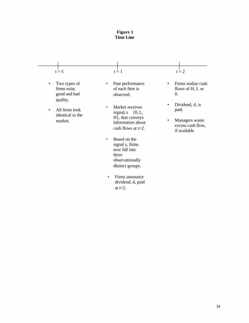
dividend level was zero, so any dividend d>0 at t=1 represents a dividend increase. Figure 1 indicates the

time line of the model.

Insert Figure 1

Therefore, at t = 1 there are three observationally distinct types of firms the market sees prior to

observing the firm’s dividend choice:

1. Firms for which s = H is observed by outsiders. These firms are identified correctly as G with

probability 1.

2. Firms for which s = L is observed. These firms could be either G or B.

3. Firms for which s = 0 is observed. These firms are identified correctly as B with probability 1.

If the firm promises to pay a dividend and its cash flow falls short of the promised dividend, d,

we assume that it will need to make up the difference by external borrowing that carries a cost ( )c i that

exceeds the riskfree rate of zero, i.e., the firm will incur a dissipative financing cost of c(d(x)), where x is

the realized cash flow, d(x) = max {d – x, 0}, ( )( )c d 0,x′ > ( )c 0,′′ >i and c(0) = 0. Thus, the cost ( )c i is

relevant when d>x. Moreover, if x>d, then the firm faces a FCF problem in that, due to the personal

7

benefits of overinvesting, those below the manager (call them “junior managers”) will engage in wasteful

(negative NPV) investments, with a loss in value of ( )Ψ i . Hence, the loss in value due to the FCF

problem is ( )ˆ(d)Ψ x where { } ( ) ( )ˆ(d) max d,0 , 0, 0,x x ′ ′′= − Ψ > Ψ >i i and ( )0 0.Ψ = Whether the

manager will wish to eliminate such overinvestment by the junior managers depends on whether he

himself has any personal benefits associated with overinvesting. Let γ∈(0,1) be the probability that the

manager does not personally benefit from overinvestment. Hence, the probability that the manager will

eliminate the FCF problem is γ. The manager here should be viewed as the CEO, who may or may not be

interested in stopping the wasteful behavior of those below him in the organization. The role of γ is to

ensure that there is some valuation-relevant residual uncertainty for all firms even though firms fall into

observationally-distinct groups based on prior performance. The promise of a dividend will help resolve

this uncertainty even when there is no heterogeneity in innate firm values within a group of

observationally-identical firms.

The idea behind the FCF problem described above is that the CEO may have the strongest

preference for maximizing shareholder value among all employees in the firm. This may be because the

CEO’s compensation is the most sensitive to the firm’s stock price and/or because he faces the greatest

direct pressure from institutional shareholders to attend to shareholder value. When there is cash lying

around, the CEO will wish to invest it in positive-NPV projects. Lower-level employees (junior

managers) may also want to do this when positive-NPV projects are available. However, in the absence

of such projects, they may still wish to request project finding for a variety of reasons. One reason is that

relative status within the firm may depend on the resources the junior manager controls, so junior

managers try to acquire capital even if it means dressing up negative-NPV projects as good projects. The

other is that the project may actually be good for the junior manager’s division but it expropriates value

from other divisions, so that the overall NPV for the firm is negative. Consequently, the propensity to

engage in inefficient investments is likely to be stronger at levels below the CEO, and the CEO’s ability

to control this directly may be hampered by asymmetric information. If this is the case, the CEO may not

8

only want to precommit to funding projects only out of internal cash flows but also precommit to paying

dividends to reduce the amount of FCF left over for junior managers to invest in their “pet” projects. Of

course there is no guarantee that the CEO will never derive any personal benefit from such

overinvestment, which is what the parameter γ captures.

We now have sufficient structure to extract implications. Consider first the firms in group 1.

Since these firms are correctly identified as G firms by investors, there is no signaling motivation to pay

dividends. However, these firms expect a cash flow of either H or L at t=2 and hence may wish to set a

dividend, say 1Gd , to resolve the FCF problem and avoid the cost ( )Ψ i . Note that setting 1

Gd H= would

eliminate the FCF problem entirely, but will not necessarily be optimal because the firm will incur a

dissipative external financing cost of c(H-L) if x=L. There is thus a tradeoff between the costs ( )c i and

( )Ψ i , and we cannot pin down exactly what 1Gd will be without an explicit formal analysis. There

should, however, be a positive stock price reaction to the announcement of 1Gd because it signals to the

market that the manager does not himself derive a personal benefit from overinvesting, i.e., the market’s

posterior belief that the manager has no private benefit from overinvesting goes from γ to 1.

Now consider the firms in group 3. They too have no signaling motive because they are correctly

identified by investors. Everybody knows at t=1 that a firm in this group will have a cash flow of L or 0

at t=2. The only reason for promising a dividend at t=1 is to reduce/eliminate the FCF problem and the

associated cost ( )Ψ i . Let 3Bd be the dividend that achieves this. Because the expected future cash flow

of a group-3 firm is smaller than that of a group-1 firm, we expect that the respective tradeoff between the

costs ( )c i and ( )Ψ i will lead to 3 1B Gd d< . The announcement effect of the dividend will be smaller than

that for group-1 firms because the potential gain from eliminating the FCF problem is smaller.

Finally, consider the group-2 firms. There are G and B firms in this group but the market views them

as observationally identical. This is the most heterogeneous of the three groups. The B firms will, in

9

equilibrium, set their dividend, 2Bd , to solve their FCF problem, i.e., 2 3

B Bd d .= The G firms, by contrast

still choose a dividend of at least 1Gd to solve their FCF problem. However, they will also need to ensure

that their dividend is high enough to deter the B firms from mimicking them. Let sGd be the dividend

level that achieves this signaling outcome. While it is possible for s 1G Gd d ,< in which case 1

Gd will be the

chosen dividend level, it is not difficult to find conditions under which s 1G Gd d .> In this case, the G firms

in group 2 will choose sGd . In general then, if we define { }2 1 s

G G Gd max d ,d= as the level of dividends

chosen by G firms in group 2, we can say 2 1G Gd d ,≥ and in special cases (i.e., if signaling incentive

compatibility is a binding constraint), we have 2 1G Gd d .>

By joining together three ideas – signaling, FCF and observably distinct firms types – we can thus

generate an equilibrium in which the relationship between dividends and observable firm quality could be

nonmonotonic. Firms with moderate past performance may pay the highest dividends, followed by those

with the best performance, and finally the firms with the worst performance.

III. EMPIRICAL PREDICTIONS AND TESTS

The theoretical argument has several new empirical predications not generated by the standard

signaling models or FCF models. In what follows, we refer to the prior performance of firms in group 1

as "good", firms in group 2 as "moderate", and firms in group 3 as "poor". These labels should not be

interpreted literally. The firms classified as "poor" are not necessarily firms with poor prior performance

in an absolute sense. Rather, among firms that either increased their dividends or kept them the same,

these firms had the poorest relative performance.3

3 In the empirical tests that follow, it would be tempting to include firms that cut dividends since such firms seem to be ideal candidates for being classified as poor. However, our framework does not include dividend-reducing firms, so we exclude these from the sample.

10

A. The Predictions

Hypothesis A: Firms that have had poor prior previous performance will pay the lowest dividends and

will have less heterogeneity in future earnings among themselves relative to the intragroup heterogeneity

among the firms with moderate performance.

As indicated in the theoretical reasoning, managers of firms with poor performance (type-B firms

with s = 0) have already been (correctly) identified as type B firms, so they pay a dividend only to resolve

their FCF problem, and this is the lowest dividend. Further, since these firms have s = 0, it is common

knowledge that x = L with probability q and x = 0 with probability (1-q). Thus, the heterogeneity in

future earnings among firms in this group is low. However, for moderate-performance firms (those with s

= L), we know x ∈ {H, L, 0}. In this group, x = H occurs only when the firm is G, x = L if the firm is

either G or B, and x = 0 only happens when the firm is B. The intragroup heterogeneity in this group is

greater than for the firms with poor prior performance.

At first blush, Hypothesis A looks no different from the prediction of the standard signaling

model that low-quality firms do not signal. One aspect that makes this hypothesis different, however, is

that it refers to firms that are observationally distinct from other firms. The other difference is that this is

a hypothesis about predicted levels of intragroup earnings heterogeneity among the poor-performance

firms and the moderate-performance firms. This is an issue not addressed in the standard signaling

model.

Hypothesis B: Firms that have had good prior performance will pay dividends to protect against losses

due to the FCF problem but will also have less heterogeneity in future earnings among themselves

compared to the intragroup heterogeneity among firms with moderate prior performance.

We argued earlier that firms with good performance have an incentive to pay dividends so to

mitigate the FCF problem. Further, since all of these firms are G, they also have less intragroup

heterogeneity in their future earnings, compared to the heterogeneity among firms with moderate prior

performance.

11

The novelty of this hypothesis is the linking of the prior performance of firms within an

observationally identical group to the intragroup heterogeneity in future performance. We know of no

previous study that has done this.

Hypothesis C: Firms with moderate performance will have the highest intragroup heterogeneity in

current dividend payments and past and future earnings compared to any other group.

This prediction is a direct consequence of the fact that the moderate -performance group has both

B and G firms. The range of dividend payments across moderate-performance firms is larger than for

firms with poor or good prior performance because dividends are serving to signal as well as resolve FCF

problems in the moderate-performance group and only solving the FCF problem in the group consisting

of firms with poor and good performances. Further, past and future earnings should also have the greatest

heterogeneity across the moderate-performance firms since both type-G and type-B firms are combined in

this group. Thus, future cash flows can be H, L or 0 for the moderate -performance firms, while they can

only be H or L for firms with good prior performance, and only L or 0 for the poor-performance firms.

This is perhaps the most novel prediction of our argument.

Hypothesis D: The cumulative abnormal returns (CARs) associated with the announcement effects of

dividends will display greater intragroup heterogeneity for the moderate -performance firms than for

either the good-performance or poor-performance firms.

Note that firms with moderate-prior performance include the G firms that choose dividend 2Gd

and the B firms that choose 2 3B Bd d .= Given that the market views firms in this group as observationally

identical, the dividend announcement effect will be positive in response to 2Gd and negative in response to

2Bd , creating high intragroup variance in the CARs for this group. By contrast, the other two groups are

more homogenous in terms of chosen dividends and hence CARs.

Hypothesis E: While the relative price reactions to dividend announcements will be monotonically

increasing in the size of the dividend increase, the dividend increase itself will not necessarily be

monotonic in observed firm quality.

12

Existing signaling models predict that the larger the dividend change, the larger the price reaction,

and the empirical evidence supports this predictions.4 What is different about our hypothesis is the

statement that the dividend increase will not be monotonic in observed firm quality.

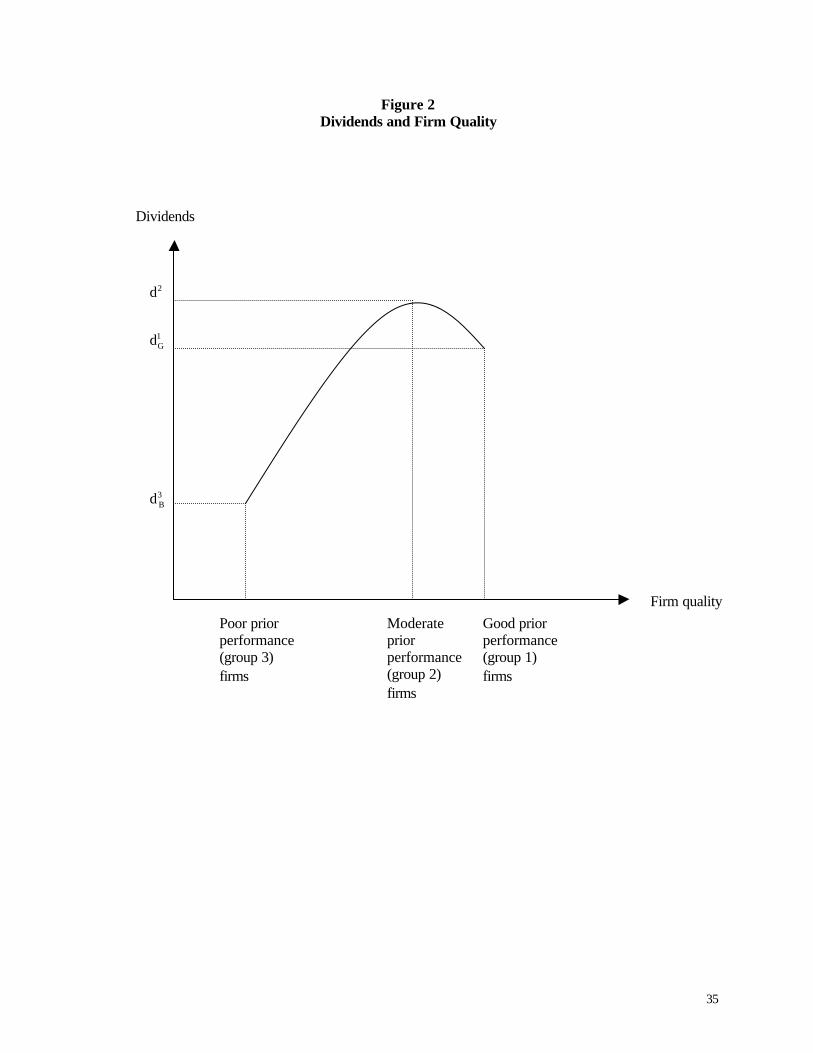
If the fraction of G firms in the moderate-performance group is sufficiently high and the

signaling-driven dividend level ( 2Gd ) sufficiently above that needed to only resolve the FCF problem in G

firms ( 1Gd ), then it is possible for the cross-sectional average of 2

Gd and 2Bd (or 3

Bd ) to be above 1Gd . Let

2d represent the average dividend paid by firms in group 2, so it is possible to have 2 1Gd d> . The

relationship between dividends and firm quality will then look like that in Figure 2.

Insert Figure 2

B. The Data

We confront these predictions with data on dividend-paying firms from 1980 through 2000. The

sample of dividend-paying firms is identified from the Center for Research in Security Prices (CRSP)

daily master file. For a firm to be included in the sample, the following criteria must be satisfied:

i) The dividend increase must be associated with a regular quarterly U.S. cash dividend per share.

ii) The announcement does not represent a dividend initiation or the first dividend since a dividend

omission.

iii) A stock split or stock dividend does not occur in the month before or the month after the dividend

change announcement is made.

iv) Daily return data for the 360 trading days surrounding the dividend announcement are available

from the CRSP daily return file.

v) The firm is listed on the Compustat Quarterly database.5

4 See Allen and Michaely (2002). This is a natural extension of the two-firm-type case to the multi-firm-type case in which all types are separating from each other. 5Though we access all Compustat files (including the research file), our sample will be biased towards large firms since generally Compustat covers larger, more established firms. However, to the extent that Compustat biases our sample, so does our restriction that firms must pay dividends; these will tend to be large firms as well. Thus, any biases introduced by Compustat should be similar to our restriction that firms pay dividends.

13

The first two restrictions ensure that the firms in the sample have paid regular dividend payments

and allow testing of the firm's choice of dividend increase. Restriction iii) is made to control for the

impact stock splits or stock dividends would have on the firm's return during the estimation period.

Restriction iv) allows us to estimate the cumulative abnormal returns for the firms, while restriction v)

ensures we can collect quarterly earnings data as well as other accounting data. Given these restrictions

our final sample is 1,924 NYSE, AMEX, and NASDAQ listed firms with 10,504 dividend increases.6

In designing the empirical tests we wish to undertake, we first classify firms based on prior

performance and then examine dividend payments and past and future earnings changes for the different

groups of firms. To measure the prior performance of the firms, we estimated the cumulative abnormal

returns (CARs), average returns, and buy-and-hold abnormal returns (BHARs) for the firms for 150 days

prior to one month before the dividend announcement. We chose to measure prior performance as stock

performance prior to the dividend announcement since this would incorporate the market’s expectation of

the firm’s future performance. We calculate both CARs and BHARs since the literature is divided on

which specification is best. Fama (1998) argues that systematic errors in BHARs due to imperfect

benchmarking are compounded over long-horizon returns. Barber and Lyon (1997) argue in favor of

BHAR methodology because BHARs reflect the actual investor experience and that CARs are biased

predictors of BHARs. We do not take a stand on this but simply present the results for CARs and BHARs.

Using the market-model methodology outlined in Brown and Warner (1980, 1985), the ordinary-least-

squares coefficients of the market model regression are estimated over the period t=-360 to t=-181 (where

t=0 is the dividend announcement date). The daily abnormal stock return was calculated for each firm i

for the period t=-180 to t=-30 and then cumulated to calculate CARs. Following Barber and Lyon (1997)

we estimate the BHARs for t=-180 to t=-30 using the equally-weighted market index as our reference

6 We also tested our hypotheses on a sample of firms that included both zero and positive dividend increases. We conducted all data partitioning and tests as described in the below text. The only difference in results occurs when testing if the CARs from dividend announcements are greater for firms with moderate prior performance than for firms with good or bad prior performance. Since a dividend change of zero does not generate a significant abnormal return and all performance groups had 50% or more zero dividend increases, the mean CARs across groups were not significantly different than each other.

14

portfolio. Next, we divided the sample of firms into thirds based on their prior performance.7 Firms with

the lowest third of CARs are classified as poor-prior-performance firms, those in the middle third are

moderate-prior-performance firms, and firms with the highest CARs are good-prior-performance firms.

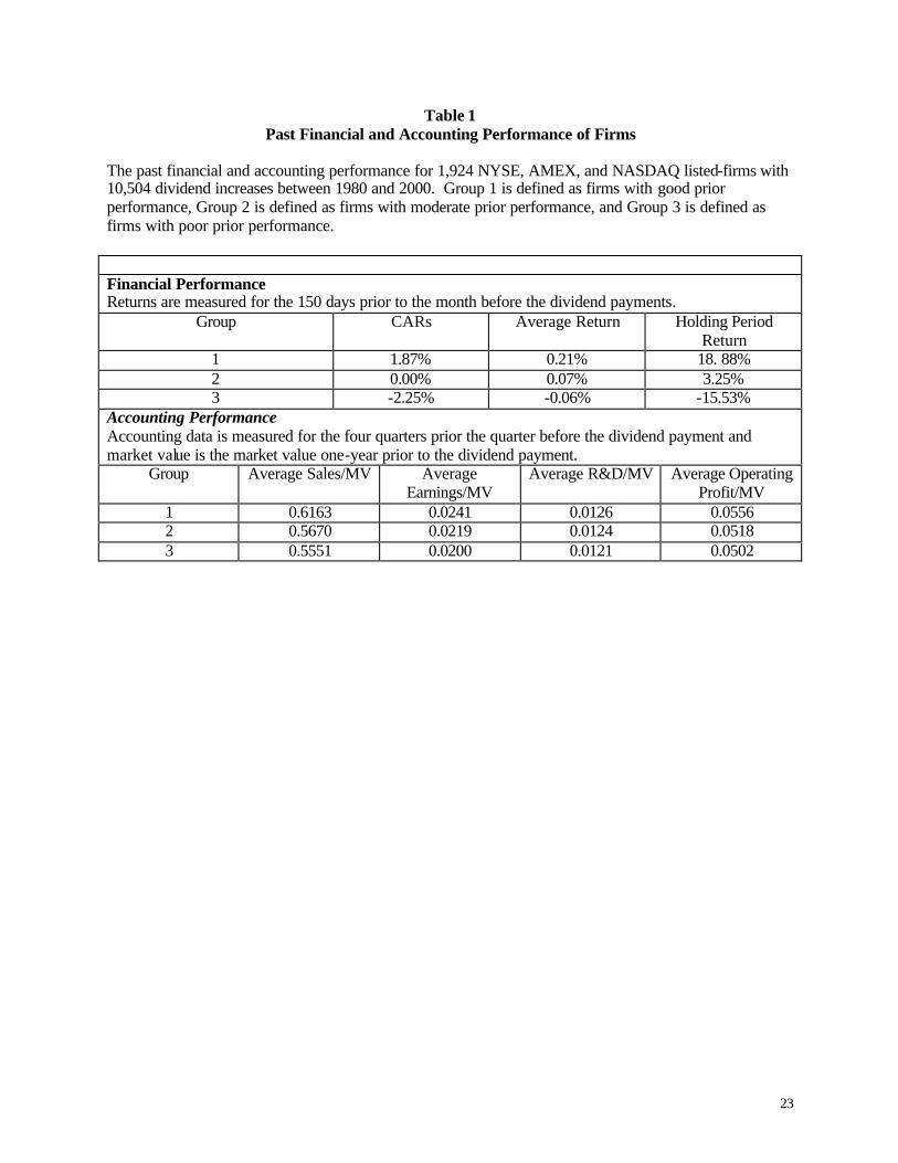
As a robustness check of our prior-financial-performance partition, for each firm we also

collected accounting measures of performance for one year prior to the quarter in which the dividend

increase was announced. These measures were scaled by the market value of the firm measured at the

beginning of the year for which the accounting data were collected. As Table 1 indicates, the average

returns, average sales-to-market-value, average earnings-to-market-value, average R&D-to-market-value

(when available), and average operating profit-to-market-value are all monotonically increasing in the

firm quality for all three groups, with the good-prior-performance group having the best prior

performance and the poor-prior-performance group having the worst.

Table 1 goes here

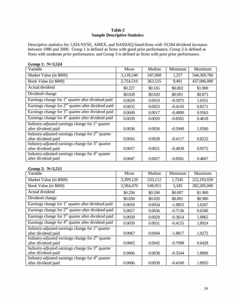
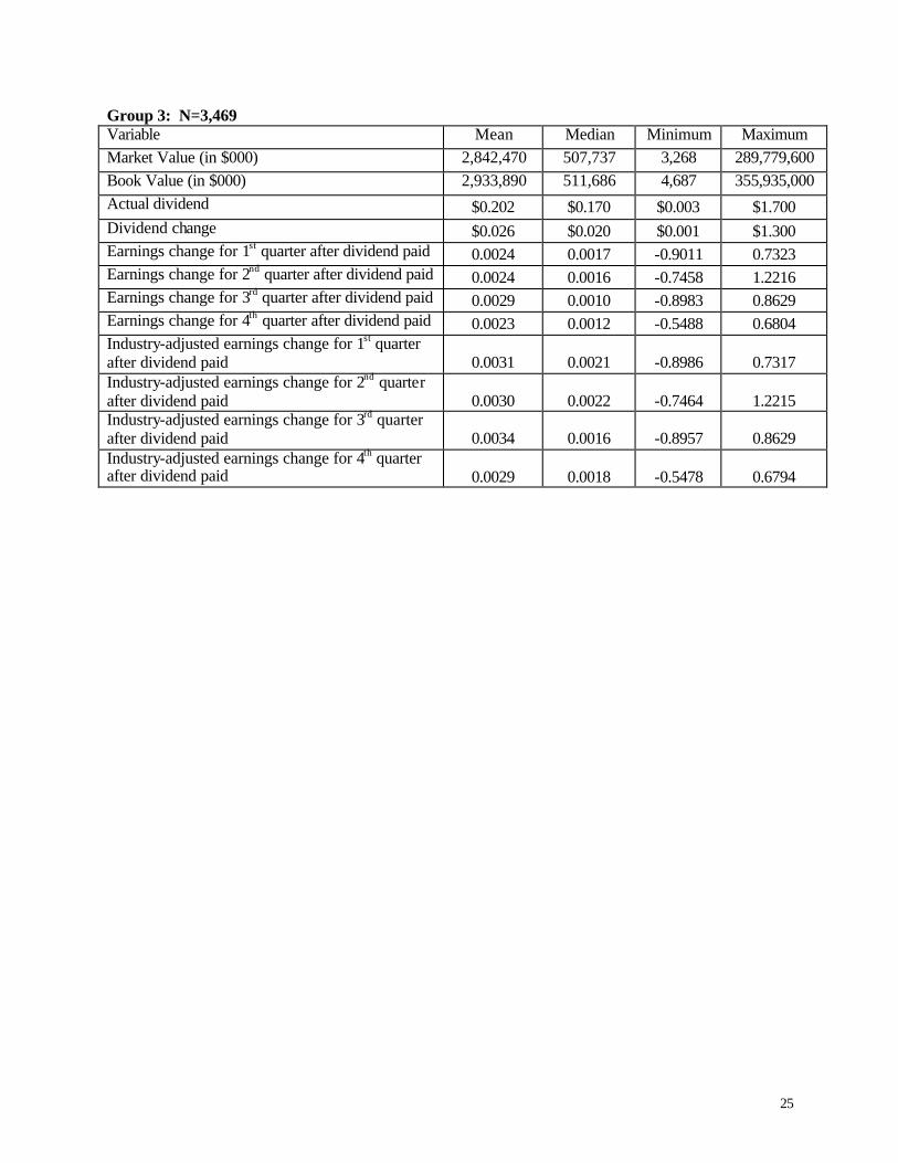
Table 2 reports the descriptive statistics for our sample of firms.

Table 2 goes here

C. The Tests and Results

We begin by testing Hypothesis A that firms with poor prior performance pay the lowest

dividends and have less intragroup heterogeneity in future earnings than do firms with moderate prior

performance. We investigate the dividend payments first. As indicated in Table 3 Panel A, the poor-

performance group has an average dividend payment of $0.202 and an average dividend increase of

$0.026, the moderate-performance group has an average dividend payment of $0.256 and an average

dividend increase of $0.030, and the good-performance group has an average dividend payment of $0.223

and an average dividend increase of $0.028. The difference-of-means tests for the actual dividends paid

and the dividend increases are significant at the one-percent or five-percent level. Thus, firms with poor

prior performance pay the lowest dividends of all groups and have the lowest dividend increases.

7 For each of the three measures of prior performance (CARs, average returns, BHARs), the following empirical results are qualitatively similar. We present here the results based on partitioning by CARs; the results using

15

Table 3 goes here

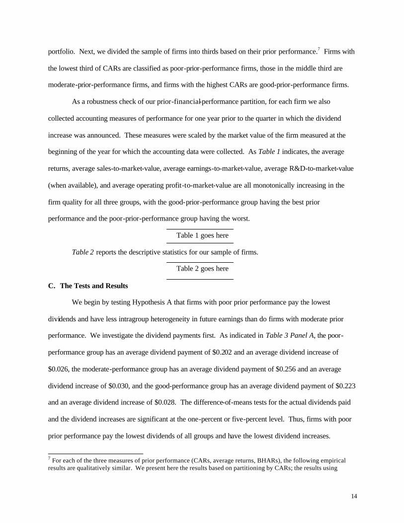
Next, we examine if the intragroup variation in future earnings is larger for the moderate -

performance firms than for the poor-performance firms. We use two methods to estimate unexpected

future earnings. The first estimate is Benartzi, Michaely, and Thaler's (1997) estimate of future earnings

that assumes earnings follow a random walk with a drift; earnings this quarter should equal earnings last

quarter plus the average growth rate from quarters –5 to –1. Therefore, unexpected future earnings are

i,t i,t 1 i,t 1 i,t 5i,t

i,t 1

( E E ) ( E E ) / 4UE ,

MV− − −

−

− − −= (1)

where UEi,t is the unexpected earnings of firm i in quarter t, Ei,t is its earnings in quarter t, and MVi,t -1 is

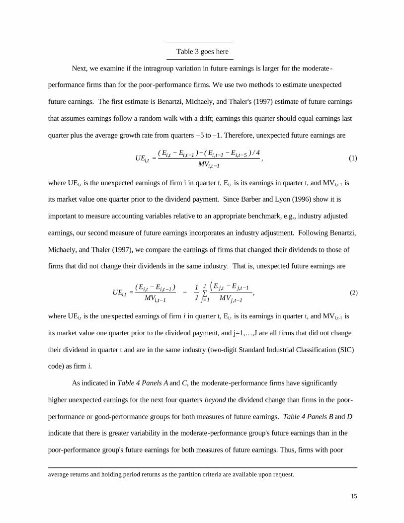
its market value one quarter prior to the dividend payment. Since Barber and Lyon (1996) show it is

important to measure accounting variables relative to an appropriate benchmark, e.g., industry adjusted

earnings, our second measure of future earnings incorporates an industry adjustment. Following Benartzi,

Michaely, and Thaler (1997), we compare the earnings of firms that changed their dividends to those of

firms that did not change their dividends in the same industry. That is, unexpected future earnings are

( )J j,t j,t 1i,t i,t 1i,t

j 1i,t 1 j,t 1

E E( E E ) 1UE ,

MV J MV−−

=− −

−−= − ∑ (2)

where UEi,t is the unexpected earnings of firm i in quarter t, Ei,t is its earnings in quarter t, and MVi,t -1 is

its market value one quarter prior to the dividend payment, and j=1,…,J are all firms that did not change

their dividend in quarter t and are in the same industry (two-digit Standard Industrial Classification (SIC)

code) as firm i.

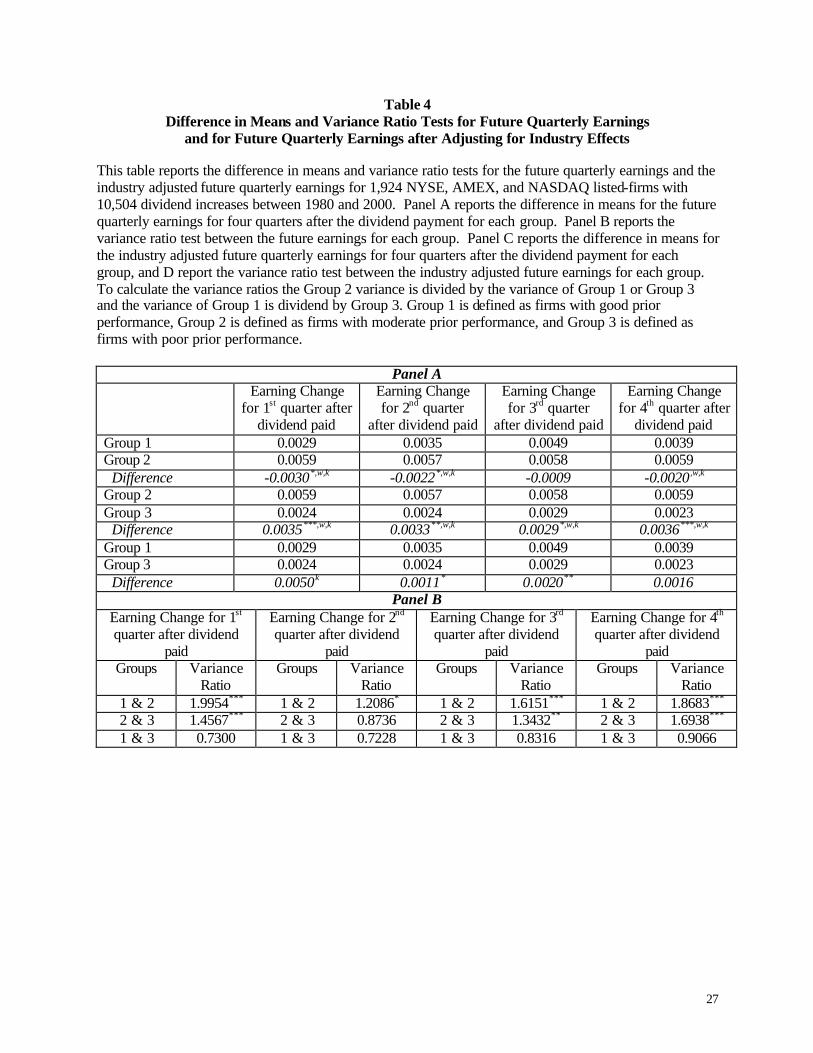
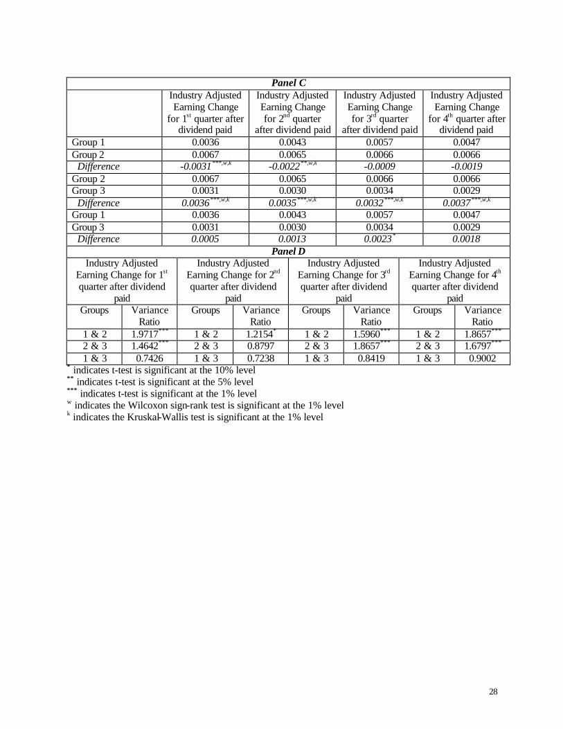
As indicated in Table 4 Panels A and C, the moderate-performance firms have significantly

higher unexpected earnings for the next four quarters beyond the dividend change than firms in the poor-

performance or good-performance groups for both measures of future earnings. Table 4 Panels B and D

indicate that there is greater variability in the moderate-performance group's future earnings than in the

poor-performance group's future earnings for both measures of future earnings. Thus, firms with poor

average returns and holding period returns as the partition criteria are available upon request.

16

prior performance have significantly less heterogeneity in their future earnings than do moderate-prior-

performance firms.

Table 4 goes here

We then turn to Hypothesis B, which says that firms that have had good prior performance will

have less heterogeneity in future earnings than firms with moderate prior performance. As reported in

Table 4 Panels B and D, good-prior-performance firms have less variability in future earnings than

moderate-prior-performance firms for four quarters after the dividend increase. Further, Table 4 Panels A

and C show that the moderate-performance firms have significantly larger future earnings than the good-

performance firms but only for two quarters after the dividend increase.

Next, we test Hypothesis C that firms with moderate prior performance have the largest

intragroup heterogeneity in current dividend payments and in past and future earnings when compared to

firms with good or poor prior performance. Table 3 Panel B indicates that firms with moderate prior

performance have the largest intragroup variation in current dividend payments compared to the other

groups. However, all groups have similar intragroup variations in their dividend increases. Table 4

Panels B and C also show that moderate-prior-performance firms have significantly higher intragroup

variability in future earnings, for both measure of unexpected future earnings, than firms with either poor

or good prior performance.

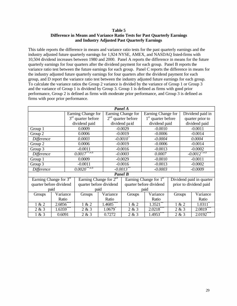
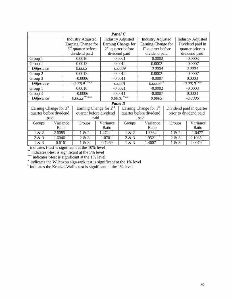
Next, we test to see if the past earnings of groups with moderate prior performance exhibit higher

intragroup variance than the past earnings of firms with good or poor prior performance. Again we

measure unexpected past earnings for four quarters prior to the dividend announcement using equations

(1) and (2). Table 5 Panels A and C shows that the past earnings for firms in all three groups, while Table

5 Panels B and D report the variance ratio tests for the past earnings. Firms with moderate prior

performance display significantly higher intragroup variance in past earnings, regardless of how earnings

are measured, than do firms with either poor or good prior performance.

Table 5 goes here

17

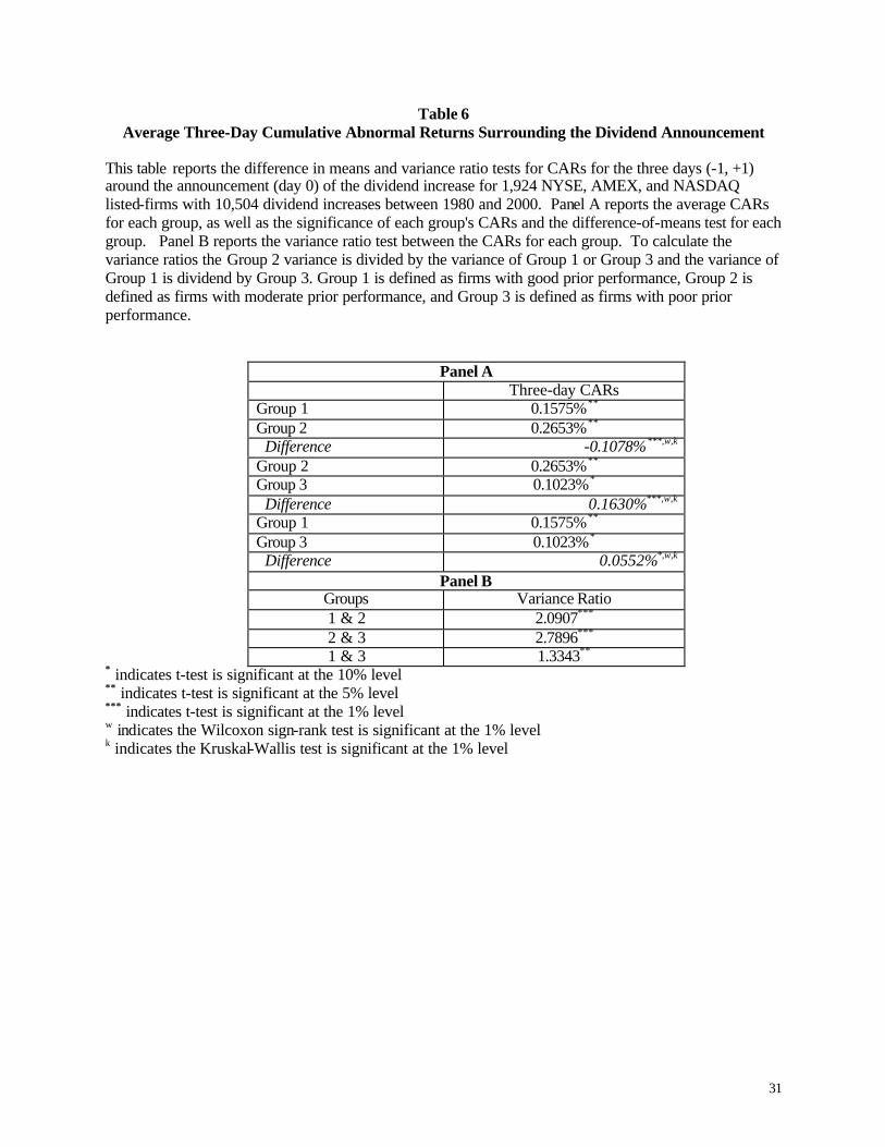
Hypothesis D is tested to determine if the CARs for the three days (t=-1,+1) around the

announcement day (t=0) of the dividend increase are the highest for the firms in the moderate prior

performance group. As indicated in Table 6 Panel A, firms with moderate prior performance have

significantly higher CARs than firms with good or poor prior performance.

Table 6 goes here

Finally, we test Hypothesis E to determine if the CARs for firms with moderate prior

performance have greater intragroup heterogeneity than the CARs of firms with poor or good prior

performance firms, and if the average dividend payment or dividend increase is the highest for firms with

moderate prior performance. Table 6 Panel B reports that the intragroup variability in the CARs for firms

with moderate prior performance is significantly greater than that of firms with poor or good prior

performance. Table 3 Panel A shows that firms with moderate prior performance pay significantly higher

dividends than firms with good and poor prior performance. Further, firms with moderate prior

performance also have significantly larger average dividend increase than those for firms with poor and

good prior performance.

So far, all our tests have been univariate. However, we would like to control for other factors that

impact CARs and dividend payments, most notably firm size, growth opportunities and dividend yield.

The purpose of doing this is to examine whether our findings are attributable to factors outside our model.

First, we test the prediction that firms with mediocre prior performance will have the largest

dividend payment, firms with good prior performance will have the next largest dividend change, and

firms with poor prior performance will have the smallest dividend change. We create three dummy

variables that classify the firms based on their prior performance: poor, mediocre, or good. We proxy for

growth opportunities using the market-to-book ratio for the firm calculated the month prior to the

dividend announcement, and the dividend yield is the prior yearly dividend payment divided by the

closing price of that year. We estimate the following regression equation:

Poor Mediocre Good Lsize Mktbk DivYld= β + β + β + β + β + β + ε1 2 3 4 5 6∆ (3)

18

where ∆ is the actual dividend payment or the dividend increase standardized by the firm's price one

week prior to the announcement, Poor is 1 if the firm has poor prior performance and 0 otherwise,

Mediocre is 1 if the firm has mediocre prior performance and 0 otherwise, Good is 1 if the firm has good

prior performance and 0 otherwise, Lsize is the log of the market capitalization of the firm as of one

month prior to the dividend announcement, Mktbk is the firm's market-to-book ratio one month prior to

the dividend announcement, DivYld is the firm’s dividend yield for the year prior to the dividend

announcement, and , is the ordinary least squares error.

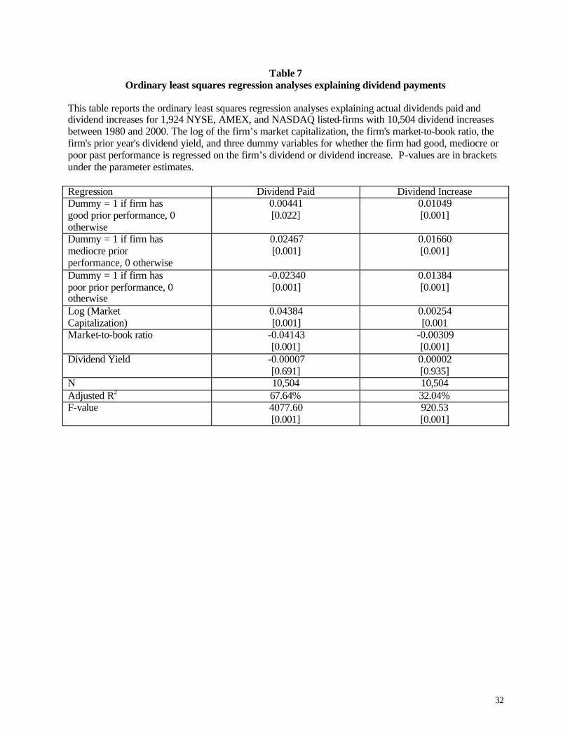
Table 7 indicates the regression results when ∆ is the actual dividend paid and when ∆ equals

the dividend increase. For both regressions the coefficients on Poor, Mediocre and Good follow the

nonmonotonic relation predicted by the theoretical argument even when controlling for size, growth

opportunities, and dividend yield. Further, the F-test indicates that the coefficients for Poor, Mediocre,

and Good are significantly different from each other at the one-percent level (F-value=46.42 for the actual

dividend paid and F-value=19.69 for the dividend increase). Further, we test if the coefficients for Poor

and Mediocre, Mediocre and Good, and Poor and Good are significantly different from each other and

find that all pairs are significantly different from each other for both regressions at the one-percent level.

Firm size has a significant and positive impact on the dividend paid and the dividend increase, whereas

growth opportunities have a negative and significant impact on the dividend paid and the dividend

increase. These results can be understood within the context of Fama and French (2001). Fama and

French find that large firms and firms with few growth opportunities generally pay more in dividends.

Thus, we would expect a positive relation between firm size and the dividend paid and the dividend

increase and a negative relation between the firm's growth opportunities and the dividend paid and the

dividend increase. The firm’s dividend yield does not have a significant impact on the actual dividend

paid or the dividend increase.

Table 7 goes here

19

Next, we test the prediction that firms with mediocre prior performance will have larger

announcement-day CARs than firms with good and poor prior performance. We estimate the following

regression equation:

CARs Poor Mediocre Good Lsize Mktbk DivYld= β + β + β + β + β + β + ε1 2 3 4 5 6 (4)

where CARs is the CARs for three days (t=-1,+1) around the announcement day of the dividend increase

and all other variables are as defined for equation (3).

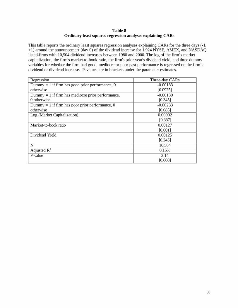
Table 8 indicates that firms with mediocre prior performance have the highest CARs while firm

with good prior performance have the next highest CARs and firms with poor prior performance have the

lowest CARs. However, the F-test of whether the coefficients for Poor, Mediocre, and Good are

significantly different from each other is not significant, nor are the tests of paired significance. As with

all regressions that attempt to explain abnormal returns, because of the low explanatory power of the

regression, the results must be viewed with skepticism, although the F-statistic for the equation is positive

and significant. Further, firm size and divided yield are both insignificant determents of CARs. The

market-to-book ratio has a positive and significant relation with CARs. Thus, the larger the growth

opportunity, the larger the price reaction to a dividend increase.

Table 8 goes here

V. CONCLUSION

We have developed an argument in which firms pay dividends to signal future cash flow and/or to

disburse excess cash flows. Since firms can be classified into three observationally distinct groups using

their prior performance, signaling occurs only within each group and not across groups. Thus, if one

lumps all these firms together in examining their dividend payments and the stock price reactions to them,

one can encounter all sorts of nonmonotonicities. Our argument captures the notions of heterogeneity

across a priori observationally distinct groups and heterogeneity within a group of observationally

identical firms. We hypothesize that firms with the poorest prior performance pay the lowest dividends

because they are (correctly) identified by their prior performance and thus have nothing to signal;

20

moreover, they face a relatively small FCF problem. The firms with the best prior performance are

(correctly) identified as such, so they have no signaling concerns and pay somewhat higher dividends to

cope with their larger FCF problem. However, firms with intermediate prior performance pay dividends

to solve their FCF problem and also to signal in order to separate themselves from each other. Thus, the

intermediate-type firms, which should have the highest intragroup heterogeneity in past and future

earnings as well as dividends and price announcement effects, may pay larger dividends than the highest-

type firms and the lowest-type firms. This integration of the signaling and FCF hypotheses allows us to

develop a new way to examine the data.

The empirical tests support our predictions. In particular, there is a nonmonotonic relationship

between firm "quality" and dividends. Moreover, we find that firms that have had poor or good prior

performance will display very little heterogeneity in future earnings, while firms with moderate prior

performance will have high future and past earnings heterogeneity and have the highest heterogeneity in

current dividend payments. Finally, we find that firms with moderate prior performance will have the

highest abnormal price reaction to a dividend change.

Our empirical finding that dividends are nonmonotonic in observed firm quality is important

because it validates our motivating intuition that the weakness of the empirical support for the dividend-

signaling hypothesis may be due to this nonmonotonicity. Because of the potential confounding between

what the market knows and what it does not know at the time of signaling that is likely to be encountered

in many signaling situations, we believe that the FCF-cum-signaling argument developed here may be

useful in many other contexts as well. Capital structure signaling comes first to mind, but there may be

others too.

21

References Allen, F., and R. Michaely, 2002, “Payout Policy,” working paper, April, forthcoming in North-Holland

Handbook of Economics (eds. G. Constantinides, M. Harris and R. Stulz). Barber, B., and J. Lyon, 1996, “Detecting Abnormal Operating Performance: The Empirical Power

and Specification of Test Statistics,” Journal of Financial Economics 41, 359-399. Barber, B., and J. Lyon, 1997, “Detecting Long-Run Abnormal Stock Returns: The Empirical Power and

Specification of Test Statistics,” Journal of Financial Economics 43, 341-372. Benartzi, S., R. Michaely, and R. Thaler, 1997, “Do Changes in Dividends Signal the Future or the Past?”

Journal of Finance 52, 1007-1034. Bhattacharya, S., 1979, “Imperfect Information, Dividend Policy, and ‘The Bird in the Hand’ Fallacy,”

Bell Journal of Economics 10, 259-270. Brown, S., and Warner, J., 1980, “Measuring Security Price Performance,” Journal of Financial

Economics 8, 205-258. Brown, S., and Warner, J., 1985, “Using Daily Stock Returns,” Journal of Financial Economics 14, 3-31. Easterbrook, F., 1984, “Two Agency-cost Explanations of Dividends,” American Economic Review 74,

650-659. Fama, E., 1998, “Market Efficiency, Long-Term Returns, and Behavioral Finance,” Journal of Financial

Economics 49, 283-306. Fama, E., and K. French, 2001, “Disappearing Dividends: Changing Firm Characteristics or Lower

Propensity to Pay?,” Journal of Financial Economics 60, 3-43. Grullon, G., R. Michaely, B. Swaminathan, 2002, “Are Dividend Changes a Sign of Firm Maturity?”

Journal of Business, forthcoming. Jensen, M., 1986, “Agency Costs of Free Cash Flow, Corporate Finance, and Takeovers,” American

Economic Review 76, 323-329. John, K., and J. Williams, 1985, “Dividends, Dilution, and Taxes: a Signaling Equilibrium,” Journal of

Finance 40, 1053-1070. Lang, L., and R. Litzenberger, 1989, “Dividend Announcements: Cash Flow Signaling vs. Free Cash

Flow Hypothesis?,” Journal of Financial Economics 24, 181-192. Lie, E., 2000, “Excess Funds and Agency Problems: An Empirical Study of Incremental Cash

Disbursements,” Review of Financial Studies 13, 219-248. Miller, M., and K. Rock, 1985, “Dividend Policy under Asymmetric Information,” Journal of Finance 40,

1031-1051. Miller, M., and F. Modigliani, 1961, “Dividend Policy, Growth and the Valuation of Shares,” Journal of

22

Business 34, 411-433. Ofer, A., and A.V. Thakor, 1987, “A Theory of Stock Price Responses to Alternative Corporate Cash Disbursement Methods: Stock Repurchases and Dividends,” Journal of Finance 42, 365-394. Yoon, P., and L. Starks, 1995, “Signaling, Investment Opportunities, and Dividend Announcements,”

Review of Financial Studies 8, 995-1018.

23

Table 1 Past Financial and Accounting Performance of Firms

The past financial and accounting performance for 1,924 NYSE, AMEX, and NASDAQ listed-firms with 10,504 dividend increases between 1980 and 2000. Group 1 is defined as firms with good prior performance, Group 2 is defined as firms with moderate prior performance, and Group 3 is defined as firms with poor prior performance.

Financial Performance Returns are measured for the 150 days prior to the month before the dividend payments.

Group CARs Average Return Holding Period Return

1 1.87% 0.21% 18. 88% 2 0.00% 0.07% 3.25% 3 -2.25% -0.06% -15.53%

Accounting Performance Accounting data is measured for the four quarters prior the quarter before the dividend payment and market value is the market value one-year prior to the dividend payment.

Group Average Sales/MV Average Earnings/MV

Average R&D/MV Average Operating Profit/MV

1 0.6163 0.0241 0.0126 0.0556 2 0.5670 0.0219 0.0124 0.0518 3 0.5551 0.0200 0.0121 0.0502

24

Table 2 Sample Descriptive Statistics

Descriptive statistics for 1,924 NYSE, AMEX, and NASDAQ listed-firms with 10,504 dividend increases between 1980 and 2000. Group 1 is defined as firms with good prior performance, Group 2 is defined as firms with moderate prior performance, and Group 3 is defined as firms with poor prior performance. Group 1: N=3,524 Variable Mean Median Minimum Maximum Market Value (in $000) 3,139,240 347,068 1,257 544,369,760 Book Value (in $000) 2,754,510 363,525 9,491 437,006,000 Actual dividend $0.227 $0.165 $0.002 $1.900 Dividend change $0.028 $0.020 $0.001 $0.873 Earnings change for 1st quarter after dividend paid 0.0029 0.0019 -0.5975 1.0551 Earnings change for 2nd quarter after dividend paid 0.0035 0.0023 -0.4143 0.8171 Earnings change for 3rd quarter after dividend paid 0.0049 0.0017 -0.4890 0.9563 Earnings change for 4th quarter after dividend paid 0.0039 0.0020 -0.8581 0.4618 Industry-adjusted earnings change for 1st quarter after dividend paid 0.0036 0.0026 -0.5949 1.0560 Industry-adjusted earnings change for 2nd quarter after dividend paid 0.0043 0.0028 -0.4117 0.8222 Industry-adjusted earnings change for 3rd quarter after dividend paid 0.0057 0.0021 -0.4839 0.9572 Industry-adjusted earnings change for 4th quarter after dividend paid 0.0047 0.0027 -0.8581 0.4607 Group 2: N=3,511 Variable Mean Median Minimum Maximum Market Value (in $000) 3,399,120 533,112 1,7545 252,193,030 Book Value (in $000) 3,584,470 548,951 5,345 282,285,000 Actual dividend $0.256 $0.200 $0.007 $1.900 Dividend change $0.030 $0.020 $0.001 $0.980 Earnings change for 1st quarter after dividend paid 0.0059 0.0034 -1.8855 1.0267 Earnings change for 2nd quarter after dividend paid 0.0057 0.0036 -0.7136 0.6396 Earnings change for 3rd quarter after dividend paid 0.0058 0.0029 -0.3614 1.8865 Earnings change for 4th quarter after dividend paid 0.0059 0.0031 -0.4155 1.8924 Industry-adjusted earnings change for 1st quarter after dividend paid 0.0067 0.0044 -1.8817 1.0272 Industry-adjusted earnings change for 2nd quarter after dividend paid 0.0065 0.0042 -0.7098 0.6428 Industry-adjusted earnings change for 3rd quarter after dividend paid 0.0066 0.0038 -0.3544 1.8896 Industry-adjusted earnings change for 4th quarter after dividend paid 0.0066 0.0039 -0.4160 1.8955

25

Group 3: N=3,469 Variable Mean Median Minimum Maximum Market Value (in $000) 2,842,470 507,737 3,268 289,779,600 Book Value (in $000) 2,933,890 511,686 4,687 355,935,000 Actual dividend $0.202 $0.170 $0.003 $1.700 Dividend change $0.026 $0.020 $0.001 $1.300 Earnings change for 1st quarter after dividend paid 0.0024 0.0017 -0.9011 0.7323 Earnings change for 2nd quarter after dividend paid 0.0024 0.0016 -0.7458 1.2216 Earnings change for 3rd quarter after dividend paid 0.0029 0.0010 -0.8983 0.8629 Earnings change for 4th quarter after dividend paid 0.0023 0.0012 -0.5488 0.6804 Industry-adjusted earnings change for 1st quarter after dividend paid 0.0031 0.0021 -0.8986 0.7317 Industry-adjusted earnings change for 2nd quarter after dividend paid 0.0030 0.0022 -0.7464 1.2215 Industry-adjusted earnings change for 3rd quarter after dividend paid 0.0034 0.0016 -0.8957 0.8629 Industry-adjusted earnings change for 4th quarter after dividend paid 0.0029 0.0018 -0.5478 0.6794

26

Table 3 Difference in Means and Variance Ratio Tests for Actual Dividend Paid

and the Dividend Change

Panel A reports the difference in means for the actual dividend paid and the dividend change for 1,924 NYSE, AMEX, and NASDAQ listed-firms with 10,504 dividend increases between 1980 and 2000. Panel B shows the variance ratio tests for the actual dividend paid and the unexpected dividend change. To calculate the variance ratios the Group 2 variance is divided by the variance of Group 1 or Group 3 and the variance of Group 1 is dividend by Group 3. Group 1 is defined as firms with good prior performance, Group 2 is defined as firms with moderate prior performance, and Group 3 is defined as firms with poor prior performance.

Panel A Dividend paid Dividend increase

Group 1 $0.223 $0.028 Group 2 $0.256 $0.030 Difference $-0.039***,w,k $-0.002**,w,k

Group 2 $0.256 $0.030 Group 3 $0.223 $0.026 Difference $0.033***,w,k $0.004***,w,k

Group 1 $0.223 $0.028 Group 3 $0.202 $0.026 Difference $0.021**,w,k $0.002**,w,k

Panel B Dividend paid Dividend increase

Groups Variance Ratio Groups Variance Ratio 1 & 2 1.4513*** 1 & 2 0.8844 2 & 3 1.3325** 2 & 3 0.7836 1 & 3 0.9181 1 & 3 0.8860

* indicates t-test is significant at the 10% level ** indicates t-test is significant at the 5% level *** indicates t-test is significant at the 1% level w indicates the Wilcoxon sign-rank test is significant at the 1% level k indicates the Kruskal-Wallis test is significant at the 1% level

27

Table 4 Difference in Means and Variance Ratio Tests for Future Quarterly Earnings

and for Future Quarterly Earnings after Adjusting for Industry Effects

This table reports the difference in means and variance ratio tests for the future quarterly earnings and the industry adjusted future quarterly earnings for 1,924 NYSE, AMEX, and NASDAQ listed-firms with 10,504 dividend increases between 1980 and 2000. Panel A reports the difference in means for the future quarterly earnings for four quarters after the dividend payment for each group. Panel B reports the variance ratio test between the future earnings for each group. Panel C reports the difference in means for the industry adjusted future quarterly earnings for four quarters after the dividend payment for each group, and D report the variance ratio test between the industry adjusted future earnings for each group. To calculate the variance ratios the Group 2 variance is divided by the variance of Group 1 or Group 3 and the variance of Group 1 is dividend by Group 3. Group 1 is defined as firms with good prior performance, Group 2 is defined as firms with moderate prior performance, and Group 3 is defined as firms with poor prior performance.

Panel A Earning Change

for 1st quarter after dividend paid

Earning Change for 2nd quarter

after dividend paid

Earning Change for 3rd quarter

after dividend paid

Earning Change for 4th quarter after

dividend paid Group 1 0.0029 0.0035 0.0049 0.0039 Group 2 0.0059 0.0057 0.0058 0.0059 Difference -0.0030*,w,k -0.0022*,w,k -0.0009 -0.0020 ,w,k Group 2 0.0059 0.0057 0.0058 0.0059 Group 3 0.0024 0.0024 0.0029 0.0023 Difference 0.0035***,w,k 0.0033**,w,k 0.0029*,w,k 0.0036***,w,k Group 1 0.0029 0.0035 0.0049 0.0039 Group 3 0.0024 0.0024 0.0029 0.0023 Difference 0.0050k 0.0011* 0.0020** 0.0016

Panel B Earning Change for 1st quarter after dividend

paid

Earning Change for 2nd quarter after dividend

paid

Earning Change for 3rd quarter after dividend

paid

Earning Change for 4th quarter after dividend

paid Groups Variance

Ratio Groups Variance



Ratio 1 & 2 1.9954*** 1 & 2 1.2086* 1 & 2 1.6151*** 1 & 2 1.8683*** 2 & 3 1.4567*** 2 & 3 0.8736 2 & 3 1.3432** 2 & 3 1.6938*** 1 & 3 0.7300 1 & 3 0.7228 1 & 3 0.8316 1 & 3 0.9066

28

Panel C

Industry Adjusted Earning Change

for 1st quarter after dividend paid

Industry Adjusted Earning Change for 2nd quarter

after dividend paid

Industry Adjusted Earning Change for 3rd quarter

after dividend paid

Industry Adjusted Earning Change

for 4th quarter after dividend paid

Group 1 0.0036 0.0043 0.0057 0.0047 Group 2 0.0067 0.0065 0.0066 0.0066 Difference -0.0031***,w,k -0.0022**,w,k -0.0009 -0.0019 Group 2 0.0067 0.0065 0.0066 0.0066 Group 3 0.0031 0.0030 0.0034 0.0029 Difference 0.0036***,w,k 0.0035***,w,k 0.0032***,w,k 0.0037***,w,k Group 1 0.0036 0.0043 0.0057 0.0047 Group 3 0.0031 0.0030 0.0034 0.0029 Difference 0.0005 0.0013 0.0023* 0.0018

Panel D Industry Adjusted

Earning Change for 1st quarter after dividend

paid

Industry Adjusted Earning Change for 2nd quarter after dividend

paid

Industry Adjusted Earning Change for 3rd quarter after dividend

paid

Industry Adjusted Earning Change for 4th quarter after dividend

paid Groups Variance




Ratio 1 & 2 1.9717*** 1 & 2 1.2154* 1 & 2 1.5960*** 1 & 2 1.8657*** 2 & 3 1.4642*** 2 & 3 0.8797 2 & 3 1.8657*** 2 & 3 1.6797*** 1 & 3 0.7426 1 & 3 0.7238 1 & 3 0.8419 1 & 3 0.9002


29

Table 5 Difference in Means and Variance Ratio Tests for Past Quarterly Earnings

and Industry Adjusted Past Quarterly Earnings

This table reports the difference in means and variance ratio tests for the past quarterly earnings and the industry adjusted future quarterly earnings for 1,924 NYSE, AMEX, and NASDAQ listed-firms with 10,504 dividend increases between 1980 and 2000. Panel A reports the difference in means for the future quarterly earnings for four quarters after the dividend payment for each group. Panel B reports the variance ratio test between the future earnings for each group. Panel C reports the difference in means for the industry adjusted future quarterly earnings for four quarters after the dividend payment for each group, and D report the variance ratio test between the industry adjusted future earnings for each group. To calculate the variance ratios the Group 2 variance is divided by the variance of Group 1 or Group 3 and the variance of Group 1 is dividend by Group 3. Group 1 is defined as firms with good prior performance, Group 2 is defined as firms with moderate prior performance, and Group 3 is defined as firms with poor prior performance.

Panel A Earning Change for

3rd quarter before dividend paid

Earning Change for 2nd quarter before

dividend pa id

Earning Change for 1st quarter before

dividend paid

Dividend paid in quarter prior to dividend paid

Group 1 0.0009 -0.0029 -0.0010 -0.0011 Group 2 0.0006 -0.0019 -0.0006 -0.0014 Difference 0.0003 -0.0010* -0.0004 0.0004 Group 2 0.0006 -0.0019 -0.0006 -0.0014 Group 3 -0.0011 -0.0016 -0.0013 -0.0002 Difference 0.0017**,w,k -0.0003 0.0007 -0.0012*,w,k Group 1 0.0009 -0.0029 -0.0010 -0.0011 Group 3 -0.0011 -0.0016 -0.0013 -0.0002 Difference 0.0020**,w,k -0.0013** -0.0003 -0.0009

Panel B Earning Change for 3rd quarter before dividend

paid

Earning Change for 2nd quarter before dividend

paid

Earning Change for 1st quarter before dividend

paid


Groups Variance Ratio




1 & 2 2.6856*** 1 & 2 1.4685*** 1 & 2 1.3521** 1 & 2 1.0311* 2 & 3 1.6359*** 2 & 3 1.0679* 2 & 3 2.0218*** 2 & 3 2.0819*** 1 & 3 0.6091 2 & 3 0.7272 2 & 3 1.4953*** 2 & 3 2.0192***

30

Panel C

Industry Adjusted Earning Change for 3rd quarter before

dividend paid

Industry Adjusted Earning Change for 2nd quarter before

dividend paid

Industry Adjusted Earning Change for 1st quarter before

dividend paid

Industry Adjusted Dividend paid in quarter prior to dividend paid

Group 1 0.0016 -0.0021 -0.0002 -0.0003 Group 2 0.0013 -0.0012 0.0002 -0.0007 Difference 0.0003 -0.0009 -0.0004 0.0004 Group 2 0.0013 -0.0012 0.0002 -0.0007 Group 3 -0.0006 -0.0011 -0.0007 0.0003 Difference -0.0019**,w,k -0.0001 0.0009w,k -0.0010*,w,k Group 1 0.0016 -0.0021 -0.0002 -0.0003 Group 3 -0.0006 -0.0011 -0.0007 0.0003 Difference 0.0022***,w,k 0.0010*,w,k 0.0005 -0.0006

Panel D Earning Change for 3rd quarter before dividend

paid

Earning Change for 2nd quarter before dividend

paid

Earning Change for 1st quarter before dividend

paid






1 & 2 2.6085*** 1 & 2 1.4722*** 1 & 2 1.3364** 1 & 2 1.0477* 2 & 3 1.6046*** 2 & 3 1.0701* 2 & 3 1.9521*** 2 & 3 2.1035*** 1 & 3 0.6161 1 & 3 0.7269 1 & 3 1.4607*** 1 & 3 2.0079***


31

Table 6 Average Three-Day Cumulative Abnormal Returns Surrounding the Dividend Announcement

This table reports the difference in means and variance ratio tests for CARs for the three days (-1, +1) around the announcement (day 0) of the dividend increase for 1,924 NYSE, AMEX, and NASDAQ listed-firms with 10,504 dividend increases between 1980 and 2000. Panel A reports the average CARs for each group, as well as the significance of each group's CARs and the difference-of-means test for each group. Panel B reports the variance ratio test between the CARs for each group. To calculate the variance ratios the Group 2 variance is divided by the variance of Group 1 or Group 3 and the variance of Group 1 is dividend by Group 3. Group 1 is defined as firms with good prior performance, Group 2 is defined as firms with moderate prior performance, and Group 3 is defined as firms with poor prior performance.

Panel A Three-day CARs

Group 1 0.1575%** Group 2 0.2653%** Difference -0.1078%***,w,k Group 2 0.2653%** Group 3 0.1023%* Difference 0.1630%***,w,k Group 1 0.1575%** Group 3 0.1023%* Difference 0.0552%*,w,k

Panel B Groups Variance Ratio 1 & 2 2.0907***

2 & 3 2.7896***

1 & 3 1.3343**


32

Table 7 Ordinary least squares regression analyses explaining dividend payments

This table reports the ordinary least squares regression analyses explaining actual dividends paid and dividend increases for 1,924 NYSE, AMEX, and NASDAQ listed-firms with 10,504 dividend increases between 1980 and 2000. The log of the firm’s market capitalization, the firm's market-to-book ratio, the firm's prior year's dividend yield, and three dummy variables for whether the firm had good, mediocre or poor past performance is regressed on the firm’s dividend or dividend increase. P-values are in brackets under the parameter estimates. Regression Dividend Paid Dividend Increase Dummy = 1 if firm has good prior performance, 0 otherwise

0.00441 [0.022]

0.01049 [0.001]

Dummy = 1 if firm has mediocre prior performance, 0 otherwise

0.02467 [0.001]

0.01660 [0.001]

Dummy = 1 if firm has poor prior performance, 0 otherwise

-0.02340 [0.001]

0.01384 [0.001]

Log (Market Capitalization)

0.04384 [0.001]

0.00254 [0.001

Market-to-book ratio -0.04143 [0.001]

-0.00309 [0.001]

Dividend Yield -0.00007 [0.691]

0.00002 [0.935]

N 10,504 10,504 Adjusted R2 67.64% 32.04% F-value 4077.60

[0.001] 920.53 [0.001]

33

Table 8 Ordinary least squares regression analyses explaining CARs

This table reports the ordinary least squares regression analyses explaining CARs for the three days (-1, +1) around the announcement (day 0) of the dividend increase for 1,924 NYSE, AMEX, and NASDAQ listed-firms with 10,504 dividend increases between 1980 and 2000. The log of the firm’s market capitalization, the firm's market-to-book ratio, the firm's prior year's dividend yield, and three dummy variables for whether the firm had good, mediocre or poor past performance is regressed on the firm’s dividend or dividend increase. P-values are in brackets under the parameter estimates. Regression Three-day CARs Dummy = 1 if firm has good prior performance, 0 otherwise

-0.00183 [0.0925]

Dummy = 1 if firm has mediocre prior performance, 0 otherwise

-0.00130 [0.345]

Dummy = 1 if firm has poor prior performance, 0 otherwise

-0.00233 [0.085]

Log (Market Capitalization) 0.00002 [0.887]

Market-to-book ratio 0.00127 [0.001]

Dividend Yield 0.00125 [0.245]

N 10,504 Adjusted R2 0.15% F-value 3.14

[0.008]

34

Figure 1 Time Line

t = 0 t = 2 t = 1

• Two types of firms exist, good and bad quality.

• Past performance of each firm is observed.

• Market receives signal, s ∈{0, L, H}, that conveys information about cash flows at t=2.

• Based on the signal s, firms now fall into three observationally distinct groups.

• All firms look identical to the market.

• Firms realize cash flows of H, L or 0.

• Dividend, d, is

paid. • Managers waste

excess cash flow, if available

• Firms announce dividend, d, paid at t=2.

35

Figure 2 Dividends and Firm Quality

Dividends

Firm quality

3Bd

1Gd

2d

Poor prior performance (group 3) firms

Moderate prior performance (group 2) firms

Good prior performance (group 1) firms

signaling, free cash flow, and “nonmonotonic” dividends · signaling, free cash flow, and...

Documents