nonmonotonic logics—recent...
TRANSCRIPT
Nonmonotonic logics—recentadvances
Mirek Truszczynski
ESSLLI 200820th European Summer School in Logic, Language and Information4–15 August 2008Freie und Hansestadt Hamburg, Germany
Programme Committee. Enrico Franconi (Bolzano, Italy), Petra Hendriks (Groningen, TheNetherlands), Michael Kaminski (Haifa, Israel), Benedikt Lowe (Amsterdam, The Netherlands& Hamburg, Germany) Massimo Poesio (Colchester, United Kingdom), Philippe Schlenker (LosAngeles CA, United States of America), Khalil Sima’an (Amsterdam, The Netherlands), RinekeVerbrugge (Chair, Groningen, The Netherlands).
Organizing Committee. Stefan Bold (Bonn, Germany), Hannah Konig (Hamburg, Germany),Benedikt Lowe (chair, Amsterdam, The Netherlands & Hamburg, Germany), Sanchit Saraf (Kan-pur, India), Sara Uckelman (Amsterdam, The Netherlands), Hans van Ditmarsch (chair, Otago,New Zealand & Toulouse, France), Peter van Ormondt (Amsterdam, The Netherlands).
http://www.illc.uva.nl/ESSLLI2008/
ESSLLI 2008 is organized by the Universitat Hamburg under the auspices of the Association for Logic, Language andInformation (FoLLI). The Institute for Logic, Language and Computation (ILLC) of the Universiteit van Amsterdam isproviding important infrastructural support. Within the Universitat Hamburg, ESSLLI 2008 is sponsored by the Depart-ments Informatik, Mathematik, Philosophie, and Sprache, Literatur, Medien I, the Fakultat fur Mathematik, Informatikund Naturwissenschaften, the Zentrum fur Sprachwissenschaft, and the Regionales Rechenzentrum. ESSLLI 2008 isan event of the Jahr der Mathematik 2008. Further sponsors include the Deutsche Forschungsgemeinschaft (DFG), theMarie Curie Research Training Site GLoRiClass, the European Chapter of the Association for Computational Linguistics,the Hamburgische Wissenschaftliche Stiftung, the Kurt Godel Society, Sun Microsystems, the Association for SymbolicLogic (ASL), and the European Association for Theoretical Computer Science (EATCS). The official airline of ESSLLI 2008is Lufthansa; the book prize of the student session is sponsored by Springer Verlag.
Mirek Truszczynski
Nonmonotonic logics—recentadvances
Course Material. 20th European Summer School in Logic, Lan-
guage and Information (ESSLLI 2008), Freie und Hansestadt Ham-
burg, Germany, 4–15 August 2008
The ESSLLI course material has been compiled by Mirek Truszczynski. Unless otherwise mentioned, the copyright lies withthe individual authors of the material. Mirek Truszczynski declares that he has obtained all necessary permissions for thedistribution of this material. ESSLLI 2008 and its organizers take no legal responsibility for the contents of this booklet.
iii
Nonmonotonic logics—recent advances
Lecture notes for ESSLLI-08; slides available atwww.cs.uky.edu/ai/esslli08Slides.pdf
Mirosław TruszczynskiDepartment of Computer Science
University of KentuckyLexington, KY 40506-0046
{mirek}@cs.engr.uky.edu
1 Introduction
In the late 1970s, the need for effective knowledge representation methods brought attention to rules ofinference that admitexceptionsand are used under the assumption of normality or, to put it differently,when things are “as expected.”
For instance, a knowledge base concerning a university should support an inference that, given noinformation that might indicate otherwise, if Dr. Jones is a professor at that university, then Dr. Jonesteaches. Such conclusion might be sanctioned by an inference rule stating that normally universityprofessors teach. In commonsense reasoning rules with exceptions are ubiquitous.
The problem is that such rules do not lend themselves in any direct way to formalizations in termsof first-order logic, unlessall exceptions are known and explicitly represented — an unrealistic ex-pectation in practice. The reason is that standard logical inference ismonotone, and proofs cannot bedefeatedwhen additional facts become available. However, in commonsense reasoningmost argumentsare defeasible, as they are conditioned on implicit assumptions (most often, precisely assumptions ofnormality), which may turn out incorrect once we learn more about the specificsituation about whichwe reason.
Such reasoning, where additional information may invalidate conclusions, is called nonmonotonic.As we have just noted, it is common. It has been a focus of extensive studies by the knowledgerepresentation community and resulted in a rich field ofnonmonotonic logics.
First nonmonotonic logics were introduced in the late 70s and were based on quite simple ideas.Reiter [Rei78] introducedClosed World Assumption(CWA, for short), an inference rule that allowsus to derive an atoma from a theoryT , if T does not entail the negation ofa. CWA is defeasible(if T entails¬a under CWA,T ∪ {a} clearly does not), and formalizes the basic database query-answering principle. McCarthy [McC77] introduced an early variant ofcircumscription, calledminimalentailment, in which entailment is based on minimal models only. As some nonminimal models (whichare excluded) may turn out to be relevant once we learn more about the world, the minimal entailment
1
is defeasible.
These early proposals drew much attention and in 1980Artificial Intelligence Journalpublisheda celebrated volume dedicated to nonmonotonic reasoning. That volume contained three fundamentalpapers that introduced default logic (Reiter [Rei80]), circumscription (McCarthy [McC80]) and modalnonmonotonic logic (McDermott and Doyle [MD80]). This last logic turned out tohave flaws. Toaddress the problems pointed out by the community, McDermott [McD82] introduced an entire familyof modal nonmonotonic logics, each based on a standard normal modal logic. In another effort todesign a modal logic for nonmonotonic reasoning, Moore [Moo84, Moo85] introduced autoepistemiclogic (see also [Lev90]).
In about the same time, the logic programming community was struggling with the problemof es-tablishing a declarative semantics for programs withnegation-as-failure(we refer to [Kow74, Kow79,Llo84, Apt90, Doe94] for details on mainstream logic programing researchand additional references).The problem was that programs with negation-as-failure do not behave as theories in first-order logic.In fact, they behave “nonmonotonically.” Indeed, in the absence of any information about an atomp,we infernot p (we will write not to denote the negation-as-failure operator, to distinguish it from theclassical negation operator¬). However, as soon as we include a unit rulep in the program,not p nolonger holds.
Thus, apparently unaware of the knowledge representation community efforts, the logic program-ming community was actively pursuing similar research objectives. In a major milestone, in 1978Clark [Cla78] proposed thecompletion semanticsbased on a simple rewriting of a logic program as afirst-order theory, which views logic program rules asdefinitions. Ultimately, the research on the se-mantics of negation-as-failure resulted in thestablesemantics [GL88] and thewell-founded semantics[VRS88, VRS91]. These semantics are now commonly accepted as providing a correct formalizationof the intuitive meaning of logic programs. Interestingly, around the time the stablesemantics wasintroduced, the connections between logic programming and knowledge representation efforts werefinally discovered. First, the stable semantics itself was strongly motivated by a certain representa-tion of a logic program as a modal theory and the interpretation of the latter given by the semanticsof autoepistemic logic [Gel87, Gel89]. Second, it turned out that an even more direct connection toknowledge representation exists when [BF87, MT89b] proved that logic programming with the stablesemantics is really nothing else but a fragment of Reiter’s default logic.
Since the time of the confluence of the efforts of the two communities, the area ofnonmonotoniclogics has grown and matured significantly. Among the most important developmentsare: the emer-gence of the effective computational support for nonmonotonic reasoning [CMMT99, SNS02, LPF+06,GKNS07, GLN+07] and ofanswer-set programming[MT99, Nie99], the basic paradigm of computingwith nonmonotonic logics; the discovery of deep connections between stable models and logics such asthe logic here-and-there [Pea97, FL05] and modal logic S4F [Tru07]; the concept of strong and uniformequivalence of programs, which are fundamental for modular logic programming, and results on exten-sions, generalizations and characterizations of these notions of equivalence [LPV01, EFW07, Wol07];the discovery of important connections to propositional satisfiability through thenotion of a loop for-mula [LZ02, FLL06]; and the establishment of general algebraic foundationsto nonmonotonic reason-ing, which offer a unified view of main nonmonotonic formalisms [DMT00a, DMT03].
Our goal in the tutorial is to introduce the basic formalisms (we will focus on default logic andlogic programming and only briefly mention autoepistemic logic) and to review some ofthese majordevelopments we mentioned above. These notes contains most of the necessary definitions, key results,
2
and an extensive list of references.
2 Operators and their basic properties
We will often consider mappings of a special type, calledoperators. They are of interest as manyproperties of default logic and logic programming can be formulated in terms of operators.
LetH be a set. Anoperator is simply a function defined onP(H) and with values inP(H). AnoperatorT is monotoneif it preserves inclusion. That is, for all subsetsX1, X2 of H
(X1 ⊆ X2)⇒ (T (X1) ⊆ T (X2)).
An operatorT is antimonotoneif it reverses inclusion. That is, for all subsetsX1, X2 of H
(X1 ⊆ X2)⇒ (T (X2) ⊆ T (X1)).
Given an operatorT , its iterationsare defined inductively:
T 0 = ∅Tn+1 = T (Tn)Tω =
⋃
n∈ω Tn
This definition can be extended to arbitrary ordinals but it is not necessaryfor our purposes.
We note that when an operatorT is monotone,
∅ ⊆ T (∅) ⊆ T 2(∅) ⊆ . . . ⊆ Tω(∅).
Furthermore, ifT is monotone, then for alln, Tn is monotone, too. For antimonotone operatorsthe situation is different: for evenn, Tn is monotone. For oddn, Tn is antimonotone.
Given an operatorT , a subsetX ⊆ H is calledprefixpointof T if T (X) ⊆ X. Similarly,X is afixpointof T if T (X) = X. The following result is due to Tarski and Knaster [Tar55].
Theorem 2.1 Every monotone operatorT possesses a least prefixpoint and a least fixpoint, and thetwo coincide.
Theorem 2.1 does not extend to operators that are not monotone. Yet ourremark about the powersof antimonotone operators allows us to handle that case to some extent.
Theorem 2.2 LetT be an antimonotone operator. ThenT 2 possesses a least fixpointF . Moreover, forevery fixpointX of T : F ⊆ X ⊆ T (F )
There is one more interesting property of antimonotone operators. LetT be an antimonotoneoperator, andM1 andM2 be its fixpoints. IfM1 ⊆ M2, thenM2 = T (M2) ⊆ T (M1) = M1. Hence,we have the following result.
Theorem 2.3 Fixpoints of an antimonotone operator form an antichain.
3
3 Introduction to Default Logic
Default logic is a knowledge representation mechanism allowing for reasoning in the presence of in-complete information. It handles the logical aspects of modalities such as “normally”,“usually”, etc.
Syntactically, default logic extends the first order logic (however, in this tutorial we will focus onthe propositional case) by introducing new entities calleddefault rulesor, simply,defaults. A defaultrule is a construct of the form
r =ϕ : ψ1, . . . , ψm
ϑ
whereϕ,ψ1, . . . , ψk, ϑ are propositional formulas (given our focus on propositional case). Theformulaϕ is called thepremiseor prerequisiteof r and is denoted byp(r). The set{ψ1, . . . , ψk} is called theset ofjustificationof r and is denoted byj(r). The formulaϑ is called theconclusionor consequentofr and is denotedc(r).
Justifications are used in default logic to explicitly representexceptions, conditions blocking ap-plicability of defaults. That is, application of a default is qualified by theabsenceof information thatwould imply inconsistency of one of the justifications of the rule. Put in yet another way, a defaultis applicable if its premise has already been established and all its justifications are consistent, that is,their negations are not provable. It is precisely that presence of justifications that allows us to modelmodalities such as “normally” and “usually” within default logic.
In our format, a default rule has just one premise. This is an immaterial restriction since we assumethe usual rules of logic anyway.
Default logic deals withdefault theories, that is, pairs(D,W ), whereD is a collection of defaultsandW is a collection of formulas.
Defaults can be viewed as generalized inference rules, with standard inference rules of the form
ϕ
ϑ
being special defaults (defaults with no justifications).
Given a defaultd, by [d] we denote the standard inference rule obtained fromd by “stripping” it ofits justifications. We extend this notation to sets of defaults in a standard way.
A defaultϕ : ψ1, . . . , ψm/ϑ is S-enabledif S 6|= ¬ψi, for i = 1, . . . ,m. Enabled defaults arethose defaults for which justification premises hold, if we assume thatS is a theory representing ourbelief set. For a setD of defaults, we writeDS for the set ofS-enabled defaults inD.
A defaultϕ : ψ1, . . . , ψm/ϑ is S-applicableif it is S-enabled andS |= ϕ. S-applicable defaultsare also calledS-generating. For a setD of defaults, we writeD(S) for the set ofS-applicable defaultsin D.
The basic idea behind the semantics of default logic is to associate with a default theory ∆ =(D,W ) a collection of theories representing possible belief sets. There are two stepsthat determinethis collection: first we need toguessa putative belief setS (which amounts to making assumptions onconsistency of justifications) and then we have to justify the selection. There are at least two differentways that could be used in the second step. First, we can justify the choice of S by showing thatSis precisely what can be derived fromW andD(S) in propositional logic (or, that the negation of nojustification assumed to be consistent can be derived fromW andD(S)). Second, we can justifyS, byshowing it is precisely what we can derive fromS in propositional calculus extended by standard rules
4
derived from allS-enabled defaults, that is, by the rules in[DS ] (or, that no justification assumed to beconsistent can be derived in such a way).
The first approach yields the notion of anexpansionof a default theory (also referred to as a weakextension). It was introduced in [MT89a] (see also [MT93a]). Thus,S is an expansion of a defaulttheory(D,W ) if
S = Cn(W ∪D(S)).
The second approach yields the notion of anextensionof a default theory [Rei80], the fundamentalnotion of default logic. Thus,S is an extension of a default theory(D,W ) if
S = Cn[DS ](W ),
whereCnB stands for the consequence operator of the formal system extending theproof system ofpropositional logic with inference rules inB.
Example 3.1 LetW = ∅ andD = {p : qp}. We will consider two contexts:S1 = Cn(∅) andS2 =
Cn(p). Clearly,D(S1) = ∅ andS1 = Cn(W ∪ c(D(S1))). Similarly,D(S2) = D, c(D(S2)) = {p},andW = Cn(W ∪ c(D(S2))). Thus,S1 andS2 are expansions. We note thatS2 is self-justified.Indeed, the presence ofp in S requires using the consequent ofp : q
p, which we can only do if we already
believe inp.
In the case of extensions, the situation is different.
Example 3.2 For the same default theory as above, we haveDS1= ∅, DS2
= {p : qp} and [DS2
] =
{pp}. Clearly,S1 = Cn[D(S1)](W ) and so,S1 is an extension. However,S2 is not. The rulep
pwill never
be applied when we attempt to justifyp (it requires that we already havep derived fromW by means ofpropositional inference extended with rules in[DS2
], which is impossible). Thus,S2 6= Cn[D(S2)](W ).
These two examples illustrate a key difference between expansions and extensions. Extensions arebased on a stronger notion of a justification that disallows circular arguments.
Here is one more larger example.
Example 3.3 LetW = {p} and
D =
{
p : ¬q
r,p : ¬r,¬s
q,r : ¬s
s
}
.
There is only one extension,S = Cn(p, q). Indeed, to justify it, we can usep (which belongs toW )and inference rulesp
qand r
s, which belong to[DS ]. Clearly, what can be derived are precisely the
propositional consequences of{p, q}, that is,Cn(p.q).
In the same time,S = Cn(p, r) is not an extension. To justifyS we can usep and the rulespr
andrs, which allows us to justifys, even though we do not assume it!
Our definition of extensions is different from the original one provided byReiter. For the sake ofcompleteness, we will now present this original definition.
Let (D,W ) be a default theory. We observe that for every setS, there is a least setU such that:
5
1. W ⊆ U
2. Cn(U) = U
3. Wheneverϕ:ψ1,...,ψm
ϑis a default rule inD, ϕ ∈ U and¬ψ1, . . . ,¬ψm /∈ Cn(S) thenϑ ∈ U
We denote this set byΓ(D,W )(S). We say thatS is an extension of(D,W ) if
S = Γ(D,W )(S)
3.1 Basic properties of default logic
Having introduced the notion of extension, we will now discuss its elementary properties. First, wenote that our definition of extension and the Reiter’s one coincide.
Theorem 3.1 Let (D,W ) be a default theory. LetS be any theory. ThenCn[DS ](W ) = Γ(D,W )(S).Consequently,S is an extension of(D,W ) if and only ifS = Γ(D,W )(S).
The operatorΓ (we drop the subscript(D,W ) from the notation, when no ambiguity arises) isantimonotone. Indeed, the largerS is, the fewer defaults are applicable. Consequently, the operatorΓ2
is monotone and has the least fixpoint. This fixpoint can be used to define a version ofwell-foundedsemanticsfor default logic. We discuss this matter later in the tutorial. We also use this approach todefine well-founded semantics for logic programs in Section 5.4.
Since the operatorΓ is antimonotone, its fixpoints cannot be included one in the other (it is a generalproperty of antimonotone operators; see Theorem 2.3). Consequently wehave the following result.
Proposition 3.2 Extensions of a default theory(D,W ) form an antichain. That is, ifT1, T2 are exten-sions of(D,W ), andT1 ⊆ T2 thenT1 = T2.
Next, we note that extensions of a default theory(D,W ) are expansions of(D,W ).
Proposition 3.3 If T is an extension of(D,W ) thenT is an expansion of(D,W ) and so, satisfiesT = Cn(W ∪ c(D(T )))
In particular, it follows that every extension of a default theory(D,W ) is of the formCn(W ∪c(D′)), for some set of defaultsD′ ⊆ D. This property is useful for the design of algorithms to computeextensions as it constrains the space of candidate theories. In particular, in the “larger” example in theprevious section, there are 8 candidate theories for an extension. They are of the formCn({p} ∪ U),whereU ⊆ {r, q, s}. Checking each of them in the way presented there, one can verify thatCn({p, q})is indeed the only extension of that default theory.
We will now establish yet another characterization of extensions, this time in termsof sets ofvaluations (possible-world structures) rather than provability operators.The characterization in thepropositional case is not particularly deep and can be obtained from proof-theoretic characterizationsof extensions by a simple application of the completeness theorem. We describe it here because it leadsto the interesting extension of default logic to the predicate case discovered by Lifschitz [Lif90]. It isalso relevant to an algebraic treatment of default logic, we discuss later.
6
Let v be a valuation. DefineTh(v) = {ϕ : v(ϕ) = t}
and, for a setV of valuations,
Th(V ) = {ϕ : v(ϕ) = t, for every v ∈ V }.
Clearly,Th(V ) =
⋂
{Th(v) : v ∈ V }.
Finally, for a theoryS ⊆ L, define
Mod(S) = {v : v(ϕ) = t for every ϕ ∈ S}.
It follows directly from the definitions of the operatorsTh andMod, and from the definition of theoperatorCn that for everyW ⊆ L,
Th(Mod(W )) = Cn(W ).
Hence, ifW is closed under propositional provability,
Th(Mod(W )) = W.
In order to characterize extensions of default theories in terms of valuations, for a default theory(D,W ) we introduce anoperatorΣD,W , which assigns sets of valuations to sets of valuations. Ourdefinition relies on the following relationship between sets of valuations and theories.
Theorem 3.4 Let(D,W ) be a default theory. For every set of valuationsV the set Mod(ΓD,W (Th(V )))is a largest setV ′ of valuations satisfying the following conditions:
1. V ′ ⊆ Mod(W ).
2. For everyd ∈ D, if p(d) ∈ Th(V ′) and, for everyβ ∈ j(d), ¬β /∈ Th(V ), thenc(d) ∈ Th(V ′).
Let (D,W ) be a default theory and letV be a set of valuations. We defineΣD,W (V ) to be thelargest setV ′ of valuations satisfying the conditions (1) and (2) of Theorem 3.4. That is,
ΣD,W (V ) = Mod(ΓD,W (Th(V ))).
We have the following characterization of extensions in terms of fixpoints of theoperatorΣD,W .
Theorem 3.5 Let (D,W ) be a default theory. Then a theoryS is an extension for(D,W ) if and onlyif S = Th(V ), for some set of valuationsV such thatV = ΣD,W (V ).
7
3.2 Normal default logic and related modes of reasoning
In this section we discuss a fragment of default logic with a desirable property that every default theoryhas an extension. This is so-callednormal default logic. A normaldefault rule is a rule of the form
r =ϕ : ψ
ψ
A normal default theoryis a default theory(D,W ) such thatD consists of normal defaults only.Normal default theories have several useful properties. We will list them now. First, a normal defaulttheory always possesses an extension.
Theorem 3.6 A normal default theory(D,W ) always possesses an extension. If, in addition,W isconsistent, then all extensions of(D,W ) are consistent.
In Section 3.1 we proved that extensions of a default theory form an antichain. Normal defaulttheories enjoy a stronger property.
Theorem 3.7 If (D,W ) is a normal default theory andT1, T2 are distinct extensions of(D,W ) thenT1 ∪ T2 is inconsistent.
Finally, normal default theories have a coherence property that, in effect, tells us that the forwardchaining construction for normal default theories never leads astray. This is calledsemimonotonicity.
Theorem 3.8 Let D1, D2 be collections of normal defaults. Then wheneverT1 is an extension of(D1,W ) then there existsT such thatT is an extension of(D1 ∪D2,W ) andT1 ⊆ T .
Normal default theories may, of course, possess many extensions.
Example 3.4 Let W = {¬p ∨ ¬q}. Let D = { :pp, :qq} Then (D,W ) possesses two extensions:
Cn({p,¬q}) andCn({q,¬p}).
If, however,W ∪ {c(r) : r ∈ D} is consistent, then(D,W ) possesses a unique extension:Cn(W ∪{c(r) : r ∈ D}).
We will now discuss a mode of reasoning closely related to normal default logic. This is so-calledClosed World Reasoning, which we mentioned in the introduction. Given a propositional theoryWconsider
CWA(W ) = Cn(W ∪ {¬p : p is an atom andW 6⊢ p})
We say thatW is CWA-consistentif CWA(W ) is consistent.
The motivation forCWA comes from database considerations. Specifically, whenever we usedatabase and on the absence of information about some atomic fact in databasewe claim that thatfact is false, we perform closed world assumption. Notice that thatCWA(W ) is alwaysa completetheory. It may be inconsistent, though.
Example 3.5 LetW = {p∨q}. ThenCWA(W ) = Cn({p∨q,¬p,¬q}. ThusW is CWA-inconsistent.
Proposition 3.9 If W is a consistent Horn theory thenW is CWA-consistent. In fact, CWA(W ) isprecisely the theory of the least model ofW .
8
Closed World Assumption is related to normal default logic. Define
DCWA =
{
: ¬p
¬p: p ∈ At
}
We then have the following result.
Theorem 3.10 LetW be a set of formulas ofL. ThenW is CWA-consistent if and only if
1. W is consistent, and
2. (DCWA,W ) possesses a unique extension.
Extensions of(DCWA,W ) are always complete. A complete consistent theoryT in the propositionallanguage can be identified with a valuation. Indeed, a valuationvT defined by
vT (p) =
{
1 if p ∈ T0 otherwise
is a unique model ofT . This in turn can be identified with the set of atomsp which belong toT . Thefollowing result ties(DCWA,W ) with minimal models (and, hence, with propositionalcircumscription).Define
TM = Cn({p : p ∈M} ∪ {¬p : p /∈M}).
Proposition 3.11 A set of atomsM is a minimal model ofW if and only if TM is an extension of(DCWA,W ).
We note that normal defaults used to represent CWA aresupernormal, that is, they do not haveprerequisites. Such defaults are closely related to studies of nonmonotonic inference relations [Poo88,Leh89, KLM90, LM92, Pea90].
Less secure than normal default logic is default logic where all the defaults areseminormal. Semi-normal defaults are defaults of the form:
r =ϕ : ψ ∧ ϑ
ψ
In a sense, seminormal defaults are more cautious than normal ones. They derive their conclusions (ψ)out of the fact that a stronger statement is possible (ψ ∧ ϑ). Perhaps surprisingly, semi-normal defaulttheories do not have all the properties of the normal ones. For instance,we will now show an exampleof a seminormal default theory which has no extensions.
Example 3.6 LetW = ∅, and
D =
{
: (p ∧ ¬q)
p,
: (q ∧ ¬r)
q,
: (r ∧ ¬p)
r
}
Then (D,W ) has no extensions. Indeed, by our comments above, there are 8 possibletheories toconsider and none satisfies the equality defining extensions.
9
3.3 Complexity of reasoning with default logic
The results of this section were proved in [Got92, Sti92]. When nonmonotonic logics were first in-troduced, one of the expectations was that reasoning with nonmonotonic logicswill be more efficient.Unfortunately, these complexity results imply that reasoning with nonmonotonic logics is, in fact, morecomputationally complex than reasoning with propositional logic (assuming that polynomial hierarchydoes not collapse on one of its lower levels). However, we point out to [CDS94, GKPS95, ST96] for asomewhat different perspective.
We will introduce now basic reasoning tasks associated with nonmonotonic formalisms. These are:
EXISTENCE Given a finite default theory(D,W ), decide if(D,W ) has an extension;
IN-SOME Given a finite default theory(D,W ) and a formulaϕ, decide ifϕ is in some extension for(D,W ) (credulous reasoner model);
NOT-IN-ALL Given a finite default theory(D,W ) and a formulaϕ, decide if there is an extensionfor (D,W ) not containingϕ;
IN-ALL Given a finite default theory(D,W ) and a formulaϕ, decide ifϕ is in all extensions of(D,W ) (skeptical reasoner model).
We have the following result.
Theorem 3.12 The problemsEXISTENCE, IN-SOME and NOT-IN-ALL are ΣP2 -com-plete. The
problemIN-ALL is ΠP2 -complete.
The complexity remains the same even under substantial syntactic restrictions. Inparticular, thecomplexity remains the same if we restrict our attention to semi-normal default theories. For the nor-mal default theories, the situations is similar. While normal default theories always have at least oneextension (and, hence, EXISTENCE problem is trivially in P), the complexity of all other problemsremains the same as specified in Theorem 3.12. The problem to decide whether a normal theory has aconsistentextension is NP-complete.
We also have the following related result.
Corollary 3.13 The problem of deciding whether a finite default theory(D,W ) possesses at least oneconsistentextension isΣP
2 -complete.
4 Autoepistemic Logic
In this section, we discuss autoepistemic logic introduced by Moore [Moo84, Moo85] in a reactionto an earlier modal nonmonotonic logic of McDermott and Doyle [MD80]. We follow closely thepresentation proposed in [BNT08].
Autoepistemic logic was introduced to provide an account of a way in which anideally rationalagent formsbelief sets given some initial assumptions. It is a formalism in the modal languageLKgenerated from a set of propositional atoms,At , by means of boolean connectives and a (unary) modal
10

operatorK. Intuitively, a formulaKϕ stands for “ϕ is believed.” Subsets ofLK aremodal theo-ries. Formulas withoutK aremodal-freeor propositional. The language consisting of all modal-freeformulas is denoted byL.
Let us consider a situation in which we have a rule that Professor Jones, being a university professor,normally teaches. To capture this rule in modal logic, we might say that if we do not believe that Dr.Jones does not teach (that is, if it is possible that she does), then Dr. Jones does teach, and write it as:
Kprof J ∧ ¬K¬teachesJ ⊃ teachesJ . (1)
Knowing only prof J (Dr. Jones is a professor) a rational agent should build a belief set containingteachesJ .
We see here a similarity with default logic, where the same rule is formalized by a default
prof (J) : teaches(J)
teaches(J). (2)
In default logic, givenW = {prof (J)}, the conclusionteaches(J) is supported as the default theory({
prof (J) : teaches(J)
teaches(J)
}
,W
)
has exactly one extension and it does containteaches(J).
The correspondence between the formula (1) and the default (2) is intuitive and compelling. Butthe autoepistemic logic interpretation of (1) isnot the same as the default logic interpretation of (2).We will return to this question later.
We will not review the area of modal logics. Instead, for a good introduction, we refer to [Che80,HC84]. But we mention that many modal logics are defined by a selection of modal axioms such K, T,D, 4, 5, etc. For instance, the axioms K, T, 4 and 5 yield the well-known modal logic S5. The conse-quence operator for a modal logicS, sayCnS , is defined syntactically in terms of the correspondingprovability relation forS.
We note that the consequence operatorCnS can often be described by a class ofKripke models, sayC: A ∈ CnS(E) if and only if for every Kripke modelM ∈ C such thatM |=K E, M |=K A, where|=K stands for the relation of satisfiability of a formula or a set of formulas in a Kripke model. Forinstance, the consequence operator in the modal logicS5 is characterized byuniversalKripke models(models with the total accessibility relation).
Let us come back to autoepistemic logic. What is anideally rational agentor, more precisely,which modal theories could be taken as belief sets of such agents? Stalnaker [Sta80] argued that to bea belief set of an ideally rational agent a modal theoryE ⊆ LK must satisfy three closure properties.First,E must be closed under the propositional consequence operatorCn:
B1: Cn(E) ⊆ E.
We note that modal logics offer consequence operators which are stronger than the operatorCn. Onemight argue that closure under one of these operators might be a more appropriate for the condition(B1). As it turns out later, it does not matter.
Next, Stalnaker postulated that theories modeling belief sets of ideally rational agents must beclosed underpositive introspection: if an agent believes inA, then the agent believes she believesA.Formally
11
B2: if A ∈ E, thenKA ∈ E.
Finally, Stalnaker postulated that theories modeling belief sets of ideally rational agents must alsobe closed undernegative introspection: if an agent does not believeA, then the agent believes she doesnot believeA:
B3: if A /∈ E, then¬KA ∈ E.
Stalnaker’s postulates have become commonly accepted as the defining properties of belief sets ofan ideally rational agent. Thus, we refer to modal theories satisfying conditions(B1)–(B3) simply asbelief sets. The original term used by Stalnaker was astabletheory.
Belief sets have a rich theory [MT93a]. We cite here only just two results. The first one shows thatgiven (B2) and (B3) the choice of the consequence operator for the condition (B1) becomes essentiallyimmaterial.
Proposition 4.1 If E ⊆ LK is a belief set, thenE is closed under the consequence relation in themodal logicS5.
The second result shows that belief sets are determined by their modal-free formulas. This propertyyields to a representation result for belief sets.
Proposition 4.2 LetT ⊆ L be closed under propositional consequence. ThenE = CnS5(T ∪{¬KA |A ∈ L \ T}) is a belief set andE ∩ L = T . Moreover, ifE is a belief set thenT = E ∩ L is closedunder propositional consequence andE = CnS5(T ∪ {¬KA | A ∈ L \ T}).
Modal nonmonotonic logics are meant to provide formal means to study mechanisms by which anagent forms belief sets starting with a setT of initial assumptions. These belief sets must containT butmay also satisfy some additional properties. A precise mapping assigning to a set of modal formulas afamily of belief sets is what determines a modal nonmonotonic logic.
An obvious possibility is to associate with a setT ⊆ LK all belief setsE such thatT ⊆ E. Thischoice, however, results in a formalism which ismonotone. Namely, ifT ⊆ T ′, then every belief setfor T ′ is a belief set forT . Consequently, the set of “safe” beliefs — beliefs that belong to every beliefset associated withT — grows monotonically asT gets larger. In fact, this set of safe beliefs basedonT coincides with the set of consequences ofT in the logic S5. As we aim to capture nonmonotonicreasoning, this choice is not of interest to us here.
Another possibility is to employ a minimization principle. Minimizing entire belief sets is of littleinterest as belief sets are incomparable with respect to inclusion and so, each of them is inclusion-minimal. Thus, this form of minimization does not eliminate any of the belief sets containing T , andso, it is equivalent to the approach discussed above.
A more interesting direction is to apply the minimization principle to modal-free fragments of beliefsets (cf. Proposition 4.2, which implies that there is a one-to-one correspondence between belief setsand sets of modal-free formulas closed under propositional consequence).The resulting logic is in factnonmonotonic and it received some attention [HM85].
12
The principle put forth by Moore when defining the autoepistemic logic can beviewed as yetanother form of minimization. The conditions (B1)–(B3) imply that every belief set E containingTsatisfies the inclusion
Cn(T ∪ {KA | A ∈ E} ∪ {¬KA | A /∈ E}) ⊆ E.
Belief sets, for which the inclusion is proper contain beliefs that do not follow from initial assumptionsand from the results of “introspection” and so, are undesirable. Hence, Moore [Moo85] proposed toassociate withT only those belief setsE, which satisfy theequality:
Cn(T ∪ {KA | A ∈ E} ∪ {¬KA | A /∈ E}) = E. (3)
In fact, when a theory satisfies (3), we no longer need to assume that it is abelief set — (3) implies thatit is.
Proposition 4.3 For everyT ⊆ LK , if E ⊆ LK satisfies (3) thenE satisfies (B1)–(B3), that is, it is abelief set.
Moore called belief sets defined by (3)stable expansionsof T . We refer to them simply asexpan-sionsof T . We formalize our discussion in the following definition.
Definition 4.1 Let T be a modal theory. A modal theoryE is an expansionof T if E satisfies theidentity (3).
Belief sets have an elegant semantic characterization in terms of possible-worldstructures. LetInt
be the set of all 2-valued interpretations (truth assignments) ofAt . Possible-world structuresare subsetsof Int . Intuitively, a possible-world structure collects all interpretations thatmight be describing theactual world and leaves out those that definitely do not.
A possible-world structure is essentially a Kripke model with a total accessibility relation [Che80,HC84]. The difference is that the universe of a Kripke model is requiredto be nonempty, whichguarantees that thetheoryof the model (the set of all formulas true in the model) is consistent. Somemodal theories consistent with respect to the propositional consequence relation determine inconsistentsets of beliefs. Allowing possible-world structures to be empty is a way to capture such situations anddifferentiate them from those situations, in which a modal theory determines no belief sets at all.
Possible-world structures interpret modal formulas, that is, assign to them truth values.
Definition 4.2 LetQ ⊆ Int be a possible-world structure andI ∈ Int a two-valued interpretation.We define thetruth functionHQ,I inductively as follows:
1. HQ,I(p) = I(p), if p is an atom.
2. HQ,I(A1 ∧A2) = t if HQ,I(A1) = t andHQ,I(A2) = t. Otherwise,HQ,I(A1 ∧A2) = f .
3. Other boolean connectives are treated similarly.
4. HQ,I(KA) = t, if for every interpretationJ ∈ Q,HQ,J(A) = t. Otherwise,HQ,I(KA) = f .
13

It follows directly from the definition that for every formulaA ∈ LK , the truth valueHQ,I(KA)does not depend onI. It is fully determined by the possible-world structureQ and we will denote it byHQ(KA), droppingI from the notation.
The theoryof a possible-world structureQ is the set of all modal formulas that arebelievedin Q.We denote it byTh(Q). Thus, formally,
Th(Q) = {A | HQ(KA) = t}.
We now present a characterization of belief sets in terms of possible-world structures, which wepromised earlier.
Theorem 4.4 A set of modal formulasE ⊆ LK is a belief set if and only if there is a possible-worldstructureQ ⊆ Int such thatE = Th(Q).
Expansions of a modal theory can also be characterized in terms of possible-world structures. Theunderlying intuitions arise from considering a way to revise possible-world structures, given a setTof initial assumptions. The characterization is also due to Moore. Namely, for every modal theoryT , Moore [Moo84] defined an operatorDT onP(Int) (the space of all possible-world structures) bysetting
DT (Q) = {I | HQ,I(A) = t, for everyA ∈ T}.
The operatorDT specifies a process to revise belief sets encoded by the correspondingpossible-worldstructures. Given a modal theoryT ⊆ LK , the operatorDT revises a possible-world structureQwith a possible-world structureDT (Q). This revised structure consists of all interpretations that areacceptablegiven the current structureQ and the constraints on belief sets encoded byT . Specifically,the revision consists precisely of those interpretations that make all formulas inT true with respect toQ.
Fixed points of the operatorDT are of particular interest. They represent “stable” possible-worldstructures (and so, belief sets) — they cannot be revised any further.This property is behind the rolethey play in the autoepistemic logic.
Theorem 4.5 LetT ⊆ LK . A set of modal formulasE ⊆ LK is an expansion ofT if and only if thereis a possible-world structureQ ⊆ I such thatQ = DT (Q) andE = Th(Q).
This theorem implies a systematic procedure for constructing expansions offinite modal theories(or, to be more precise, possible-world structures that determine expansions). Let us continue our“Professor Jones” example and let us look at a theory
T = {prof J ,Kprof J ∧ ¬K¬teachesJ ⊃ teachesJ}.
There are two propositional variables in our language and, consequently, four propositional interpreta-tions:
I1 = ∅ (neitherprof J nor teachesJ is true)I2 = {prof J}I3 = {teachesJ}I4 = {prof J , teachesJ}.
14
There are 16 possible-world structures one can build of these four interpretations. Only one of them,though,Q = {prof J , teachesJ}, satisfiesDT (Q) = Q and so, generates an expansion ofT . We skipthe details of verifying it, as the process is long and tedious, and we present a more efficient methodin the next section. We note however, that for the basic “Professor Jones” example autoepistemic logicgives the same conclusions as default logic.
We close this section by noting that the autoepistemic logic can also be obtained as a special case ofa general fixed point schema to define modal nonmonotonic logics proposed byMcDermott [McD82].In this schema, we assume that an agent uses some modal logicS (extending propositional logic) tocapture her basic means of inference. We then say that a modal theoryE ⊆ LK is anS-expansionof amodal theoryT if
E = CnS(T ∪ {¬KA | A /∈ E}). (4)
In this equation,CnS represents the consequence relation in the modal logicS. If E satisfies (4), thenE is closed under the propositional consequence relation. Moreover,E is closed under the necessitationrule and so,E is closed under positive introspection. Finally, since{¬KA | A /∈ E} ⊆ E,E is closedunder negative introspection. It follows that solutions to (4) are belief sets containingT . They can betaken as models of belief sets of agents reasoning by means of modal logicS and justifying what theybelieve on the basis of initial assumptions inT andassumptionsabout whatnot to believe (negativeintrospection). By choosing different monotone logicsS, we obtain from this schema different classesof S-expansions ofT .
If we disregard inconsistent expansions, autoepistemic logic can be viewed as a special instance ofthis schema, withS = KD45, the modal logic determined by the axioms K, D, 4 and 5 [HC84, MT93a].Namely, we have the following result.
Theorem 4.6 LetT ⊆ LK . If E ⊆ LK is consistent, thenE is and expansion ofT if and only ifE isa KD45-expansion ofT , that is,
E = CnKD45(T ∪ {¬KA | A /∈ E}).
5 Introduction to logic programming
A logic program is a declarative specification of one or more relational systems.The underlying lan-guage is that of first-order logic. However, the semantics is restricted to that of Herbrand models.Thus, semantically, there is no difference between a logic programP and its groundingground(P ).Consequently, from now on we focus almost entirely on propositional logic programs, with atoms froma fixed countable setAt . We note however, that effective programming requires full language (or, atleast, its function-free fragment) and several interesting questions concerning the complexity and ex-pressive power make only sense for programs with variables. We referto [Llo84, Apt90, Doe94] formore detailed in-depth presentations.
5.1 Basic syntax and semantics
A program ruleor clauseis an expression of the form
C = p← q1, . . . , qm,not r1, . . . ,not rn
15
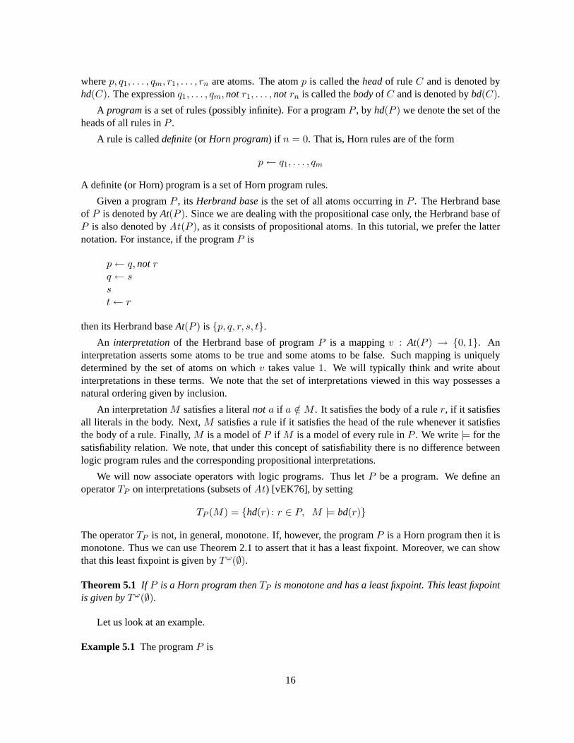
wherep, q1, . . . , qm, r1, . . . , rn are atoms. The atomp is called theheadof ruleC and is denoted byhd(C). The expressionq1, . . . , qm,not r1, . . . ,not rn is called thebodyof C and is denoted bybd(C).
A programis a set of rules (possibly infinite). For a programP , by hd(P ) we denote the set of theheads of all rules inP .
A rule is calleddefinite(or Horn program) if n = 0. That is, Horn rules are of the form
p← q1, . . . , qm
A definite (or Horn) program is a set of Horn program rules.
Given a programP , its Herbrand baseis the set of all atoms occurring inP . The Herbrand baseof P is denoted byAt(P ). Since we are dealing with the propositional case only, the Herbrand base ofP is also denoted byAt(P ), as it consists of propositional atoms. In this tutorial, we prefer the latternotation. For instance, if the programP is
p← q, not rq ← sst← r
then its Herbrand baseAt(P ) is {p, q, r, s, t}.
An interpretationof the Herbrand base of programP is a mappingv : At(P ) → {0, 1}. Aninterpretation asserts some atoms to be true and some atoms to be false. Such mapping is uniquelydetermined by the set of atoms on whichv takes value1. We will typically think and write aboutinterpretations in these terms. We note that the set of interpretations viewed in this way possesses anatural ordering given by inclusion.
An interpretationM satisfies a literalnot a if a /∈ M . It satisfies the body of a ruler, if it satisfiesall literals in the body. Next,M satisfies a rule if it satisfies the head of the rule whenever it satisfiesthe body of a rule. Finally,M is a model ofP if M is a model of every rule inP . We write|= for thesatisfiability relation. We note, that under this concept of satisfiability there is nodifference betweenlogic program rules and the corresponding propositional interpretations.
We will now associate operators with logic programs. Thus letP be a program. We define anoperatorTP on interpretations (subsets ofAt) [vEK76], by setting
TP (M) = {hd(r) : r ∈ P, M |= bd(r)}
The operatorTP is not, in general, monotone. If, however, the programP is a Horn program then it ismonotone. Thus we can use Theorem 2.1 to assert that it has a least fixpoint.Moreover, we can showthat this least fixpoint is given byTω(∅).
Theorem 5.1 If P is a Horn program thenTP is monotone and has a least fixpoint. This least fixpointis given byTω(∅).
Let us look at an example.
Example 5.1 The programP is
16
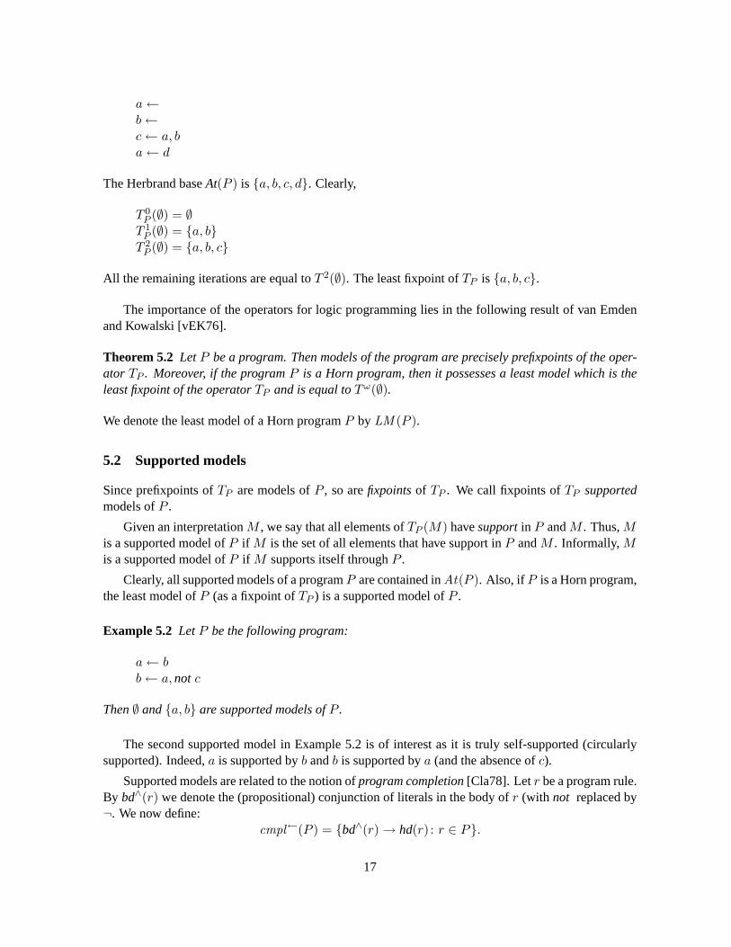
a←b←c← a, ba← d
The Herbrand baseAt(P ) is {a, b, c, d}. Clearly,
T 0P (∅) = ∅T 1P (∅) = {a, b}T 2P (∅) = {a, b, c}
All the remaining iterations are equal toT 2(∅). The least fixpoint ofTP is {a, b, c}.
The importance of the operators for logic programming lies in the following result of van Emdenand Kowalski [vEK76].
Theorem 5.2 LetP be a program. Then models of the program are precisely prefixpoints of the oper-ator TP . Moreover, if the programP is a Horn program, then it possesses a least model which is theleast fixpoint of the operatorTP and is equal toTω(∅).
We denote the least model of a Horn programP by LM (P ).
5.2 Supported models
Since prefixpoints ofTP are models ofP , so arefixpointsof TP . We call fixpoints ofTP supportedmodels ofP .
Given an interpretationM , we say that all elements ofTP (M) havesupportin P andM . Thus,Mis a supported model ofP if M is the set of all elements that have support inP andM . Informally,Mis a supported model ofP if M supports itself throughP .
Clearly, all supported models of a programP are contained inAt(P ). Also, if P is a Horn program,the least model ofP (as a fixpoint ofTP ) is a supported model ofP .
Example 5.2 LetP be the following program:
a← bb← a,not c
Then∅ and{a, b} are supported models ofP .
The second supported model in Example 5.2 is of interest as it is truly self-supported (circularlysupported). Indeed,a is supported byb andb is supported bya (and the absence ofc).
Supported models are related to the notion ofprogram completion[Cla78]. Letr be a program rule.By bd∧(r) we denote the (propositional) conjunction of literals in the body ofr (with not replaced by¬. We now define:
cmpl←(P ) = {bd∧(r)→ hd(r) : r ∈ P}.
17
Thus,cmpl←(P ) is nothing else but a theory obtained by interpreting program rules as propositionalimplications.
We will view all rules inP with the heada as a defnition ofa (listing all cases whena is true).Thus, we define
def P (a) =∨
{bd∧(r) : hd(r) = a}
to denote a formula defininga. From this perspective, ifa holdsdef P (a) must hold too. This iscaptured by the formula
cmpl→(P ) = {a→ def P (a) : a ∈ At}
Thus, to capture a programP in propositional logic we could use the theory
cmpl(P ) = cmpl←(P ) ∪ cmpl→(P )
This theory is known as thecompletionof P [Cla78]. We have the following result connection thecompletion with supported models [MS92].
Theorem 5.3 Let P be a program. A setM ⊆ At is a supported model ofP if and only ifM is amodel ofcmpl(P ).
In particular, it follows that supported models of a program can be computed by SAT solvers.
5.3 Stable model semantics
Stable model semantics [GL88] is one of the most commonly accepted semantics for logic programswith negation. In this section, we will introduce this notion and describe some of its mostimportantproperties.
Let P be a propositional logic program over a set of atomsAt. LetM ⊆ At(P ). By theGelfond-Lifschitz reduct ofP with respect toM , denoted byPM , we mean the logic program obtained fromPby:
1. removing fromP all rules with a literalnot a in the body for somea ∈M
2. removing all negative literals from all other rules inP .
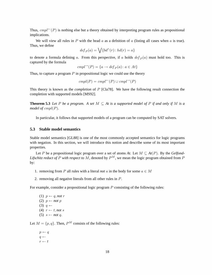
For example, consider a propositional logic programP consisting of the following rules:
(1) p← q, not r(2) p← not p(3) q ←(4) r ← t,not s(5) s← not q.
LetM = {p, q}. Then,PM consists of the following rules:
p← qq ←r ← t
18
The rulep ← not p is eliminated becausep ∈ M . Similarly, rules ← not q is eliminated becauseq ∈M . Since all negative literals in all the remaining rules are of the formnot a for somea /∈M , therules are not eliminated but their negative literals are!
Clearly, for every logic programP and for every set of atomsM , PM is a Horn program. Conse-quently, this logic program has its least modelLM (PM ).
Definition 5.1 We say that a set of atomsM is a stable modelof a propositional logic programP ifM = LM (PM ).
From this definition it is not at all clear that ifM is a stable model ofP then it is a model. This is,however, the case.
Proposition 5.4 If M is a stable model of a logic programP , thenM is a model ofP . Moreover,Mis a minimal model ofP .
Let us look again at programP consisting of rules (1) - (5). ForM = {p, q}, the reductPM isdescribed above and it is clear thatLM (PM ) = M . Hence,M = {p, q} is a stable model ofP . Onthe other hand,M = {q, r} is not. Indeed. in this case,PM consists of
p←q ←r ← t
The least model ofPM is {p, q}. Since it is different fromM = {q, r},M is not a stable model.
Next, we observe that stable models are supported.
Proposition 5.5 If M is a stable model of a logic programP , thenM is a supported model ofP .
The converse is not true in general. We have seen that{a, b} is a supported model of the programPfrom Example 5.2. Clearly,P {a, b} consists of the rulesa ← b andb ← a. Its least model is∅ and itis different from{a, b}. Thus,{a, b} is not a stable model ofP .
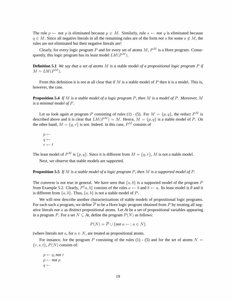
We will now describe another characterizations of stable models of propositional logic programs.For each such a program, we defineP to be a Horn logic program obtained fromP by treating all neg-ative literalsnot a as distinct propositional atoms. LetAt be a set of propositional variables appearingin a programP . For a setN ⊆ At, define the programP (N) as follows:
P (N) = P ∪ {not a← : a ∈ N}
(where literalsnot a, for a ∈ N , are treated as propositional atoms.
For instance, for the programP consisting of the rules (1) - (5) and for the set of atomsN ={r, s, t}, P (N) consists of:
p← q, not rp← not pq ←
19
r ← t,not ss← not qnot r ←not s←not t←
It is easy to see that the least model of this program is
LM (P (N)) = {p, q, not r, not s,not t}.
Its “positive” part,{p, q}, as we saw earlier, is a stable model ofP , and it is also a “complement” ofthe “negative” part{not r, not s,not t} of LM (P (N)). It is not coincidental. We have the followingresult.
Theorem 5.6 LetP be a propositional logic program and let At be the set of atoms appearing inP . AsetM ⊆ At is a stable model ofP if and only ifM ∪ {not a : a ∈ At \M} is the least model of theHorn programP (At \M).
Next, we describe some simple properties of stable model semantics. First, we will show that stablemodel semantics extends the least model semantics for Horn programs.
Proposition 5.7 If P is a Horn program thenP has exactly one stable model. It coincides with theleast model ofP , LM (P ).
Next, we observe that the operator
GLP (M) = LM (PM )
(theGelfond-Lifschitz operator) is antimonotone. That is, ifM1 ⊆M2 then
GLP (M2) ⊆ GLP (M1).
Hence (Theorem 2.3), we have the following result.
Proposition 5.8 Let P be a logic program. Then, the family of its stable models forms an antichainwith respect to inclusion.
Our results on stable models for logic programs parallel, in many cases, the results on extensionsof default theories. This is not coincidental. Logic programming with stable model semantics can beregarded as a special case of default logic.
A default interpretationof a logic program rule
C = p← q1, . . . , qm,not r1, . . . ,not rn
is the defaultdl(C) =
q1 ∧ . . . ∧ qm : ¬r1, . . . ,¬rnp
.
By thedefault interpretationof a logic programP we mean the default theory(dl(P ), ∅), where
dl(P ) = {dl(C) : C ∈ P}.
We have the following result relating logic programming and default logic.
20
Theorem 5.9 LetP be a logic program. A set of atomsM is a stable model forP if and only ifCn(M)is an extension of(dl(P ), ∅). Conversely, every extension of(dl(P ), ∅) is of the formCn(M), for somestable modelM for P .
We have a similar connection to autoepistemic logic. We interpret a ruleC given above by thefollowing modal formula:
ael(C) = ¬Kr1 ∧ . . . ∧ ¬Krn ⊃ (q1 ∧ . . . ∧ qm ⊃ p)
By theautoepistemic interpretationof a logic programP we mean the modal theoryael(P ), where
ael(P ) = {ael(C) : C ∈ P}.
For an modal theoryE, we denote byAt(E) the set of propositional atoms inE.
Theorem 5.10 LetP be a logic program. A setM ⊆ At is a stable model ofP if and only if there isan expansionE of ael(P ) such thatM = At(E).
5.4 Well-founded semantics
We will now describe the so-called well-founded semantics of a program [VRS91].
Let P be a propositional program. We will consider the operatorGLP whose fixpoints are stablemodels ofP . We recall thatGLP (M) = LM (PM ). As we observed in Section 5.3, the operatorGLP is antimonotone. Thus, its second iteration,GL2
P is a monotone operator. According to Theorem2.2, the operatorGL2
P possesses a least fixpoint. We will denote it byT (P ). We also writeM(P ) =GLP (T (P )). One can check thatM(P ) is the largest fixpoint ofGL2
P . These fixpoints oscillate, thatis,
GLP (T (P )) = M(P ) and GLP (M(P )) = T (P ).
Moreover, all the fixpoints ofGLP (stable models) includeT (P ) and are themselves included inM(P ).Thus the least fixpoint ofGL2
P approximates from below the intersection of all stable models, whereasthe largest fixpoint approximates from above the union of stable models ofP . It is important to see thatthe approximation is all we get.
Example 5.3 Let P be this program
p← not qq ← not (p)
The least fixpoint ofGL2P is empty set, whereas the largest fixpoint is{p.q.r}. The intersection of all
stable models is{r} and the union of all stable models is{p, q, r}.
Well-founded semantics is three valued. Atoms inT (P ) are interpreted astrue, atoms inM(P ) areinterpreted aspossiblytrue, and atoms not inM(P ) (we will denote the set of such atoms byF (P ))are interpreted asfalse.
21
5.5 Complexity
Stable model semantics has a major drawback. It is computationally complex [MT91].
Theorem 5.11 The following problems are NP-complete:
1. Given a finite propositional logic programP , decide whetherP has a stable model
2. Given a finite propositional logic programP and an atoma, decide whether there is a stablemodelM of P such thata ∈M
The following problem is co-NP-complete:
3 Given a finite propositional logic programP and an atoma, decide whethera is in all stablemodels ofP
This theorem remains true even under fairly restrictive conditions imposed onthe rules. For in-stance, the assertion remains true for the class of programs in which each rule has no positive atomsand at most one negative literal in the body.
In contrast, well-founded semantics has very good computational properties. In fact, the algorithmfollows directly from the definition of well-founded semantics. First, let us recall that the least model ofa finite propositional Horn program can be computed in timeO(size(P )), wheresize(P ) denotes thetotal length of all rules inP . Consequently, given a finite propositional logic programP and a subsetM of the set of atoms appearing inP , GLP (M) can be computed in timeO(size(P )). According tothe definition of well-founded semantics, setsT andF can be computed by iterating the operatorGLPstarting with the empty set of atoms. Every two iterations the head of at least one ruleis added toT ,or the computation stops. So, the computation terminates inO(|P |) iterations. Thus, we obtain thefollowing result.
Theorem 5.12 There is an algorithm that, given a finite propositional logic programP , computes thewell-founded semantics forP in timeO(|P | × size(P )), where|P | denotes the number of rules inPandsize(P ) denotes the total length of all rules inP .
For more details on well-founded semantics computation we refer to [BSJ95, LT00].
5.6 Stratification and splitting
The efficiency of stable model computation can be improved by exploiting the concept of stratification.While most of the concepts presented in this section can be generalized to the infinite case, we willrestrict our discussion to the case of finite propositional programs.
Let P be a logic program. LetP1, . . . , Pk be nonempty disjoint subprograms ofP such thatP1 ∪. . . ∪ Pk = P . We say thatP1, . . . , Pk is a relaxed stratificationof P if for every 1 ≤ i < j ≤ k,V ar(Pi) ∩ hd(Pj) = ∅. Given a relaxed stratification of a logic programP , we will compute stablemodels forP by computing stable models forP1, then extending them to stable models ofP1 ∪ P2,then extending them to stable models ofP1 ∪ P2 ∪ P3, and so on. The intuitive explanation of the
22
correctness of this method rests on an observation that in iterationi we can only determine the statusof the heads of the rules inPi, and they have no effect on the semantics ofP1 ∪ . . . ∪ Pi−1. Now, wehave the following result.
Theorem 5.13 LetP1, P2 be relaxed stratification of a logic programP . A set of atomsM is a stablemodel forP if and only if there is a subsetM1 ofM such that
1. M1 is a stable model ofP1
2. M is a stable model ofP2 ∪M1
This theorem can be extended by induction to the case of arbitrary relaxed stratifications.
The role of this theorem in stable model computation is now clear. It allows us to replace the taskof computing stable models forP with similar tasks but for simpler programsP1 andP2 ∪M , whereM is a stable model forP1. This leads to substantial pruning of the search space.
This theorem also implies a stronger result for the class ofstratifiedprograms. A relaxed stratifica-tion P1, . . . , Pk of a logic programP is astratificationof P if for eachi, and for each atoma, if not aappears in the body of a rule fromPi thena does not appear as the head of a rule fromPi.
While every programP has relaxed stratification, there are programs that do not admit stratification.Stratified programs can be viewed as an extension of Horn programs, which allows for the use ofnegation in the body of rules but preserves some key properties of Horn programs.
Theorem 5.14 LetP be stratified logic program. ThenP has a unique stable model and this modelcan be computed in timeO(size(P )).
5.7 Tight programs, Fages lemma
We noted that stable models are supported but the converse is not true in general. We will now presenta syntactic condition on programs that guarantees which guarantees that supported models as stable.The results we present here are due to Fages [Fag94], and Erdem and Lifschitz [EL03].
We define apositive dependency graphG+(P ) for a programP as follows. Elements ofAt(P ) asthe vertices ofG+(P ), and(a, b) is an edge inG+(P ) if for somer ∈ P , hd(r) = a, andb ∈ bd+(r)(bd+ (r) is the set of non-negated atoms in the body ofr). A programP is tight if G+(P ) is acyclic.Alternatively, a programP is tight if there is a labeling of atoms with non-negative integers (a 7→ λ(a))s.t. for every ruler ∈ P
λ(hd(r)) > max{λ(b) : b ∈ bd+(r)}
Theorem 5.15 If a programP is tight then every supported model is stable.
The assmption of tightness can be relaxed. LetX ⊆ At(P ). Then,P is tight onX if the programconsisting of rulesr ∈ P such thatbd+(r) ⊆ X is tight.
Theorem 5.16 LetP be a logic program. IfP is tight onX andM is a supported model ofP suchthatM ⊆ X, thenM is stable.
23
We noted that SAT solvers can be used to compute supported models of programs as they aremodels of the completion of the program. The results we presented here allow us, insome cases, tocompute stable models by means of SAT solvers. Clearly, there is no problem if theinput program istight — stable and supported models coincide, so models of the completion are stable,
If the input program is not tight, but is tight onX, we can run a SAT solver on the theorycmpl(P )∪{¬a : a /∈ X}. If this theory has a model, it is a stable model ofP . This method is effective if we areonly interested in stable models of a program that are contained in some setX on whichP is tight.
5.8 Loop formulas
Loop formulas were introduced in [LZ02]. They allow us to transform a logicprogram into a propo-sitional theory so that stable models correspond to models. This transformation is the basis of highlyeffective algorithms for computing stable models that utilize SAT solvers and take advantage of ma-jor advances in SAT technology that have taken place in recent years (we refer tohttp://www.satlive.org/ for a wealth of information on the topic and relevant references). In presenting loopformulas and their properties, we follow [FLL06].
Let P be a logic program andY ⊆ At(P ). We define theexternal support formula forY as thedisjunction of all formulasbd∧(r), wherer ∈ P satisfies:
1. hd(r) ∈ Y
2. bd+(r) ∩ Y = ∅.
The external support formula forY captures the following idea: ifY is to be a part of a stable model,Y must not be self-supported through positive recursion. To put it more formally, there must be at leastone elementa ∈ Y with positive support outside ofY , that is, with a ruler ∈ P such thata = hd(r)andbd+(r) ∩ Y = ∅.
We note thatESP (∅) = ⊤ (the emptyset is always externally supported). We also observe thatESP ({a}) = defP (a). In other words, the external support formula for a singleton set is the same asthe defining formula for its element.
We now have the following theorem.
Theorem 5.17 LetP be a logic program. The following conditions are equivalent:
1. X is a stable model ofP
2. X is a model ofcmpl←(P ) ∪ {Y ∧ → ESP (Y ) : Y ⊆ At(P )}
3. X is a model ofcmpl←(P ) ∪ {Y ∨ → ESP (Y ) : Y ⊆ At(P )}
4. X is a model ofcmpl(P ) ∪ {Y ∧ → ESP (Y ) : Y ⊆ At(P )}
5. X is a model ofcmpl(P ) ∪ {Y ∨ → ESP (Y ) : Y ⊆ At(P )}
To see why (2) and (3) are equivalent to (4) and (5), respectively,we note that
cmpl→(P ) ⊆ {Y ∧ → ESP (Y ) : Y ⊆ At(P )}
24
andcmpl→(P ) ⊆ {Y ∨ → ESP (Y ) : Y ⊆ At(P )}
This result gives a first representation of programs as propositional theories. However, it is clearthat cmpl←(P ) ∪ {Y ∧ → ESP (Y ) : Y ⊆ At(P )} (and all other theories given in the theorem) areexponential in the size ofP . Thus, we do not have yet an effective way to compute stable models withSAT solvers.
To improve Theorem 5.17, we restrict the class of setsY ⊆ At(P ), for which the formulasY ∧ →ESP (Y ) (or Y ∨ → ESP (Y )) need to be added tocmpl←(P ).
Definition 5.2 A loop is a setY ⊆ At(P ) that induces inG+(P ) a strongly connected subgraph
We note that, in particular, all singleton sets are loops. Formulas of the form{Y ∧ → ESP (Y ) areconjunctiveloop formulas, Formulas of the form{Y ∨ → ESP (Y ) aredisjunctiveloop formulas,
Theorem 5.18 LetP be a logic program. The following conditions are equivalent:
1. X is a stable model ofP
2. X is a model ofcmpl←(P ) ∪ {Y ∧ → ESP (Y ) : Y – a loop}
3. X is a model ofcmpl←(P ) ∪ {Y ∨ → ESP (Y ) : Y – a loop}
4. X is a model ofcmpl(P ) ∪ {Y ∧ → ESP (Y ) : Y – a loop}
5. X is a model ofcmpl(P ) ∪ {Y ∨ → ESP (Y ) : Y – a loop}
This theorem shows hat stable models can be computed as models of smaller propositional theories.However, even under the restriction to loops, the size may be exponential in the size ofP . The keyto more practical algorithms is an observation [LZ02] that loop formulas can be added incrementally.We start a SAT solver on the theorycmpl(P ). When a model is found, it is a supported model ofP .If it is stable, we are done. If it is not stable, it gives rise to a loop formula that is not satisfied by it.We add this loop formula and start the SAT solver again. We continue until we finda stable modelor the program terminates without finding models. Here also, in the worst case,we may need to addexponentially many loop formulas before we terminate. However, in many practical situations, thereare either few loops or a stable model is found only after just a small number of loop formulas areadded.
5.9 Strong and uniform equivalence of programs
It is commonly accepted that modular program (or knowledge base) design isa fundamental to facilitatedevelopment, verification and maintenance. For instance, to improve performance, one might want tofocus on a single module and replace its present implementation with an optimized one,before movingon to the next module. However, it is important that the replacement does not change the overallmeaning of the program or knowledge base. Thus, deciding when two programs (or knowledge basesareequivalent for substitutionis a fundamental problem in or declarative programming and knowledgerepresentation.
25
If a knowledge base is a theory in propositional logic, equivalence for substitution coincides withthe standard logical equivalence: theoriesP andQ are equivalent for substitution if and only if theyare logically equivalent.
In nonmonotonic logics, the situation is more complex. In particular, in logic programming withthe semantics of stable models [GL88], having the same stable models does not guarantee equivalencefor substitution. Before we demonstrate this, we will formally define the notion. Following [LPV01],where it was introduced, we use the termstrong equivalenceinstead ofequivalence for substitution.
Definition 5.3 Logic programsP andQ are strongly equivalentif for every logic programR, P ∪ RandQ ∪R have the same stable models.
To show that standard nonmonotonic equivalence (having the same stable models) is not enough toensure strong equivalence, let us consider programs:
P = {p} and Q = {p← not (q)}.
They the same stable models (each program has{p} as itsonly stable model). However,P ∪ {q} andQ ∪ {q} havedifferentstable models. The only stable model ofP ∪ {q} is {p, q} and the only stablemodel ofQ∪{q} is{q}. Similarly,P∪{q ← not (p)} has one stable model,{p}, andQ∪{q ← not (p)}has two stable models{p} and{q}.
[LPV01] presented a characterization of strong equivalence of nested logic programs by exploitingproperties of the logichere-and-there[Hey30]. [Tur01, Lin02, Tur03] continued these studies and ob-tained simple characterizations of strong equivalence in terms ofse-models, without explicit referencesto the logichere-and-there.
[EF03] introduced one more notion of equivalence, theuniform equivalenceof logic programs withanswer-set semantics.
Definition 5.4 Logic programsP andQ are uniformly equivalentif for every setR of facts, P ∪ RandQ ∪R have the same stable models.
[EF03] presented a characterization ofuniform equivalencein terms ofse-modelsand then, forfinite programs, in terms ofue-models, which are se-models with some additional properties.
We will now present key notions and results. First, given a programP we say that a pair(X,Y ),with X,Y sets of atoms, is anse-modelof P if
1. X ⊆ Y
2. Y |= P
3. X |= P Y .
We denote bySE(P ) the set of all se-models ofP . The following characterization is due to Turner[Tur03].
Theorem 5.19 ProgramsP andQ are strongly equivalent if and only ifSE(P ) = SE(Q).
26
Se-models can also be used to characterize uniform equivalence. The following result comes from[EF03].
Theorem 5.20 LetP andQ be programs. ThenP andQ are uniformly equivalent if and only if
1. for everyY ⊆ At,Y is a model ofP if and only ifY is a model ofQ
2. for every(x, y) ∈ SE(P ) such thatX ⊂ Y , there isU ⊆ At such thatX ⊆ U ⊂ Y and(U, Y ) ∈ SE(Q)
3. for every(x, y) ∈ SE(Q) such thatX ⊂ Y , there isU ⊆ At such thatX ⊆ U ⊂ Y and(U, Y ) ∈ SE(P )
For finite programs we have a simpler characterization. An se-model(X,Y ) of P is aue-modelofP if for everyU such thatX ⊂ U ⊆ Y , (U, Y ) ∈ SE(P ) impliesU = Y . We writeUE(P ) for theset of ue-models ofP .
Theorem 5.21 Finite programsP andQ are uniformly equivalent if and only ifUE(P ) = UE(Q).
We note that all these results have extensions to the case of disjunctive logicprograms (in fact, evengeneral logic programs). We also note that it is coNP-complete to decide strong equivalence or uniformequivalence for normal (non-disjunctive) logic programs. When we move up to disjunctive programs,the complexity of deciding strong equivalence remains the same but the complexity of deciding uniformequivalence goes up toΠP
2 -complete.
5.10 General logic programs
In this section, we follow [FL05]. All results we provide come from that paper. We also refer to[LTT99] for a slightly different perspective (closely related but, in some aspects, more general).
Formulasare build from atoms and the symbol⊥ (“false”) by means of the connectives∧, ∨ and→. Thus, the language with which we work here is arestrictedlanguage of propositional logic. Weintroduce other connectives as shorthands:
1. ¬F ::= F → ⊥
2. ⊤ ::= ⊥ → ⊥
3. F ↔ G ::= (F → G) ∧ (G→ F )
As in other places, we consider sets of atoms as interpretations and define thesatisfiability relation|=in a standard propositional logic way.
An occurrence of an atoma in a formulaF is positive, if the number of implications containingthis occurrence ofa in the antecedent is even. Otherwise, it isnegative. An occurrence ofa in F isstrictly positiveif no implication contains this occurrence ofa in the antecedent. In particular,¬F ,being actuallyF → ⊥ has no strict occurrences of any atom.
We will be interested here in thestable-modelsemantics of theories in the language we described.To this end, we define first the notion of thereduct.
27
Definition 5.5 Thereductof a formulaF with respect to a setX of atoms is the formulaFX obtainedby replacing inF each maximal subformula ofF that is not satisfied byX with⊥.
Example 5.4 LetF = (¬p→ q) ∧ (¬q → p) andX = {p}. We observe that:
1. ¬p = p→ ⊥, andX |= ¬p→ q. Thus,¬p is a maximal subformula not satisfied byX
2. ¬q = q → ⊥,X 6|= q,X |= ¬q. Thus,q is a maximal subformula not satisfied byX
Thus,FX = (⊥ → q) ∧ ((⊥ → ⊥)→ p). It is classically equivalent top.
The following properties facilitate the computation of the reduct:
1. ⊥X = ⊥
2. Fora an atom, ifa ∈ X, aX = a; otherwise,aX = ⊥
3. If X |= F ◦G, (F ◦G)X = FX ◦GX ; otherwise,(F ◦G)X = ⊥ (◦ stands for any of∧, ∨,→)
4. If X |= F , (¬F )X = ⊥; otherwise,(¬F )X = (F → ⊥) = (⊥ → ⊥) = ⊤.
Now, we define stable models.
Definition 5.6 LetF be a formula. A setX of atoms is astable modelof a formulaF if X is a minimalmodel ofF .
One can verify that stable models of a programP (according to the original definition) coincidewith stable models (according to this definition) of the representation ofP as the conjunction of theimplications corresponding to its rules:
∧
{cmpl←(r) : r ∈ P}. Thus, the language of propositionalformulas can be regarded as a generalization of logic programs (assuming for each formalism we usethe corresponding stable-model semantics).
We note the following properties of the formalism of general logic programs that extend the familiarproperties we discussed earlier. First, we define an atoma to be aheadatom of a formulaF if at leastone occurrence ofa in F is strictly positive.
Theorem 5.22 If X is a stable model of a formulaF thenX consists of head atoms ofF .
Theorem 5.23 A Horn theory (conjunction of definite Horn clauses given as implications)F has aunique stable model. It is the least model ofF .
Formulas of the form¬F areconstraints.
Theorem 5.24 A setX is a stable model of a formulaF ∧ ¬G if and only ifX is a stable model ofFandX |= ¬G.
We say that a formulaF is strongly equivalent to a formulaF ′ if for every formulaG, F ∧G andF ′ ∧G have the same stable models.
We say that(X,Y ) is anse-modelof F if Y ⊆ At,X ⊆ Y , Y |= F andX |= F Y .
28
Theorem 5.25 The following conditions are equivalent:
1. FormulasF andG are strongly equivalent
2. For every setX of atoms,FX andGX are equivalent in classical logic
3. F andG have the same se-models
4. F andG are equivalent in the logic here-and-there (details later)
Finally, we mention a generalization of the splitting theorem.
Theorem 5.26 LetF andG be formulas such thatF does not contain any of the head atoms ofG. AsetX is a stable model ofF ∧ G if and only if there is a stable modelY of F such thatX is a stablemodel ofG ∧
∧
Y .
6 Modal Logics and Modal Nonmonotonic Logic S4F
In this section, we follow [Tru07]. Our overall goal in this section is to show that nonmonotonic modallogic S4F can be regarded as central to nomonotonic reasoning. We start with a brief overview of basicconcepts related to modal logics and modal nonmonotonic logics.
We refer to [HC84, MT93a] for a detailed discussion of topics related to modal logics and a generaldiscussion of modal nonmonotonic logics. We consider the propositional modal language determinedby a setAt (possibly infinite) of propositional atoms, a constant⊥, the usual boolean connectives¬,∨, ∧,→, and a single modal operatorK. The constant⊥ represents a “generic”contradictionandKis read as “known”. An inductive definition of a formula, given in the BNF notation, is as follows:
ϕ ::= ⊥ | p |Kϕ | ¬ϕ |ϕ ∨ ϕ |ϕ ∧ ϕ |ϕ→ ϕ,
wherep ∈ At . We denote the language consisting of such formulas byLK (we drop references toAt
from the notation as it is fixed). We writeL for the set ofK-free (modal-free) formulas inLK .
Modal logics differ in the properties of the modalityK. A modal logicS is defined semanticallyby its entailmentrelation|=S , specified byKripke interpretations, or proof-theoretically by means ofproofs based on a set of modal axioms ofS.
Let S be a modal logic with the entailment relation|=S . For every theoryI ⊆ LK , a theoryT ⊆ LK is anS-expansionof I [MD80, McD82] if
T = {ϕ ∈ LK : I ∪ ¬KT |=S ϕ},
where¬KT = {¬Kϕ : ϕ ∈ LK \ T}. The nonmonotonic logicS is a formalism, in which thesemantics of a theoryI ⊆ LK is given by itsS-expansions. This definition coincides with the one wegave earlier, which relied on the equivalent proof-theoretic presentation of modal logics that used theconsequence operatorCnS .
If A ⊆ L is a propositional theory thenA has auniqueS5-expansion, where S5 is a well-knownmodal logic whose entailment relation is given by Kripke interpretations with the universal accessibilityrelation. According to Proposition 4.2, this unique expansion is given by
CnS5(A ∪ {¬Kϕ : ϕ ∈ L \A})
29
We will denote this unique expansion byST(A)1. We use this notation in the following result, whichgives us a way to represent expansions.
Theorem 6.1 If S is a modal logic contained in S5 andA ⊆ L, then ST(A) is the uniqueS-expansionofA. Moreover, for everyT ⊆ LK , if E is anS-expansion ofT , thenE = ST(A), whereA = E ∩ L.
6.1 Logic S4F
The modal logicS4F is fundamental to nonmonotonic reasoning [Seg71, Voo91, MT93a, ST94]. Thenonmonotonic logicS4F captures, under some direct and intuitive encodings [Tru91a, ST94],the (dis-junctive) logic programming with the stable-model (answer-set) semantics [GL91], the (disjunctive)default logic [Rei80, GLPT91], the logic of grounded knowledge [LS90], the logic of minimal beliefand negation as failure [Lif94] and the logic of minimal knowledge and belief [ST94].
The logicS4F is a modal logic with the semantics given byKripkeS4F-interpretations(or simply,S4F-interpretations), that is, tuples〈V,W, π〉, where
1. V andW arenonemptyand disjoint sets ofworlds, and
2. π is a function assigning to each worldw ∈ V ∪W a set of atomsπ(w), representing aproposi-tional truth valuation forw.
Given anS4F-interpretationM = 〈V,W, π〉, we define thesatisfaction relationM, w |= ϕ, wherew ∈ V ∪W andϕ ∈ LK , as follows:
1. M, w 6|= ⊥
2. M, w |= p if p ∈ π(w) (for p ∈ At)
3. If w ∈ V , thenM, w |= Kϕ if M, v |= ϕ for everyv ∈ V ∪W
4. If w ∈W , thenM, w |= Kϕ if M, v |= ϕ for everyv ∈W
5. The induction over boolean connectives is standard. For instance,M, w |= ϕ ∧ ψ if M, w |= ϕandM, w |= ψ.
An S4F-interpretationM = 〈V,W, π〉 is anS4F-model ofϕ ∈ LK , writtenM |= ϕ, if for everyw ∈ V ∪W ,M, w |= ϕ. We writeϕ |=S4F ψ if every S4F-model ofϕ is anS4F-model ofψ. Thenotation extends in a standard way tomodal theories, that is, subsets ofLK . We note that|=S4F has aproof-theoretic characterization based on the necessitation inference ruleand axiom schemata K, T, 4and F [Seg71, MT93a].
From now on we focus on the nonmonotonic logicS4F. We start with a result characterizingS4F-expansions (a slight restatement of a result from [Sch92b]). For anS4F-interpretationM = 〈V,W, π〉,we writeLM (UM) for the set of all formulas fromL (propositional formulas) that hold in every truthassignmentπ(v), wherev ∈ V (π(w), wherew ∈W , respectively).
1The notation reflects the fact that expansions arestable theories [Sta80, McD82], cf. also our earlier discussion ofautoepistemic logic.
30
Theorem 6.2 Let I ⊆ LK . A theoryT ⊆ LK is anS4F-expansion ofI if and only if there is anS4F-modelM of I such thatT = ST(UM); LM = UM; and for everyS4F-modelN of I withUN = UM,UN ⊆ LN .
6.2 Modal defaults
We will now use the nonmonotonic logicS4F to generalize default logic.
A modal defaultis defined inductively (in the BNF notation) as:
ϕ ::= Kψ |Kϕ | ¬ϕ |ϕ ∨ ϕ |ϕ ∧ ϕ |ϕ→ ϕ,
whereψ ∈ L. Informally, modal defaults are built according to standard rules for boolean connectivesandK of formulasKψ, whereψ ∈ L. A modal default theoryis set of modal defaults.
When we restrict to modal defaults and theories the semantics simplifies. AnS4F-pair is a pair〈L,U〉, whereL,U ⊆ L are propositional theories closed under propositional entailment.
For anS4F-pair 〈L,U〉 and a modal defaultϕ, we define two satisfiability relations〈L,U〉 |=l ϕand〈L,U〉 |=u ϕ inductively as follows:
1. Forϕ = Kψ, whereψ ∈ L, we define〈L,U〉 |=u ϕ if ψ ∈ U ; and we define〈L,U〉 |=l ϕ ifψ ∈ L ∩ U
2. We handle boolean connectives in the standard way. For instance, for ϕ = ¬ψ, whereψ is amodal default, we define〈L,U〉 |=u ϕ if 〈L,U〉 6|=u ψ; and〈L,U〉 |=l ϕ if 〈L,U〉 6|=l ψ
3. Forϕ = Kψ, whereψ is a modal default, we define〈L,U〉 |=u ϕ if 〈L,U〉 |=u ψ; and we define〈L,U〉 |=l ϕ if 〈L,U〉 |=l ψ and〈L,U〉 |=u ψ
We write〈L,U〉 |=md ϕ if 〈L,U〉 |=l ϕ and〈L,U〉 |=u ϕ.
If M is anS4F-interpretation then〈LM, UM〉 is anS4F-pair. Also, for everyS4F-pair 〈L,U〉there is anS4F-interpretationM = 〈V,W.π〉 such thatLM = L andUM = U .
There is a close connection between|=S4F and the relations|=l, |=u and|=md.
Proposition 6.3 LetM = 〈V,W, π〉 be anS4F-interpretation andϕ a modal default.
1. For everyv ∈ V :M, v |= ϕ if and only if〈LM, UM〉 |=l ϕ
2. For everyw ∈W :M, w |= ϕ if and only if〈LM, UM〉 |=u ϕ
3. M |= ϕ if and only if〈LM, UM〉 |=md ϕ.
And now we have a simpler characterization ofS4F-expansions that works for modal default theo-ries.
Theorem 6.4 Let I ⊆ LK be a modal default theory. A theoryT ⊆ LK is an S4F-expansion ofI if and only if there isU ⊆ L such thatU is closed under propositional entailment,T = ST(U),〈U,U〉 |=md I, and for everyS4F-pair 〈L,U〉, 〈L,U〉 |=md I impliesU ⊆ L.
31
An se-interpretationis anS4F-pair 〈L,U〉 such thatL ⊆ U . If I is a modal default theory then anse-interpretation〈L,U〉 such that〈L,U〉 |= I is anse-modelof I. It turns out that that for modal defaulttheories se-interpretations suffice to characterize theS4F-entailment. For a modal default theoryI anda modal defaultϕ we writeI |=se ϕ if every se-model ofI is an se-model ofϕ.
Theorem 6.5 Let I ⊆ LK be a modal default theory and letϕ ∈ LK be a modal default. ThenI |=S4F ϕ if and only ifI |=se ϕ.
Corollary 6.6 Let I ⊆ LK be a modal default theory. A theoryT ⊆ LK is anS4F-expansion ofI ifand only if there isU ⊆ L such thatU is closed under propositional entailment,T = ST(U), 〈U,U〉 isan se-model forI, and for every se-model〈L,U〉 for I, U = L.
Let I ⊆ LK . An se-interpretation〈U,U〉 is anse-expansionof I if 〈U,U〉 |= I and for everyse-model〈L,U〉 of I, L = U . Our results show that there is a one-to-one correspondence betweenS4F-expansions and se-expansions.
Corollary 6.7 Let I ⊆ LK be a modal default theory. A theoryT ⊆ LK is anS4F-expansion ofI ifand only if there is an se-expansion〈U,U〉 of I such thatT = ST(U).
6.3 Strong equivalence for the nonmonotonic logic S4F
We will now characterize strong equivalence of modal default theoriesI andI ′ (modal default theoriesI, I ′ are strongly equivalentif for every modal default theoryJ , I ∪ J and I ′ ∪ J have the sameS4F-expansions, or equivalently, the same se-expansions.
Theorem 6.8 Let I, I ′ ⊆ LK be modal default theories. The following conditions are equivalent:
1. I andI ′ are strongly equivalent
2. I andI ′ have the same se-models.
6.4 Uniform equivalence for the nonmonotonic logic S4F
We will use the following notation for a setX of (modal) formulas:KX = {Kϕ : ϕ ∈ X}. LetP,Q ⊆ LK be modal theories. We say thatP andQ areuniformly equivalentif for every setX ⊆ L,P ∪KX andQ ∪KX have the sameS4F-expansions. IfP andQ are modal default theories then foreveryX ⊆ L, P ∪KX andQ∪KX are modal default theories, too. It turns out that se-interpretationscan also be used to characterize uniform equivalence. Namely, we havethe following theorem.
Theorem 6.9 Default modal theoriesP,Q ⊆ LK are uniformly equivalent if and only if the followingthree conditions hold:
1. for every se-interpretation〈U,U〉, 〈U,U〉 |=md P if and only if〈U,U〉 |=md Q
2. for every se-interpretation〈L,U〉, if L ⊂ U and〈L,U〉 |=md P then there is an se-interpretation〈L′, U〉 such thatL ⊆ L′ ⊂ U and〈L′, U〉 |=md Q
32

3. for every se-interpretation〈L,U〉, if L ⊂ U and〈L,U〉 |=md Q then there is an se-interpretation〈L′, U〉 such thatL ⊆ L′ ⊂ U and〈L′, U〉 |=md P
As in the case of logic programs, we can introduce the notion of aue-modeland, derive fromTheorem 6.9 a simpler characterization of uniform equivalence offinitemodal default theories in termsof ue-models.
6.5 Modal programs
We will now considermodal programs, a special class of modal default theories consisting ofmodalrules. As it will become clear later, modal programs are equivalent to general logic programs. The twoformalisms can be viewed as notational invariants of one another.
A formal inductive definition of amodal rule, given in the BNF notation, is as follows:
ϕ ::= Kp |Kϕ | ¬ϕ |ϕ ∨ ϕ |ϕ ∧ ϕ |ϕ→ ϕ,
wherep ∈ At ∪ {⊥}. A modal programis a set of modal rules.
If X ⊆ L, we writeCn(X) for the set of all propositional consequences ofX. A simple se-interpretationis any se-interpretation of the form〈Cn(L), Cn(U)〉, whereL,U ⊆ At . To characterizeS4F-expansions of modal programs it suffices to restrict to simple se-interpretations. Indeed, the fol-lowing results state the key property of modal rules.
Theorem 6.10 If ϕ is a modal rule and〈L,U〉 is an se-interpretation then〈L,U〉 |= ϕ if and only if〈Cn(L ∩At), Cn(U ∩At)〉 |= ϕ.
Corollary 6.11 If I andI ′ are modal programs, thenI andI ′ have the same se-models if and only ifthey have the same simple se-models.
These results allow us to strengthen the characterization of strong equivalence in the case of modalprograms.
Corollary 6.12 Let I, I ′ ⊆ LK be modal programs. The following conditions are equivalent:
1. I andI ′ are strongly equivalent
2. I andI ′ have the same simple se-models.
Using a similar argument we can also strengthen the characterization of the uniform equivalence ofmodal programs (Theorem 6.9) by consistently replacing se-interpretations with simple se-interpretations.
6.6 The Logic Here-and-There
There is a strong connection between simple se-interpretations and models of non-classical proposi-tional logic known as the logichere-and-there[Hey30, Pea97, FL05].
33
We will introduce the logic here-and-there and mention its connection to generallogic programs.We will also note that it can be embedded in the logicS4F.
The language of the logic here-and-there has three primitive binary connectives∧, ∨ and→, anda constant⊥ to represent a generic contradiction (thus, it is the same as the language of general logicprograms). And we use the same shorthands as before.
The semantics of the logic here-and-there is given by HT-interpretations. An HT-interpretationis apair 〈L,U〉, whereL ⊆ U ⊆ At are sets of atoms. We define the satisfiability relation〈L,U〉 |=ht ϕ,whereϕ ∈ Lht , by induction as follows:
1. 〈L,U〉 6|= ⊥
2. Forϕ = p, wherep ∈ At , we define〈L,U〉 |=ht p if p ∈ L
3. 〈L,U〉 |=ht ϕ ∧ ψ if 〈L,U〉 |=ht ϕ and〈L,U〉 |=ht ψ
4. 〈L,U〉 |=ht ϕ ∨ ψ if 〈L,U〉 |=ht ϕ or 〈L,U〉 |=ht ψ
5. 〈L,U〉 |=ht ϕ → ψ if (i) 〈L,U〉 6|=ht ϕ or 〈L,U〉 |=ht ψ; and (ii)U |= ϕ → ψ (in standardpropositional logic).
An HT-interpretation〈U,U〉 is anequilibrium modelof A ⊆ Lht if 〈U,U〉 |=ht A and for everyL ⊆ U , if 〈L,U〉 |=ht A thenL = U [Pea97]. It is easy to see that equilibrium models correspondto stablemodels of general logic programs [FL05] (cf. our earlier discussion). This, there is a directconnection between the two formalisms.
We will now show that the logic here-and-there can be embedded in the logic S4F. To this end, forevery propositional formulaϕ ∈ Lht we define a formulaϕ¬K¬K to be a modal rule obtained fromϕ by replacing eacha ∈ At ∪ {⊥} in ϕ with ¬K¬Ka (intuitively, ¬K¬K represents a modalityexhibiting properties of thebelief modality). We note that all formulasϕ¬K¬K are modal rules.
Next, for every propositional formulaϕ ∈ Lht we define the corresponding modal ruleϕmp induc-tively as follows:
1. amp = Ka for a ∈ At ∪ {⊥}
2. (ϕ ∧ ψ)mp = ϕmp ∧ ψmp and(ϕ ∨ ψ)mp = ϕmp ∨ ψmp
3. (ϕ→ ψ)mp = (ϕmp → ψmp) ∧ (ψ → ϕ)¬K¬K .
We extend this notation to sets of formulas: for a setA ⊆ Lht , we defineAmp = {ϕmp |ϕ ∈ A}.
We have the following result establishing the connection between the logic here-and-there and thelogic S4F.
Theorem 6.13 LetA ⊆ Lht andϕ ∈ Lht . The following conditions are equivalent:
1. A |=ht ϕ
2. Amp |=se ϕmp
3. Amp |=S4F ϕmp .
34
Corollary 6.14 LetA ⊆ Lht andU ⊆ At . The following conditions are equivalent:
1. U is a stable model ofA
2. 〈U,U〉 is an equilibrium model ofA
3. 〈Cn(U), Cn(U)〉 is an se-expansion ofA
4. ST(U) is anS4F-expansion ofAmp .
6.7 Logic of nested defaults
Let α : β1,...,βm
γ1|...|γnbe a disjunctive default [GLPT91]. By encoding it with a modal default
Kα ∧K¬Kβ1 ∧ . . . ∧K¬Kβk → Kγ1 ∨ . . . ∨Kγn
we obtain an embedding of (disjunctive) default theories inLK which establishes a one-to-one corre-spondence between extensions andS4F-expansions [Tru91a]. Thus, the class of modal default theorieswith the semantics ofS4F-expansions (or se-expansions) can be regarded as a generalization of thedisjunctive default logic. In fact, we can regard it as a general default logic of nested defaults as itcovers, for instance, the case of formulas of the form
Kα ∧K¬Kβ1 ∧ . . . ∧K¬Kβk → Kγ1 ∨ . . . ∨Kγn
whereα, βi andγi are arbitrary modal defaults rather than formulas fromL.
We also note that by exploiting the embedding given above, our results on strong equivalenceof modal default theories can be specialized to results on strong equivalence of disjunctive defaulttheories, first obtained by Turner [Tur03]. Our results on uniform equivalence of modal default theoriesgeneralize those obtained by Truszczynski [Tru06].
7 Algebraic approach to nonmonotonic reasoning
This section closely follows [DMT00a],
7.1 Preliminaries from lattice theory
A lattice is a partially ordered set〈L,≤〉 such that every two element set{x, y} ⊆ L has aleast upperbound, lub(x, y), and agreatest lower bound, glb(x, y). A lattice〈L,≤〉 is completeif every subset ofL has both least upper and greatest lower bounds. Consequently, a complete lattice has a least element(⊥) and a greatest element (⊤).
Earlier, we discussed operators on families of sets. Now, we generalize thediscussion to a moreabstract setting. If〈L,≤〉 is a lattice, functions fromL to L areoperatorson the lattice. An operatorO on L is monotoneif for every x, y ∈ L, x ≤ y impliesO(x) ≤ O(y). An operatorO on L isantimonotoneif for everyx ≤ y,O(y) ≤ O(x).
We have the following two simple properties.
35
Proposition 7.1 If the operatorsO1 : L → L, O2 : L → L are antimonotone, then the operatorO1 ◦O2 is monotone.
Proposition 7.2 If an operatorO : L→ L is monotone and antimonotone then it is constant.
Tarski-Knaster theorem [Tar55] also generalizes to the abstract setting of operators on lattices. Anelementx ∈ L is aprefixpointof a lattice operatorL, if O(x) ≤ x, and afixpointof L, if O(x) = x.
Theorem 7.3 LetO be a monotone operator on a complete lattice〈L,≤〉. Then,O has a least prefix-point and a least fixpoint and the two coincide.
We denote the least fixpoint of an operatorO by lfp(O).
An elementz ∈ L is approximatedby a pair(x, y) ∈ L2 if x ≤ z ≤ y. Approximations of theform (x, x) are calledexact. There is a straightforward one-to-one correspondence betweenL and theset of exact elements ofL2.
The setL2 can be given with two orderings. First, thelatticeordering≤ is given by
(x, y) ≤ (x1, y1) if x ≤ x1 and y ≤ y1.
Second, theinformationordering,≤i, which captures the intuition of increased precision of the ap-proximation, is given by
(x, y) ≤i (x1, y1) if x ≤ x1 and y1 ≤ y.
With each of these two orderingsL2 is a complete lattice.
A pair (x, y) ∈ L2 is consistentif x ≤ y. Otherwise, it is calledinconsistent. Consistent pairscan be viewed as descriptions of, in general, incomplete knowledge about elements fromL that theyapproximate. The information ordering when applied to consistent pairs measures their precision, whenapplied to inconsistent pairs measures the “degree of inconsistency”.
The collection of consistent pairs does not form a sublattice ofL2. Indeed, each element of the form(x, x) is a maximal consistent element ofL2. By allowing inconsistent approximations, we obtain aduality between consistent and inconsistent pairs, and between the degreeof precision and the degreeof inconsistency. Consequently, we obtain a richer algebraic structure and a more elegant theory.
A pair of elementsx, y ∈ L is anoscillating pairfor an operatorO onL if y = O(x) andx = O(y).An oscillating pair(x, y) is extremeif for every oscillating pair(x′, y′) for O, (x, y) ≤i (x′, y′) and(x, y) ≤i (y′, x′) (or equivalently,x ≤ x′, y′ ≤ y). If (x, y) is an extreme oscillating pair thenx ≤ y.Moreover, if an extreme oscillating pair exists, it is unique.
Theorem 7.4 LetO be an antimonotone operator on a complete lattice〈L,≤〉. Then,O2 has a leastfixpoint and a greatest fixpoint and(lfp(O2), O(lfp(O2))) is the unique extreme oscillating pair ofO.
LetA be an operator onL2. Let us denote byA1 andA2 the functions fromL2 toL such that
A(x, y) = (A1(x, y), A2(x, y)).
We say thatA is symmetricif A1(x, y) = A2(y, x). If an operatorA : L2 → L2 is symmetric thenfor everyx ∈ L, A1(x, x) = A2(x, x). In the remainder of this document, we consider symmetricoperators only.
36
We now have several useful characterizations and properties of symmetricoperators that are mono-tone wrt≤i and/or≤.
Proposition 7.5 A symmetric operatorA : L2 → L2 is ≤i-monotone if and only if for everyy ∈ L,A1(·, y) is monotone and for everyx ∈ L, A1(x, ·) is antimonotone (or equivalently, if and only if foreveryy ∈ L,A2(·, y) is antimonotone and for everyx ∈ L,A2(x, ·) is monotone).
Proposition 7.6 A symmetric operatorA : L2 → L2 is≤-monotone if and only if for everyx, y ∈ L,A1(x, ·) andA1(·, y) are monotone (or, equivalently, if and only if for everyx, y ∈ L, A2(x, ·) andA2(·, y) are monotone).
Proposition 7.7 An operatorA : L2 → L2 is symmetric and monotone with respect to both≤i and≤ if and only if there is a monotone operatorO : L → L such that for everyx, y ∈ L, A(x, y) =(O(x), O(y)).
Proposition 7.8 An operatorA : L2 → L2 is symmetric,≤i-monotone and≤-antimonotone if andonly if there is an antimonotone operatorO : L → L such that for everyx, y ∈ L, A(x, y) =(O(y), O(x)).
By Propositions 7.7 and 7.8 there is a one-to-one correspondence betweenmonotone (antimono-tone, respectively) operators onL and≤i-monotone and≤-monotone (≤i-monotone and≤-antimonotone,respectively) operators onL2.
WhenL is a complete lattice, Knaster-Tarski Theorem Theorem 7.4 imply that an≤i-monotoneand≤-antimonotone operatorA : L2 → L2 has≤i-least and≤i-greatest fixpoints and a≤-extremeoscillating pair. Let us denote the≤i-least fixpoint ofA by qA, and the≤i-greatest fixpoint ofA byQA. Similarly, let us denote the≤-extreme oscillating pair forA by (eA, EA).
If A : L2 → L2 is, in addition, symmetric, by Proposition 7.8, there is an antimonotone operatorO : L→ L such thatA(x, y) = (O(y), O(x)). Let us denote byq the least fixpoint ofO2 and byQ thegreatest fixpoint ofO2 (Tarski-Knaster Theorem applies asO2 is monotone). The following theorem,due essentially to Fitting, summarizes the relations between the fixpoints and extremepairs definedabove.
Theorem 7.9 Let L be a complete lattice. LetA : L2 → L2 be a symmetric≤i-monotone and≤-antimonotone operator onL2. Then:
1. qA = (q,Q),QA = (Q, q), eA = (q, q), EA = (Q,Q)
2. qA = glb≤i(eA, EA) andQA = lub≤i
(eA, EA)
3. eA = glb≤(qA, QA) andEA = lub≤(qA, QA).
7.2 Approximating operators
Definition 7.1 An operatorA : L2 → L2 extendsan operatorO : L → L if for everyx ∈ L,A(x, x) = (O(x), O(x)). An operatorA : L2 → L2 is extendingif for everyx ∈ L, there isy ∈ Lsuch thatA(x, x) = (y, y).
37
Thediagonalof L2 is the set{(x, x) : x ∈ L} If an operatorA : L2 → L2 extendsO : L → Lthen the behavior ofA on the diagonal determines the behavior ofO.
Proposition 7.10 LetO be an operator on a latticeL and letA be an operator onL2 extendingO.Then,x is a fixpoint ofO if and only if(x, x) is a fixpoint ofA.
If A is symmetric then for each lattice elementx, A1(x, x) = A2(x, x). HenceA(x, x) is exactand, consequently,A is extending.
Proposition 7.11 If an operatorA : L2 → L2 is symmetric thenA is extending.
To study fixpoints of an operatorO one might construct an appropriate extending operatorA andstudy its fixpoints instead. Exact fixpoints of the operatorA provide a description of the fixpoints ofO. A situation is especially interesting ifA is symmetric and≤i-monotone.
Definition 7.2 An operatorA : L2 → L2 approximatesan operatorO : L → L if A is symmetric,extendsO and is≤i-monotone. An operatorA : L2 → L2 is approximatingif it is symmetric and≤i-monotone.
We say that an operatorA : L2 → L2 is consistentif it maps consistent pairs to consistent pairs.
Proposition 7.12 If A : L2 → L2 is an approximating operator, thenA is consistent.
Corollary 7.13 LetA : L2 → L2 be an approximating operator for an operatorO : L→ L. Then,Ahas a≤i-least fixpoint. This fixpoint is consistent and approximates every fixpoint ofO.
If the≤i-least fixpoint of an approximating operatorA for an operatorO is exact, say of the form(x, x), thenx is the only fixpoint ofO. Since in the case of logic programming, the concept of the≤i-least fixpoint of an approximating operator to the operatorTP gives Kripke-Kleene semantics, werefer to the≤i-least fixpoint of an approximating operatorA as theKripke-Kleene fixpointof A. Wedenote this fixpoint byαA.
Let O be a monotone operator onL. By Proposition 7.7, the operatorAO(x, y) = (O(x), O(y))is ≤i-monotone. It is also symmetric, consistent and extends the operatorO. Hence,AO is an ap-proximating operator forO. By Proposition 7.7,AO is ≤-monotone. In fact, Proposition 7.7 impliesthatAO is a unique approximating operator forO that is≤-monotone. The least≤i-fixpoint of AOis (lfp(O), lfp(O)). We will call AO the canonicalapproximating operator for a monotone operatorO. This algebraic property of monotone operators explains why all major nonmonotonic semanticscoincide on the class of Horn theories (or programs) and are given by the least fixpoint construction.
Similarly, if A is an antimonotone operator onL then, by Proposition 7.8, the operatorAO(x, y) =(O(y), O(x)) is≤i-monotone. In addition,AO is symmetric, consistent and it extendsO. Hence, it isan approximating operator forO. By Proposition 7.8,AO is≤-antimonotone and, in fact, it is a uniqueapproximating operator forO that is≤-antimonotone. We will callAO thecanonicalapproximatingoperator for an antimonotone operatorO. Theorem 7.9 characterizes the fixpoints and the extremeoscillating pair of the trivial approximating operator for an antimonotone operator O.
38
7.3 Stable operator and well-founded fixpoint
In this section we describe an algebraic construction that assigns to every≤i-monotone operatorA ona bilatticeL2 its stableoperatorCA defined also onL2.
Definition 7.3 Let L be a complete lattice. Let an operatorA : L2 → L2 on a bilatticeL2 besymmetric and≤i-monotone.
1. Thecomplete stable operator forA, CA : L → L, is defined byCA(y) = lfp(A1(·, y)) (or,equivalently, by,CA(y) = lfp(A2(y, ·))).
2. Thestable operator forA, CA : L2 → L2 is defined byCA(x, y) = (CA(y), CA(x)).
Since for everyy ∈ L the operatorsA1(·, y) andA2(y, ·) are monotone (Proposition 7.5), the operatorsCA andCA are well-defined.
Let us consider an operatorA that is both≤i- and≤-monotone. Such operators are described inProposition 7.7. They are of the formA(x, y) = (O(x), O(y)), whereO is monotone. It follows thatCA(y) = lfp(O) and does not depend ony. Thus, we get the following result.
Proposition 7.14 LetL be a complete lattice. LetA : L2 → L2 be an operator monotone with respectto≤i and≤. ThenCA is constant.
If an operatorA is ≤i-monotone and≤-antimonotone then, by Proposition 7.8, there is an anti-monotone operatorO such thatA(x, y) = (O(y), O(x)). Consequently,A(·, y) = O(y). It followsthatCA(y) = O(y), that is, the stable operator for the operatorA isA itself.
Proposition 7.15 LetL be a complete lattice. LetA : L2 → L2 be an operator monotone with respectto≤i and antimonotone with respect to≤. ThenCA = A.
The next several results establish properties of the stable operatorCA and its fixpoints. Our firstresult shows that fixpoints ofCA are≤-minimal fixpoints ofA.
Theorem 7.16 LetL be a complete lattice. Let an operatorA : L2 → L2 on a bilatticeL2 be≤i-monotone. Every fixpoint of the stable operatorCA is a≤-minimal fixpoint ofA.
Theorem 7.16 shows, in particular, that ifA is≤i-monotone, a fixpoint ofCA is also a fixpoint ofA. We will call every fixpoint of the stable operatorCA astablefixpoint ofA.
Directly from the definition of the operatorsCA and from Proposition 7.5 it follows thatCA isantimonotone. Consequently, by Proposition 7.8,CA is≤i-monotone and≤-antimonotone.
Proposition 7.17 Let L be a complete lattice. LetA be a symmetric≤i-monotone operator onL2.Then,CA is an antimonotone operator onL andCA is a≤i-monotone and≤-antimonotone operatoronL2.
Propositions 7.15 and 7.17 imply the following corollary that states that applying the stability con-struction to a stable operator does not lead to a new operator anymore.
39

Corollary 7.18 LetL be a complete lattice. LetA be a symmetric≤i-monotone operator onL2. ThenCCA = CA.
It is also easy to see thatCA is symmetric and extends the operatorCA. Thus, we obtain thefollowing corollary to Proposition 7.17.
Corollary 7.19 LetL be a complete lattice. LetA be a≤i-monotone operator onL2. Then, the stableoperatorCA is a trivial approximation of the complete stable operatorCA.
The≤i-least fixpoint ofCA is of particular interest as it provides an approximation to every stablefixpoint ofA. We call the≤i-least fixpoint ofCA thewell-founded fixpointof a≤i-monotone operatorAand denote it byβA. The choice of the term is dictated by the fact that in the case of logic programming,the least fixpoint of the stable operator for the 4-valued van Emden-Kowalski operatorTP yields thewell-founded semantics.
The following result gathers several properties of the well-founded fixpoint of an operator thatgeneralize properties of the well-founded model of a logic program.
Theorem 7.20 LetL be a complete lattice. LetA : L2 → L2 be a≤i-monotone symmetric operator.
1. The Kripke-Kleene fixpointαA and the well-founded fixpointβA satisfyαA ≤i βA
2. For every stable fixpointx ofA, βA ≤i x
3. If βA is exact then it is the only consistent stable fixpoint ofA.
4. The operatorCA is consistent and, consequently,βA is consistent, too.
We will now assume thatA is an approximating operator for an operatorO : L → L and discussthe relationship between the fixpoints ofCA and fixpoints ofO.
Proposition 7.21 LetL be a complete lattice. LetA : L2 → L2 be an approximating operator for anoperatorO : L→ L. If (x, x) is a fixpoint ofCA thenx is a≤-minimal fixpoint ofO.
It follows from Proposition 7.21 that ifA is an approximating operator for an operatorO thenfixpoints ofO corresponding to exact fixpoints of the stable operatorCA form an antichain.
We will next consider the case whenO is monotone and use the canonical approximation ofO,AO.
Proposition 7.22 LetL be a complete lattice. IfO : L → L is a monotone operator, then for everyx ∈ L, CAO
(x, y) = (lfp(O), lfp(O)) (that is,CAOis constant).
If O is monotone, its canonical approximationAO may have many fixpoints in general and manyexact fixpoints, in particular. However, by Proposition 7.22, the stable operator forAO has only onefixpoint and it corresponds precisely to the least fixpoint ofO. In the context of logic programming,this result says that a Horn logic programP has a unique stable model and that it coincides with theleast Herbrand model ofP .
40
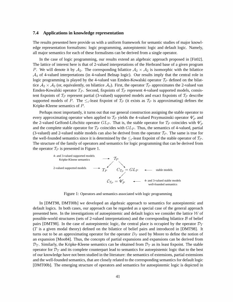
7.4 Applications in knowledge representation
The results presented here provide us with a uniform framework for semantic studies of major knowl-edge representation formalisms: logic programming, autoepistemic logic and default logic. Namely,all major semantics for each of these formalisms can be derived from a singleoperator.
In the case of logic programming, our results extend an algebraic approachproposed in [Fit02].The lattice of interest here is that of 2-valued interpretations of the Herbrand base of a given programP . We will denote it byA2. The corresponding bilatticeA2 × A2 is isomorphic with the bilatticeA4 of 4-valued interpretations (in 4-valued Belnap logic). Our results imply that the central role inlogic programming is played by the 4-valued van Emden-Kowalski operatorTP defined on the bilat-ticeA2 × A2 (or, equivalently, on bilatticeA4). First, the operatorTP approximates the 2-valued vanEmden-Kowalski operatorTP . Second, fixpoints ofTP represent 4-valued supported models, consis-tent fixpoints ofTP represent partial (3-valued) supported models and exact fixpoints ofTP describesupported models ofP . The≤i-least fixpoint ofTP (it exists asTP is approximating) defines theKripke-Kleene semantics ofP .
Perhaps most importantly, it turns out that our general construction assigning the stable operator toevery approximating operator when applied toTP yields the 4-valued Przymusinski operatorΨ′P andthe 2-valued Gelfond-Lifschitz operatorGLP . That is, the stable operator forTP coincides withΨ′Pand the complete stable operator forTP coincides withGLP . Thus, the semantics of 4-valued, partial(3-valued) and 2-valued stable models can also be derived from the operatorTP . The same is true forthe well-founded semantics since it is determined by the≤i-least fixpoint of the stable operator ofTP .The structure of the family of operators and semantics for logic programming that can be derived fromthe operatorTP is presented in Figure 1.
2-valued supported models -
4- and 3-valued supported modelsKripke-Kleene semantics
- TP
TP
4- and 3-valued stable modelswell-founded semantics
� stable models
�
CTP= GLP
CTP= Ψ′P
��
��
@@R
Figure 1:Operators and semantics associated with logic programming
In [DMT98, DMT00b] we developed an algebraic approach to semantics for autoepistemic anddefault logics. In both cases, our approach can be regarded as a special case of the general approachpresented here. In the investigations of autoepistemic and default logics we consider the latticeW ofpossible-world structures (sets of 2-valued interpretations) and the corresponding bilatticeB of beliefpairs [DMT98]. In the case of autoepistemic logic, the central place is occupied by the operatorDT(T is a given modal theory) defined on the bilattice of belief pairs and introducedin [DMT98]. Itturns out to be an approximating operator for the operatorDT used by Moore to define the notion ofan expansion [Moo84]. Thus, the concepts of partial expansions andexpansions can be derived fromDT . Similarly, the Kripke-Kleene semantics can be obtained fromDT as its least fixpoint. The stableoperator forDT and its complete counterpart lead to semantics for autoepistemic logic that to the bestof our knowledge have not been studied in the literature: the semantics of extensions, partial extensionsand the well-founded semantics, that are closely related to the corresponding semantics for default logic[DMT00b]. The emerging structure of operators and semantics for autoepistemic logic is depicted in
41

Figure 2.
expansions by Moore -
partial expansionsKripke-Kleene semantics
- DT
DT
partial expansionswell-founded semantics
� expansions
�
CDT
CDT
��
��
@@R
Figure 2:Operators and semantics associated with autoepistemic logic
A very similar picture emerges in the case of default logic, too. In [DMT00b]we described anoperatorE∆ on the bilattice of belief pairs and argued that all major semantics for default logic can bederived from it. Among them are the semantics of weak extensions [MT89a],partial weak extensionsand the corresponding Kripke-Kleene semantics for default logic. In addition, the complete stableoperator forE∆ coincides with the Guerreiro-Casanova operator characterizing extensions [GC90] andthe≤i-least fixpoint of the stable operatorCE∆ for E∆ yields the well-founded semantics for defaultlogic described by Baral and Subrahmanian in [BS91]. The semantics landscape of default logic isdepicted in Figure 3.
weak extensions -
partial weak extensionsKripke-Kleene semantics
- E∆
E∆
partial extensionswell-founded semantics
� extensions by Reiter
�
Est∆
Est∆
��
��
@@R
Figure 3:Operators and semantics associated with default logic
The similarity between the families of the semantics for logic programming, default logic andautoepistemic logic is striking. It has been long known that logic program rules can be interpreted asdefault rules [MT89b, BF91]. Namely, a logic program rule
a← b1, . . . , bm,not c1, . . . ,not cn
can be interpreted as a defaultb1 ∧ . . . ∧ bm : ¬c1, . . . ,¬cn
aIt turns out that under this translation the operatorsTP andE∆(P ) are very closely related (∆(P ) standsfor the default theory obtained from the logic programP by means of the translation given above).Namely, let us observe that each interpretationI can be associated with the possible-world structureconsisting of all interpretationsJ such thatI(p) = t implies J(p) = t. Thus, the latticeA2 canbe viewed as a sublattice ofW and the restriction of the operatorE∆(P ) to this sublattice essentiallycoincides withTP . It follows that all the derived operators are similarly related, and we obtain a perfectmatch between the semantics for logic programming and the semantics for defaultlogic.
Similarly, in [Kon88] it was proposed to interpret a default
β1 ∧ . . . ∧ βm : ¬γ1, . . . ,¬γnα
42
as a modal formulaKβ1 ∧ . . .Kβm ∧ ¬K¬γ1 ∧ . . . ∧ ¬K¬γn ⊃ α.
It turns out that under this translations the operatorsE∆ andDT (∆) coincide (hereT (∆) is the modalimage of a default theory∆ under Konolige’s translation). As before, all corresponding pairs of de-rived operators also coincide. Thus, we obtain a perfect match betweenthe semantics for default andautoepistemic theories2.
8 Bibliographical and Historical Comments
The area of nonmonotonic reasoning and logic programming was established about 20 years ago. Sev-eral research monographs devoted to the subject are now available [Eth88, Bes89, Bre91b, MT93a,Ant97, BDK97, Boc01, Boc05, Mak05]. The area has also its two conference series: Nonmono-tonic Reasoning Workshops (NMR workshops) (http://www.kr.org/NMR/), andInternationalConference on Logic Programming and Nonmonotonic Reasoning, or LPNMR conferences. NMRmeetings are always collocated with Knowledge Representation and Reasoning (KR) conferences(http://www.kr.org). It does not have formal proceedings but all papers since NMR-2000 areavailable in electronic form. LPNMR is a biannual event started in 1991, with proceedings now pub-lished by Springer.
Our presentation of default logic follows that in [MT93a]. It differs only slightly from the originalapproach by Reiter [Rei80]. Perhaps the most significant difference is the emphasis we put on proof-theoretic techniques in our study of default logic. Most of the proofs of the results we presented herecan be found in [MT93a].
Basic properties of default logic have been established by the founder of default logic, RaymondReiter, in [Rei80]. In particular the operatorΓ is introduced there. A characterization of default ex-tensions in terms of sets of possible worlds is due to Guereiro and Casanova[GC90]. Characteri-zations of default extensions in terms of modal nonmonotonic systems are also known. We refer to[Tru91b, Tru91a, DMT00a] for more details. Extensions and variants ofdefault logic are discussed in[GLPT91, Bre91a, Sch92a, MT93b, BDK97].
The complexity results for default logic are due to Gottlob [Got92] and, independently, Stillman[Sti92]. Basic algorithms for computation of extensions were proposed in [MT93a]. A detailed treat-ment of algorithmic issues related to default logic can be found in [Cho96a, Cho95b, Cho95a]. Anautomated reasoning system based on default logic, DeReS, is describedin [CMT96, CMMT99].
The presentation of basics of logic programming follows [MT93a] and [Apt90]. The basic charac-terization of the least model of a Horn program comes from [vEK76]. The algorithm to compute theleast model of a finite propositional logic program has was first given in [DG84].
Stable models of logic programs were introduced by Gelfond and Lifschitz in [GL88]. Basic prop-erties of stable models come from that paper and from [MT93a, BTK93]. The translation of stablesemantics of logic programs into default logic, is due to [BF91] and was discovered independently in[MT89b].
Well-founded semantics for logic programs have been introduced by Van Gelder, Ross and Schlipf
2However, this correspondence does not align expansions by Moore and extensions by Reiter. These two semantics occupydifferent locations in the corresponding hierarchies. A more detailed discussion of this issue can be found in [DMT00b].
43
in [VRS91]. The alternating (oscillating) fixpoint characterization, that yields afast algorithm to com-pute well-founded semantics, was stated and proved in [Van89]. Generalization of well-founded seman-tics to default logic based on the idea of the alternating fixpoint construction is described in [BS91].
The technique of stratification, that is, a syntactic restriction guaranteeing existence and uniquenessof a stable model, is due to [CH85] and was fully developed and studied in [ABW88]. The relaxedstratification generalization used in these notes, that guarantees neither existence nor uniqueness ofstable models but can be viewed as a divide-and-conquer approach to stable model computation, wasdeveloped in [Cho96b, Cho95a]. It was discovered in the setting of logic programs in [LT94] and hasbeen since known assplitting.
First algorithms and implementations of algorithms for computing stable models go back to mid1990s [NS96]. Since then, a new computational paradigm ofanswer-set programmingwas proposed in[MT99, Nie99], which brought a tremendous advances in the performance of stable-model computingsoftware [SNS02, LZ02, BL02, LPF+06, GKNS07]. For the discussion of the performance of these andother solvers, we refer to [GLN+07], which discusses the results of the first answer-set programmingcompetition. The concept of a loop and the result by Lin and Zhao [LZ02] was fundamental to someof the most efficient solvers and established a critical link to SAT solvers.
The connection between stable-model semantics and the logichere-and-there[Hey30] is due toPearce [Pea97]. It lead to further studies of this connection, which culminated in an elegant presentationof general logic programming in [FL05]. We note though that independentprecursors of general logicprogramming are Lifschitz-Woo programs [LW92] and its later generalization,programs with nestedexpressions [LTT99]. An alternative treatment of general logic programming in the modal logic S4Fappeared in [Tru07]. An extension of the connection to generalized default logic is presented there,too.
The research originated by Pearce [Pea97] also resulted in fundamental notions of strong and uni-form program equivalence [LPV01]. It resulted in one of the most vibrant topic in logic programingresearch with a great number of papers [Lin02, Tur03, IS04, ETW05,EFW07, OJ06, OTW07, Wol07].An algebraic account of strong and uniform equivalence can be found in [Tru06]. An account of strongand uniform equivalence in a modal logic S4F is given in [Tru07]. Extensions of these concepts ofequivalence to the semantics of supported and supported minimal models appear in [TW08].
44
References
[ABW88] K. Apt, H.A. Blair, and A. Walker. Towards a theory of declarative knowledge. InJ. Minker, editor,Foundations of deductive databases and logic programming, pages 89–142. Morgan Kaufmann, 1988.
[Ant97] G. Antoniou.Nonmonotonic Reasoning. MIT Press, 1997.
[Apt90] K. Apt. Logic programming. In J. van Leeuven, editor,Handbook of theoretical computerscience, pages 493–574. Elsevier, Amsterdam, 1990.
[BDK97] G. Brewka, J. Dix, and K. Konolige.Nonmonotonic Reasoning, An Overview. CSLIPublications, 1997.
[Bes89] P. Besnard.An Introduction to Default Logic. Springer, Berlin, 1989.
[BF87] N. Bidoit and C. Froidevaux. Minimalism subsumes default logic andcircumscription. InProceedings of IEEE Symposium on Logic in Computer Science, LICS-87, pages 89–97.IEEE Press, 1987.
[BF91] N. Bidoit and C. Froidevaux. Negation by default and unstratifiable logic programs.The-oretical Computer Science, 78(1, (Part B)):85–112, 1991.
[BL02] Y. Babovich and V. Lifschitz.Cmodels package, 2002. http://www.cs.utexas.edu/users/tag/cmodels.html.
[BNT08] G. Brewka, I. Niemela, and M. Truszczynski. Nonmonotonic reasoning. In V. Lifschitz,B. Porter, and F. van Harmelen, editors,Handbook of Knowledge Representation, pages239–284. Elsevier, 2008.
[Boc01] Alexander Bochman.A Logical Theory of Nonmonotonic Inference and Belief Change.Springer, Berlin, 2001.
[Boc05] Alexander Bochman.Explanatory Nonmonotonic Reasoning, volume 4 ofAdvances inLogic. World Scientific, 2005.
[Bre91a] G. Brewka. Cumulative default logic: in defense of nonmonotonicinference rules.Artifi-cial Intelligence, 50(2):183–205, 1991.
[Bre91b] G. Brewka.Nonmonotonic Reasoning: Logical Foundations of Commonsense, volume 12of Cambridge Tracts in Theoretical Computer Science. Cambridge University Press, Cam-bridge, UK, 1991.
[BS91] C. Baral and V.S. Subrahmanian. Dualities between alternative semantics for logic pro-gramming and nonmonotonic reasoning (extended abstract). In A. Nerode,W. Marek, andV.S. Subrahmanian, editors,Logic programming and non-monotonic reasoning (Washing-ton, DC, 1991), pages 69–86, Cambridge, MA, 1991. MIT Press.
[BSJ95] K. Berman, J. Schlipf, and J.Franco. Computing the well-founded semantics faster. InLogic Programming and Nonmonotonic Reasoning (Lexington, KY, 1995), volume 928 ofLecture Notes in Artificial Intelligence, pages 113–125. Springer, 1995.
45
[BTK93] A. Bondarenko, F. Toni, and R.A. Kowalski. An assumption-based framework for non-monotonic reasoning. In A. Nerode and L. Pereira, editors,Logic programming and non-monotonic reasoning (Lisbon, 1993), pages 171–189, Cambridge, MA, 1993. MIT Press.
[CDS94] M. Cadoli, F. M. Donini, and M. Schaerf. Is intractability of non-monotonic reasoning areal drawback? InProceedings of the 12th National Conference on Artificial Intelligence(AAAI-1994), pages 946–951. AAAI Press, 1994.
[CH85] A. K. Chandra and D. Harel. Horn clause queries and generalizations. Journal of LogicProgramming, 2(1):1–15, 1985.
[Che80] B.F. Chellas.Modal logic. An introduction. Cambridge University Press, Cambridge-NewYork, 1980.
[Cho95a] P. Cholewinski. Reasoning with stratified default theories. InLogic programming andnonmonotonic reasoning (Lexington, KY, 1995), volume 928 ofLecture Notes in Com-puter Science, pages 273–286, Berlin, 1995. Springer.
[Cho95b] P. Cholewinski. Stratified default theories. InComputer science logic (Kazimierz, 1994),volume 933 ofLecture Notes in Computer Science, pages 456–470, Berlin, 1995. Springer.
[Cho96a] P. Cholewinski.Automated Reasoning with Default Logic. PhD thesis, University ofKentucky, 1996.
[Cho96b] P. Cholewinski. Seminormal stratified default theories.Annals of Mathematics and Arti-ficial Intelligence, 17(3-4):213–234, 1996.
[Cla78] K.L. Clark. Negation as failure. In H. Gallaire and J. Minker, editors,Logic and databases, pages 293–322. Plenum Press, New York-London, 1978.
[CMMT99] P. Cholewinski, W. Marek, A. Mikitiuk, and M. Truszczynski. Computing with defaultlogic. Artificial Intelligence, 112:105–146, 1999.
[CMT96] P. Cholewinski, W. Marek, and M. Truszczynski. Default reasoning system deres. InProceedings of KR-96, pages 518–528. Morgan Kaufmann, 1996.
[DG84] W.F. Dowling and J.H. Gallier. Linear-time algorithms for testing the satisfiabilityofpropositional Horn formulae.Journal of Logic Programming, 1(3):267–284, 1984.
[DMT98] M. Denecker, V. Marek, and M. Truszczynski. Fixpoint 3-valued semantics for autoepis-temic logic. InProceedings of the 15th National Conference on Artificial Intelligence(AAAI-1998), pages 840 – 845. AAAI Press, 1998.
[DMT00a] M. Denecker, V. Marek, and M. Truszczynski. Approximations, stable operators, well-founded fixpoints and applications in nonmonotonic reasoning. In J. Minker,editor,Logic-Based Artificial Intelligence, pages 127–144. Kluwer Academic Publishers, 2000.
[DMT00b] M. Denecker, V. Marek, and M. Truszczynski. Unified semantic treatment of default andautoepistemic logics. InPrinciples of Knowledge Representation and Reasoning, Pro-ceedings of the 7th International Conference (KR2000), pages 74 – 84. Morgan KaufmannPublishers, 2000.
46
[DMT03] M. Denecker, V. Marek, and M. Truszczynski. Uniform semantic treatment of default andautoepistemic logics.Artificial Intelligence Journal, 143:79–122, 2003.
[Doe94] K. Doets. From Logic to Logic Programming. Foundations of Computing Series. MITPress, Cambridge, MA, 1994.
[EF03] T. Eiter and M. Fink. Uniform equivalence of logic programs under the stable modelsemantics. InProceedings of the 19th International Conference on Logic Programming(ICLP 2003), volume 2916 ofLNCS, pages 224–238. Springer, 2003.
[EFW07] T. Eiter, M. Fink, and S. Woltran. Semantical characterizations and complexity of equiv-alences in answer set programming.ACM Transactions on Computational Logic, 8(3),July 2007. 53 pages.
[EL03] E. Erdem and V. Lifschitz. Tight logic programs.Theory and Practice of Logic Program-ming, 3(4-5):499–518, 2003.
[Eth88] D. W. Etherington.Reasoning with incomplete information. Research Notes in ArtificialIntelligence. Pitman Publishing, Ltd., London-Boston, MA, 1988.
[ETW05] T. Eiter, H. Tompits, and S. Woltran. On solution correspondencesin answer-set program-ming. InProceedings of the 19th International Joint Conference on Artificial Intelligence(IJCAI 2005), pages 97–102. Morgan Kaufmann, 2005.
[Fag94] F. Fages. Consistency of Clark’s completion and existence of stable models.Journal ofMethods of Logic in Computer Science, 1:51–60, 1994.
[Fit02] M. C. Fitting. Fixpoint semantics for logic programming – a survey.Theoretical ComputerScience, 278:25–51, 2002.
[FL05] P. Ferraris and V. Lifschitz. Mathematical foundations of answerset programming. In S.N.Artemov, H. Barringer, A.S. d’Avila Garcez, L.ıs C. Lamb, and J. Woods, editors,We WillShow Them! Essays in Honour of Dov Gabbay, pages 615–664. College Publications,2005.
[FLL06] P. Ferraris, J. Lee, and V. Lifschitz. A generalization of the lin-zhao theorem.Ann. Math.Artif. Intell., 47(1-2):79–101, 2006.
[GC90] R. Guerreiro and M. Casanova. An alternative semantics for default logic. Preprint. The3rd International Workshop on Nonmonotonic Reasoning, South Lake Tahoe,1990.
[Gel87] M. Gelfond. On stratified autoepistemic theories. InProceedings of AAAI-87, pages 207–211. Morgan Kaufmann, 1987.
[Gel89] M. Gelfond. Autoepistemic logic and formalization of commonsense reasoning: prelim-inary report. InNonmonotonic reasoning (Grassau, 1988), volume 346 ofLecture Notesin Computer Science, pages 176–186, Berlin-New York, 1989. Springer.
[GKNS07] M. Gebser, B. Kaufmann, A. Neumann, and T. Schaub.Clasp: A conflict-driven answerset solver. In C. Baral, G. Brewka, and J.S. Schlipf, editors,Logic Programming and Non-monotonic Reasoning, 9th International Conference, LPNMR 2007, Proceedings, volume4483 ofLNCS, pages 260–265. Springer, 2007.
47
[GKPS95] G. Gogic, H. Kautz, Ch. Papadimitriou, and B. Selman. The comparative linguistics ofknowledge representation. InIJCAI-95, Vol. 1, 2 (Montreal, PQ, 1995), pages 862–869,San Francisco, CA, 1995. Morgan Kaufmann.
[GL88] M. Gelfond and V. Lifschitz. The stable semantics for logic programs. In Proceedings ofthe 5th International Conference on Logic Programming (ICLP 1988), pages 1070–1080.MIT Press, 1988.
[GL91] M. Gelfond and V. Lifschitz. Classical negation in logic programs and disjunctivedatabases.New Generation Computing, 9:365–385, 1991.
[GLN+07] M. Gebser, L. Liu, G. Namasivayam, A. Neumann, T. Schaub, and M.Truszczynski. Thefirst answer set programming system competition. In C. Baral, G. Brewka, and J. Schlipf,editors,Proceedings of the 9th International Conference on Logic Programming and Non-monotonic Reasoning (LPNMR 2007), volume 4483 ofLNCS, pages 3–17. Springer, 2007.
[GLPT91] M. Gelfond, V. Lifschitz, H. Przymusinska, and M. Truszczynski. Disjunctive defaults.In Principles of knowledge representation and reasoning (Cambridge, MA,1991), Mor-gan Kaufmann Series in Representation and Reasoning, pages 230–237,San Mateo, CA,1991. Morgan Kaufmann.
[Got92] G. Gottlob. Complexity results for nonmonotonic logics.Journal of Logic and Computa-tion, 2(3):397–425, 1992.
[HC84] G.E. Hughes and M.J. Cresswell.A companion to modal logic. Methuen and Co., Ltd.,London, 1984.
[Hey30] A. Heyting. Die formalen Regeln der intuitionistischen Logik.Sitzungsberichte derPreussischen Akademie von Wissenschaften. Physikalisch-mathematische Klasse, pages42–56, 1930.
[HM85] J.Y. Halpern and Y. Moses. Towards a theory of knowledge and ignorance (preliminaryreport). In K. Apt, editor,Logics and models of concurrent systems (La Colle-sur-Loup,1984), volume 13 ofNATO ASI Series F: Computer and Systems Sciences, pages 459–476,Berlin, 1985. Springer.
[IS04] Katsumi Inoue and Chiaki Sakama. Equivalence of logic programs under updates. InProceedings of the 9th European Conference on Logics in Artificial Intelligence (JELIA-04), volume 3229 ofLecture Notes in Computer Science, pages 174–186. Springer, 2004.
[KLM90] S. Kraus, D. Lehmann, and M. Magidor. Nonmonotonic reasoning, preferential modelsand cumulative logics.Artificial Intelligence Journal, 44:167–207, 1990.
[Kon88] K. Konolige. On the relation between default and autoepistemic logic.Artificial Intelli-gence, 35(3):343–382, 1988.
[Kow74] R. Kowalski. Predicate logic as a programming language. InProceedings of the Congressof the International Federation for Information Processing (IFIP-1974), pages 569–574,Amsterdam, 1974. North Holland.
48

[Kow79] R. Kowalski.Logic for Problem Solving. North Holland, Amsterdam, 1979.
[Leh89] D.J. Lehmann. What does a conditional knowledge base entail? InProceedings of the1st International Conference on Principles of Knowledge Representationand Reasoning,KR-89, pages 212–222. Morgan Kaufmann, 1989.
[Lev90] N.G. Leveson. Formal methods in software engineering, special issue on.IEEE Transac-tion on Software Engineering, 16:929–1103, 1990.
[Lif90] V. Lifschitz. On open defaults. In J. Lloyd, editor,Proceedings of the Symposium onComputational Logic, pages 80–95. Springer, 1990.
[Lif94] V. Lifschitz. Minimal belief and negation as failure.Artificial Intelligence, 70:53–72,1994.
[Lin02] F. Lin. Reducing strong equivalence of logic programs to entailment in classical proposi-tional logic. InProceedings of the 8th International Conference on Principles of Knowl-edge Representation and Reasoning (KR 2002). Morgan Kaufmann, 2002.
[Llo84] J. W. Lloyd. Foundations of logic programming. Symbolic Computation. Artificial Intel-ligence. Springer, Berlin-New York, 1984.
[LM92] D. Lehmann and M. Magidor. What does a conditional knowledge base entail?ArtificialIntelligence Journal, 55:1–60, 1992.
[LPF+06] N. Leone, G. Pfeifer, W. Faber, T. Eiter, G. Gottlob, S. Perri, and F. Scarcello. The dlvsystem for knowledge representation and reasoning.ACM Transactions on ComputationalLogic, 7(3):499–562, 2006.
[LPV01] V. Lifschitz, D. Pearce, and A. Valverde. Strongly equivalent logic programs. ACMTransactions on Computational Logic, 2(4):526–541, 2001.
[LS90] F. Lin and Y. Shoham. Epistemic semantics for fixed-points nonmonotonic logics. InThe-oretical aspects of reasoning about knowledge (Pacific Grove, CA, 1990), Morgan Kauf-mann Series in Representation and Reasoning, pages 111–120, San Mateo, CA, 1990.Morgan Kaufmann.
[LT94] V. Lifschitz and H. Turner. Splitting a logic program. In P. Van Hentenryck, editor,Proceedings of the 11th Internationall Conference on Logic Programming(ICLP 1994),pages 23–37, 1994.
[LT00] Z. Lonc and M. Truszczynski. On the problem of computing the well-founded semantics.In Proceedings of the 1st International Conference on Computational Logic,CL-2000,pages 673–687. Springer, 2000. Lecture Notes in Artificial Intelligence,Vol. 1861.
[LTT99] V. Lifschitz, L. R. Tang, and H. Turner. Nested expressions in logic programs.Annals ofMathematics and Artificial Intelligence, pages 369–389, 1999.
[LW92] V. Lifschitz and T.Y.C. Woo. Answer sets in general nonmonotonic reasoning. InPro-ceedings of the 3rd international conference on principles of knowledge representationand reasoning, KR ’92, pages 603–614, San Mateo, CA, 1992. Morgan Kaufmann.
49
[LZ02] F. Lin and Y. Zhao. ASSAT: Computing answer sets of a logic program by SAT solvers.In Proceedings of the 18th National Conference on Artificial Intelligence (AAAI 2002),pages 112–117. AAAI Press, 2002.
[Mak05] D. Makinson.Bridges from Classical to Nonmonotonic Logic, volume 5 ofTexts in Com-puting. King’s College Publications, 2005.
[McC77] J. McCarthy. Epistemological problems of Artificial Intelligence. InProceedings of the5th Interational Joint Conference on Artificial Intelligence, pages 1038–1044, 1977.
[McC80] J. McCarthy. Circumscription — a form of non-monotonic reasoning. Artificial Intelli-gence, 13(1-2):27–39, 1980.
[McD82] D. McDermott. Nonmonotonic logic II: nonmonotonic modal theories.Journal of theACM, 29(1):33–57, 1982.
[MD80] D. McDermott and J. Doyle. Nonmonotonic logic I.Artificial Intelligence, 13(1-2):41–72,1980.
[Moo84] R.C. Moore. Possible-world semantics for autoepistemic logic. InProceedings of theWorkshop on Non-Monotonic Reasoning, pages 344–354, 1984. Reprinted in: M. Gins-berg, ed.,Readings on Nonmonotonic Reasoning, pages 137–142, Morgan Kaufmann,1990.
[Moo85] R.C. Moore. Semantical considerations on nonmonotonic logic.Artificial Intelligence,25(1):75–94, 1985.
[MS92] W. Marek and V.S. Subrahmanian. The relationship between stable,supported, defaultand autoepistemic semantics for general logic programs.Theoretical Computer Science,103(2):365–386, 1992.
[MT89a] W. Marek and M. Truszczynski. Relating autoepistemic and default logics. InProceed-ings of the 1st International Conference on Principles of Knowledge Representation andReasoning (Toronto, ON, 1989), pages 276–288, San Mateo, CA, 1989. Morgan Kauf-mann.
[MT89b] W. Marek and M. Truszczynski. Stable semantics for logic programs and default theories.In E.Lusk and R. Overbeek, editors,Proceedings of the North American Conference onLogic Programming, pages 243–256. MIT Press, 1989.
[MT91] W. Marek and M. Truszczynski. Autoepistemic logic.Journal of the ACM, 38(3):588–619, 1991.
[MT93a] W. Marek and M. Truszczynski. Nonmonotonic Logic; Context-Dependent Reasoning.Springer, Berlin, 1993.
[MT93b] A. Mikitiuk and M. Truszczynski. Rational default logic and disjunctive logic program-ming. In A. Nerode and L. Pereira, editors,Logic programming and non-monotonic rea-soning (Lisbon, 1993), pages 283–299, Cambridge, MA, 1993. MIT Press.
50
[MT99] V.W. Marek and M. Truszczynski. Stable models and an alternative logic programmingparadigm. In K.R. Apt, W. Marek, M. Truszczynski, and D.S. Warren, editors,The LogicProgramming Paradigm: a 25-Year Perspective, pages 375–398. Springer, Berlin, 1999.
[Nie99] I. Niemela. Logic programming with stable model semantics as a constraint programmingparadigm.Annals of Mathematics and Artificial Intelligence, 25(3-4):241–273, 1999.
[NS96] I. Niemela and P. Simons. Efficient implementation of the well-founded and stable modelsemantics. InProceedings of JICSLP-96. MIT Press, 1996.
[OJ06] E. Oikarinen and T. Janhunen. Modular Equivalence for Normal Logic Programs. InPro-ceedings of the 17th European Conference on Artificial Intelligence(ECAI 2006), pages412–416. IOS Press, 2006.
[OTW07] J. Oetsch, H. Tompits, and S. Woltran. Facts do not Cease to ExistBecause They areIgnored: Relativised Uniform Equivalence with Answer-Set Projection.In Proceedingsof the 22nd National Conference on Artificial Intelligence (AAAI-2007), pages 458–464.AAAI Press, 2007.
[Pea90] Judea Pearl. System Z: A natural ordering of defaults with tractable applications to non-monotonic reasoning. InProceedings of the 3rd Conference on Theoretical Aspects ofReasoning about Knowledge, TARK-90, pages 121–135. Morgan Kaufmann, 1990.
[Pea97] D. Pearce. A new logical characterisation of stable models and answer sets. In Jurgen Dix,Luıs Moniz Pereira, and Teodor C. Przymusinski, editors,Non-Monotonic Extensions ofLogic Programming, NMELP ’96, volume 1216 ofLecture Notes in Computer Science,pages 57–70. Springer, 1997.
[Poo88] D. Poole. A logical framework for default reasoning.Artificial Intelligence, 36(1):27–47,1988.
[Rei78] R. Reiter. On closed world data bases. In H. Gallaire and J. Minker, editors,Logic anddata bases, pages 55–76. Plenum Press, 1978.
[Rei80] R. Reiter. A logic for default reasoning.Artificial Intelligence, 13(1-2):81–132, 1980.
[Sch92a] T. Schaub. On constrained default theories. InProceedings of the 11th European Confer-ence on Artificial Intelligence, ECAI’92, pages 304–308. Wiley and Sons, 1992.
[Sch92b] G.F. Schwarz. Minimal model semantics for nonmonotonic modal logics.In Proceedingsof LICS-92, pages 34–43, 1992.
[Seg71] K. Segerberg.An essay in classical modal logic. Number 13 in Filosofiska Studier.Filosofiska Foreningen och Filosofiska Institutionen vid Uppsala Universitet, Uppsala,1971.
[SNS02] P. Simons, I. Niemela, and T. Soininen. Extending and implementing the stable modelsemantics.Artificial Intelligence, 138:181–234, 2002.
[ST94] G.F. Schwarz and M. Truszczynski. Minimal knowledge problem: a new approach.Arti-ficial Intelligence, 67(1):113–141, 1994.
51
[ST96] G.F. Schwarz and M. Truszczynski. Nonmonotonic reasoning is sometimes simpler!Jour-nal of Logic and Computation, 6(2):295–308, 1996.
[Sta80] R.C. Stalnaker. A note on nonmonotonic modal logic. Unpublished manuscript, 1980.
[Sti92] J. Stillman. The complexity of propositional default logics. InAAAI-92. Proceedings,10th National Conference on Artificial Intelligence (San Jose, CA, 1992), pages 794–799, Menlo Park, CA, 1992. American Association for Artificial Intelligence,MorganKaufmann.
[Tar55] A. Tarski. Lattice-theoretic fixpoint theorem and its applications.Pacific Journal of Math-ematics, 5:285–309, 1955.
[Tru91a] M. Truszczynski. Modal interpretations of default logic. InProceedings of IJCAI-91,pages 393–398. Morgan Kaufmann, 1991.
[Tru91b] M. Truszczynski. Modal nonmonotonic logic with restricted application of the negationas failure to prove rule.Fundamenta Informaticae, 14(3):355–366, 1991.
[Tru06] M. Truszczynski. Strong and uniform equivalence of nonmonotonic theories — an alge-braic approach. In P. Doherty, J. Mylopoulos, and C.A. Welty, editors,Proceedings of the10th International Conference on Principles of Knowledge Representationand Reasoning(KR 2006), pages 389–399. AAAI Press, 2006.
[Tru07] M. Truszczynski. The modal logic S4F, the default logic, and the logic here-and-there.In Proceedings of the 22nd National Conference on Artificial Intelligence (AAAI2007).AAAI Press, 2007.
[Tur01] H. Turner. Strong equivalence for logic programs and default theories (made easy). InProceedings of Logic Programming and Nonmonotonic Reasoning Conference, LPNMR2001, volume 2173, pages 81–92. Lecture Notes in Artificial Intelligence, Springer, 2001.
[Tur03] H. Turner. Strong equivalence made easy: nested expressions and weight constraints.Theory and Practice of Logic Programming, 3:609–622, 2003.
[TW08] M. Truszczynski and S. Woltran. Hyperequivalence of logic programs with respectto sup-ported models. InProceedings of the 23rd National Conference on Artificial Intelligence(AAAI 2008). AAAI Press, 2008.
[Van89] A. Van Gelder. The alternating fixpoints of logic programs with negation. In ACM Sym-posium on Principles of Database Systems, pages 1–10, 1989.
[vEK76] M.H. van Emden and R.A. Kowalski. The semantics of predicate logic as a programminglanguage.Journal of the ACM, 23(4):733–742, 1976.
[Voo91] F. Voorbraak. The logic of objective knowledge and rational belief. In Proceedings of theEuropean Workshop on Logics in AI (JELIA 1990), volume LNCS 478, pages 499–515.Springer, 1991.
52
[VRS88] A. Van Gelder, K.A. Ross, and J.S. Schlipf. Unfounded sets and well-founded semanticsfor general logic programs. InACM Symposium on Principles of Database Systems, pages221–230, 1988.
[VRS91] A. Van Gelder, K.A. Ross, and J.S. Schlipf. The well-founded semantics for general logicprograms.Journal of the ACM, 38(3):620–650, 1991.
[Wol07] S. Woltran. A Common View on Strong, Uniform, and Other Notions of Equivalence inAnswer-Set Programming. In D. Pearce, A. Polleres, A. Valverde, and S. Woltran, editors,Proceedings of the 1st Workshop Correspondence and Equivalencefor NonmonotonicTheories (CENT’07), volume 265 ofCEUR Workshop Proceedings, pages 13–24. CEUR-WS.org, 2007.
53