3. the junction tree algorithms
TRANSCRIPT


Review: conditional independence
• Two random variables X and Y are independent (written X⊥⊥Y ) iff
pX(·) = pX|Y (·, y) for all y
If X⊥⊥Y then Y gives us no information about X.
• X and Y are conditionally independent given Z (written X⊥⊥Y |Z) iff
pX|Z(·, z) = pX|Y Z(·, y, z) for all y and z
If X⊥⊥Y |Z then Y gives us no new information about X once we know Z.
• We can obtain compact, factorized representations of densities by using the
chain rule in combination with conditional independence assumptions.
• The Variable Elimination algorithm uses the distributivity of × over + to
perform inference efficiently in factorized densities.
2
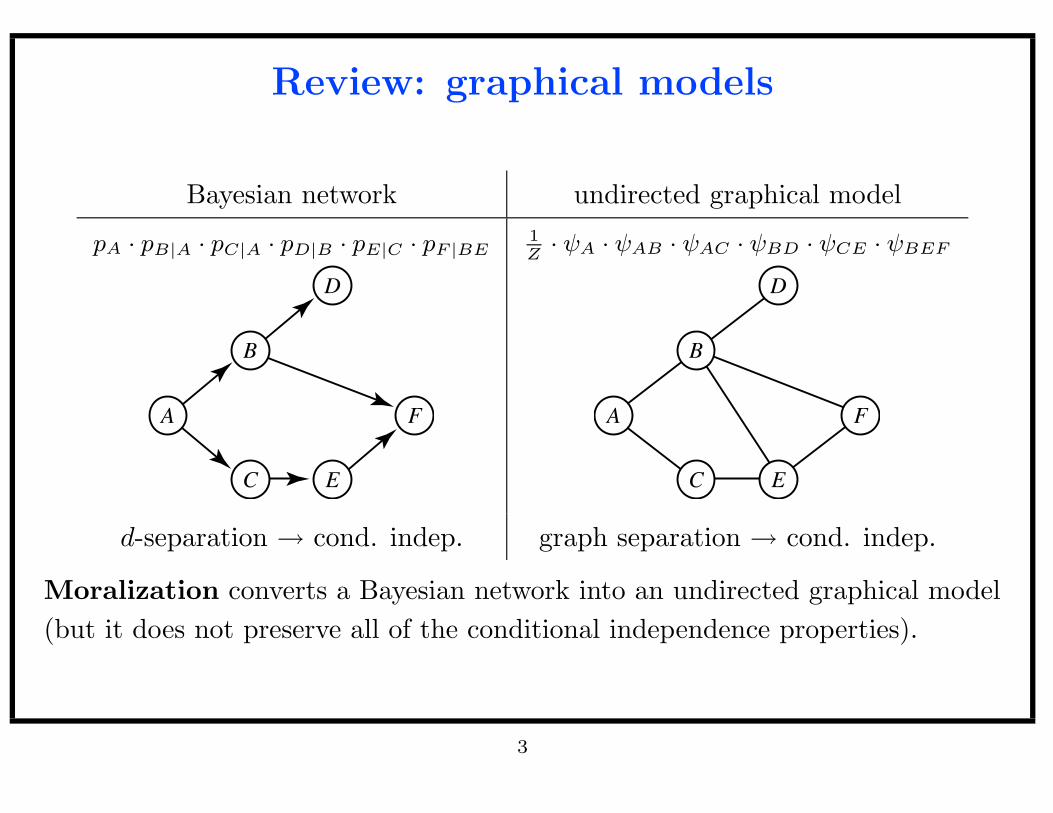
Review: graphical models
Bayesian network undirected graphical model
pA · pB|A · pC|A · pD|B · pE|C · pF |BE1
Z· ψA · ψAB · ψAC · ψBD · ψCE · ψBEF
A F
C
B
E
D
A F
C
B
E
D
d-separation → cond. indep. graph separation → cond. indep.
Moralization converts a Bayesian network into an undirected graphical model
(but it does not preserve all of the conditional independence properties).
3

A notation for sets of random variables
It is helpful when working with large, complex models to have a good notation
for sets of random variables.
• Let X = (Xi : i ∈ V ) be a vector random variable with density p.
• For each A ⊆ V , let XA4= (Xi : i ∈ A).
• For A,B ⊆ V , let pA4= pXA
and pA|B4= pXA|XB
.
Example. If V = {a, b, c} and A = {a, c} then
X =
Xa
Xb
Xc
and XA =
Xa
Xc
where Xa, Xb, and Xc are random variables.
4

A notation for assignments
We also need a notation for dealing flexibly with functions of many arguments.
• An assignment to A is a set of index-value pairs u = {(i, xi) : i ∈ A}, one
per index i ∈ A, where xi is in the range of Xi.
• Let XA be the set of assignments to XA (with X4= XV ).
• Building new assignments from given assignments:
– Given assignments u and v to disjoint subsets A and B, respectively,
their union u ∪ v is an assignment to A ∪B.
– If u is an assignment to A then the restriction of u to B ⊆ V is
uB4= {(i, xi) ∈ u : i ∈ B}, an assignment to A ∩B.
• If u = {(i, xi) : i ∈ A} is an assignment and f is a function, then
f(u)4= f(xi : i ∈ A)
5

Examples of the assignment notation
1. If p is the joint density of X then the marginal density of XA is
pA(v) =∑
u∈XA
p(v ∪ u), v ∈ XA
where A = V \A is the complement of A.
2. If p takes the form of a normalized product of potentials, we can write it as
p(u) =1
Z
∏
C∈C
ψC(uC), u ∈ X
where C is a set of subsets of V , and each ψC is a potential function that
depends only upon XC . The Markov graph of p has clique set C.
6

Review: the inference problem
• Input:
– a vector random variable X = (Xi : i ∈ V );
– a joint density for X of the form
p(u) =1
Z
∏
C∈C
ψC(uC)
– an evidence assignment w to E; and
– some query variables XQ.
• Output: pQ|E(·,w), the conditional density of XQ given the evidence w.
7
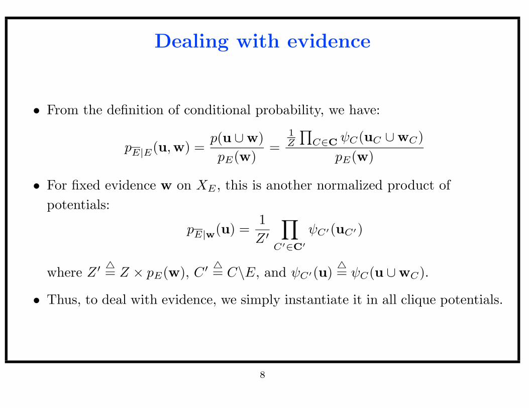
Dealing with evidence
• From the definition of conditional probability, we have:
pE|E(u,w) =p(u ∪ w)
pE(w)=
1Z
∏
C∈CψC(uC ∪ wC)
pE(w)
• For fixed evidence w on XE , this is another normalized product of
potentials:
pE|w(u) =1
Z ′
∏
C′∈C′
ψC′(uC′)
where Z ′ 4= Z × pE(w), C ′ 4
= C\E, and ψC′(u)4= ψC(u ∪ wC).
• Thus, to deal with evidence, we simply instantiate it in all clique potentials.
8

The reformulated inference problem
Given a joint density for X = (Xi : i ∈ V ) of the form
p(u) =1
Z
∏
C∈C
ψC(uC)
compute the marginal density of XQ:
pQ(v) =∑
u∈XQ
p(v ∪ u)
=∑
u∈XQ
1
Z
∏
C∈C
ψC(vC ∪ uC)
9

Review: Variable Elimination
• For each i ∈ Q, push in the sum over Xi and compute it:
pQ(v) =1
Z
∑
u∈XQ
∏
C∈C
ψC(vC ∪ uC)
=1
Z
∑
u∈XQ\{i}
∑
w∈X{i}
∏
C∈C
ψC(vC ∪ uC ∪ wC)
=1
Z
∑
u∈XQ\{i}
∏
C∈C
i 6∈C
ψC(vC ∪ uC)∑
w∈X{i}
∏
C∈C
i∈C
ψC(vC ∪ uC ∪ w)
=1
Z
∑
u∈XQ\{i}
∏
C∈C
i 6∈C
ψC(vC ∪ uC) · ψEi(vEi
∪ uEi)
This creates a new elimination clique Ei =⋃
C∈C
i∈CC\{i}.
• At the end we have pQ = 1ZψQ and we normalize to obtain pQ (and Z).
10
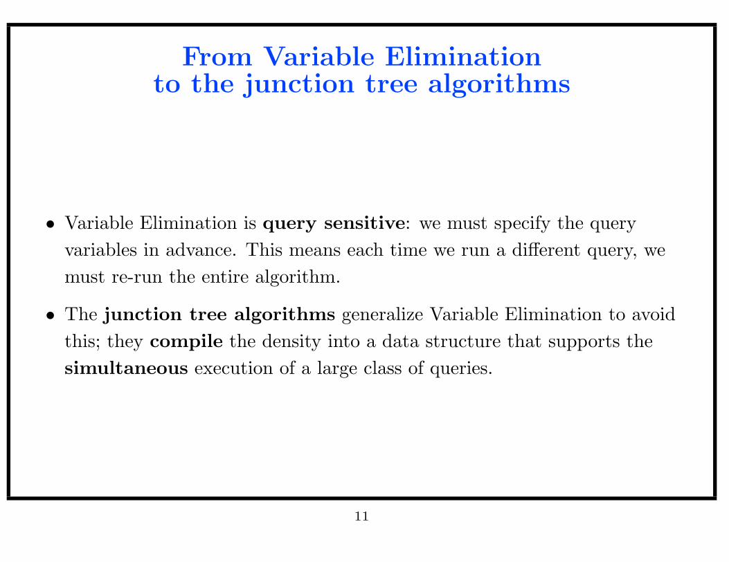
From Variable Eliminationto the junction tree algorithms
• Variable Elimination is query sensitive: we must specify the query
variables in advance. This means each time we run a different query, we
must re-run the entire algorithm.
• The junction tree algorithms generalize Variable Elimination to avoid
this; they compile the density into a data structure that supports the
simultaneous execution of a large class of queries.
11
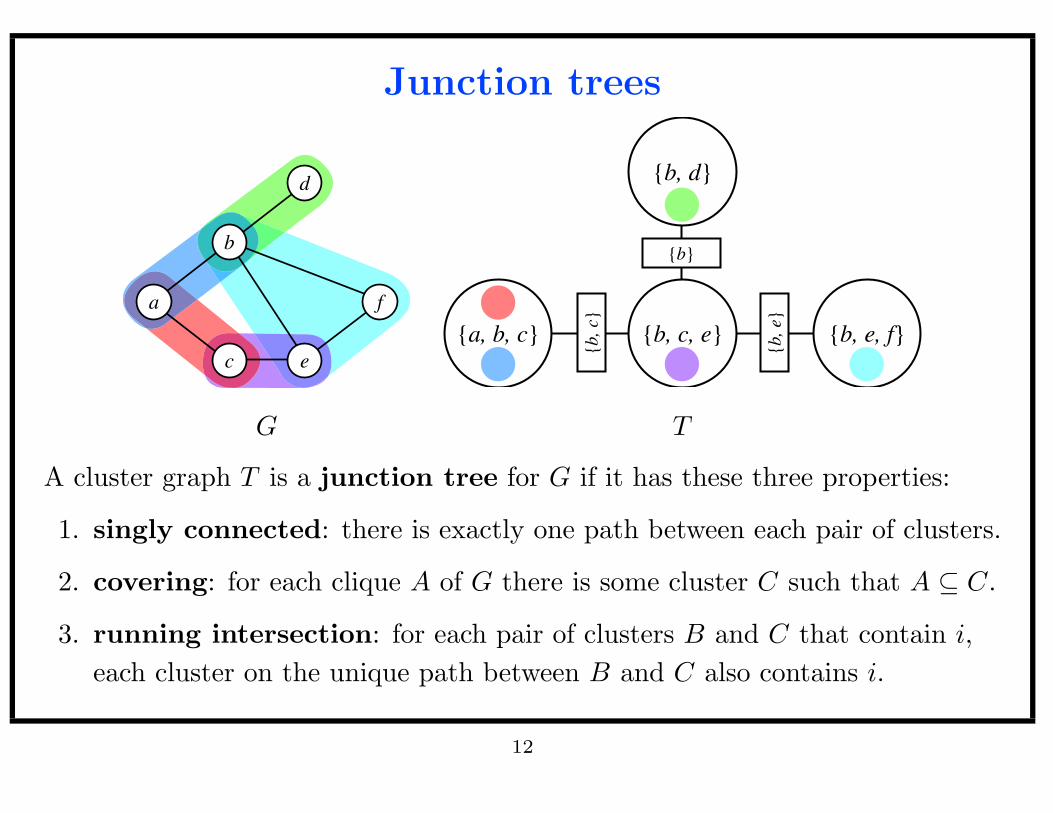
Junction trees
a f
c
b
e
d
{b, e, f}{b, c, e}
{b, d}
{a, b, c}
{b}
{b
, c}
{b
, e}
G T
A cluster graph T is a junction tree for G if it has these three properties:
1. singly connected: there is exactly one path between each pair of clusters.
2. covering: for each clique A of G there is some cluster C such that A ⊆ C.
3. running intersection: for each pair of clusters B and C that contain i,
each cluster on the unique path between B and C also contains i.
12
Building junction trees
• To build a junction tree:
1. Choose an ordering of the nodes and use Node Elimination to obtain a
set of elimination cliques.
2. Build a complete cluster graph over the maximal elimination cliques.
3. Weight each edge {B,C} by |B ∩ C| and compute a maximum-weight
spanning tree.
This spanning tree is a junction tree for G (see Cowell et al., 1999).
• Different junction trees are obtained with different elimination orders and
different maximum-weight spanning trees.
• Finding the junction tree with the smallest clusters is an NP-hard problem.
13

An example of building junction trees
1. Compute the elimination cliques (the order here is f, d, e, c, b, a).
a f
c
b
e
d
a
c
b
e
d
a
c
b
e
a
c
b
a
b
2. Form the complete cluster graph over the maximal elimination cliques and
find a maximum-weight spanning tree.
{b, e, f}
{b, c, e}
{b, d}
{a, b, c}
1
1
1
1
2
2
{b, e, f}{b, c, e}
{b, d}
{a, b, c}
{b}
{b
, c}
{b
, e}
14

Decomposable densities
• A factorized density
p(u) =1
Z
∏
C∈C
ψC(uC)
is decomposable if there is a junction tree with cluster set C.
• To convert a factorized density p to a decomposable density:
1. Build a junction tree T for the Markov graph of p.
2. Create a potential ψC for each cluster C of T and initialize it to unity.
3. Multiply each potential ψ of p into the cluster potential of one cluster
that covers its variables.
• Note: this is possible only because of the covering property.
15

The junction tree inference algorithms
The junction tree algorithms take as input a decomposable density and its
junction tree. They have the same distributed structure:
• Each cluster starts out knowing only its local potential and its neighbors.
• Each cluster sends one message (potential function) to each neighbor.
• By combining its local potential with the messages it receives, each cluster
is able to compute the marginal density of its variables.
16
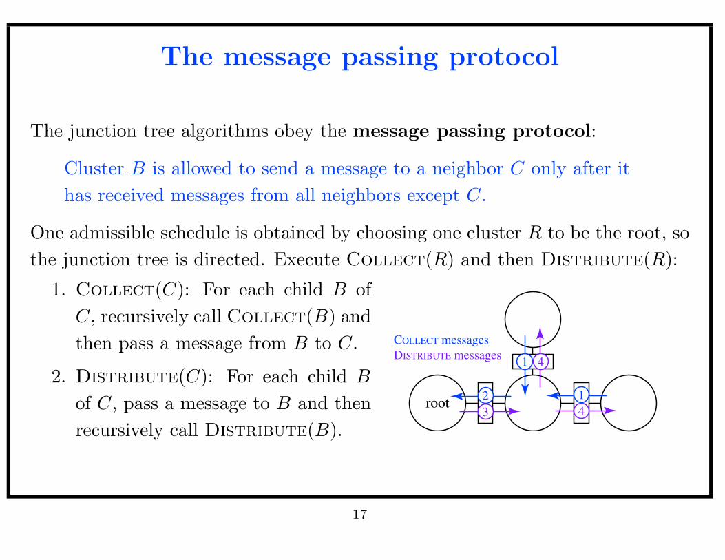
The message passing protocol
The junction tree algorithms obey the message passing protocol:
Cluster B is allowed to send a message to a neighbor C only after it
has received messages from all neighbors except C.
One admissible schedule is obtained by choosing one cluster R to be the root, so
the junction tree is directed. Execute Collect(R) and then Distribute(R):
1. Collect(C): For each child B of
C, recursively call Collect(B) and
then pass a message from B to C.
2. Distribute(C): For each child B
of C, pass a message to B and then
recursively call Distribute(B).
root
1
3 4
4
12
COLLECT messages
DISTRIBUTE messages
17

The Shafer–Shenoy Algorithm
• The message sent from B to C is defined as
µBC(u)4=
∑
v∈XB\C
ψB(u ∪ v)∏
(A,B)∈E
A 6=C
µAB(uA ∪ vA)
• Procedurally, cluster B computes the product of its local potential ψB and
the messages from all clusters except C, marginalizes out all variables
that are not in C, and then sends the result to C.
• Note: µBC is well-defined because the junction tree is singly connected.
• The cluster belief at C is defined as
βC(u)4= ψC(u)
∏
(B,C)∈E
µBC(uB)
This is the product of the cluster’s local potential and the messages
received from all of its neighbors. We will show that βC ∝ pC .
18

Correctness: Shafer–Shenoy is VariableElimination in all directions at once
• The cluster belief βC is computed by alternatingly multiplying cluster
potentials together and summing out variables.
• This computation is of the same basic form as Variable Elimination.
• To prove that βC ∝ pC , we must prove that no sum is “pushed in too far”.
• This follows directly from the running intersection property:
C
clusters containing i
i is summed out when
computing this message
messages with imessages without i
the running intersection property
guarantees the clusters containing i
constitute a connected subgraph
19

The hugin Algorithm
• Give each cluster C and each separator S a potential function over its
variables. Initialize:
φC(u) = ψC(u)
φS(u) = 1
• To pass a message from B to C over separator S, update
φ∗S(u) =∑
v∈XB\S
φB(u ∪ v)
φ∗C(u) = φC(u)φ∗S(uS)
φS(uS)
• After all messages have been passed, φC ∝ pC for all clusters C.
20
Correctness: hugin is a time-efficientversion of Shafer–Shenoy
• Each time the Shafer–Shenoy algorithm sends a message or computes its
cluster belief, it multiplies together messages.
• To avoid performing these multiplications repeatedly, the hugin algorithm
caches in φC the running product of ψC and the messages received so far.
• When B sends a message to C, it divides out the message C sent to B
from this running product.
21

Summary: the junction tree algorithms
Compile time:
1. Build the junction tree T :
(a) Obtain a set of maximal elimination cliques with Node Elimination.
(b) Build a weighted, complete cluster graph over these cliques.
(c) Choose T to be a maximum-weight spanning tree.
2. Make the density decomposable with respect to T .
Run time:
1. Instantiate evidence in the potentials of the density.
2. Pass messages according to the message passing protocol.
3. Normalize the cluster beliefs/potentials to obtain conditional densities.
22

Complexity of junction tree algorithms
• Junction tree algorithms represent, multiply, and marginalize potentials:
tabular Gaussian
storing ψC O(k|C|) O(|C|2)
computing ψB∪C = ψB × ψC O(k|B∪C|) O(|B ∪ C|2)
computing ψC\B(u) =∑
v∈XBψC(u ∪ v) O(k|C|) O(|B|
3|C|
2)
• The number of clusters in a junction tree and therefore the number of
messages computed is O(|V |).
• Thus, the time and space complexity is dominated by the size of the largest
cluster in the junction tree, or the width of the junction tree:
– In tabular densities, the complexity is exponential in the width.
– In Gaussian densities, the complexity is cubic in the width.
23

Generalized Distributive Law
• The general problem solved by the junction tree algorithms is the
sum-of-products problem: compute
pQ(v) ∝∑
u∈XQ
∏
C∈C
ψC(vC ∪ uC)
• The property used by the junction tree algorithms is the distributivity of ×
over +; more generally, we need a commutative semiring:
[0,∞) (+, 0) (×, 1) sum-product
[0,∞) (max, 0) (×, 1) max-product
(−∞,∞] (min,∞) (+, 0) min-sum
{T,F} (∨,F) (∧,T) Boolean
• Many other problems are of this form, including maximum a posteriori
inference, the Hadamard transform, and matrix chain multiplication.
24

Summary
• The junction tree algorithms generalize Variable Elimination to the
efficient, simultaneous execution of a large class of queries.
• The algorithms take the form of message passing on a graph called a
junction tree, whose nodes are clusters, or sets, of variables.
• Each cluster starts with one potential of the factorized density. By
combining this potential with the potentials it receives from its neighbors,
it can compute the marginal over its variables.
• Two junction tree algorithms are the Shafer–Shenoy algorithm and the
hugin algorithm, which avoids repeated multiplications.
• The complexity of the algorithms scales with the width of the junction tree.
• The algorithms can be generalized to solve other problems by using other
commutative semirings.
25