automatic design of decision-tree algorithms with ... design of decision-tree algorithms with...

Automatic Design of Decision-Tree Algorithmswith Evolutionary Algorithms

Rodrigo C. Barros [email protected] de Sao Paulo, Sao Carlos, Brazil

Marcio P. Basgalupp [email protected] Federal de Sao Paulo, Sao Jose dos Campos, Brazil

Andre C. P. L. F. de Carvalho [email protected] de Sao Paulo, Sao Carlos, Brazil

Alex A. Freitas [email protected] of Kent, Canterbury, United Kingdom

AbstractThis study reports the empirical analysis of a hyper-heuristic evolutionary algorithmthat is capable of automatically designing top-down decision-tree induction algo-rithms. Top-down decision-tree algorithms are of great importance, considering theirability of providing an intuitive and accurate knowledge representation for classifi-cation problems. The automatic design of these algorithms seems timely, given thelarge literature accumulated in more than 40 years of research in the manual designof decision-tree induction algorithms. The proposed hyper-heuristic evolutionary al-gorithm, HEAD-DT, is extensively tested using 20 public UCI data sets and 10 real-world microarray gene expression data sets. The algorithms automatically designedby HEAD-DT are compared with traditional decision-tree induction algorithms, suchas C4.5 and CART. Experimental results show that HEAD-DT is capable of generatingalgorithms which are significantly more accurate than C4.5 and CART.

KeywordsDecision trees, hyper-heuristics, automatic algorithm design, supervised machinelearning, data mining.

1 Introduction

Classification is a machine learning task that aims at building class prediction modelstaking into account a set of predictive attributes (also known as features). The outcomeof a classification model is the assigning of class labels to new instances whose onlyknown information are the values of the predictive attributes (i.e., whose class labels areunknown). The set of instances whose class labels is known is named the training set —{xi, yi}Ni=1 — where xi is the ith vector of predictive attributes xi = (xi1, x

i2, x

i3, ..., x

in)

and yi is the corresponding class label.A classification algorithm usually operates in two steps. In the first step, the train-

ing set {xi, yi}Ni=1 is used as input so that a classification model that represents therelationship between predictive attributes and class labels can be built. In the secondstep, the classification model is used to classify new instances whose class labels areunknown.

c©200X by the Massachusetts Institute of Technology Evolutionary Computation x(x): xxx-xxx

R.C. Barros, M.P. Basgalupp, A.C.P.L.F. de Carvalho, A.A. Freitas

Decision trees are one of the most employed classification methods to date. In fact,a relatively recent poll from the kdnuggets website1 pointed out decision trees as themost used classification method by researchers and practitioners, reaffirming its im-portance in machine learning classification tasks. They are an efficient nonparametricmethod whereby the input space is split into local regions in order to predict the classlabels (Alpaydin, 2010).

A decision tree can be seen as a graph G = (V,E) consisting of a finite, non-emptyset of nodes (vertices) V and a set of edges E. To be considered a decision tree, thisgraph must satisfy the following properties (Safavian and Landgrebe, 1991):

• The edges must be ordered pairs (v, w) of vertices, i.e., the graph must be directed;

• There can be no cycles within the graph, i.e., the graph must be acyclic;

• There is exactly one node, known as root, with no entering edges;

• Every node, except for the root, has exactly one entering edge;

• There is a unique path — a sequence of edges of the form(v1, v2), (v2, v3), ..., (vl−1, vl) — from the root to each node;

• When there is a path from node v to w, v 6= w, v is a proper ancestor of w and w isa proper descendant of v. A node with no proper descendant is called a leaf (or aterminal). All other nodes are called internal nodes (except for the root).

Root and internal nodes hold a test over a given predictive attribute (or a set ofpredictive attributes) from the data set. The edges correspond to the possible outcomesof the test, eventually leading to the leaf nodes, which are responsible for holding classlabels. For predicting the class label of a certain instance, one has to navigate throughthe decision tree. Starting from the root, one has to follow through the edges accordingto the results of the tests over the predictive attributes. When reaching a leaf node, theinformation it contains (class label) is usually assumed as the prediction outcome.

As it can be seen, decision trees are a natural alternative to powerful black-boxmethods, such as support vector machines (SVM) and neural networks (NNs), consid-ering their comprehensible nature that resembles the human reasoning. Decision-treeinduction algorithms present several advantages over other learning algorithms, suchas robustness to noise, low computational cost and ability to deal with redundant at-tributes (Tan et al., 2005). In Figure 1, an example of a general decision tree for classifi-cation is presented. Circles denote the root and internal nodes whilst boxes with roundcorners denote the leaf nodes.

There are exponentially many decision trees that can be grown from the same dataset. Induction of an optimal decision tree from a data set is considered to be a hardtask. For instance, Hyafil and Rivest (1976) have shown that constructing a minimalbinary tree with regard to the expected number of tests required for classifying an un-seen object is a NP-complete problem. Hancock et al. (1996) have proved that finding aminimal decision tree consistent with the training set is NP-Hard, which is also the caseof finding the minimal equivalent decision tree for a given decision tree (Zantema andBodlaender, 2000) and building the optimal decision tree from decision tables (Nau-mov, 1991). These studies indicate that growing optimal decision trees (a brute-forceapproach) is only feasible for very simple problems.

1http://www.kdnuggets.com/polls/2007/data_mining_methods.htm.

2 Evolutionary Computation Volume x, Number x

Automatic Design of Decision-Tree Algorithms with Evolutionary Algorithms

Figure 1: Example of a general decision tree for classification.

Hence, heuristics are necessary for dealing with the problem of growing decisiontrees. Several approaches developed in the last decades are capable of providing rea-sonably accurate — albeit suboptimal — decision trees in a reduced amount of time,such as bottom-up induction (Barros et al., 2011b), hybrid induction (Kim and Land-grebe, 1991), evolutionary induction (Basgalupp et al., 2009a,b; Barros et al., 2010, 2011c,2012b), and ensemble of trees (Breiman, 2001). Notwithstanding, no strategy has beenmore successful in generating accurate and comprehensible decision trees with lowcomputational effort than the greedy top-down induction strategy. Due to its popular-ity, a large number of approaches have been proposed for each one of the design compo-nents of top-down decision-tree induction algorithms. For instance, new measures fornode splitting tailored to a vast number of application domains have been proposed,as well as many different strategies for selecting multiple attributes for composing thenode rule. There are also studies in the literature that survey the numerous approachesfor pruning a decision tree (Breslow and Aha, 1997; Esposito et al., 1997). It is clear thatby improving these design components, we can obtain more robust top-down decision-tree induction algorithms.

Bearing in mind that the manual improvement of decision-tree design compo-nents has been carried out for the past 40 years, we believe that automatically design-ing decision-tree induction algorithms could provide a faster, less-tedious — and atleast equally effective — strategy for improving decision-tree induction algorithms inthe years to come. This belief is partly supported by a proof of concept that evo-lutionary algorithms can effectively design new data mining algorithms competitivewith conventional ones, as reported in (Pappa and Freitas, 2010). In that work, agrammar-based genetic programming system was investigated to automatically designa rule induction algorithm, which is another type of classification algorithm, and theautomatically-designed algorithms were shown to be competitive with state-of-the-artmanually-designed rule induction algorithms.

Evolutionary Computation Volume x, Number x 3


In order to automatically design decision-tree induction algorithms, we proposea hyper-heuristic evolutionary algorithm, named HEAD-DT. We first envisioned theproblem of automatically designing decision-tree induction algorithms in (Barros et al.,2011a). In this new study, we investigate the effectiveness of automatically designingdecision-tree induction algorithms in both benchmarking and bioinformatics data. Thispaper is an extended version of a previous conference paper (Barros et al., 2012a), pro-viding a more detailed description of the proposed approach and also presenting newcomputational results and their analysis for 10 real-world bioinformatics (gene expres-sion) data sets.

This paper is organized as follows. Section 2 offers a background on decision treesfor readers unfamiliar with the topic. Section 3 presents in detail the HEAD-DT al-gorithm. Sections 4 and 5 describe the experimental methodology and the obtainedresults, respectively, whereas Section 6 discusses relevant aspects regarding the effec-tiveness and efficiency of HEAD-DT. Section 7 presents related work and Section 8concludes the paper with our final thoughts and future work suggestions.

2 Background on Decision Trees

Automatically generating classification rules in the form of decision trees has been ob-ject of study of most research fields in which data exploration techniques have beendeveloped (Murthy, 1998). Disciplines such as engineering (pattern recognition), statis-tics, decision theory, and more recently artificial intelligence (machine learning), havea large number of studies dedicated to the generation and application of decision trees.In statistics, we can trace the origins of decision trees to works that proposed buildingbinary segmentation trees for understanding the relationship between predictors anddependent variable. Some examples are AID (Sonquist et al., 1971) and CHAID (Kass,1980). Decision-tree induction algorithms, and induction methods in general, arosein machine learning to avoid the knowledge acquisition bottleneck in expert systems(Murthy, 1998).

Specifically regarding top-down induction of decision trees (by far the most popu-lar approach of decision-tree induction), Hunt’s Concept Learning System (CLS) (Huntet al., 1966) can be regarded as the pioneering work for inducing decision trees. Sys-tems that directly descend from Hunt’s CLS are ID3 (Quinlan, 1986), ACLS (Pattersonand Niblett, 1983) and Assistant (Kononenko et al., 1984).

At a high level of abstraction, Hunt’s algorithm can be recursively defined inonly two steps. Let Xt be the set of training instances associated with node t andy = {y1, y2, ..., yk} be the class labels in a k-class problem (Tan et al., 2005):

1. if all instances in Xt belong to the same class yi then t is a leaf node labeled as yi;

2. if Xt contains instances that belong to more than one class, an attribute test con-dition is selected to partition the instances into subsets. A child node is createdfor each outcome of the test and the instances in Xt are distributed to the childrenbased on the outcomes. Recursively apply the algorithm to each child.

Hunt’s simplified algorithm is the basis for most current top-down decision-treeinduction algorithms. Nevertheless, its assumptions are too stringent for practical use.For instance, it would only work if every combination of attribute values is present inthe training data, and if the training data is inconsistency-free (each combination has aunique class label).

Hunt’s algorithm was improved in many ways. Its stopping criterion, for exam-ple, as expressed in step 1, requires all leaf nodes to be pure (i.e., belonging to the same



class). In most practical cases, this constraint leads to very large decision trees, whichtend to suffer from overfitting. Possible solutions to overcome this problem are pre-maturely stopping the tree growth when a minimum level of impurity is reached, orperforming a pruning step after the tree has been fully grown. Another design issue ishow to select the attribute test condition to partition the instances into smaller subsets.In Hunt’s original approach, a cost-driven function was responsible for partitioningthe tree. Subsequent algorithms, such as ID3 (Quinlan, 1986) and C4.5 (Quinlan, 1993),make use of information theory based functions for partitioning nodes in purer subsets.

These improvements were achieved by human investigation of several design al-ternatives. We believe that evolutionary algorithms (EA) are capable to evolve newefficient decision-tree induction algorithms by automatically finding a good combina-tion of different heuristics, many of them present in known induction algorithms. In thenext section, we present an EA designed to evolve the design components of decision-tree induction algorithms, HEAD-DT.

3 HEAD-DT

HEAD-DT is a hyper-heuristic algorithm able to automatically design top-downdecision-tree induction algorithms. Hyper-heuristics can automatically generate newheuristics suited to a given problem or class of problems. This is accomplished by com-bining, through an evolutionary algorithm, components or building-blocks of humandesigned heuristics (Burke et al., 2009).

HEAD-DT is a regular generational EA in which individuals are collections ofbuilding blocks (heuristics) from decision-tree induction algorithms. In Figure 2, wepresent its evolutionary scheme.

Initial

PopulationEvaluation

Tournament

Selection

New Population

Complete?Stop?

Best

IndividualTest

META-TRAINING

SET

META-TEST

SET

NoYes

Yes

No

Reproduction Crossover Mutation

pr pc pm

Figure 2: HEAD-DT evolutionary scheme.

Each individual in HEAD-DT is encoded as an integer string (see Figure 3), andeach gene has a different range of supported values. We divided the genes into fourcategories that represent the major building blocks (design components) of a decision-tree induction algorithm: (i) split genes; (ii) stopping criteria genes; (iii) missing valuesgenes; and (iv) pruning genes. We detail each category next.

3.1 Split Genes

These genes are concerned with the task of selecting the predictive attribute to splitthe data in the current node of the decision tree. A decision rule based on the selectedattribute is thus generated, and the input data is filtered according to the outcomes of



Figure 3: Linear genome for evolving decision-tree induction algorithms.

this rule, and the process continues recursively. HEAD-DT uses two genes to modelthe split component of a decision-tree algorithm: split criterion and split type.

3.1.1 Split Criterion GeneThe first gene, split criterion, is an integer that indexes one of the 15 splitting crite-ria implemented: information gain (Quinlan, 1986), Gini index (Breiman et al., 1984),global mutual information (Gleser and Collen, 1972), G statistics (Mingers, 1987),Mantaras criterion (De Mantaras, 1991), hypergeometric distribution (Martin, 1997),Chandra-Varghese criterion (Chandra and Varghese, 2009), DCSM (Chandra et al.,2010), χ2 (Mingers, 1989), mean posterior improvement (Taylor and Silverman, 1993),normalized gain (Jun et al., 1997), orthogonal criterion (Fayyad and Irani, 1992), twoing(Breiman et al., 1984), CAIR (Ching et al., 1995) and gain ratio (Quinlan, 1993).

The most well-known univariate criteria are based on Shannon’s entropy (Shan-non, 1948). Entropy is known to be a unique function that satisfies the four axioms ofuncertainty. It represents the average amount of information when coding each classinto a codeword with ideal length according to its probability. The first splitting cri-terion based on entropy was the global mutual information (GMI) (Gleser and Collen,1972). Afterwards, the well-known information gain (Quinlan, 1986) became a standardafter appearing in algorithms like ID3 (Quinlan, 1986) and Assistant (Kononenko et al.,1984). It belongs to the class of the so-called impurity-based criteria. Quinlan (Quin-lan, 1986) acknowledged the fact that the information gain is biased towards attributeswith many values. To deal with this problem, he proposed the gain ratio (Quinlan,1993), which basically normalizes the information gain by the entropy of the attributebeing tested. Several variations of the gain ratio were proposed, e.g., the normalizedgain (Jun et al., 1997). Alternatives to entropy-based criteria are the class of distance-based measures, i.e., criteria, which evaluate separability, divergency or discriminationbetween classes. Examples are the Gini index (Breiman et al., 1984), the twoing crite-rion (Breiman et al., 1984), the orthogonality criterion (Fayyad and Irani, 1992), amongothers. We also included lesser-known criteria, such as CAIR (Ching et al., 1995) andmean posterior improvement (Taylor and Silverman, 1993), as well as the more recentChandra-Varghese (Chandra and Varghese, 2009) and DCSCM (Chandra et al., 2010),to enhance the diversity of options for generating splits in a decision tree.

3.1.2 Split Type GeneThe second gene, split type, is a binary gene that indicates whether the splits of a de-cision tree are going to be necessarily binary or perhaps multi-way. In a binary tree,every split has only two outcomes, which means that nominal attributes with manycategories will be divided into two subsets, each representing an aggregation over sev-eral categories. In a multi-way tree, nominal attributes are divided according to theirnumber of categories, i.e., one edge (outcome) for each category. In both cases, numeric



attributes always partition the tree into two subsets, (≤ threshold and > threshold).

3.2 Stopping Criteria Genes

The second category of genes is related to the stopping criteria component of decision-tree induction algorithms. The top-down induction of a decision tree is recursive and itcontinues until a stopping criterion (also known as pre-pruning) is satisfied. HEAD-DTuses two genes to model the stopping criteria component of decision trees: criterion andparameter.

3.2.1 Stopping Criterion GeneThe first gene, stopping criterion, selects among the five following different strategiesfor stopping the tree growth:

• Reaching class homogeneity: when all instances that reach a given node belong tothe same class, there is no reason to split this node any further. This criterion canbe combined with any of the following criteria;

• Reaching the maximum tree depth: a parameter tree depth can be specified to avoiddeep trees. Range: [2, 10] levels;

• Reaching the minimum number of instances for a non-terminal node: a parameterminimum number of instances for a non-terminal node can be specified to avoid (orat least alleviate) the data fragmentation problem in decision trees. Range: [1, 20]instances;

• Reaching the minimum percentage of instances for a non-terminal node: same asabove, but instead of the actual number of instances, we set the minimum percent-age of instances. The parameter is thus relative to the total number of instances ina data set. Range: [1%, 10%] the total number of instances;

• Reaching a predictive accuracy threshold within a node: a parameter accuracyreached can be specified for halting the growth of the tree when the predictive ac-curacy within a node (majority of instances) has reached a given threshold. Range:{70%, 75%, 80%, 85%, 90%, 95%, 99%}.

3.2.2 Stopping Parameter GeneThe second gene, stopping parameter, dynamically adjusts a value in the range [0, 100]to the corresponding strategy. For instance, if the strategy selected by gene stoppingcriterion is reaching a predictive accuracy threshold within a node, the following mappingfunction is executed:

param = ((value mod 7)× 5) + 70 (1)

This function maps from [0, 100] to {70, 75, 80, 85, 90, 95, 100}, which is almost whatwas defined as the range of strategy reaching a predictive accuracy threshold. The final stepsubtracts 1 from the resulting parameter value if it is equal to 100. Similar mappingfunctions are executed dynamically to adjust the ranges of gene stopping parameter.

3.3 Missing Values Genes

Handling missing values is an important task in decision-tree induction. Missing val-ues can harm the tree induction process and also its use for the classification of newexamples. During the tree induction, there are two moments in which we need to deal



with missing values: splitting criterion evaluation and instances distribution. To dealwith these scenarios, HEAD-DT uses three genes to model the missing values compo-nent of decision trees: mv split, mv distribution, and mv classification.

3.3.1 mv Split GeneDuring the split criterion evaluation for a node t based on an attribute ai, we imple-mented the following strategies: (i) ignore all instances whose value of ai is missing(Friedman, 1977; Breiman et al., 1984); (ii) imputation of missing values with either themode (nominal attributes) or the mean/median (numeric attributes) of all instances int (Clark and Niblett, 1989); (iii) weight the splitting criterion value (calculated in node twith regard to ai) by the proportion of missing values (Quinlan, 1989); and (iv) imputa-tion of missing values with either the mode (nominal attributes) or the mean/median(numeric attributes) of all instances in twhose class attribute is the same of the instancewhose ai value is being imputed (Loh and Shih, 1997).

3.3.2 mv Distribution GeneFor deciding to which child node a training instance xj should go to, considering a splitfor node t over ai, we adopted the following options: (i) ignore instance xj (Quinlan,1986); (ii) treat instance xj as if it has the most common value of ai (mode or mean),regardless of its class (Quinlan, 1989); (iii) treat instance xj as if it has the most commonvalue of ai (mode or mean) considering the instances that belong to the same class asxj ; (iv) assign instance xj to all partitions (Friedman, 1977); (v) assign instance xj to thepartition with the largest number of instances (Quinlan, 1989); (vi) weight instance xjaccording to the partition probability (Quinlan, 1993; Kononenko et al., 1984); and (vii)assign instance xj to the most probable partition, considering the class of xj (Loh andShih, 1997).

3.3.3 mv Classification GeneFor classifying an unseen test instance xj , considering a split in node t over ai, we usedthe strategies: (i) explore all branches of t combining the results (Quinlan, 1987a); (ii)take the route to the most probable partition (largest subset); (iii) halt the classificationprocess and assign the instance xj to the majority class of node t (Quinlan, 1989).

3.4 Pruning Genes

Pruning is usually performed in decision trees to enhance tree comprehensibility byreducing its size while maintaining (or even improving) its predictive accuracy. It wasoriginally conceived as a strategy for tolerating noisy data, though it was found toimprove decision tree predictive accuracy in many noisy data sets (Breiman et al., 1984;Quinlan, 1986, 1987b). We designed two genes in HEAD-DT for pruning: method andparameter.

3.4.1 Pruning Method GeneThe first gene, pruning method, indexes one of the following five approaches for prun-ing a decision tree (and also the option of not pruning at all):

• Reduced-error pruning (REP) is a conceptually simple strategy proposed by Quin-lan (Quinlan, 1987b). It uses a pruning set (part of the training set) to evaluatethe goodness of a given subtree from T . The idea is to evaluate each non-terminalnode t regarding the classification error in the pruning set. If this error decreaseswhen we replace the subtree T (t) rooted on t by a leaf node, then T (t) must be



pruned. Quinlan also imposes a constraint: a node t cannot be pruned if it containsa subtree that yields a lower classification error in the pruning set. The practicalconsequence of this constraint is that REP should be performed in a bottom-upfashion. The REP pruned tree T ′ presents an interesting optimality property: itis the smallest most accurate tree resulting from pruning original tree T (Quinlan,1987b). Besides this optimality property, another advantage of REP is its linearcomplexity, since each node is visited only once in T . An obvious disadvantageis the need of a pruning set, which means one has to divide the original trainingset, resulting in less instances to grow the tree. This disadvantage is particularlyserious for small data sets.

• Also proposed by Quinlan (1987b), the pessimistic error pruning (PEP) uses thetraining set for both growing and pruning the tree. The apparent error rate, i.e.,the error rate calculated for the training set, is optimistically biased and cannotbe used to decide whether pruning should be performed or not. Quinlan proposesadjusting the apparent error according to the continuity correction for the binomialdistribution in order to provide a more realistic error rate. PEP is computed in atop-down fashion, and if a given node t is pruned, its descendants are not exam-ined, which makes this pruning strategy very computationally efficient. However,Esposito et al. (Esposito et al., 1997) point out that the introduction of the continu-ity correction in the estimation of the error rate has no theoretical justification, sinceit was never applied to correct over-optimistic estimates of error rates in statistics.

• Originally proposed in (Niblett and Bratko, 1986) and further extended in (Cestnikand Bratko, 1991), minimum error pruning (MEP) is a bottom-up approach thatseeks to minimize the expected error rate for unseen cases. It uses an ad-hoc param-eter m for controlling the level of pruning. Usually, the higher the value of m, themore severe the pruning. Cestnik and Bratko (Cestnik and Bratko, 1991) suggestthat a domain expert should set m according to the level of noise in the data. Al-ternatively, a set of trees pruned with different values of m could be offered to thedomain expert, so he/she can choose the best one according to his/her experience.

• Cost-complexity pruning (CCP) is the post-pruning strategy of the CART system,detailed in (Breiman et al., 1984). It has two steps: (i) generate a sequence of in-creasingly smaller trees, beginning with T and finishing with the root node of T , bysuccessively pruning the subtree yielding the lowest cost complexity, in a bottom-up fashion; (ii) choose the best tree among the sequence based on its relative sizeand predictive accuracy (either on a pruning set, or provided by a cross-validationprocedure in the training set). The idea behind step 1 is that the pruned tree Ti+1

is obtained by pruning the subtrees that show the lowest increase in the apparenterror (error in the training set) per pruned leaf. Regarding step 2, CCP chooses thesmallest tree whose error (either on the pruning set or on cross-validation) is nothigher than one standard error (SE) larger than the lowest error observed in thesequence of trees.

• Finally, error-based pruning (EBP), proposed by Quinlan and implemented as thedefault pruning strategy of C4.5 (Quinlan, 1993), is an improvement over PEP. Itis based on a far more pessimistic estimate of the expected error. Unlike PEP, EBPperforms a bottom-up search, and it carries out not only the replacement of non-terminal nodes by leaves but also grafting of subtree T (t) onto the place of parent



INDIVIDUAL

DECISION-TREE

ALGORITHMDTTRAINING VALIDATION STATS

FITNESS EVALUATION

META-TRAINING SET

70% 30%

DATA SET90%

10%

META-TEST SET

Figure 4: Fitness evaluation from one data set in the meta-training set.

t. For deciding whether to replace a non-terminal node by a leaf (subtree replace-ment), to graft a subtree onto the place of its parent (subtree raising) or not to pruneat all, a pessimistic estimate of the expected error is calculated by using an upperconfidence bound. An advantage of EBP is the new grafting operation that allowspruning useless branches without ignoring interesting lower branches. A draw-back of the method is the presence of an ad-hoc parameter, CF . Smaller values ofCF result in more pruning.

3.4.2 Pruning Parameter GeneThe second gene, pruning parameter, is in the range [0, 100] and its value is dynami-cally mapped by a function, according to the pruning method selected (similar to thestopping parameter gene). For REP, the parameter is the percentage of training datato be used in the pruning set (varying within the interval [10%, 50%]). For PEP, the pa-rameter is the number of standard errors (SEs) to adjust the apparent error, in the set{0.5, 1, 1.5, 2}. For MEP, the parameter m may range within [0, 100]. For CCP, there aretwo parameters: the number of SEs (in the same range than PEP) and the pruning setsize (in the same range as REP). Finally, for EBP, the parameter CF may vary withinthe interval [1%, 50%].

3.5 Fitness Evaluation

During the fitness evaluation, HEAD-DT employs a meta-training set for assessing thequality of each individual throughout evolution. It also employes a meta-test set, whichis used to assess the quality of the evolved decision-tree induction algorithm (the bestindividual in Figure 2). There are two distinct approaches for dealing with the meta-training and meta-test sets:

1. Evolving a decision-tree induction algorithm tailored to one specific data set.

2. Evolving a decision-tree induction algorithm from multiple data sets.

In the first case (see Figure 4), we have a specific data set for which we want todesign a decision-tree induction algorithm. The meta-training set is thus comprisedof the training data we have available for the data set at hand, and the meta-test setis comprised of the test data (belonging to the same data set) we have available forevaluating the performance of the algorithm.



INDIVIDUAL

DECISION-TREE

ALGORITHMTRAINING 2

DT 1

DT 2

DT n

TRAINING 1

TRAINING n

VALIDATION 1

VALIDATION 2

VALIDATION n

STATS 1

STATS 2

STATS n

... ... ... ...

FITNESS EVALUATION

META-TRAINING SET

Figure 5: Fitness evaluation from multiple data sets in the meta-training set.

In the second case (see Figure 5), we have multiple data sets comprising the meta-training set, and possibly multiple (but different) data sets comprising the meta-test set.This strategy can be employed with two different objectives: (i) designing a decision-tree induction algorithm that performs reasonably well in a wide variety of data sets(i.e., data sets with very different structural characteristics and/or from very distinctapplication domains, e.g. finance, medicine, bioinformatics, etc); and (ii) designing adecision-tree induction algorithm that is tailored to a particular application domain orto a specific statistical profile. In both cases, the main goal is to generate inductionalgorithms tailored to a set of data sets, which may be from the same domain or not.

In this paper, we focus on the first fitness approach — generating one decision-treeinduction algorithm per data set. The second approach is a topic left for future research.As fitness function, we investigate both predictive accuracy and F-Measure (harmonicmean of precision and recall) (Tan et al., 2005). These performance measures can bedefined in terms of four variables: true positives (tp), true negatives (tn), false positives(fp), and false negatives (fn). True positives (negatives) is the number of instancesthat were correctly predicted as belonging to the “positive” (“negative”) class, whereasfalse positives (negatives) is the number of instances that were incorrectly predicted asbelonging to the “positive” (“negative”) class. With these four variables, we can defineaccuracy, precision, recall, and F-Measure, respectively, as:

accuracy =tp+ tn

tp+ tn+ fp+ fn(2)

precision =tp

tp+ fp(3)

recall =tp

tp+ fn(4)

FMeasure = 2× precision× recallprecision+ recall

(5)

Note that this formulation assumes that the classification problem at hand is bi-nary, i.e., comprised of two classes: positive and negative. Nevertheless, it can be triv-ially extended to account for multi-class problems. For instance, one can compute themeasure for each class — assuming each class to be the “positive” class in turn — and(weight-)average the per-class measures. A discussion about the pros and cons of ac-curacy and F-measure as predictive performance measures will be presented later.



3.6 Evolutionary Cycle

The evolution of individuals in HEAD-DT follows the scheme presented in Figure 2.The 9-gene linear genome of an individual in HEAD-DT is comprised of the build-ing blocks described in the earlier sections: [split criterion, split type, stopping criterion,stopping parameter, pruning strategy, pruning parameter, mv split, mv distribution, mv classi-fication], where mv stands for missing value.

The first step of HEAD-DT is the generation of the initial population, in which apopulation of n individuals is randomly generated (random number generation withinthe genes acceptable range of values). The individuals from the current populationparticipate in a pairwise tournament selection procedure for defining those that willundergo genetic operators. Individuals may participate in either uniform crossover,random uniform gene mutation, or reproduction, the three mutually-exclusive geneticoperators employed in HEAD-DT. In addition, HEAD-DT employs an elitism strategy,in which the best i% individuals are kept from one generation to the next.

One possible individual encoded by the 9-gene linear string representation is[4, 1, 2, 77, 3, 91, 2, 5, 1], which accounts for Algorithm 1.

Algorithm 1 — Example of an algorithm automatically designed by HEAD-DT.1) Recursively split nodes with the G statistics criterion;2) Create one edge for each category in a nominal split;3) Perform step 1 until class-homogeneity or the maximum tree depth of 7 levels

(77 mod 9) + 2) is reached;4) Perform MEP pruning with m = 91;5) When dealing with missing values:

5.1) Impute missing values with mode/mean during split calculation;5.2) Distribute missing-valued instances to the partition with the largest number of

instances;5.3) For classifying an instance with missing values, explore all branches and

combine the results.

4 Experimental Methodology

4.1 Data sets

To assess the relative performance of the algorithms automatically designed by HEAD-DT, we employ well-known UCI public data sets (Frank and Asuncion, 2010). In ad-dition, we test the effectiveness of the automatically-generated algorithms tailored toeach of 10 real-world gene expression data sets (de Souto et al., 2008). The 30 datasets used for testing the effectiveness of HEAD-DT are summarized in Table 1, wherethe fifth and sixth columns describe the number of numerical and nominal attributes,respectively. The other column names are self-explanatory.

4.2 Baseline Algorithms and Statistical Analysis

We compare the resulting decision-tree induction algorithms with the most well-knownand widely-used decision-tree induction algorithms to date: C4.5 (Quinlan, 1993) andCART (Breiman et al., 1984). Since HEAD-DT is a non-deterministic method, its resultsare averaged over 5 different runs (varying the random seed in each run).

In order to provide some reassurance about the validity and non-randomness ofthe obtained results, we present the results of statistical tests by following the approachproposed by Demsar (Demsar, 2006). In brief, this approach seeks to compare multiplealgorithms on multiple data sets, and it is based on the use of the Friedman test witha corresponding post-hoc test. The Friedman test is a non-parametric counterpart of



Table 1: Summary of the 30 data sets used in the experiments.source data set # instances # attributes # numeric # nominal % missing # classes

UCI

abalone 4177 8 7 1 0.00 30anneal 898 38 6 32 0.00 6arrhythmia 452 279 206 73 0.32 16audiology 226 69 0 69 2.03 24bridges version1 107 12 3 9 5.53 6car 1728 6 0 6 0.00 4cylinder bands 540 39 18 21 4.74 2glass 214 9 9 0 0.00 7hepatitis 155 19 6 13 5.67 2iris 150 4 4 0 0.00 3kdd synthetic 600 61 60 1 0.00 6segment 2310 19 19 0 0.00 7semeion 1593 265 265 0 0.00 2shuttle landing 15 6 0 6 28.89 2sick 3772 30 6 22 5.54 2tempdiag 120 7 1 6 0.00 2tep.fea 3572 7 7 0 0.00 3vowel 990 13 10 3 0.00 11winequality red 1599 11 11 0 0.00 10winequality white 4898 11 11 0 0.00 10

Gene

alizadeh-2000-v1 42 1095 1095 0 0.0 2

Expression

armstrong-2002-v1 72 1081 1081 0 0.0 2armstrong-2002-v2 72 2194 2194 0 0.0 3bittner-2000 38 2201 2201 0 0.0 2liang-2005 37 1411 1411 0 0.0 3ramaswamy-2001 190 1363 1363 0 0.0 14risinger-2003 42 1771 1771 0 0.0 4tomlins-2006 104 2315 2315 0 0.0 5tomlins-2006-v2 92 1288 1288 0 0.0 4yeoh-2002-v1 248 2526 2526 0 0.0 2

the well-known ANOVA, as follows. Let Rji be the rank of the jth of k algorithms onthe ith of N data sets. The Friedman test compares the average ranks of algorithms,Rj =

1N

∑iR

ji . The Friedman statistic, given by:

χ2F =

12N

k(k + 1)

∑j

R2j −

k(k + 1)2

4

(6)

is distributed according to χ2F with k − 1 degrees of freedom, when N and k are large

enough.Iman and Davenport (Iman and Davenport, 1980) showed that Friedman’s χ2

F isundesirably conservative and derived an adjusted statistic:

Ff =(N − 1)× χ2

F

N × (k − 1)− χ2F

(7)

which is distributed according to the F -distribution with k − 1 and (k − 1)(N − 1)degrees of freedom.

If the null hypothesis of similar performances is rejected, we proceed with theNemenyi post-hoc test for pairwise comparisons. The performance of two classifiers issignificantly different if their corresponding average ranks differ by at least the criticaldifference

CD = qα

√k(k + 1)

6N(8)



where critical values qα are based on the Studentized range statistic divided by√2.

4.3 Parameters

The baseline algorithms CART (Breiman et al., 1984) and C4.5 (Quinlan, 1993) wereused with the default parameter values proposed by their authors, which typically rep-resent robust values that work well across different data sets. None of the algorithms,including HEAD-DT, had their parameter values optimized to individual data sets,since the goal is to evaluate a parameter settings’ generalization ability across a widerange of data sets, as usual in the supervised machine learning literature.

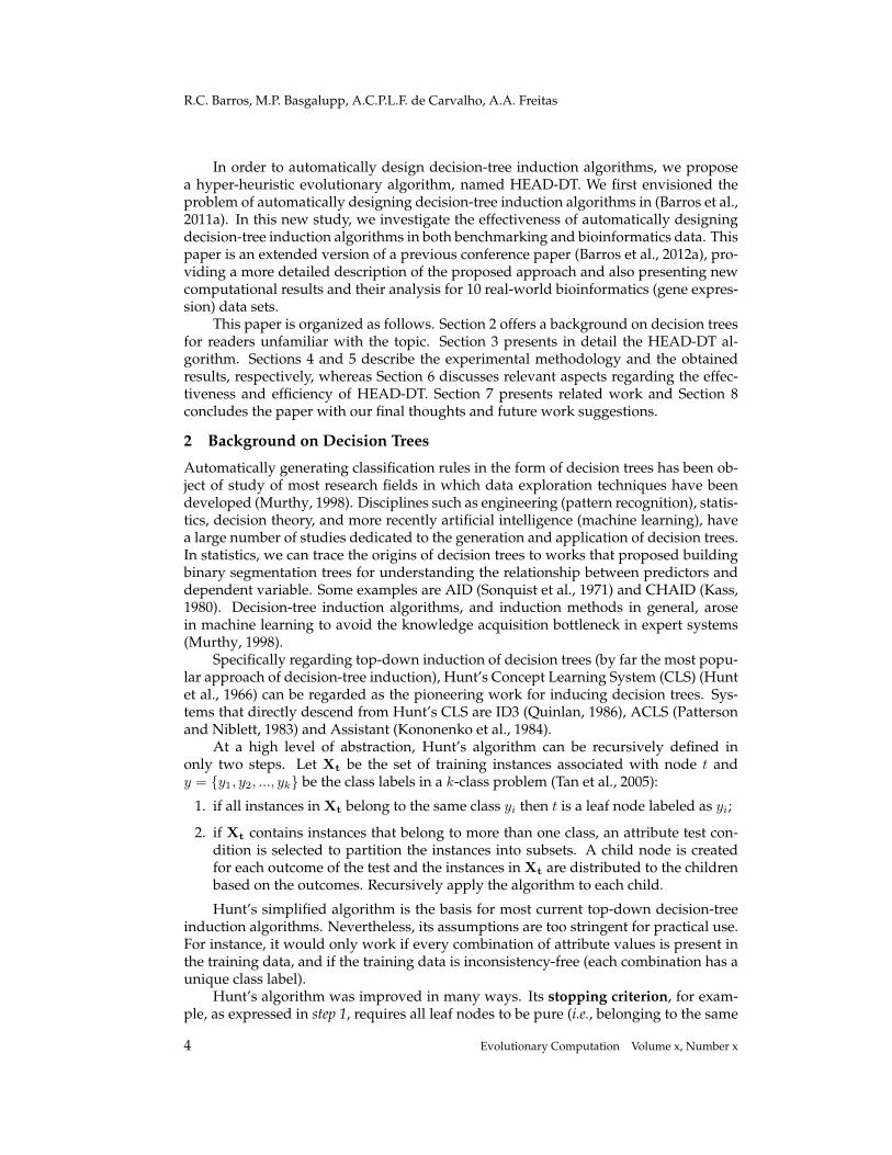
HEAD-DT was configured with the following parameter values described in Ta-ble 2. These values were defined in previous non-exhaustive empirical tests, and nofurther attempt of optimizing these values was made. A more robust parameter opti-mization procedure is left for future research.

Table 2: Parameter values for HEAD-DT.Parameter Description Value

Number of Individuals 100Number of Generations 100Tournament Selection Size 2Elitism Rate 5%Crossover Rate 90%Mutation Rate 5%Reproduction Rate 5%

5 Results

In this section, we present the results obtained by HEAD-DT with the strategy of gen-erating one algorithm per data set. Recall that, in this case, both the meta-training andmeta-test sets contain data from a specific data set. We used 10-fold cross-validation toevaluate the results provided by HEAD-DT and by the baseline algorithms C4.5 (Quin-lan, 1993) and CART (Breiman et al., 1984).

For the UCI data sets, we employed predictive accuracy (see Equation (2)) as fit-ness function, whereas for the gene expression (GE) data sets we employed the F-Measure (see Equation (5)), considering that most GE data sets are quite imbalanced.The results for the UCI datasets were also reported in our previous work (Barros et al.,2012a), but the results for the GE datasets are a new contribution of this paper.

5.1 Results for the UCI Data Sets

Table 3 shows the classification accuracy of CART, C4.5, and HEAD-DT for the 20 UCIdata sets. It illustrates the average accuracy over the 10-fold cross-validation runs ±the standard deviation of the accuracy obtained in these runs (best absolute values inbold). It is possible to see that HEAD-DT generates more accurate trees in 13 out of the20 data sets. CART provides more accurate trees in two data sets, and C4.5 in none. Inthe remaining 5 data sets, no method was superior to the others.

To evaluate the statistical significance of the predictive accuracy results, we calcu-lated the average rank for CART, C4.5 and HEAD-DT: 2.375, 2.2, and 1.425, respectively.The average ranks suggest that HEAD-DT is the best performing method regarding ac-curacy. The calculation of Friedman’s χ2

F is given by:



Table 3: Classification accuracy of CART, C4.5 and HEAD-DT — UCI data sets.CART C4.5 HEAD-DT

abalone 0.26± 0.02 0.22± 0.02 0.20± 0.02anneal 0.98± 0.01 0.99± 0.01 0.99± 0.01arrhythmia 0.71± 0.05 0.65± 0.04 0.65± 0.04audiology 0.74± 0.05 0.78± 0.07 0.80± 0.06bridges version1 0.41± 0.07 0.57± 0.10 0.60± 0.12car 0.97± 0.02 0.93± 0.02 0.98± 0.01cylinder bands 0.60± 0.05 0.58± 0.01 0.72± 0.04glass 0.70± 0.11 0.69± 0.04 0.73± 0.10hepatitis 0.79± 0.05 0.79± 0.06 0.81± 0.08iris 0.93± 0.05 0.94± 0.07 0.95± 0.04kdd synthetic 0.88± 0.00 0.91± 0.04 0.97± 0.03segment 0.96± 0.01 0.97± 0.01 0.97± 0.01semeion 0.94± 0.01 0.95± 0.02 1.00± 0.00shuttle landing 0.95± 0.16 0.95± 0.16 0.95± 0.15sick 0.99± 0.01 0.99± 0.00 0.99± 0.00tempdiag 1.00± 0.00 1.00± 0.00 1.00± 0.00tep.fea 0.65± 0.02 0.65± 0.02 0.65± 0.02vowel 0.82± 0.04 0.83± 0.03 0.89± 0.04winequality red 0.63± 0.02 0.61± 0.03 0.64± 0.03winequality white 0.58± 0.02 0.61± 0.03 0.63± 0.03

χ2F =

12× 20

3× 4

[2.3752 + 2.22 + 1.4252 − 3× 42

4

]= 10.225 (9)

and the Iman’s F statistic is given by:

Ff =(20− 1)× 10.225

20× (3− 1)− 10.22= 6.52 (10)

The critical value of F (k − 1, (k − 1)(n − 1)) = F (2, 38) for α = 0.05 is 3.25. SinceFf > F0.05(2, 38) (6.52 > 3.25), the null-hypothesis is rejected. We proceed with apost-hoc Nemenyi test to find which method provides the best accuracy. The criticaldifference CD is given by:

CD = 2.343×√

3× 4

6× 20= 0.74 (11)

The difference between the average rank of HEAD-DT and C4.5 is 0.775, while thedifference between HEAD-DT and CART is 0.95. Since both the differences are largerthanCD, the performance of HEAD-DT is significantly better than both C4.5 and CARTregarding predictive accuracy.

Table 4 shows the classification F-Measure of CART, C4.5, and HEAD-DT for thesame UCI data sets. It can be seen that HEAD-DT generates better trees (regardless ofthe class imbalance problem) in 16 out of the 20 data sets. CART generates the best treein two data sets, while C4.5 does not induce the best tree for any data set.

We calculated the average rank for CART, C4.5, and HEAD-DT: 2.5, 2.225 and1.275, respectively. The average rank suggest that HEAD-DT is the best performingmethod regarding the F-Measure. The calculation of Friedman’s χ2

F is given by:

χ2F =

12× 20

3× 4

[2.52 + 2.2252 + 1.2752 − 3× 42

4

]= 16.525 (12)




Table 4: Classification F-Measure of CART, C4.5 and HEAD-DT — UCI data sets.CART C4.5 HEAD-DT


Ff =(20− 1)× 16.525

20× (3− 1)− 16.525= 13.375 (13)

Since Ff > F0.05(2, 38) (13.375 > 3.25), the null-hypothesis is rejected. The dif-ference between the average rank of HEAD-DT and C4.5 is 0.95, while the differencebetween HEAD-DT and CART is 1.225. Since both the differences are larger than CD(0.74), the performance of HEAD-DT is significantly better than both C4.5 and CARTregarding the F-Measure.

Table 5 shows the size of decision trees (measured as the number of tree nodes)generated by C4.5, CART and HEAD-DT. It can be seen that CART generates smallertrees in 15 out of the 20 data sets. C4.5 generates smaller trees in 2 data sets, and HEAD-DT in only one data set. The statistical analysis is given below:

χ2F =

12× 20

3× 4

[1.22 + 22 + 2.82 − 3× 42

4

]= 25.6 (14)

Ff =(20− 1)× 33.78

20× (3− 1)− 25.6= 33.78 (15)

Since Ff > F0.05(2, 38) (33.78 > 3.25), the null-hypothesis is rejected. The differ-ence between the average rank of HEAD-DT and C4.5 is 0.8, while the difference be-tween HEAD-DT and CART is 1.6. Since both the differences are larger than CD (0.74),HEAD-DT generates trees which are significantly larger than both C4.5 and CART forthese UCI data sets.

5.2 Results for the Gene Expression Data Sets

In this section, we present the results for 10 microarray gene expression (GE) data sets(de Souto et al., 2008). Microarray technology enables expression level measurementfor thousands of genes in parallel, given a biological tissue. Once combined, a fixednumber of microarray experiments are comprised in a gene expression data set. Theconsidered data sets are related to different types or subtypes of cancer (e.g., prostate,lung and skin) and comprehend the two flavors in which the technology is generally



Table 5: Tree size of CART, C4.5 and HEAD-DT trees — UCI data sets.CART C4.5 HEAD-DT


available: single channel and double channel. The classification task consists of classi-fying different instances according to their gene (attribute) expression levels. Note thatthe classification of microarray data is challenging because the number of instancesis much smaller than the number of attributes, which makes classification algorithmsapplied to such data prone to overfitting.

Table 6 shows the classification accuracy of CART, C4.5, and HEAD-DT regardingthe 10 GE data sets. It illustrates the average accuracy over the 10-fold cross-validationruns ± the standard deviation of the accuracy obtained in these runs (best absolutevalues in bold). One can see that HEAD-DT generates more accurate trees in 9 out ofthe 10 data sets. In the remaining data set (yeoh-2002-v1), all methods provide the samedecision tree (and thus, obtain the same accuracy value).

Table 6: Classification accuracy of CART, C4.5 and HEAD-DT — GE data sets.data set CART C4.5 HEAD-DT

alizadeh-2000-v1 0.71± 0.16 0.68± 0.20 0.76± 0.18armstrong-2002-v1 0.90± 0.07 0.89± 0.06 0.91± 0.11armstrong-2002-v2 0.85± 0.05 0.83± 0.05 0.90± 0.10bittner-2000 0.53± 0.18 0.49± 0.16 0.56± 0.19liang-2005 0.71± 0.14 0.76± 0.19 0.79± 0.17ramaswamy-2001 0.60± 0.09 0.61± 0.05 0.63± 0.08risinger-2003 0.52± 0.15 0.53± 0.19 0.60± 0.29tomlins-2006-v1 0.58± 0.20 0.58± 0.18 0.58± 0.17tomlins-2006-v2 0.59± 0.15 0.58± 0.17 0.61± 0.09yeoh-2002-v1 0.99± 0.02 0.99± 0.02 0.99± 0.02

We calculated the average rank for CART, C4.5, and HEAD-DT: 2.25, 2.65, and 1.1,respectively. The average rank suggest that HEAD-DT is the best performing methodregarding accuracy. The calculation of Friedman’s χ2

F is given by:

χ2F =

12× 10

3× 4

[2.652 + 2.252 + 1.12 − 3× 42

4

]= 12.95 (16)




Ff =(10− 1)× 12.95

10× (3− 1)− 12.95= 16.53 (17)

F (k − 1, (k − 1)(n − 1)) = F (2, 18) for α = 0.05 is 3.55. Since Ff > F0.05(2, 18)(16.53 > 3.55), the null-hypothesis is rejected. We proceed with the post-hoc pairwiseNemenyi test. The critical difference CD is given by:

CD = 2.343×√

3× 4

6× 10= 1.05 (18)

The difference between the average rank of HEAD-DT and C4.5 is 1.55, while thedifference between HEAD-DT and CART is 1.15. Since both differences are larger thanCD (1.05), the performance of HEAD-DT is significantly better than both C4.5 andCART regarding the predictive accuracy in the GE data sets.

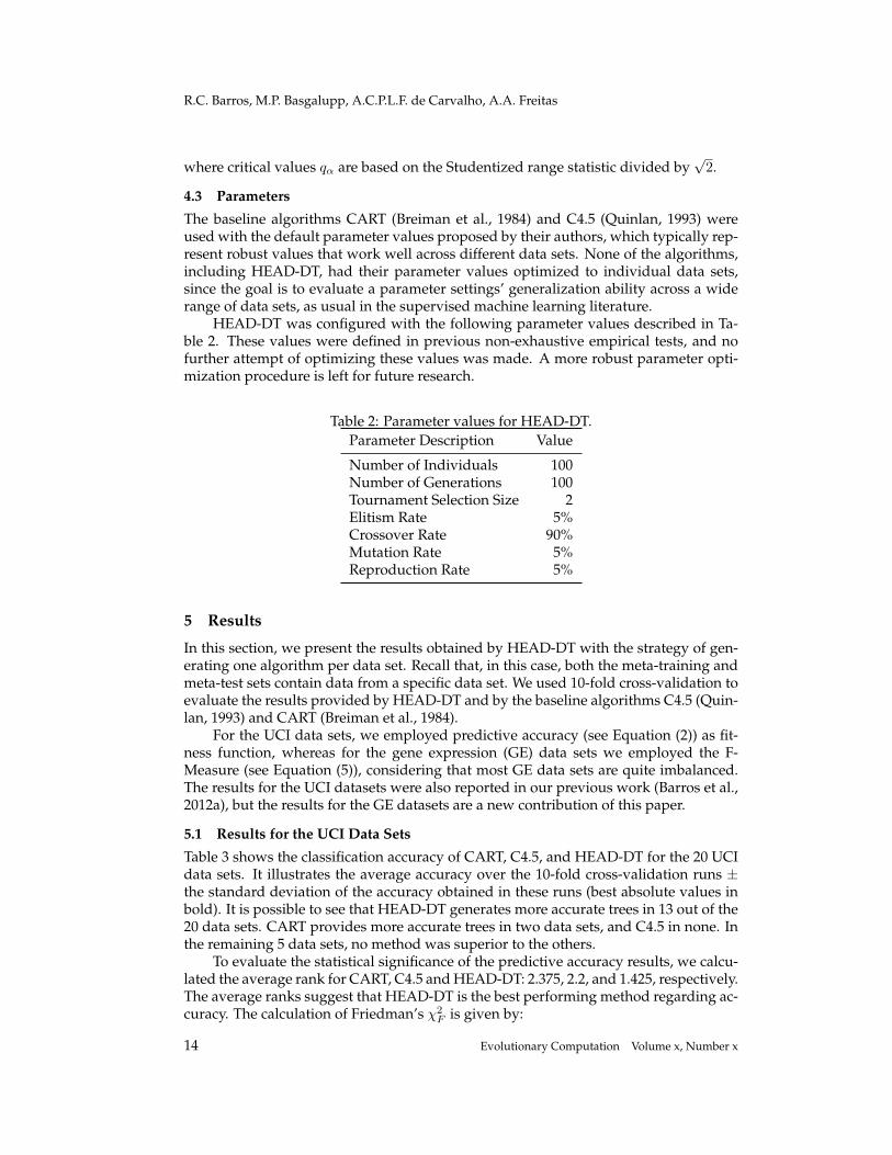
Next, Table 7 shows the classification F-Measure of CART, C4.5, and HEAD-DT forthe same GE data sets. The experimental results show that HEAD-DT generates bettertrees (regardless of the class imbalance problem) in 8 out of the 10 data sets. CART andC4.5 generate the best tree for tomlins2006-v1, while all methods generate the same treefor yeah-2002-v1.

Table 7: Classification F-Measure of CART, C4.5 and HEAD-DT — GE data sets.data set CART C4.5 HEAD-DT


We calculated the average rank for CART, C4.5, and HEAD-DT: 2.2, 2.75, and 1.05,respectively. The average rank suggest that HEAD-DT is the best performing methodregarding the F-Measure. The calculation of Friedman’s χ2

F is given by:

χ2F =

12× 10

3× 4

[2.752 + 2.22 + 1.052 − 3× 42

4

]= 15.05 (19)


Ff =(10− 1)× 15.05

10× (3− 1)− 15.05= 27.36 (20)

Since Ff > F0.05(2, 18) (27.36 > 3.55), the null-hypothesis is rejected. The dif-ference between the average rank of HEAD-DT and C4.5 is 1.7, while the differencebetween HEAD-DT and CART is 1.15. Since both the differences are larger than CD(1.05), the performance of HEAD-DT is significantly better than both C4.5 and CARTregarding the F-Measure.

Finally, Table 8 presents the average tree size for CART, C4.5, and HEAD-DT re-garding the GE data sets. CART provides the smaller trees for all data sets (it generatesthe same tree than C4.5 in data set yeah-2002-v1).



Table 8: Tree size of CART, C4.5 and HEAD-DT trees — GE data sets.data set CART C4.5 HEAD-DT


We calculated the average rank for CART, C4.5, and HEAD-DT: 1.3, 2.4, and 2.3,respectively. The average rank suggests that CART generates smaller trees than bothC4.5 and HEAD-DT. The calculation of Friedman’s χ2

F is given by:

χ2F =

12× 10

3× 4

[2.42 + 2.32 + 1.32 − 3× 42

4

]= 7.40 (21)


Ff =(10− 1)× 7.40

10× (3− 1)− 7.40= 5.29 (22)

Since Ff > F0.05(2, 18) (5.29 > 3.55), the null-hypothesis is rejected. The differencebetween the average rank of HEAD-DT and C4.5 is 0.1, while the difference betweenHEAD-DT and CART is 1.0. The size of trees generated by CART are significantlysmaller than those generated by C4.5 and HEAD-DT. There are no significant differ-ences between HEAD-DT and C4.5 regarding the tree size, though.

5.3 Summary

In the experiments performed for this study, the decision-tree induction algorithmsautomatically designed by HEAD-DT induced decision trees with better predictiveperformance than both CART and C4.5, which are very popular and very effectivemanually-designed decision-tree induction algorithms. In both experiments (with UCIand GE data sets), HEAD-DT consistently presented better results with statistical as-surance. The performance evaluation measures we employed in these experiments —accuracy and F-Measure — are among the most well-known and used measures in datamining and machine learning classification problems.

Regarding tree complexity, which was measured as the total number of nodes ina tree (tree size), we observed that CART usually induced much smaller trees, proba-bly due to its particular pruning method (cost complexity pruning). Nevertheless, wesaw that smaller trees do not necessarily translate into better performance, since thetrees generated by the automatically-designed algorithms are significantly more accu-rate than those generated by CART.

We conclude from these experiments that HEAD-DT is indeed an effective alter-native to state-of-the-art decision-tree induction algorithms C4.5 and CART. Next, webroaden our discussion by commenting on other issues involved in decision-tree in-duction, and also on the trade-off between HEAD-DT’s predictive performance andcomputational efficiency.



6 Discussion

In this section, we discuss three important topics to support the empirical analysispresented in the previous section: (i) the accuracy dilemma and when preferring F-Measure for evaluating decision-tree induction algorithms; (ii) the empirical (and theo-retic) time complexity of HEAD-DT, and also of the decision-tree induction algorithmsit generates; and (iii) an example of decision-tree induction algorithm automaticallydesigned by HEAD-DT.

6.1 Accuracy vs F-Measure

The fact that HEAD-DT designs algorithms that induce significantly more accurate de-cision trees than C4.5 and CART is very encouraging. Notwithstanding, we must pointout that accuracy may be a misleading performance measure. For instance, suppose wehave a data set whose class distribution is very skewed: 90% of the instances belong toclass A and 10% to class B. An algorithm that always classifies instances as belongingto class A would achieve 90% of accuracy, even though it never predicts a class-B in-stance. In this case, assuming that class B is equally important (or even more so) thanclass A, we would prefer an algorithm with lower accuracy, but which could eventuallycorrectly predict some instances as belonging to the rare class B.

The previous example illustrates the importance of not relying only on accuracywhen designing an algorithm. F-Measure is the harmonic mean of precision and recall,and thus rewards solutions that present a good trade-off between these two measures.Hence, for imbalanced-class problems, F-Measure should be preferred over accuracy.

In the experimental analysis performed in the previous section, recall that we opti-mized solutions towards accuracy (in the UCI data sets) and F-Measure (in the GE datasets) by varying HEAD-DT fitness function. We observed that, regardless of the mea-sure being optimized, HEAD-DT was able to generate robust solutions for balancedand imbalanced data sets.

6.2 HEAD-DT Complexity Analysis

Regarding execution time, it is clear that HEAD-DT is slower than either C4.5 andCART. Considering that there are 100 individuals executed for 100 generations, there isa maximum (worst case) of 10000 fitness evaluations of decision trees.

We recorded the execution time of both breeding operations and fitness evaluation(one thread was used for breeding and another for evaluation). The total time of breed-ing is absolutely negligible (a few milliseconds in a full evolutionary cycle), regardlessof the data set being used (breeding does not consider any domain-specific informa-tion). Indeed, breeding individuals in the form of an integer string is known to be quiteefficient in the EA research field.

Fitness evaluation, on the other hand, is the bottleneck of HEAD-DT. In the largestUCI data set (winequality white), HEAD-DT took 2.5 hours to be fully executed (oneiteration of the cross-validation procedure, in a full evolutionary cycle of 100 genera-tions). In the smallest UCI data set (shuttle landing), HEAD-DT took only 0.72 secondsto be fully executed, which means the fitness evaluation time can largely vary accord-ing to the data set size.

It should be noted that, even in cases where a run of HEAD-DT took several hours,this is still a very short time in the context of algorithm design, since, in general, evena machine learning researcher with expertise in decision-tree induction would takemuch longer to design a novel decision-tree algorithm that is competitive with C4.5and CART.



The computational complexity of algorithms like C4.5 and CART is O(m×n log n)(m is the number of attributes and n the number of instances), plus a term regardingthe specific pruning method. Considering that breeding takes negligible time, we cansay that in the worst case scenario, HEAD-DT time complexity is O(i×g×m×n log n),where i is the number of individuals and g is the number of generations. In practice,the number of evaluations is much smaller than i × g, due to the fact that repeatedindividuals are not re-evaluated. In addition, individuals selected by elitism and by re-production (instead of crossover) are also not re-evaluated, saving computational time.

6.3 Example of an Evolved Decision-Tree Algorithm

For illustrating a novel decision-tree induction algorithm designed by HEAD-DT, letus consider the semeion data set, in which HEAD-DT managed to achieve maximumaccuracy and F-Measure (which was not the case for CART and C4.5). The algorithmdesigned by HEAD-DT is presented in Algorithm 2. It is indeed novel, since no algo-rithm in the literature combines components such as the Chandra-Varghese criterionwith MEP pruning. Furthermore, it chooses MEP as its pruning method, which is asurprise considering that MEP is usually a neglected pruning method in the decisiontree literature.

The main advantage of HEAD-DT is that it automatically searches for the suitablecomponents (with their own biases) according to the data set being investigated. It ishard to believe that a human researcher would combine such a distinct set of compo-nents like those in Algorithm 2 to achieve 100% accuracy in a particular data set.

Algorithm 2 — decision-tree induction algorithm designed by HEAD-DT for the se-meion data set.1) Recursively split nodes using the Chandra-Varghese criterion;2) Aggregate nominal splits in binary subsets;3) Perform step 1 until class-homogeneity or the minimum number of 5 instances is reached;4) Perform MEP pruning with m = 10;5) When dealing with missing values:

5.1) Calculate the split of missing values by performing unsupervised imputation;5.2) Distribute missing values by assigning the instance to all partitions;5.3) For classifying an instance, explore all branches and combine the results.

7 Related Work

To the best of our knowledge, no work to date has attempted to automatically designfull decision-tree induction algorithms (except of course our previous work (Barroset al., 2012a) which has been extended in this paper, as mentioned in the Introduction).The most related approach to this work is HHDT (Hyper-Heuristic Decision Tree) (Vellaet al., 2009). It proposes an EA for evolving heuristic rules in order to determine the bestsplitting criterion to be used in non-terminal nodes. Whilst this approach is a first stepto automate the design of decision-tree induction algorithms, it evolves a single com-ponent of the algorithm (the choice of splitting criterion), and thus should be furtherextended for being able to generate full decision-tree induction algorithms.

A somewhat related approach is the one presented by Delibasic et al. (Delibasicet al., 2011). The authors propose a framework for combining decision-tree compo-nents, and test 80 different combination of design components on 15 benchmark datasets. This approach is not a hyper-heuristic, since it does not present a heuristic tochoose among different heuristics. It simply selects a fixed number of component com-binations and test them all against traditional decision-tree induction algorithms (C4.5,



CART, ID3 and CHAID). We believe that our strategy is more robust, since by using anevolutionary algorithm, it can search for solutions in a much larger search space. Cur-rently, HEAD-DT searches in the space of more than 127 million different candidatedecision-tree induction algorithms.

8 Conclusions and Future Work

In this paper, we presented HEAD-DT, a hyper-heuristic evolutionary algorithmthat automatically designs top-down decision-tree induction algorithms. Top-downdecision-tree induction algorithms have been manually improved in 40 years of re-search, leading to a large number of proposed approaches for each of their design com-ponents. Since the human manual combination of all available design components ofthese algorithms would be unfeasible, we believe the evolutionary search of HEAD-DT constitutes a robust and efficient solution for the design of new and effective algo-rithms.

We performed a thorough experimental analysis in which the algorithms automat-ically designed by HEAD-DT were compared to the state-of-the-art decision-tree induc-tion algorithms CART (Breiman et al., 1984) and C4.5 (Quinlan, 1993). In this analysis,we evaluated the effectiveness of HEAD-DT in two scenarios: (i) general performancein 20 well-known UCI data sets with very different characteristics, from very differ-ent application domains; (ii) domain-specific performance in 10 real-world microarraygene expression data sets. We assessed the performance of HEAD-DT through two dis-tinct performance evaluation measures (predictive accuracy and F-Measure), and a treecomplexity measure (tree size). In both scenarios, the experimental results suggestedthat HEAD-DT can generate decision-tree induction algorithms with predictive perfor-mance significantly higher than CART and C4.5, though sometimes generating largertrees. Bearing in mind that an accurate prediction system is widely preferred over asignificantly less accurate (but simpler) system, we believe that HEAD-DT arises as arobust algorithm for future applications of decision trees.

As future work, we intend to develop a multi-objective fitness function, consider-ing the trade-off between predictive performance and parsimony. In addition, we planto investigate whether a more sophisticated search system, such as grammar-basedgenetic programming, can outperform our current HEAD-DT implementation. Opti-mizing the evolutionary parameters of HEAD-DT is also a topic left for future research.

Acknowledgements

The authors would like to thank Coordenacao de Aperfeicoamento de Pessoal de NıvelSuperior (CAPES), Conselho Nacional de Desenvolvimento Cientıfico e Tecnologico(CNPq) and Fundacao de Amparo a Pesquisa do Estado de Sao Paulo (FAPESP) forfunding this research.

ReferencesAlpaydin, E. (2010). Introduction to Machine Learning. The MIT Press, 2nd edition.

Barros, R., Basgalupp, M., Ruiz, D., Carvalho, A., and Freitas, A. (2010). Evolutionary modeltree induction. In Proceedings of the ACM Symposium on Applied Computing (SAC 2010), pages1131–1137.

Barros, R. C., Basgalupp, M. P., de Carvalho, A. C., and Freitas, A. A. (2011a). Towards the auto-matic design of decision tree induction algorithms. In Proceedings of the 13th Annual ConferenceCompanion on Genetic and Evolutionary computation, GECCO ’11, pages 567–574, New York, NY,USA. ACM.



Barros, R. C., Basgalupp, M. P., de Carvalho, A. C., and Freitas, A. A. (2012a). A Hyper-Heuristic Evolutionary Algorithm for Automatically Designing Decision-Tree Algorithms. InProceedings of the 14th International Conference on Genetic and Evolutionary Computation Confer-ence, GECCO ’12, pages 1237–1244, New York, NY, USA. ACM.

Barros, R. C., Basgalupp, M. P., de Carvalho, A. C. P. L. F., and Freitas, A. A. (2012b). A Survey ofEvolutionary Algorithms for Decision-Tree Induction. IEEE Transactions on Systems, Man andCybernetics - Part C: Applications and Reviews, 42(3):291–312.

Barros, R. C., Cerri, R., Jaskowiak, P. A., and de Carvalho, A. C. P. L. F. (2011b). A Bottom-UpOblique Decision Tree Induction Algorithm. In Proceedings of the 11th International Conferenceon Intelligent Systems Design and Applications, pages 450 –456.

Barros, R. C., Ruiz, D. D., and Basgalupp, M. P. (2011c). Evolutionary model trees for handlingcontinuous classes in machine learning. Information Sciences, 181:954–971.

Basgalupp, M., Barros, R. C., de Carvalho, A., Freitas, A., and Ruiz, D. (2009a). Legal-tree: alexicographic multi-objective genetic algorithm for decision tree induction. In Proceedings ofthe ACM Symposium on Applied Computing (SAC 2009), pages 1085–1090, Hawaii, USA.

Basgalupp, M. P., de Carvalho, A. C. P. L. F., Barros, R. C., Ruiz, D. D., and Freitas, A. A. (2009b).Lexicographic multi-objective evolutionary induction of decision trees. International Journal ofBioinspired Computation, 1(1/2):105–117.

Breiman, L. (2001). Random forests. Machine Learning, 45(1):5–32.

Breiman, L., Friedman, J. H., Olshen, R. A., and Stone, C. J. (1984). Classification and RegressionTrees. Wadsworth.

Breslow, L. and Aha, D. (1997). Simplifying decision trees: A survey. The Knowledge EngineeringReview, 12(01):1–40.

Burke, E. K., Hyde, M. R., Kendall, G., Ochoa, G., Ozcan, E., and Woodward, J. R. (2009). Explor-ing Hyper-heuristic Methodologies with Genetic Programming. In Colaborative ComputationalIntelligence, pages 177–201. Springer.

Cestnik, B. and Bratko, I. (1991). On estimating probabilities in tree pruning. In Proceedings of theEuropean working session on learning on Machine learning (EWSL’91), pages 138–150. Springer.

Chandra, B., Kothari, R., and Paul, P. (2010). A new node splitting measure for decision treeconstruction. Pattern Recognition, 43(8):2725–2731.

Chandra, B. and Varghese, P. P. (2009). Moving towards efficient decision tree construction. In-formation Sciences, 179(8):1059–1069.

Ching, J., Wong, A., and Chan, K. (1995). Class-dependent discretization for inductive learningfrom continuous and mixed-mode data. IEEE Transactions on Pattern Analysis and MachineIntelligence, 17(7):641–651.

Clark, P. and Niblett, T. (1989). The CN2 induction algorithm. Machine Learning, 3(4):261–283.

De Mantaras, R. L. (1991). A Distance-Based Attribute Selection Measure for Decision Tree In-duction. Machine Learning, 6(1):81–92.

de Souto, M., Costa, I., de Araujo, D., Ludermir, T., and Schliep, A. (2008). Clustering cancer geneexpression data: a comparative study. BMC Bioinformatics, 9(1):497.

Delibasic, B., Jovanovic, M., Vukicevic, M., Suknovic, M., and Obradovic, Z. (2011). Component-based decision trees for classification. Intelligent Data Analysis, 15:1–38.

Demsar, J. (2006). Statistical Comparisons of Classifiers over Multiple Data Sets. Journal of Ma-chine Learning Research, 7:1–30.



Esposito, F., Malerba, D., and Semeraro, G. (1997). A Comparative Analysis of Methods for Prun-ing Decision Trees. IEEE Transactions on Pattern Analysis and Machine Intelligence, 19(5):476–491.

Fayyad, U. and Irani, K. (1992). The attribute selection problem in decision tree generation. InNational Conference on Artificial Intelligence, pages 104–110.

Frank, A. and Asuncion, A. (2010). UCI machine learning repository. available at http://archive.ics.uci.edu/ml.

Friedman, J. H. (1977). A recursive partitioning decision rule for nonparametric classification.IEEE Transactions on Computers, 100(4):404–408.

Gleser, M. and Collen, M. (1972). Towards automated medical decisions. Computers and BiomedicalResearch, 5(2):180–189.

Hancock, T., Jiang, T., Li, M., and Tromp, J. (1996). Lower bounds on learning decision lists andtrees. Information and Computation, 126(2).

Hunt, E. B., Marin, J., and Stone, P. J. (1966). Experiments in induction. Academic Press, New York,NY, USA.

Hyafil, L. and Rivest, R. (1976). Constructing optimal binary decision trees is np-complete. Infor-mation Processing Letters, 5(1):15–17.

Iman, R. and Davenport, J. (1980). Approximations of the critical region of the friedman statistic.Communications in Statistics, pages 571–595.

Jun, B., Kim, C., Song, Y.-Y., and Kim, J. (1997). A New Criterion in Selection and Discretizationof Attributes for the Generation of Decision Trees. IEEE Transactions on Pattern Analysis andMachine Intelligence, 19(2):1371–1375.

Kass, G. V. (1980). An exploratory technique for investigating large quantities of categorical data.Applied Statistics, 29(2):119–127.

Kim, B. and Landgrebe, D. (1991). Hierarchical classifier design in high-dimensional numerousclass cases. IEEE Transactions on Geoscience and Remote Sensing, 29(4):518–528.

Kononenko, I., Bratko, I., and Roskar, E. (1984). Experiments in automatic learning of medicaldiagnostic rules. Technical report, Jozef Stefan Institute, Ljubljana, Yugoslavia.

Loh, W. and Shih, Y. (1997). Split selection methods for classification trees. Statistica Sinica, 7:815–840.

Martin, J. (1997). An exact probability metric for decision tree splitting and stopping. MachineLearning, 28(2):257–291.

Mingers, J. (1987). Expert systems - rule induction with statistical data. Journal of the OperationalResearch Society, 38:39–47.

Mingers, J. (1989). An empirical comparison of selection measures for decision-tree induction.Machine Learning, 3(4):319–342.

Murthy, S. K. (1998). Automatic construction of decision trees from data: A multi-disciplinarysurvey. Data Mining and Knowledge Discovery, 2(4):345–389.

Naumov, G. E. (1991). Np-completeness of problems of construction of optimal decision trees.Soviet Physics: Doklady, 36(4).

Niblett, T. and Bratko, I. (1986). Learning decision rules in noisy domains. In Proceedings of the6th Annual Technical Conference on Expert Systems, pages 25–34.

Pappa, G. L. and Freitas, A. A. (2010). Automating the Design of Data Mining Algorithms: AnEvolutionary Computation Approach. Springer Publishing Company, Incorporated, 1st edition.



Patterson, A. and Niblett, T. (1983). ACLS user manual. Glasgow: Intelligent Terminals Ltd.

Quinlan, J. R. (1986). Induction of decision trees. Machine Learning, 1(1):81–106.

Quinlan, J. R. (1987a). Decision trees as probabilistic classifiers. In Proceedings of the Fourth Inter-national Machine Learning Workshop.

Quinlan, J. R. (1987b). Simplifying decision trees. International Journal of Man-Machine Studies,27:221–234.

Quinlan, J. R. (1989). Unknown attribute values in induction. In Proceedings of the 6th InternationalWorkshop on Machine Learning, pages 164–168.

Quinlan, J. R. (1993). C4.5: programs for machine learning. Morgan Kaufmann, San Francisco, CA,USA.

Safavian, S. and Landgrebe, D. (1991). A survey of decision tree classifier methodology. Systems,Man and Cybernetics, IEEE Transactions on, 21(3):660 –674.

Shannon, C. E. (1948). A mathematical theory of communication. Bell System Technical Journal,27(1):379–423, 625–56.

Sonquist, J. A., Baker, E. L., and Morgan, J. N. (1971). Searching for structure. Technical report,Institute for Social Research, University of Michigan.

Tan, P.-N., Steinbach, M., and Kumar, V. (2005). Introduction to Data Mining. Addison-Wesley.

Taylor, P. C. and Silverman, B. W. (1993). Block diagrams and splitting criteria for classificationtrees. Statistics and Computing, 3:147–161.

Vella, A., Corne, D., and Murphy, C. (2009). Hyper-heuristic decision tree induction. WorldCongress on Nature & Biologically Inspired Computing, pages 409–414.

Zantema, H. and Bodlaender, H. (2000). Finding small equivalent decision trees is hard. Interna-tional Journal of Foundations of Computer Science, 11(2):343–354.


automatic design of decision-tree algorithms with ... design of decision-tree algorithms with...

Documents