CS4234: Optimisation Algorithms Lecture 3

STEINER-TREE (3 variants)V1.0: Seth Gilbert, V1.1: Steven Halim August 23, 2016

Abstract

Today we consider a new network construction problem where we are given a set of vertices in a graph to connect.A Steiner Tree is a subgraph that connects a set of required terminals, and we want to find the Steiner Tree with theminimum cost, i.e. the solution to STEINER-TREE problem. Today, we discuss three variants of this problem: theEUCLIDEAN-STEINER-TREE, the METRIC-STEINER-TREE, and the GENERAL-STEINER-TREE Problem, and showhow to approximate each of these.

1 STEINER-TREE

In this section, we will define the STEINER-TREE1 problem. We begin with a well-known problem, i.e., that of aMIN-SPANNING-TREE, and then generalize from there.

1.1 MIN-SPANNING-TREE

Imagine you were given a map containing a set of cities, and were asked to develop a plan for connecting these citieswith roads. Building a road costs 1 000 000 SGD per kilometer, and you want to minimize the length of the highways.Perhaps the map looks like this (drawn on a 2D plane, units: kilometers):

Figure 1: How do you connect the cities with a road network as cheaply as possible?

This is a standard network design question, and the solution is typically to find the minimum cost spanning tree. Recallthat the problem of finding a MIN-SPANNING-TREE2 is defined as follows:

Definition 1 Given a graph G = (V,E) and edge weights w : E → R, find a subset of the edges E′ ⊆ E such that:(i) the subgraph (V,E′) is a spanning tree, and (ii) the sum of edge weights

∑e∈E′ w(e) is minimized.

We can then solve the road network problem described above using the following general approach:1This problem is named after a Swiss mathematician named Jakob Steiner (1796-1863).2Recall CS1231/CS2010/CS2020!

1

• For every pair of location (u, v) calculate the distance d(u, v). This part is O(V 2).

• Build a graph G = (V,E) where V is the set of locations, and for every pair of vertices u, v ∈ V , define edgee = (u, v) with weight d(u, v). This results in a complete graph KV .

• Find a minimum spanning tree of G using either Kruskal’s Algorithm3 or Prim’s Algorithm4. Please re-view http://visualgo.net/mst for more details about these two classic MST algorithms that run inO(E log V ), or O(V 2 log V ) in this case as we are working with a complete graph KV .

• Return the minimum spanning tree.

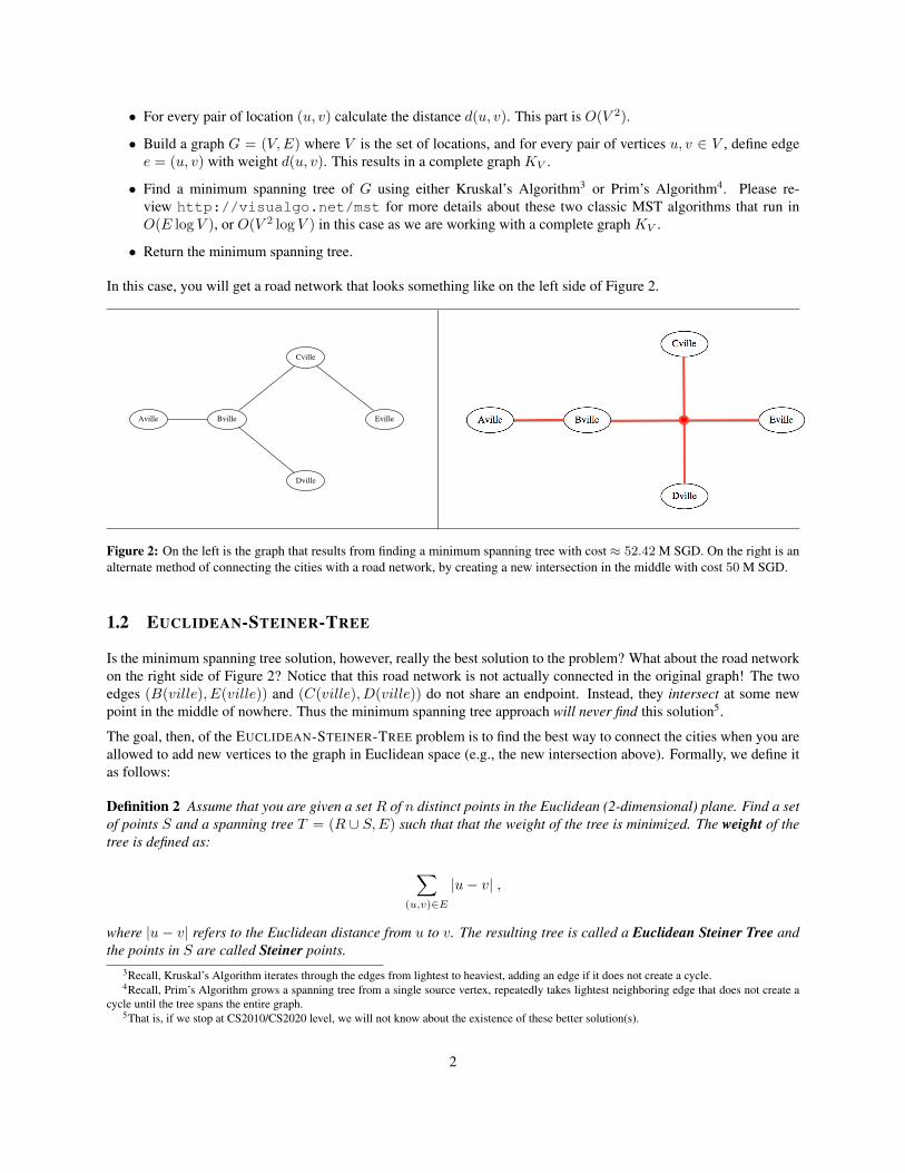
In this case, you will get a road network that looks something like on the left side of Figure 2.

������ ������

������

������

������

Figure 2: On the left is the graph that results from finding a minimum spanning tree with cost ≈ 52.42 M SGD. On the right is analternate method of connecting the cities with a road network, by creating a new intersection in the middle with cost 50 M SGD.

1.2 EUCLIDEAN-STEINER-TREE

Is the minimum spanning tree solution, however, really the best solution to the problem? What about the road networkon the right side of Figure 2? Notice that this road network is not actually connected in the original graph! The twoedges (B(ville), E(ville)) and (C(ville), D(ville)) do not share an endpoint. Instead, they intersect at some newpoint in the middle of nowhere. Thus the minimum spanning tree approach will never find this solution5.

The goal, then, of the EUCLIDEAN-STEINER-TREE problem is to find the best way to connect the cities when you areallowed to add new vertices to the graph in Euclidean space (e.g., the new intersection above). Formally, we define itas follows:

Definition 2 Assume that you are given a set R of n distinct points in the Euclidean (2-dimensional) plane. Find a setof points S and a spanning tree T = (R ∪ S,E) such that that the weight of the tree is minimized. The weight of thetree is defined as:

∑(u,v)∈E

|u− v| ,

where |u− v| refers to the Euclidean distance from u to v. The resulting tree is called a Euclidean Steiner Tree andthe points in S are called Steiner points.

3Recall, Kruskal’s Algorithm iterates through the edges from lightest to heaviest, adding an edge if it does not create a cycle.4Recall, Prim’s Algorithm grows a spanning tree from a single source vertex, repeatedly takes lightest neighboring edge that does not create a

cycle until the tree spans the entire graph.5That is, if we stop at CS2010/CS2020 level, we will not know about the existence of these better solution(s).

2

As you can see above, adding new points to the graph can results in a spanning tree of lower cost than just the standardminimum spanning tree result! The goal of the EUCLIDEAN-STEINER-TREE problem is to determine how much wecan reduce the cost.

Unlike the MIN-SPANNING-TREE problem, finding the minimum solution for EUCLIDEAN-STEINER-TREE problemis NP-hard [1]. Unfortunately we do not have an easy-to-describe-yet-reasonably-good algorithm for this variant,so we will not discuss this variant in depth. We do, however, know some facts about the structure of any optimalEuclidean Steiner Tree:

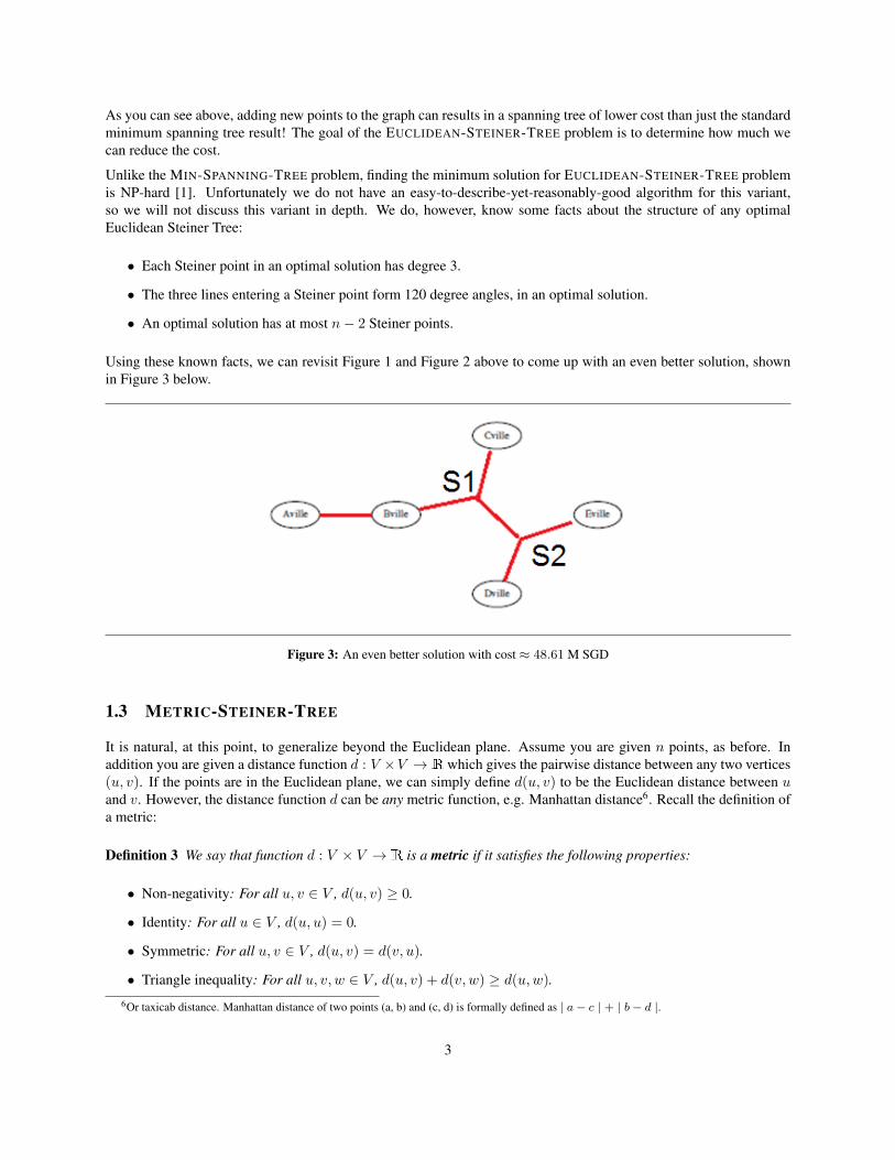
• Each Steiner point in an optimal solution has degree 3.

• The three lines entering a Steiner point form 120 degree angles, in an optimal solution.

• An optimal solution has at most n− 2 Steiner points.

Using these known facts, we can revisit Figure 1 and Figure 2 above to come up with an even better solution, shownin Figure 3 below.

Figure 3: An even better solution with cost ≈ 48.61 M SGD

1.3 METRIC-STEINER-TREE

It is natural, at this point, to generalize beyond the Euclidean plane. Assume you are given n points, as before. Inaddition you are given a distance function d : V ×V → R which gives the pairwise distance between any two vertices(u, v). If the points are in the Euclidean plane, we can simply define d(u, v) to be the Euclidean distance between uand v. However, the distance function d can be any metric function, e.g. Manhattan distance6. Recall the definition ofa metric:

Definition 3 We say that function d : V × V → R is a metric if it satisfies the following properties:

• Non-negativity: For all u, v ∈ V , d(u, v) ≥ 0.

• Identity: For all u ∈ V , d(u, u) = 0.

• Symmetric: For all u, v ∈ V , d(u, v) = d(v, u).

• Triangle inequality: For all u, v, w ∈ V , d(u, v) + d(v, w) ≥ d(u,w).6Or taxicab distance. Manhattan distance of two points (a, b) and (c, d) is formally defined as | a− c | + | b− d |.

3

(Technically, this is often referred to as a pseudometric, since we allow distances d(u, v) for u 6= v to equal 0.) Thekey aspect of the distance function d is that it must satisfy the triangle inequality.

If we want to think of the input as a graph, we can define G = (V,E) where V is the set of points, and E is the set ofall(n2

)pairs of edges, where the weight of edge (u, v) is equal to d(u, v).

As in the Euclidean case, we can readily find a minimum spanning tree ofG. However, the STEINER-TREE problem isto find if there is any better network, if we are allowed to add additional points. Unlike in the Euclidean case, however,it is not immediately clear which points can be added. Therefore, we are also given a set S of possible Steiner pointsto add. The goal is to choose some subset of S to minimize the cost of the spanning tree. The Metric Steiner Treeproblem is defined more precisely as follows:

Definition 4 Assume we are given:

• A set of required vertices R,

• A set of Steiner vertices S,

• A distance function d : (R ∪ S)× (R ∪ S)→ R that is a distance metric on the points in R and S.

The METRIC-STEINER-TREE problem is to find a subset S′ ⊂ S of the Steiner vertices and a spanning tree T =(R ∪ S′, E) of minimum weight. The weight of the tree T = (R ∪ S′, E) is defined to be:

∑(u,v)∈E

d(u, v) .

1.4 GENERAL-STEINER-TREE

At this point, we can generalize even further to the case where d is not a distance metric. Instead, assume that we aresimply given an arbitrary graph with edge weights, where some of the vertices are required vertices and some of thevertices are Steiner vertices.

Definition 5 Assume we are given:

• a graph G = (V,E),

• edge weights w : E → R,

• a set of required vertices R ⊆ V ,

• a set of Steiner vertices S ⊆ V .

Assume that V = R ∪ S. The GENERAL-STEINER-TREE problem is to find a subset S′ ⊂ S of the Steiner verticesand a spanning tree T = (R ∪ S′, E) of minimum weight. The weight of the tree T = (R ∪ S′, E) is defined to be:

∑(u,v)∈E

d(u, v) .

4

1.5 Summarizing the Three Different Variants

So far, we have defined three variants of the STEINER-TREE problem:

• Euclidean: The first variant assumes that we are considering points in the Euclidean plane.

• Metric: The second variant assumes that we have a distance metric.

• General: The third variant allows for an arbitrary graph.

Notice that the GENERAL-STEINER-TREE problem is clearly a generalization of the METRIC-STEINER-TREE prob-lem. On the other hand, if the set of Steiner points/vertices is restricted to be finite (or countable)7, then the METRIC-STEINER-TREE problem is not simply a generalization of the EUCLIDEAN-STEINER-TREE problem as the EUCLIDEAN-STEINER-TREE problem allows any points in the plane to be a Steiner point!

All the variants of the problem are relatively important in practice. In almost any network design problem, we arereally interested in Steiner Trees, not simply Minimum Spanning Trees8. (One common example is VLSI layout,where we need to route wires between components on the chip.)

All three variants of the problem are NP-hard [1].

2 Steiner Tree Approximations: OK and Bad Examples

There is a simple and natural heuristic for solving the Steiner Tree problem: Just ignore all the Steiner vertices andsimply find a minimum spanning tree for the required vertices R. Does this find a good approximation? We will seethat for the Euclidean Steiner Tree problem and the Metric Steiner Tree problem, an MST is a good approximation ofthe optimal Steiner Tree. However, for the General Steiner Tree problem, an MST is not a good approximation.

First, consider this example of the Euclidean Steiner Tree problem:

On the left picture, we are given an equilateral triangle with side-length 1. The minimum spanning tree for this triangleincludes any two of the edges, and hence has length 2 (as in the middle). However, the minimum Steiner tree for thetriangle adds one Steiner point: The point in the middle of the triangle (as on the right picture). With this extra Steinerpoint, now the total cost is

√(3). (You can calculate this based on the fact that the angle in the middle is 120 degrees.)

Thus, a minimum spanning tree is, at best, a 2/√

(3)-approximation (or 1.15-approximation) of the optimal EuclideanSteiner tree. Is it always at least a 2/

√(3)-approximation of optimal? That remains an open conjecture. As of today,

no one knows of any example that is worse than the triangle.

Now consider the Metric Steiner Tree problem. Obviously, a minimum spanning tree still cannot be better than a2/√(3)-approximation, since again we could consider the triangle with a single Steiner point in the middle. Now,

however, we can construct a better example.

7Which actually makes the STEINER-TREE problem ‘easier’...8So technically, stopping at CS2010/CS2020 level is not really enough to deal with these kinds of problems :O...

5

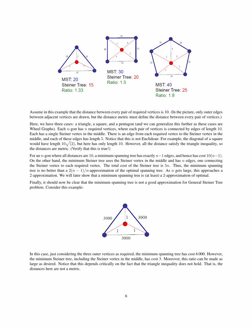
Assume in this example that the distance between every pair of required vertices is 10. (In the picture, only outer edgesbetween adjacent vertices are drawn, but the distance metric must define the distance between every pair of vertices.)

Here, we have three cases: a triangle, a square, and a pentagon (and we can generalize this further as these cases areWheel Graphs). Each n-gon has n required vertices, where each pair of vertices is connected by edges of length 10.Each has a single Steiner vertex in the middle. There is an edge from each required vertex to the Steiner vertex in themiddle, and each of these edges has length 5. Notice that this is not Euclidean: For example, the diagonal of a squarewould have length 10

√(2), but here has only length 10. However, all the distance satisfy the triangle inequality, so

the distances are metric. (Verify that this is true!)

For an n-gon where all distances are 10, a minimum spanning tree has exactly n−1 edges, and hence has cost 10(n−1).On the other hand, the minimum Steiner tree uses the Steiner vertex in the middle and has n edges, one connectingthe Steiner vertex to each required vertex. The total cost of the Steiner tree is 5n. Thus, the minimum spanningtree is no better than a 2(n − 1)/n-approximation of the optimal spanning tree. As n gets large, this approaches a2-approximation. We will later show that a minimum spanning tree is (at least) a 2-approximation of optimal.

Finally, it should now be clear that the minimum spanning tree is not a good approximation for General Steiner Treeproblem. Consider this example:

In this case, just considering the three outer vertices as required, the minimum spanning tree has cost 6 000. However,the minimum Steiner tree, including the Steiner vertex in the middle, has cost 3. Moreover, this ratio can be made aslarge as desired. Notice that this depends critically on the fact that the triangle inequality does not hold. That is, thedistances here are not a metric.

6

3 METRIC-STEINER-TREE Approximation Algorithm

We are now going to show that, in a metric space, a minimum spanning tree is a good approximation of a Steiner tree.This yields a simple algorithm for finding an approximately optimal Steiner tree, in the metric case: Simply ignore theSteiner points and return the minimum spanning tree!

Theorem 6 For a set of required verticesR, a set of Steiner vertices S, and a metric distance function d, the minimumspanning tree of (R, d) is a 2-approximation of the optimal Steiner Tree for (R,S, d).

Proof Throughout the proof, we will use as an example the graph in Figure 4. Here we have a graph with sixrequired vertices (i.e., the blue ones) and two Steiner vertices (i.e., the red ones). All the edges drawn have distance 1;all the other edges (not drawn) have distance 2.

Figure 4: Example for showing that a minimum spanning tree is a 2-approximation of the optimal Steiner tree, if the distances area metric. Assume that all edges not drawn have distance 2. Verify that these distances satisfy the triangle inquality.

Let T = (V,E) be the optimal Steiner tree, for some V ⊆ R ∪ S. For our example, we have drawn this optimalSteiner tree in Figure 5.

Figure 5: Here we have drawn the optimal Steiner tree T of graph shown in Figure 4.

7

The first step of the proof is to transform the tree T into a cycle C of at most twice the cost. We accomplish thisby performing a DFS of the tree T , adding each edge to the cycle as it is traversed (both down and up). Notice thatthe cycle begins and ends at the root of the tree, and each edge appears in the cycle exactly twice: Once traversingdown from a parent to a child, and once traversing up from a child to a parent. (Also notice that this cycle visits somevertices multiple times: A vertex with x children in the tree will appear 2(x+ 1) times (2x for root vertex), twice foreach of the x+ 1 (x for root vertex) adjacent edges.)

In our example, the cycle C is as follows:

(a, g)→ (g, d)→ (d, g)→ (g, f)→ (f, g)→ (g, a)→ (a, h)→

(h, c)→ (c, h)→ (h, b)→ (b, h)→ (h, a)→ (a, e)→ (e, a)

Notice that this cycle has 14 edges, whereas the original tree has 7 edges and 8 vertices.

We have already defined the cost(T ) =∑

e∈E d(e). Similarly, the cost of cycle C is defined as cost(C) =∑e∈C d(e). Since every edge in the tree T appears exactly twice in the cycle C, we know that cost(C) = 2×cost(T ).

In our example, we see that the cost of the original tree T is 8 and the cost of the cycle C is 16.

The cycle C contains both required vertices in R and Steiner vertices in S. We now want to remove all the Steinervertices from C, without increasing the cost of the cycle C. Find any two consecutive edges in the cycle (u, v) and(v, w) where the intermediate vertex v is a Steiner vertex. (At this point, it does not matter whether u and w arerequired or Steiner). Replace the two edges (u, v) and (v, w) with a single edge (u,w), thus deleting the Steinervertex v. We refer to this procedure as “short-cutting v.” Notice that this replacement does not increase the cost of thecycle C, since d(u,w) ≤ d(u, v) + d(v, w)—by the triangle inequality. (Hint: Always pay attention to where we usethe assumption; here is where the proof depends on the triangle inequality.) Continue short-cutting Steiner verticesuntil all the Steiner vertices have been deleted from C.

In our example, the Steiner vertices to be removed are g and h. Thus, we update the cycle C as follows:

(a, d)→ (d, f)→ (f, a)→ (a, c)→ (c, b)→ (b, a)→ (a, e)→ (e, a)

This revised cycle now has cost9: 2 + 1 + 2 + 2 + 2 + 2 + 2 + 2 = 15, which is no greater than the original cost ofthe cycle C (which was 16).

We now have a cycle C where cost(C) ≤ 2 × cost(T ). (Notice that the cost may have decreased during the short-cutting process, but it could not have increased.) Moreover, this cycle visits every required vertex in R at least twice(and there are no Steiner vertices in the cycle). The next step is to remove duplicates. Beginning at the root, traversethe cycle labeling each vertex: The first time a vertex is visited, mark it new; mark every other instances of that vertexin the cycle as old. (But mark the root vertex visited at the beginning and end as new.) As with Steiner vertices, wenow short-cut all the old vertices: Find two edges (u, v) and (v, w) where v is an old vertex and replace those twoedges in the cycle with a single edge (u,w). As before, this does not increase the cost of the cycle.

In our example, the cycle C visits the vertices in the following order:

a→ d→ f→ a→ c→ b→ a→ e→ a

The new vertices are colored with blue color, including vertex a at the beginning and the end. The old vertices arecolored with red color and underlined. This leaves two instances of vertex a to be shortcut. Once we shortcut past theold vertices, we are left with the following cycle C:

(a, d)→ (d, f)→ (f, c)→ (c, b)→ (b, e)→ (e, a)

9When you compute the new cost, refer to the cost in original Figure 4. For example, there is an edge with weight 1 that connects vertex d and fin Figure 4.

8

This cycle has cost10: 2 + 1 + 2 + 2 + 2 + 2 = 11, which is no greater than the original cost of the cycle (which was16). This revised cycle C is depicted in Figure 6.

Figure 6: Here we have drawn the cycle C after the Steiner vertices have been short-cut and the repeated vertices have been deleted.

We now have a cycle C where cost(C) ≤ 2 × cost(T ), and each required vertex in R appears exactly once. Finally,remove any one arbitrary edge from C. (Again, this cannot increase the cost of C.) At this point, C is a path whichtraverses each vertex in the graph exactly once. That is, C is a spanning tree with cost at most 2 × cost(T ). In ourexample, the spanning tree C (where one arbitrary edge (e.g. the last edge) of the cycle has been deleted is):

(a, d)→ (d, f)→ (f, c)→ (c, b)→ (b, e)

This is a spanning tree with cost 9.

Let M be the minimum spanning tree of the required vertices R. Since M is the spanning tree of minimum cost,clearly cost(M) ≤ cost(C) ≤ 2 × cost(T ). From this we conclude that M is a 2-approximation for the minimumcost Steiner tree of R ∪ S.

To summarize, the proof goes through the following steps:

1. Begin with the optimal Steiner Tree T .

2. Use a DFS traversal to generate a cycle of twice the cost.

3. Eliminate the Steiner vertices and repeated required vertices, without increasing the cost. (Use the assumptionthat d satisfies the triangle inequality.)

4. Remove on edge from the cycle, yielding a spanning tree of cost at most twice the cost of T .

5. Observe that the minimum spanning tree can have cost no greater than the constructed spanning tree, and henceno greater than twice the cost of T .

This implies that the minimum spanning tree has cost at most twice the cost of T , the optimal Steiner Tree.10Again, when you compute the new cost, refer to the cost in original Figure 4. For example, there are edges with weight 2 that connects vertex f

and c, vertex b and e, and vertex e and a in Figure 4 (all not drawn).

9

4 GENERAL-STEINER-TREE Approximation Algorithm

In general, a minimum spanning tree is not a good approximation for the GENERAL-STEINER-TREE problem. Herewe want to show how to find a good approximation in this case. Instead of developing an algorithm from scratch,we are going to use a reduction. Part of the goal is to demonstrate how to use reductions when we are talking aboutapproximation algorithms.

The typical process, with a reduction, is something like as follows:

• Begin with an instance of the GENERAL-STEINER-TREE problem.

• Via the reduction, construct a new instance of the METRIC-STEINER-TREE problem.

• Solve the METRIC-STEINER-TREE problem using our existing algorithm.

• Convert the solution to the METRIC-STEINER-TREE instance back to a solution for the GENERAL-STEINER-TREE problem.

The key to the analysis would typically be a lemma that says something like, “If we have an algorithm for finding anoptimal solution to the METRIC-STEINER-TREE problem, then our construction/conversion process yields an optimalsolution to the GENERAL-STEINER-TREE problem.”

With approximation algorithms, however, you have to be a little more careful. Normally, it is sufficient to show that anoptimal solution to the translated problem yields an optimal solution to the original problem. However, we are lookinghere at approximation algorithms. Hence we need to show that, even though we are only finding an approximatesolution to the METRIC-STEINER-TREE problem, that still yields an approximate solution to the GENERAL-STEINER-TREE problem. A reduction that preserves approximation ratios is known as a gap-preserving reduction.

Assume we are given a graph G = (V,E) and non-negative edge weights w : E → R≥0. The vertices V are

divided into required vertices R and Steiner vertices S. Our goal is to find a minimum cost Steiner Tree. There are norestrictions on the weights w (i.e., they do not necessarily satisfy the triangle inequality).

Defining a metric. In order to perform the reduction, we need to construct an instance of the METRIC-STEINER-TREE problem. In particular, we need to define a metric. The specific distance metric we are going to define is knownas the metric completion of G.

Definition 7 Given a graph G = (V,E) and non-negative edge weights w, we define the metric completion of G tothe be the distance function d : V × V → R constructed as follows: For every u, v ∈ V , define d(u, v) to be thedistance of the shortest path from u to v in G with respect to the weight function w.

Notice that the metric completion d provides distances between every pair of vertices, not just the edges in E. Alsonotice that, computationally, d is relatively easy to calculate, e.g., via an All-Pairs-Shortest-Paths algorithm such asFloyd-Warshall which runs in O(V 3) time11. Critically, d is a metric:

Lemma 8 Given a graph G = (V,E), the metric completion d is a metric with respect to V .

Proof Since all the edge weights are non-negative, clearly d(u, v) ≥ 0 for all u, v ∈ V . Similarly, d(u, u) = 0, bydefinition. Since the original graph is undirected, the shortest path from u to v is also the shortest path from v to u;hence d(u, v) = d(v, u).

11Compared to the NP-hardness of the original STEINER-TREE problem, running an O(V 3) algorithm for its approximation algorithm is gener-ally viewed as OK.

10

The most interesting property is the triangle inequality. We need to show that for all vertices u, v, w ∈ V , thedistances d(u, v) + d(v, w) ≥ d(u,w). Assume, for the sake of contradiction, that this inequality does not hold, i.e.,d(u, v)+d(v, w) < d(u,w). Let Pu,v be the shortest path from u to v inG (with respect to the weight functionw), andlet Pv,w be the shortest path from v to w (with respect to the weight function w). Consider the path Pu,v+Pv,w, whichis a path from u to w of length d(u, v) + d(v, w). This path is of length less than d(u,w). But that is a contradiction,since d(u,w) was defined to be the length of the shortest path from u to w.

From this, we conclude that d satisfies the triangle inequality, and hence is a metric.

In the following, we will sometimes be calculating the cost with respect to the metric completion d, and sometimeswith respect to the edge weights w. To be clear, we will use costd to refer to the former and costw to refer to thelatter. Similarly, we will refer to graph Gg when talking about the GENERAL-STEINER-TREE problem, and Gm whentalking about the METRIC-STEINER-TREE problem.

Converting from General to Metric. We can now reduce the original instance of the GENERAL-STEINER-TREEproblem to an instance of the METRIC-STEINER-TREE problem. Assume we have an algorithm A that finds anα-approximate minimum cost METRIC-STEINER-TREE.

• Given a graph Gg = (V,Eg) with requires vertices R, Steiner vertices S, and a non-negative edge weightfunction w:

• Let d be the metric completion of Gg .

• Consider the METRIC-STEINER-TREE problem: (R,S, d).

• Let Tm = A(R,S, d) be the α-approximate minimum cost Metric Steiner tree.

At this point, we have converted our GENERAL-STEINER-TREE problem into a METRIC-STEINER-TREE problem,and solved it using our existing approximation algorithm.

Converting from Metric back to General. We are not yet done, however, since Tm is defined in terms of edgesthat may not exist in Gg , and in terms of a different set of costs. We need to convert the tree Tm back into a tree inGg .

For every edge e = (u, v) in the tree Tm, let pe be the shortest path in Gg from u to v. Let P =⋃

e∈T pe, i.e., the setof all paths that make up the tree Tm. Notice that some of these paths may overlap.

Define the cost of a path in Gg (with respect to w) to be the sum of the costs of the edge weights, i.e., costw(p) =∑e∈p w(e). Notice that the cost of a path in Gg is with respect to edge weights, while the cost of the tree Tm is with

respect to the metric completion d. (This difference is because we are converting back from the metric to the generalproblem.) If e = (u, v) is an edge in the tree Tm, then costw(pe) = d(u, v).

Consider all the paths pe ∈ P , i.e., for every edge e in the tree Tm: add every edge that appears in any path pe ∈ P toa set E′. Notice that the graph G′ = (V,E′) is connected, since the original tree Tm was connected and if there wasan edge (u, v) in Tm then there is a path connecting u to v in E′. Also, notice that the cost of all the edges in E′ (withrespect to w) is no greater than the cost of all the edges in Tm (with respect to d), since each path pe costs the sameamount as the edge e in Tm.

Finally, we need to remove any cycles from the graph (V,E′) so that we have a spanning tree. Let T g be the minimumspanning of (V,E′). The tree T g in the graph Gg = (V,Eg) with edge weights w has cost no greater than the tree Tm

with edge weights d.

11

Analysis. To analyze this, we need to prove two key lemmas (proof omitted). Notice that you need to prove twothings: You need to relate the solution in the metric version to OPT in the general version, and you also need to relatethe final solution in the general version to the solution found in the metric version.

Lemma 9 Let OPT g be the optimal minimum cost Steiner tree for Gg . Then costd(Tm) ≤ α · costw(OPT g).

Lemma 10 Let T g be the Steiner tree calculated by converting Tm back to graphGg . Then costw(T g) ≤ costd(Tm)

Putting these lemmas together, we get our final result:

Theorem 11 Given anα-approximation algorithm for METRIC-STEINER-TREE problem, we can find anα-approximationfor a GENERAL-STEINER-TREE problem.

Proof Assume we have a graph Gg = (V,Eg) with required vertices R, Steiner vertices S, and a non-negativeedge weight function w. Let Tm be an α-approximate Steiner tree for (R,S, d), where d is the metric completion ofGg . Let T g be the spanning tree constructed above by converting the edges in Tm into paths in Gg = (V,Eg) andremoving cycles. We will argue that T g is an α-approximation of the minimum cost spanning tree for G.

First, we have shown that costd(Tm) ≤ α · costw(OPT g). Second, we have shown that costw(T g) ≤ costd(Tm).

Putting the two pieces together, we conclude that costw(T g) ≤ α·costw(OPT g), and hence T g is an α-approximationfor the minimum cost Steiner tree for G with respect to w.

References

[1] Michael R. Garey and David S. Johnson. Computers and Intractability: A Guide to the Theory of NP-Completeness. W.H. Freeman and Company, 1979.

12

IndexApproximation Algorithm, 7, 10

Euclidean-Steiner-Tree, 2

Gap-Preserving Reduction, 10General Steiner Tree

Approximation Algorithm, 10General-Steiner-Tree, 4

Kruskal’s Algorithm, 2

Metric, 3Metric Steiner Tree

Approximation Algorithm, 7Metric-Steiner-Tree, 3Min-Spanning-Tree, 1Min-Steiner-Tree, see Steiner-Tree

Prim’s Algorithm, 2

Required Vertices, 4

Steiner Points, 2Steiner Vertices, 4Steiner-Tree, 1

Bad Approximation, 5Euclidean, 2General, 4Metric, 3OK Approximation, 5

Wheel Graph, 6

13