PGM 2002/03 Tirgul5

Clique/Junction Tree Inference

Outline In class we saw how to construct junction tree via graph theoretic prinicipals In the last tirgul we saw the algebric connection between elimination and message propagation

In this tirgul we will see how elimination in a general graph implies a triangulation and a junction tree and use this to define a practical algrithm for exact inference in general graphs

Undirected graph representation

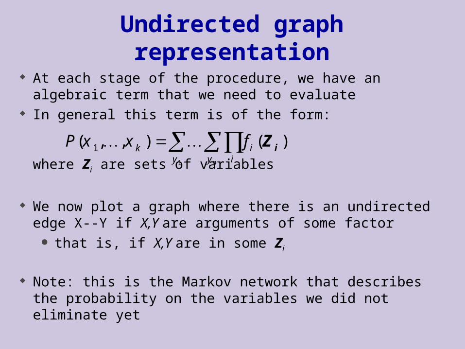
At each stage of the procedure, we have an algebraic term that we need to evaluate

In general this term is of the form:

where Zi are sets of variables

We now plot a graph where there is an undirected edge X--Y if X,Y are arguments of some factor

that is, if X,Y are in some Zi

Note: this is the Markov network that describes the probability on the variables we did not eliminate yet

1

)(),,( 1y y i

ikn

fxxP iZ

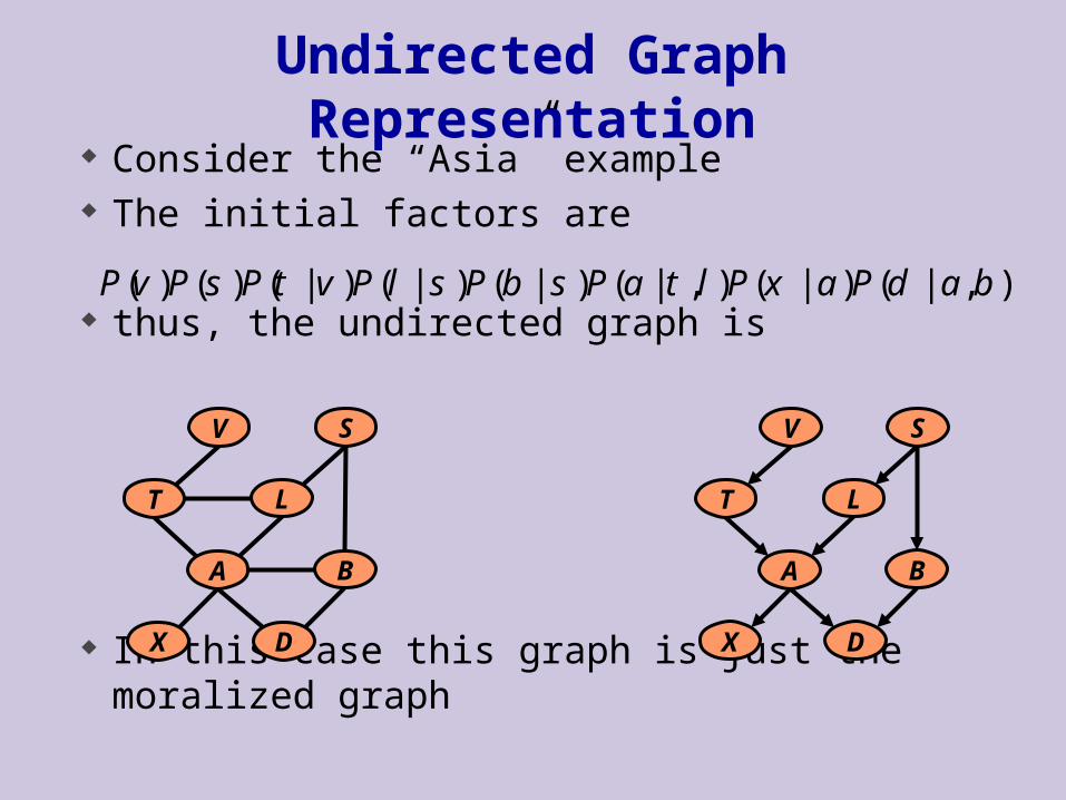
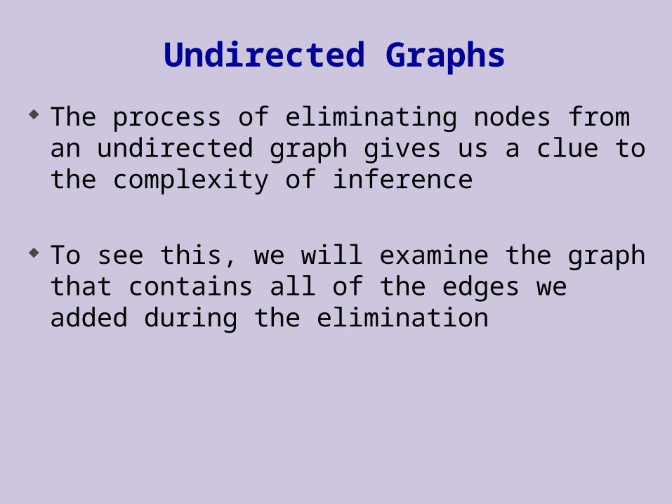
Undirected Graph Representation Consider the “Asia” example The initial factors are

thus, the undirected graph is

In this case this graph is just the moralized graph

),|()|(),|()|()|()|()()( badPaxPltaPsbPslPvtPsPvP

V S

LT

A B

X D

V S

LT

A B

X D

Elimination in Undirected Graphs

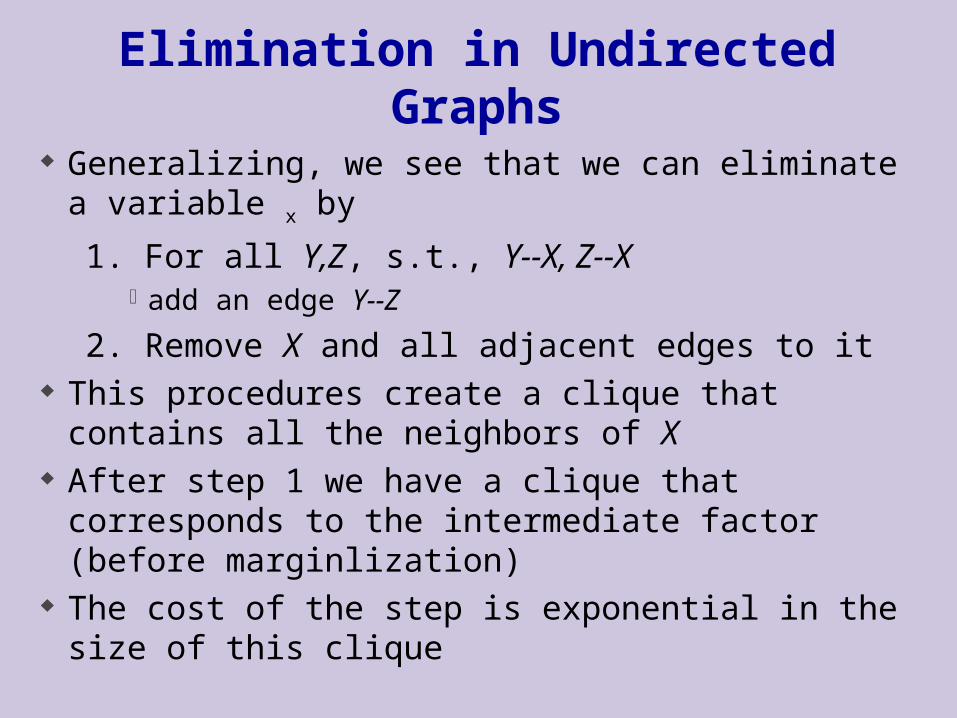
Generalizing, we see that we can eliminate a variable x by

1. For all Y,Z, s.t., Y--X, Z--Xadd an edge Y--Z

2. Remove X and all adjacent edges to it This procedures create a clique that contains all the

neighbors of X After step 1 we have a clique that corresponds to

the intermediate factor (before marginlization) The cost of the step is exponential in the size of this

clique

Undirected Graphs

The process of eliminating nodes from an undirected graph gives us a clue to the complexity of inference

To see this, we will examine the graph that contains all of the edges we added during the elimination

Example

Want to compute P(L)

Moralizing

V S

LT

A B

X D

LT

A B

X

V S

D

Example

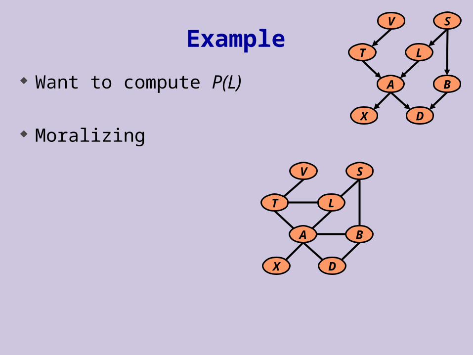
Want to compute P(L)

Moralizing Eliminating v

Multiply to get f’v(v,t) Result fv(t)

V S

LT

A B

X D

LT

A B

X

V S

D

Example

Want to compute P(L)

Moralizing Eliminating v Eliminating x

Multiply to get f’x(a,x) Result fx(a)

V S

LT

A B

X D

LT

A B

X

V S

D

Example

Want to compute P(L)

Moralizing Eliminating v Eliminating x Eliminating s

Multiply to get f’s(l,b,s) Result fs(l,b)

V S

LT

A B

X D

LT

A B

X

V S

D

Example

Want to compute P(D)

Moralizing Eliminating v Eliminating x Eliminating s Eliminating t

Multiply to get f’t(a,l,t) Result ft(a,l)

V S

LT

A B

X D

LT

A B

X

V S

D

Example

Want to compute P(D)

Moralizing Eliminating v Eliminating x Eliminating s Eliminating t Eliminating l

Multiply to get f’l(a,b,l) Result fl(a,b)

V S

LT

A B

X D

LT

A B

X

V S

D

Example

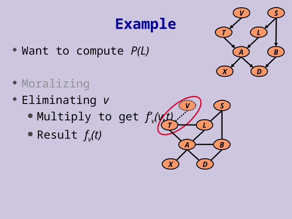
Want to compute P(D)

Moralizing Eliminating v Eliminating x Eliminating s Eliminating t Eliminating l Eliminating a, b

Multiply to get f’a(a,b,d) Result f(d)

V S

LT

A B

X D

LT

A B

X

V S

D

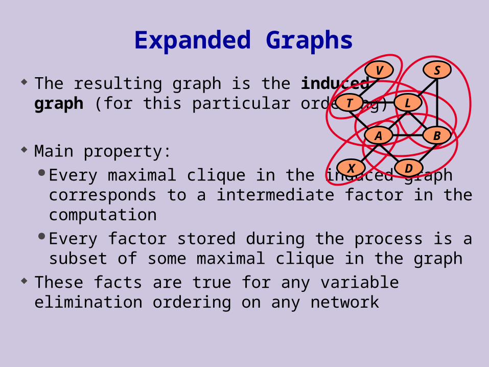
The resulting graph is the inducedgraph (for this particular ordering)

Main property: Every maximal clique in the induced graph

corresponds to a intermediate factor in the computation

Every factor stored during the process is a subset of some maximal clique in the graph

These facts are true for any variable elimination ordering on any network

Expanded Graphs

LT

A B

X

V S

D

Induced Width

The size of the largest clique in the induced graph is thus an indicator for the complexity of variable elimination

This quantity is called the induced width of a graph according to the specified ordering

Finding a good ordering for a graph is equivalent to finding the minimal induced width of the graph

Chordal Graphs Recall:

elimination ordering undirected chordal graph

Graph: Maximal cliques are factors in elimination Factors in elimination are cliques in the graph Complexity is exponential in size of the largest

clique in graph

LT

A B

X

V S

D

V S

LT

A B

X D

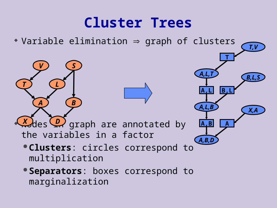
Cluster Trees Variable elimination graph of clusters

Nodes in graph are annotated by the variables in a factor Clusters: circles correspond to multiplication Separators: boxes correspond to marginalization

V S

LT

A B

X D

T,V

A,L,TB,L,S

X,AA,L,B

A,B,D

AA,B

B,L

T

A,L

Properties of cluster trees

Cluster graph must be a tree Only one path between any

two clusters

A separator is labeled by the intersection of the labels of the two neighboring clusters

Running intersection property: All separators on the path between

two clusters contain their intersection

T,V

A,L,TB,L,S

X,AA,L,B

A,B,D

AA,B

B,L

T

A,L

Cluster Trees & Chordal Graphs

Combining the two representations we get that: Every maximal clique in chordal is a cluster in

tree Every separator in tree is a separator in the

chordal graph

LT

A B

X

V S

D

T,V

A,L,T B,L,S

X,AA,L,B

A,B,D

AA,B

B,L

T

A,L

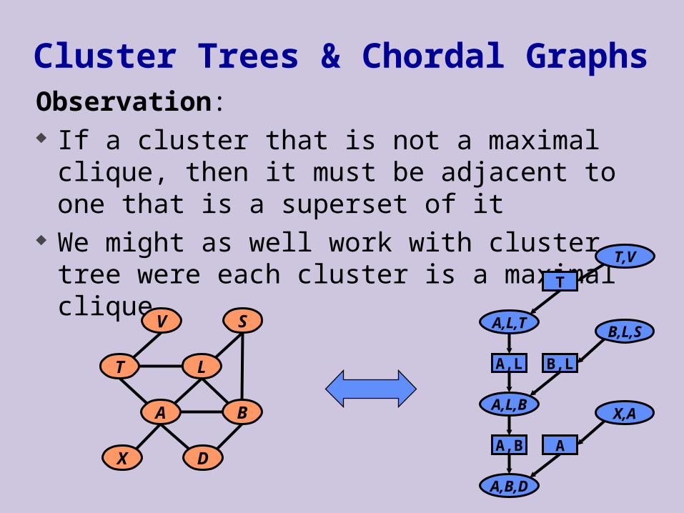
Cluster Trees & Chordal GraphsObservation: If a cluster that is not a maximal clique, then it

must be adjacent to one that is a superset of it We might as well work with cluster tree were each

cluster is a maximal clique

LT

A B

X

V S

D

T,V

A,L,TB,L,S

X,AA,L,B

A,B,D

AA,B

B,L

T

A,L

Cluster Trees & Chordal Graphs

Thm: If G is a chordal graph, then it can be embedded in

a tree of cliques such that: Every clique in G is a subset of at least one

node in the tree The tree satisfies the running intersection

property

Elimination in Chordal Graphs A separator S divides the remaining

variables in the graph in to two groups Variables in each group appears on

one “side” in the cluster tree

Examples: {A,B}: {L, S, T, V} & {D, X} {A,L}: {T, V} & {B,D,S,X} {B,L}: {S} & {A, D,T, V, X} {A}: {X} & {B,D,L, S, T, V} {T}; {V} & {A, B, D, K, S, X}

LT

A B

X

V S

D

T,V

A,L,T B,L,S

X,AA,L,B

A,B,D

AA,B

B,L

T

A,L

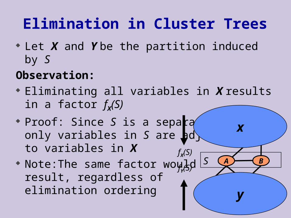
Elimination in Cluster Trees Let X and Y be the partition induced by SObservation: Eliminating all variables in X results in a factor

fX(S) Proof: Since S is a separator

only variables in S are adjacentto variables in X

Note:The same factor would result, regardless of elimination ordering

x

y

A BSfX(S)

fY(S)

Recursive Elimination in Cluster Trees

How do we compute fX(S) ? By recursive decomposition along

cluster tree Let X1 and X2 be the disjoint

partitioning of X - C implied by theseparators S1 and S2

Eliminate X1 to get fX1(S1) Eliminate X2 to get fX2(S2) Eliminate variables in C - S to

get fX(S)

C

S

S2S1

x1

x2

y

Elimination in Cluster Trees(or Belief Propagation revisited)

Assume we have a cluster tree Separators: S1,…,Sk

Each Si determines two sets of variables Xi and Yi, s.t.

Si Xi Yi = {X1,…,Xn} All paths from clusters containing variables in

Xi to clusters containing variables in Yi pass through Si

We want to compute fXi(Si) and fYi(Si) for all i

Elimination in Cluster TreesIdea: Each of these factors can be decomposed as an

expression involving some of the others Use dynamic programming to avoid

recomputation of factors

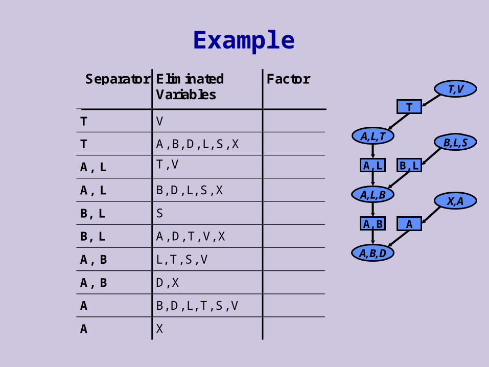
Example

T,V

A,L,T B,L,S

X,AA,L,B

A,B,D

AA,B

B,L

T

A,L

Separator EliminatedVariables

Factor

T V

T A, B, D, L, S, X

A, L T, V

A, L B, D, L, S, X

B, L S

B, L A, D, T, V, X

A, B L, T, S, V

A, B D, X

A B, D, L, T, S, V

A X

Dynamic Programming

We now have the tools to solve the multi-query problem

Step 1: Inward propagation Pick a cluster C Compute all factors eliminating from

fringes of the tree toward C This computes all “inward” factors

associated with separatorsC

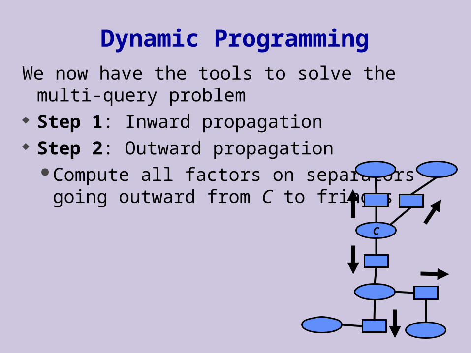
Dynamic Programming

We now have the tools to solve the multi-query problem

Step 1: Inward propagation Step 2: Outward propagation

Compute all factors on separators going outward from C to fringes

C

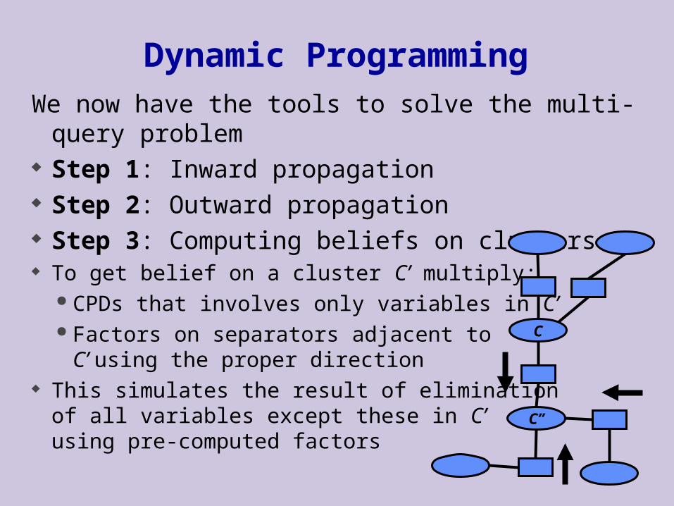
Dynamic ProgrammingWe now have the tools to solve the multi-query

problem Step 1: Inward propagation Step 2: Outward propagation Step 3: Computing beliefs on clusters To get belief on a cluster C’ multiply:

CPDs that involves only variables in C’ Factors on separators adjacent to

C’ using the proper direction This simulates the result of elimination

of all variables except these in C’using pre-computed factors

C

C’’

Complexity

Time complexity: Each traversal of the tree is costs the same as

standard variable elimination Total computation cost is twice of standard variable

elimination

Space complexity: Need to store partial results Requires two factors for each separator Space requirements can be up to 2n more expensive

than variable elimination

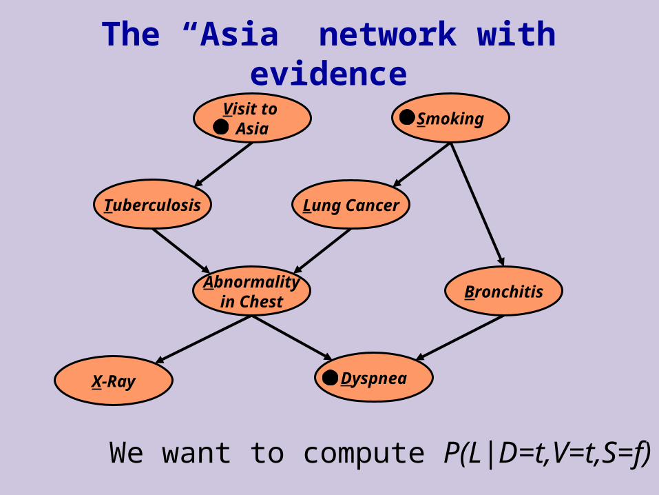
The “Asia” network with evidence

Visit to Asia

Smoking

Lung CancerTuberculosis

Abnormalityin Chest

Bronchitis

X-Ray Dyspnea

We want to compute P(L|D=t,V=t,S=f)

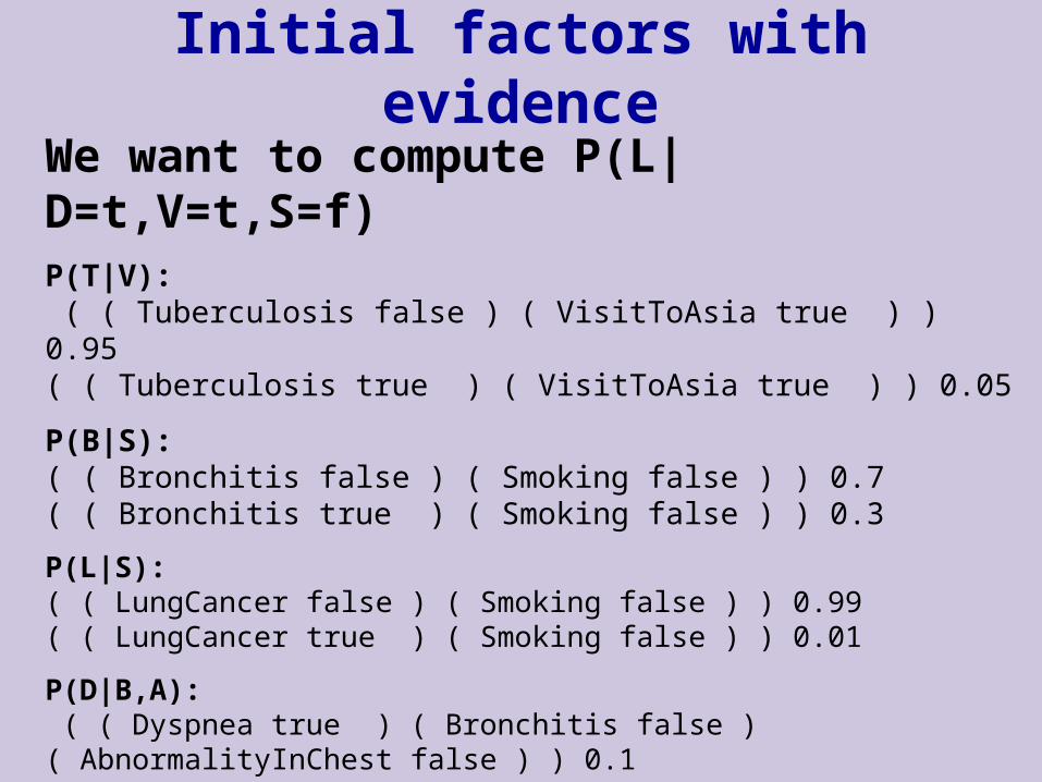
Initial factors with evidence

We want to compute P(L|D=t,V=t,S=f)P(T|V): ( ( Tuberculosis false ) ( VisitToAsia true ) ) 0.95( ( Tuberculosis true ) ( VisitToAsia true ) ) 0.05

P(B|S):( ( Bronchitis false ) ( Smoking false ) ) 0.7 ( ( Bronchitis true ) ( Smoking false ) ) 0.3

P(L|S):( ( LungCancer false ) ( Smoking false ) ) 0.99 ( ( LungCancer true ) ( Smoking false ) ) 0.01

P(D|B,A): ( ( Dyspnea true ) ( Bronchitis false ) ( AbnormalityInChest false ) ) 0.1 ( ( Dyspnea true ) ( Bronchitis true ) ( AbnormalityInChest false ) ) 0.8 ( ( Dyspnea true ) ( Bronchitis false ) ( AbnormalityInChest true ) ) 0.7 ( ( Dyspnea true ) ( Bronchitis true ) ( AbnormalityInChest true ) ) 0.9

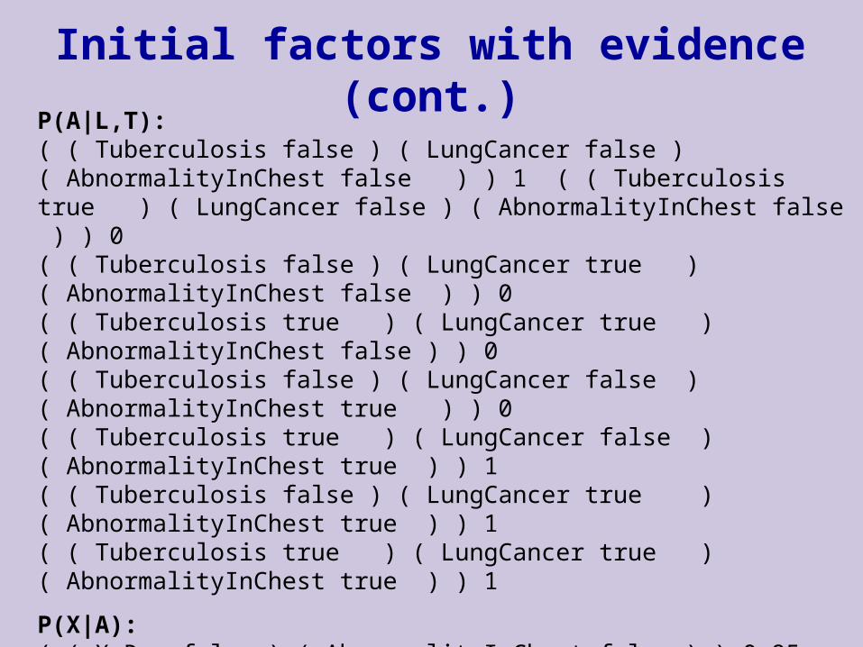
Initial factors with evidence (cont.)P(A|L,T):( ( Tuberculosis false ) ( LungCancer false ) ( AbnormalityInChest false ) ) 1 ( ( Tuberculosis true ) ( LungCancer false ) ( AbnormalityInChest false ) ) 0 ( ( Tuberculosis false ) ( LungCancer true ) ( AbnormalityInChest false ) ) 0 ( ( Tuberculosis true ) ( LungCancer true ) ( AbnormalityInChest false ) ) 0

( ( Tuberculosis false ) ( LungCancer false ) ( AbnormalityInChest true ) ) 0 ( ( Tuberculosis true ) ( LungCancer false ) ( AbnormalityInChest true ) ) 1

( ( Tuberculosis false ) ( LungCancer true ) ( AbnormalityInChest true ) ) 1

( ( Tuberculosis true ) ( LungCancer true ) ( AbnormalityInChest true ) ) 1

P(X|A):( ( X-Ray false ) ( AbnormalityInChest false ) ) 0.95( ( X-Ray true ) ( AbnormalityInChest false ) ) 0.05 ( ( X-Ray false ) ( AbnormalityInChest true ) ) 0.02 ( ( X-Ray true ) ( AbnormalityInChest true ) ) 0.98

D,B,A

B,L,S

X,A

T,V

B,L,A

T,L,A

B,A

B,LL,A

A

T

Step 1: Initial Clique values

CT=P(T|V)

CT,L,A=P(A|L,T)

CB,L,A=1

CB,L=P(L|S)P(B|S)

CB,A=1

CX,A=P(X|A)

“dummy” separators: this is the intersection between nodes in the junction tree and helps in defining the inference messages (see below)

D,B,A

B,L,S

X,A

T,V

B,L,A

T,L,A

B,A

B,LL,A

A

T

Step 2: Update from leaves

S B,L=CB,L

ST=CT

S A=CX,A

CT

CT,L,A

CB,L,A

CB,L

CB,A

CX,A

D,B,A

B,L,S

X,A

T,V

B,L,A

T,L,A

B,A

B,LL,A

A

T

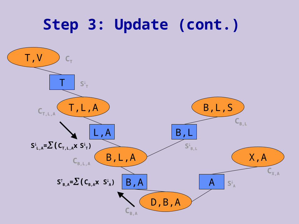
Step 3: Update (cont.)

SB,L

ST

CT

CT,L,A

CB,L,A

CB,L

CB,A

CX,A

SA

SB,A=(CB,Ax S

A)

SL,A=(CT,L,Ax S

T)

D,B,A

B,L,S

X,A

T,V

B,L,A

T,L,A

B,A

B,LL,A

A

T

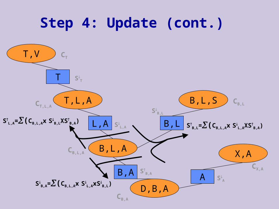
Step 4: Update (cont.)

SB,L

ST

SB,A

SL,A

CT

CT,L,A

CB,L,A

CB,L

CB,A

CX,A

SA

SB,A=(CB,L,Ax S

L,AxS

B,L)

SL,A=(CB,L,Ax S

B,LXS

B,A)S

B,L=(CB,L,Ax SL,AXS

B,A)

D,B,A

B,L,S

X,A

T,V

B,L,A

T,L,A

B,A

B,LL,A

A

T

Step 5: Update (cont.)

SB,L

ST

SB,A

SL,A

CT

CT,L,A

CB,L,A

CB,L

CB,A

CX,AS

A

SB,A

SL,A S

B,L

SA=(CB,Ax S

B,A)

ST=(CT,L,Ax S L,A)

D,B,A

B,L,S

X,A

T,V

B,L,A

T,L,A

B,A

B,LL,A

A

T

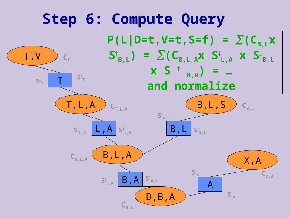
Step 6: Compute Query

SB,L

ST

SB,A

SL,A

CT

CT,L,A

CB,L,A

CB,L

CB,A

CX,AS

A

SB,A

SL,A S

B,L

SA

ST

P(L|D=t,V=t,S=f) = (CB,Lx SB,L) =

(CB,L,Ax SL,A x S

B,L x S B,A) = …and normalize

D,B,A

B,L,S

X,A

T,V

B,L,A

T,L,A

B,A

B,LL,A

A

T

How to avoid small numbers

SB,L

ST

SB,A

SL,A

CT

CT,L,A

CB,L,A

CB,L

CB,A

CX,A

SA

SB,A

SL,A S

B,L

SA

ST

P(L|D=t,V=t,S=f) = (CB,Lx SB,L) =

(CB,L,Ax SL,A x S

B,L x S B,A) = …

and normalize (with N1xN2xN3xN4xN5xNBLA)

Normalize by N1

Normalize by N3

Normalize by N2

Normalize by N4

Normalize by N5

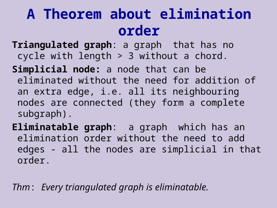
A Theorem about elimination order

Triangulated graph: a graph that has no cycle with length > 3 without a chord.

Simplicial node: a node that can be eliminated without the need for addition of an extra edge, i.e. all its neighbouring nodes are connected (they form a complete subgraph).

Eliminatable graph: a graph which has an elimination order without the need to add edges - all the nodes are simplicial in that order.

Thm: Every triangulated graph is eliminatable.

Lemma: An uncomplete triangulated graph G with a node set N (at least 3) has a complete subset S which separates the graph - every path between the two parts of N/S goes through S.

Proof: Let S be a minimal set of nodes such that any path between non-adjacent nodes A and B contains a nodes from S. Assume that C,D in S are not neighbors. Since S is minimal, there is a path from A to B in G passing only through C in S (and same for D). Then there is a path from C to D in GA and in GB. This path is a cycle that a chord C--D must break.

A BSG A G B

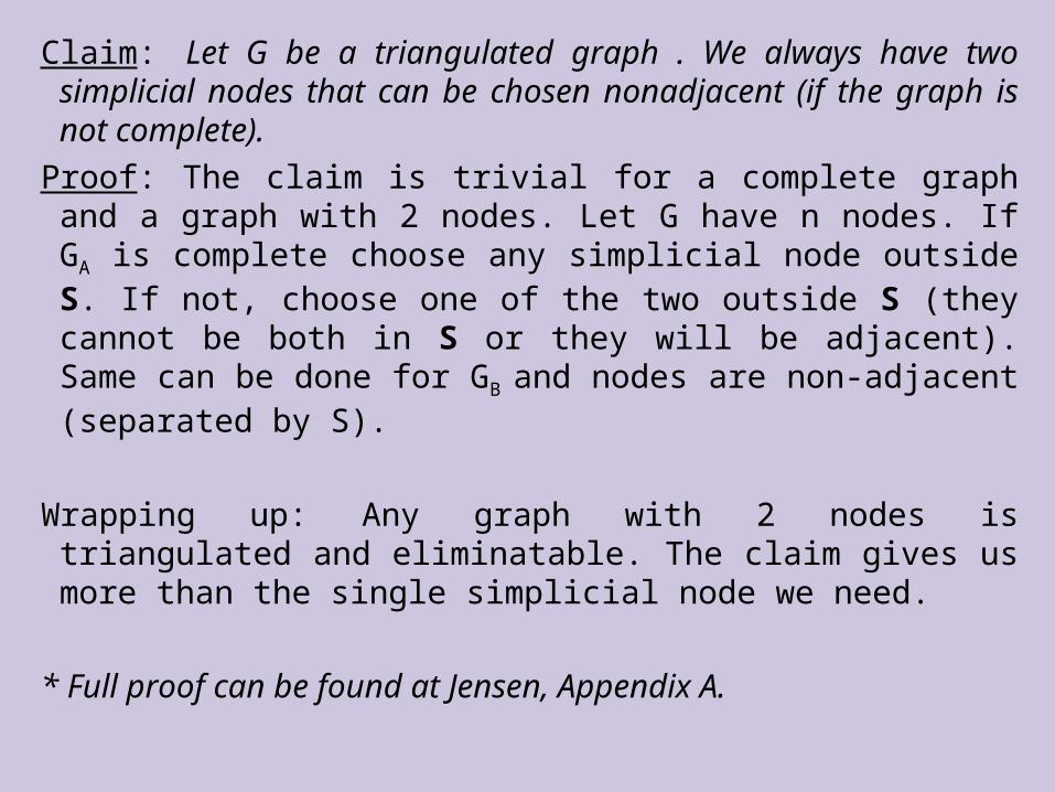
Claim: Let G be a triangulated graph . We always have two simplicial nodes that can be chosen nonadjacent (if the graph is not complete).

Proof: The claim is trivial for a complete graph and a graph with 2 nodes. Let G have n nodes. If GA is complete choose any simplicial node outside S. If not, choose one of the two outside S (they cannot be both in S or they will be adjacent). Same can be done for GB and nodes are non-adjacent (separated by S).

Wrapping up: Any graph with 2 nodes is triangulated and eliminatable. The claim gives us more than the single simplicial node we need.

* Full proof can be found at Jensen, Appendix A.