A Comparison Analysis on Decision Tree

Algorithms

Siyang Li and Shaoshan Zeng and Jiawen WuMathematics, Boston University

April 2021

Abstract

Decision trees are widely utilized in many fields for systematic prediction concern-ing classification and regression problems. One of the leading works of decision treetechniques is Classification and Regression Trees (CART) by Breiman et al. (1984).Some later proposals indicate the greedy nature and limitations of CART, seeking tominimize misclassification and the solving time for decision tree optimization. A newformulation for learning the optimal classification tree is proposed by Verwer and Zhang(2019) as a binary linear model called BinOCT. In this report, we compare BinOCTwith CART, Logistic regression, and Random Forests to examine if BinOCT actuallyachieves better accuracy within shorter solving time as claimed in Verwer and Zhang(2019). We perform our study on both small and large datasets, since the formulationsize of BinOCT is said to be largely independent from the training data size. Ourexperiment results show little but no significant improvements of BinOCT compared toCART, which fail to agree with Verwer and Zhang (2019). All four of our selected al-gorithms work better on smaller datasets with fewer number of features where LogisticRegression seems to be more stable and performs well on all datasets. For future direc-tion, we are interested in exploring hyper-parameters tuning as well as the performanceof BinOCT on large real-world datasets.

Keywords: BinOCT; CART; Random Forests; Logistic Regression.

1 Introduction

Decision trees are increasingly utilized in many fields, such as healthcare, for systematic

prediction concerning classification and regression problems. One of the leading proposals

of decision tree technniques is Classification and Regression Trees (CART) by Breiman et al.

(1984). A binary tree structured classifier conducts recursive categorization of targets based

on a set of specified measurements or variables. For instance, suppose S is a dimensional

feature space containing the measurement vectors s = ( s1, s2, ...) and that the targets or

training data fall into a given set of J number of classes C = { 1, 2, 3, . . . , J }. Each

1

subset of S is known as a node, and a decision tree with depth D has (2D+1–1) nodes. A

tree classifier, or classification rule, partitions S into J disjoint nodes such that every s is

assigned to one of the classes from C, i.e. { 1, 2, . . . J }. Compared to other statistical

classification methods, decision trees are favored for being very explicable, even though

numerically less accurate (Breiman 1984).

Prior to CART, ID3 (Iterative Dichotomiser 3) is a simple tree algorithm which con-

structs decision trees fast but suffers over-fitting (Quinlan, 1983). Later, IDX (Norton

1989) seeks to generate more logical and understandable decision trees compared to ID3

with quality addressed during the construction of decision trees. C4.5 (Salzberg, 1993)

is another updated version of ID3 that uses the concept of information entropy to deal

with both discrete and continuous attributes while creating trivial values in some nodes.

All of the above algorithms are considered greedy based heuristics, while LSID3 and ID3-

k (Esmeir and Markovitch 2007) claim to better solve this problem by slowing down its

computation speed for better quality called anytime induction algorithm.

Recently, there is a growing trend that utilizes mathematical optimization method for

decision trees, including linear optimization (Bennett 1992), continuous optimization (Ben-

nett and Blue 1996), dynamic programming (Cox et al. 1989; Payne and Meisel 1977),

genetic algorithms (Son 1998), and optimizing an upper bound on the tree error using

stochastic gradient descent (Norouzi et al. 2015) etc. However, they are not capable to

deal with practical optimization of decision trees.

To determine optimal partitions of feature space, CART (Breiman 1984) suggest start-

ing from the root node at the top of the tree and optimizing a defined impurity measure of

each node. After growing the tree from top to down, this approach usually prunes the tree

to deal with excessive complexity. However, Bertsimas and Dunn (2017) as well as Verwer

and Zhang (2019) point out the greedy nature of this top-down approach. The optimization

of each split only involves current and previous nodes but neglects the potential influence

of subsequent splits. This may result in inefficient classification of future nodes since the

underlying features of the data are not inspected sufficiently which means that the opti-

mization is just local not global. Another disadvantage of CART is that the generalization

of a decision tree requires two main steps—determining splits and pruning—rather than a

single problem forming the whole tree. Breiman (1984) is also aware of its own limitations,

2

but is bounded by practical obstacles at its time.

Bertsimas and Dunn (2017) criticize CART (Breiman 1984) that the use of impurity

measure and pruning does not align with the misclassification rate which is the ultimate ob-

jective of growing decision trees. Bertsimas and Dunn (2017) seek to improve decision tree

optimization by using mixed-integer optimization (MIO) rather than continuous methods.

Since they consider MIO more flexible and tractable in terms of modeling univariate and

multivariate decision tree objectives, they propose a formulation of MIO univariate and

multivariate decision tree problems leading to their classification methods, optimal clas-

sification trees (OCT) and optimal classification trees with hyperplanes (OCT-H). They

convey that their MIO methods achieve better global optimization compared to the state-

of-the-art CART while being as numerically accurate as Random Forests (Bertsimas and

Dunn 2017).

Bertsimas and Dunn (2017) use constraints to impose splits and transition between

univariate and multivariate problems. However, Verwer and Zhang (2019) indicate the

limitation of generating constraints and variables for every row of the training data that the

time required to construct decision trees may be significantly too long when the data size is

large. To resolve this concern, Verwer and Zhang (2019) present a relatively new formulation

of classification tree optimization as an binary linear program resulting in their classification

method called BinOCT, a Binary encoding for constructing Optimal Classification Trees.

Their key objective is to weaken the correlation between the classification problem size and

the training data size. Through a binary search process encoded by constraints with large

coefficients, BinOCT is said to capture optimal solutions within short running time since

the number of binary decision measurements is very small.

In this report, we focus on comparing BinOCT with CART as well as some other related

algorithms such as random forests and logistic regression.

Random forests (Breiman 2001) method is a modification of bagging that creates and

arranges a large collection of trees. The basic difference between decision trees and ran-

dom forests is that random forests are based on the values of a random vector sampled

independently and share the same distribution for all internal trees. We can infer random

forests as a collection of decision trees. Compared to decision trees, random forests are

more powerful since they can deal with several features at the same time and run paral-

3

lel trees. Meanwhile, random forests also have the disadvantages that they require longer

running time than decision trees and cannot use linear methods. The generalization error

of random forests converges to a limit when the number of decision trees is large (Breiman

2001). This algorithm is popular mainly because it is similar to boosting and simpler to

train and tune.

Logistic regression serves to model the posterior probabilities of K classes by linear

functions. William (1993) compares logistic regression and decision tree in a medical do-

main where logistic regression seems to perform better than C4 of ID3. However, logistic

regression fits planes or hyperplanes to separate classes which limits its ability to capture

some features. When there exists nonlinear boundaries for different classes of train data,

decision tree may perform better because of its subdivisions while logistic regression may

not separate the data well. When the classes are not well separated, logistic regression

performs better since decision tree may overfit the data. The most important advantage of

decision tree compared to logistic regression is its simplicity in terms of interpreting. No

advanced statistical knowledge is required to use or interpret decision trees correctly. On

the other hand, it is difficult to interpret logistic regression which may lead to modeling

and prediction inefficiency.

Our goal in this paper is to perform a comparison analysis on our selected algo-

rithms—BinOCT, CART, Random Forests and Logistic Regression—to determine which

one achieves better solutions under different circumstances. We emulate the provided for-

mulations of these methods to reproduce the authors’ results. To reduce the impact of

training data size, we aim to use datasets with different sizes to inspect the classification

accuracy and running time of different algorithms.

2 Related Work

The following works are most relevant to our study. One can find the references at the

end of this report: Breiman (1984), Bertsimas and Dunn (2017), Verwer and Zhang (2019),

Hastie et al. (2009), Breunig et al. (2000), Yang and Huang (2010), Kelley and Jonkman

(2003), Quinlan (1986), Salzberg (1993), Norton (1989), Esmeir and Markovitch (2007),

Breiman (2001), William et al. (1993).

4

3 Experiment

To solve classification problems, we explore state-of-the-art decision tree methods including

newly proposed method of Learning optimal classification trees as binary linear programs

(BinOCT) (Verwer and Zhang 2017), and the old-classic Classification and Regression Trees

(CART) (Breiman et al. 1984), and compare their performance on data sets of different

scale and attributes.

3.1 Method

3.1.1 Classification and Regression Trees (CART)

Classification and Regression Trees (CART) (Breiman et al. 1984) is a decision tree algo-

rithms that is used for classification or regression predictive modeling problems. It estab-

lishes the foundation for important algorithms like random forest, bagged decision trees,

and many more.

The main idea behind CART is that in every split of a top-down approach to deter-

mine the partition, minimize the impurity measure or maximize information gain, before

continue recursing the approach to the two resulting children. Information gain is used by

the Iterative Dichotomiser 3 (ID3) , C4.5 and C5.0 tree-generation algorithms, while Gini

impurity is used by CART, which are similar in ideas.

The Information gain optimization is based on the concept of entropy. And entropy is

defined as H(T ) = IE(p1, p2, ..., pJ) = −ΣJi=1pi log2 pi, where p1, p2, ..., pJ represent frac-

tions which add up to 1 and represent the percentage of each class labels in the child

node that results from a split in the decision tree. And the information gain is de-

fined as IG(T, a) = H(T ) − H(T |A), where H(T ) is the entropy of the parent while

H(T |A) is the sum of entropy of the children. Averaging over all the possible values of

A, the expected information gain is thus EA(IG(T, a)) = I(T ;A) = H(T ) − H(T |A) =

−ΣJi=1pi log2 pi−Σap(a)ΣJ

i=1−Pr(i|a) log2 Pr(i|a), where I(T ;A) represents mutual infor-

mation between T and A.

As for CART, to compute Gini impurity for a set of items with J classes, let i ∈

{1, 2, ..., J} and let pi denotes the fraction of items labeled with class i in the set. The Gini

impurity is IG(P ) = ΣJi=1(piΣk 6=ipk) = ΣJ

i=1pi(1− pi) = ΣJi=1(pi− p2i ) = ΣJ

i=1pi−ΣJi=1p

2i =

5

Figure 1: CART algorithm and its partitions on the feature variables of data. Top panel

demonstrates partition that is unable to fulfilled from recursive binary splitting method.

Middle panel shows an example of a split. Bottom panel shows the corresponding decision

tree. Figure adapted from Hastie (2009).

1 − ΣJi=1p

2i . We find the minimum Gini impurity with the corresponding feature and we

thus split on that feature so we can get the maximum gain with the split. It is essentially

a greedy method that does not care about later splits in the tree but only focus on the

current one.

We implement CART using Python’s scikit-learn library implementation with the Gini

impurity metric and remaining hyper-parameters as default ones. We also implement Lo-

gistic Regression and Random Forest to compare the performance to those two popular

algorithms.

6

3.1.2 Optimal Classification Trees as Binary Linear Programs (BinOCT)

We decide to emulate the mathematical formulation provided by Verwer and Zhang (2019)

in the following three steps.

1) Encoding Internal Nodes. To determine each internal node’s path to the leaves of

a decision tree, Verwer and Zhang (2019) use only binary variables rather than continuous

or integer ones. Suppose that for a tree with one internal node, lr,1 and lr,2 are boolean

binaries representing respectively the left leaf (denoted as 1) and the right leaf (denoted 2)

being reached by data row r from the root node. Let

lr,1 + lr,2 = 1 (1)

lr,1 + tn ≤ 1 and lr,2 − tn ≤ 0 (2),

where tn is a binary variable deciding whether data row r extends to the left or right leaf

of node n. These two equations serve as constraints where constraint (1) leads row r to the

left leaf when tn is 0 and to the right leaf when tn is 1, since constraints (2) enforce lr,1 to

be 0 when tn is 1 and lr,2 to be 0 when tn is 0.These constraints also enable the boolean

binary variables l to be modeled as continuous when the decision tree has multiple internal

nodes and features. In that case we denote row r reaching leaf l as lr,l and based on (1) we

have, ∑l

lr,l = 1.

Verwer and Zhang (2019) then combine the above constraints to significantly decrease

the number of constraints since the objective is to minimize running time. Suppose that

an index feature f in the training data has the constant value V fr = 1 for all data rows r

and 1 ≤ f ≤ F where F represents the total number of features. The path of row r to leaf

i can be enforced by,

∑r:V f

r =1

∑i∈ll(n)

lr,i + M · tn ≤M and∑

r:V fr =1

∑i∈rl(n)

lr,i −M · tn ≤ 0 (4),

where ll(n) and rl(n) are the sets of left and right leaves, respectively, of node n and

M =∑

r:V fr =1

1 is a minimized big-M value.

To generate constraints for random ranges of binary threshold values, a recursive algo-

rithm is proposed by Verwer and Zhang (2019). The details of the algorithm can be found

7

in Figure 4 in Appendix. Half of the possible paths of rows to leaves reaching node n are

removed by every tn,i part of the binary encoding, which is said to simplify the classifica-

tion process. The result of this recursive algorithm for eacch feature f is denoted as bin(f)

which includes the binary range b, i.e. b ∈ bin(f).

For a tree with depth K, R number of training rows and F number of features, con-

straints (4) is modified as,

M · fn,f +∑

r∈lr(b)

∑l∈ll(n)

lr,l +∑

t∈tl(b)

M · tn,t ≤M +∑

t∈tl(b)

M (5)

M ′ · fn,f +∑

r∈rr(b)

∑l∈rl(n)

lr,l −∑

t∈tl(b)

M ′ · tn,t ≤M ′ (6),

where M ′ =∑

r∈ur(b) 1, fn,f is the selected feature of node n such that∑

1≤f≤F fn,f = 1,

1 ≤ n ≤ N for (N = 2K − 1) number of internal nodes and each row r satisfies 1 ≤ r ≤ R.

Adding another big-M multiplier guarantees that constraints (5) and (6) are effective only

when fn,f = 1. If a decision is true, all the left leaves are true; otherwise all the right leaves

are true.

The last constraints needed to encode nodes are for rows with feature values either

greater than the largest binary threshold or lower than the smallest threshold:

M ′′ · fn,f +∑

maxt(f)<f(r)

∑l∈ll(n)

lr,l +∑

f(r)<mint(f)

∑l∈rl(n)

lr,l ≤M ′′ (7),

where M ′′ =∑

maxt(f)<f(r) 1 +∑

r:f(r)<mint(f)1, maxt(f) and mint(f) are the maximum

and minimum decision thresholds for feature f . These constraints (5), (6) and (7) serve

to describe the impact of the decision variables tn,t and fn,f on each training data row r

reaching which leaf node lr,l.

2) Encoding Leaf prediction. Let pl,c be a binary variable deciding whether leaf l

predicts class c where 1 ≤ c ≤ C for C number of classes. Since every leaf predicts exactly

one class value, we have ∑1≤l≤L

pl,c = 1

, where L = 2K represents the number of leaf nodes.

3) Encoding Objective. The objective function can be modeled without decision vari-

ables. All rows r that end in the same leaf l with the same class c are combined using a

8

big-M value: ∑r:Cr=c

lr,l −M ′′′ · pl ≤ el,c,

where M ′′′ =∑

r:Cr=c 1, Cr is the class of row r and el,c is the number of misclassifications

for class c in leaf l. The ultimate objective is to minimize the misclassification rate i.e.

min∑l,c

el,c.

3.2 Data

The authors of BinOCT claim to achieve shorter running time and better performances

on both small and large problem instances. They show their tested results on benchmark

datasets from the UCI machine learning repository (Lichman 2013). However, the size of

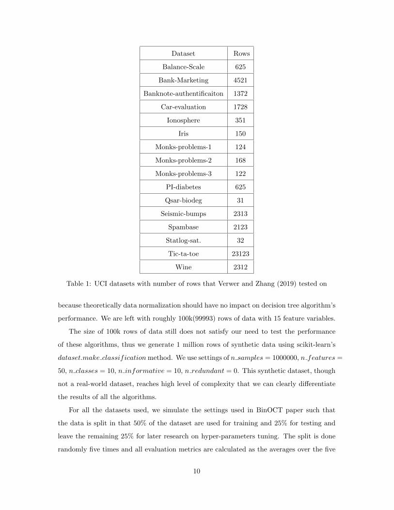
the chosen datasets are rather small in our consideration as the following Table shows their

number of rows of data entries.

Most of the datasets are only a few hundred rows. In modern real applications data

can to go as much as millions, so we test it out on real-world datasets with far more rows

to see if the algorithm still performs well.

We use Rain in Australia dataset 1 which is a real-world dataset offered on Kaggle

data science community. It contains 10 years of daily weather observations from numerous

Australian weather stations of labels as Yes or No to represent if the next day rains or not.

Feature variables are information of min/max temperatures, wind flows, etc. Sample rows

are as follows (not all feature column are included due to space limit):

Figure 2: sample Rain in Australia dataset rows

We preprocess the data in the following steps: we remove the columns that contain

too many empty entries and also remove location and date columns which are not helpful

or hard to convert to numerical values. Then we convert the wind directions to classes of

values from 1 to 16, and Yes and No to 1 and 0 respectively. Normalization is not done

1https://www.kaggle.com/jsphyg/weather-dataset-rattle-package

9

Dataset Rows

Balance-Scale 625

Bank-Marketing 4521

Banknote-authentificaiton 1372

Car-evaluation 1728

Ionosphere 351

Iris 150

Monks-problems-1 124

Monks-problems-2 168

Monks-problems-3 122

PI-diabetes 625

Qsar-biodeg 31

Seismic-bumps 2313

Spambase 2123

Statlog-sat. 32

Tic-ta-toe 23123

Wine 2312

Table 1: UCI datasets with number of rows that Verwer and Zhang (2019) tested on

because theoretically data normalization should have no impact on decision tree algorithm’s

performance. We are left with roughly 100k(99993) rows of data with 15 feature variables.

The size of 100k rows of data still does not satisfy our need to test the performance

of these algorithms, thus we generate 1 million rows of synthetic data using scikit-learn’s

dataset.make classification method. We use settings of n samples = 1000000, n features =

50, n classes = 10, n informative = 10, n redundant = 0. This synthetic dataset, though

not a real-world dataset, reaches high level of complexity that we can clearly differentiate

the results of all the algorithms.

For all the datasets used, we simulate the settings used in BinOCT paper such that

the data is split in that 50% of the dataset are used for training and 25% for testing and

leave the remaining 25% for later research on hyper-parameters tuning. The split is done

randomly five times and all evaluation metrics are calculated as the averages over the five

10

trials. We learn trees of depth 4 in order to match the performance scores reported by the

BinOCT paper.

We then run the BinOCT and CART algorithms on our training set and test its perfor-

mance and ability to generalize on our test set. All training and testing is done on macOS

Catalina version 10.15.1 with 3.1 GHz Dual-Core Intel Core i7 CPU. The reason we choose

not to run the training on a GPU which is more common to machine learning applications

is because we want to test out and compare the running time of the algorithms while on

GPU the training finishes too fast within seconds for smaller datasets such that it would

be harder to tell the difference.

3.3 Result

We care more about the performance of the algorithms on large datasets. The results of

BinOCT and CART algorithms on Rain in Australia dataset and the 1 million row synthetic

dataset are as follows.

We show a more specific score evaluation of CART algorithm on Rain in Australia

dataset in Table 2, but we use classification accuracy scores on test set as the main evalu-

ation metric later on.

Class Precision Recall F1-score

0 0.86 0.95 0.90

1 0.73 0.46 0.56

Table 2: CART algorithm performance scores on Rain in Australia dataset in a randomly

split 50% training set 25% test set run

With 5 runs, the average classification accuracy of CART algorithm on Rain in Australia

is 83.58%, while BinOCT algorithm reaches 84.15%. The difference is surprisingly small.

Additional runs demonstrate that BinOCT does perform a bit better than CART in terms

of classification accuracy when reproducing and confirming the results on smaller UCI

datasets that Verwer and Zhang (2019) tested on. BinOCT also does run a little bit faster

than CART, but this should not be considered a valid conclusion because when training on

small scale data, overhead matters much more than algorithm complexity.

Then as we test the running time of algorithms on the Rain in Australia dataset,

11

BinOCT algorithm uses roughly 2 seconds compared to CART using 1 second on Rain

in Australia. It might be considered minimal difference here which is why we adopt the

synthetic dataset to enlarge the difference. With the 1 million rows synthetic dataset we cre-

ate, there are 50 feature variables and 10 classes which make the classification much harder.

It takes BinOCT roughly 20 minutes to reach 30.89% classification accuracy, and CART

roughly 2 minutes to reach 30.87%. The result scores are almost identical but BinOCT

does not run faster than CART algortihm as the authors claim it to excel on. This could

be due to code implementation not being optimized, which requires further research. More

results can be found in the next part.

3.4 Comparison to Methods taught in Class

Since this is a course project, we are interested in how the decision tree algorithms perform

in comparison to algorithms taught in class that are highly related: logistic regression and

random forests. We implement these algorithms and show the accuracy score as main

metric below on all the datasets we have.

We present the accuracy scores on test set on seventeen datasets including mostly small

UCI datasets and large ones of Rain in Australia and our synthetic dataset. From Table

3, we can see that all four algorithms work better on smaller datasets with fewer features.

Logistic Regression algorithm seems to be a more stable one which performs well on all the

datasets used.

4 Conclusion

From the results of our experiments including the table given above, it is still hard to

generalize a straightforward conclusion on which algorithm is the best overall algorithm.

As on different datasets the winning algorithm is different. This is inspiring result as simple

algorithms as decision trees that are easy to implement and understand can also reach high

performances. It has the advantage that less pre-processing on data needs to be done,

but also the disadvantage that training is considerably slower with more data and feature

variables added.

If we simply judge from the number of cases with highest classification accuracy, logistic

12

Dataset CART BinOCT Logistic Regression Random Forest # Feature

Balance-Scale 67.5 69.3 88.8 85.1 4

Bank-Marketing 88.9 90.3 90.1 88.7 17

Banknote-authentificaiton 90.6 91.7 99.0 96.6 4

Car-evaluation 77.8 77.8 80.0 80.1 5

Ionosphere 87.8 87.7 86.6 89.6 34

Iris 95.8 96.3 84.7 91.6 4

Monks-problems-1 68.4 80.0 66.5 78.1 6

Monks-problems-2 60.9 58.1 61.4 60.0 6

Monks-problems-3 94.2 93.5 77.4 88.4 6

PI-diabetes 74.7 75.4 77.4 76.0 8

Qsar-biodeg 76.8 78.6 85.4 83.8 41

Spambase 85.4 85.7 92.6 91.2 57

Statlog-sat. 63.4 67.5 92.5 99.7 36

Tic-ta-toe 68.5 67.3 96.4 80.8 18

Wine 88.0 91.1 92.4 95.1 13

Rain in Australia 83.6 84.1 84.6 83.7 15

Synthetic(1 million) 30.87 30.89 39.5 40.6 50

Table 3: Comparison of average classification accuracy scores on test set of 4 algorithms on

UCI dataset, Rain in Australia dataset and our synthetic dataset

regression will be ”the best”. There are eight out of seventeen datasets where logistic re-

gression has the highest classification accuracy. It outcompetes decision trees and random

forests when there are fewer numbers of features. But as the feature number increases, lo-

gistic regression somehow presents similar or less accuracy compared with CART, BinOCT,

and Random Forests.

While our experiment results disagree with Verwer and Zahng (2019) concerning the

comparison between BinOCT and CART, it is possible that our procedure of reproducing

their results has undetected limitations leading to such disagreement. Otherwise it is ques-

tionable if BinOCT significantly improves classification accuracy within shorter running

time on both small and large problems as expected. Moreover, while the formulation of

13

BinOCT reduces encoding constraints and variables, it is unclear to us if BinOCT captures

the underlying nature of training data better than CART does even though the authors of

BinOCT point out the greedy nature of CART.

5 Future Works

We admit that there are many steps and processes in our experiments that could be ame-

liorated. If further time is given for the project, we plan to work on the following aspects

to perfect our research.

1. Hyper-parameters tuning. This is likely the most important aspect that we are not

fully exploring on because of time and resource limit. There are tons of hyper-parameters

in the algorithms we have not explored, especially tree depth of the decision tree algorithms

and its effect on the overall performances of the algorithms.

2. More real-world datasets. The performance of the BinOCT algorithm on large-scale

dataset remains questionable after our experiments and careful evaluation on the results.

More testing on larger dataset of different feature variable number and classes number

would be preferable to reach a conclusion on the algorithm.

Author’s Contributions

Siyang Li, Shaoshan Zeng, and Jiawen Wu conceptualized the research project. Siyang Li

and Shaoshan Zeng formulated and implemented the algorithm, generated initial simulated

data and performed the analysis of simulated and real data. Siyang Li designed the extended

simulation study and performed the extended simulation study on BinOCT and other

existing methods. Jiawen Wu and Shaoshan Zeng bring introdution to the general topic

and lead to a comparison of different methods. Siyang Li processed and contributed in the

analysis of real data. Siyang Li, Shaoshan Zeng, and Jiawen Wu prepared the initial draft

of the manuscript and contributed in preparing the final version of the manuscript. All

authors read and approved the final manuscript.

14

Appendix

Our code:

Figure 3: Code sample

Figure 4: Recursive algorithm provided by Verwer and Zhang (2019), where th(i) returns

the ith threshold value.

15

ReferencesBertsimas, D. and J. Dunn (2017). Optimal classification trees. Machine Learning 106.7

(2017): 1039–1082 .

Breiman, L. (1984). Classification and Regression Trees. Belmont, CA: Wadsworth Inter-national Group.

Breiman, L. (2001). Random forests. Machine Learning 45, 5–32. Available at https:

//doi.org/10.1023/A:1010933404324.

Breunig, M. M., H.-P. Kriegel, R. T. Ng, and J. Sander (2000). LOF: Identifying density-based local outliers. In Proceedings of the 2000 ACM SIGMOD International Conferenceon Management of Data, pp. 93–104. ACM.

Esmeir, S. and S. Markovitch (2007). Anytime learning of decision trees. The Journal ofMachine Learning Research 8, 891–933.

Hastie, T., R. Tibshirani, and J. Friedman (2009). The Elements of Statistical Learning:Data Mining, Inference, and Prediction (2nd ed.). New York, NY: Springer.

Kelley, N. D. and B. J. Jonkman (2003). Overview of the TurbSim stochastic inflowturbulence simulator. NREL/TP-500-41137, Version 1.21, National Renewable EnergyLaboratory, Golden, Colorado. Available at https://nwtc.nrel.gov/system/files/

TurbSimOverview.pdf.

Norton, S. W. (1989). Generating better decision trees. In IJCAI.

Quinlan, J. R. (1986). Induction of decision trees. Mach Learn 1, 81–106. Available athttps://doi.org/10.1007/BF00116251.

Salzberg, S. L. (1993). Programs for machine learning by j. ross quinlan. morgan kaufmannpublishers, inc., 1993. Mach Learn 16, 235–240. Available at https://doi.org/10.

1007/BF00993309.

Verwer, S. and Y. Zhang (2019). Learning optimal classification trees using a binary linearprogram formulation. Proceedings of the AAAI Conference on Artificial Intelligence,33(01), 1625-1632..

William, J. L., L. G. John, P. S. Harry, and B. D. Ralph (1993). A comparison of logisticregression to decision-tree induction in a medical domain. Computers and BiomedicalResearch 26, 74–97. Available at https://doi.org/10.1006/cbmr.1993.1005.

Yang, J. and T. S. Huang (2010). Image super-resolution: Historical overview and futurechallenges. In P. Milanfar (Ed.), Super-Resolution Imaging, pp. 3–35. Boca Raton, FL:Chapman & Hall/CRC Press.

16