the tridas project - infn-bo · our daily work has received precious help from shamaila ahmad,...
TRANSCRIPT

CMSThe TriDAS Project
Technical Design Report, Volume 2:
Data Acquisition and High-Level TriggerAlso available at http://cmsdoc.cern.ch/cms/TDR/DAQ/daq.html
CMS TriDAS project
Chairperson Institution Board: Paris Sphicas, CERN, MIT and University of Athens, [email protected]
Trigger/DAQ Project Manager Trigger Project Manager DAQ Project Manager
Sergio Cittolin, [email protected]
Wesley Smith, University of [email protected]
Sergio Cittolin, [email protected]
Trigger/DAQ Resource Manager Trigger Technical Coordinator DAQ Technical Coordinator
Joao Varela, LIP/[email protected]
Attila Racz, [email protected]
CMS Spokesperson CMS Technical Coordinator
Michel Della Negra, [email protected]
Alain Herve, [email protected]
CERN/LHCC 02-26CMS TDR 6
December 15, 2002

CMS: The Trigger/DAQ project Technical Design ReportData Acquisition and High-Level Trigger CERN / LHCC 02-26
ii

CMS: The Trigger/DAQ project Technical Design ReportData Acquisition and High-Level Trigger CERN / LHCC 02-26
Editor
P. Sphicas
Chapter Editors
D. Acosta, J. Branson, S. Cittolin, A. De Roeck, S. Eno, S. Erhan, F. Glege, J. Gutleber, G. Maron,F. Meijers, E. Meschi, S. Murray, A. Oh, L. Orsini, V. O’Dell, A. Racz, P. Scharff-Hansen, C. Schwick,C. Seez, L. Silvestris, K. Sumorok.
Cover Design
S. Cittolin
Acknowledgements
The CMS Data Acquisition community wishes to thank all the people who have contributed to the workpresented in this Technical Design Report.
We would like to thank our CMS internal reviewers C. Foudas, R. Clare and H. von der Schmidt, for alltheir help, constructive comments and suggestions. We would also like to thank our LHCC refereesS. Bertolucci, J. Nash, K. Tokushuku and C. Vallee, who have followed the project in the past severalyears and have offered us plenty of support.
Our daily work has received precious help from Shamaila Ahmad, Kirsti Aspola, Madeleine Azeglio,Nadejda Bogolioubova, Dawn Hudson, Delphine Labrousse, Anne Lissajoux, Guy Martin and Marie-Claude Pelloux.
The Spring02 production would not have been successful without the effort of a large team of people run-ning and supporting the production in various ways. We wish to thank in particular the following people:S. Aziz, C. Charlot, D. Colling, M Ernst, A. Filine, R. Gowrishankara, N. Kruglov, A. Kryukov, J. Letts,P. Lewis, C. Mackay, P. Mine, S. Muzaffar, S. Singh, E. Tikhonenko, Y. Wu.
We also wish to thank our collaborators on CMS, and especially the CMS management, for their supportand encouragement.
iii

CMS: The Trigger/DAQ project Technical Design ReportData Acquisition and High-Level Trigger CERN / LHCC 02-26
iv

CMS: The Trigger/DAQ project Data Acquisition and High-Level TriggerTechnical Design Report, Volume II CMS Collaboration
CMS Collaboration
Yerevan Physics Institute, Yerevan, ARMENIAG.L. Bayatian, N. Grigorian, V.G. Khachatrian, A. Margarian, A.M. Sirunyan, S. Stepanian
Institut für Hochenergiephysik der OeAW, Wien, AUSTRIAW. Adam, T. Bauer, T. Bergauer, J. Erö, M. Friedl, R. Fruehwirth, J. Hrubec, A. Jeitler, M. Krammer, N. Neumeister1, M. Pernicka, P. Porth, H. Rohringer, H. Sakulin, J. Strauss, A. Taurok, W. Waltenberger, G. Walzel, C.-E. Wulz
Research Institute for Nuclear Problems, Minsk, BELARUSA. Fedorov, N. Gorodichenine, M. Korzhik, V. Panov, V. Yeudakimau, R. Zuyeuski
National Centre for Particle and High Energy Physics, Minsk, BELARUSV. Chekhovsky, I. Emeliantchik, M. Kryvamaz, A. Litomin, V. Mossolov, S. Reutovich, N. Shumeiko, A. Solin, A. Tikhonov, V. Zalessky
Byelorussian State University, Minsk, BELARUSV. Petrov
Vrije Universiteit Brussel, Brussel, BELGIUMO. Devroede, R. Goorens, J. Lemonne, S. Lowette, S. Tavernier, B. Van De Vyver1, W. Van Doninck1, L. Van Lancker, C. Yu
Université Libre de Bruxelles, Bruxelles, BELGIUMO. Bouhali, B. Clerbaux, G. De Lentdecker, P. Marage, C. Vander Velde, P. Vanlaer, J. Wickens
Université Catholique de Louvain, Louvain-la-Neuve, BELGIUMS. Assouak, J.L. Bonnet, E. Burton, B. De Callatay, J. De Favereau De Jeneret, G. De Hemptinne, C. Delaere, T. Delbar, D. Favart, E. Forton, J. Govaerts, G. Grégoire, G. Leibenguth, V. Lemaitre, Y. Longree, D. Michotte, O. Militaru, A. Ninane, F. Payen, K. Piotrzkowski, X. Rouby, O. van der Aa
Université de Mons-Hainaut, Mons, BELGIUMI. Boulogne, E. Daubie, P. Herquet
Universitaire Instelling Antwerpen, Wilrijk, BELGIUMW. Beaumont, T. Beckers, E. De Langhe, E. De Wolf, F. Moortgat, F. Verbeure
Institute for Nuclear Research and Nuclear Energy, Sofia, BULGARIAK. Abadjiev, T. Anguelov, I. Atanasov, J. Damgov, L. Dimitrov, V. Genchev, P. Iaydjiev, B. Kounov, P. Petkov, S. Piperov, G. Sultanov, I. Vankov
University of Sofia, Sofia, BULGARIAA. Dimitrov, I. Glushkov, L. Litov, M. Makariev, M. Mateev, I. Nasteva, B. Pavlov, P. Petev, S. Stoynev, V. Velev
Institute of High Energy Physics, Beijing, CHINA, PRJ. Bai, J.G. Bian, G.M. Chen, H.S. Chen, Y.N. Guo, K. He, G. Huang, C.H. Jiang, Z.J. Ke, J. Li, W.G. Li, H. Liu, J.F. Qiu, X. Shen, Y.Y. Wang, M. Yang, B.Y. Zhang, S.Q. Zhang, W. Zhao, Z.G. Zhao, L. Zhou, G.Y. Zhu, Z. Zhu
Peking University, Beijing, CHINA, PRY. Ban, J. Cai, H.T. Liu, Y.L. Ye, J. Ying
University for Science and Technology of China, Hefei, Anhui, CHINA, PRZ.P. Zhang, J. Zhao
Shanghai Institute of Ceramics, Shanghai, CHINA, PR (associated institute)Q. Deng, P.J. Li, D.Z. Shen, Z.L. Xue, P. Yang1, H. Yuan
National Central University, Chung-Li, CHINA (TAIWAN)Y.H. Chang, E.A. Chen, A. Go, W. Lin
v

CMS: The Trigger/DAQ project Data Acquisition and High-Level TriggerTechnical Design Report, Volume II CMS Collaboration
National Taiwan University (NTU), Taipei, CHINA (TAIWAN)S. Blyth, P. Chang, Y. Chao, K.F. Chen, Z. Gao1, G.W.S. Hou, H.C. Huang, K. Ueno, Y. Velikzhanin, M. Wang, P. Yeh
Technical University of Split, Split, CROATIAN. Godinovic, I. Puljak, I. Soric
University of Split, Split, CROATIAZ. Antunovic, M. Dzelalija, K. Marasovic
University of Cyprus, Nicosia, CYPRUSP. Demetriou, C. Nicolaou, P.A. Razis, D. Tsiakkouri
National Institute of Chemical Physics and Biophysics, Tallinn, ESTONIAE. Lippmaa, M. Raidal1, J. Subbi
Laboratory of Advanced Energy Systems, Helsinki University of Technology, Espoo, FINLANDP.A. Aarnio
Helsinki Institute of Physics, Helsinki, FINLANDK. Banzuzi, S. Czellar1, P.O. Friman1, J. Härkönen, M.A. Heikkinen, J.V. Heinonen, V. Karimäki, H.M. Katajisto, R. Kinnunen, T. Lampén, K. Lassila-Perini, V. Lefébure1, S. Lehti, T. Lindén, P.R. Luukka, S. Nummela, E. Tuominen, J. Tuominiemi, D. Ungaro
Dept. of Physics & Microelectronics Instrumentation Lab., University of Oulu, Oulu, FINLANDT. Tuuva
Digital and Computer Systems Laboratory, Tampere University of Technology, Tampere, FINLANDJ. Niittylahti
Laboratoire d’Annecy-le-Vieux de Physique des Particules, IN2P3-CNRS, Annecy-le-Vieux, FRANCEJ.P. Guillaud, M. Maire, J.P. Mendiburu, P. Nedelec, J.P. Peigneux, M. Schneegans, D. Sillou
DSM/DAPNIA, CEA/Saclay, Gif-sur-Yvette, FRANCEM. Anfreville, C. Bouchand, P. Bredy, R. Chipaux, M. Dejardin1, D. Denegri, B. Fabbro, J.L. Faure, F.X. Gentit, A. Givernaud, P. Jarry, F. Kircher, T. Lasserre, M.C. Lemaire, Y. Lemoigne, B. Levesy, E. Locci, J.P. Lottin, M. Mur, E. Pasquetto, A. Payn, J. Rander, J.M. Reymond, F. Rondeaux, A. Rosowsky, A. Van Lysebetten, P. Verrecchia
Laboratoire Leprince-Ringuet, Ecole Polytechnique, IN2P3-CNRS, Palaiseau, FRANCEM. Bercher, J. Bourotte1, P. Busson, D. Chamont, C. Charlot, C. Collard, L. Dobrzynski, Y. Geerebaert, J. Gilly, M. Haguenauer, A. Karar, D. Lecouturier, G. Milleret, P. Miné, R. Morano, P. Paganini, P. Poilleux, N. Regnault, T. Romanteau, I. Semeniouk
Institut de Recherches Subatomiques, IN2P3-CNRS - ULP, LEPSI Strasbourg, UHA Mulhouse, Stras-bourg, FRANCEJ.D. Berst2, R. Blaes3, D. Bloch, J.M. Brom, F. Charles3, G.L. Claus, J. Coffin, F. Didierjean, F. Drouhin3, J.P. Ernenwein3, J.C. Fontaine3, U. Goerlach, P. Graehling, L. Gross, D. Huss, C. Illinger2, P. Juillot, A. Lounis, C. Maazouzi, S. Moreau, I. Ripp-Baudot, R. Strub, T. Todorov, P. Van Hove, D. Vintache
Institut de Physique Nucléaire de Lyon, IN2P3-CNRS, Univ. Lyon I, Villeurbanne, FRANCEM. Ageron, M. Bedjidian, A. Bonnevaux, E. Chabanat, C. Combaret, D. Contardo, R. Della Negra, P. Depasse, M. Dupanloup, T. Dupasquier, H. El Mamouni, N. Estre, J. Fay, S. Gascon, N. Giraud, C. Girerd, R. Haroutounian, J.C. Ianigro, B. Ille, M. Lethuillier, N. Lumb, L. Mirabito1, S. Perries, O. Ravat, B. Trocme
High Energy Physics Institute, Tbilisi State University, Tbilisi, GEORGIAR. Kvatadze, D. Mzavia
Institute of Physics Academy of Science, Tbilisi, GEORGIAV. Roinishvili
RWTH, I. Physikalisches Institut, Aachen, GERMANYR. Adolphi, W. Braunschweig, H. Esser, A. Heister, W. Karpinski, S. König, C. Kukulies, J. Olzem,
vi

CMS: The Trigger/DAQ project Data Acquisition and High-Level TriggerTechnical Design Report, Volume II CMS Collaboration
A. Ostaptchouk, D. Pandoulas, G. Pierschel, F. Raupach, S. Schael, A. Schultz von Dratzig, B. Schwering, G. Schwering, R. Siedling, B. Wittmer, M. Wlochal
RWTH, III. Physikalisches Institut A, Aachen, GERMANYA. Adolf, C. Autermann, A. Böhm, M. Bontenackels, H. Fesefeldt, T. Hebbeker, S. Hermann, G. Hilgers, K. Hoepfner, D. Lanske, B. Philipps, D. Rein, H. Reithler, M. Sowa, T. Stapelberg, H. Szczesny, M. Tonutti, O. Tsigenov, M. Wegner
RWTH, III. Physikalisches Institut B, Aachen, GERMANYM. Axer, F. Beissel, V. Commichau, G. Flügge, T. Franke, K. Hangarter, T. Kress, J. Mnich, A. Nowack, M. Poettgens, O. Pooth, P. Schmitz, M. Weber
Institut für Experimentelle Kernphysik, Karlsruhe, GERMANYV. Bartsch, P. Blüm, W. De Boer, A. Dierlamm, G. Dirkes, M. Erdmann, M. Fahrer, M. Feindt, A. Furgeri, P. Gras, E. Grigoriev, F. Hartmann, S. Heier, J. Kaminski, S. Kappler, T. Müller, C. Piasecki, G. Quast, K. Rabbertz, H.J. Simonis, A. Skiba, A. Theel, T. Weiler, C. Weiser, V. Zhukov4
University of Athens, Athens, GREECEA. Angelis, G. Daskalakis, A. Panagiotou1
Institute of Nuclear Physics "Demokritos", Attiki, GREECEM. Barone, T. Geralis, C. Kalfas, D. Loukas, A. Markou, C. Markou, K. Zachariadou
University of Ioánnina, Ioánnina, GREECEA. Asimidis, X. Aslanoglou, I. Evangelou, P. Kokkas, N. Manthos, G. Sidiropoulos, F.A. Triantis, P. Vichoudis
KFKI Research Institute for Particle and Nuclear Physics, Budapest, HUNGARYG. Bencze, L. Boldizsar, P. Hidas, G. Odor, G. Vesztergombi, P. Zalan
Institute of Nuclear Research ATOMKI, Debrecen, HUNGARYJ. Molnar
Kossuth Lajos University, Debrecen, HUNGARYG. Marian, P. Raics, Z. Szabo, Z. Szillasi, G. Zilizi
Panjab University, Chandigarh, INDIAS.B. Beri, V. Bhatnagar, M. Kaur, J.M. Kohli, J. Singh
University of Delhi, Delhi, INDIAA. Bhardwaj, S. Chatterji, K. Ranjan, R.K. Shivpuri
Bhabha Atomic Research Centre, Mumbai, INDIAS. Borkar, M. Dixit, M. Ghodgaonkar, S.K. Kataria, S.K. Lalwani1, V. Mishra, A. Topkar
Tata Institute of Fundamental Research - EHEP, Mumbai, INDIAT. Aziz, S. Banerjee, S. Chendvankar, P.V. Deshpande, A. Gurtu, G. Majumder, K. Mazumdar1, M.R. Patil, K. Sudhakar, S.C. Tonwar
Tata Institute of Fundamental Research - HECR, Mumbai, INDIAB.S. Acharya, S. Banerjee, S. Bheesette, S. Dugad, S.D. Kalmani, V.R. Lakkireddi, N.K. Mondal, N. Panyam, P. Verma
Institute for Studies in Theoretical Physics & Mathematics (IPM), Tehran, IRANF. Ardalan, H. Arfaei, R. Mansouri, M. Mohammadi
Università di Bari, Politecnico di Bari e Sezione dell' INFN, Bari, ITALYM. Abbrescia, E. Carrone1, E. Cavallo, A. Colaleo, D. Creanza, N. De Filippis, M. De Palma, L. Fiore, D. Giordano, G. Iaselli, F. Loddo, G. Maggi, M. Maggi, B. Marangelli, S. My, S. Natali, S. Nuzzo, G. Pugliese, V. Radicci, A. Ranieri, F. Romano, F. Ruggieri, G. Selvaggi, L. Silvestris, P. Tempesta, R. Trentadue, P. Vankov, G. Zito
Università di Bologna e Sezione dell' INFN, Bologna, ITALYS. Arcelli, A. Benvenuti, D. Bonacorsi, P. Capiluppi, F. Cavallo, M. Cuffiani, I. D’Antone, G.M. Dallavalle, F. Fabbri, A. Fanfani, P. Giacomelli5, C. Grandi, M. Guerzoni, S. Marcellini, P. Mazzanti, A. Montanari,
vii

CMS: The Trigger/DAQ project Data Acquisition and High-Level TriggerTechnical Design Report, Volume II CMS Collaboration
C. Montanari, F. Navarria, F. Odorici, A. Perrotta, A. Rossi, T. Rovelli, G. Siroli, R. Travaglini
Università di Catania e Sezione dell' INFN, Catania, ITALYS. Albergo, V. Bellini, S. Cavalieri, M. Chiorboli, S. Costa, R. Potenza, C. Randieri, C. Sutera, A. Tricomi, C. Tuve
Università di Firenze e Sezione dell' INFN, Firenze, ITALYA. Bocci, E. Borchi, V. Ciulli, C. Civinini, R. D’Alessandro, E. Focardi, A. Macchiolo, N. Magini, C. Marchettini, M. Meschini, S. Paoletti, G. Parrini, R. Ranieri, M. Sani
Università di Genova e Sezione dell' INFN, Genova, ITALYP. Fabbricatore, M. Fossa, R. Musenich, C. Pisoni
Laboratori Nazionali di Legnaro dell' INFN, Legnaro, ITALY (associated institute)L. Berti, M. Biasotto, E. Ferro, U. Gastaldi, M. Gulmini1, G. Maron, N. Toniolo, L. Zangrando
Istituto Nazionale di Fisica Nucleare e Universita Degli Studi Milano-Bicocca, Milano, ITALYM. Bonesini, G. Franzoni, A. Ghezzi, P. Govoni, A. Meregaglia, P. Negri, M. Paganoni, A. Pullia, S. Ragazzi, N. Redaelli, T. Tabarelli de Fatis
Istituto Nazionale di Fisica Nucleare de Napoli (INFN), Napoli, ITALYL. Lista, P. Paolucci, D. Piccolo
Università di Padova e Sezione dell' INFN, Padova, ITALYM. Bellato, M. Benettoni, D. Bisello, A. Candelori, P. Checchia, E. Conti, M. Corvo, M. De Giorgi, A. De Min, U. Dosselli, C. Fanin, F. Fanzago, F. Gasparini, U. Gasparini, F. Gonella, A. Kaminski, S. Lacaprara, I. Lippi, M. Loreti, O. Lytovchenko, M. Mazzucato, A.T. Meneguzzo, M. Michelotto, F. Montecassiano1, M. Nigro, M. Passaseo, M. Pegoraro, P. Ronchese, E. Torassa, S. Vanini, L. Ventura, S. Ventura, M. Zanetti, P. Zotto, G. Zumerle
Università di Pavia e Sezione dell' INFN, Pavia, ITALYG. Belli, R. Guida, S.P. Ratti, P. Torre, P. Vitulo
Università di Perugia e Sezione dell' INFN, Perugia, ITALYM.M. Angarano, E. Babucci, M. Biasini, G.M. Bilei1, M.T. Brunetti, B. Checcucci, N. Dinu, L. Fanò, M. Giorgi, P. Lariccia, G. Mantovani, D. Passeri, P. Placidi, V. Postolache, D. Ricci, M. Risoldi, R. Santinelli, A. Santocchia, L. Servoli
Università di Pisa, Scuola Normale Superiore e Sezione dell' INFN, Pisa, ITALYG. Bagliesi, A. Bardi, A. Basti, J. Bernardini, T. Boccali, L. Borrello, F. Bosi, P.L. Braccini, R. Castaldi, R. Cecchi, R. Dell'Orso, S. Donati, F. Donno, S. Dutta, L. Foà, S. Galeotti, S. Gennai, A. Giassi, S. Giusti, G. Iannaccone, A. Kyriakis, L. Latronico, F. Ligabue, M. Massa, A. Messineo, A. Moggi, F. Morsani, F. Palla, F. Palmonari, F. Raffaelli, G. Sanguinetti, G. Segneri, P. Spagnolo, M. Spezziga, F. Spinella, A. Starodumov6, G. Tonelli, C. Vannini, P.G. Verdini, J.C. Wang
Università di Roma I e Sezione dell' INFN, Roma, ITALYS. Baccaro7, L. Barone, A. Bartoloni, F. Cavallari, S. Costantini, I. Dafinei, M. Diemoz, C. Gargiulo, E. Longo, P. Meridiani, M. Montecchi7, G. Organtini, R. Paramatti
Università di Torino e Sezione dell' INFN, Torino, ITALYN. Amapane, M. Arneodo, F. Bertolino, C. Biino1, R. Cirio, M. Costa, D. Dattola1, L. Demaria, G. Favro, S. Maselli, E. Migliore, V. Monaco, C. Peroni, A. Romero, M. Ruspa, R. Sacchi, A. Solano, A. Staiano, P.P. Trapani
Chungbuk National University, Chongju, KOREAY.U. Kim
Kangwon National University, Chunchon, KOREAS.K. Nam
Wonkwang University, Iksan, KOREAS.Y. Bahk
viii

CMS: The Trigger/DAQ project Data Acquisition and High-Level TriggerTechnical Design Report, Volume II CMS Collaboration
Cheju National University, Jeju, KOREAY.J. Kim
Chonnam National University, Kwangju, KOREAJ.Y. Kim, I.T. Lim
Dongshin University, Naju, KOREAM.Y. Pac
Seonam University, Namwon, KOREAS.J. Lee
Konkuk University, Seoul, KOREAS.Y. Jung, J.T. Rhee
Korea University, Seoul, KOREAB.S. Hong, S.J. Hong, K.S. Lee, S.K. Park, K.S. Sim
Seoul National University of Education, Seoul, KOREAD.G. Koo
Seoul National University, Seoul, KOREAK.K. Joo, B.J. Kim, S.B. Kim, I.H. Park
Sungkyunkwan University, Suwon, KOREAB.G. Cheon, Y.I. Choi
Kyungpook National University, Taegu, KOREAK. Cho, S.W. Ham, D.H. Kim, G.N. Kim, W.Y. Kim, J.Y. Lee, S.K. Oh, Y.D. Oh, S.R. Ro, D.C. Son
National Centre for Physics, Quaid-I-Azam University, Islamabad, PAKISTANZ. Aftab, M. Ahmad, I. Ahmed, M.I. Asghar, H.R. Hoorani, S.M. Khan, A. Osman1, N. Qaiser, R. Riazuddin, T. Solaija
National University of Sciences And Technology, Rawalpindi Cantt, PAKISTAN (associated institute)A. Ali, A. Bashir, A. Muhammad, M. Saeed
Institute of Experimental Physics, Warsaw, POLANDM. Bluj, K. Bunkowski, M. Cwiok, H. Czyrkowski, R. Dabrowski, W. Dominik, K. Doroba, M. Kazana, J. Krolikowski, I. Kudla, M. Pietrusinski, K. Pozniak22, W. Zabolotny22, J. Zalipska, P. Zych
Soltan Institute for Nuclear Studies, Warsaw, POLANDM. Górski, L. Goscilo, K. Nawrocki, G. Wrochna, P. Zalewski
Laboratório de Instrumentação e Física Experimental de Partículas, Lisboa, PORTUGALR. Alemany-Fernandez, C. Almeida, N. Almeida, J. Augusto, P. Bordalo, S. Da Mota Silva, J. Da Silva, O.P. Dias, J. Gomes, F.M. Goncalves, N. Leonardo, S. Ramos, R. Ribeiro, M. Santos, J. Semiao, I. Teixeira, J.P. Teixeira, J. Varela, N. Vaz Cardoso
Joint Institute for Nuclear Research, Dubna, RUSSIAI. Anissimov, A. Belkov, A. Cheremukhin, A. Dmitriev, V. Elsha, Y. Erchov, I. Golutvin, N. Gorbunov, I. Gramenitsky, A. Janata, V. Kalagin, V. Karjavin, A. Karlov, S. Khabarov, V. Khabarov, Y. Kiryushin, V. Kolesnikov, V. Konoplyanikov, V. Korenkov, I. Kossarev, V. Ladyguine, V. Lysiakov, A. Malakhov, I. Melnichenko, G. Meshcheryakov, V.V. Mitsyn, P. Moisenz, S. Movchan, V. Palichik, V. Perelygin, A. Rogov, S. Sergeev, A. Sergueev, S. Shmatov, S. Shulha, I. Slepnev, V. Smirnov, D. Smolin, E. Tikhonenko, A. Urkinbaev8, E. Vedenyapina, A. Vichnevski, A. Volodko, N. Zamiatin, A. Zarubin, P. Zarubin, E. Zubarev
Petersburg Nuclear Physics Institute, Gatchina (St Petersburg), RUSSIAA. Atamantchouk, A. Baldychev, V. Barashko, N. Bondar, V. Golovtsov, D. Goulevich, Y. Ivanov, V. Kim, E. Kouznetsova, V. Kozlov, E. Lobatchev, G. Makarenkov, E. Orishchin, V. Rasmislovich, B. Razmyslovich, V. Sknar, I. Smirnov, S. Sobolev, I. Tkach, L. Uvarov, G. Velitchko, S. Volkov, A. Vorobyev, D. Yakorev
Institute for Nuclear Research, Moscow, RUSSIAI. Andreev, P. Antipov, G.S. Atoyan, S. Gninenko, N. Goloubev, E.V. Gushin, M. Kirsanov, A. Kovzelev,
ix

CMS: The Trigger/DAQ project Data Acquisition and High-Level TriggerTechnical Design Report, Volume II CMS Collaboration
N. Krasnikov, V. Matveev, A. Pashenkov, A. Poliarouch, V.E. Postoev, V. Shmatkov, A. Skassyrskaia9, A. Solovey, L. Stepanova, A. Toropin9
Institute for Theoretical and Experimental Physics, Moscow, RUSSIAV. Gavrilov, N. Ilina, V. Kaftanov, I. Kisselevitch, V. Kolosov, M. Kossov, A. Krokhotine, S. Kuleshov, N. Stepanov, V. Stoline, S. Uzunyan, V. Zakharov
P.N. Lebedev Physical Institute, Moscow, RUSSIAA.M. Fomenko, N. Konovalova, V. Kozlov, A.I. Lebedev, N. Lvova, S. Potashov, S.V. Rusakov
Moscow State University, Moscow, RUSSIAE. Boos, A. Cherstnev, L. Dudko, A. Erchov, R. Gloukhov, A. Gribushin, V. Ilyin, O.L. Kodolova1, A. Kryukov, I.P. Lokhtin, V. Mikhaylin, L. Sarycheva, V. Savrin, L. Shamardin, A. Snigirev, I. Vardanyan
High Temperature Technology Center of Research & Development Institute of Power Engineering (HTTC RDIPE), Moscow, RUSSIA (associated institute)D. Chmelev, D. Druzhkin, A. Ivanov, V. Koudinov, O. Logatchev, S. Onishchenko, A. Orlov, V. Sakharov, V. Smetannikov, A. Tikhomirov, S. Zavodthikov
State Research Center of Russian Federation - Institute for High Energy Physics, Protvino, RUSSIAA. Abramov, V. Abramov, A. Annenkov10, I. Azhgirey, S. Belyanchenko, S. Bitioukov, P. Goncharov, V. Goussev, V. Grichine, A. Inyakin, V. Katchanov, A. Khmelnikov, E. Kolatcheva, A. Korablev, Y. Korneev, A. Kostritski, A. Krinitsyn, V. Kryshkin, E. Kvachina, O. Lapyguina, A. Levine, A. Markov, V. Medvedev, M. Oukhanov, V. Pak, V. Petrov, V. Pikalov, P. Podlesnyy, V. Potapov, A. Riabov, A. Sannikov, Z. Simonova, E. Skvortsova, S. Slabospitski, A. Sobol, A. Soldatov, S. Stepouchkine, A. Surkov1, A. Sytin, V. Talanov, B. Tchuiko, S. Tereschenko, S. Troshin, L. Turchanovich, N. Tyurin, A. Uzunian, A. Volkov, A. Zaitchenko, S. Zelepoukine
Russian Federal Nuclear Centre - Scientific Research Institute for Technical Physics (RFNC-VNIITF), Snezhinsk, RUSSIA (associated institute)A. Andriyash, D. Batin, D. Gorchkov, D. Griaznykh, O. Gueinak, D. Korotchine, S. Koshelev, S. Kotegov, Y. Kretinin, A. Maloiaroslavtsev, M. Naoumenko, I. Pavlov, V. Pravilnikov, S. Samarine, D. Shadrin, R. Skripov
Electron National Research Institute, St Petersburg, RUSSIA (associated institute)V. Lukyanov, G. Mamaeva, Z. Prilutskaya, I. Rumyantsev, E. Sidorovitch, S. Sokha, S. Tataurschikov, I. Vasilyev
Myasishchev Design Bureau, Zhukovsky, RUSSIA (associated institute)V. Shirinyants
Vinca Institute of Nuclear Sciences, Belgrade, SERBIAP. Adzic, I. Anicin, S. Drndarevic, J. Ilic, D. Krpic, P. Milenovic, J. Puzovic, G. Skoro, N. Smiljkovic, M. Zupan
Slovak University of Technology, Bratislava, SLOVAK REPUBLICK. Vitazek
Centro de Investigaciones Energeticas Medioambientales y Tecnologicas, Madrid, SPAINM. Aguilar-Benitez, J. Alberdi, P. Arce1, C. Burgos, M. Cerrada, N. Colino, M. Daniel, B. De La Cruz, C. Fernandez Bedoya, A. Ferrando, M.C. Fouz, P. Garcia-Abia, M.I. Josa, J.M. Luque, J. Marin, A. Molinero, J.C. Oller, J. Puerta Pelayo, L. Romero, J. Salicio, C. Willmott
Universidad Autónoma de Madrid, Madrid, SPAINC. Albajar, R. Macias1, J.F. Trocóniz
Universidad de Oviedo, Oviedo, SPAINF. Arteche1, J. Cuevas, J.M. Lopez
Instituto de Física de Cantabria (IFCA), CSIC-Universidad de Cantabria, Santander, SPAINA. Calderon, E. Calvo, C. Figueroa, M.A. Lopez Virto, J. Marco, R. Marco, C. Martinez Rivero, F. Matorras,
x

CMS: The Trigger/DAQ project Data Acquisition and High-Level TriggerTechnical Design Report, Volume II CMS Collaboration
T. Rodrigo, D. Rodriguez Gonzalez, A. Ruiz Jimeno, I. Vila
Universität Basel, Basel, SWITZERLANDS. Cucciarelli, M. Konecki, L. Tauscher, S. Vlachos
CERN, European Organization for Nuclear Research, Geneva, SWITZERLANDD. Abbaneo, M. Algar, S. Ashby, P. Aspell, E. Auffray, P. Baillon, A. Ball, N. Bangert, D. Barney, P. Bartalini, M. Battaglia, P. Bloch, M. Bosteels, A. Branson, H. Breuker, V. Brigljevic, G. Bruno, D. Campi, T. Camporesi, E. Cano, A. Cattai, G. Cervelli, R. Chierici, J. Christiansen, S. Cittolin, J. Cogan, J. Correia Fernandes11, A. Csilling, B. Curé, A. De Roeck, T. de Visser, D. Delikaris, M. Della Negra, A. Elliott-Peisert, H. Foeth, R. Folch, S. Fratianni, A. Frey, A. Frohner, W. Funk, D. Futyan, A. Gaddi, J.C. Gayde, H. Gerwig, K. Gill, F. Glege, W. Glessing, J.P. Grillet, J. Gutleber, R. Hammarstrom, M. Hansen, A. Hervé, A. Honma, M. Huhtinen, V. Innocente, W. Jank, K. Kloukinas, Z. Kovacs, V. Lara, H. Larsen, C. Lasseur, E. Laure, M. Lebeau, P. Lecoq, M. Lenzi, M. Letheren, M. Liendl, L. Linssen, C. Ljuslin, B. Lofstedt, R. Loos, G. Magazzu, I. Magrans, M. Mannelli, J.M. Maugain, F. Meijers, E. Meschi, J. Mocholi Moncholi, F. Mossiere, A. Moutoussi, S.J. Murray, G. Nuessle, A. Oh, A. Onnela, M. Oriunno, L. Orsini, C. Palomares Espiga, L. Pape, G. Passardi, G. Perinic, P. Petagna, A. Petrilli, A. Pfeiffer, M. Pimiä, R. Pintus, B. Pirollet, V. Poireau, J.P. Porte, H. Postema, J. Pothier, R. Principe, A. Racz, P. Rebecchi, S. Reynaud, J. Roche, P. Rodrigues Simoes Moreira, G. Rolandi, D. Samyn, J.C. Santiard, P. Scharff-Hansen, R. Schmidt, C. Schwick, P. Sempere Roldán, S. Sequeira Tavares, G. Sguazzoni, P. Sharp12, P. Siegrist, N. Sinanis, P. Sphicas13, M. Stavrianakou, H. Stockinger, A. Strandlie, F. Szoncsó, B.G. Taylor, O. Teller, J. Troska, E. Tsesmelis, A. Tsirou, J. Valls, I. Van Vulpen, F. Vasey, L. Veillet, J.P. Wellisch, P. Wertelaers, I. Wichrowska-Polok, M. Wilhelmsson, I.M. Willers, M. Winkler
Paul Scherrer Institut, Villigen, SWITZERLANDW. Bertl, K. Deiters, K. Gabathuler, S. Heising, R. Horisberger, Q. Ingram, H.C. Kaestli, D. Kotlinski, A. Macpherson1, D. Renker, T. Rohe, T. Sakhelashvili
Institut für Teilchenphysik, Eidgenössische Technische Hochschule (ETH), Zürich, SWITZERLANDB. Betev, B. Blau, P. Cannarsa1, G. Dissertori, M. Dittmar, L. Djambazov, J. Ehlers, R. Eichler, W. Erdmann, G. Faber, K. Freudenreich, R. Goudard1, C. Grab, A. Holzner, C. Humbertclaude, P. Ingenito, P. Lecomte, A. Lister, W. Lustermann, F. Nessi-Tedaldi, A.S. Nicollerat, R.A. Ofierzynski, A. Patino Revuelta1, F. Pauss, P. Riboni, U. Roeser, H. Rykaczewski1, F. Sanchez Galan1, C. Schaefer1, S. Stoenchev, H. Suter, S. Udriot, G. Viertel, H. Von Gunten, S. Waldmeier-Wicki
Universität Zürich, Zürich, SWITZERLANDC. Amsler, A. Dorokhov, C. Hoermann, K. Prokofiev, H. Pruys, C. Regenfus, P. Robmann, T. Speer, S. Steiner
Cukurova University, Adana, TURKEYI. Dumanoglu, E. Eskut, A. Kayis, A. Kuzucu-Polatöz, G. Önengüt
Middle East Technical University, Physics Department, Ankara, TURKEYK. Cankocak14, A. Esendemir, O. Polat, M. Serin-Zeyrek, R. Sever, H. Yildiz, M. Zeyrek
Bogaziçi University, Department of Physics, Istanbul, TURKEYE. Gulmez, E. Isiksal15, M. Kaya16, S. Ozkorucuklu17, R. Unalan
Institute of Single Crystals of National Academy of Science, Kharkov, UKRAINEB. Grinev, V. Senchyshyn, V. Vasilchuk
National Scientific Center, Kharkov Institute of Physics and Technology, Kharkov, UKRAINEL. Levchuk, V. Popov, P. Sorokin
Kharkov State University, Kharkov, UKRAINEV. Kovtun
University of Bristol, Bristol, UNITED KINGDOMD.S. Bailey, T. Barrass, J.J. Brooke, D. Cussans, G.P. Heath, H.F. Heath, C.K. Mackay, O. Maroney, D.M. Newbold, M.G. Probert, V.J. Smith, R.J. Tapper
xi

CMS: The Trigger/DAQ project Data Acquisition and High-Level TriggerTechnical Design Report, Volume II CMS Collaboration
Centre for Complex Cooperative Systems, University of the West of England, Bristol, UNITED KING-DOM (associated institute)N. Baker, A. Barry, P. Brooks, G. Chevenier1, F. Estrella1, S. Gaspard, G. Mathers1, R. McClatchey1, A. Solomonides, N. Toth1, F. Van Lingen1
Rutherford Appleton Laboratory, Didcot, UNITED KINGDOMS.A. Baird, K.W. Bell, R.M. Brown, D.J.A. Cockerill, J.A. Coughlan, P.S. Flower, V.B. Francis, M. French, B. Gannon, J. Greenhalgh, R. Halsall, W.J. Haynes, J. Hill, L. Jones, B.W. Kennedy, L. Lintern, A.B. Lodge, J. Maddox, Q. Morrissey, P. Murray, S. Quinton, J. Salisbury, A. Shah, B. Smith, M. Sproston, R. Stephenson, I.R. Tomalin, M. Torbet, J.H. Williams
University of Strathclyde, Glasgow, UNITED KINGDOM (associated institute)M. Roper
Imperial College, University of London, London, UNITED KINGDOMR. Bainbridge, G. Barber, D. Britton, W. Cameron, E. Corrin, G. Dewhirst, C. Foudas, G. Hall, P. Lewis, B.C. MacEvoy, N. Marinelli, E.M. McLeod, A. Nikitenko6, E. Noah Messomo, M. Noy, X. Qu, D.M. Raymond, S. Rutherford, P.J. Savage, C. Seez1, H. Tallini, T. Virdee1, O. Zorba
Brunel University, Uxbridge, UNITED KINGDOMB. Camanzi1, C. Da Via, P.R. Hobson, P. Kyberd, I. Reid, O. Sharif, S.J. Watts
University of California, Davis, Davis, California, USAR. Breedon, M. Case, M. Chertok, P.T. Cox, B. Holbrook, W. Ko, R. Lander, P. Murray, D. Pellett, J. Smith, M. Tripathi
University of California, San Diego, La Jolla, California, USAS. Bhattacharya, J.G. Branson, I. Fisk, J. Letts, M. Mojaver, H.P. Paar, A. White
University of California, Los Angeles, Los Angeles, California, USAV. Andreev1, K. Arisaka, D. Cline, R. Cousins, S. Erhan, J. Hauser, P. Kreuzer, M. Lindgren, B. Lisowski, B. Liu, C. Matthey, J. Mumford, S. Otwinowski, Y. Pischalnikov, P. Schlein, Y. Shi, B. Tannenbaum, V. Valuev, M. Von Der Mey, H.G. Wang, X. Yang
California Institute of Technology, Pasadena, California, USAE. Aslakson, A. Bornheim, J. Bunn, G. Denis, P. Galvez, M. Gataullin, M. Hafeez, K. Holtman, S. Iqbal, T. Lee, I. Legrand, V. Litvine, H.B. Newman, S.P. Pappas, S. Ravot, S. Shevchenko, S. Singh, E. Soedarmadji, C. Steenberg, K. Wei, Q. Wei, A. Weinstein, R. Wilkinson, L. Xia, L.Y. Zhang, K. Zhu, R.Y. Zhu
University of California, Riverside, Riverside, California, USAI. Andreeva1, G. Benelli, R. Clare, I. Crotty1, J.W. Gary, M. Giunta, G. Hanson, J.G. Layter, G. Pasztor18, B.C. Shen, V. Sytnik, P. Tran, S. Villa, D. Zer-Zion
University of California, Santa Barbara, Santa Barbara, California, USAC. Campagnari, D. Hale, J. Incandela, D. Stuart, R. Taylor, D. White
Fairfield University, Fair field, Connecticut, USAC.P. Beetz, G. Cirino, V. Podrasky, C. Sanzeni, D. Winn
University of Florida, Gainesville, Florida, USAD. Acosta, P. Avery, D. Bourilkov19, R. Cavanaugh, S. Dolinsky, A. Drozdetski, R.D. Field, S. Klimenko, J. Konigsberg, A. Korytov, P. Levchenko, A. Madorsky, K. Matchev, G. Mitselmakher, H. Pi, P. Ramond, J.L. Rodriguez, B. Scurlock, H. Stoeck, S.M. Wang, J. Yelton
Florida Institute of Technology, Melbourne, Florida, USAM.M. Baarmand, L. Baksay20, M. Hohlmann, R.S. Jin, I. Vodopianov
Florida State University, Tallahassee, Florida, USAM. Bertoldi, S. Hagopian, V. Hagopian, K.F. Johnson, H. Prosper, J. Thomaston, H. Wahl
Fermi National Accelerator Laboratory, Batavia, Illinois, USAJ. Amundson, G. Apollinari, M. Atac, S. Aziz, B. Banerjee, L.A.T. Bauerdick, A. Baumbaugh, U. Baur,
xii

CMS: The Trigger/DAQ project Data Acquisition and High-Level TriggerTechnical Design Report, Volume II CMS Collaboration
M. Bowden, N. Chester, I. Churin, S. Cihangir, D.P. Eartly, J.E. Elias, J. Freeman, I. Gaines, J. Goldstein, G. Graham, D. Green, J. Hanlon, S. Hansen, A.H. Heering, S.L. Holm, U. Joshi, T. Kramer, S. Kwan, G. Lanfranco, M. Larwill, D. Lazic, M. Litmaath, S. Los, K. Maeshima, J.M. Marraffino, N. Mokhov, C. Moore, V. O’Dell, D. Petravick, R. Pordes, O. Prokofiev, N. Ratnikova, M. Reichanadter, C.H. Rivetta, A. Ronzhin, T. Shaw, E. Skup, R.P. Smith, L. Spiegel, I. Suzuki, W. Tanenbaum, S. Tkaczyk, R. Vidal, R. Wands, H. Wenzel, J. Whitmore, W.M. Wu, Y. Wu, V. Yarba
University of Illinois at Chicago (UIC), Chicago, Illinois, USAM.R. Adams, E. Chabalina, C.E. Gerber, W. Qian
Northwestern University, Evanston, Illinois, USAB. Gobbi, M. Kubantsev, S. Malik, R. Tilden
University of Notre Dame, Notre Dame, Indiana, USAB. Baumbaugh, N.M. Cason, M. Hildreth, D.J. Karmgard, A. Kharchilava, R. Ruchti, J. Warchol, M. Wayne
Purdue University, West Lafayette, Indiana, USAK. Arndt, V.E. Barnes, G. Bolla, D. Bortoletto, A. Bujak, A.F. Garfinkel, L. Gutay, Y. Kozhevnikov, A.T. Laasanen, D. Miller, J. Miyamoto, A. Pompos, C. Rott, A. Roy, A. Sedov, I. Shipsey
Iowa State University, Ames, Iowa, USAE.W. Anderson, O. Atramentov, J.M. Hauptman
The University of Iowa, Iowa City, Iowa, USAU. Akgun, A.S. Ayan, A. Cooper, F. Duru, M. Fountain, E. McCliment, J.P. Merlo, A. Mestvirishvili, M.J. Miller, E. Norbeck, Y. Onel, I. Schmidt
The University of Kansas, Lawrence, Kansas, USAP. Baringer, A. Bean, L. Christofek
Kansas State University, Manhattan, Kansas, USAT. Bolton, R. Demina, W.E. Kahl, A. Khanov6, N. Poukhaeva, N. Reay, F. Rizatdinova, R. Sidwell, N. Stanton, E. Von Toerne
Johns Hopkins University, Baltimore, Maryland, USAB.A. Barnett, C.Y. Chien, D. Kim, G. Liang, S. Spangler, M. Swartz
University of Maryland, College Park, Maryland, USAS. Abdullin6, D. Baden, R. Bard, S.C. Eno, D. Fong, T. Grassi, N.J. Hadley, C. Jarvis, R.G. Kellogg, S. Kunori, A. Skuja
Boston University, Boston, Massachusetts, USAG. Antchev19, E. Hazen, E. Machado, D. Osborne, J. Rohlf, L. Sulak, S. Wu
Northeastern University, Boston, Massachusetts, USAG. Alverson, A. Kuznetsov, J. Macleod, J. Moromisato, Y.V. Musienko21, S. Muzaffar, I. Osborne, S. Reucroft, J. Swain, L. Taylor, L. Tuura
Massachusetts Institute of Technology, Cambridge, Massachusetts, USAM. Ballintijn, G. Bauer, J. Friedman, C. Paus, S. Pavlon, C. Roland, K. Sumorok, S. Tether, F. Wuerthwein, B. Wyslouch
University of Minnesota, Minneapolis, Minnesota, USAD. Bailleux, P. Cushman, A. Dolgopolov, R. Egeland, W.J. Gilbert, J. Grahl, M.M. Obertino, N. Pearson, R. Rusack, A. Singovsky, Y. Vetter
University of Mississippi, University, Mississippi, USAL.M. Cremaldi, J. Reidy, D. Sanders, D. Summers
University of Nebraska-Lincoln, Lincoln, Nebraska, USAW.B. Campbell, D.R. Claes, C. Lundstedt, G.R. Snow
Rutgers, the State University of New Jersey, Piscataway, New Jersey, USAE. Bartz, J. Conway, T. Devlin, J. Doroshenko, K. Horvath, P.F. Jacques, M.S. Kalelkar, T. Koeth, A. lath,
xiii

CMS: The Trigger/DAQ project Data Acquisition and High-Level TriggerTechnical Design Report, Volume II CMS Collaboration
L. Perera, R. Plano, S. Schnetzer, S. Somalwar, R. Stone, G. Thomson, T.L. Watts, S. Worm
Princeton University, Princeton, New Jersey, USAP. Elmer, W.C. Fisher, V. Gupta, J. Mans, D. Marlow, P. Piroué, D. Stickland, C. Tully, T. Wildish, S. Wynhoff, Z. Xie
University of Rochester, Rochester, New York, USAA. Bodek, H. Budd, Y.S. Chung, P. de Barbaro, R. Eusebi, G. Ginther, E. Halkiadakis, A. Hocker, M. Imboden, D. Ruggiero, W. Sakumoto, P. Slattery, P. Tipton
The Ohio State University, Columbus, Ohio, USAB. Bylsma, L.S. Durkin, J. Gilmore, J. Gu, D. Herman, D. Larsen, T.Y. Ling, C.J. Rush, V. Sehgal
Carnegie Mellon University, Pittsburgh, Pennsylvania, USAT. Ferguson, J. Russ, N. Terentyev, H. Vogel, I. Vorobiev
Rice University, Houston, Texas, USAG. Eppley, M. Matveev, T. Nussbaum, B.P. Padley, J. Roberts, P. Yepes
Texas Tech University, Lubbock, Texas, USAN. Akchurin, J. Cranshaw, O. Lobban, V. Papadimitriou, A. Sill, R. Thomas, E. Washington, R. Wigmans, L. Zhang
University of Wisconsin, Madison, Wisconsin, USAD. Bradley, D. Carlsmith, P. Chumney, S. Dasu, F.R. Di Lodovico, F. Feyzi, L. Greenler, M. Jaworski, J. Lackey, R. Loveless, S. Lusin, W. Mason, D. Reeder, W.H. Smith, D. Wenman
Institute of Nuclear Physics of the Uzbekistan Academy of Sciences, Ulugbek, Tashkent, UZBEKISTANM. Belov, Y. Koblik, B.S. Yuldashev
1: Also at CERN, European Organization for Nuclear Research, Geneva, Switzerland 2: Also at Université Louis Pasteur, Strasbourg, France 3: Also at Université de Haute-Alsace, Mulhouse, France 4: Also at Moscow State University, Moscow, Russia 5: Also at University of California, Riverside, Riverside, USA 6: Also at Institute for Theoretical and Experimental Physics, Moscow, Russia 7: Also at ENEA - Casaccia Research Center, S. Maria di Galeria, Italy 8: Also at Institute of Nuclear Physics of the Uzbekistan Academy of Sciences, Ulugbek, Tashkent, Uzbeki-stan9: Also at Università di Pisa, Scuola Normale Superiore e Sezione dell' INFN, Pisa, Italy 10: Also at Bogoroditsk Technical Plant, Moscow, Russia 11: Also at Porto University, Portugal 12: Also at Rutherford Appleton Laboratory, Didcot, United Kingdom 13: Also at MIT, Cambridge, USA and University of Athens, Greece 14: Also at Mugla University, Turkey 15: Also at Marmara University, Istanbul, Turkey 16: Also at Kafkas University, Kars, Turkey 17: Also at Suleyman Demirel University, Isparta, Turkey 18: Also at KFKI Research Institute for Particle and Nuclear Physics, Budapest, Hungary 19: Also at Institute for Nuclear Research and Nuclear Energy, Sofia, Bulgaria 20: Also at Kossuth Lajos University, Debrecen, Hungary 21: Also at Institute for Nuclear Research, Moscow, Russia 22: Also at Institute of Electronic Systems, Technical University of Warsaw, Poland
xiv

CMS: The Trigger/DAQ project Data Acquisition and High-Level TriggerTechnical Design Report, Volume II CMS Collaboration
xv

CMS: The Trigger/DAQ project Data Acquisition and High-Level TriggerTechnical Design Report, Volume II CMS Collaboration
xvi
CMS: The Trigger/DAQ project Data Acquisition and High-Level TriggerTechnical Design Report, Volume II Table Of Contents
.
. l
1
.
Table Of Contents
Editor . . . . . . . . . . . . . . . . . . . . . . . . iiiChapter Editors . . . . . . . . . . . . . . . . . . . . . iiiCover Design . . . . . . . . . . . . . . . . . . . . . . iiiAcknowledgements . . . . . . . . . . . . . . . . . . . . iii
CMS Collaboration. . . . . . . . . . . . . . . . . . . . . v
List of Figures . . . . . . . . . . . . . . . . . . . . . . xxxiii
List of Tables . . . . . . . . . . . . . . . . . . . . . . . xlvii
List of Glossary Terms . . . . . . . . . . . . . . . . . . . i
Part 1 DAQ Architecture and Design . . . . . . . . . . . . . . . . . .
1 Overview . . . . . . . . . . . . . . . . . . . . . . . . . 31.1 System Features . . . . . . . . . . . . . . . . . . . . . 31.2 Design Principles . . . . . . . . . . . . . . . . . . . . 51.3 Software Systems . . . . . . . . . . . . . . . . . . . . 71.4 Uncertainties and Likely Evolution . . . . . . . . . . . . . . . 81.5 References . . . . . . . . . . . . . . . . . . . . . . . 9
2 Requirements. . . . . . . . . . . . . . . . . . . . . . . . 112.1 General Description of Environment and System Parameters . . . . . . . 112.2 Physics Requirements . . . . . . . . . . . . . . . . . . . 132.3 System Requirements . . . . . . . . . . . . . . . . . . . 14
2.3.1 DAQ Requirements from the CMS Sub-detectors . . . . . . . . 142.3.2 DAQ Requirements from the HLT . . . . . . . . . . . . 142.3.3 DAQ Operational Requirements . . . . . . . . . . . . . 14
2.4 Summary . . . . . . . . . . . . . . . . . . . . . . . 152.5 References . . . . . . . . . . . . . . . . . . . . . . . 15
3 DAQ Architecture . . . . . . . . . . . . . . . . . . . . . 173.1 Event Builder . . . . . . . . . . . . . . . . . . . . . . 18
3.1.1 Choice of Networking Technology . . . . . . . . . . . . 193.1.2 Deployment Issues and Event Builder Breakdown. . . . . . . . 203.1.3 Event Builder Layout . . . . . . . . . . . . . . . . . 21
3.2 Functional Decomposition of the DAQ . . . . . . . . . . . . . . 253.2.1 Readout System . . . . . . . . . . . . . . . . . . 253.2.2 Event Selection. . . . . . . . . . . . . . . . . . . 25
3.2.2.1 Computing Services . . . . . . . . . . . . . . 253.2.3 System Control and Monitor . . . . . . . . . . . . . . 26
3.2.3.1 Run Control and Monitor System . . . . . . . . . . 263.2.3.2 Detector Control System. . . . . . . . . . . . . 27
3.3 Software Architecture . . . . . . . . . . . . . . . . . . . 27
xvii

CMS: The Trigger/DAQ project Data Acquisition and High-Level TriggerTechnical Design Report, Volume II Table Of Contents
3.4 High-Level Trigger . . . . . . . . . . . . . . . . . . . . 283.5 Summary . . . . . . . . . . . . . . . . . . . . . . . 293.6 References . . . . . . . . . . . . . . . . . . . . . . 29
Part 2 Data Flow . . . . . . . . . . . . . . . . . . . . . . . . 31
4 Event Builder . . . . . . . . . . . . . . . . . . . . . . . 334.1 Introduction . . . . . . . . . . . . . . . . . . . . . . 334.2 FED Builder . . . . . . . . . . . . . . . . . . . . . . 35
4.2.1 Front-end Readout Link (FRL) . . . . . . . . . . . . . 364.2.2 FED Builder Input Buffer (FBI) . . . . . . . . . . . . . 364.2.3 FED Builder Switch . . . . . . . . . . . . . . . . . 364.2.4 The Readout Unit Input (RUI) . . . . . . . . . . . . . . 374.2.5 Data Flow in the FED Builder . . . . . . . . . . . . . . 37
4.2.5.1 “Super-fragment” Building . . . . . . . . . . . . 374.2.6 FED Builder for the Global Trigger Processor . . . . . . . . . 38
4.3 RU Builder . . . . . . . . . . . . . . . . . . . . . . 384.3.1 Requirements . . . . . . . . . . . . . . . . . . . 394.3.2 Readout Unit (RU) . . . . . . . . . . . . . . . . . 39
4.3.2.1 Event_ID . . . . . . . . . . . . . . . . . 404.3.3 Builder Unit (BU). . . . . . . . . . . . . . . . . . 404.3.4 Event Manager (EVM) . . . . . . . . . . . . . . . . 414.3.5 Builder Network . . . . . . . . . . . . . . . . . . 414.3.6 Readout Control Network (RCN) . . . . . . . . . . . . . 424.3.7 RU Builder Data Flow . . . . . . . . . . . . . . . . 42
4.4 Partitioning . . . . . . . . . . . . . . . . . . . . . . 434.4.1 Trigger Partitioning . . . . . . . . . . . . . . . . . 444.4.2 DAQ Partitioning . . . . . . . . . . . . . . . . . . 44
4.4.2.1 FED Builder Partitioning . . . . . . . . . . . . 444.4.2.2 RU Builder Partitioning . . . . . . . . . . . . . 454.4.2.3 Comparison of FED Builder and RU Builder Partitioning . . 464.4.2.4 Combining the two Partitioning Schemes . . . . . . . 47
4.5 Summary . . . . . . . . . . . . . . . . . . . . . . . 474.6 References . . . . . . . . . . . . . . . . . . . . . . 47
5 Event Flow Control . . . . . . . . . . . . . . . . . . . . .495.1 Introduction . . . . . . . . . . . . . . . . . . . . . . 495.2 Trigger-Throttling System (TTS) . . . . . . . . . . . . . . . 49
5.2.1 Trigger Timing and Control (TTC) System . . . . . . . . . . 505.2.2 Synchronous TTS (sTTS) . . . . . . . . . . . . . . . 50
5.2.2.1 FIFO Overflow Handling . . . . . . . . . . . . 505.2.2.2 Synchronisation Recovery . . . . . . . . . . . . 51
5.2.3 Asynchronous TTS (aTTS) . . . . . . . . . . . . . . . 515.3 Event Builder Protocols and Data Flow . . . . . . . . . . . . . 52
xviii

CMS: The Trigger/DAQ project Data Acquisition and High-Level TriggerTechnical Design Report, Volume II Table Of Contents
. 63
5.3.1 FED Builder . . . . . . . . . . . . . . . . . . . 525.3.1.1 Flow Control in the FED Builder . . . . . . . . . . 52
5.3.1.1.1 Flow Control through RU Back Pressure . . . . 535.3.1.1.2 Data Flow without RU Back Pressure . . . . . 53
5.3.1.2 Change of FED Builder Routing . . . . . . . . . . 535.3.1.3 FED Builder for the GTP . . . . . . . . . . . . 54
5.3.2 RU Builder . . . . . . . . . . . . . . . . . . . . 545.3.2.1 Event Flow Protocols . . . . . . . . . . . . . . 54
5.4 Event Manager . . . . . . . . . . . . . . . . . . . . . 555.4.1 DAQ Partitioning in the Event Manager . . . . . . . . . . . 575.4.2 Event Manager Networks . . . . . . . . . . . . . . . 575.4.3 Interface to the Run Control and Monitor System . . . . . . . . 585.4.4 Monitoring . . . . . . . . . . . . . . . . . . . . 58
5.4.4.1 Test Patterns . . . . . . . . . . . . . . . . 595.4.5 Prototypes for the Event Manager . . . . . . . . . . . . . 59
5.4.5.1 Hardware Test-benches and Schedule . . . . . . . . 595.4.5.2 Test-bench Hardware . . . . . . . . . . . . . . 595.4.5.3 Test-bench Software . . . . . . . . . . . . . . 595.4.5.4 Benchmark Tests . . . . . . . . . . . . . . . 60
5.4.6 Simulation of the Event Manager . . . . . . . . . . . . . 605.5 Summary . . . . . . . . . . . . . . . . . . . . . . . 615.6 References . . . . . . . . . . . . . . . . . . . . . . . 61
6 Event Builder Networks . . . . . . . . . . . . . . . . . . . 6.1 Introduction . . . . . . . . . . . . . . . . . . . . . . 636.2 Event Building with Switching Networks . . . . . . . . . . . . . 65
6.2.1 Switching Architectures . . . . . . . . . . . . . . . . 656.2.2 Event Building Traffic . . . . . . . . . . . . . . . . 656.2.3 Traffic-shaping . . . . . . . . . . . . . . . . . . . 66
6.2.3.1 Barrel-shifter . . . . . . . . . . . . . . . . 666.2.3.2 Destination-driven Traffic-shaping . . . . . . . . . 676.2.3.3 Switch-based Traffic-shaping . . . . . . . . . . . 68
6.3 Network Technologies Considered for EVB Networks . . . . . . . . . 686.3.1 Switched Ethernet . . . . . . . . . . . . . . . . . . 68
6.3.1.1 Switched Ethernet Technology . . . . . . . . . . . 696.3.1.2 Switched Ethernet for Event Building . . . . . . . . 70
6.3.2 Myrinet . . . . . . . . . . . . . . . . . . . . . 706.3.2.1 Myrinet Technology . . . . . . . . . . . . . . 706.3.2.2 Myrinet for Event Building . . . . . . . . . . . . 71
6.4 FED Builder . . . . . . . . . . . . . . . . . . . . . . 716.4.1 Introduction . . . . . . . . . . . . . . . . . . . . 726.4.2 FED Builder Configuration . . . . . . . . . . . . . . . 726.4.3 FED Builder implementation with Ethernet . . . . . . . . . . 756.4.4 FED Builder Implementation with Myrinet . . . . . . . . . . 76
6.4.4.1 Design . . . . . . . . . . . . . . . . . . 776.4.4.2 Error Handling . . . . . . . . . . . . . . . . 77
xix

CMS: The Trigger/DAQ project Data Acquisition and High-Level TriggerTechnical Design Report, Volume II Table Of Contents
. 1
6.4.4.3 Test-benches . . . . . . . . . . . . . . . . 776.4.4.3.1 Switch Utilisation . . . . . . . . . . . 786.4.4.3.2 Building of Super-fragments . . . . . . . . 79
6.4.4.4 Simulation . . . . . . . . . . . . . . . . . 806.4.4.4.1 Comparison of the 8×8 EVB with Test-bench Measure-
ments . . . . . . . . . . . . . . . 806.4.4.4.2 Prediction for Two-rail FED Builder Based on LANai10
806.4.4.4.3 Data Conditions . . . . . . . . . . . . 82
6.5 RU Builder . . . . . . . . . . . . . . . . . . . . . . 846.5.1 Introduction . . . . . . . . . . . . . . . . . . . 846.5.2 RU Builder Implementation with Ethernet . . . . . . . . . . 85
6.5.2.1 Design . . . . . . . . . . . . . . . . . . 856.5.2.2 EVB Protocol for Layer-2 Frames . . . . . . . . . 856.5.2.3 Test-bench Results for Layer-2 Frames . . . . . . . . 86
6.5.2.3.1 One-rail Configuration . . . . . . . . . . 866.5.2.3.2 Two-rail Configuration . . . . . . . . . 876.5.2.3.3 Multi-chassis Configuration . . . . . . . . 88
6.5.2.4 Simulation for Layer-2 Frames . . . . . . . . . . 896.5.2.5 Test-bench Results for TCP/IP. . . . . . . . . . . 89
6.5.3 RU Builder Implementation with Myrinet. . . . . . . . . . . 906.5.3.1 Design . . . . . . . . . . . . . . . . . . 906.5.3.2 Barrel-shifter Implementation . . . . . . . . . . . 906.5.3.3 Error Handling. . . . . . . . . . . . . . . . 926.5.3.4 Test-bench Results . . . . . . . . . . . . . . 926.5.3.5 Simulation Results . . . . . . . . . . . . . . 93
6.6 Readout Control Network . . . . . . . . . . . . . . . . . . 956.6.1 Overview of RCN Requirements . . . . . . . . . . . . . 956.6.2 Implementation . . . . . . . . . . . . . . . . . . 966.6.3 Reliable Broadcast Protocol for the RCN . . . . . . . . . . 966.6.4 RCN Prototype and Simulation . . . . . . . . . . . . . 97
6.7 Full Event Builder . . . . . . . . . . . . . . . . . . . . 986.7.1 Simulation . . . . . . . . . . . . . . . . . . . . 98
6.8 Summary and Outlook . . . . . . . . . . . . . . . . . . . 996.8.1 FED Builder . . . . . . . . . . . . . . . . . . . 996.8.2 RU Builder . . . . . . . . . . . . . . . . . . . . 99
6.8.2.1 Myrinet . . . . . . . . . . . . . . . . . . 996.8.2.2 Gigabit Ethernet with Layer-2 Frames . . . . . . . . 996.8.2.3 Gigabit Ethernet with TCP/IP . . . . . . . . . . . 100
6.8.3 Readout Control Network . . . . . . . . . . . . . . . 1006.9 Conclusion . . . . . . . . . . . . . . . . . . . . . . 1006.10 References . . . . . . . . . . . . . . . . . . . . . . 101
7 Readout Column . . . . . . . . . . . . . . . . . . . . . 037.1 Introduction . . . . . . . . . . . . . . . . . . . . . . 1037.2 Detector Readout Requirements . . . . . . . . . . . . . . . . 104
xx
CMS: The Trigger/DAQ project Data Acquisition and High-Level TriggerTechnical Design Report, Volume II Table Of Contents
7.2.1 Requirements Common to all Sub-detectors. . . . . . . . . . 1047.2.2 Front-end Buffer Overflow Management . . . . . . . . . . 1057.2.3 Sub-detector Readout Parameters . . . . . . . . . . . . . 107
7.3 The Common Interface between the FEDs and the DAQ System . . . . . . 1087.3.1 Front-End Driver Overview . . . . . . . . . . . . . . . 1087.3.2 Hardware of the FED Interface to the DAQ . . . . . . . . . . 1097.3.3 FED Data Format . . . . . . . . . . . . . . . . . . 110
7.4 Front-end Readout Link . . . . . . . . . . . . . . . . . . 1107.5 Readout Unit (RU) . . . . . . . . . . . . . . . . . . . . 112
7.5.1 RU Implementation . . . . . . . . . . . . . . . . . 1137.6 Flow Control and Front-end Synchronization . . . . . . . . . . . . 114
7.6.1 Front-end Flow Control and Synchronization . . . . . . . . . 1147.6.1.1 TTC Network and LHC Clock Interface . . . . . . . . 1157.6.1.2 Front-end Emulators . . . . . . . . . . . . . . 1157.6.1.3 Trigger Rules and Deadtime Monitor . . . . . . . . . 1167.6.1.4 Synchronization Control . . . . . . . . . . . . . 1167.6.1.5 Calibration and Test Triggers . . . . . . . . . . . 1167.6.1.6 Front-end Partitioning . . . . . . . . . . . . . 117
7.6.2 Synchronous TTS (sTTS) Implementation . . . . . . . . . . 1177.6.3 Asynchronous TTS (aTTS) . . . . . . . . . . . . . . . 118
7.7 Readout Column Prototypes and Test-benches . . . . . . . . . . . 1187.7.1 The Generic Prototyping Platform GIII . . . . . . . . . . . 1197.7.2 S-LINK64 Prototypes. . . . . . . . . . . . . . . . . 1207.7.3 The FED-kit . . . . . . . . . . . . . . . . . . . 1217.7.4 The FED-Readout Link Test-bench . . . . . . . . . . . . 121
7.7.4.1 Protocol Between the FRL and the Network Interface Card . . 1227.7.4.2 Measurements and Results . . . . . . . . . . . . 122
7.7.5 The Readout Unit Test-bench . . . . . . . . . . . . . . 1237.7.5.1 Measurements and Results . . . . . . . . . . . . 123
7.8 Summary and Outlook . . . . . . . . . . . . . . . . . . . 1267.9 References . . . . . . . . . . . . . . . . . . . . . . . 127
8 Filter Column . . . . . . . . . . . . . . . . . . . . . . . 1298.1 Introduction . . . . . . . . . . . . . . . . . . . . . . 1298.2 Filter Farm Requirements and Architecture . . . . . . . . . . . . 1308.3 Builder Unit (BU) . . . . . . . . . . . . . . . . . . . . 132
8.3.1 BU Connectivity and Elements . . . . . . . . . . . . . . 1338.3.2 Data Flow . . . . . . . . . . . . . . . . . . . . 1358.3.3 Control and Monitor . . . . . . . . . . . . . . . . . 136
8.4 Filter Unit (FU) . . . . . . . . . . . . . . . . . . . . . 1378.4.1 FU Functionality and Elements. . . . . . . . . . . . . . 137
8.4.1.1 Filter Unit Framework . . . . . . . . . . . . . 1388.4.1.2 The Filter Task . . . . . . . . . . . . . . . . 1408.4.1.3 The Filter Monitor. . . . . . . . . . . . . . . 1418.4.1.4 The Storage Manager . . . . . . . . . . . . . . 141
8.4.2 Internal Error Handling . . . . . . . . . . . . . . . . 142
xxi

CMS: The Trigger/DAQ project Data Acquisition and High-Level TriggerTechnical Design Report, Volume II Table Of Contents
153
8.5 Farm Control and Monitor. . . . . . . . . . . . . . . . . . 1428.5.1 Subfarm Manager (SM) . . . . . . . . . . . . . . . . 143
8.5.1.1 SM Functionality and Elements . . . . . . . . . . 1438.5.1.2 Error Handling. . . . . . . . . . . . . . . . 144
8.5.2 Farm Setup for Data-taking . . . . . . . . . . . . . . . 1458.5.2.1 Upload of a New Trigger Table in the Filter Farm . . . . 1458.5.2.2 Handling of Run Conditions and Calibration Databases . . . 146
8.5.3 Online Farm Monitoring. . . . . . . . . . . . . . . . 1468.5.4 Installation and Testing of HLT Code . . . . . . . . . . . 147
8.5.4.1 HLT Coding Guidelines . . . . . . . . . . . . . 1478.5.4.2 HLT Code Burn-in Sequence . . . . . . . . . . . 147
8.6 Prototypes and Results . . . . . . . . . . . . . . . . . . . 1488.6.1 Builder Unit Prototype . . . . . . . . . . . . . . . . 1488.6.2 Filter Unit Prototypes . . . . . . . . . . . . . . . . 148
8.6.2.1 Tests of BU-FU Communication Protocol . . . . . . . 1488.6.2.2 Prototype HLT Application. . . . . . . . . . . . 1488.6.2.3 Prototype Reconstruction Code for HLT . . . . . . . 149
8.6.3 Subfarm Manager as Control and Monitor Server . . . . . . . . 1498.7 Technology Outlook and Schedule . . . . . . . . . . . . . . . 149
8.7.1 Hardware . . . . . . . . . . . . . . . . . . . . 1508.7.1.1 Builder Unit . . . . . . . . . . . . . . . . 1508.7.1.2 Filter Data Network Technology . . . . . . . . . . 1508.7.1.3 Filter Unit Processors . . . . . . . . . . . . . 150
8.7.2 Software. . . . . . . . . . . . . . . . . . . . . 1508.7.2.1 Operating System . . . . . . . . . . . . . . . 1508.7.2.2 Other Software Components . . . . . . . . . . . 151
8.7.3 Subfarm Test-bench . . . . . . . . . . . . . . . . . 1518.8 Summary . . . . . . . . . . . . . . . . . . . . . . . 1518.9 References . . . . . . . . . . . . . . . . . . . . . . 151
9 Event Builder Fault Tolerance . . . . . . . . . . . . . . . . . . 9.1 Fault Tolerance Requirements and Design Choices of the DAQ System . . . 1549.2 Error Analysis for the Event Building Protocol . . . . . . . . . . . 155
9.2.1 Failure Modes of the Front-End System . . . . . . . . . . . 1569.2.2 Fault Tolerance of the Event Building Nodes . . . . . . . . . 156
9.2.2.1 Front-end Readout Link . . . . . . . . . . . . . 1579.2.2.2 Readout Unit Input . . . . . . . . . . . . . . 1579.2.2.3 Event Manager . . . . . . . . . . . . . . . 1589.2.2.4 Readout Unit . . . . . . . . . . . . . . . . 1609.2.2.5 Builder Unit . . . . . . . . . . . . . . . . 161
9.2.3 Fault Tolerance Analysis of Filter Unit - Builder Unit Communication . 1629.3 Persistent Failures . . . . . . . . . . . . . . . . . . . . 1629.4 Conclusions and Outlook . . . . . . . . . . . . . . . . . . 1639.5 References . . . . . . . . . . . . . . . . . . . . . . 164
Part 3
xxii

CMS: The Trigger/DAQ project Data Acquisition and High-Level TriggerTechnical Design Report, Volume II Table Of Contents
65
73
191
System Software, Control and Monitor . . . . . . . . . . . . . . . 1
10 Online Software . . . . . . . . . . . . . . . . . . . . . . . 16710.1 Overall System Architecture . . . . . . . . . . . . . . . . . 16710.2 Run Control and Monitor System . . . . . . . . . . . . . . . 16710.3 Detector Control System . . . . . . . . . . . . . . . . . . 16810.4 Data Acquisition Components . . . . . . . . . . . . . . . . 16910.5 Cross-Platform DAQ Framework: XDAQ . . . . . . . . . . . . . 17010.6 References . . . . . . . . . . . . . . . . . . . . . . . 171
11 Cross-Platform DAQ Framework (XDAQ) . . . . . . . . . . . . . . 111.1 Requirements . . . . . . . . . . . . . . . . . . . . . . 173
11.1.1 Functional Requirements . . . . . . . . . . . . . . . 17311.1.1.1 Communication and Interoperability . . . . . . . . . 17311.1.1.2 Device Access . . . . . . . . . . . . . . . . 17311.1.1.3 Configuration, Control and Monitoring of Applications . . . 17411.1.1.4 Re-usable Application Modules . . . . . . . . . . 17411.1.1.5 User Accessibility . . . . . . . . . . . . . . . 174
11.1.2 Non-Functional Requirements . . . . . . . . . . . . . . 17511.1.2.1 Maintainability and Portability . . . . . . . . . . . 17511.1.2.2 Scalability . . . . . . . . . . . . . . . . . 17511.1.2.3 Flexibility . . . . . . . . . . . . . . . . . 17511.1.2.4 Identification . . . . . . . . . . . . . . . . 175
11.1.3 Testing Requirements. . . . . . . . . . . . . . . . . 17611.2 Design . . . . . . . . . . . . . . . . . . . . . . . . 176
11.2.1 Executive Framework . . . . . . . . . . . . . . . . 17611.2.2 Application Interfaces and State Machines . . . . . . . . . . 17711.2.3 Memory Management . . . . . . . . . . . . . . . . 17811.2.4 Data Transmission. . . . . . . . . . . . . . . . . . 17911.2.5 Protocols and Data Formats . . . . . . . . . . . . . . . 18011.2.6 Application Components. . . . . . . . . . . . . . . . 181
11.2.6.1 Data Acquisition Components . . . . . . . . . . . 18111.2.6.2 Common Application Components . . . . . . . . . 181
11.2.7 Configuration, Control and Monitoring Components . . . . . . . 18211.3 Software Process Environment . . . . . . . . . . . . . . . . 183
11.3.1 Documentation Guidelines and Procedures . . . . . . . . . . 18311.3.2 Configuration Management Tools . . . . . . . . . . . . . 18311.3.3 Software Development Environment . . . . . . . . . . . . 184
11.4 System Management . . . . . . . . . . . . . . . . . . . 18511.5 Prototype Usage and Experience . . . . . . . . . . . . . . . . 185
11.5.1 Tracker Testbeam . . . . . . . . . . . . . . . . . . 18511.5.2 Muon Chamber Validation . . . . . . . . . . . . . . . 187
11.6 Summary and Conclusions. . . . . . . . . . . . . . . . . . 18811.7 References . . . . . . . . . . . . . . . . . . . . . . . 189
12 Run Control and Monitor System . . . . . . . . . . . . . . . . .
xxiii

CMS: The Trigger/DAQ project Data Acquisition and High-Level TriggerTechnical Design Report, Volume II Table Of Contents
. 209
12.1 Requirements. . . . . . . . . . . . . . . . . . . . . . 19112.1.1 Configuration Requirements . . . . . . . . . . . . . . 19212.1.2 Control Requirements . . . . . . . . . . . . . . . . 19212.1.3 Monitor Requirements . . . . . . . . . . . . . . . . 19212.1.4 User Interface Requirements . . . . . . . . . . . . . . 193
12.2 Architecture . . . . . . . . . . . . . . . . . . . . . . 19312.3 RCMS and DAQ Operation . . . . . . . . . . . . . . . . . 196
12.3.1 State Definitions and System Synchronization . . . . . . . . . 19612.3.2 Run Definition . . . . . . . . . . . . . . . . . . . 19712.3.3 Sessions and Partitions . . . . . . . . . . . . . . . . 19712.3.4 Interface to DCS . . . . . . . . . . . . . . . . . . 198
12.4 Design of the RCMS Components . . . . . . . . . . . . . . . 19812.4.1 Session Manager (SMR). . . . . . . . . . . . . . . . 19812.4.2 Security Service (SS). . . . . . . . . . . . . . . . . 19912.4.3 Resource Service (RS) . . . . . . . . . . . . . . . . 19912.4.4 Information and Monitor Service (IMS) . . . . . . . . . . . 20012.4.5 Job Control (JC) . . . . . . . . . . . . . . . . . . 20112.4.6 Problem Solver (PS) . . . . . . . . . . . . . . . . . 20112.4.7 Sub-System Controller (SSC) . . . . . . . . . . . . . . 202
12.5 Software Technologies . . . . . . . . . . . . . . . . . . . 20212.5.1 Web Technologies . . . . . . . . . . . . . . . . . 20212.5.2 Security . . . . . . . . . . . . . . . . . . . . . 20312.5.3 Database . . . . . . . . . . . . . . . . . . . . 20312.5.4 Expert Systems . . . . . . . . . . . . . . . . . . 203
12.6 RCMS Prototypes . . . . . . . . . . . . . . . . . . . . 20412.6.1 RCMS for Small DAQ Systems . . . . . . . . . . . . . 20412.6.2 RCMS Demonstrators . . . . . . . . . . . . . . . . 204
12.7 Summary and Outlook . . . . . . . . . . . . . . . . . . . 20712.8 References . . . . . . . . . . . . . . . . . . . . . . 208
13 Detector Control System . . . . . . . . . . . . . . . . . . . 13.1 Introduction . . . . . . . . . . . . . . . . . . . . . . 20913.2 Requirements. . . . . . . . . . . . . . . . . . . . . . 210
13.2.1 General System Requirements . . . . . . . . . . . . . . 21013.2.2 Subdetector Requirements . . . . . . . . . . . . . . . 211
13.2.2.1 Magnet . . . . . . . . . . . . . . . . . . 21113.2.2.2 Tracker . . . . . . . . . . . . . . . . . . 21113.2.2.3 Electromagnetic Calorimeter (ECAL) . . . . . . . . 21313.2.2.4 Hadronic Calorimeter (HCAL) . . . . . . . . . . 21313.2.2.5 Muon Systems (MUON) . . . . . . . . . . . . 213
13.3 Architecture and Framework . . . . . . . . . . . . . . . . . 21313.3.1 Command Hierarchy . . . . . . . . . . . . . . . . . 21313.3.2 Partitioning . . . . . . . . . . . . . . . . . . . . 21413.3.3 Alarm Design Issues . . . . . . . . . . . . . . . . . 21513.3.4 Software Access Control . . . . . . . . . . . . . . . 21613.3.5 Configuration . . . . . . . . . . . . . . . . . . . 216
xxiv

CMS: The Trigger/DAQ project Data Acquisition and High-Level TriggerTechnical Design Report, Volume II Table Of Contents
. 223
225
13.4 Hardware and Software Components . . . . . . . . . . . . . . 21613.4.1 SCADA . . . . . . . . . . . . . . . . . . . . . 21613.4.2 OPC . . . . . . . . . . . . . . . . . . . . . . 21713.4.3 Databases . . . . . . . . . . . . . . . . . . . . 218
13.4.3.1 PVSS II Internal Database . . . . . . . . . . . . 21813.4.3.2 External Database . . . . . . . . . . . . . . . 21813.4.3.3 Conditions Database . . . . . . . . . . . . . . 218
13.4.4 PLCs . . . . . . . . . . . . . . . . . . . . . . 21913.4.5 Sensors and Actuators . . . . . . . . . . . . . . . . 219
13.5 Applications . . . . . . . . . . . . . . . . . . . . . . 21913.5.1 Power Supplies. . . . . . . . . . . . . . . . . . . 21913.5.2 Gas and Cooling Control. . . . . . . . . . . . . . . . 22013.5.3 Rack and Crate Control . . . . . . . . . . . . . . . . 22013.5.4 Alignment Control . . . . . . . . . . . . . . . . . 220
13.6 Connections to External Systems. . . . . . . . . . . . . . . . 22013.6.1 Interface to the DAQ System . . . . . . . . . . . . . . 22013.6.2 LHC and Technical Services . . . . . . . . . . . . . . 221
13.7 Summary and Outlook . . . . . . . . . . . . . . . . . . . 22113.8 References . . . . . . . . . . . . . . . . . . . . . . . 221
Part 4 High-Level Trigger . . . . . . . . . . . . . . . . . . . .
14 Detector Simulation and Reconstruction. . . . . . . . . . . . . . .14.1 Monte Carlo Event Generation . . . . . . . . . . . . . . . . 225
14.1.1 Event Generation (CMKIN). . . . . . . . . . . . . . . 22514.1.2 Generation of Muon Samples . . . . . . . . . . . . . . 225
14.1.2.1 Pile-up . . . . . . . . . . . . . . . . . . 22614.1.3 Generation of Jet Trigger Samples. . . . . . . . . . . . . 22714.1.4 Generation of Electron Trigger Samples . . . . . . . . . . . 229
14.2 Detector Description and Simulation (CMSIM) . . . . . . . . . . . 22914.2.1 Tracker Geometry and Simulation . . . . . . . . . . . . . 230
14.2.1.1 Tracker Material . . . . . . . . . . . . . . . 23214.2.2 ECAL Geometry and Simulation . . . . . . . . . . . . . 23214.2.3 HCAL Geometry and Simulation . . . . . . . . . . . . . 23414.2.4 Muon Chamber Geometry and Simulation . . . . . . . . . . 236
14.3 Detector Response Simulation and Reconstruction Software . . . . . . . 23814.3.1 Simulation of Detector Response (DIGI Creation) . . . . . . . . 239
14.3.1.1 Pile-up Treatment . . . . . . . . . . . . . . . 23914.3.1.2 Pixel Detector Response . . . . . . . . . . . . . 23914.3.1.3 Silicon Microstrips Detector Response . . . . . . . . 24014.3.1.4 ECAL Detector Response . . . . . . . . . . . . 24314.3.1.5 HCAL Detector Response . . . . . . . . . . . . 24514.3.1.6 Muon Detector Response . . . . . . . . . . . . 245
14.3.2 Reconstruction . . . . . . . . . . . . . . . . . . . 248
xxv

CMS: The Trigger/DAQ project Data Acquisition and High-Level TriggerTechnical Design Report, Volume II Table Of Contents
14.3.2.1 Tracker Data and Local Reconstruction . . . . . . . . 25014.3.2.1.1 Tracker Readout . . . . . . . . . . . . 25014.3.2.1.2 Tracker Zero-suppression and Calibration. . . . 25014.3.2.1.3 Tracker Data Format and Data Rates . . . . . 25114.3.2.1.4 Tracker Reconstruction . . . . . . . . . 25314.3.2.1.5 Cluster Reconstruction . . . . . . . . . . 253
14.3.2.2 ECAL Data and Local Reconstruction . . . . . . . . 25414.3.2.2.1 ECAL Crystal Readout . . . . . . . . . 25414.3.2.2.2 Selective Readout Processor . . . . . . . . 25514.3.2.2.3 Selective Readout Algorithms . . . . . . . 25614.3.2.2.4 Preshower Data . . . . . . . . . . . . 25714.3.2.2.5 Reconstruction of the Energy from the Time Frames 258
14.3.2.3 HCAL Data and Local Reconstruction . . . . . . . . 25914.3.2.3.1 HCAL Readout . . . . . . . . . . . . 25914.3.2.3.2 HCAL Zero-suppression and Data Rates . . . . 259
14.3.2.4 Reconstruction of the Energy from the Time Frames . . . . 26114.3.2.5 Muon Data and Local Reconstruction . . . . . . . . 261
14.3.2.5.1 Drift-Tube Readout . . . . . . . . . . . 26114.3.2.5.2 Cathode Strip Chamber Readout. . . . . . . 26214.3.2.5.3 Resistive Plate Chamber Readout . . . . . . 263
14.3.2.6 Track Segment Reconstruction . . . . . . . . . . 26314.3.2.6.1 Track Segment Reconstruction in the Drift Tube System
26314.3.2.6.2 Cluster Finding and Track Segment Reconstruction in the
Cathode Strip Chambers . . . . . . . . . 26414.3.2.6.3 Cluster Reconstruction in the Resistive Plate Chambers
26514.4 Global Reconstruction . . . . . . . . . . . . . . . . . . . 265
14.4.1 Track Reconstruction. . . . . . . . . . . . . . . . . 26514.4.1.1 Influence of Tracker Material on Track Reconstruction . . . 26614.4.1.2 Track Reconstruction Phases . . . . . . . . . . . 267
14.4.1.2.1 Seed Generator . . . . . . . . . . . . 26714.4.1.2.2 Trajectory Builder . . . . . . . . . . . 26814.4.1.2.3 Trajectory Cleaner . . . . . . . . . . . 26814.4.1.2.4 Trajectory Smoother . . . . . . . . . . 269
14.4.1.3 Track Reconstruction Performance . . . . . . . . . 26914.4.2 Vertex Reconstruction . . . . . . . . . . . . . . . . 270
14.4.2.1 Vertex Fitting . . . . . . . . . . . . . . . . 27214.4.2.2 Vertex Finding. . . . . . . . . . . . . . . . 273
14.4.2.2.1 Definition of Vertex Finding Efficiency and Fake Rate 273
14.4.2.2.2 Pixel Primary Vertex Finding . . . . . . . 27314.4.2.3 Secondary Vertex Finding: Principal Vertex Finder . . . . 274
14.4.3 High-Level Trigger (HLT) Tracking . . . . . . . . . . . . 27614.4.3.1 Tracking Region and Regional Seeding . . . . . . . . 27614.4.3.2 Partial (Conditional) Track Reconstruction . . . . . . . 277
xxvi

CMS: The Trigger/DAQ project Data Acquisition and High-Level TriggerTechnical Design Report, Volume II Table Of Contents
81
14.5 References . . . . . . . . . . . . . . . . . . . . . . . 278
15 Physics Object Selection and HLT Performance . . . . . . . . . . . . 215.1 Overview of Physics Reconstruction and Selection . . . . . . . . . . 281
15.1.1 Physics Requirements . . . . . . . . . . . . . . . . 28115.1.2 Selection Strategy and Reconstruction on Demand . . . . . . . 282
15.1.2.1 Trigger Levels — Definitions . . . . . . . . . . . 28215.1.2.2 Partial Event Reconstruction . . . . . . . . . . . 283
15.1.3 Level-1 Trigger Settings and Rates . . . . . . . . . . . . 28315.1.3.1 Level-1 Trigger Table . . . . . . . . . . . . . 284
15.2 Electron/Photon Identification . . . . . . . . . . . . . . . . 28615.2.1 Calorimeter Reconstruction: Clustering . . . . . . . . . . . 286
15.2.1.1 The Island Algorithm . . . . . . . . . . . . . . 28615.2.1.2 The Hybrid Algorithm . . . . . . . . . . . . . 287
15.2.2 Endcap Reconstruction with the Preshower . . . . . . . . . . 28715.2.3 Energy and Position Measurement. . . . . . . . . . . . . 287
15.2.3.1 Position Measurement Using Log-weighting Technique . . . 28715.2.3.2 Energy Measurement and Corrections . . . . . . . . 28915.2.3.3 Energy and Position Measurement Performance . . . . . 289
15.2.4 Level-2.0 Selection of Electrons and Photons . . . . . . . . . 29015.2.5 Level-2.5: Matching of Super-clusters to Hits in the Pixel Detector . . 29215.2.6 Inclusion of Full Tracking Information: “Level-3” Selection . . . . 294
15.2.6.1 Electrons. . . . . . . . . . . . . . . . . . 29415.2.6.2 Photons . . . . . . . . . . . . . . . . . . 296
15.2.7 Summary of Electron and Photon HLT Selection . . . . . . . . 29715.2.7.1 Final Rates to Permanent Storage . . . . . . . . . . 29715.2.7.2 Signal Efficiencies for Electron and Photon HLT . . . . . 29715.2.7.3 CPU Usage for Electron and Photon HLT . . . . . . . 298
15.3 Muon Identification . . . . . . . . . . . . . . . . . . . . 30015.3.1 Muon Reconstruction . . . . . . . . . . . . . . . . . 300
15.3.1.1 Muon Standalone Reconstruction and Level-2 Selection . . . 30015.3.1.2 Inclusion of Tracker Information and Level-3 Selection . . . 301
15.3.2 Muon Isolation . . . . . . . . . . . . . . . . . . . 30215.3.2.1 Calorimeter Isolation . . . . . . . . . . . . . . 30415.3.2.2 Pixel Isolation . . . . . . . . . . . . . . . . 30415.3.2.3 Tracker Isolation . . . . . . . . . . . . . . . 30415.3.2.4 Performance . . . . . . . . . . . . . . . . 304
15.3.3 Muon HLT Selection . . . . . . . . . . . . . . . . . 30615.3.3.1 Single-muon HLT Selection . . . . . . . . . . . 30615.3.3.2 Di-muon HLT Selection . . . . . . . . . . . . . 308
15.3.4 Muon HLT Performance and Timing . . . . . . . . . . . . 31115.3.4.1 Efficiencies on Higgs Signals . . . . . . . . . . . 31115.3.4.2 Final Rates Written to Permanent Storage . . . . . . . 31115.3.4.3 CPU Usage . . . . . . . . . . . . . . . . . 312
15.4 Jet and Neutrino Identification . . . . . . . . . . . . . . . . 31415.4.1 Jet-finding Algorithm. . . . . . . . . . . . . . . . . 314
xxvii

CMS: The Trigger/DAQ project Data Acquisition and High-Level TriggerTechnical Design Report, Volume II Table Of Contents
15.4.1.1 Basic Algorithm for Jet-finding . . . . . . . . . . 31415.4.1.2 Parameter Choice for Jet-finding Algorithm . . . . . . 31415.4.1.3 Jet Energy Scale Corrections . . . . . . . . . . . 31715.4.1.4 Fake Jet Supression . . . . . . . . . . . . . . 31815.4.1.5 Jet Rates. . . . . . . . . . . . . . . . . . 320
15.4.2 Neutrino Identification . . . . . . . . . . . . . . . . 32315.4.2.1 Basic Algorithm . . . . . . . . . . . . . . . 32315.4.2.2 ET
miss Scale and Resolution . . . . . . . . . . . 32315.4.2.3 Dijet Supression in ET
miss Triggers . . . . . . . . . 32315.4.2.4 ET
miss Rates . . . . . . . . . . . . . . . . 32415.4.3 Timing Studies for Jet/ET
miss Reconstruction . . . . . . . . . 32615.5 τ-lepton Identification . . . . . . . . . . . . . . . . . . . 328
15.5.1 Calorimeter-based τ Selection. . . . . . . . . . . . . . . 32815.5.2 τ Identification with the Pixel Detector . . . . . . . . . . . 33015.5.3 τ Identification Using Regional Track Finding . . . . . . . . . 331
15.5.3.1 Track Tau Trigger Algorithm . . . . . . . . . . . 33215.5.3.2 Track Tau Trigger Performance for Single-τ Tagging . . . 332
15.5.4 A0/H0 → 2τ → 2τ - jet Selections with Calorimeter and Pixel Triggers . 33215.5.5 A0/H0 → 2τ → 2τ - jet Selections with Track Tau Trigger. . . . . . 33415.5.6 Summary of Calo+Pixel and Calo+Track Trigger Selections for
A0/H0 → 2τ → 2τ - jet . . . . . . . . . . . . . . . . 33615.5.7 H+ → τν → τ - jet Selections with Track Tau Trigger. . . . . . . 33715.5.8 Triggering on Mixed Channels: A0/H0 → 2τ → e + τ - jet . . . . . 338
15.5.8.1 High Luminosity . . . . . . . . . . . . . . . 33815.5.8.2 Low Luminosity . . . . . . . . . . . . . . . 339
15.5.9 Triggering on Mixed Channels: A0/H0 → 2τ → µ + τ - jet . . . . . 33915.5.10 Summary of Level-1 and HLT for Higgs Channels with τ-leptons. . . 343
15.6 b-jet Identification . . . . . . . . . . . . . . . . . . . . 34415.6.1 Tagging Algorithm . . . . . . . . . . . . . . . . . 34415.6.2 Tagging Region . . . . . . . . . . . . . . . . . . 34515.6.3 Track Reconstruction. . . . . . . . . . . . . . . . . 345
15.6.3.1 Refinement of the Jet Direction Using Tracks . . . . . . 34615.6.4 Performance and Timing . . . . . . . . . . . . . . . 347
15.6.4.1 Results on Inclusive Jet Samples . . . . . . . . . . 34715.6.4.2 Timing . . . . . . . . . . . . . . . . . . 349
15.6.5 Summary . . . . . . . . . . . . . . . . . . . . 35115.7 Calibration and Monitor Samples . . . . . . . . . . . . . . . 352
15.7.1 Calibration Methods and Samples. . . . . . . . . . . . . 35215.7.1.1 Tracker Alignment . . . . . . . . . . . . . . 35215.7.1.2 ECAL Calibration. . . . . . . . . . . . . . . 35315.7.1.3 Calibration Samples for the HCAL . . . . . . . . . 35415.7.1.4 Muon Calibration and Alignment . . . . . . . . . . 357
15.7.1.4.1 Calibration . . . . . . . . . . . . . 35715.7.1.4.2 Alignment. . . . . . . . . . . . . . 357
15.7.2 HLT Monitoring . . . . . . . . . . . . . . . . . . 35815.8 HLT Performance . . . . . . . . . . . . . . . . . . . . 359
xxviii

CMS: The Trigger/DAQ project Data Acquisition and High-Level TriggerTechnical Design Report, Volume II Table Of Contents
. 37
15.8.1 Summary of HLT Selection . . . . . . . . . . . . . . . 35915.8.2 CPU Requirement . . . . . . . . . . . . . . . . . . 35915.8.3 Efficiency of HLT Selection for Major Physics Channels . . . . . 362
15.8.3.1 Higgs Physics . . . . . . . . . . . . . . . . 36215.8.3.2 Supersymmetry Searches . . . . . . . . . . . . 36315.8.3.3 Invisible Higgs . . . . . . . . . . . . . . . . 36615.8.3.4 New Particle Searches: Di-jet Resonances . . . . . . . 36915.8.3.5 Standard Model Physics . . . . . . . . . . . . . 371
15.8.4 Summary . . . . . . . . . . . . . . . . . . . . 37115.9 References . . . . . . . . . . . . . . . . . . . . . . . 373
16 Computing Services . . . . . . . . . . . . . . . . . . . . 516.1 Introduction . . . . . . . . . . . . . . . . . . . . . . 37516.2 Architecture . . . . . . . . . . . . . . . . . . . . . . 376
16.2.1 Computing Services Network . . . . . . . . . . . . . . 37616.2.2 Computing Services Processor Cluster . . . . . . . . . . . 37716.2.3 Computing Service Storage Systems . . . . . . . . . . . . 37716.2.4 Online Data Buffer . . . . . . . . . . . . . . . . . 37716.2.5 Estimate of Computing System Size . . . . . . . . . . . . 37716.2.6 Network Connection to Offline Computing Services . . . . . . . 37816.2.7 Tier-0 Networks . . . . . . . . . . . . . . . . . . 37816.2.8 Tier-0 Raw Data Store . . . . . . . . . . . . . . . . 37816.2.9 Tier-0 Processing Farm . . . . . . . . . . . . . . . . 37816.2.10 Object Database . . . . . . . . . . . . . . . . . . 379
16.3 Computing Services Tasks . . . . . . . . . . . . . . . . . . 37916.3.1 Computing for Online Monitors . . . . . . . . . . . . . 37916.3.2 Computing for Online Calibrations . . . . . . . . . . . . 37916.3.3 Other Online Processes . . . . . . . . . . . . . . . . 380
16.4 Other Online Services . . . . . . . . . . . . . . . . . . . 38016.4.1 Control Room Workstations . . . . . . . . . . . . . . 38016.4.2 Control Room Displays . . . . . . . . . . . . . . . . 38016.4.3 Event Display Streams . . . . . . . . . . . . . . . . 38016.4.4 Local Resources for General Computing . . . . . . . . . . . 38016.4.5 Support for Remote Control Rooms . . . . . . . . . . . . 38116.4.6 Filter Farm Use During Shutdown. . . . . . . . . . . . . 381
16.5 Interface to Offline Computing . . . . . . . . . . . . . . . . 38116.5.1 Requirements . . . . . . . . . . . . . . . . . . . 38216.5.2 Offline Monitors . . . . . . . . . . . . . . . . . . 38216.5.3 Initial Processing of the Data . . . . . . . . . . . . . . 38216.5.4 Rolling Calibration . . . . . . . . . . . . . . . . . 38316.5.5 Express Line . . . . . . . . . . . . . . . . . . . 38316.5.6 Offline Software . . . . . . . . . . . . . . . . . . 38316.5.7 Quality Assurance, Validation, and Processing Control . . . . . . 38316.5.8 Online and Offline Computing Services Transparency . . . . . . 384
16.6 Cluster Computing Systems . . . . . . . . . . . . . . . . . 38416.6.1 Cluster Management . . . . . . . . . . . . . . . . . 385
xxix

CMS: The Trigger/DAQ project Data Acquisition and High-Level TriggerTechnical Design Report, Volume II Table Of Contents
9
391
03
16.6.2 Current Computing Hardware . . . . . . . . . . . . . . 38616.6.3 Future Computing Hardware . . . . . . . . . . . . . . 386
16.7 References . . . . . . . . . . . . . . . . . . . . . . 386
Part 5 Project Organization, Costs and Responsibilities . . . . . . . . . . . 38
17 Organization and Responsibilities . . . . . . . . . . . . . . . . .17.1 Project Organization . . . . . . . . . . . . . . . . . . . 39117.2 Overall Schedule . . . . . . . . . . . . . . . . . . . . 39217.3 Costs and Resources . . . . . . . . . . . . . . . . . . . 39317.4 References . . . . . . . . . . . . . . . . . . . . . . 394
Appendix . . . . . . . . . . . . . . . . . . . . . . . . 395
A Overview of Switching Techniques and Technologies . . . . . . . . . . 397A.1 Queuing Architectures . . . . . . . . . . . . . . . . . . . 397A.2 Myrinet Technology and Products . . . . . . . . . . . . . . . 398
A.2.1 Network Technology . . . . . . . . . . . . . . . . . 398A.2.2 The Network Interface Card . . . . . . . . . . . . . . 399A.2.3 Products . . . . . . . . . . . . . . . . . . . . . 401
A.3 References . . . . . . . . . . . . . . . . . . . . . . 401
B Event Builder Prototypes and Simulation . . . . . . . . . . . . . . 4B.1 EVB Performance with Myrinet Switches . . . . . . . . . . . . . 403B.2 Gigabit Ethernet Layer-2 Frame Test-benches . . . . . . . . . . . 404
B.2.1 Single-chassis Configuration for 15 x 15 Event Builder . . . . . . 404B.2.2 A Multi-chassis Switching Network for a 48×48 Event Builder . . . 406
B.3 Gigabit Ethernet TCP/IP Test-benches . . . . . . . . . . . . . . 408B.3.1 Point-to-point Streaming Tests. . . . . . . . . . . . . . 408B.3.2 Event Building Tests . . . . . . . . . . . . . . . . . 409
B.3.2.1 1×1 EVB . . . . . . . . . . . . . . . . . 410B.3.2.2 31×31 EVB with BM . . . . . . . . . . . . . 410
B.4 Simulation of Myrinet Event Builder . . . . . . . . . . . . . . 412B.4.1 Simulation Package . . . . . . . . . . . . . . . . . 412B.4.2 Simulation of EVB Components . . . . . . . . . . . . . 413
B.4.2.1 Data Sources . . . . . . . . . . . . . . . . 413B.4.2.2 FRL Model (FED Builder) . . . . . . . . . . . . 415B.4.2.3 RUI Model (FED Builder) . . . . . . . . . . . . 415B.4.2.4 Trigger Model (FED Builder) . . . . . . . . . . . 415B.4.2.5 RU Model (RU Builder). . . . . . . . . . . . . 415B.4.2.6 BU Model (RU Builder). . . . . . . . . . . . . 416B.4.2.7 EVM Model (RU Builder) . . . . . . . . . . . . 416B.4.2.8 FU Model (RU Builder) . . . . . . . . . . . . . 416B.4.2.9 NIC Model . . . . . . . . . . . . . . . . . 416
xxx

CMS: The Trigger/DAQ project Data Acquisition and High-Level TriggerTechnical Design Report, Volume II Table Of Contents
27
5
437
441
57
B.4.2.10 Single Switch Elements . . . . . . . . . . . . . 417B.4.3 FED Builder Simulation . . . . . . . . . . . . . . . . 417B.4.4 RU Builder Simulation . . . . . . . . . . . . . . . . 423
B.5 References . . . . . . . . . . . . . . . . . . . . . . . 425
C Event Flow Control Protocols in RU Builder . . . . . . . . . . . . . 4C.1 Transactions in the RU Builder . . . . . . . . . . . . . . . . 428C.2 Command Flow (Control Transactions). . . . . . . . . . . . . . 429
C.2.1 Allocate . . . . . . . . . . . . . . . . . . . . . 429C.2.2 Clear . . . . . . . . . . . . . . . . . . . . . . 430C.2.3 Readout (of a New Event Accepted by the Level-1 Trigger) . . . . 430
C.3 Data Flow (Data Transactions) . . . . . . . . . . . . . . . . 432C.4 Summary . . . . . . . . . . . . . . . . . . . . . . . 433
D Hardware Implementation of the Readout Unit . . . . . . . . . . . . 43D.1 Building blocks . . . . . . . . . . . . . . . . . . . . . 435D.2 RU Memory Design . . . . . . . . . . . . . . . . . . . . 436
D.2.1 Data Input and Data Output Stream . . . . . . . . . . . . 436D.2.2 Memory Organization . . . . . . . . . . . . . . . . 436
D.3 Event Fragment Control Logic . . . . . . . . . . . . . . . . 436
E Fault Tolerance of Distributed Systems . . . . . . . . . . . . . . .E.1 Failure Modes of Distributed Systems . . . . . . . . . . . . . . 437
E.1.1 Fault Model Hierarchy. . . . . . . . . . . . . . . . . 438E.2 Fault Classification . . . . . . . . . . . . . . . . . . . . 440E.3 References . . . . . . . . . . . . . . . . . . . . . . . 440
F Summary of Level-1 Trigger. . . . . . . . . . . . . . . . . . .F.1 Calorimeter Trigger Description . . . . . . . . . . . . . . . . 441
F.1.1 Overview of Calorimeter Trigger Algorithms . . . . . . . . . 442F.1.2 Electron/Photon Triggers . . . . . . . . . . . . . . . 442F.1.3 Jet and τ Triggers . . . . . . . . . . . . . . . . . . 445F.1.4 Energy Triggers . . . . . . . . . . . . . . . . . . 446
F.2 Muon Trigger Description . . . . . . . . . . . . . . . . . . 447F.2.1 Overview of Muon Trigger Algorithms . . . . . . . . . . . 448F.2.2 Drift Tube Trigger. . . . . . . . . . . . . . . . . . 448F.2.3 CSC Trigger . . . . . . . . . . . . . . . . . . . 450F.2.4 RPC Trigger . . . . . . . . . . . . . . . . . . . 451F.2.5 Global Muon Trigger (GMT) . . . . . . . . . . . . . . 452F.2.6 Muon Trigger Performance . . . . . . . . . . . . . . . 452
F.3 Global Trigger . . . . . . . . . . . . . . . . . . . . . 454F.4 References . . . . . . . . . . . . . . . . . . . . . . . 455
G Extending the Use of Tracking in the HLT . . . . . . . . . . . . . . 4G.1 Benchmark Channels for Inclusive jet b-tagging . . . . . . . . . . . 457
G.1.1 WH with H Decaying to Jets . . . . . . . . . . . . . . 457G.1.2 ttH Fully Hadronic Decays . . . . . . . . . . . . . . . 458
G.2 Exclusive B-physics Triggers . . . . . . . . . . . . . . . . . 460
xxxi

CMS: The Trigger/DAQ project Data Acquisition and High-Level TriggerTechnical Design Report, Volume II Table Of Contents
G.2.1 B Decays to Muon Final States . . . . . . . . . . . . . 460G.2.1.1 Bs → µµ Selection . . . . . . . . . . . . . . 461G.2.1.2 Bs → J/ψ φ→µµ KK Selection. . . . . . . . . . . 461G.2.1.3 b → µ + Bs → π + Ds→ φ(KK)π Selection . . . . . . . 462
G.3 References . . . . . . . . . . . . . . . . . . . . . . 464
CMS Trigger/DAQ project: Members and Contributors . . . . . . . . . 465
xxxii

CMS: The Trigger/DAQ project Data Acquisition and High-Level TriggerTechnical Design Report, Volume II List of Figures
List of Figures
Fig. 1-1 p. 4 Evolution of network, processor and memory technologies as a function of time. Shown on thetime axis are the times at which the CMS DAQ concept was described, namely the CMS Letterof Intent, the CMS Technical Proposal, and the DAQ Technical Design Report (this document).
Fig. 1-2 p. 6 Data flow in the Trigger/DAQ system. Left: the CMS choice, with a single entity, the High-Lev-el Trigger (HLT) providing all filtering after the Level-1 decision. Right: the HLT function issplit into two stages (LV2 and LV3).
Fig. 1-3 p. 8 Online software on a computing node and its interfaces to external systems.
Fig. 3-1 p. 17 Architecture of the CMS DAQ system.
Fig. 3-2 p. 21 Schematic representation of the two main architectures of the switch network. Configuration Acontains a single switching stage that connects 500 data sources (RUs) to the filter farm via asingle fabric. The fabric may be a composite one, i.e. it may consist of multiple stages of switch-es. There is, however, no explicit buffering added in between such possible intermediate stages.In configuration B there are two switching stages which are separated by a buffering layer (theRU).
Fig. 3-3 p. 22 The two expansion possibilities for the DAQ Event Builder. The starting point is a 64×64 EventBuilder, with 1/8 of the performance of the final system. In one upgrade path the switching net-work increases in the number of ports. Alternatively, the system is duplicated and obtains datafrom the same sources as the first system. The dates listed on the figure are purely for illustrationpurposes.
Fig. 3-4 p. 22 Conceptual design of the CMS Event Builder (EVB). There are two stages in the process: in thefirst, collections of 8 FEDs are multiplexed to one of eight independent collections of ReadoutUnits. There are, therefore, 64 such “FED Builders”. At the end of stage 1, the data from a singleevent are contained in 64 Readout Units. These are connected, in turn, via a “Readout Builder”switch, to the second stage where the full event is put together. There are 8 RU Builders in thefull system.
Fig. 3-5 p. 23 The two views of the full Event Builder. On the right-hand side is the standard event buildercomplex, very similar to the one shown in Figure 3-1. This is the “Readout Unit Builder”. Onthe left is a schematic of the multiple RU Builders and the way they are connected to theFront-ends via a small switch (8×8) which routes each event to the appropriate RU Builder. Thissmall switch is referred to as the “FED Builder switch”.
Fig. 3-6 p. 24 Three-dimensional view of the full Event Builder. The EVB corresponds to the same topologyas that shown in Figure 3-5, but with the two stages now explicitly combined to make the con-nection with Figure 3-3.
Fig. 3-7 p. 26 Schematic of the Functional Decomposition of the CMS DAQ. The multiplicity of each entityis not shown for clarity. As an example, there are 64 Builder Units for a single RU Builder.
Fig. 3-8 p. 27 Architecture of the online software.
Fig. 4-1 p. 34 Conceptual Design of the Event Builder. This is a “three-dimensional” view of the system. Onthe front-side is one Readout Unit (RU) Builder. On the left and down the side is a schematic ofthe multiple RU Builders and the way they are connected to the Front-ends via a small switch(8×8) which routes each event to the appropriate RU Builder. The interface to the Front-ends,the small switch and the input to the RU Builder constitute the Front-End Driver (FED) Builder.
Fig. 4-2 p. 35 FED Builder elements from FED to RUI plus the special FED Builder connecting the GlobalTrigger Processor to the Event manager.
Fig. 4-3 p. 39 Event builder with the RU Builder highlighted.
Fig. 4-4 p. 40 RU Builder with RU highlighted.
Fig. 4-5 p. 41 RU Builder with BU highlighted.
xxxiii

CMS: The Trigger/DAQ project Data Acquisition and High-Level TriggerTechnical Design Report, Volume II List of Figures
Fig. 4-6 p. 42 RU Builder with EVM highlighted.
Fig. 4-7 p. 45 Example of partitioning in the FED Builder. Partition 1, using RUs 1 to 8 is allocated to RUBuilder 1 and Partition 2, using RUs 9 to 14 is allocated to RU Builder 2. Partition 3 uses theremaining RUs and is allocated RU Builders 3 to 8.
Fig. 4-8 p. 46 Example of partitioning in the RU Builder. Partition 1 uses RUs 1 to 8, Partition 2 uses RUs 9to 14 and Partition 3 uses the remaining RUs. The system has only one RU Builder used by allpartitions.
Fig. 4-9 p. 47 Combining the two partitioning schemes. Partitions 1 and 2 in RU Builder 1 require the RU par-titioning scheme to share RU Builder 1, while the other DAQ partitions get assigned their ownRU Builders in the FED Builder partitioning scheme.
Fig. 5-1 p. 52 sTTS and aTTS integration with major data flow components.
Fig. 5-2 p. 56 Graphical description of RU Builder protocol for event building.
Fig. 5-3 p. 57 RU Builder partitioning, with 3 partitions sharing one RU Builder.
Fig. 5-4 p. 58 Event Manager interconnection with Readout Builder Network.
Fig. 6-1 p. 64 Fragment size distribution for variable size test (linear and log scale) for parameter values set toan average of 2 kB and an rms of 2 kB.
Fig. 6-2 p. 66 Schematic display of the traffic implied in Event Building. All sources must communicate,eventually, the data belonging to the same event to the same destination.
Fig. 6-3 p. 67 Schematic of the Barrel-Shifter Traffic-Shaping scheme. During the first time slot, only source1 is sending data (to destination 1). During time slot 2, source 1 is sending to dest. 2, whilesource 2 is sending to destination 1. During time slot m, source 1 is sending to dest. m, source 2to m-1 and so on. After N time slots (where N is the number of sources) all sources are sendingdata to mutually exclusive destinations.
Fig. 6-4 p. 68 Principle of destination based traffic-shaping.
Fig. 6-5 p. 76 FED Builder based on Myrinet.
Fig. 6-6 p. 78 Layout of the 8×8 EVB used to study switch utilisation.
Fig. 6-8 p. 79 FED Builder prototype.
Fig. 6-7 p. 79 Switch utilisation for 8×8 EVB.
Fig. 6-9 p. 80 FED Builder prototype. Throughput versus fragment size.
Fig. 6-11 p. 81 Estimated FED Builder performance for two-rail LANai10.
Fig. 6-10 p. 81 EVB 8×8. Simulation compared with LANai9 prototype measurements.
Fig. 6-13 p. 82 Trigger efficiency versus trigger rate for 64 8×8 FED Builders and a log-normal fragment sizedistribution with average and rms set to 2kB.
Fig. 6-12 p. 82 Trigger efficiency versus trigger rate for one 8×8 FED Builder and a log-normal fragment sizedistribution with average and rms set to 2 kB.
Fig. 6-14 p. 83 Throughput as function of correlation parameter between inputs.
Fig. 6-15 p. 83 The simulated throughput of an 8×8 FED Builder as a function of the imbalance parameter R.
Fig. 6-16 p. 86 Protocol for the Ethernet Event Builder with Layer-2 Frames.
Fig. 6-17 p. 87 Throughput per node versus size for the 31×31 one-rail Gigabit Ethernet EVB.
Fig. 6-18 p. 88 Throughput per node versus average size for the 31×31 one-rail Gigabit Ethernet EVB. Thefragment sizes are generated according to log-normal distributions.
Fig. 6-19 p. 88 Throughput per node versus N×N for one-rail and two-rail Gigabit Ethernet EVB. The fragmentsizes are generated according to a log-normal distribution with an average of 16 kB and an rmsof 8 kB.
xxxiv

CMS: The Trigger/DAQ project Data Acquisition and High-Level TriggerTechnical Design Report, Volume II List of Figures
Fig. 6-20 p. 89 Comparison with simulation.
Fig. 6-21 p. 90 Myrinet Clos-128 network used for 63×63 EVB + BM.
Fig. 6-22 p. 91 Schematic drawing of the Myrinet Barrel Shifter.
Fig. 6-23 p. 93 Throughput per node versus average fragment size of the Myrinet 31×31 EVB. The series withvariable sizes corresponds to log normal distributions.
Fig. 6-25 p. 94 Throughput per node as a function of the fragment size for a 31×31 EVB with BM and LANai9hardware. The bands represent the simulation result for two different NIC performance assump-tions. The symbols show the data points measured with the test-bench.
Fig. 6-24 p. 94 Throughput per node versus N×N for Myrinet EVB.
Fig. 6-26 p. 95 Simulated throughput as a function of the fragment size for a 63×63 EVB with BM andLANai10 hardware in a one-rail network.
Fig. 6-27 p. 97 RCNP - a protocol for the RCN.
Fig. 6-28 p. 98 The maximum trigger rate as a function of the number of RU Builders in the DAQ system for aone- and two-rail FED Builder and a one-rail Myrinet Barrel Shifter RU Builder. Inputs are as-sumed to be balanced and uncorrelated. Inputs are generated according to a log-normal distri-bution with an average of 2 kB (16 kB) and an rms of 2 kB (16 kB / √8), for the FED Builder(RU Builder), respectively.
Fig. 7-1 p. 104 Location of the readout column in the CMS DAQ. Also shown are the main elements in the Re-adout Column, namely the FED, the FED Builder and the Readout Unit. The FED Builder con-tains the data link to the surface (D2S).
Fig. 7-2 p. 105 CMS front-end common logical model.
Fig. 7-3 p. 109 Functional block diagram of the Front-End Driver (FED).
Fig. 7-4 p. 110 The format of the header and trailer 64-bit words in the common data encapsulation. The mean-ing of the various fields is described in Table 7-4. The K or D field denote a 65th bit transmittedover the SLINK64, which allows to unambiguously differentiate between the payload on oneside and the header or trailer words on the other side. This bit is necessary in the S-LINK64 re-ceiver to identify the end of an event fragment.
Fig. 7-5 p. 111 Layout of the FRL card. The input can be connected to one or two S-LINKs. The output inter-faces with the FBI, which is a commercial Myrinet NIC with PCI form factor plugged directlyinto the FRL cards internal PCI bus. The PCI bus for initialization and control is a Compact PCIbus. The FRLs are placed into crates with a Compact PCI backplane.
Fig. 7-6 p. 112 Elements in a FED Builder. The FED uses SLINK64 to communicate with an FRL. An FRL canaccept data from up to two FEDs. It hosts a Network Interface Card which connects it to the FEDBuilder switch. On the other side of the switch is the Readout Unit Input (RUI) which can acceptdata from all the FRLs connected to the FED Builder switch.
Fig. 7-7 p. 113 The Readout Unit and all its interfaces to other DAQ components.
Fig. 7-8 p. 115 Block diagram of the flow control and the front-end synchronization system implemented by theTTS and the TTC system. The systems are shown in the context of the readout system.
Fig. 7-9 p. 119 Block diagram of the GIII card.
Fig. 7-10 p. 119 Photograph of the GIII prototype card. The High Speed Connectors are not soldered onto theboard.
Fig. 7-11 p. 121 Hardware components of the FED-kit.
Fig. 7-12 p. 121 Block diagram of the FRL test-bench.
Fig. 7-13 p. 123 Performance of the FRL PCI interface: throughput as a function of the fragment size. A GI-II-based FRL is plugged into a PC which runs a control program implementing the protocol dis-cussed in the text.
xxxv

CMS: The Trigger/DAQ project Data Acquisition and High-Level TriggerTechnical Design Report, Volume II List of Figures
Fig. 7-14 p. 124 Functional diagram of the Readout Unit test-bench.
Fig. 7-15 p. 125 Data throughput measured in the RU as a function of the fragment size. Each measurement hasbeen performed with fixed fragment size. The measurements have been performed with 4 dif-ferent PCs (see text).
Fig. 7-16 p. 126 Data throughput measured in the RU as a function of the fragment size. Each measurement hasbeen performed with fragment sizes distributed according to a log-normal distribution. Themean of the distribution has been varied. The rms of the distribution has been set to the meandivided by √8.
Fig. 8-1 p. 129 Location of the Filter Column in the CMS DAQ.
Fig. 8-2 p. 130 Filter Farm and the Event Builder (top) and the subfarm structure (bottom).
Fig. 8-3 p. 133 Builder Unit and its connections to external subsystems.
Fig. 8-4 p. 134 Builder Unit internals and network connectivity.
Fig. 8-5 p. 135 Communications among the Builder Unit elements.
Fig. 8-6 p. 136 Subsequent requests for fragment sets.
Fig. 8-7 p. 137 Filter Unit and its connections to other DAQ and external subsystems.
Fig. 8-8 p. 138 Filter Unit Components: FF=Filter Framework, FM=Filter Monitor, FT=Filter Task.
Fig. 8-10 p. 139 Filter Task using the Event object to access raw event data.
Fig. 8-9 p. 139 Filter Framework managing the event queue.
Fig. 8-11 p. 143 Filter Farm hierarchy structure and message flow. a) A Run Control command is distributed toall FU nodes. b) The Filter Farm Manager sends a command to a specific subfarm. c) A com-mand is issued directly to one of the FUs for debugging purposes. d) One of the FUs reports analarm or updates a monitored parameter in the RCMS.
Fig. 8-12 p. 144 Subfarm Manager block scheme.
Fig. 9-1 p. 158 State chart of an Event-ID.
Fig. 10-1 p. 167 Overall online software architecture. Circles represent sub-systems that are connected viaXDAQ.
Fig. 10-2 p. 168 RCMS context diagram. Circles represent sub-systems internal to the DAQ; squares representexternal systems.
Fig. 10-4 p. 169 DAQ components interface. Circles represent sub-systems internal to the DAQ.
Fig. 10-3 p. 169 DCS context diagram. Circles represent sub-systems internal to the DAQ; squares represent ex-ternal systems.
Fig. 10-5 p. 170 Overview of the online software infrastructure.
Fig. 11-1 p. 177 Middleware interfaces.
Fig. 11-2 p. 178 Illustration of the buffer-loaning mechanism. A task loans a reference to an unused buffer thatmatches the closest requested data size from a buffer pool (step 1). The buffer can be passed toanother task by forwarding the buffer reference (step 2) without copying the data. The buffer isreleased to the pool by destroying the buffer reference (step 3). It can now be re-allocated to an-other task.
Fig. 11-3 p. 179 Communication over multiple networks through peer-transports.
Fig. 11-4 p. 186 Tracker testbeam and calibration system. Dashed rectangles denote systems, developed by thesubdetector collaboration, grey shaded rectangles identify XDAQ supplied components. Inter-connects are shown as rounded rectangles.
Fig. 11-5 p. 187 Muon testbeam and validation system. Dashed rectangles denote systems, developed by the sub-detector collaboration, grey shaded rectangles identify XDAQ supplied components. Intercon-
xxxvi

CMS: The Trigger/DAQ project Data Acquisition and High-Level TriggerTechnical Design Report, Volume II List of Figures
nects are shown as rounded rectangles.
Fig. 12-1 p. 193 RCMS logical layout.
Fig. 12-2 p. 194 Session Managers and Sub-Systems defined in the RCMS.
Fig. 12-3 p. 195 Block diagram of the Run Control and Monitor System.
Fig. 12-4 p. 197 State diagram of a generic DAQ component.
Fig. 12-5 p. 198 SMR interaction with the other RCMS components.
Fig. 12-6 p. 199 Block diagram of the Resource Service.
Fig. 12-7 p. 200 Block diagram of the Information and Monitor Service.
Fig. 12-8 p. 201 Block diagram for the Problem Solver.
Fig. 12-9 p. 202 Block diagram of a SubSystem Controller.
Fig. 12-10 p. 203 Structure of a generic sub-system.
Fig. 12-11 p. 205 Block diagram of the RCMS prototype.
Fig. 12-12 p. 205 Block diagram of the Resource Service Prototype.
Fig. 12-13 p. 206 Time spent to send a command to the PC cluster vs. the number of nodes of the cluster.
Fig. 12-14 p. 206 PC nodes organized in a hierarchical architecture with an intermediate layer.
Fig. 12-15 p. 207 Performance of the Log Service in function of the number of servers are providing the service
Fig. 13-1 p. 209 Integration of DCS in the online system.
Fig. 13-2 p. 212 Implementation of the control links for the front-end electronics.
Fig. 13-3 p. 214 Illustration of command hierarchies in the DCS. Commands flow downwards, status flows up-wards.
Fig. 13-4 p. 215 Illustration of the mechanism for partitioning the DCS.
Fig. 14-1 p. 226 Integrated rate of single muons from PYTHIA as a function of the muon PT threshold and for aluminosity of 1034 cm-2s-1. The breakdown of the muon sources is also shown.
Fig. 14-2 p. 227 Integrated rate of di-muons from PYTHIA as a function of the muon PT threshold and for a lu-minosity of 1034 cm-2s-1. The breakdown of the muon sources is also shown.
Fig. 14-3 p. 228 Event rates for ETmiss (left) and for 4-jets (right) with and without pile-up cross-section weight-
ing at high luminosity. The kink shows the unphysical results obtained using the incorrectweights.
Fig. 14-4 p. 230 r-z view of a quadrant of the silicon part of the tracker. The inner barrel (TIB) has four layers,the outer barrel (TOB) has six layers. The inner (TID) end cap is made of three small disks oneach side of the inner barrel. The outer end-cap (TEC) is made of nine big disks on both sidesof the tracker.
Fig. 14-5 p. 231 Left: illustration of the pixel detectors in the CMS tracker. Right: the efficiency for obtaining 2(upper plot) and 3 (lower plot) pixel hits as a function of rapidity. The solid line is the three bar-rels + two disks configuration, the dashed line is for two barrels + one disk and the dotted linefor three barrels + three disks.
Fig. 14-6 p. 232 Examples of tracker volumes simulated in CMSIM. Left: a simulated TOB Rod; right: the InnerBarrel (TIB) and Outer Barrel (TOB) modules.
Fig. 14-7 p. 233 Material budget as a function of η for the different tracker subunits. On the left: material thick-ness in units of radiation length versus η. On the right: material thickness in units of interactionlength versus η.
Fig. 14-8 p. 233 Transverse section of ECAL, as described in GEANT3/CMSIM (version CMS125).
Fig. 14-10 p. 236 Cross-sectional view of one quarter of CMS showing the DT, CSC, and RPC muon systems.
xxxvii

CMS: The Trigger/DAQ project Data Acquisition and High-Level TriggerTechnical Design Report, Volume II List of Figures
Fig. 14-9 p. 236 Material budget plot as a function of η through the last layer of the hadron calorimeter.
Fig. 14-11 p. 237 Transverse view of a drift-tube cell, with drift lines and isochrones for a typical voltage config-uration of the electrodes.
Fig. 14-12 p. 238 Subsystems in the ORCA reconstruction package and some of their inter-dependencies.
Fig. 14-13 p. 241 a) Simulated charge distribution deposited by minimum-bias tracks (solid line) in a 250 µm bar-rel detector at a radius of 7 cm. For comparison, charge from 100 GeV muon tracks at normalincidence is also shown (dashed line). b) Simulated charge distribution seen by a single barrelpixel 125 µm (solid line) and 150 µm (dashed line) large.
Fig. 14-14 p. 241 Average number of pixels hit in the barrel layer at 7 cm (pixel size 150 µm) versus rapidity fora single 100 GeV muon track. The solid line (triangles) is for a fully depleted detector (250 µm)and the dashed line (squares) is for a detector with partial depletion of 200 µm.
Fig. 14-15 p. 242 APV time response in deconvolution mode. The superimposed Gaussian fit shows the responsetime of the electronics.
Fig. 14-16 p. 243 Reconstructed noise and pedestals in a TOB detector, estimated using a calibration algorithm ona sample of 300 minimum-bias events. The true values of the noise and pedestal, input to thesimulation, are 100 and 24 respectively.
Fig. 14-17 p. 244 S/N ratio for silicon microstrip detectors. All energy losses are scaled to perpendicular impact.
Fig. 14-18 p. 246 Signal shape at the input to the QIE for the HB, HE, and HO calorimeters. The two curves indi-cate the uncertainty in the shape at the time the simulation was made. Test beam data taken sincethat date favour the shorter shape. The longer shape was used in most simulations in this TDR.
Fig. 14-19 p. 247 Distribution of the drift times in a DT cell for two angles of inclination with respect to the di-rection normal to the chamber: 0° and 15°.
Fig. 14-20 p. 247 The number of simulated drift electrons produced by 100 GeV muons hitting an ME 2/1 cham-ber at normal incidence.
Fig. 14-21 p. 249 The main reconstruction classes and their relationships within ORCA.
Fig. 14-22 p. 249 RecObjs, their classes and their relationships.
Fig. 14-23 p. 252 Data rate per FED in the strip tracker barrel (left) and end-caps (right).
Fig. 14-24 p. 255 Hit residuals for silicon detector in the barrel tracker. Each point represents a different detectortype. (a) Mean value of the residuals as a function of layer radius. The three points at r<12 cmare the pixel barrel detectors, the points at higher radius are microstrips (b) RMS of the residualdistribution. (c) and (d) are the same as (a) and (b) for the pulls.
Fig. 14-25 p. 256 Pulse shape from preamplifiers attached to photodetectors for ECAL crystal readout.
Fig. 14-26 p. 257 Distribution of ECAL data volume for jet events at a) 2x1033 cm-2s-1, and b) 1034 cm-2s-1.
Fig. 14-27 p. 258 Mean ECAL data volume for high ET jet events at 1034 cm-2s-1 as a function of the zero-sup-pression threshold. The three curves correspond to different tower thresholds for removal of thezero-suppression (see text).
Fig. 14-28 p. 261 Occupancy in the HB, HE, HO, and HF Hadron calorimeters versus cut on ET / (∆η∆φ), normal-ized to the size of a central HB tower.
Fig. 14-29 p. 262 Display of the switched capacitor array data for a muon that crosses all 6 layers of a ME 234/2cathode strip chamber.
Fig. 14-30 p. 264 Residuals in the r-φ plane of the DT track segment position (a), and the DT track segment direc-tion angle (b), defined with respect to the direction normal to the chamber.
Fig. 14-31 p. 265 Simulated residuals (a) and pull distribution (b) of the reconstructed strip positions in the CSClayers from ME2, ME3 and ME4.
Fig. 14-32 p. 270 Algorithmic (left) and global (right) track reconstruction efficiency for single muons.
xxxviii

CMS: The Trigger/DAQ project Data Acquisition and High-Level TriggerTechnical Design Report, Volume II List of Figures
Fig. 14-33 p. 271 Resolution of the five track parameters for single muons with transverse momentum of 1, 10 and100 GeV/c using the Combinatorial Trajectory Builder and the Forward Kalman Filter.
Fig. 14-34 p. 272 χ2 probability P(χ2(n) > χ2fit) of the vertex fit for tracks with perfectly Gaussian track parame-
ters (full line) and tracks with parameters affected by 3% non-Gaussian tails (dashed line).
Fig. 14-35 p. 272 CPU Time distribution as a function of the number of tracks. A 1 Ghz Pentium-III CPU is used.
Fig. 14-36 p. 273 Pulls of the vertex coordinates for tracks with perfectly Gaussian parameters (full line) and forORCA tracks in 100 GeV u-jets (dashed line).
Fig. 14-37 p. 274 The difference (in cm) between the z position of the Monte Carlo primary vertex and the recon-structed primary vertex. Only pixel hits are used in the vertex reconstruction.
Fig. 14-39 p. 275 Secondary vertex efficiency versus impact parameter significance of the track with the 2nd larg-est impact parameter.
Fig. 14-40 p. 275 CPU time for vertex reconstruction using the principal vertex finder, as a function of the numberof tracks on input. A 1 GHz Intel Pentium-III CPU is used.
Fig. 14-38 p. 275 Efficiency to find a reconstructible secondary vertex inside a b-jet, as a function of the jet ETand η, with the Kalman Filter track reconstruction (KF) and with an algorithm providing a betterestimation of the track parameter errors (Deterministic Annealing Filter, DAF).
Fig. 14-41 p. 278 The resolution on a) PT and b) impact parameter for partial track reconstruction, compared withfull track reconstruction, as a function of the number of smoothing steps in different PT and forthe barrel region.The leftmost point at “0” reconstructed hits shows the full tracker performance.
Fig. 14-42 p. 279 Efficiency (left axis) and ghost rate (right axis) for track reconstruction as a function of thenumber of hits along the track for 100 GeV jets. The left plot is for b tracks and the right plotfor u-jet tracks.
Fig. 15-1 p. 284 Contours of equal rate on the plane of ET thresholds for single and double-electron/photon trig-gers (left), and efficiency for W and Z electronic decays as a function of the same thresholds.
Fig. 15-2 p. 288 Illustration of crystal off-pointing.
Fig. 15-3 p. 289 Emeas/Etrue as a function of the number of crystals in a Hybrid super-cluster together with a fittedpolynomial function.
Fig. 15-4 p. 291 Distribution of Emeas/Etrue for PT = 35 GeV/c electrons, a) in the barrel ECAL fully digitizedwithout pileup, and reconstructed with the Hybrid super-clustering algorithm, b) the same dis-tribution for electrons in the endcap, reconstructed with the Island super-clustering algorithm,and with preshower energy included.
Fig. 15-5 p. 291 Position resolution for PT = 35 GeV/c electrons in the barrel ECAL, fully digitized without pi-leup, and reconstructed with the Hybrid super-clustering algorithm.
Fig. 15-6 p. 292 Fractional ET resolution, as a function of η, induced by a 1 σ shift of the longitudinal vertex po-sition.
Fig. 15-7 p. 292 Full pixel detector (high luminosity) with continuous lines pointing from the nominal vertex tothe edges of the ECAL barrel and endcap, and dashed lines pointing from z = ± 15 cm.
Fig. 15-8 p. 294 Rejection versus efficiency obtained from the Level-2.5 pixel matching. Left: at low luminosity(2×1033 cm-2s-1); the top curve shows the performance when the full pixel detector is used whilethe lower curve shows the performance for the staged pixel scenario (see text). Right: at highluminosity (1034 cm-2s-1); the lower curve is the nominal detector configuration; the top curvecorresponds to |η|<2.1.
Fig. 15-9 p. 295 E/P for (upper plot) electrons and (lower plot) jet background candidates in the barrel, after Lev-el-2.5 selection followed by track finding seeded by the Level-2.5 pixel hits (2×1033 cm-2 s-1).The background distribution has 30% overflows.
Fig. 15-10 p. 296 Rejection against jet background versus the efficiency for electrons from Ws when a pixel-trackisolation cut is applied after the Level-2.5 selection at 1034 cm-2s-1.
xxxix

CMS: The Trigger/DAQ project Data Acquisition and High-Level TriggerTechnical Design Report, Volume II List of Figures
Fig. 15-11 p. 297 Efficiency for H → γγ events versus the rejection against jet background events when track iso-lation is applied at 1034 cm-2s-1. The different points correspond to different choices of isolationcone size and PT cut on the tracks. The left-hand plot is for the case where the event vertex isknown, and the right-hand plot for the case where tracks from all vertices are used.
Fig. 15-12 p. 299 Distribution of total CPU time taken by the HLT for the selection of electrons and photonsat 2×1033cm-2s-1. The inset shows the same time plotted against log(t), and with a Gaussian inlog(t) fitted to it.
Fig. 15-13 p. 301 Distribution of (1/PTrec -1/PT
gen) / (1/PTgen) where PT
gen and PTrec are the generated and Level-2
reconstructed transverse momenta respectively, shown in three pseudorapidity intervals:a) |η| < 0.8, b) 0.8 < |η| < 1.2, and c) 1.2 < |η| < 2.1.
Fig. 15-14 p. 302 Distribution of (1/PTrec -1/PT
gen) / (1/PTgen) where PT
gen and PTrec are the generated and Level-3
reconstructed transverse momenta, respectively, shown in three pseudorapidity intervals:a) |η| < 0.8, b) 0.8 < |η| < 1.2, and c) 1.2 < |η| < 2.1.
Fig. 15-15 p. 303 Algorithmic efficiency of the Level-3 tracking algorithm as a function of η for single muonsgenerated flat over 10 < PT < 100 GeV/c. No pile-up was included.
Fig. 15-17 p. 305 Efficiency of the three isolation algorithms on the reference background muons as a function ofefficiency for the reference signal muons at (a) low and (b) high luminosity.
Fig. 15-16 p. 305 Efficiency for background muons to pass the three isolation algorithms as a function of (a) themuon PT and (b) the muon pseudorapidity, at high luminosity, for a nominal efficiency of 97%to select muons from W decays.
Fig. 15-18 p. 306 Cumulative efficiency for single muons to pass the Level-1 (solid), Level-2 (dashed), and Lev-el-3 (dotted) triggers as a function of the generated muon pseudo-rapidity. No thresholds on PTare applied. Note the suppressed zero on the y-axis. The dips at |η| ~ 0.3 and 0.8 are due to gapsin the muon chamber coverage.
Fig. 15-19 p. 307 Cumulative efficiency for single muons to pass the Level-1 (solid), Level-2 (dashed), and Lev-el-3 (dotted) triggers as a function of the generated PT for several trigger thresholds: a)PT > 10 GeV/c, b) PT > 20 GeV/c, c) PT > 30 GeV/c, and d) PT > 40 GeV/c.
Fig. 15-20 p. 308 The HLT single-muon trigger rates as a function of the PT threshold for (a) low luminosity and(b) high luminosity. The rates are shown separately for Level-1, Level-2, and Level-3, with andwithout isolation applied at Levels 2 and 3. The rate generated in the simulation is also shown.
Fig. 15-21 p. 308 Contributions to the Level-3 trigger rate at high luminosity from all sources of muons (a) beforeand (b) after all isolation criteria have been applied.
Fig. 15-23 p. 309 The HLT di-muon trigger rates as a function of a symmetric PT threshold applied to both muonsfor (a) low luminosity and (b) high luminosity. The rates are shown separately for Level-1, Lev-el-2, and Level-3, with and without isolation applied at Levels 2 and 3. The di-muon rate gen-erated in the simulation is also shown.
Fig. 15-22 p. 309 Efficiency to select (a) W → µν events and (b) tt→ µ + X events (where one W→µν decay isrequired) as a function of the HLT single-muon PT threshold. Thresholds are defined at 90% ef-ficiency with respect to the plateau value, and efficiencies shown are for low luminosity.
Fig. 15-25 p. 310 Di-muon differential rate at Level-3 with respect to the di-muon invariant mass for the low lu-minosity case and for a symmetric di-muon threshold of 7 GeV/c.
Fig. 15-24 p. 310 Combined single and di-muon trigger rates as a function of both the symmetric di-muon PTthreshold and the single muon PT threshold for (a) low and (b) high luminosity.
Fig. 15-26 p. 311 Efficiency to select H0 → WW → 2µ 2ν decays after Level-3 and isolation cuts are applied asa function of (a) the single muon PT threshold and (b) the symmetric di-muon PT threshold. Ef-ficiencies for Higgs masses of 120, 160, and 200 GeV/c2 are shown.
Fig. 15-27 p. 313 Distribution of the CPU time spent for low luminosity events processed by (a) the muon Level-2and (b) the muon Level-3 algorithms on a 1 GHz Intel PIII processor. Also shown is time takenexclusive of the GEANE propagation routine.
xl

CMS: The Trigger/DAQ project Data Acquisition and High-Level TriggerTechnical Design Report, Volume II List of Figures
Fig. 15-28 p. 315 Jet ET resolution as a function of generator jet ET, for two cone sizes (0.5 and 0.7) for jets with|η|<1 (left) and 3.5<|η|<4.5 (right). The resolution is defined as the R.M.S. of the difference be-tween the ET of a generator-level jet, found in a 0.7 cone, and the offline jet divided by the ETof the generator-level jet.
Fig. 15-29 p. 315 The reconstructed di-jet mass, at high luminosity, for the jets that most closely match the W de-cay partons in tt events for two different cone sizes. The narrower distribution is for a cone sizeof 0.5 and the broader for a cone size of 0.7.
Fig. 15-30 p. 316 The distribution of η versus ET for jets in Monte Carlo simulation of the decay of a Z’ with mass120 GeV/c2. Left: a seed of 1 GeV is used; right: a seed of 3 GeV is used.
Fig. 15-31 p. 316 Efficiency to find an offline jet that matches a generator-level jet, as a function of the genera-tor-level jet ET at high luminosity.
Fig. 15-32 p. 318 Ratio of reconstructed to generated jet ET for HLT jets versus η and versus ET, before and afterjet energy scale corrections. Left: low luminosity; right: high luminosity.
Fig. 15-33 p. 318 Resolution for HLT jets before (triangles) and after (circles) jet energy scale calibration. Left:low luminosity; right: high luminosity.
Fig. 15-34 p. 319 η distribution of reconstructed jets for three thresholds on the jet ET. Solid line: all reconstructedjets. Dashed line: only jets with a good match to a generator-level jet from the hard scattering.
Fig. 15-35 p. 320 R1, a measure of the realness of a jet, versus the ET and η of the jet. Top: scatter plot of R1 vsET (left) and η (right). Bottom: mean R1 vs ET (left) and η (right). R1 is small when the jet hassizable contributions from more than one vertex.
Fig. 15-36 p. 320 Fraction of jet ET in a cone of radius 0.25 versus R1, the measure of fakeness of a jet. A smallvalue of R1 means the jet has non-negligible contributions from more than one primary vertex.
Fig. 15-37 p. 320 Efficiency versus rejection for a cut on the fraction of the jet ET in a cone of 0.25 for removingfake jets.
Fig. 15-38 p. 321 Rates for a single- jet trigger at the generator-level using only particles from the hard scatteringto make the jets and also using all particles, including those from the pileup interactions, at bothlow and high luminosity. Also shown are the HLT single-jet trigger rates both before and afterjet energy scale corrections at low and high luminosity. The open (filled) symbols show the low(high) luminosity rate.
Fig. 15-39 p. 322 Rates for 1, 3, and 4-jet triggers as a function of calibrated jet ET (x axis). Also shown is the ratefor the cut that gives 95% efficiency for the generator-ET shown on the x-axis are given. Left:low luminosity. Right: high luminosity.
Fig. 15-40 p. 322 The rates for 1-jet events, and the incremental 2-jet and 3-jet rates, given a 1-jet threshold of350 GeV, at low luminosity (left), and a 1-jet threshold of 650 GeV at high luminosity (right).
Fig. 15-41 p. 323 Mean difference between the generator-level ETmiss and the reconstructed ET
miss for three dif-ferent algorithms for calculating ET
miss as a function of generator-level ETmiss.
Fig. 15-42 p. 323 R.M.S of the difference between the generator-level ETmiss and the reconstructed ET
miss forthree different algorithms for calculating ETmiss as a function of generator-level ET
miss.
Fig. 15-43 p. 324 Upper plot: Opening angle in φ between the ETmiss and the direction of the sum of the second
and third jets with the highest ET. Lower plot: the opening angle in φ, between the ETmiss and
the second highest ET jet. The plot contains inclusive dijets with 80 < PThard < 120 GeV/c and
ETmiss > 50 GeV.
Fig. 15-44 p. 324 Upper plot: Opening angle in φ between the direction of the highest ET jet and the direction ofthe sum of the second and third highest ET jets. Lower plot: and the opening angle in φ, betweenthe highest ET jet and the second highest ET jet minus π. The plot contains inclusive dijets with80 < PT
hard < 120 GeV/c and ETmiss > 50 GeV.
Fig. 15-45 p. 325 Generator-level ETmiss rates at low and high luminosity. Also shown are the HLT ET
miss ratesat low and high luminosity.
xli

CMS: The Trigger/DAQ project Data Acquisition and High-Level TriggerTechnical Design Report, Volume II List of Figures
Fig. 15-46 p. 325 HLT ETmiss rates at low and high luminosity before and after requiring the two leading jets to
not be back-to-back in φ within 0.5 radians.
Fig. 15-47 p. 325 Event rates as function of ETmiss when requiring a jet above various thresholds. Left: low lumi-
nosity; right: high luminosity.
Fig. 15-48 p. 326 Rate vs. the cut that gives 95% efficiency for a given generated ETmiss at low (left) and high
(right) luminosity. The signal sample used to define the mapping between generated ETmiss and
a cut on offline ETmiss was production of Higgs via vector boson fusion, with the Higgs decaying
to WW and then to two leptons. The crosses give the Level-1 rate, the circles the HLT rate, andthe triangles the rate for an alternative algorithm for the HLT ET
miss.
Fig. 15-49 p. 329 Efficiency of the Calorimeter Tau Trigger when applied to the first calorimeter jet inA0/H0 → 2τ → 2τ-jet and QCD di-jet events. MH = 200 and 500 GeV/c2 for low (left) and high(right) luminosity.
Fig. 15-50 p. 330 Sketch of the basic principle of τ-jet identification using charged particle tracks.
Fig. 15-51 p. 331 Efficiency of Pixel track Tau Trigger for the first calorimeter jet in A0/H0 → 2τ → 2τ - jet, fortwo Higgs masses, MH = 200 and 500 GeV/c2, versus the efficiency for QCD di-jet backgroundevents. Left: at a luminosity of 2×1033cm-2s-1, for both the full and the staged pixel systems, andright: at 1034cm-2s-1.
Fig. 15-52 p. 333 Efficiency of Track Tau Trigger for the first calorimeter jet in A0/H0 → 2τ → 2τ - jet, for twoHiggs masses, MH = 200 and 500 GeV/c2, versus the efficiency for QCD di-jet backgroundevents. Left: at a luminosity of 2×1033cm-2s-1, for both the full and the staged pixel systems, andright: at 1034cm-2s-1.
Fig. 15-53 p. 334 Efficiency of the Calo+Pxl Tau Trigger path for A0/H0 → 2τ → 2τ - jet and QCD 2-jet back-ground events when the size of the isolation cone Ri is varied in the range 0.20-0.50. The opti-mal suppression factor of three for the Calo Tau Trigger is taken. Results for two Higgs masses,MH=200 and 500 GeV/c2, are shown. Left: L=2×1033cm-2s-1, with the full and staged pixel sys-tems. Right: L=1034cm-2s-1.
Fig. 15-54 p. 335 Efficiency of Track Tau Trigger applied to both Calo jets in A0/H0 → 2τ → 2τ - jet vs that inQCD di-jet event. Left: for L = 2×1033cm-2s-1, for both the full and staged pixel systems. Right:for L = 1034cm-2s-1. Two Higgs masses MH = 200 and 500 GeV/c2, are shown.
Fig. 15-55 p. 336 Efficiency for A0/H0 → 2τ → 2τ - jet vs that in QCD di-jet events, when the Calorimeter TauTrigger selection applied on the first Calo jet is followed by Track Tau Trigger on both calorim-eter jets (Calo+Track Tau Trigger path). Results are shown for two Higgs masses MH = 200 and500 GeV/c2 for low (high) luminosity on the left (right).
Fig. 15-56 p. 336 Track Tau Trigger reconstruction time (in seconds) for double tagging with the Track Tau Trig-ger at low luminosity. Upper plot: QCD di-jet events. Lower plot: A0/H0 → 2τ → 2τ - jetevents.
Fig. 15-57 p. 337 Track Tau Trigger efficiency for H+→τν→τ-jet events vs the QCD di-jet background efficien-cy. The results are given for MH = 200 GeV/c2 and MH = 400 GeV/c2. Isolation parameters are:∆RM = 0.1, ∆RSIG = 0.065 (0.060) for low (high) luminosity, ∆RISO = 0.4; cut on PT of the lead-ing track is varied from 1 to 30 GeV/c. Left plot: L = 2×1033cm-2s-1, with the full pixel system;Right plot: L = 1034cm-2s-1.
Fig. 15-58 p. 338 Level-1 ‘e+eTau’ trigger rate at a luminosity of 1034cm-2s-1 as a function of the e and τ-jetthresholds, for a fixed single-e trigger threshold. The four curves correspond to additional band-widths of 0.14 kHz, 0.39 kHz, 0.85 kHz and 1.28 kHz, respectively, being devoted to the eTautrigger, on top of the constant 6.54 kHz devoted to the single-e trigger. The vertical line at28 GeV corresponds to the single-e trigger. The values listed in the upper right corner are therates and efficiencies for the single-e trigger at Level-1, Level-2.0 and Level-2.5.
Fig. 15-59 p. 339 The increase in Level-1 efficiency, at 1034cm-2s-1, obtained using the ‘e+eTau’ trigger, as op-posed to just the single electron trigger, as a function of the extra band-width devoted to the eTautrigger. Each curve is obtained by fixing the e threshold (ET
e in the plot) and varying the thresh-old for the τ-jet.
xlii

CMS: The Trigger/DAQ project Data Acquisition and High-Level TriggerTechnical Design Report, Volume II List of Figures
Fig. 15-60 p. 339 Electron PT in A0/H0 → 2τ → e+τ - jet events, at 1034cm-2s-1. The filled portion of the histo-gramme corresponds to the gain observed at Level-2.5 by adding the Level-1 e+τ trigger, theremaining unfilled part corresponds to electrons passing the single electron trigger.
Fig. 15-61 p. 340 The PT spectrum of generated muons (left) and the ET spectrum of generated τ-jets (right). Theevents accepted by the µ−τ Level-1 Trigger (with combined threshold PT ≥ 14 GeV/c,ET ≥ 45 GeV) are shown on the top of useful events. The fraction of Level-1 events accepted bysingle-µ or single-τ trigger is indicated.
Fig. 15-62 p. 341 Level-1 Trigger efficiency as the function of the cuts for high luminosity. µ−τ events taken bythe single-µ or single-τ trigger are included. The difference between contour lines represents achange in efficiency of 1%. The Level-1 cut corresponding to the offline cut selects ~70% of thereference events.
Fig. 15-63 p. 341 Level-1 Trigger rate at high luminosity from µ−τ events. This rate is in addition to the Level-1single-µ and Level-1 single-τ trigger rates. The additional rate, for the Level-1 cut that corre-sponds to the offline cut, is 0.83 kHz.
Fig. 15-64 p. 342 Full selection (Level-1 + HLT) in H→ τ τ → µ + τ−jet channel. The selection efficiency (left)and corresponding background rate (right) are shown. The Level-1 combined µ−τ cut is at µLevel-1 PT = 14 GeV/c and Level-1 τ-jet ET = 45 GeV. Events must pass Level-1 and all HLTµ and τ selection requirements. The tau 95% efficiency scale is used for tau ET. The µ 90% ef-ficiency scale is used for µ PT.The efficiency and rate for the offline threshold (PT = 15 GeV/c,ET = 40 GeV) are marked.
Fig. 15-65 p. 344 Representation (not to scale) of the definition of the track three-dimensional impact parameter.
Fig. 15-66 p. 345 Efficiency of the pixel algorithm to correctly determine the primary vertex of the event within100, 300 and 500 mm, at high luminosity, as a function of the minimum PT cut on the pixel lines.
Fig. 15-67 p. 346 Jet angular resolution with respect to the generator information, using Level-1 jet reconstruc-tion, HLT jet reconstruction, and by adding tracking information.
Fig. 15-68 p. 347 Efficiency for the b-tag versus mistagging rate for jet with ET=100 GeV in the low (left) andhigh (right) luminosity scenarios.
Fig. 15-69 p. 348 b-tag performance: comparison of the staged and full pixel detector configurations.
Fig. 15-70 p. 348 Efficiency for b-tagging versus the mistagging rate for different jet energies (left) and for 3D vs2D impact parameters (right).
Fig. 15-71 p. 349 Rate after the b-tag selections for low (left) and high (right) luminosity for the leading (top) andnext-to-leading (below) jets ordered in calibrated ET, within the tracker acceptance. In each plotthe upper curves indicate the trigger rate at Level-1. The middle curves refer to the case whenonly the leading jet is tagged, while the lower curves refer to the case when both the two leadingjets are tagged.
Fig. 15-72 p. 350 Execution time, at low luminosity, as a function of the number of track hits used for 100 GeVdi-jet events (left bb, right uu). The three components shown with different colours are describedin the text.
Fig. 15-73 p. 350 Execution time at high luminosity for the regional seeding and combinatorial regional trackingalgorithm, for different jet transverse energies. The left plot refers to events with one jet only inthe tracker acceptance, while the right plot shows the timing for the leading (first) and thenext-to-leading (second) jet in events when two jets are within the tracker acceptance. The errorbars represent the spread in the time distribution.
Fig. 15-74 p. 351 Execution time at high luminosity for the pixel lines algorithm, for different jet transverse ener-gies. The first plot refers to events with one jet only in the tracker acceptance, while the plot onthe right shows the timing for the leading (first) and the next-to-leading (second) jet in eventswhen two jets are within the tracker acceptance. The error bars represent the spread in the timedistribution.
Fig. 15-75 p. 352 Tracking efficiency (left), and fake rate (right) for W → µν events at low luminosity, for mis-alignments up to 1 mm.
xliii

CMS: The Trigger/DAQ project Data Acquisition and High-Level TriggerTechnical Design Report, Volume II List of Figures
Fig. 15-76 p. 353 Tracking efficiency for single muons with PT=100GeV/c as a function of η with randomly mis-aligned rods and wedges up to 1 mrad.
Fig. 15-77 p. 355 Calibration accuracy from online minimum-bias events.
Fig. 15-78 p. 356 Number of calibration events versus photon ET (the bins have a width approximately equal to10% of the photon ET) after 3 month low luminosity data taking for three jet pseudorapidity re-gions as a function of ET(γ) threshold. A prescaled dedicated calibration trigger below 100 GeVand the single isolated g trigger above 100 GeV are used.
Fig. 15-79 p. 356 Statistical errors on the jet energy scale calibration assuming the fit is done using bins with awidth approximately equal to 10% of the jet ET after 3 month low luminosity data.
Fig. 15-80 p. 358 Efficiency for single muons to pass (a) the Level-2 and (b) the Level-3 muon trigger as a func-tion of the generated PT for a PT threshold of 40 GeV/c, with and without an alternating 0.5 mradrotation of the barrel rings.
Fig. 15-81 p. 364 HLT rate vs. efficiency for SUSY signals, for events that pass the Level-1 jet+ETmiss Level-1
Trigger. Left: the requirement is for four jets above a threshold which varies and leads to thecontours shown, with one contour for each SUSY point. Right: the requirement is for onejet+ET
miss and ETmiss is varied.
Fig. 15-82 p. 367 Higgs events in the process qq → qqH, with the Higgs decaying invisibly, MH = 120 GeV/c2,and which pass the WBF cuts. Left plot: transverse energy of the highest-ET jet reconstructed inoffline (solid histogram) and at Level-1 (dashed histogram). Right plot: ET
miss reconstructed of-fline (solid histogram) and at Level-1 (dashed histogram). The luminosity is L=1034cm-2s-1.
Fig. 15-83 p. 367 QCD 2-jet rate (in kHz) for a jet+ETmiss trigger vs efficiency for qq → qqH, with the Higgs de-
caying invisibly, for a Higgs mass of MH = 120 GeV/c2, and for events which passed WBF cutswhen the ET
miss threshold is varied and with single jet thresholds as labelled. Left (right) plot:low (high) luminosity.
Fig. 15-84 p. 368 Left plot: QCD 2-jet background rate after topological WBF cuts (1) as a function of the ETmiss
cutoff for L = 1034cm-2s-1 (solid histogram) and L = 1033cm-2s-1 (dashed histogram). Rightplot: total Level-1 single jet plus ET
miss rate and HLT efficiency for qq→qqH, with the Higgsdecaying invisibly, MH=120 GeV/c2, and for events which passed WBF cuts, as a function ofET
miss cutoff at L = 1034cm-2s-1.
Fig. 15-85 p. 370 Time for the significance for the number of dijet resonance events in a window around the res-onance mass to have a 5 σ significance over the background for the 3 prescale schemes de-scribed in the text.
Fig. 16-1 p. 376 Architecture of the Computing Services.
Fig. 17-1 p. 391 Organization of the Trigger and Data Acquisition Project
Fig. 17-2 p. 393 Schedule of the Data Acquisition project.
Fig. 17-4 p. 394 DAQ project cost projection, in MCHF, as a function of time.
Fig. 17-3 p. 394 Cost estimate (in kCHF) for the Data Acquisition project.
Fig. A-1 p. 397 Schematic representation of a switching fabric with both Input and Output Queuing.
Fig. A-2 p. 398 Three different sources of the head-of-line blocking effect. In all three cases port 2 is idle, thuslowering the switch utilization efficiency.
Fig. A-3 p. 399 Myrinet packet structure.
Fig. A-4 p. 400 Block diagram of the Myrinet NIC. Shown is the LANai9 based M3S-PCI64B. The NIC basedon LANai10 has multiple packet interfaces and associated SerDes, integrated PCI-X interface,higher bandwidth internal bus and faster RISC.
Fig. B-1 p. 405 15×15 Gigabit Ethernet configuration.
Fig. B-2 p. 405 Event Building protocol used for Ethernet Prototypes.
xliv

CMS: The Trigger/DAQ project Data Acquisition and High-Level TriggerTechnical Design Report, Volume II List of Figures
Fig. B-3 p. 406 Throughput per node vs. size for the 15×15 Gigabit Ethernet EVB.
Fig. B-4 p. 406 Throughput per node vs. N×N for a Gigabit Ethernet EVB for different fragment sizes.
Fig. B-5 p. 407 The 48×48 folded-Clos Event Builder network.
Fig. B-6 p. 407 Throughput per node vs. N×N for the 48×48 folded Clos EVB.
Fig. B-7 p. 409 Streaming TCP/IP performance for various NICs (AceNIC[B-4], RM674TX[B-5],SK9821[B-2], Netgear[B-6]). Hosts are used based on 1 GHz Intel Pentium-III CPUs and Eth-ernet frames of standard size (MTU=1500).
Fig. B-8 p. 409 Streaming TCP/IP performance for Jumbo frames compared to standard frames. Hosts with1 GHz Intel Pentium-III CPUs are used.
Fig. B-9 p. 410 Streaming TCP/IP performance for a two-rail compared to one-rail configuration with standardand Jumbo frames. The NIC used is AceNIC. Hosts with 2 GHz Pentium-IV Xeon CPUs areused.
Fig. B-11 p. 411 Throughput per node vs. fragment size for a TCP/IP 31×31 EVB with BM.
Fig. B-10 p. 411 Throughput per node vs. fragment size for a TCP/IP 1×1 EVB. The vertical dotted line indicatesa fragment size of 16 kB.
Fig. B-12 p. 412 Throughput per node vs. N×N for a TCP/IP EVB. The fragment sizes are generated accordingto a log-normal distribution with an average of 16 kB and an rms of 8 kB.
Fig. B-13 p. 414 Schematic of RU/FED Builder simulation.
Fig. B-15 p. 418 Trigger efficiency vs trigger frequency for different hardware configurations. The open circlesmark the expected maximal trigger rate from the saturation throughput.
Fig. B-14 p. 418 Throughput for different distribution types for data and simulation.
Fig. B-17 p. 419 Dependence of the throughput per node on the mean and RMS of the input distribution to theFRLs. The rms is is set equal to the mean of the log-normal distribution.
Fig. B-16 p. 419 Trigger efficiency vs. trigger rate for 64 8×8 FED Builders and a log-normal fragment size dis-tribution with a mean of 2 kB and a rms of 2 kB.
Fig. B-18 p. 420 Throughput vs. the imbalance parameter R, shown for LANai9 and LANai10 hardware with andwithout usage of MTUs for both 4-4 and 1-7 scenarios.
Fig. B-19 p. 421 Throughput vs. correlation coefficient between the FRL data sources for a log-normal distribu-tion with 2 kB mean and 2 kB rms.
Fig. B-20 p. 422 Throughput per node as a function of time for 8 FRL nodes. A “jumbo fragment” is injected att=10ms and propagates to the network at about t = 15ms (LANai9) and t = 12.5ms (LANai10).The full circles show the throughput of the FRL node with the “jumbo fragment”, the empty cir-cles show the 7 other FRL nodes.
Fig. B-21 p. 422 Event numbers in the system vs. time. A “jumbo fragment” is injected at t=10 ms.
Fig. B-22 p. 423 Throughput per node as a function of the fragment size for a 32×32 network and LANai9 hard-ware. The bands represent the simulation result for two different performance assumptions. Thesymbols show the data points obtained with the prototype.
Fig. B-23 p. 424 Throughput per node vs. fragment size for a 31×31 RU Builder with BM. Simulation results anddata are compared.
Fig. B-24 p. 425 Throughput vs. fragment size for a 63×63 RU Builder with BM for LANai9 and LANai10 hard-ware.
Fig. C-1 p. 427 BU, EVM and RU interaction diagram in the Readout Unit Builder.
Fig. C-2 p. 427 EVM to RU interaction in the Readout Unit Builder.
Fig. D-1 p. 435 Block diagram of the RU-prototype based on FPGAs.
xlv

CMS: The Trigger/DAQ project Data Acquisition and High-Level TriggerTechnical Design Report, Volume II List of Figures
Fig. E-1 p. 438 Possible transaction faults in a computing system relevant to CMS-DAQ system. A detailedanalysis can be found in references [E-1] and [E-2].
Fig. F-1 p. 441 Overview of the Level-1 Trigger system.
Fig. F-2 p. 442 Electron/photon trigger algorithm.
Fig. F-3 p. 443 The efficiency of the Level-1 Trigger for single electrons as a function of the electron PT. Onthe right, the efficiency, as function of η, for electrons with PT=35 GeV/c.
Fig. F-4 p. 443 The electron ET at which the Level-1 Trigger is 95% efficient as a function of the Level-1threshold.
Fig. F-5 p. 444 The rate of the single electron/photon Level-1 Trigger at low (left) and high (right) luminosity.
Fig. F-6 p. 444 The rate of the double electron/photon Level-1 Trigger at low (left) and high (right) luminosity.
Fig. F-7 p. 445 Jet and τ trigger algorithms.
Fig. F-9 p. 446 Rate for the cut on Level-1 jet ET that is 95% efficient for jets with generator-level ET of thevalue given on the x-axis versus generator-level ET. Left: low luminosity; right: high luminosity.
Fig. F-8 p. 447 Level-1 jet trigger rates for low and high luminosity.
Fig. F-10 p. 449 Block diagram of the Level-1 muon trigger.
Fig. F-11 p. 450 Principle of the Drift Tube track finder algorithm. The “three-step” scheme utilized is shown.On the left side, the pairwise matching algorithm is described. An extrapolated hit coordinate iscalculated using the f1 coordinate and the bending angle of the source segment. The match isconsidered successful if a target segment is found at the extrapolated coordinate, inside a certainextrapolation window.
Fig. F-12 p. 451 Principle of the CSC local trigger.
Fig. F-13 p. 452 RPC Trigger principle.
Fig. F-15 p. 453 Distribution of (1/PTrec -1/PT
gen) / (1/PTgen), where PT
gen and PTrec are the generated and recon-
structed (by the Level-1 Trigger) transverse momenta respectively, shown in three pseudorapid-ity intervals: a) |η|<0.8, b) 0.8<|η|<1.2, and c) 1.2<|η|<2.1.
Fig. F-14 p. 453 Efficiency of the Level-1 Muon Trigger to identify single muons above several PT thresholds asa function of the generated PT, for three pseudorapidity intervals: a) |η|<0.8, b) 0.8<|η|<1.2, andc) 1.2<|η|<2.1.
Fig. F-16 p. 454 Efficiency of the Level-1 Muon Trigger to identify single muons from W decays at high lumi-nosity as a function of η.
Fig. F-17 p. 454 Level-1 muon trigger rate as a function of PT threshold for low (a) and high (b) luminosity.
Fig. F-18 p. 455 Contours of equal rate in the plane of PT thresholds for Level-1 single and di-muon triggers at(a) L=2×1033 cm-2s-1 and (b) L=1034 cm-2s-1.
Fig. G-2 p. 459 Efficiency to select ttH events. On the left: as a function of the calibrated jet ET of the first fourjets within the tracker acceptance. On the right: as a function of the QCD rate. The two curvesshow the effect of b - tagging at least one jet or at least two jets in the event. The different pointsrefer to different b - tag conditions.
Fig. G-1 p. 459 Rate for minimum-bias events (left) and efficiency for signal events (right) as a function of thesingle muon threshold as measured by the muon Level-1 Trigger.
Fig. G-3 p. 461 Invariant mass distribution for Bs→µµ decays. Left: in the HLT; right: offline reconstruction.
Fig. G-4 p. 462 Mass resolutions for φ, J/ψ and Bs signal candidates.
Fig. G-5 p. 464 Invariant mass distribution of φ, Ds and Bs candidates.
xlvi

CMS: The Trigger/DAQ project Data Acquisition and High-Level TriggerTechnical Design Report, Volume II List of Tables
List of Tables
Table 2-1 p. 13 Nominal parameters of the CMS DAQ system.
Table 4-1 p. 33 Requirements of the CMS Event Builder.
Table 4-2 p. 34 Event Builder parameters.
Table 5-1 p. 50 sTTS inputs to Global Trigger Processor.
Table 5-2 p. 55 Baseline protocol between BU, EVM and RU.
Table 5-3 p. 55 EVM to RU protocol.
Table 5-4 p. 56 Trigger summary block from Global Trigger Processor. Note that the shaded rows correspondto the header and trailer of the Common Data Encapsulation.
Table 6-1 p. 69 Network technologies comparison.
Table 6-2 p. 69 Ethernet standard.
Table 6-3 p. 73 FED Builder configuration.
Table 6-4 p. 74 Estimated data rate from the FEDs of the tracker silicon-detector and a proposed FED-FRLmerging (from [6-7]). The FRLs have been sub-divided into categories depending on thenumber of FEDs they read from each layer. An estimated average size of the fragments is alsoincluded. The sizes are for high luminosity pp collisions with FED zero-suppression. Note thatthe numbers are for one endcap only.
Table 6-5 p. 75 FED Builder configuration for the tracker-silicon detector. The FED Builders (FEDB) havebeen sub-divided into categories depending on the FRLs connected to their 8 input ports. Asan example, the first row means that there are 4 FED Builders of category 1, where each FEDBuilder has 2 inputs connected to FRLs of FRL category 1, 2 inputs connected to category 2,1 input connected to category 3, 2 inputs connected to category 10 and 1 input port is free. Theestimated average size of the resulting super-fragments is also included. The sizes are for highluminosity pp collisions with FED zero-suppression.
Table 6-6 p. 85 Communication protocol comparison for Ethernet Event Builder.
Table 6-7 p. 86 Configuration of the hosts used in the Gigabit Ethernet EVB test-bench.
Table 6-8 p. 92 Barrel shifter operation in a Clos-128 switch. Possible and impossible values of n with respectto an N×N barrel shifter.
Table 6-9 p. 92 Configuration of the hosts used in the Myrinet EVB test-bench.
Table 7-1 p. 106 Front-end and overflow management.
Table 7-2 p. 107 Detector readout chain comparative overview.
Table 7-3 p. 108 Event sizes and variations for pp (high luminosity).
Table 7-4 p. 111 Description of the various data fields in the FED event fragment header and trailer.
Table 7-5 p. 117 List of sub-detector TTC/sTTS partitions.
Table 7-6 p. 118 Encoding of the four signals in the TTS tree.
Table 7-7 p. 120 Summary of the measurements made with an S-LINK64 prototype. Various LVDS cablesfrom different vendors have been tested.
Table 7-8 p. 125 Important characteristics of the PCs used to implement the RU in the Readout Unit test-bench.The PCs are based on motherboards of two vendors: SuperMicro and DELL.
Table 8-1 p. 134 Requirements on the BU network interfaces. The message rates are parametrized by theMaximum Transfer Unit size (MTUSize) for the switched network.
Table 8-2 p. 136 Builder Unit configuration: operational parameters.
Table 9-1 p. 159 List of all possible faulty transitions and the resulting failure modes of the system due tointernal EVM failures.
xlvii

CMS: The Trigger/DAQ project Data Acquisition and High-Level TriggerTechnical Design Report, Volume II List of Tables
Table 9-2 p. 161 Various failures that upset the command and data alignment along with the side effects ofrecovery.
Table 9-3 p. 162 Errors in FU - BU communication.
Table 11-1 p. 180 Baseline peer-transports.
Table 11-2 p. 181 Some data types that XDAQ can export through XML messages.
Table 11-3 p. 184 Platforms and languages currently supported by the online software infrastructure.
Table 12-1 p. 195 Subsystems and their resources, as defined in the RCMS.
Table 13-1 p. 212 Summary of DCS tasks, broken down into those that are common across sub-systems andthose that are specific to each sub-detector.
Table 14-1 p. 231 Detectors types in the silicon tracker.
Table 14-2 p. 235 Summary of HCAL Geometry. Note that in the range 1.740 < |η| < 3.0 the energy in eachphysical tower is divided into 2 trigger towers, giving 72 φ divisions for the Level-1 Trigger.
Table 14-3 p. 244 Gaussian smearing applied to the energy deposited in ECAL (for the preshower the valuegiven is expressed in terms of reconstructed energy).
Table 14-4 p. 260 Tentative HCAL Data Format.
Table 15-1 p. 285 Level-1 Trigger table at low luminosity. Thresholds correspond to values with 95% efficiency.
Table 15-2 p. 285 Level-1 Trigger table at high luminosity. Thresholds listed correspond to values with 95%efficiency.
Table 15-3 p. 290 Energy and position resolution performance for barrel and endcap ECAL using electronsamples simulated with different pileup conditions.
Table 15-4 p. 296 Photon stream thresholds and rates before additional Level-3 cuts.
Table 15-6 p. 298 Ffficiency for electrons from W decay through the complete selection chain.
Table 15-5 p. 298 Electron and photon rates output by the HLT at low and high luminosity.
Table 15-7 p. 299 Efficiency for H→γγ (MH=115 GeV/c2) through the complete selection chain, at2×1033 cm-2s-1.
Table 15-8 p. 299 CPU usage of the HLT selection at 2×1033cm-2s-1.
Table 15-9 p. 312 Muon rates and efficiencies for the low luminosity selection. Both absolute and relativeefficiencies are shown, where the relative efficiency is with respect to the preceding level(except for Level-3, which is respect to Level-2).
Table 15-10 p. 312 Muon rates and efficiencies for the high luminosity selection. Both absolute and relativeefficiencies are shown, where the relative efficiency is with respect to the preceding level(except for Level-3, which is respect to Level-2).
Table 15-11 p. 313 CPU usage of the muon HLT algorithms at low and high luminosity. The values givenrepresent the average time to process an event passing the previous trigger level. Also listed isthe time without the contribution of the GEANE propagation routine.
Table 15-12 p. 317 Amount of energy in a cone of 0.5 due to noise alone for various values of a zero-supressionthreshold.
Table 15-13 p. 322 Jet rate summary table. The table gives the generator-level jet ET where the cut (in GeV) onthe reconstructed jet ET gives 95% efficiency for this generator-level jet ET and also gives byitself a rate of 1 kHz (Level-1) and 1 Hz (HLT). The actual value of the cut on ET thatcorresponds to the 95% efficiency points is given in parentheses.
Table 15-14 p. 327 CPU requirements for Jet and ETmiss reconstruction in the HLT. Times are in ms for a
Pentium-III, 1 GHz CPU.
Table 15-15 p. 329 CPU time, in ms of a 1 GHz CPU, for τ-jet identification with the calorimeter for QCD di-jetevents.
Table 15-16 p. 331 CPU time, in ms of a 1 GHz Intel Pentium-III CPU, for τ-jet identification with the pixel
xlviii

CMS: The Trigger/DAQ project Data Acquisition and High-Level TriggerTechnical Design Report, Volume II List of Tables
detector for QCD di-jet events.
Table 15-17 p. 333 Purity of calorimeter jets in events at low and high luminosity. Numbers for the 2nd jet without(with) parentheses are the purity after (before) re-definition of the 2nd jet.
Table 15-18 p. 333 Efficiency for A0/H0 → 2τ → 2τ - jet events, and total CPU time, as a function of theCalorimeter isolation cut and its background rejection factor at a luminosity of 2×1033cm-2s-1.An overall suppression factor 103 for background events is maintained. The bolded columncorresponds to the operating point.
Table 15-19 p. 335 Summary of Track Tau Trigger efficiency when two Calo jets are tagged. A QCD di-jetbackground rejection (last column) of ~103 is required. The third and fifth rows show theresults when the Calorimeter Tau Trigger selection applied on the first Calo jet is followed bythe Track Tau Trigger on both Calo jets. Due to the limited Monte Carlo statistics somestatistical errors for the QCD background are large.
Table 15-20 p. 337 Track Tau Trigger efficiency for the process gb(g)→H+t(b), H+→τν→τ-jet, t→bjj and for theQCD background. The efficiencies for the signal are presented for a background suppressionfactor of ~30.
Table 15-21 p. 340 Evolution of the rate and the efficiency of the different trigger levels at high luminosity.Results for four different tau thresholds in the eTau trigger are shown, as are results obtainedwith no eTau trigger (just the single electron trigger).
Table 15-22 p. 342 Summary of Level-1 and HLT selection efficiencies and background rates in theH→2τ→µ+τ-jet channel for the thresholds corresponding to the offline cut at PT = 15 GeV/c,ET = 40 GeV. The efficiency is defined with respect to all events in the useful sample.
Table 15-23 p. 343 The efficiency of the Level-1 and HLT selections, the HLT output rates and CPU usage forlow and high luminosity (numbers in parentheses) for the MSSM Higgs to t decays discussedin the text.
Table 15-24 p. 359 High-Level Trigger requirements at low luminosity. The thresholds correspond to the valuesin ET or PT with 95% efficiency (90% efficiency for muons). There is no actual threshold inthe HLT selection for τ-jets, so the threshold shown is that of the corresponding Level-1Trigger requirement.
Table 15-25 p. 360 Summary of CPU time required for the selection of each physics objects in the HLT. The CPUfigures refer to a 1 GHz Intel Pentium-III CPU.
Table 15-26 p. 364 Parameters used for the generation of the SUSY mSUGRA samples used in this TDR. Thevalues A0 = 0, tanβ = 10, and µ > 0 were also used.
Table 15-27 p. 365 The Level-1 and High-Level Trigger cut values, rates and efficiencies for six Supersymmetrypoints at low luminosity. The HLT efficiencies are with respect to events that pass the Level-1Trigger. All thresholds refer to the values with 95% efficiency, with the exception of theLevel-1 ET
miss which is the actual cut value. For a definition of the SUSY points, see text.
Table 15-28 p. 365 The Level-1 and High-Level Trigger cut values, rates and efficiencies for six Supersymmetrypoints at high luminosity. The HLT efficiencies are with respect to events that pass the Level-1Trigger. All thresholds refer to the values with 95% efficiency, with the exception of theLevel-1 ET
miss which is the actual cut value. For a definition of the SUSY points, see text.
Table 15-29 p. 366 Acceptance of the CMS HF calorimeter to tagging jets (ET > 30 GeV) in the qq → qqHprocess.
Table 15-30 p. 368 Summary of the single-jet plus ETmiss Level-1 Trigger thresholds for a total trigger rate of 0.2,
0.5, and 1.0 kHz at low and high luminosity. Shown are the jet and ETmiss thresholds, the
efficiency for qq → qqH with the Higgs (with MH = 120 GeV/c2) decaying invisibly forevents which pass the WBF cuts.
Table 15-31 p. 369 Expected mass limits on new particles that decay to di-jets at LHC turn-on [15-37].
Table 15-32 p. 370 Minimum requirements to discover a Z′ decaying to two jets. The first column, “Luminosity”,gives the integrated luminosity needed to have a 5σ Z′ signal, the second column, “M/4”, givesthe threshold on the jet trigger ET used to determine the luminosity, the third column, “rate”,
xlix

CMS: The Trigger/DAQ project Data Acquisition and High-Level TriggerTechnical Design Report, Volume II List of Tables
gives the rate for the single jet trigger at that threshold, the fourth column, “1 year” gives therate needed to acquire the events within 1 year (20 fb-1) (and also, in parenthesis, theprescaling factor required and the number of events), the fourth column, “5 years”, gives therate and prescale to acquire that number of events in 5 years. The last three columns give thetime required to acquire, under three different prescaling scenarios described in the text, thesame number of events.
Table 17-1 p. 392 Subprojects, participating countries and coordinators in the DAQ project.
Table A-1 p. 400 Myrinet NIC features.
Table B-1 p. 403 Maximum network utilisation.
Table B-2 p. 405 Configuration of hosts used in EVB Gigabit Ethernet prototype.
Table B-3 p. 413 Overview of data sources and sinks in the simulation.
Table B-4 p. 414 Probability density functions and their definitions.
Table G-1 p. 458 Cross sections and rates for different final states, together with the kinematic cuts applied atgeneration level.
Table G-2 p. 460 Cuts at generator level and cross sections for the samples used.
Table G-3 p. 461 Trigger efficiencies, number of events/10 fb-1 and background rate for Bs → µµreconstruction (see text). The global efficiency is the efficiency of the combined Level-1 andHLT selections.
Table G-4 p. 462 Trigger efficiencies, number of events/10 fb-1 and background rate for Bs → J/ψ φreconstruction.
Table G-5 p. 463 HLT (Level-1) rates, in kHz, as a function of the cuts on the muon and the jet.
Table G-6 p. 463 Number of signal events after HLT (Level-1) trigger as a function for different values of theLevel-1 selection cuts for an integrated luminosity of 20 fb-1.
l

CMS: The Trigger/DAQ project Data Acquisition and High-Level TriggerTechnical Design Report, Volume II List of Glossary Terms
List of Glossary Terms
ACK AcknowledgementAPI Application Programming InterfaceaTTS asynchronous Trigger-Throttling SystemBCN Builder Control NetworkBDN Builder Data NetworkBM Builder ManagerBS Barrel ShifterBU Builder UnitBX Bunch CrossingCIOQ Combined Input Output QueuingCMS Compact Muon SolenoidCPU Central Processing UnitCRC Cyclic Redundancy CodeCSC Cathode Strip ChambersCVS Concurrent Versioning SystemDAQ Data AquisitionDCC Data Concentrator CardDCS Detector Control SystemDMA Direct Memory AccessDOM Document Object ModelDT Drift Tube Muon DetectorEB Electromagnetic Calorimeter (Barrel) ECAL Electromagnetic CalorimeterEE Electromagnetic Calorimeter (Endcap)EM Electromagnetic CalorimeterEVB Event BuilderEvent-ID Event IdentifierEVM Event ManagerFBI Front-end Builder InputFC Filter ColumnFCN Filter Control NetworkFDN Filter Data NetworkFEC Front-End ControlerFED Front-End DriverFEDB Front-End Driver BuilderFES Front-End SystemFIFO First In First OutFM Function ManagerFPGA Field Programmable Gate ArrayFRL Front-End Readout LinkFU Filter UnitGIII Generic PCI Platform IIIGbE Gigabit EthernetGNU GNU’s not Unix
li

CMS: The Trigger/DAQ project Data Acquisition and High-Level TriggerTechnical Design Report, Volume II List of Glossary Terms
GTL Global Trigger LogicHB Hadron Calorimeter (Barrel)HCAL Hadron Calorimeter (HE Hadron Calorimeter (Endcap)HF Hadron Calorimeter (Forward region)HLT High-Level TriggerHO Hadron Calorimeter (Outer Barrel)HPC High Performance ComputingHTTP Hyper Text Transfer ProtocolI/O Input / OutputI2O Intelligent Input/OutputIMS Information and Monitoring ServiceIP Internet ProtocolIQ Input QueuingJAS Java Analysis StudioJC Job ControlLAN Local Area NetworkLHC Large Hardron ColliderLHCrx LHC orbit and clock recovery circuitLVDS Low Voltagge Differential SignalMAC Media Access ControlMCP Myrinet Control Program (firmware for Myrinet NIC)MPI Message Passing InterfaceMTU Maximum Transfer UnitMySQL A free SQL database implementationNACK Negative AcknowledgementNIC Network Interface CardOS Operating SystemOQ Output QueuePC Personal ComputerPCI Peripheral Component InterconnectPS Problem SolverRAM Random Access MemoryRCMS Run Control and Monitoring SystemRCN Readout Control NetworkRCNP Readout Control Network ProtocolRD Research and DevelopmentReSync Re-Synchronization Command issued by TCSRISC Reduced Instruction Set ComputerRPC Resistive Plate ChamberRM Readout Managerrms root mean squareRS Resource ServiceRU Readout UnitRUI Readout Unit InputRUO Readout Unit OutputSCADA Supervisory Control and Data Acquisition
lii

CMS: The Trigger/DAQ project Data Acquisition and High-Level TriggerTechnical Design Report, Volume II List of Glossary Terms
SDRAM Synchronous Dynamic Random Access MemorySE Preshower Endcaps-fragment super-fragment (assembled by the FED Builder)SM Subfarm ManagerSMR Session ManagerSOAP Simple Object Access Protocol (an XML Protocol)SS Security ServiceSSC Sub-System ControlersTTS synchronous Trigger-Throttling SystemTCP Transmission Control ProtocolTCS Trigger Control SystemTDR Technical Design ReportTTC Trigger Timing and ControlTTCcf TTC Fanout ModuleTTCmi TTC Machine InterfaceTTL Transistor Transistor LogicTTS Trigger-Throttling SystemUDP User Datagram ProtocolUTP Unshielded Twister PairVLAN Virtual Loacal Area NetworkVME Versa Module Eurocard (IEEE 1014) W3C World Wide Web ConsortiumXbar Cross barXDAQ Cross DAQ (online software framework)XML Extensible Markup Language
liii

CMS: The Trigger/DAQ project Data Acquisition and High-Level TriggerTechnical Design Report, Volume II List of Glossary Terms
liv

CMS: The Trigger/DAQ project Data Acquisition and High-Level TriggerTechnical Design Report, Volume II
Part 1DAQ Architecture and
Design
1

CMS: The Trigger/DAQ project Data Acquisition and High-Level TriggerTechnical Design Report, Volume II
2

CMS: The Trigger/DAQ project Data Acquisition and High-Level TriggerTechnical Design Report, Volume II 1 Overview
1 Overview
The Trigger and Data Acquisition (DAQ) system of an experiment at a hadron collider plays an essentialrole because both the collision and the overall data rates are much higher than the rate at which one canwrite data to mass storage. At the LHC, the proton beams will cross each other at a frequency of 40 MHz.At the design luminosity of 1034cm-2s-1 each crossing results in an average of ~20 inelastic pp events pro-ducing approximately 1 MB of zero-suppressed data. These figures are many orders of magnitude largerthan the archival storage capability of O(102) Hz at data rates of O(102) MB/s.
The CMS Trigger and Data Acquisition System (TriDAS) is designed to inspect the detector informationat the full crossing frequency and to select events at a maximum rate of O(102) Hz for archiving and lateroffline analysis. The required rejection power of O(105) is too large to be achieved in a single processingstep, if a high efficiency is to be maintained for the physics phenomena CMS plans to study. For this rea-son, the full selection task is split into two steps. The first step (Level-1 Trigger) is designed to reduce therate of events accepted for further processing to less than 100 kHz. The second step (High-Level Triggeror “HLT”) is designed to reduce this maximum Level-1 accept rate of 100 kHz to a final output rate of100 Hz. The design of the Level-1 Trigger has already been extensively documented in Volume I of theTriDAS Technical Design Report (TDR), submitted to the LHCC in December 2000 [1-1]. The presentTDR documents the systems necessary to acquire the detector data, inspect it, provide the final selectionstage, and archive the selected events. Even though the system is optimized for the running conditionsrelevant to pp collisions, its performance is also adequate for Heavy Ion collisions.
The functionality of the CMS DAQ/HLT system is three-fold:
• perform the readout of the front-end electronics after a Level-1 Trigger accept;
• execute physics selection algorithms on the events read out, in order to accept the ones with themost interesting physics content;
• forward these accepted events, as well as a small sample of the rejected events, to the online serv-ices which monitor the performance of the CMS detector and also provide the means of archivingthe events in mass storage.
Another crucial function of the DAQ system is the operation of a Detector Control System (DCS) for theoperation and supervision of all detector components and the general infrastructure of the experiment.The DCS is a key element for the operation of CMS, and guarantees its safe operation to obtainhigh-quality physics data.
This Technical Design Report describes the current development of the design of a large-scale distributedcomputing system to provide the above functionality for the CMS experiment.
1.1 System Features
An analysis of the number of detector elements to be read out, the amount of data contained in thefront-end electronics, the frequency at which events will be accepted by the Level-1 Trigger system andthe computing-intensive subsequent event selection, yields requirements on the DAQ system of unprece-dented scale in High Energy Physics experiments. In order to satisfy the very high performance require-ments of CMS and its operation at the LHC, the CMS DAQ is a very large and complex computingsystem which requires extended development and integration. Although the other subsystems of CMSalso involve the development of new technologies and techniques to satisfy the tight requirements of ex-
3

CMS: The Trigger/DAQ project Data Acquisition and High-Level TriggerTechnical Design Report, Volume II 1 Overview
perimentation at the LHC, there are additional requirements, issues and externally-driven facts that differ-entiate the development of the DAQ system from the development of the other detector components.
Foremost among these characteristics is the fact that the DAQ system, by its very nature of being a com-puting system, relies on technologies that evolve extremely rapidly, even as this Technical Design Report(TDR) is being written. Figure 1-1 displays the evolution of some key technologies as a function of time.
In the ten year-period between the CMS Letter of Intent (in 1992) and the present Technical Design Re-port, network speeds have grown by a factor of 1000, the speed of CPUs has increased by a factor ~100,and memories are ~60 times larger. The implications of this are far reaching. First, it is certain that today’skey computing and communications technologies will no longer be in the mainstream five years fromnow, while new technologies will have been introduced. This implies that, for the purposes of this TDR,the DAQ design, while complete, is not final. The design must be flexible and modular enough to facili-tate the introduction of select new technologies into various parts of the system. Large monolithic (some-times referred to as “vertical” solutions in the literature) cannot be adapted easily to utilize newtechnologies or devices that provide new functionality or increased performance. It is thus necessary toensure that the system be distributed not only in geographic terms but also in function. A further implica-tion is that the system design must rely on established industrial standards to the greatest possible extent.Home-grown hardware and software systems should be introduced only when commercially available so-lutions are clearly inadequate either in function or in performance. And, finally, given the impressive rateat which the cost of computer and telecommunications products continues to fall, the DAQ elementsshould be procured as late as possible, constrained only by the installation and commissioning schedule.
Figure 1-1 Evolution of network, processor and memory technologies as a function of time. Shown on the timeaxis are the times at which the CMS DAQ concept was described, namely the CMS Letter of Intent, the CMSTechnical Proposal, and the DAQ Technical Design Report (this document).
103
104
105
106
107
108
109
1970 1980 1990 2000 Yea
3 µm
0.1 µm2 MHz
5 MHz
25 MHz
200 MHz
4 Kb
1 Mb
16 Mb
64 Kb
256 Mb
1 Gb
MemoryLogic
Feature size
No.
Tra
nsis
tors
1 Mb/s
10 Mb/s
1 Gb/s
10 Gb/s
Data Link(Ethernet)
Memory speed
~µs
~10n s
1 GHz
1992. CMS LoI1994. CMS TP2002. DAQ TDR
2010
2007. LHC
100 Mb/s
4

CMS: The Trigger/DAQ project Data Acquisition and High-Level TriggerTechnical Design Report, Volume II 1 Overview
A second distinguishing characteristic of the DAQ system is that its required performance depends on theperformance of the accelerator and of the detector. At the LHC start-up, once the commissioning of theaccelerator is complete and stable machine running is achieved, the instantaneous luminosity is expectedto be significantly below the design luminosity and to grow with time. Both the amount and the complex-ity of the data to be read out will therefore be reduced during this early phase of CMS operation. Coupledwith the need to procure key parts of the system as late as possible, this implies that the DAQ design mustbe sufficiently modular to accommodate both planned and unplanned increases in machine performance.An ideal design, with optimized cost performance, would ensure the presence of a system that is just ade-quate for the operation of the physics program of the experiment at any instant in time. If too large a sys-tem is in place, then the experiment will have expended too many resources in securing performance at anunnecessarily high cost. On the other hand, if the system in place is not adequate for the detector and ma-chine conditions of the time, the physics output of the experiment will suffer. Since it is impossible toknow the precise experimental conditions in advance, the DAQ structure must be such that its perform-ance can be increased in a straightforward manner with the installation of additional components, withoutany additional design and/or development time.
A third difference between the DAQ system and the other detector components is the near-certainty ofmajor changes in the system over the lifetime of the experiment. Experience with past and present exper-iments in HEP clearly demonstrates that the DAQ systems of all recent collider experiments have under-gone major upgrades during the lives of the corresponding experiments. Such upgrades are necessitatedby a combination of reasons including, but not confined to,
• the opportunity to employ newer technologies that can increase the system performance, simplifyits operation and increase its reliability,
• the inability to maintain out-of-date hardware,
• the desire to introduce new, unforeseen capabilities into the system,
• changes in the accelerator and experiment parameters.
There is every reason to believe that the CMS DAQ system will go through one or more upgrades as well.
1.2 Design Principles
Consideration of the issues discussed in the previous section as well as experience with the DAQ systemsof previous experiments at high-energy lepton and hadron colliders result in the establishment of severalfundamental design principles that have been embedded in the architecture of the CMS TriDAS and theDAQ more specifically, from the very beginning.
The most important decision is the number of physical entities, or “trigger levels”, that will be used toprovide the selection of 1:1000 from the maximum average Level-1 output rate of 105 Hz to the final stor-age rate of 102 Hz. Current practice for large general-purpose experiments operating at CERN, DESY,Fermilab, KEK and SLAC is to use at least two more entities, colloquially referred to as the “Level-2”and “Level-3” trigger. Some experiments even have a “Level-4” trigger. The higher the number, the moregeneral-purpose the implementation, with the Level-3 and Level-4 trigger systems relying on farms ofstandard commercial processors. The implementation of the Level-2 trigger system varies significantlyacross experiments, from customized in-house solutions to independent processor farms.
The problem encountered by all experiments that have opted for multiple trigger levels is the definition ofthe functionality that the Level-2 system should provide. Of all the trigger levels after Level-1, the Lev-el-2 trigger is the most challenging one as it has to operate at the highest event rates, usually still without
5

CMS: The Trigger/DAQ project Data Acquisition and High-Level TriggerTechnical Design Report, Volume II 1 Overview
the benefit of full-granularity and full-resolution data, though with data of higher quality than that used bythe Level-1 Trigger. Decisions that have to be made are the rejection factor that the Level-2 must provide,the quality of the information it will be provided with, the interconnects between the detector Front-ends,the Level-1 Trigger and the Level-2 trigger, and finally, the actual implementation of the processing unitsthat will execute the selection algorithms. Unavoidably, the entire design is very much dependent on theassumed machine conditions and the simulated detector response. Traditionally, the Level-2 trigger sys-tem has been designed as the last non-standard filtering step, with parameters driven by the desire to im-plement Level-3 and higher trigger levels as farms of commercial processors.
Ideally, the High-Level Trigger system should have no built-in architectural or design limitations otherthan the total bandwidth and CPU that can be purchased given the experiment’s resources. Indeed, fromvery early on, the desire to provide the maximum possible flexibility to the HLT process led to the firstdesign principle that the entire High-Level Trigger (HLT) selection should be provided by algorithms ex-ecuted in a single processor farm, avoiding all questions and uncertainties concerning the functionality ofa Level-2 trigger system. In the CMS HLT the physics algorithms have the maximum possible freedom inwhat data to access, the accuracy of this data, as well as the sophistication of the reconstruction and anal-ysis tools to employ. The flow of data and the associated filtering elements, for both the traditionalthree-element Trigger option and the CMS choice are displayed schematically in Figure 1-2.
This first principle has been established after particular consideration of all of the issues discussed inSection 1.1. Foremost is the extraordinary rate of technological advances witnessed over the last twentyyears, a rate that until now remains constant with time. It was decided to invest in this advance of technol-ogy and especially in the two main fronts that drive it, processing power and network speed. The decisionnot to build an independent Level-2 trigger but to incorporate it in a single processor farm results in a sys-tem that can benefit maximally from today’s strides of technology. An additional consideration is the ex-pected evolution of the experiment and its data acquisition system, rendering a fully programmable
Figure 1-2 Data flow in the Trigger/DAQ system. Left: the CMS choice, with a single entity, the High-Level Trig-ger (HLT) providing all filtering after the Level-1 decision. Right: the HLT function is split into two stages (LV2 andLV3).
LV1
LV3
µs
sec
Detectors
Digitizers
Front end pipelines
Readout buffers
Switching networks
Processor farms
LV2
ms
LV1
HLT
µs
sec
Detectors
Digitizers
Front end pipelines
Readout buffers
Switching networks
Processor farms
6

CMS: The Trigger/DAQ project Data Acquisition and High-Level TriggerTechnical Design Report, Volume II 1 Overview
High-Level Trigger system highly desirable to avoid major design changes. The added flexibility provid-ed by the fully programmable environment of a standard CPU also implies that algorithmic changes nec-essary for the resolution of unforeseen backgrounds or other adverse experimental conditions can beeasily introduced. A final consideration was the desire to minimize the amount of non-standard, in-housesolutions. In fact, further analysis of this issue led to the second design principle of the CMS DAQ, de-scribed below.
The second design principle is the reliance on industrial standards to the greatest possible extent, as wellas the use of commercially available components, if not full subsystems, wherever requirements can bemet. This applies to both hardware and software systems. The benefits of this decision are numerous. Themost important ones are the resulting economies in both the development and production costs, theprompt availability of the relevant components from multiple competing sources, and a maintenance andsupport mechanism that does not employ significant in-house resources.
A third general design principle, adopted at the very earliest stages of development, is that of maximalscaling. This addresses the fact that the accelerator conditions, the experimental conditions, and finallythe physics program itself are all expected to evolve significantly with time. As will be explained inChapter 3, "DAQ Architecture", an easily scalable system is one in which the functions, and thus thechallenges as well, are factorized into subsystems whose performance is independent of the rest of thesystem.
A fourth and final principle has been that of decoupling the understanding of the required functionality ofthe various elements of the system from their performance. This led to the most challenging subsystemcomponents being developed in two independent paths. In the first development path we concentrated onthe identification and implementation of the full functionality needed for operation in the final DAQ. Inthe second, we concentrated on the issues that arise when the functions identified in the first path are exe-cuted at the performance levels required by the final DAQ system. Following this principle, CMS haspursued an R&D program which has resulted in a system that could be implemented even today and yetfunction at the early luminosities of the LHC since the system architecture is such that in a number of in-cremental steps, the performance of the system can be increased proportionally.
1.3 Software Systems
For a system which is based on commercial components, most of the development work is carried out indesigning, writing and deploying software packages that facilitate the operation of the system. The extentof this project is such that a set of top-level guidelines and architectural decisions is necessary.
The online software infrastructure comprises all software elements that support the configuration, controland implementation of the event data flow procedures. The distributed nature of the system requires a setof services and application programming interfaces, commonly referred to as middleware [1-2], that arereplicated in each processing node. Middleware constitutes a software layer that supports the applicationswith uniform mechanisms to access the available hardware and system services. Through the protocolsthat it implements, it allows applications to communicate across networks, system and programming lan-guage boundaries. The deployment of the middleware components introduces a uniform system environ-ment with the following characteristics:
• a single programming model for all application modules,
• concurrent and transparent use of heterogeneous networking equipment through a single, inter-ap-plication programming interface,
7

CMS: The Trigger/DAQ project Data Acquisition and High-Level TriggerTechnical Design Report, Volume II 1 Overview
• upgrade and replacement of application modules, without the need to modify interfacing softwareelements
• interoperability with different external subsystems, such as various run-control services.
The applications communicate with each other through the middleware to perform the data acquisitiontasks. They also interact with the run-control and the detector-control services for configuration and con-trol purposes, as shown in Figure 1-3.
From the many pervasive attributes that software has to have, a middleware solution for distributed dataacquisition systems must fulfill at least three requirements: efficiency, flexibility and system manage-ment.
The middleware must fully exploit the communication hardware through the use of efficient algorithms,such as zero-copy operations, buffer-loaning and data block chaining operations. The overhead intro-duced by the middleware must not be significantly larger than the overhead generated by a custom builtapplication, while offering the same functionality. The middleware must not prevent optimizations for agiven application scenario by imposing a particular programming model (e.g. client/server).
The middleware must also provide enough flexibility to allow software changes and hardware replace-ments without disrupting other software components (isolation). It must be possible to include new proto-cols and qualities of services with no additional programming effort (extension).
The third dimension considered is system management. The software infrastructure must support the con-figuration and steering of all components, hardware, middleware elements and applications, through acommon scheme. This scheme must be open, i.e. based on a widely agreed standard, and documented, toallow the adaptation to as yet unanticipated external systems. A software architecture that covers the de-scribed requirements is outlined in Chapter 10, "Online Software".
1.4 Uncertainties and Likely Evolution
At the time of writing, the first LHC collisions are planned to occur in 2007, with the first “physics” runreaching an instantaneous luminosity of 2×1033cm−2s−1. This first run is currently planned to last severalmonths, but long enough for 10fb-1 to have been delivered to the CMS and ATLAS experiments. Assum-ing this schedule remains in place for the coming four years, the schedule of the DAQ system is driven bythe installation schedule of the full CMS detector. In this schedule, the pit at LHC Point 5, where CMS
Figure 1-3 Online software on a computing node and its interfaces to external systems.
Data AcquisitionMiddle ware
Data AcquisitionApplication A
Data AcquisitionApplication B
Run Control System
Detector Control System
Other Applications....Computing node
8

CMS: The Trigger/DAQ project Data Acquisition and High-Level TriggerTechnical Design Report, Volume II 1 Overview
will be installed, will be “delivered” to the experiment in July 2004. In Spring 2005 the installation of theelectronics systems will begin. At that point the various electronics modules will need to be read out andeventually integrated into the full readout of the experiment. Most of these front-end electronics modulesare being constructed today.
With this schedule, the parts of the DAQ that are linked to the detectors should be considered as final. Theremaining 1.5 years until the beginning of the installation at Point 5 will be required for the actual imple-mentation of the readout system described here. Changes can, however, still be accommodated in thehigher system parts, i.e. in the computer farm, in the networks interconnecting the various DAQ elements,and in the control and monitor systems. For these elements, this Technical Design Report should not beseen as a blueprint of an engineering design but rather as the description/documentation of the currentstage in the development of the system.
1.5 References
1-1 CMS Coll.,“The Trigger and Data Acquisition project, Volume I, The Level-1 Trigger, Technical Design Report”, CERN/LHCC 2000-038, CMS TDR 6.1, 15 December 2000.
1-2 P. Bernstein, “Middleware: A Model for Distributed Systems Services”, Communications of the ACM, 39 (1996) 86.
9

CMS: The Trigger/DAQ project Data Acquisition and High-Level TriggerTechnical Design Report, Volume II 1 Overview
10
CMS: The Trigger/DAQ project Data Acquisition and High-Level TriggerTechnical Design Report, Volume II 2 Requirements
2 Requirements
The CMS experiment employs a general-purpose detector with nearly complete solid-angle coverage.The physics program of CMS, and its discovery potential in particular, is thus very broad. As stated in theoverview, the main purpose of the Data Acquisition (DAQ) and High-Level Trigger (HLT) system is toread the CMS detector information for those events that are selected by the Level-1 Trigger, and to select,from amongst those events, the most interesting ones for output to mass storage. The proper functioningof the DAQ at the desired performance will be a key element in reaching the physics potential of the ex-periment. In addition, to maximize this physics potential, the selection of events by the HLT must be keptas broad and as inclusive as possible. In this chapter the main physics and system requirements on theDAQ/HLT system are reviewed. The requirements listed here are not an exhaustive set, in the sense that acommercial firm provided with this set could design and produce the complete DAQ system. The aim ofthis chapter is to highlight the top-level, or “user-level”, requirements of the DAQ. Technical require-ments arising from details of implementation, as well as requirements that are well-known in the contextof DAQ systems in High Energy Physics experiments are assumed to be known to the reader.
2.1 General Description of Environment and System Parameters
The Level-1 Trigger has to process information from the CMS detector at the full beam crossing rate of40 MHz. The time between two successive beam crossings (25 ns), along with the wide geographical dis-tribution of the electronic signals from the CMS detector renders the real-time processing of the full de-tector data by general-purpose, fully programmable processing elements impossible. Moreover, the timeavailable for processing in the Level-1 Trigger system is limited by the resources available in thefront-end electronics that store the detector data during the Level-1 decision-making process. Channelcount and technology considerations dictate that some of the front-end electronics can store (in pipelines,i.e. FIFOs) the data from at most 128 continuous bunch crossings, i.e. the equivalent of approximately 3µs of data. This 3 µs is the maximum time interval for a Level-1 decision to be received by the FE elec-tronics. It therefore includes the unavoidable latencies associated with the transfer of the detector infor-mation to the processing elements of the Level-1 Trigger, as well as the latency of the propagation of theLevel-1 decision signals back to the FE electronics. The resulting time available for actually processingthe data is no more than ~1µs. Therefore the Level-1 Trigger can only processes data from a subset ofCMS subdetectors, the calorimeters and muon chambers. Moreover, this data do not represent the full in-formation recorded in the CMS FE electronics, but only a coarse-granularity and lower-resolution set.The processing elements of the Level-1 Trigger system are custom-designed. Details on the architectureand design of the Level-1 Trigger can be found in reference [2-1].
Given the total time available to the Level-1 Trigger processors, and the information sent to them, it is ex-pected that, at the highest LHC luminosities, the Level-1 Trigger system will achieve a crossing reductionfactor of 400, for a maximum mean event rate of 100 kHz. The next selection step, the High-Level Trig-ger, will therefore receive, on average, one event every 10 µs. This time is sufficiently long for the storageof all data from the FE electronics to be feasible in commercial, random-access memories. Experiencewith equivalent filtering processes from previous experiments in High Energy Physics indicates that fur-ther event selection has to be based on better granularity and resolution information than that available tothe Level-1 Trigger, and to also include information from tracking detectors. Moreover, the algorithmsemployed must be almost as sophisticated as those used in the offline reconstruction of the events. Thisimplies the usage of fully programmable commercial processors for the execution of the HLT. The currentbest estimate for the total average processing time required for the design selection of 1:1000 (i.e. a ratereduction from 100 kHz to 100 Hz) is roughly 40 ms, with some events requiring up to 1 second. This inturn dictates that the CMS Data Acquisition system must provide significant buffering capability.
11

CMS: The Trigger/DAQ project Data Acquisition and High-Level TriggerTechnical Design Report, Volume II 2 Requirements
In summary, the online event filtering process in the CMS experiment will be carried out in two steps.
• The Level-1 Trigger, with a total processing time of 3µs, including the latencies for the transport ofall data and control signals. During this time interval, the data are stored in pipeline memories inthe front-end electronics. The Level-1 Trigger is designed to accept a maximum rate of 100 kHz.
• The High-Level Trigger, with a total processing time of up to ~1 s. During this time interval, thedata are stored in random-access memories. The High-Level Trigger is designed to output a maxi-mum mean event rate of ~100 Hz.
The architecture for a DAQ system that will provide the above functionality, is constrained by the follow-ing considerations.
• The total amount of data in a CMS event: current estimates are that the full data set recorded dur-ing a single bunch-crossing is about 1 MB.
• The number and location of the modules that store this data after the acceptance of an event by theLevel-1 Trigger: current estimates, taking into account the number of channels in the CMS subde-tectors and the modularity of the various front-end electronics modules, result in roughly 700 suchmodules, each carrying 1-2 kB of data per Level-1 Trigger accept.
• The maximum rate of events output by the Level-1 Trigger: as stated above, the Level-1 Trigger isdesigned to output a maximum event rate of 100 kHz.
• The reduction rate demanded out of the High-Level Trigger selection: limitations in the ability tostore and reconstruct data offline result in a maximum rate of O(102) Hz for events to be acceptedby the DAQ. This factor of 1,000 rejection requires that full-fledged physics algorithms, runningon essentially fully-reconstructed detector data, be employed. Actual measurements of the CPU re-quired for the full HLT selection using today’s Pentium-III processors running at 1GHz yield amean time of ~300 ms per event passing the Level-1 Trigger1. At a maximum Level-1 output rateof 100 kHz and using benchmarks that measure the Pentium III 1 GHz CPU capacity at 41 SI95[2-2], the measurement implies a total computing power of ~1.2×10⁶ SI95 is required.
The expectation that the sophistication of the algorithms employed by the High-Level Trigger will de-mand a mean processing time of O(10-2) s, along with the maximum event rate of 105 Hz, implies that ofO(103) processors must be employed for this processing stage. This, in turn, implies that the DAQ mustprovide the means to connect ≈700 modules to about 1,000 processors. The interconnection of such alarge number of elements necessitates the introduction of a switching network.
The most stringent requirement on the DAQ system results from (a) the introduction of this switching net-work, derived from the HLT specification, and (b) the basic performance requirements stated previously.In summary, the DAQ system must provide the means to feed data from 700 front-end modules to O(103)commercial processors, at a sustained bandwidth of up to 105 Hz ⋅ 1MB = 100 GB/s.
The main parameters of the CMS Trigger/DAQ System are listed in Table 2-1. There are no changes withrespect to the corresponding parameters listed in the CMS Technical Proposal [2-3].
1. This is discussed extensively in Chapter 15, "Physics Object Selection and HLT Performance". The discussion in-cludes the extrapolation of the 300 ms/event measured in 2002 to the corresponding CPU times of 40 ms/event forthe year 2007 mentioned earlier.
12

CMS: The Trigger/DAQ project Data Acquisition and High-Level TriggerTechnical Design Report, Volume II 2 Requirements
2.2 Physics Requirements
The High-Level Trigger must reduce the event rate output by the Level-1 Trigger by a factor ~ 1000 for atotal output to storage of ~102 Hz. At the design luminosity of the LHC this total expected to be output tomass storage, corresponds to a cross section of 10nb. Given that the W+→e+νe production cross sectionalone is of this order, a significant physics selection has to take place online. It is this aspect of the HLTsystem that places the most stringent requirements on the system.
The main requirements on the system are thus:
• The system has to provide enough bandwidth and computing resources to minimize the dead-timeat any luminosity, while maintaining the maximum possible efficiency for the discovery signals.The current goal is to have a total dead-time of less than 2%. Half of this dead-time is currentlyplanned to be spent in the Level-1 Trigger system.
• The HLT system should tag all events selected as candidate events for specific physics processes.This information can then be used by the offline system for a quick sorting of the events from theexperiment.
• The system should allow for the readout, processing and storage of events that will be needed forcalibration purposes. It should also be robust, i.e. its efficiency should not depend strongly onchanges of the calibration and detector alignment constants.
• It must be possible to validate the trigger and to compute the overall selection efficiencies usingonly the data itself, with as little reference to simulation as possible.
• The system has to be flexible enough to adapt to changing run and/or fill conditions. As an exam-ple, the instantaneous luminosity is expected to drop in the course of a fill, and therefore an opti-mal allocation of resources might be to change trigger conditions, for instance by lowering triggerthresholds or decreasing pre-scale factors for select channels. All such changes, along with anyother changes in the running conditions, must be logged.
• The system should provide enough resources to monitor the status of the CMS detector, and to pro-vide enough information to the experimenters in case of problems.
• To maximize the efficiency of the filtering process, an event should be rejected as soon as possible.Furthermore, the system should not rely on the presence of all the information from the CMS de-tectors. Such information will be required only for events selected for storage.
Table 2-1 Nominal parameters of the CMS DAQ system.
Parameter Value
Level-1 Trigger rate 100 kHz
Event size 1 MB
Event Builder bandwidth 100 GB/s
Event Filter Computing Power 106 SI95
Data Production 10 TB/day
Number of Front-ends 700
13

CMS: The Trigger/DAQ project Data Acquisition and High-Level TriggerTechnical Design Report, Volume II 2 Requirements
Given the unprecedented rate of online rejection, a most important task of the HLT is, after achieving thisrejection, to provide enough information on what is rejected. It is for this reason that, a major part of theHLT system will be the control and monitoring of the processor farm.
2.3 System Requirements
The CMS DAQ has to read out all the front-end electronics, assemble the data from each bunch crossinginto a single standalone data structure, provide this data to processing elements that execute the HLT se-lection and forward the events accepted by the processor farm to the online Computing Services whichcontain, among others, the mass storage. The formal requirements on the system are characterized accord-ing to their source. Requirements on the DAQ arise from the characteristics of the CMS detectors, fromthe HLT system and from the interface to the experimenters.
2.3.1 DAQ Requirements from the CMS Sub-detectors
The DAQ system has to read out all the detector front-end electronics modules, which are quite heteroge-neous in terms of functionality, buffer management, details of the readout process and multiplicity. Themain requirement is thus to interface to this multiplicity of different modules in a seamless fashion.
As will be explained in detail in later chapters, interfacing to this set of disparate modules is possible byintroducing a common interface that all front-end modules (the “FED”s) in the CMS readout have to use.This interface has been kept as simple as possible to ensure that maximum flexibility is left to the devel-opers of the Front-ends.
2.3.2 DAQ Requirements from the HLT
The requirements that arise from the filtering function, i.e. from the High-Level Trigger (HLT) system,are direct by-products of the physics requirements listed in Section 2.2. In brief, the DAQ has to provide:
• the data from all the detectors of CMS to a processor capable of analysing the event, in order to se-lect the “best” events;
• enough computing resources to execute the HLT algorithms at the design luminosity;
• enough buffering in the system so that the mismatch between the time between two successiveevents from the Level-1 Trigger and the latency for a HLT decision is absorbed without introduc-ing deadtime beyond the overall design goal of 2%;
• a guarantee for the correctness and integrity of data provided to the HLT processors, with any er-rors in transmission or generation of any of the data identified and flagged as such in the datastream itself.
2.3.3 DAQ Operational Requirements
• The DAQ should be partitionable into smaller, independent DAQ systems that involve mutuallyexclusive parts of the readout and other online resources. One clear usage of this property is the si-multaneous commissioning and debugging of multiple detector subsystems.
14

CMS: The Trigger/DAQ project Data Acquisition and High-Level TriggerTechnical Design Report, Volume II 2 Requirements
• It should provide the means to control and monitor the entire process of data-taking with the CMSdetector in a manner that allows the operation of the system by a wide set of physicists from theCMS collaboration, and not only by experts who know the DAQ in detail.
• It should allow for remote control and monitoring of essentially all elements of the CMS detector.
• There should be ample monitoring of the quality of data, as well as the quality of the data selectionprocesses (i.e. all levels of triggering) on time scales that allow for quick recovery from potentialproblems with minimal loss of data.
• It should provide means for recording data in isolation for a long enough period (~one week) evenif the connection of the experiment to the rest of the CERN site is not functioning properly.
• It should provide safety mechanisms that raise timely alarms that protect the CMS detector, itselectronics, and all associated hardware (e.g power supplies) from adverse situations. In emergen-cy situations, the system should automatically take the appropriate action (e.g. turning off electri-cal power to a subsystem) without human intervention.
• The control and monitoring of numerous detector parameters should be carried out even in the ab-sence of beam in the accelerator.
2.4 Summary
The DAQ system provides, beyond the readout of the information from the CMS detector, the first placewhere the entire information from the physics collisions can be inspected. As such, it is the one placewhere complex decisions regarding the fate of each event accepted by the Level-1 Trigger can be made. Itis also, then, the one place where the complete picture of the detector response to the collisions can bemonitored, thus providing early feedback to physicists running the experiment. The DAQ is therefore theone system of CMS that implements the two crucial functions that eventually determine the reach of thephysics program: event selection, and control and monitoring of the CMS detector elements.
The design of the DAQ must therefore address widely different requirements, varying from the fast trans-fer of large amounts of data, to providing resources for the intelligent filtering of this data, to recordingthe selected data, to providing intelligent monitoring information, and finally to presenting an intuitive,functional and powerful interface to physicists running the data taking. Above all, the system must beflexible and extendable, both in performance and functionality, for it is clear that not all requirements canbe identified at this point, and much remains to be discovered with the advent of the first collisions in theLHC. In the following chapter we describe the architecture that has been chosen in order to achieve thesetwo characteristics, i.e. flexibility and extendability.
2.5 References
2-1 CMS Coll.,“The Trigger and Data Acquisition project, Volume I, The Level-1 Trigger, Technical Design Report”, CERN/LHCC 2000-038, CMS TDR 6.1, 15 December 2000.
2-2 Standard Performance Evaluation Corporation, http://www.spec.org. The Pentium-III figures can be found at http://www.spec.org/osg/cpu95/results/cpu95.html
2-3 CMS Coll.,”The Compact Muon Solenoid, Technical Proposal”, CERN/LHCC 94-38, LHCC/P1, 15 December 1994.
15

CMS: The Trigger/DAQ project Data Acquisition and High-Level TriggerTechnical Design Report, Volume II 2 Requirements
16

CMS: The Trigger/DAQ project Data Acquisition and High-Level TriggerTechnical Design Report, Volume II 3 DAQ Architecture
3 DAQ Architecture
The architecture of the CMS DAQ system is shown schematically in Figure 3-1. The detector front-endelectronics are read out in parallel by multiple units that format and store the data in deep buffers. Thesebuffers must be connected to the processors in the HLT farm, and this is achieved by the large switch net-work (Builder Network) shown in Figure 3-1. Two systems complement this flow of data from theFront-ends to the processor farm: the Event Manager, responsible for the actual data flow through theDAQ, and the Control and Monitor System, responsible for the configuration, control and monitor of allthe elements. The Computing Services include a host of monitoring services, storage and the interface ofthe DAQ to the offline environment.
The CMS DAQ system consists of the following elements:
• Detector Front-ends: the modules that store the data from the detector front-end electronics uponthe reception of a Level-1 Trigger accept signal. There are approximately 700 such modules in theCMS readout. The Front-ends are the responsibility of the corresponding subdetector.
• Readout Systems: the modules that read the data from the detector Front-End System (FES). Thedata are then stored, until they are sent to the processor which will analyse the event. There are ap-proximately 500 entities, referred to as “Readout Columns”, in this system. Each Readout Columncontains a number of Front-End Drivers and one Readout Unit which is responsible for bufferingthe event data and for interfacing to the switch.
• Builder Network: the collection of networks that provide the interconnections between the Readoutand the Filter Systems. It is a large switching fabric, capable of supplying 800Gb/s sustainedthroughput to the Filter Systems, as well as all the control information necessary to sustain thisdata traffic.
• Filter Systems: the processors which are provided with events by the Readout. They execute theHigh-Level Trigger algorithms to select the events to be kept for offline processing. There are ap-proximately 500 entities, referred to as “Filter Columns” in this system. Each Filter Column con-sists of one Builder Unit, which receives the incoming data fragments corresponding to a singleevent and builds them into full event buffers, and a number of Filter Units, which are the actualprocessing elements for the High-Level Trigger algorithms. A single Filter Unit will contain multi-ple processors.
Figure 3-1 Architecture of the CMS DAQ system.
Detector Front-Ends
Computing Services
ReadoutSystems
FilterSystems
Event Manager
Level 1Trigger
Control and
MonitorBuilder Network
40 MHz
105 Hz
102 Hz
100 GB/s
17

CMS: The Trigger/DAQ project Data Acquisition and High-Level TriggerTechnical Design Report, Volume II 3 DAQ Architecture
• Event Manager: the entity responsible for controlling the flow of data (events) in the DAQ system.Strictly speaking, such an entity is not necessary: the DAQ could be seen as a loosely coupled, ful-ly distributed system in which the status of each event is maintained independently by each Read-out Unit. However, the introduction of a centralized intelligence for event management simplifiesthe overall system synchronization considerably.
• Computing Services: all the processors and networks which receive filtered events, as well as asmall fraction of rejected events, from the Filter Farms.
• Controls: all the entities responsible for the user interface and the configuration and monitoring ofthe DAQ.
Concentrating on the functional breakdown of the system’s components, one identifies four stages:
1. a detector readout stage, which results in storing the event data in a collection of ~700 buffers;
2. an event building stage, in which all the data corresponding to a single event are collected fromthese buffers via the switch;
3. a selection stage, in which the event is processed by the High-Level Trigger in the processor farm;
4. an analysis/storage stage, in which the events selected by the HLT are forwarded to the computingservices for further processing either for storage or for further analysis, be it for detector/triggermonitoring or for calibration purposes.
The factorization of the DAQ function into four tasks which can be made almost independent of each oth-er facilitates the design of a modular system which can be developed, tested and installed in parallel. Toensure this factorization, one must decouple the different operational environments of the four functionalstages. This, in the CMS design, is achieved via the introduction of buffering of adequate depth in be-tween each of these stages. The primary purpose of these buffers is to match the widely different operat-ing rates of the elements at each stage.
As an example, at a rate of 100,000 events per second, the readout system delivers an event every 10µs.On the other hand, the event building process requires, even assuming a 100% efficiency of link utiliza-tion, a time of 1MB/2Gb/s = 4ms to completely read in the event. This is therefore the rate at which the el-ements of the farm system can operate on events. The two time scales are very different, and this is wherethe deep buffers present in the readout system serve to decrease the coupling between the stages.
3.1 Event Builder
The Event Builder, the central component in the DAQ system, consists of all the entities involved in col-lecting the data from the various readout buffers into a single “event buffer”, which is then sent to a proc-essor for analysis. Its functions therefore include: part of the readout subsystem, the switch fabric, part ofthe farm, and the Event Manager.
At a maximum sustained event rate of 100 kHz and a mean event size of 1MB, the total sustainedthroughput of the switch fabric should be 800 Gb/s. The minimum number of 1Gb/s ports needed wouldbe 1600 (800 ports for the inputs and 800 for the outputs), or 800 for 2Gb/s ports. This is roughly one or-der of magnitude larger than any fabric commercially available. Furthermore, the commercial demand forvery high numbers of ports, on a single switch, is limited. Second, the switch as defined is one that willoperate at a very high load. Assuming 1000 ports of 2Gb/s each, the switch will carry a load of 80%.Compared to the networks commonly deployed, and that typically operate on loads close to 20-30%, this
18

CMS: The Trigger/DAQ project Data Acquisition and High-Level TriggerTechnical Design Report, Volume II 3 DAQ Architecture
is a very high load indeed. Furthermore, it is not clear how to obtain this high efficiency of operation forsuch a large switch given the precise traffic pattern of the data in an Event Builder1.
3.1.1 Choice of Networking Technology
In a system like the one drawn in Figure 3-1 the details of the switch fabric will clearly determine the re-quirements and thus the functionality of both the readout and filter elements, along with their associatedcontrols. In the initial CMS Event Builder design, the switch fabric was conceived as a large network ofcommercial switches appropriately interconnected to deliver the total sustained throughput required forthe HLT. The details of this network were investigated for various network topologies including a studyof their efficiency.
The choice of technology for the switch network is a central one in the design of the DAQ Event Builder.Experience gained from DAQ systems of previous HEP experiments indicates that the costs and logisticsassociated with the maintenance of large home-grown computing and/or networking systems can be con-siderable. Moreover, the current explosion of the processing and network technologies indicate that thesystem should be based, as much as possible, on commercial, off-the-shelf components. Early on, it wasdecided that the in-house development of a large O(1000) port switch fabric for the CMS DAQ was notan option to be pursued.
Today, the state-of-the art in data-transport technologies includes the following technological options:
• ATM (Asynchronous Transfer Mode): this is the interconnect technology developed by the tele-communications industry. Currently available ATM products include point-to-point links runningat 155 Mb/s. At present faster links exist, running at 620 Mb/s, but at a significantly higher cost.Switches accepting both speeds are available from multiple vendors. The ATM standard also in-cludes link speeds of 1.2 Gb/s and 2.4 Gb/s. Today there exist no products (network interface cardsfor a standard bus like PCI) at these link speeds. Perhaps the greatest advantage of ATM technolo-gy is the set of built-in Quality of Service (QoS) capabilities. In the case of Event Builder trafficthis can be very beneficial. Unfortunately, the evolution of the cost of ATM technology has notbeen very encouraging, at least when compared to other technologies like Gigabit Ethernet.
• Ethernet: this is the familiar technology that has contributed much to the expansion of the Internet.Standard Ethernet links run at 10 Mb/s, whereas Fast Ethernet links run at 100 Mb/s. Recently, Gi-gabit Ethernet, offering links at 1Gb/s, has been introduced, while 10-Gbit Ethernet was introducedin 2002. The main advantage of this technology is its broad deployment (roughly 90% of all desk-tops with a dedicated network connection use 10 or 100 Mb/s Ethernet), which leads to the expec-tation that the associated Gigabit version may eventually emerge as the leading technology, withall the implied cost efficiencies, in the years after 2002.
• Fibrechannel: this is the technology developed by the computer industry, and is mainly deployed inassociation with high-speed storage devices. Currently available products include links running at1Gb/s. Switches accepting multiple (up to 64) ports are also available. At this point, it is not clearwhether Fibrechannel will remain a storage-related technology or whether it will be deployed morewidely in generic computer networks.
1. As explained in Chapter 6, a key feature of the data traffic pattern in an EVB is that all data sources must commu-nicate with the same destination for each event. This is not the typical intranet where point-to-point connectionsare established across the network in a fairly random fashion. The EVB data traffic therefore, has a very systematicpattern which leads to a far more severe bottleneck at the destinations than in a common intranet. This, in turn, inthe absence of any additional mechanism for shaping this traffic, typically results in a lower efficiency of usage ofthe switch fabric.
19

CMS: The Trigger/DAQ project Data Acquisition and High-Level TriggerTechnical Design Report, Volume II 3 DAQ Architecture
• Alternative, proprietary networks developed by individual companies: as an example, Myrinet, aproduct of Myricom, is another Gb/s technology offering a full suite of both network interfacecards and switches at relatively low cost. Myrinet has been deployed successfully as the intercon-nect for large processor farms. The main issue for such proprietary systems is whether they will re-main competitive over a timescale of five to ten years.
• New emerging standards that may very well have standard commercial products available in timefor the CMS choice of technology. A prime example of this is the new Infiniband architecturewhich is centred around the concept of switches interconnecting intelligent devices.
The CMS DAQ group has carried out tests of switching systems in an event builder test-bench for all ofthe above technologies, with the exception of Infiniband. Following a first set of studies, two technolo-gies, Gbit Ethernet and Myrinet, were selected for extended studies. The results of these tests and the as-sociated conclusions and design decisions are reported in Chapter 6, "Event Builder Networks". For thepurpose of this discussion on the architecture of the system, only the broad implications of deploying oneof these technologies will be considered.
The choice of switching technology will be based on numerous considerations including, but not confinedto, the overall efficiency of the switching network, its cost of procurement and its maintainability. Thisdecision should be made as late as possible, constrained only by the time for the DAQ system installationand commissioning. At present estimates, a decision must be made roughly 2-3 years before the deploy-ment of the CMS DAQ. Nevertheless, despite the relatively long (by technology lifetime standards) timebetween the writing of this document and this decision stage, the above list of technologies can be used asa guideline in planning the CMS DAQ and in establishing a “baseline” architecture. Given the existingtechnologies, it is fair to assume that the switching network will have individual links operating at either1Gb/s or 2Gb/s. It is further assumed that if 1Gb/s links are used, then the DAQ elements will be able touse two of them, thus achieving a 2Gb/s effective link speed, irrespective of technology.
3.1.2 Deployment Issues and Event Builder Breakdown
Assuming an Event Builder with ~500 data sources and ~500 data consumers, appropriately interconnect-ed by a large switch network, there are two architectural possibilities as shown in Figure 3-2.
• A system in which the switch network is provided by a multi-stage arrangement of switches with asmaller number of ports. As an example, a 500×500 Event Builder network can be implementedusing two stages of 46 Gigabit Ethernet switches with 46 ports each1. This is the “all-network” sce-nario, where right after the basic readout of the Front-ends, the readout depends on a large networkto provide the connectivity needed to transport the event to a processor. This corresponds to Con-figuration A in Figure 3-2.
• A system in which this large network includes an intermediate buffering stage, as in ConfigurationB in Figure 3-2. The advantages of such an intermediate stage is the resulting increase in the basicdata sizes that have to be transported through the switch, as well as another level of decoupling be-tween transport processes with different time scales.
1. The arrangement is a Banyan (delta) network where there are two stages each containing 23 switches. The switchesutilized have 46 ports and are used in 23×23 configuration (i.e. 23 inputs and 23 outputs). The routing is as follows:output port i from switch j in the first stage is connected to input port j of switch i in the second stage. It is easy tosee that this network provides all possible communication paths, and that the path between any two nodes isunique. Clearly, this network can block not only on the outputs of the switches of the second stage, but also on theoutputs of the switches of the first stage.
20

CMS: The Trigger/DAQ project Data Acquisition and High-Level TriggerTechnical Design Report, Volume II 3 DAQ Architecture
Normally the overheads both in additional costs and in development would tend to favour the first option,in which there is no buffering between the two switch stages, beyond that already provided by the switch-es themselves. There are, however, a number of considerations that tend to favour Configuration B.
A major issue is the modularity of the system and its effect on the scalability as well as on the installationsequence. An important uncertainty for the DAQ is the exact size of the system to be installed for the firstphysics run, as well as the evolution of the accelerator and experiment performance. Intricately linked tothis are the actual resources that will be made available to the DAQ project near 2004-2005 for the pro-curement of the bulk of the start-up system. The modularity of the system with an intermediate bufferingstage is greater and allows for a phased installation of the DAQ. In addition, this option decouples thechoice of technology for the switches used for the two stages.
The system of configuration B can be implemented in steps of eighths of the full system that would con-nect 500 readout to 500 collections of processors, whereas the system of configuration A has to be imple-mented either with the full number of inputs and a reduced switching network at the beginning, or thenumber of inputs from the detector has to increase as the system size increases. The actual number of ele-ments need to achieve the required scaling is now quadratic in this second case. This is shown schemati-cally in Figure 3-3.
Given these features, configuration B has been chosen as the baseline. In what follows, this expansionscenario is referred to as the “three-dimensional” scenario or upgrade path. Similarly, the design itself isreferred to as the “three-dimensional”, or 3-D for short, Event Builder.
3.1.3 Event Builder Layout
The conceptual design of the baseline 3-D Event Builder is shown in Figure 3-4. The Front-End Drivers(the modules connected to the front-end electronics, see Chapter 7, "Readout Column") are connected toReadout Units via a small (8×8) switch network - labelled as “FED Builder” in Figure 3-5. For any eventin the system, there are eight potential destinations, as far as the Front-ends are concerned. Each one of
Figure 3-2 Schematic representation of the two main architectures of the switch network. Configuration A con-tains a single switching stage that connects 500 data sources (RUs) to the filter farm via a single fabric. The fab-ric may be a composite one, i.e. it may consist of multiple stages of switches. There is, however, no explicit buffering added in between such possible intermediate stages. In configuration B there are two switching stages which are separated by a buffering layer (the RU).
Configuration A Configuration BFront-End Drivers (~ 700 FED)
Links to surface (sustained=1 Tbit/s)
FED Builders MxN (e.g. 8x8)M: No. FEDs to mergeN: Number of RU Builders
Readout Units (RU)
RU Builder: 64x64 EVB
Builder Units and Filter Farms
RCN
LV1
EVM512 RUs
RCN
LV1
EVM
21

CMS: The Trigger/DAQ project Data Acquisition and High-Level TriggerTechnical Design Report, Volume II 3 DAQ Architecture
the Readout Units (RU) is therefore a point of merging eight independent data buffers into mini-events.Given the parameters of the CMS system, each RU will thus build events with a mean size of 8×2 kB=16
Figure 3-3 The two expansion possibilities for the DAQ Event Builder. The starting point is a 64×64 Event Builder, with 1/8 of the performance of the final system. In one upgrade path the switching network increases in the number of ports. Alternatively, the system is duplicated and obtains data from the same sources as the first system. The dates listed on the figure are purely for illustration purposes.
Figure 3-4 Conceptual design of the CMS Event Builder (EVB). There are two stages in the process: in the first, collections of 8 FEDs are multiplexed to one of eight independent collections of Readout Units. There are, there-fore, 64 such “FED Builders”. At the end of stage 1, the data from a single event are contained in 64 Readout Units. These are connected, in turn, via a “Readout Builder” switch, to the second stage where the full event is put together. There are 8 RU Builders in the full system.
1 512Staging
1
Number of links = fixed
Increment fabric number of ports
2005
2005
2007
2009
FED FED
512Link merging feature
N x N DAQ stagingN xN Switch fabric
Staging
1
DAQ stag
ing
2005
2007
2009
8
FED
FED
512
FED
RU.1 RU.64
BU.64BU.1
DAQ.1
DAQ.8
FED
FED
Expansion to a 8x(64x64) 3-D switchExpansion to a 512x512 2-D switch
Preseries system:64 x 64 Readout Builder
(Fabric block)
Preseries system:64 x 64 Readout Builder
(1/8 th of DAQ system) 2005
Detector Front-End Drivers ( FED x ~700 )
Front-End Readout Link (FRL x 512)
64 FED Builder 8x8 switches
Readout Units
Builder Units
FB
EVM
1
1512
2 64
RU Builder 1
1 64
0
RU Builder 2 RU Builder 8
GTP
64x64 64x6464x64
8x8 8x8 8x81x8
Global Trigger Processor
Event Manager
22

CMS: The Trigger/DAQ project Data Acquisition and High-Level TriggerTechnical Design Report, Volume II 3 DAQ Architecture
kB of data. The set of eight FEDs, the small 8×8 switch and the part of the Readout Units receiving eventsfrom the switch constitute a small Event Builder, referred to as the “Front-End Driver Builder” or FEDBuilder for short.
Once an event has been forwarded from the FEDs to the 64 Readout Units which are connected to the sec-ond, larger builder network, the Readout Units proceed to send their fragments for this event to a BuilderUnit via the large (64×64) data network also shown in Figure 3-4. The collection of the part of the Read-out Units responsible for sending the data to the large switch and the part of the Builder Units that receivethe event fragments and collate them into full events is referred to as the Readout Unit Builder or RUBuilder for short.
In summary, the Event Builder complex consists of two stages. In the first, the data from up to eight FEDsare combined into a single super-fragment collected by a Readout Unit (RU). There are a total of 64 suchsystems, one per RU, and thus there are 64 FED Builders. The RUs are in turn connected to an equalnumber of Builder Units which receive the 64 event fragments and build the final single-event buffer.This complex constitutes the RU Builder. There are eight RU Builders in the full CMS system.
An alternate view of the system is given in Figure 3-5, showing the independence between the two stages.As a result, the second stage may consist of a single RU Builder, with the FED Builders of the first stageall sending their data to a single FED Builder Output. This multiplexing of the FEDs to different RUBuilders establishes a natural split of the Event Builder into eight independent, near-autonomous DataAcquisition systems with numerous advantages.
• It allows the decoupling, in time, between the decision for a switching technology for the EventBuilder from the need to have enough of the DAQ system in place in mid-2004 when the CMS in-stallation will start. With this breakdown, only the small FED Builders need to be determined early(i.e. as of the writing of this TDR), while the technology to be used for the RU Builders can be de-termined at a later stage. The benefits for the RU Builders, both in cost and in improved technolo-gy, are obvious.
Figure 3-5 The two views of the full Event Builder. On the right-hand side is the standard event builder com-plex, very similar to the one shown in Figure 3-1. This is the “Readout Unit Builder”. On the left is a schematic of the multiple RU Builders and the way they are connected to the Front-ends via a small switch (8×8) which routes each event to the appropriate RU Builder. This small switch is referred to as the “FED Builder switch”.
RU
BUFU
FFN
EVM
BDN
FED&Global Trigger Processor
1 8
8x8 FB switches
1/8
thD
AQ: R
U B
uild
er
’Side’ view ’Front’ view
1
Detector Front-Ends
ReadoutUnits
BuilderUnits
EventManager
Global TriggerProcessor
Controland
MonitorReadout Builder Network
FED
DAQ linksFED Builders
FilterSub-farms
RU1 64
BU1 64
512
Filter Farm Networks
FU
BCN
DSN
RCN
LV1A
aTTS
TTCsTTSTPD
23

CMS: The Trigger/DAQ project Data Acquisition and High-Level TriggerTechnical Design Report, Volume II 3 DAQ Architecture
• The system is more modular than a collection of switches with 500 inputs and 500 outputs. The to-pology and number of intermediate switches in such a system would have to change for the per-formance to increase. Instead, for the selected scheme, the procurement of the upper part of theEvent Builder can occur in multiples of one-eighth of the system without any changes to the basicstructure of the network. This fraction is small enough to ensure that all available resources at thetime of procurement can be usefully deployed, but large enough to ensure that the system’s com-plexity does not increase significantly.
• The system’s scalability in multiples of the basic unit, the RU Builder, is built into the design. Aslong as the FED Builder systems can feed multiple Readout Units at the same rate as a single Rea-dout Unit, i.e. as long as the performance of the FED Builders is linear with the number of ReadoutUnits (1 to 8) actually connected to them, the overall system is obviously scalable as well.
• The system has an increased level of redundancy. An entire RU Builder may cease to operate dur-ing data-taking, yet the system can continue to run, albeit with lower (i.e. 7/8 of the full) perform-ance. Furthermore, a RU Builder may be dedicated to testing a new version of the online software,or to commissioning some new element in the DAQ complex. The multiplicity and functionalequivalence between the RU Builders enables this type of exercise in parallel with the normal op-eration of the system.
For all of the above, of the two main architectures displayed in Figure 3-2, the one with the explicit inter-mediate buffering stage has been selected. This buffering stage allows the possibility of a new intercon-nect, equivalent to adding a dimension to the propagation of the data, which in turns leads to theadvantages listed above. The resulting system is shown, in its “three-dimensional” view, in Figure 3-6.
Figure 3-6 Three-dimensional view of the full Event Builder. The EVB corresponds to the same topology as that shown in Figure 3-5, but with the two stages now explicitly combined to make the connection with Figure 3-3.
1
Detector Front-Ends
Front-End Driver (FED) Front-End Readout Link (FRL)
Readout
Units (RU)
Builder
Units (BU)Event
Manager
Global Trigger
Processor
FED Builder Switches
RU Builders (1 to 8)
Controland
Monitor
Readout Builder Network
FED Builders
FilterSub-farms
RU1,1
1
1 1
2
81,64
1,1
1,64
64
BU
512
Filter Farm Network
FU
24

CMS: The Trigger/DAQ project Data Acquisition and High-Level TriggerTechnical Design Report, Volume II 3 DAQ Architecture
In summary, the design described here satisfies all of the considerations listed in the Overview, as well asthe resulting design principles that have guided the determination of an architecture for CMS. Perhapsabove all, the design can accommodate change, be it of a technological or financial nature, or even a mod-ified set of requirements.
3.2 Functional Decomposition of the DAQ
Apart from the Event Builder, the DAQ system has a number of other functions. Following the designprinciples of Chapter 1, "Overview", these functions are placed within subsystems and/or units, minimiz-ing the dependencies between them. These remaining functions are:
1. the actual readout of the data from the Front-End Systems and into the DAQ FED Builder;
2. the actual selection, every second, of the best 100 events out of the 100,000 events that are read outof the CMS detector, along with the storage of these events;
3. the control and monitoring of all the DAQ elements, guaranteeing the integrity of the events andthe trigger decisions.
These functions, along with the subsystems responsible for their execution and the flow of data and sig-nals between them, are listed schematically in Figure 3-7.
3.2.1 Readout System
This function is provided by a large number (500) of Readout Columns which consist of a number ofFront-End Drivers (FEDs) connected to a single Readout Unit, via a small 8×8 switch. The switch, as pre-viously explained, is used to connect the FEDs to multiple Readout Units, thus potentially increasing thetotal throughput of this readout by a factor of up to eight. A subsystem not mentioned so far is the actualfront-end electronics which read out the very basic information from each channel of the CMS subdetec-tors. These are referred to as Front-End Systems and are described, along with the FEDs, in Chapter 7,"Readout Column".
3.2.2 Event Selection
Events are selected by the Filter Farm, alternatively referred to as the processor farm, the HLT (High-Lev-el Trigger) farm, or the HLT system. The DAQ relevant elements are the Builder Units providing the farmprocessors with complete events for analysis, and the processors themselves, the “Filter Units”. The col-lection of one Builder Unit connected to a number of Filter Units is referred to as a Filter Column and isthe subject of Chapter 8, "Filter Column".
3.2.2.1 Computing Services
The Computing Services System is responsible for the final treatment of the events accepted by theHigh-Level Trigger system. This includes not only the forwarding of events to mass storage, but also themonitoring of the HLT system and of the CMS detector itself, and the identification of any malfunction-ing elements. In addition, the CSS provides numerous displays, user-interface related functions such as anonline event display, online physics display of selected physics channels, etc. The CSS is described inChapter 16, "Computing Services".
25
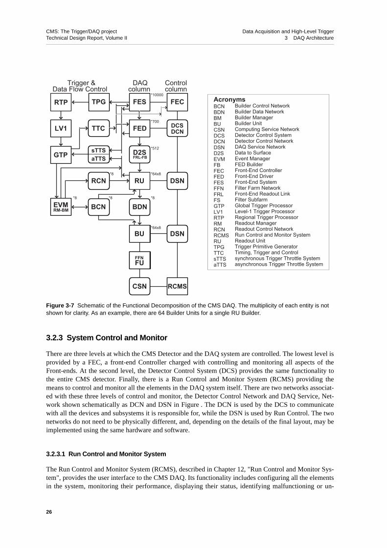
CMS: The Trigger/DAQ project Data Acquisition and High-Level TriggerTechnical Design Report, Volume II 3 DAQ Architecture
3.2.3 System Control and Monitor
There are three levels at which the CMS Detector and the DAQ system are controlled. The lowest level isprovided by a FEC, a front-end Controller charged with controlling and monitoring all aspects of theFront-ends. At the second level, the Detector Control System (DCS) provides the same functionality tothe entire CMS detector. Finally, there is a Run Control and Monitor System (RCMS) providing themeans to control and monitor all the elements in the DAQ system itself. There are two networks associat-ed with these three levels of control and monitor, the Detector Control Network and DAQ Service, Net-work shown schematically as DCN and DSN in Figure . The DCN is used by the DCS to communicatewith all the devices and subsystems it is responsible for, while the DSN is used by Run Control. The twonetworks do not need to be physically different, and, depending on the details of the final layout, may beimplemented using the same hardware and software.
3.2.3.1 Run Control and Monitor System
The Run Control and Monitor System (RCMS), described in Chapter 12, "Run Control and Monitor Sys-tem", provides the user interface to the CMS DAQ. Its functionality includes configuring all the elementsin the system, monitoring their performance, displaying their status, identifying malfunctioning or un-
Figure 3-7 Schematic of the Functional Decomposition of the CMS DAQ. The multiplicity of each entity is not shown for clarity. As an example, there are 64 Builder Units for a single RU Builder.
RTP FECTPG
TTC
sTTSaTTSGTP
LV1 FED
FES
DAQ
ControlTrigger &
DCS
RU
EVMRM-BM
BU
FFNFU
BDN
DCN
DSN
RCMSCSN
DSNRCN
BCN
D2SFRL-FB
column columnData Flow Control
*700
*10000
*512
*64x8
*64x8
*8
*8
*8*8
AcronymsBCNBDNBMBUCSNDCSDCNDSND2SEVMFBFECFEDFESFFNFRLFSGTPLV1RTPRMRCNRCMSRUTPGTTCsTTSaTTS
Builder Control NetworkBuilder Data NetworkBuilder ManagerBuilder UnitComputing Service NetworkDetector Control SystemDetector Control NetworkDAQ Service NetworkData to SurfaceEvent ManagerFED BuilderFront-End ControllerFront-End DriverFront-End SystemFilter Farm NetworkFront-End Readout LinkFilter SubfarmGlobal Trigger ProcessorLevel-1 Trigger ProcessorRegional Trigger ProcessorReadout ManagerReadout Control NetworkRun Control and Monitor SystemReadout UnitTrigger Primitive GeneratorTiming, Trigger and Control synchronous Trigger Throttle Systemasynchronous Trigger Throttle System
26

CMS: The Trigger/DAQ project Data Acquisition and High-Level TriggerTechnical Design Report, Volume II 3 DAQ Architecture
der-performing elements, and providing recovery mechanisms (for instance, resetting and restarting aftera failure). The RCMS also interfaces to the Detector Control System (DCS).
3.2.3.2 Detector Control System
The Detector Control System, described in Chapter 13, "Detector Control System", is responsible for thetraditional control and monitoring of all the detector services and other elements, from high and low volt-age supplies to temperature sensors, as well as with the configuration of the front-end electronics. It is ex-pected that during data-taking the DCS, which is nearly autonomous, will be driven by the RCMS.
3.3 Software Architecture
The architecture of the online-software infrastructure follows a layered middleware approach for distrib-uted systems, designed according to an object-oriented model and implemented using the C++ language.Each computing node runs a copy of an executive program that exposes two sets of interfaces. The firstlies between the middleware and the core plugins, components providing basic access to system servicesand communication hardware. The second lies between the middleware and the applications componentsand provides the access to the functions offered by the core plugins as shown in Figure 3-8. The middle-ware services include data and signal dispatching to applications, data transmission, exception handlingfacilities, access to configuration parameters, application and services location lookup (address resolu-tion) and basic system services. The latter include locking, synchronization, task execution and memorymanagement facilities. Applications communicate with each other through the services provided by theexecutive according to a peer-to-peer message-passing model. Each application can act both as a clientand as a server. Messages are exchanged according to an event-driven processing scheme [3-1]. Messagesare sent asynchronously and trigger the activation of user supplied procedures when they arrive at the re-ceiver side.
In addition to the software services that support distributed computing, the online software includes com-ponents to support local tasks such as hardware access, database access and local data monitoring. TheHardware Access Library (HAL) is used to directly manipulate hardware devices for configuration pur-poses. It provides access to registers and memory areas for various bus systems through named objectsthat can be defined dynamically.
Figure 3-8 Architecture of the online software.
Interface
Application Component
Application Component
Executive DatabaseAccessLibrary
Hardware AccessLibrary
DataMonitoring
Library
CommunicationComponent
SystemServices
Interface Interface Interface Interface
27

CMS: The Trigger/DAQ project Data Acquisition and High-Level TriggerTechnical Design Report, Volume II 3 DAQ Architecture
The Database Access Library (DAL) exhibits an interface to read information from persistent data storesand presents it to the user through a standardized interface, the Document Object Model (DOM) [3-2].DOM renders information as trees that can be traversed by the application code. Each node can contain anamed data element or may be a link to other information that is accessible through one of the providedprotocols. The library provides the required authentication and access regulation procedures for each sup-ported persistent data store.
A library is used to perform basic statistical analysis for monitoring the applications’ and system’s opera-tion on a local processing node. It allows the results to be rendered in a standard description, suitable forstorage with database systems and for visualization using common display facilities supported by Webbrowsers.
The above software packages can be combined to retrieve parameters for a particular device from a data-base to configure, monitor and control the hardware at run-time.
The online-software is based on various industry standards for data-exchange to reduce development andmaintenance efforts as well as to achieve interoperability with external systems. The selected technolo-gies, through their wide adoption, increase the confidence to reach working solutions whether functions,services or whole subsystems are to be replaced. As an example of such a standard, the interface to exter-nal systems, such as run-control and monitoring facilities has adopted the Simple Object Access Protocol(SOAP)[3-3]. This message-passing protocol relies on the HTTP Web protocol [3-4] and encapsulatesdata using the eXtensible Markup Language (XML) [3-5]. More details are provided in Chapter 10, "On-line Software".
3.4 High-Level Trigger
The algorithms used for the event selection, along with the details of the software and the detector simu-lation used to evaluate the performance of these algorithms, are described in Chapter 14, "Detector Simu-lation and Reconstruction" and in Chapter 15, "Physics Object Selection and HLT Performance".
As explained in the introduction, the CMS processor farm executes algorithms that combine the tradition-al “Level-2” and “Level-3” trigger steps. The wish to offer as much physics selection flexibility as possi-ble, given the financial and technical constraints of the DAQ project, was one of the guiding principles,and one that results in the current architecture. The basic thesis of the CMS architecture is the creation ofa system that can provide the following to the High-Level Trigger process:
• data which, except for the calibration constants used by the HLT, is essentially of “offline” quality;
• data originating from any part of the detector, without any restrictions from the physical connec-tion of this detector element to some part of the readout or other electronics;
• full algorithmic flexibility, without any limitations arising from programming languages, instruc-tion sets, or other technical limitations often encountered with special-purpose, in-house designs.
The first requirement is obviously satisfied, since the data given to the HLT processors are the full rawdata contained in the front-end electronics, without any loss of information from further digitizationand/or merging of the information. The second requirement is also clearly satisfied, since each processoris connected, by design, to all the detector elements of CMS, and can therefore access any data it deemsvaluable for the selection of any particular event. The third requirement is satisfied since the DAQ pro-vides standard commercial processors as the platform on which the HLT algorithms are run.
28

CMS: The Trigger/DAQ project Data Acquisition and High-Level TriggerTechnical Design Report, Volume II 3 DAQ Architecture
As discussed already, while the above three features result in a HLT system which is only limited by thetotal computing resources that can be procured, a remaining issue is whether the system can provideenough throughput for the entire set of events accepted by the Level-1 Trigger to be forwarded to a givenprocessor in the HLT farm. For the case of the 100 kHz scenario considered so far, the architecture de-scribed in this chapter, using 2Gb/s links can indeed provide this throughput. The demonstration of thisfact is the subject of Part 2 “Data Flow” of this Technical Design Report.
3.5 Summary
The architecture of the CMS DAQ is motivated by the considerations put forth in Chapter 1, "Overview".In summary, it is conceived for a system that is expected to change with time, accelerator and experimentconditions. It is also conceived to provide the maximum possible flexibility to executing a full physics se-lection online. Finally, the two-stage switching design explicitly addresses the varying timescales of theexperiment’s installation and of technological progress over the next few years. The remaining chaptersof this Technical Design Report are aimed at providing a full blueprint of those elements of the DAQ thatmust be present in the middle of 2004, and a full design and proof of principle for those elements thatonly have to be present shortly before the actual start of data taking, currently planned for 2007.
3.6 References
3-1 B. N. Bershad et al., “Extensibility, Safety and Performance in the SPIN Operating System”, in Proceedings of the Fifteenth ACM Symposium on Operating System Principles, pp. 267-284, 1995.
3-2 A. Le Hors et al.,” Document Object Model (DOM) Level 3 Core Specification, Version 1.0, W3C Working Draft 13, September 2001”, http://www.w3.org/TR/2001/WD-DOM-Level-3-Core-20010913
3-3 D. Box et al.,” Simple Object Access Protocol (SOAP) 1.1, W3C Note 08 May 2000”, http://www.w3.org/TR/SOAP
3-4 R. Fielding et al., “Hypertext Transfer Protocol - HTTP/1.1”, IETF RFC 2616, June 1999. http://www.w3.org/Protocols/rfc2616/rfc2616.html
3-5 J. Boyer, “Canonical XML Version 1.0, W3C Recommendation 15 March 2001”, http://www.w3.org/TR/xml-c14n
29

CMS: The Trigger/DAQ project Data Acquisition and High-Level TriggerTechnical Design Report, Volume II 3 DAQ Architecture
30

CMS: The Trigger/DAQ project Data Acquisition and High-Level TriggerTechnical Design Report, Volume II
Part 2Data Flow
31

CMS: The Trigger/DAQ project Data Acquisition and High-Level TriggerTechnical Design Report, Volume II
32

CMS: The Trigger/DAQ project Data Acquisition and High-Level TriggerTechnical Design Report, Volume II 4 Event Builder
4 Event Builder
One of the main tasks of the Data Acquisition (DAQ) system is to read the data corresponding to eachevent selected by the Level-1 Trigger out of the detector Front-End Drivers, to concatenate it into a singledata structure, the “physics event”, and to then forward this event to a filter farm for the final decision onwhether the event should be discarded or directed to permanent storage. The complex that provides thesefunctions, i.e. the detector readout, the merging of the data from the physically and logically distinct datasources, and the forwarding of complete events to a set of processors is referred to as the “Event Builder”.
This chapter provides a functional description of the Event Builder of the DAQ. The emphasis is on thearchitecture, the overall functionality and the interfaces between the individual components of the EventBuilder. The protocols used, as well as the control of the data flow are the subject of Chapter 5, "EventFlow Control". The design of the networks involved in the Event Builder is the subject of Chapter 6,"Event Builder Networks". Finally, the elements comprising the full readout and filtering chain of theDAQ are described in Chapter 7, "Readout Column" and Chapter 8, "Filter Column".
4.1 Introduction
The three main requirements on the Event Building process in the DAQ are summarised in Table 4-1.These are “system-level” parameters, in the sense that they are essentially independent of any designchoices. Thus, the maximum Level-1 Trigger rate of 100,000 Hz as well as the O(102) Hz are dictated bythe physics program of the experiment as well as the expected offline computing resources that will bemade available. Similarly, the average event size is an “external” parameter that is estimated based on theexpected occupancy of the CMS detector channels.
The Event Builder is implemented as a two-stage process as outlined in Chapter 3, "DAQ Architecture".In the first stage, the data for each event in the Front-End Drivers (FEDs) are merged into Readout Units(RUs). The RUs read the data from 8 FEDs, and perform a first concatenation of the event data fragmentsinto larger data blocks, referred to as “super-fragments”, or “s-fragments”. This stage is implemented by64 “FED Builders”, where a FED Builder comprises 8 FEDs, a 8×8 switch and 8 RUs. Data from differ-ent events are sent, in turn, to different RUs, thus maximizing the bandwidth of the readout. At the end ofthis first stage, the data from a single event are contained in 64 RUs. These RUs are in turn read out byBuilder Units (BUs) which combine the 64 super-fragments into a single event. The collection of 64 Rea-dout Units, the 64×64 switch that connects them to the Builder Units and the actual 64 Builder Units is re-ferred to as a “RU Builder”.
The full DAQ system comprises 64 FED Builders and 8 RU Builders as listed in Table 4-2 and displayedin Figure 4-1. The rest of this chapter describes the functionality of these two Builders.
Table 4-1 Requirements of the CMS Event Builder.
Parameter Value
Maximum Level-1 Trigger rate 100,000 Hz
Maximum rate after High-Level Trigger O(102) Hz
Average event size 1 MB
33

CMS: The Trigger/DAQ project Data Acquisition and High-Level TriggerTechnical Design Report, Volume II 4 Event Builder
Table 4-2 Event Builder parameters.
Parameter Value Derived from Scope
Number of inputs to the Event Builder 512 Assumed link speed: 2Gb/s System
Number of Readout Unit Builders 8 Assumed switch size: 64×64Full Event Builder
Number of FED Builders 64 Number of RU Builders
Inputs (FEDs) per FED Builder 8 − 16 Desired mean size at output
FED BuilderAverage FED data fragment size 0.1 − 3 kB Detector readout
Outputs (RUIs) per FED Builder 1 − 8 Number of RU Builders installed
FED Builder output: s-fragment size 16 kB Balancing of data sizes across RUs
Inputs (RUs) per RU Builder 64 Assumed switch size
RU BuilderAverage s-fragment size 16 kB Balancing of inputs: 1MB/64
Outputs (BUs) per RU Builder 64 Number of inputs
Maximum event rate in RU Builder 12.5 kHzNumber of inputs in RU Builder,
link speed
Figure 4-1 Conceptual Design of the Event Builder. This is a “three-dimensional” view of the system. On thefront-side is one Readout Unit (RU) Builder. On the left and down the side is a schematic of the multiple RUBuilders and the way they are connected to the Front-ends via a small switch (8×8) which routes each event tothe appropriate RU Builder. The interface to the Front-ends, the small switch and the input to the RU Builderconstitute the Front-End Driver (FED) Builder.
1
Detector Front-Ends
Front-End Driver (FED) Front-End Readout Link (FRL)
Readout
Units (RU)
Builder
Units (BU)Event
Manager
Global Trigger
Processor
FED Builder Switches
RU Builders (1 to 8)
Controland
Monitor
Readout Builder Network
FED Builders
FilterSub-farms
RU1,1
1
1 1
2
81,64
1,1
1,64
64
BU
512
Filter Farm Network
FU
34

CMS: The Trigger/DAQ project Data Acquisition and High-Level TriggerTechnical Design Report, Volume II 4 Event Builder
4.2 FED Builder
The main functions of the FED Builder are (see Figure 4-2):
1. transport the fragments from the underground area to the surface,
2. assemble event fragments of variable size from some ~700 FEDs into 64 super-fragments (s-frag-ments) of roughly equal size (16kB each),
3. multiplex these s-fragments on an event by event basis between N (1≤N≤8) Readout Unit Builders.
The implementation of the second and third functions necessitates the connection of a number of FEDs(typically 8) to a number of RUs. The full system has 8 RUs, but in general, only one per RU Builderneed be present in the system. The connection is achieved by switches with typically 16 ports, 8 for inputand 8 for output. Each input port obtains data, corresponding to a single event, from one or two FEDs.Each output port is connected to a Readout Unit which concatenates the 8 fragments into a super-frag-ment. When the system is equipped with more than one RU Builder, successive events are multiplexed,via the switch, to different Readout Units and hence different RU Builders. The full system has 64 FEDBuilders, which connect the FEDs to the RUs, plus an additional FED Builder, which connects the GlobalTrigger Processor to the Event Manager of each RU Builder.
Each FED Builder consists of an interface to the FEDs, a Fed Builder Input buffer (FBI), a switch and anoutput buffer. The interface to the FEDs is called the “Front-end Readout Link” (FRL) and the outputbuffer is called the “Readout Unit Input” (RUI) because it also serves as input to the Readout Unit.
To maintain the data rate of the CMS DAQ system, each FED Builder input must sustain the data from asingle FED at a rate of up to 100 kHz, i.e. 2 kB⋅100 kHz = 200 MB/s. Clearly, the switch output portsmust be capable of sustaining this data rate as well, and therefore the basic FED Builder switch consistsof 16 ports each one providing a sustained 200 MB/s.
Figure 4-2 FED Builder elements from FED to RUI plus the special FED Builder connecting the Global TriggerProcessor to the Event manager.
’Side’ view ’Front’ view
1
ReadoutUnits
BuilderUnits
EventManager
Global TriggerProcessor FED
DAQ linksFED Builders
Sub-farms
1
FU
64
BU1 64
512
FED>P
1 8
Filter
Detector Front-Ends
Controland
MonitorReadout Builder Network
Filter Farm Network
RURUI
RUI
BCN
BDN
DSN
RCNLV
1A
aTTS
TTCsTTSTPD
FED
FRLFRL
BUFU
FFN
BDN
EVM
RU
8x8 FB switches
35

CMS: The Trigger/DAQ project Data Acquisition and High-Level TriggerTechnical Design Report, Volume II 4 Event Builder
4.2.1 Front-end Readout Link (FRL)
With 64 switches and 8 input ports per switch, there are only 512 input ports available to connect morethan 600 FEDs. The FRL, whose primary function is to provide the link between the FEDs and the FEDBuilder Input buffer (FBI) can optionally merge data from two FEDs so that the maximum number ofFEDs that can be read out is 1024
The FRL also checks the event fragment size and discards event fragments whose size exceeds a prede-fined maximum. This is necessary in order to protect the FED Builder from problematic events.
The FRL constitutes the interface between the FEDs and the FED Builder and is not considered to be partof the FED Builder.
4.2.2 FED Builder Input Buffer (FBI)
The FBI sends the data received from the FRL to the FED Builder switch and must therefore select thecorrect output port for each event. The algorithm used to determine the destination for each event mayvary from a simple round-robin across all outputs, implemented as modulo 8 of the trigger number, tomore general cases designed to make efficient use of the DAQ when the RU Builders are not identical inperformance. If the RU Builders are installed in stages, it is possible and likely that the newer ones canoperate at higher performance than those installed in the beginning. The algorithm for selecting a destina-tion can be used to send more events to the faster RU Builders. The algorithm can also be used to redirectdata traffic away from a RU Builder that has developed a fault.
4.2.3 FED Builder Switch
The FED Builder switch provides the inter-connectivity between the FBIs and the RUIs in the CMS Rea-dout. In its simplest configuration, it is a 16-port switch capable of sustaining 200 MB/s per port. This8×8 switch1 has eight ports connected to FBIs and eight ports connected to RUIs. In reality, the actualnumber of FBIs connected to a single FED Builder will not be fixed to eight, but will be determined bythe average size of the data fragments in the corresponding FEDs. In particular, the FED event fragmentsize, as discussed in Section 7.2, "Detector Readout Requirements", varies significantly across FEDs,with some FEDs providing an average fragment size as low as 100 B. Each FED Builder switch will con-nect to FEDs with both small and large event fragment sizes selected such that the sum of the fragmentsizes in each switch is approximately equal across the RUs.
In addition to differences in the average amount of data from different FEDs, the actual amount of datafrom a single FED fluctuates from event to event. As explained in Section 6.2.3, "Traffic-shaping", thisvariability of the data size leads to a lower utilization efficiency of the switch bandwidth. For this reason,one must either apply some traffic-shaping policy or provide switches with port capacity which is suffi-ciently larger than the desired throughput. To avoid complicated traffic patterns at this early stage of theDAQ, the FED switches are required to have ports running at twice the desired average of 200 MB/s, i.e.the FED Builder switch should have 400 MB/s per port.
A final requirement on the FED Builder switch is that the overall network (FRL-Switch-RU) it belongs toshould provide back pressure so that data are not lost in case of congestion in the system downstream.
1. In general, it is an “n×m” switch where 1≤n≤16 and 1≤m≤16. The final values of n, m are an implementation issue.At present, the most likely option, used throughout this TDR in order to simplify the description, is the case n=m=8.
36

CMS: The Trigger/DAQ project Data Acquisition and High-Level TriggerTechnical Design Report, Volume II 4 Event Builder
4.2.4 The Readout Unit Input (RUI)
The output of the FED Builder serves as input to the Readout Unit and is thus given the name “ReadoutUnit Input” (RUI). As mentioned above, the basic function of the RUI is to build super-fragments fromthe collection of event fragments from the FEDs and to transmit these s-fragments to the RU. This is de-scribed in more detail in “4.3.7 RU Builder Data Flow”. The RUI consists of a processor with sufficientmemory to build and store super-fragments. It has high bandwidth data connections to both the FEDBuilder switch and the Readout Unit.
4.2.5 Data Flow in the FED Builder
The protocol used by the FED to send event fragments to the FRL is made as simple as possible: upon re-ceipt of a Level-1 Trigger accept, the FED encapsulates the event data corresponding to the bunch cross-ing in question in a common CMS data format1 and stores it in its FIFO output buffer. The encapsulationheader includes the event number which is used by the FBI to route the fragment through the FED switch.Event data flow from the output buffer of the FED through the FRL to the FBI, whenever data are presentin the FIFO and the FBI is ready to receive. The protocol used includes control words that are used by theFRL to recognize the start and end of each event fragment. The data flow includes backpressure so datawill stop flowing if the FRL and FBI buffers fill up. Note that this will in turn cause the FIFO in the FEDto fill up. To prevent new triggers while the DAQ has no room for more data, the FED will issue a fasttrigger-throttling signal when the FIFO of the FED is filled beyond a pre-defined high level mark.
In the simplest and most common case the FRL receives input from only one FED and passes it throughto the FBI. The FBI then extracts the event number from the FED data and determines, based on thisnumber2, the destination RUI (i.e. the switch output port number). It then transmits the fragment to thatoutput port. The algorithm used for calculating the output port number is identical in all the 512 FBIs.Output ports corresponding to the same event number in all 64 FED Builder switches belong to one RUBuilder. In the more complicated case where the FRL receives data from more than one FED, these frag-ments are merged in the FRL before they are passed through to the FBI.
4.2.5.1 “Super-fragment” Building
For a given trigger the data fragments from the 8 input ports of a FED Builder switch arrive at the outputport (RUI) in an arbitrary order, depending on the switch load, the timing of the start of sending and thesizes of the FRL fragments. The RUI has a processor with memory and the fragments are stored in thismemory in the order in which they arrive. Once all fragments have arrived they are assembled into a “su-per-fragment” (s-fragment). A header containing the event number and the s-fragment size is then addedto each s-fragment. The s-fragments are transferred to the memory of the RU in order of increasing eventnumber as soon as they have been assembled. This is done in order to free space for new event fragmentsin the RUI which has limited memory. In this scheme, it is the RUI that is responsible for the transfer ofthe s-fragments to the RU in an ascending event number order.
The FED Builder switch supports backpressure. This in turn causes backpressure from the FBI to the FRLto the FEDs and data stops flowing. This can happen even if only one output port, i.e. any one of the 8 Re-
1. See Section 7.3.3, "FED Data Format".
2. As previously mentioned, the algorithm used to select the destination RUI can be anything from a simpleround-robin to a more sophisticated algorithm that allows for un-equal data distributions among the switch outputs.This latter case can be implemented using, e.g. “destination tables” prefabricated by the Run Control system.
37

CMS: The Trigger/DAQ project Data Acquisition and High-Level TriggerTechnical Design Report, Volume II 4 Event Builder
adout Units, blocks the data flow. If one RU Builder develops problems that cause it to block the dataflow frequently or permanently, then the system is reconfigured to exclude this RU Builder from the listof outputs of all FED Builders and data taking is then resumed with the reduced capacity provided by theremaining RU Builders
The fragment size from a given FED varies from event to event. These statistical fluctuations can be ab-sorbed by the FED Builder within certain limits imposed by the link speed and the amount of memoryavailable for s-fragment building. A truncated version of the fragment, flagged as an error is transmittedwhen a fragment must be discarded because it is too big.
4.2.6 FED Builder for the Global Trigger Processor
A few entities from the global trigger, such as event number, bunch crossing number and trigger pattern,must be read by the Event Manager at each Level-1 Trigger, very much in the same way that event frag-ments are read from the FEDs at each trigger. This data must be routed to the Event Manager in the sameRU Builder as the FED data for the event and must therefore also go through a FED Builder.
The FED Builder for the Global Trigger is special in the sense that it does no merging of data. Only oneinput port, connected to the Global Trigger, is used. There are up to 8 output ports, one for each RUBuilder in the DAQ system. Each output port is connected to the corresponding Event Manager.
The Global Trigger also provides trigger data in three additional data streams (GT data, CalTrig Data,MuTrig Data). These data are considered to part of the event data and are thus read like data from any oth-er FED.
4.3 RU Builder
The second stage of the Event Building process is carried out by up to eight RU Builders (see Figure 4-3).The function of the RU Builder is to assemble the event super-fragments from the 64 FED Builders intofull events ready for processing in the filter farm. The main functional elements of the RU Builder are:
• 64 Readout Units (RUs) with large buffers that serve to de-couple the flow of data out of the FEDsfrom the flow of data in to the RU Builder.
• 64 Builder Units (BUs) where full events are assembled and then sent off to the filter farm
• 1 Event Manager, whose primary function is to adapt the traffic in the RU Builder to the through-put capacity of the BUs and their associated filter farms.
• 3 logical networks connecting the storage and processing elements
a. Builder Control Network (BCN). Connects all units in the system and whose main functionis to enable the flow of control information.
b. Builder Data Network (BDN). The high-throughput network used for the transfer of theevent data. It connects all the RUs to all the BUs.
c. Readout Control Network (RCN).Connects the Event Manager to all the RUs. It serves todistribute common Readout information to all the RUs
Each of these elements are briefly described in the following sections. The detailed description of the dataflow in Section 4.3.7, "RU Builder Data Flow" should help explain the interconnection between these el-ements.
38

CMS: The Trigger/DAQ project Data Acquisition and High-Level TriggerTechnical Design Report, Volume II 4 Event Builder
4.3.1 Requirements
Table 4-2 shows how the global event building parameters, along with a basic assumption for the size ofthe switch with 2Gb/s links that will be available, translate into requirements for the RU Builder. Theserequirements need not be met until a few years after the start of LHC operations since it is expected that atthe beginning of data taking in 2007, the accelerator will operate at a reduced luminosity with potentiallysome detector elements to be installed at a later time. In 2007 the average data rate is anticipated to be ap-proximately a factor 3-5 smaller than the design requirement of 100 GB/s (100 kHz⋅1 MB).
Since the final system consists of up to eight RU Builders, each RU Builder must sustain an event rate ofup to 12.5 kHz. This corresponds to a data throughput of 12.5 kHz ⋅ 16 kB = 200 MB/s for each RU. Atthe start of data taking in 2007 when only a few RU Builders will be needed, the maximum throughputper RU will still be 200 MB/s.
4.3.2 Readout Unit (RU)
The RU performs three functions: it reads super-fragments (s-fragments) from the RUI, buffers them inits memory until a request for this data is made and finally transmits the data to the Builder Units (BU)upon request. In Figure 4-4 the RUs are shown in the context of the RU Builder.
The primary function of the RU is to provide sufficient buffer space to store s-fragments until the fullevent data corresponding to each event are assembled in the corresponding Builder Unit. A secondaryfunction is to allow for an efficient use of the Builder Data Network via the implementation of trafficshaping and optimal data organization in memory. A final function of the RU is to check the correctnessof the data concentration performed by the FED Builder.
Up to the input buffer of the RUs all buffering in the readout is carried out in hardware or software FIFOswhich contain, in the header information of each fragment, the bunch crossing number and the eventnumber. After this point, random access is required because the BUs operate in parallel. The RU must
Figure 4-3 Event builder with the RU Builder highlighted.
’Side’ view ’Front’ view
1
Global TriggerProcessor
FED
DAQ linksFED Builders
Sub-farmsFU
64
512
FED>P
1 8
Filter
8x8 FB switches
ReadoutUnits
BuilderUnits
EventManager
1 64
BU1
RU
BU
FUFF
NB
DN
EVM
RU
Detector Front-Ends
Controland
MonitorReadout Builder Network
Filter Farm Network
BCN
BDN
DSN
RCN
LV1A
aTTS
TTCsTTSTPD
39

CMS: The Trigger/DAQ project Data Acquisition and High-Level TriggerTechnical Design Report, Volume II 4 Event Builder
therefore store event s-fragments in memory in a way that permits efficient random access by the BUs.The RU must also sustain a s-fragment rate of 12.5 kHz, reading s-fragments of 16 kB average size. Thistranslates into a data input rate of 200 MB/s (12.5 kHz ⋅ 16 kB).
After storage in the RU’s memory, the event s-fragment is assigned a temporary Event Identifier(Event_ID), which is the label used for all further references to this event throughout the Readout Builder.
4.3.2.1 Event_ID
This is a logical entity introduced to facilitate efficient random access to event s-fragments in the RU’smemory. It is a unique label assigned to each event after the s-fragments are stored in the RU. The labelremains valid as long as the event is being processed by the event builder (and filter farm). The number ofEvent_IDs is limited and reflects the number of events that can be processed concurrently in the eventbuilder. When an Event_ID becomes free it can be reused for a new event. The use of the Event_ID is de-scribed in Section 4.3.7, "RU Builder Data Flow".
4.3.3 Builder Unit (BU)
The primary event building function of the BU is to build full events from the event s-fragments residingin the 64 RUs. A secondary function is to buffer these events until they are processed by the filter farm.The functionality of the BU with respect to the filter farm is described in Chapter 8.3, "Builder Unit(BU)". This chapter does not deal with the filter farm. It just assumes that the events reside in the BU untilthey have been released by the filter farm. In Figure 4-5 the BUs are shown in the context of the RUBuilder.
Each BU requests event fragments from all the RUs to form one full event. All BUs are active at the sametime, each reading event fragments from the RUs in order to keep the switching fabric operating at fullcapacity. Each BU is actually building multiple events concurrently in order to be able to overlap data in-put with processing. This is described in more detail in Section 4.3.7, "RU Builder Data Flow".
Figure 4-4 RU Builder with RU highlighted.
BCN
BDN
DSN
RCN
LV1A
aTTS
TTCsTTSTPD
’Side’ view ’Front’ view
1
Global TriggerProcessor
FED
DAQ linksFED Builders
Sub-farmsFU
64
512
FED>P
1 8
Filter
8x8 FB switches
ReadoutUnits
BuilderUnits
EventManager
BU1
FUFF
NBD
NEV
MBU
RURUI
64RU
1
Detector Front-Ends
Controland
MonitorReadout Builder Network
Filter Farm Network
40

CMS: The Trigger/DAQ project Data Acquisition and High-Level TriggerTechnical Design Report, Volume II 4 Event Builder
The BU must be able to receive s-fragments of average size of 16 kB from 64 RUs at a rate of12,500/64 = 200 Hz. With an average event size of 1 MB this translates into an input rate of 200 MB/s.
4.3.4 Event Manager (EVM)
The Event Manager (EVM) is the entity, present in each RU Builder, which determines the flow of data inthe RU Builder. Its main function is the assignment of Event_IDs to the events entering the RU Builder,as well as the management of these Event_IDs for the duration of the event’s presence in the RU Builder.The EVM is thus the single entity in the RU Builder that contains the status of all the events in the RUBuilder at any point in time. It is thus the natural place to accumulate system-level statistics related to therate of input events, rate of absorption of events by the filter farm, etc. The EVM communicates with allRUs and BUs in the RU Builder. As mentioned previously (Section 4.2.6, "FED Builder for the GlobalTrigger Processor"), the EVM communicates with the Global Trigger via a standard RUI which serves asthe interface to the FED Builder of the Global Trigger Processor. In Figure 4-6 the EVM is shown in thecontext of the RU Builder.
The EVM consists of two tightly coupled functional units: the Readout Manager (RM) and the BuilderManager (BM). The Readout manager distributes event numbers with an associated Event_ID to all theRUs, while the Builder manager communicates with all the BU’s, distributing valid Event_ID’s on re-quest from the BUs. The two parts share access to a common pool of Event_ID’s.
4.3.5 Builder Network
The Builder Network covers the two logical networks namely the Builder Data Network (BDN) and theBuilder Control Network (BCN). It is a 64×64 port switching fabric connecting the 64 RUs to the 64 BUsin a RU Builder. The switch must be capable of 200 MB/s throughput on each port. Event building is per-formed over this network by sending s-fragments, corresponding to a single event, from all 64 RUs to asingle BU. High performance is achieved by having all 64 BUs collect event fragments from multipleevents concurrently. Inefficiencies may occur in the switching fabric because of congestion at either theoutput ports or in the switch fabric. However with well balanced input and careful traffic shaping it is pos-
Figure 4-5 RU Builder with BU highlighted.
BCN
BDN
DSN
RCN
LV1A
aTTS
TTCsTTSTPD
’Side’ view ’Front’ view
1
Global TriggerProcessor
FED
DAQ linksFED Builders
Sub-farmsFU
64
512
FED>P
1 8
Filter
8x8 FB switches
ReadoutUnits
BuilderUnits
EventManager
1 64
BU1
RU
BU
FUFF
NBD
NEV
MR
U
Detector Front-Ends
Controland
MonitorReadout Builder Network
Filter Farm Network
41

CMS: The Trigger/DAQ project Data Acquisition and High-Level TriggerTechnical Design Report, Volume II 4 Event Builder
sible to operate the switch at almost 100% efficiency. This is discussed extensively in Chapter 6, "EventBuilder Networks". Assuming that such a high utilization of the switch is possible, the switch utilizedneed therefore have a capacity of 200 MB/s per port.
4.3.6 Readout Control Network (RCN)
This is the logical network that connects the EVM to all the RUs in a RU Builder. It may be implementedas an independent network or it may use the same switching fabric as the Builder Network. For each trig-ger the EVM must distribute the Event_ID-event number association to all the RUs. This is not a highvolume of traffic (16 B ⋅ 12.500 Hz = 200 kB/s).
4.3.7 RU Builder Data Flow
The association of Event_IDs with event numbers is performed by the EVM, which manages a pool ofEvent_IDs and associates free ones with event- and bunch crossing numbers, read from the Global Trig-ger at each Level-1 Trigger.
The EVM obtains the trigger information including the event and bunch crossing number from the GlobalTrigger at each Level-1 Trigger directed to the RU Builder in question. The EVM then assigns anEvent_ID to each of these triggers and sends this assignment to all RUs in the RU Builder via the “Read-out Control Network” (RCN). Several assignments may be packed into one physical message over theRCN in order to reduce transmission overheads.
The super-fragments are initially stored in order of arrival in the RU memory, which is also in increasingevent number order, because that is how they are delivered by the RUI. The RU will change this to storethe event fragments indexed by Event_ID as soon as the Event_ID assignments arrive.
The RU buffer memory imposes an upper limit on the maximum latency of the RCN. However, with anaverage data rate into the RU of 200 MB/s and a RU buffer size of O(100) MB, the latency requirement isnot critical. See Chapter 6.6, "Readout Control Network" for a quantitative description.
Figure 4-6 RU Builder with EVM highlighted.
BCN
BDN
DSN
RCN
LV1A
aTTS
TTCsTTSTPD
’Side’ view ’Front’ view
1
Global TriggerProcessor
FED
DAQ linksFED Builders
Sub-farmsFU
64
512
FED>P
1 8
Filter
8x8 FB switches
ReadoutUnits
BuilderUnits
EventManager
1 64
BU1
RU
BUFU
FFN
BD
NEV
MR
U
RUI
Detector Front-Ends
Controland
MonitorReadout Builder Network
Filter Farm Network
42
CMS: The Trigger/DAQ project Data Acquisition and High-Level TriggerTechnical Design Report, Volume II 4 Event Builder
The BU must have access to a list of Event_IDs corresponding to events that are buffered in the RUsawaiting event building. The BU obtains this information from the Event Manager over the “Builder Con-trol Network” (BCN). This ensures that each BU gets allocated a different set of Event_IDs, so that thesame event is not built by two different BUs. The BU can then use an Event_ID to request all the RUs tosend the super-fragment corresponding to this Event_ID. For efficiency reasons the request is not madefor a single Event_ID, but for several Event_IDs that were already allocated to the BU.
All the RUs then start to send s-fragments corresponding to the requested Event_IDs to the BU requestingthem. This can potentially lead to inefficiencies in the BDN network because of congestion at the BU portsince this port is now the target of numerous RUs. Traffic shaping can minimise this congestion andachieve a very high utilization efficiency of the BDN, provided the input traffic is well balanced. The de-tails of this are discussed in Section 6.2, "Event Building with Switching Networks".
The procedure outlined above is followed by all the BUs concurrently, so the BDN has data flowing fromall input ports (RUs) to all output ports (BUs) concurrently.
When a BU (and the associated filter farm) has finished processing an event it requests the EVM to purgethe corresponding Event_ID from all EVB components. The EVM is then free to reuse that Event_ID fora new event accepted by the Level-1 Trigger. The EVM throttles the Level-1 Trigger if the number of freeEvent_IDs falls below some number deemed necessary for the operation of the system in the followingsecond or so.
The EVM communicates with each BU over the “Builder Control Network” (BCN) in a peer-to-peerfashion. Each BU requests a group of Event_IDs and gets a list of Event_IDs in return. The communica-tion between the EVM and the RUs over the RCN may be one-to-N, or peer-to-peer, depending on switchtechnology.
The BU has enough memory to concurrently build several events from all RUs plus sufficient memory tobuffer events that are currently in use in the filter farm. Whenever buffer space is available in the BU formore events, the BU requests new Event_IDs from the Event Manager. As already mentioned, this is notdone on an event by event basis, but when a given fraction of the available buffer space has been released.This grouping of requests reduces the load on the Event Manager, which must communicate with all BUsindividually.
4.4 Partitioning
In normal physics data acquisition mode the event builder works as described so far in this chapter. How-ever other modes must also be possible in order to cover the following cases
• Some detectors need to take data independently of the others for the purpose of
• Calibration
• Detector or trigger commissioning
• DAQ debugging
• All detectors participate in normal physics data taking except for one which may perform any ofthe tasks listed above.
The division of the DAQ into smaller subsets capable of operating (more or less) independently of eachother is called partitioning. Partitions used for calibration or commissioning have less stringent event raterequirements than physics data taking so efficient event building is not a requirement.
43

CMS: The Trigger/DAQ project Data Acquisition and High-Level TriggerTechnical Design Report, Volume II 4 Event Builder
The CMS trigger system must also be partitioned to provide independent triggers to each of the DAQ par-titions. The partitioning of the CMS trigger is described in reference [4-1]. The partitioning of the triggerimposes constraints on the partitioning of the DAQ system as well and for this reason it is described brief-ly in the following section.
4.4.1 Trigger Partitioning
The CMS trigger system is organised in 32 partitions, with each partition corresponding to a major com-ponent of a subdetector to which triggers are distributed and from which Trigger-Throttling System (TTS)signals are collected. These partitions are referred to as Trigger Timing and Control (TTC) partitions inthis document. The TTC partitions can be grouped in up to 8 TTC partition groups, which can operate in-dependently.
The configuration and operation of these TTC partition groups is carried out under the control of the Glo-bal Trigger Processor. Each TTC partition group operates with its own trigger conditions, receiving trig-gers that correspond to these conditions only. The triggers are distributed to just one TTC partition groupat a time.
TTC partitions from different subdetectors may be combined in one TTC partition group. All TTC parti-tions are integrated into a single TTC partition group when the DAQ system is running in normal physicsconditions.
The Global Trigger Processor receives triggers from all the TTC partition groups and sends them to theEvent Managers in the RU Builders. The DAQ must be configured to have one DAQ partition corre-sponding to each TTC partition group and the DAQ design must allow independent operation of eachDAQ partition.
4.4.2 DAQ Partitioning
The DAQ system is designed to have one DAQ partition for each TTC partition group of the Global Trig-ger. Each DAQ partition can operate independently of the other DAQ partitions in terms of data flow andrun control. That is to say each DAQ partition can start and stop runs without forcing the other DAQ par-titions to start and stop at the same time and a data flow problem in one DAQ partition will not preventdata from flowing in the other DAQ partitions.
The required independence of the DAQ partitions imposes some limitations on their granularity.
• A RU can not belong to more than one partition
• It is preferable that each partition has its own EVM
The DAQ partitioning can be implemented either at the FED Builder level, assigning RU Builders to bepartitions, or at the RU Builder level dividing each RU Builder into partitions. Both methods are de-scribed in the following sections.
4.4.2.1 FED Builder Partitioning
The distribution of events to RU Builders is performed by programmable logic in the FED Builder as de-scribe in Section 4.2, "FED Builder". Events are normally distributed to different RU Builders as deter-mined by the event number modulo the number of RU Builders active in the system. However, a group of
44
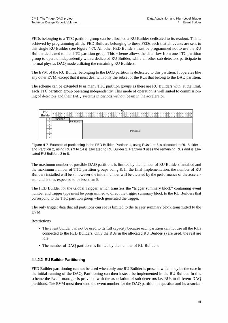
CMS: The Trigger/DAQ project Data Acquisition and High-Level TriggerTechnical Design Report, Volume II 4 Event Builder
FEDs belonging to a TTC partition group can be allocated a RU Builder dedicated to its readout. This isachieved by programming all the FED Builders belonging to these FEDs such that all events are sent tothis single RU Builder (see Figure 4-7). All other FED Builders must be programmed not to use the RUBuilder dedicated to that TTC partition group. This scheme allows the data flow from one TTC partitiongroup to operate independently with a dedicated RU Builder, while all other sub detectors participate innormal physics DAQ mode utilizing the remaining RU Builders.
The EVM of the RU Builder belonging to the DAQ partition is dedicated to this partition. It operates likeany other EVM, except that it must deal with only the subset of the RUs that belong to the DAQ partition.
The scheme can be extended to as many TTC partition groups as there are RU Builders with, at the limit,each TTC partition group operating independently. This mode of operation is well suited to commission-ing of detectors and their DAQ systems in periods without beam in the accelerator.
The maximum number of possible DAQ partitions is limited by the number of RU Builders installed andthe maximum number of TTC partition groups being 8. In the final implementation, the number of RUBuilders installed will be 8, however the initial number will be dictated by the performance of the acceler-ator and is thus expected to be less than 8.
The FED Builder for the Global Trigger, which transfers the “trigger summary block” containing eventnumber and trigger type must be programmed to direct the trigger summary block to the RU Builders thatcorrespond to the TTC partition group which generated the trigger.
The only trigger data that all partitions can see is limited to the trigger summary block transmitted to theEVM.
Restrictions
• The event builder can not be used to its full capacity because each partition can not use all the RUsconnected to the FED Builders. Only the RUs in the allocated RU Builder(s) are used, the rest areidle.
• The number of DAQ partitions is limited by the number of RU Builders.
4.4.2.2 RU Builder Partitioning
FED Builder partitioning can not be used when only one RU Builder is present, which may be the case inthe initial running of the DAQ. Partitioning can then instead be implemented in the RU Builder. In thisscheme the Event manager is provided with the association of sub-detectors i.e. RUs to different DAQpartitions. The EVM must then send the event number for the DAQ partition in question and its associat-
Figure 4-7 Example of partitioning in the FED Builder. Partition 1, using RUs 1 to 8 is allocated to RU Builder 1and Partition 2, using RUs 9 to 14 is allocated to RU Builder 2. Partition 3 uses the remaining RUs and is allo-cated RU Builders 3 to 8.
0 0 0 0 0 0 0 0 0 1 1 1 1 1 1 1 1 1 1 2 2 2 2 2 2 2 2 2 2 3 3 3 3 3 3 3 3 3 3 4 4 4 4 4 4 4 4 4 4 5 5 5 5 5 5 5 5 5 5 6 6 6 6 61 2 3 4 5 6 7 8 9 0 1 2 3 4 5 6 7 8 9 0 1 2 3 4 5 6 7 8 9 0 1 2 3 4 5 6 7 8 9 0 1 2 3 4 5 6 7 8 9 0 1 2 3 4 5 6 7 8 9 0 1 2 3 4
12345678
RURU Builder
Partition 2
Partition 3
Partition 1
45
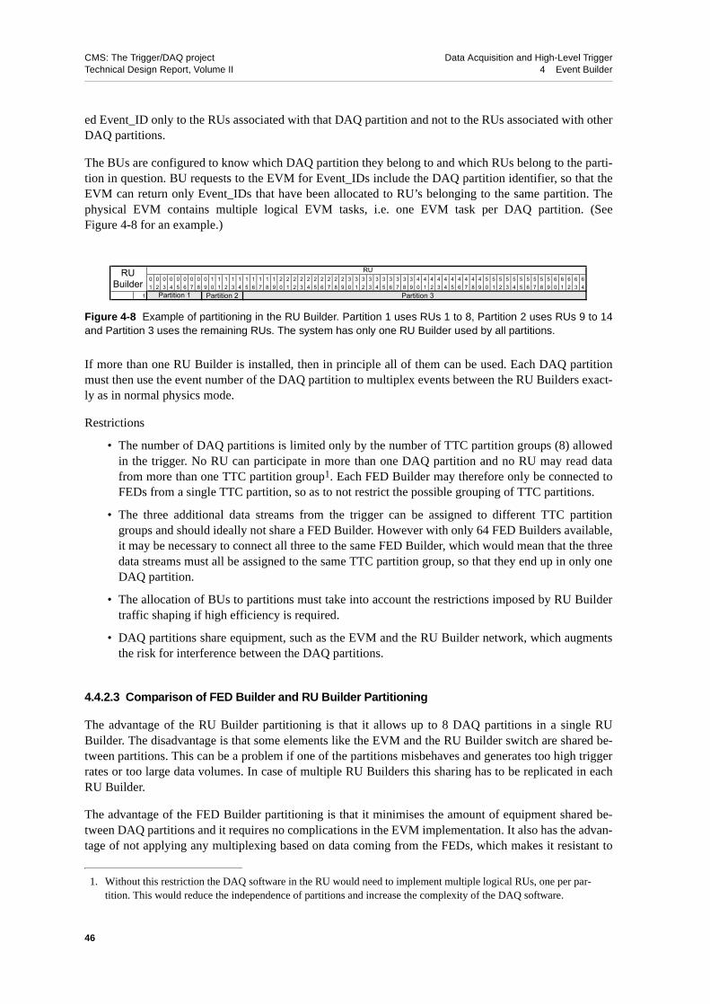
CMS: The Trigger/DAQ project Data Acquisition and High-Level TriggerTechnical Design Report, Volume II 4 Event Builder
ed Event_ID only to the RUs associated with that DAQ partition and not to the RUs associated with otherDAQ partitions.
The BUs are configured to know which DAQ partition they belong to and which RUs belong to the parti-tion in question. BU requests to the EVM for Event_IDs include the DAQ partition identifier, so that theEVM can return only Event_IDs that have been allocated to RU’s belonging to the same partition. Thephysical EVM contains multiple logical EVM tasks, i.e. one EVM task per DAQ partition. (SeeFigure 4-8 for an example.)
If more than one RU Builder is installed, then in principle all of them can be used. Each DAQ partitionmust then use the event number of the DAQ partition to multiplex events between the RU Builders exact-ly as in normal physics mode.
Restrictions
• The number of DAQ partitions is limited only by the number of TTC partition groups (8) allowedin the trigger. No RU can participate in more than one DAQ partition and no RU may read datafrom more than one TTC partition group1. Each FED Builder may therefore only be connected toFEDs from a single TTC partition, so as to not restrict the possible grouping of TTC partitions.
• The three additional data streams from the trigger can be assigned to different TTC partitiongroups and should ideally not share a FED Builder. However with only 64 FED Builders available,it may be necessary to connect all three to the same FED Builder, which would mean that the threedata streams must all be assigned to the same TTC partition group, so that they end up in only oneDAQ partition.
• The allocation of BUs to partitions must take into account the restrictions imposed by RU Buildertraffic shaping if high efficiency is required.
• DAQ partitions share equipment, such as the EVM and the RU Builder network, which augmentsthe risk for interference between the DAQ partitions.
4.4.2.3 Comparison of FED Builder and RU Builder Partitioning
The advantage of the RU Builder partitioning is that it allows up to 8 DAQ partitions in a single RUBuilder. The disadvantage is that some elements like the EVM and the RU Builder switch are shared be-tween partitions. This can be a problem if one of the partitions misbehaves and generates too high triggerrates or too large data volumes. In case of multiple RU Builders this sharing has to be replicated in eachRU Builder.
The advantage of the FED Builder partitioning is that it minimises the amount of equipment shared be-tween DAQ partitions and it requires no complications in the EVM implementation. It also has the advan-tage of not applying any multiplexing based on data coming from the FEDs, which makes it resistant to
Figure 4-8 Example of partitioning in the RU Builder. Partition 1 uses RUs 1 to 8, Partition 2 uses RUs 9 to 14and Partition 3 uses the remaining RUs. The system has only one RU Builder used by all partitions.
1. Without this restriction the DAQ software in the RU would need to implement multiple logical RUs, one per par-tition. This would reduce the independence of partitions and increase the complexity of the DAQ software.
0 0 0 0 0 0 0 0 0 1 1 1 1 1 1 1 1 1 1 2 2 2 2 2 2 2 2 2 2 3 3 3 3 3 3 3 3 3 3 4 4 4 4 4 4 4 4 4 4 5 5 5 5 5 5 5 5 5 5 6 6 6 6 61 2 3 4 5 6 7 8 9 0 1 2 3 4 5 6 7 8 9 0 1 2 3 4 5 6 7 8 9 0 1 2 3 4 5 6 7 8 9 0 1 2 3 4 5 6 7 8 9 0 1 2 3 4 5 6 7 8 9 0 1 2 3 4
1
RU
Partition 1 Partition 2 Partition 3
RUBuilder
46

CMS: The Trigger/DAQ project Data Acquisition and High-Level TriggerTechnical Design Report, Volume II 4 Event Builder
incorrect event counting in the FEDs. The disadvantages are that only few RU Builders may be installedat the start of LHC operation, where the need for partitioning may be highest, and resources maybe wast-ed because each partition can only use the RUs in its allocated RU Builder(s).
The FED Builder partitioning is the favoured scheme because it minimises the amount of shared equip-ment and the design is simpler. Not only will this minimise the risk of interference between partitions, itshould also make it easier operationally to allow one partition to start and stop runs while others continuerunning. The FED Builder partitioning also allows a finer granularity of the DAQ partitions because itdoes not impose the restriction of only one TTC partition per FED Builder.
4.4.2.4 Combining the two Partitioning Schemes
The RU Builder partitioning is necessary, when the DAQ has only one RU Builder, but it does not lend it-self well to a multi-RU Builder configuration. The FED Builder partitioning only works with multiple RUBuilders, but may be too limited if the number of RU Builders is small.
It is possible to combine the two schemes in several ways (see Figure 4-9). If for instance only four RUBuilders were implemented and it were desired to run with 5 DAQ partitions, then the FED Builder parti-tioning could be used to assign 1 DAQ partition to each of the four RU Builders plus one additional DAQpartition to one of the four RU Builders. The RU Builder with two DAQ partitions would then need RUpartitioning to cope with the two partitions.
4.5 Summary
This chapter has described the two-stage event builder at the functional level. It has defined the require-ments on the FED and RU switches and demonstrated that the performance scales with the number of RUBuilders. Not all RU Builders will be needed at start-up, when the detector and accelerator will operatewell below the nominal values assumed for a full-scale event builder.
It has been demonstrated that the event builder can be partitioned to match the partitioning scheme of thetrigger allowing for independent data flows in each partition.
The chapter on event builder networks will demonstrate that this design can be implemented with currenttechnology and that it can also take advantage of future improvements in switching technology.
4.6 References
4-1 CMS Trigger/DAQ group, ed. J. Varela, “CMS L1 Trigger Control System”, CMS Note 2002/033.
Figure 4-9 Combining the two partitioning schemes. Partitions 1 and 2 in RU Builder 1 require the RU partition-ing scheme to share RU Builder 1, while the other DAQ partitions get assigned their own RU Builders in the FEDBuilder partitioning scheme.
0 0 0 0 0 0 0 0 0 1 1 1 1 1 1 1 1 1 1 2 2 2 2 2 2 2 2 2 2 3 3 3 3 3 3 3 3 3 3 4 4 4 4 4 4 4 4 4 4 5 5 5 5 5 5 5 5 5 5 6 6 6 6 61 2 3 4 5 6 7 8 9 0 1 2 3 4 5 6 7 8 9 0 1 2 3 4 5 6 7 8 9 0 1 2 3 4 5 6 7 8 9 0 1 2 3 4 5 6 7 8 9 0 1 2 3 4 5 6 7 8 9 0 1 2 3 4
1234
RURUBuilder
Partition 2 Partition 1 Partition 3
Partition 4Partition 5
47

CMS: The Trigger/DAQ project Data Acquisition and High-Level TriggerTechnical Design Report, Volume II 4 Event Builder
48

CMS: The Trigger/DAQ project Data Acquisition and High-Level TriggerTechnical Design Report, Volume II 5 Event Flow Control
5 Event Flow Control
Event Flow Control serves to regulate the dataflow from the trigger driven readout of the front-end sys-tems to the demand driven delivery of full events to the Filter farms. It also serves to protect against over-flow of intermediate buffers which might cause loss of synchronisation.
This chapter first describes the event flow control issues from Front-End Systems to the Builder Units andthen concentrates on the implementation of the Event Manager, which performs a central role in regulat-ing the event flow in the RU Builder.
5.1 Introduction
The two stages of the CMS Event Builder, i.e. the Front-End Driver (FED) Builder that creates su-per-fragments (“s-fragments”) for up to eight outputs and the Readout Unit (RU) Builder that combinesthese s-fragments into complete events, have very different event flow control requirements. FED Build-ers “push” s-fragments into the big buffer memories of RUs and the only flow control is a “backpressure”mechanism, to reduce or eventually stop the rate of Level-1 Triggers. The routing of an event through aFED Builder is a static function of its event number and the number of DAQ RU Builders available (perpartition).
RU Builders on the other hand contain Builder Units (BUs) with free resources that “pull” events fromthe RUs. This allows RU Builder traffic to dynamically adapt to the throughput of each BU and its associ-ated Filter farm. Each RU Builder has an Event Manager (EVM) that manages the dataflow in the RUBuilder and keeps track of the memory occupancy of the RUs. The Event Manager is able to request a re-duced trigger rate if one of the RUs is running out memory for buffering incoming s-fragments.
The Event Manager deals with three logically separate networks (see Chapter 6). The Readout ControlNetwork (RCN) is used to give each s-fragment a unique Event_ID label to be used in subsequent opera-tions as described below. The Builder Control Network (BCN) is used by the BUs to request Event_IDsfrom the EVM, to request the corresponding s-fragments from the RUs, and to release Event_IDs back tothe EVM when they are considered fully processed. The Builder Data Network (BDN) is used by the RUsto send their s-fragments to the BUs. An important issue in the event flow control is the efficient use ofthe BDN. Care must be taken to avoid some BUs not receiving s-fragments while other BUs are overload-ed. The Event Manager is neither concerned with the communication between the BUs and the filter farm,nor with the downstream computing services. When a Filter Unit does not keep up with its share of theevent rate, the EVM will observe the corresponding BU requesting events at a lower rate. When too manyBUs fall behind, the EVM will observe a steady increase in the occupancies of all the RUs and will re-quest a reduced trigger rate as soon as a critical level is reached. Whenever a RU or BU is found to be-have anomalously beyond a given threshold, the EVM will signal the Run Control and Monitor System(see Chapter 12, "Run Control and Monitor System").
5.2 Trigger-Throttling System (TTS)
The first element of event flow control is implemented in the last stage of the detector readout hardware,i.e. before the central data acquisition. It is a hardwired system, designed to act on the dataflow in timescales of a few hundred nanoseconds.
49

CMS: The Trigger/DAQ project Data Acquisition and High-Level TriggerTechnical Design Report, Volume II 5 Event Flow Control
All the Front-End Drivers (FEDs) and their associated Front-End Systems operate independently and syn-chronously with the LHC clock (see Section 7.3.1, "Front-End Driver Overview").They respond to Lev-el-1 Triggers and store the data corresponding to the trigger in local FIFO buffers together with thecontent of their local Event and Bunch Crossing counters. The content of the Event Counter, the “eventnumber”, is used throughout the Event Builder as a key to building events
An error in the event number of any Front-End System (FES) or FED will mean a loss (or an incorrect as-signment) of data from that Front-end during event building. If not detected and corrected such a synchro-nisation error will be present in all following events, until a resynchronisation has been applied.
A recovery procedure involving the start of a new run is a long process and may lead to unacceptableDAQ inefficiency unless the rate of these errors is extremely low. A hardware-based recovery procedureinvolving only the trigger system has therefore been designed. It is based on the Trigger Timing and Con-trol System and the Trigger-Throttling System. A brief description of these systems is given here. Moredetails can be found in Section 7.6, "Flow Control and Front-end Synchronization".
5.2.1 Trigger Timing and Control (TTC) System
The TTC is the fast opto-electronic system used to distribute the Level-1 Trigger as well as some com-mands from the Global Trigger Processor (GTP) to all the Front-End Drivers.The commands include re-sets of various counters (Event counter, Bunch crossing counter, Orbit counter), start and stop of datataking plus a resynchronisation (Resynch) command.
5.2.2 Synchronous TTS (sTTS)
The sTTS is the system that provides the feedback from all the FEDs to the Global Trigger Processor(GTP). The sTTS consists of 4 signals: Ready, Busy, Synch failure and Overflow warning. Each FED re-ports the state of these signals to the sTTS, which then presents a summary of the state of all the FEDs tothe GTP following the logic in Table 5-1.:
The sTTS is organized by trigger partition group so that a state set by a FED will apply only to the triggerpartition group that the FED belongs to. The four signals are encoded to represent up to 16 different sys-tem states (see Section 7.6.2, "Synchronous TTS (sTTS) Implementation").
5.2.2.1 FIFO Overflow Handling
An overflow of a FIFO in a FED or FES will not only cause loss of data, but may also lead to synchroni-sation errors. Precautions are therefore taken at the level of sTTS to reduce the risk of these overflows. If
Table 5-1 sTTS inputs to Global Trigger Processor.
GTP input from sTTS Function of all FED outputs
T3 (Ready) Logical AND of all Ready
T2 (Busy) Logical OR of all Busy
T1 (Synch failure) Programmable majority algorithm of all Synch failures
T0 (Overflow warning) Logical OR of all Overflow warning
50
CMS: The Trigger/DAQ project Data Acquisition and High-Level TriggerTechnical Design Report, Volume II 5 Event Flow Control
any FED FIFO buffer fills beyond a predefined high water mark during data taking, then the FED will as-sert the Warning signal, which will be removed again once the FIFO content falls below a low watermark. The GTP interprets the warning as a request for a reduction of the trigger rate.
If data stops flowing for whatever reason in any of the FED Builders, then the reduced trigger rate willcause some FED buffers becoming full. The affected FEDs will then assert the Busy signal, which willstop all further Level-1 Triggers until the blocking has been cleared or the failing FED Builder has beentaken out of the Data acquisition system.
5.2.2.2 Synchronisation Recovery
Whenever any FED detects a synchronisation error it will assert the “Synch failure” signal. The GTP in-terprets the “Synch failure” to be a request for a Resynch command, which it will then execute. Note thatall event counters will be reset to zero during the resynch command. The Resynch procedure includes theinhibit of all Level-1 Triggers followed by a wait to allow all pending events to flow out of the FIFO buff-ers of the FEDs. Then the Event Counters in all FEDs are reset and data acquisition resumes once allFEDs report Ready.
5.2.3 Asynchronous TTS (aTTS)
The purpose of the aTTS is to give processors that are handling the event data flow a possibility for inter-acting with sTTS to enable or disable Level-1 Triggers, request reduced trigger rates or a resynchronisa-tion of all the FEDs in the DAQ partition. The processors that handle the data flow have large memoriescapable of buffering several hundred milliseconds worth of data, so the timing requirements are not astight as those of sTTS. Reaction times of tens of milliseconds are sufficient for aTTS. Synchronisation er-rors can only be detected when event and bunch crossing counters from several FEDs can be compared.The most complete check can therefore be made in the BU after the full event has been built. The RUscan check synchronisation errors only within a super-fragment, but can catch the errors before the poten-tially long wait for final event building.
The aTTS is a computer system which interfaces to the sTTS and GTP. Processors in the DAQ system canexchange messages with aTTS and request it to act on the sTTS of their own partition on their behalf. TheaTTS can also read the status of the GTP for each trigger partition group and can thus use this status to de-cide which command to send to the GTP over sTTS1.
The Event Manager of each RU Builder can interact with aTTS to request a reduction of the Level-1 Trig-ger rate when the RU Builder comes close to saturation. The aTTS will need to obey some rules on howto analyse and act on multiple, possibly conflicting, requests received within a given time window. Theserules will be simpler when fewer elements are allowed to send requests to the aTTS.
Figure 5-1 illustrates how sTTS and aTTS are integrated with the data flow components.
1. If, as an example, a RU Builder reports a synchronisation error to aTTS, then the aTTS system will initiate a Re-synch through setting the sTTS “Synch failure” line for the corresponding DAQ partition. This will cause the GTPto take this partition out of the data taking state. When the same RU Builder reports more synchronisation errorsfrom the following events, which were buffered before the resynch was issued, then the aTTS will not request aresynch for each of these, because it can see from the GTP status that this partition is no longer in the data takingstate.
51

CMS: The Trigger/DAQ project Data Acquisition and High-Level TriggerTechnical Design Report, Volume II 5 Event Flow Control
5.3 Event Builder Protocols and Data Flow
5.3.1 FED Builder
The Event builder has 64 FED Builders, reading data from the subdetector Front-End Drivers (FED), plusone special FED Builder, which reads trigger information from the Global Trigger Processor (GTP). Theevent flow control in the FED Builder for the GTP is described separately in Section 5.3.1.3.
The FED Builder is the most time critical element of the Event builder as it must read all the events fromthe FEDs with a minimum of delay. The operation is time critical because the FEDs have limited buffercapacity and DAQ inefficiencies will occur if any FED buffer fills up. The required performance isachieved at the cost of some loss of flexibility. The FED Builder has thus no automatic load balancing,because this would require a central controller for all the FED Builders operating at 100 kHz. The latencyrequirement on the interconnect between such a central controller and the 64 FED Builders would be dif-ficult to satisfy.
5.3.1.1 Flow Control in the FED Builder
The dataflow in the FED Builder has already been described in Section 4.2.5, "Data Flow in the FEDBuilder", so only the flow control handling of exceptional circumstances is described here. Two optionsare possible, with or without back pressure from the RU.
Figure 5-1 sTTS and aTTS integration with major data flow components.
RTP FECTPG
TTC
sTTSaTTSGTP Throttle
BackPressure&Errors
Back
Pres
sure
LV1A
LV1A
LV1 FED
FES
DSN
RU
EVMRM-BM
BU
Filter Farms
BDN
DCS
RCMS
DSNRCN
BCN
FRLFB
AcronymsBCNBMBUEVMFEDGTPRMRCNRUFESsTTSaTTS
Builder Control NetworkBuilder ManagerBuilder UnitEvent ManagerFront-End DriverGlobal Trigger ProcessorReadout ManagerReadout Control NetworkReadout UnitFront-End System synchronous Trigger Throttle Systemasynchronous Trigger Throttle System
52

CMS: The Trigger/DAQ project Data Acquisition and High-Level TriggerTechnical Design Report, Volume II 5 Event Flow Control
5.3.1.1.1 Flow Control through RU Back Pressure
Congestion in one RU in any of the 8 RU Builders will cause back pressure to be asserted to the corre-sponding FED Builder. The FED Builder Input (FBI) and FRL buffers of this FED Builder will then startto fill up and finally the FIFO buffer in of one of the FEDs connected to this FED Builder will reach thehigh water mark and issue an sTTS warning signal to reduce the Level-1 Trigger rate. If the cause of con-gestion is transient, then data will start to flow to the RU again, the buffers will be freed and the FED willrelease the sTTS warning signal after the FED buffer has been emptied below a predefined low watermark.
If the congestion is permanent, then the FIFO buffer of the FED will become full and the FED will issuean sTTS busy level, which will inhibit any further triggers. All the FED Builders then need to have theirrouting changed to exclude the RU Builder that blocks the data flow.
One RU Builder may develop a reduced throughput capacity through failing BUs or FUs. This may leadto congestion in several RUs, causing assertion of the sTTS warning signal by several FEDs. The triggerrate will be reduced and data will keep flowing into the RU Builder. If the input rate is low enough thenthe buffers will be freed and FEDs will release the sTTS signals. The triggers will resume with normalrate and continue until the FED buffers associated with the underperforming RU Builder fill up again andreassert the sTTS Warning signal. All DAQ RU Builders will thus have the throughput reduced to the lev-el of the slowest RU Builder.
It may then be more efficient to remove the underperforming RU Builder or possibly send it a smallerfraction of the events. In either case all the FED Builders, including the GTP FED Builder, will need tohave their routing changed.
5.3.1.1.2 Data Flow without RU Back Pressure
The FED Builders can also be designed to always accept all data from the FEDs even if the receiving RUsare not able to accept the data. All that is required is that the RUI simply discards super-fragments thatcannot be delivered to the memory of the RU.
In this case the data will continue to flow normally to all the RU Builders that have no throughput prob-lems and only the RU Builder which has RUs with full memory buffers will have some missing su-per-fragments. This error will be detected in the RU Builders.
5.3.1.2 Change of FED Builder Routing
A change of routing must be decided at a higher level in the DAQ system, possibly through operator in-tervention. The triggers are paused and a purge of all buffers in FEDs, FBIs and RUIs must be made in or-der to start the new routing cleanly. The FBIs, which perform the routing may have several routing tablesstored in memory, so a change of table in all FBIs can be performed by simply changing the number ofthe routing table to use. The change can in principle be made at the same time in all FED Builders by re-questing the FED Builders to perform the change at a given (future) event number.
A detailed design for this procedure has not yet been made.
53

CMS: The Trigger/DAQ project Data Acquisition and High-Level TriggerTechnical Design Report, Volume II 5 Event Flow Control
5.3.1.3 FED Builder for the GTP
The FED Builder for the GTP has only one input port, which is connected to the GTP through an interfacethat is identical to the FED interface used for all the detectors. The 8 output ports are connected to theEvent Managers (EVM) of the 8 RU Builders.
Triggers arrive in the EVMs naturally in increasing event number order. The GTP trigger data block ismuch smaller than the average fragment size transmitted from the FEDs, so the total traffic through theGTP FED Builder is much smaller than the traffic through the other FED Builders.
5.3.2 RU Builder
The Event Builder has up to 8 RU Builders, each consisting of 64 RUs, 64 BUs and one Event Manager.The data flows through the RU Builder on request from each of the BUs. This ensures that the data flowadjusts to the throughput capacity of each BU and its associated FU farm.
5.3.2.1 Event Flow Protocols
The data flow has already been described in Section 4.3.7, "RU Builder Data Flow". It is governed by aset of protocols described in Appendix C, "Event Flow Control Protocols in RU Builder". These protocolswere designed with the following aims:
• Provide load balancing of the traffic through the RU Builder
• Be resistant to a reset or “wrap-around” of the event number
• Optimise access to event fragments in the RUs
• Ensure that each event normally is built by only one BU
• Allow for the possibility of having more than one BU building an event for debugging purposes.
The Event Manager and a logical Event identifier, the “Event_ID”, were introduced to achieve theseaims. The Event Manager is a central entity that controls and monitors the flow of events through the RUBuilder, and the Event_ID is a unique logical identifier assigned to each event currently being processedby the RU Builder.
The Event Manager maintains a pool of Event_IDs, each of which is either free or associated1 with anevent that is currently present in the RU Builder. The Event Manager associates every incoming eventwith a free Event_ID and distributes this association to all RUs in the RU Builder over the Readout Con-trol Network. Once an Event_ID has been associated with an event number, it cannot be assigned to anyother event. If the event counters are reset, then new events entering the RU Builder may have the sameevent number as those of events already being processed by the RU Builder. This scenario does not pose aproblem to the RU Builder, as the Event_ID is unique. An Event_ID becomes free again once the relevantBU and the associated FUs have finished processing the corresponding event data.
The Event Manager controls the flow of data through the RU Builder through the distribution ofEvent_IDs. A BU with free resources asks for new events by requesting a group of Event_IDs from the
1. When associated with an event, the Event_ID can be in either the “open” or the “allocated” state as described inSection 9.2.2, "Fault Tolerance of the Event Building Nodes"
54

CMS: The Trigger/DAQ project Data Acquisition and High-Level TriggerTechnical Design Report, Volume II 5 Event Flow Control
Event Manager. It is up to the discretion of the Event Manager to allocate an Event_ID to only one BU fornormal operation or to more than one for debugging purposes.
The protocols described in Appendix C, "Event Flow Control Protocols in RU Builder", were designedfor the original 512×512 Event Builder operating at 100 kHz where the RUs and BUs were expected to beimplemented in hardware with deterministic timing behaviour. This protocol is still the baseline protocolfor the RU Builder, but the more relaxed timing requirements that govern the RU Builder now make someextensions to this protocol possible. Protocol extensions may be introduced later to implement new fea-tures, such as more extensive monitoring and control in the EVM. A brief summary of the baseline proto-col is outlined in Table 5-2, Table 5-3 and Figure 5-2.
5.4 Event Manager
The Event Manager reads the trigger summary block from the GTP FED Builder for every event ad-dressed to its RU Builder. This information is formatted with the header and trailer defined in the Com-mon data encapsulation format (See Section 7.3.3, "FED Data Format" and Figure 5-4).
The trigger summary block contains both a trigger number and an event number. The difference is that thetrigger number counts all the Level-1 Triggers received by the GTP since it was initialized, while theEvent number counts all the Level-1 Triggers received by this partition since the last trigger “Resynch” inthis trigger partition group. The event number follows the same logic as the Level-1 Trigger counter in allthe FEDs and is used to identify all the data fragments belonging to the same trigger.
The GTP has two connections to the DAQ; one is to the EVM and the other is to a normal RU. The triggersummary block described here is a subset of the more complete trigger data sent to the RU port. When op-erating in partition mode (see Section 5.4.1, "DAQ Partitioning in the Event Manager"), the trigger datafrom the RU port of the GTP will belong to one partition only, while the trigger summary block receivedby the EVM will be available to all partitions. The trigger summary block, which uniquely defines the
Table 5-2 Baseline protocol between BU, EVM and RU.
Sender Receiver Message
BU EVM A BU requests a new event by sending an “allocate” message to the EVM
EVM BU EVM replies with a message, that includes the Event_ID of the event allocated to the BU
BU RU BU issues a “retrieve fragment” request with the Event_ID to all the RUs in this partition
RUs BU Each RU replies with a message, which includes the Event_ID and the associated s-fragment
Once all RUs have replied, the full event is resident in the BU, ready for processing by the Filter Farm
BU EVMWhen the filter farm has finished processing this Event_ID, the BU sends a “clear Event_ID” message to the EVM
Table 5-3 EVM to RU protocol.
Sender Message
EVMThe EVM sends a “readout” message containing a free Event_ID and the associated event number to all RUs in the partition. This message also serves as an implicit “clear” of the previous fragment data asso-ciated with the Event_ID
55

CMS: The Trigger/DAQ project Data Acquisition and High-Level TriggerTechnical Design Report, Volume II 5 Event Flow Control
event should therefore be recorded with each event.This can be done by transmitting this data block to-gether with the Event_ID to the BUs. (This is an extension of the baseline protocol.)
Figure 5-2 Graphical description of RU Builder protocol for event building.
Table 5-4 Trigger summary block from Global Trigger Processor. Note that the shaded rows correspond to theheader and trailer of the Common Data Encapsulation.
Content Comment Size in bits
Event number Matches event counters in FEDs of this DAQ partition 24
Bunch crossing number Bunch crossing counter. max value=3564 12
Orbit number Orbit counter for 12h 32
Trigger number Number of all L1A since GTP initialized 24
DAQ partition numberTrigger type
Bits 6...4Bits 3...0
7
Algo bits_3 Physics trigger algorithm bits 127...96 32
Algo bits_2 Physics trigger algorithm bits 95...64. 32
Algo bits_1 Physics trigger algorithm bits 63...32 32
Algo bits_0 Physics trigger algorithm bits 31...0 32
Technical Trigger bits bits 31...0 32
GPS Absolute Time Bytes 1 to 4 of BST GPS time 32
GPS Absolute Time Bytes 5 to 8 of BST GPS time 32
BU
EVM
RU
allocate by event type
return an event identifier
clear event identifier
retrieve a fragmentrepeat until event completely built or no longer used
reply with data
56

CMS: The Trigger/DAQ project Data Acquisition and High-Level TriggerTechnical Design Report, Volume II 5 Event Flow Control
The EVM supervises all event traffic in the RU Builder. It consists of two functional parts, the ReadoutManager (RM) and the Builder Manager (BM). The primary task of the RM is to propagate the Eventnumber and bunch crossing number together with the Event_ID to all the RUs. Note that if the DAQ isoperating in Partitioning mode, then only a subset of the RUs must be addressed. See Section 5.4.1,"DAQ Partitioning in the Event Manager".
The primary task of the Builder Manager is to communicate with all the BUs in a peer-to-peer fashion,sending on request Event_IDs and any associated information, such as the trigger summary block to therequesting BU.
5.4.1 DAQ Partitioning in the Event Manager
DAQ partitioning is described in Section 4.4.2, "DAQ Partitioning". Two modes of partitioning are envis-aged. The so-called FED Builder partitioning, where the FED Builders are used to route different DAQpartitions to different RU Builders, and the so-called RU Builder partitioning (Figure 5-3), where a singleRU Builder must handle several DAQ partitions concurrently.
The RU Builder partitioning is likely to be needed initially, when only a few RU Builders will be availa-ble. This is the most complex operating mode for the EVM because one physical EVM must act as multi-ple logical and independent EVMs, one per partition.The trigger summary block contains the DAQpartition number, which the Event Manager must use to determine which RUs to address. The EventManager sends the Event_ID-event number association only to the RUs that belong to this DAQ partition.
The association of TTC partitions to global trigger partitions (which equal DAQ partitions) is configuredby software in the GTP. The same information must also be sent to the EVM so that it can associate RUswith DAQ partition numbers. The EVM must also be configured to know which BUs belong to each par-tition and each BU must be configured to know which RUs are in the same partition as itself.1
5.4.2 Event Manager Networks
The Event Manager communicates with the RUs over the RCN logical network and with the BUs over theBCN logical network. Experience from the Event builder test-benches has shown that, for the two net-work technologies considered for the RU Builder (Myrinet and Gigabit Ethernet), both the RCN and theBCN logical networks can be implemented on the same physical network as the BDN. The combined net-work is referenced as the Readout Builder Network.
The EVM has two connections to the Readout Builder Network, one for the RM and one for the BM (seeFigure 5-4). The two connections replace one BU and one RU connection respectively. The total numberof RUs and BUs is therefore reduced from 64 to 63, thus reducing the maximum switch throughput ca-pacity by 1/64 or 1.6%.
Figure 5-3 RU Builder partitioning, with 3 partitions sharing one RU Builder.
1. Alternatively this can be done dynamically by transmitting the pattern of participating RUs together with theEvent_ID information in response to a BU “allocate” message.
0 0 0 0 0 0 0 0 0 1 1 1 1 1 1 1 1 1 1 2 2 2 2 2 2 2 2 2 2 3 3 3 3 3 3 3 3 3 3 4 4 4 4 4 4 4 4 4 4 5 5 5 5 5 5 5 5 5 5 6 6 6 6 61 2 3 4 5 6 7 8 9 0 1 2 3 4 5 6 7 8 9 0 1 2 3 4 5 6 7 8 9 0 1 2 3 4 5 6 7 8 9 0 1 2 3 4 5 6 7 8 9 0 1 2 3 4 5 6 7 8 9 0 1 2 3 4
1
RU
Partition 1 Partition 2 Partition 3
RUBuilder
57

CMS: The Trigger/DAQ project Data Acquisition and High-Level TriggerTechnical Design Report, Volume II 5 Event Flow Control
The advantage of this arrangement is that only one physical network is needed. The network load generat-ed by the RM and BM traffic is orders of magnitude smaller than the RU and BU traffic, and has a negli-gible effect on the event data flow.
5.4.3 Interface to the Run Control and Monitor System
The Event Manager must be configured at the beginning of each run with the list of Readout Units andBuilder Units in that run. The configuration will be done through the DAQ run control.
Partitioning of the RU Builder must be defined by Run Control before any start of run as each partitioncan start and stop runs independently.
5.4.4 Monitoring
The EVM is the central place from which the operation of the RU Builder is controlled and monitored. Itis a convenient place to gather information about the RU Builder because a large fraction of this informa-tion is already there. If the EVM has the full knowledge of the state of the RU Builder it can better takethe right corrective action, when some part of the system does not perform correctly.
The quantities that should be monitored, pertinent to the correct functioning of the RU Builder include:
• Data throughput at each RU. (So that the EVM can compare and report the data rate of all RUs inthe RU Builder)
• Memory occupation in each RU. (So that the EVM can request a reduction of the trigger rate be-fore a RU runs out of memory)
• Distribution of s-fragment and fragment sizes sent by each RU. (Serves to indicate if one of theFED Builders has too high a frequency of abnormal event sizes)
• Event rate at each BU (will be a function of the processing power of the FUs attached to each BU).Variations in time can indicate problems with the BU or the associated Filter units.
Figure 5-4 Event Manager interconnection with Readout Builder Network.
Global TriggerProcessor
FED
DAQ linksFED Builders
Sub-farmsFU
64
512
Filter
ReadoutUnits
BuilderUnits
EventManager
64
BM
RM
Detector Front-Ends
Controland
MonitorReadout Builder Network
Filter Farm Network
1
BU1
RU
58

CMS: The Trigger/DAQ project Data Acquisition and High-Level TriggerTechnical Design Report, Volume II 5 Event Flow Control
The RUs and BUs can be kept simple, dealing with data flow only, if all monitoring and control is con-centrated in the EVM.
Note that the monitoring must be done independently for each of the DAQ partitions.
5.4.4.1 Test Patterns
In order to test the integrity of the system, on request of a Filter Unit, the EVM should be able to issue a“send test pattern” command on the RCN, that has the effect that every RU creates a pseudo event frag-ment containing a test pattern uniquely identifying that RU. The Event_ID corresponding to this specialevent, should then be given to the BU requesting this event, so that the BU can build this event. Occasion-ally each Filter Unit might request such a test event.
5.4.5 Prototypes for the Event Manager
There are two prototype systems to develop and test the EVM: the hardware test-bench and the computersimulation of the event builder system. The two approaches are complementary. The EVM hardware andsoftware parameters, protocols and throughput are verified in both.
5.4.5.1 Hardware Test-benches and Schedule
A small test-bench system which is flexible enough to emulate all possible solutions of the DAQ design isnecessary for the EVM and the RCN development. A system of several network switches with genericPCs is a natural solution because of its flexibility. It is easy to change network arrangements in such a sys-tem. Incremental upgrades of the system keep the system up-to-date and facilitate a gradual shift to the fi-nal configuration. This hardware and software arrangement also provides various network parametermeasurements as input to the simulation.
The test-bench system was first built in 1999 and has been upgraded several times since.
5.4.5.2 Test-bench Hardware
The current test-bench system for event manager studies has nine PCs, one VME CPU, one 16-port Myri-net switch, two Fast Ethernet switches and two IEEE1394 6-port hubs. The network connections can bechanged physically and logically to meet various test requirements.
All PCs are Intel x86 based, running the Linux OS. With nine PCs, a system of up to 4×4+1 (4 RUs, 4BUs and an EVM) can be configured. The EVM PC has two independent PCI buses to minimize interfer-ence between the RCN and the BCN traffic. The VME CPU board can be used either as a simple GTP oras a hardware RM. The Myrinet network (currently 1280 Mbps with LANai7 chip based interface cards)is used for the BCN/BDN. The VME CPU and the dual-PCI PC are directly connected with Myrinet-2000cards (based on LANai9) in order to test the GTP-EVM connection, which is point-to-point. Myrinet, Eth-ernet and IEEE1394 networks may be configured as the RCN.
5.4.5.3 Test-bench Software
In order to support a wide spectrum of technologies in the test-bench the operating systems used areLinux and VxWorks, which support the most popular network devices. In addition, there is a wide variety
59

CMS: The Trigger/DAQ project Data Acquisition and High-Level TriggerTechnical Design Report, Volume II 5 Event Flow Control
of application software and development environments supported by these OSs. Depending on the re-al-time performance test results, RT-Linux and/or other OSs can also be tested on the test-bench.TheEVM software is implemented in the CMS DAQ software framework, XDAQ.
5.4.5.4 Benchmark Tests
The hardware and software environments described above enable benchmark testing with the followingaims:
• Network technology evaluation: One can choose from several network technologies for the RCNbased on their performance and availability. FastEthernet, IEEE1394 and Myrinet are considered.For each of them, latency and bandwidth are checked to see if they meet the RCN requirements.
• Parameters for simulation: Network performance numbers measured with benchmark tests are putinto the system simulation to get more realistic results.
• Study of the network configuration: The logical network design is already fixed, but the mappingto the physical network is not yet decided.Throughput measurements of the entire system will givethe optimal design of the RCN configuration.
• System integrity tests: The EVM code is tested on the test-bench to make sure that the code, in-cluding error handling, works correctly.
• Performance check: The final EVM system is checked to see if it satisfies all requirements.
In the course of these tests, robust EVM and RCN systems will be developed.
5.4.6 Simulation of the Event Manager
The operation of the Event Manager is simulated as part of the simulation of the event builder system, in-volving RUs, BUs and the network fabrics connecting all entities.The simulation tools used are describedin Appendix B.4.1, "Simulation Package".
Since there was concern about the ability of the Myrinet switch to handle the event traffic efficiently, theMyrinet switch and network cards have been modelled in great detail. For other entities, e.g. RU, BU andEVM, the focus has rather been on the simulation of the message protocols and the memory usage vstime. Each BU emulates a subfarm of filter nodes. A filter node takes a random amount of reconstructiontime per event, according to a distribution that may have been determined from reconstructing MonteCarlo events offline. The input distributions of the event fragment size per RU and of the times betweensubsequent triggers can be determined similarly.
The simulation is only concerned with a single RU Builder of the complete event builder system, assum-ing that all RU Builders operate with negligible mutual interference. The EVM is logically split into Rea-dout Manager and Builder Manager, which are presumed to be implemented as threads in a single processon a reasonably powerful PC. In the nominal model the BM is connected to the Myrinet switch on the RUside, thereby leaving room for 63 RUs. The RM is connected to the BU side, leaving room for 63 BUs.This configuration allows the Myrinet switch to implement the three logical networks RCN, BCN andBDN. The simulation results show that such a configuration is viable, but the code also allows the RCN tobe implemented as an external network (Ethernet, Firewire), in which case the last slot on the BU side canbe used for an extra BU.
The simulation of the Myrinet switch has been shown to be in excellent agreement with test-bench “dem-onstrator” measurements at CERN. The Ptolemy results for the whole event builder system are in good
60

CMS: The Trigger/DAQ project Data Acquisition and High-Level TriggerTechnical Design Report, Volume II 5 Event Flow Control
agreement with results obtained in an earlier, simpler simulation based on the CNCL C++ simulationframework [5-1]. In that simulation the Myrinet switch is considered a perfect crossbar, in which blockingcan only occur at the endpoints of a route through the switch. That assumption is reasonable when thevast majority of the traffic, viz. the event data traffic over the BDN, is made nearly 100% efficient bymeans of “barrel-shifting”, as is the case in the CMS DAQ. The CNCL-based simulation has shown fairagreement with the EVM test-bench measurements done at Fermilab, given its limitations.
Direct comparisons of the Ptolemy event builder simulation with the real system will be made when thetest-benches at CERN and Fermilab have a complete set of hardware and software (XDAQ) to implementa full RU Builder (in 2003).
5.5 Summary
The control of the event flow from the Front-End Drivers to the Builder Units has been described. It hasbeen demonstrated how the flow-control in the two-stage Event Builder meets the dual requirement of atrigger-driven input and a demand-driven output. The “push” protocol with backpressure in the FEDBuilder satisfies the event flow requirement of the trigger-driven data collection while the “pull” protocolregulated by the Event Manager in the RU Builder satisfies the requirement for demand-driven deliveryof full events to the Filter Units. The Readout Units with their large buffer memories serve to decouplethe two data flows. The possibility to throttle the trigger from the flow control logic provides the tool forlimiting the trigger rate if the event flow momentarily exceeds the capacity of the system.
The function of the Event Manager and its integration in the RU Builder is well understood. Initial bench-marks, prototyping and simulation have been performed. Test systems and simulation models have beenprepared for evaluating different possible implementations of the EVM.
5.6 References
5-1 ComNets Class Library and Tools, see http://www.comnets.rwth-aachen.de/doc/cncl.html.
61

CMS: The Trigger/DAQ project Data Acquisition and High-Level TriggerTechnical Design Report, Volume II 5 Event Flow Control
62

CMS: The Trigger/DAQ project Data Acquisition and High-Level TriggerTechnical Design Report, Volume II 6 Event Builder Networks
6 Event Builder Networks
The switching networks used to interconnect the entities in the DAQ are important elements of the EventBuilder (EVB). This chapter describes the design and possible implementations of these networks. Theactual description is preceded by an introduction and two review sections that aim at giving the reader theunderstanding of the networking issues needed to follow the description of the implementation studies.The layout of this chapter is as follows:
1. Review of some basic properties of switching networks along with the additional requirements thatevent-building traffic imposes on the architecture of a switching network. (Section 6.2)
2. Brief description of the actual network technologies, switched Ethernet and Myrinet, that are cur-rently considered as leading candidates for the Event Builder networks. (Section 6.3)
3. Description of implementation studies of the FED Builder and the RU Builder networks. The re-quirements, the design, the results from prototypes and simulation, as well as prospects for the fu-ture are discussed. Finally, issues related to the full EVB with both stages combined, i.e. the FEDBuilder and the RU Builder, are discussed. (Section 6.4 to Section 6.9).
The chapter provides a summary of the main results and conclusions obtained over the past several yearsin the subject of networks for the Event Builder. When a more detailed discussion was deemed useful, thecorresponding material was placed in the Appendix.
6.1 Introduction
The central feature of the DAQ design is the factorization of the event building process into logically andpossibly physically distinct steps:
• front-end readout up to the Front-end Readout Link (FRL)
• FED-building consisting of the transfer of data from multiple FRLs to a single Readout Unit (RU)
• RU-building consisting of the transfer of data from multiple RUs to a single Builder Unit (BU)
• Transfer of the event to the Filter Farm, i.e. from a Builder Unit (BU) to a Filter Unit (FU)
These stages are decoupled from each other via memory buffers. This decoupling allows the collection ofFED Builders and RU Builders to be considered as a system whose function is almost entirely independ-ent from the other two functions of the DAQ, namely the front-end readout and the feeding of processorsin the filter farm with new events.
In the two-stage EVB design, the large (about 500×500) switching network is divided into two stagescomprising a number of smaller switching networks. The two stages are decoupled by intermediate buff-ers (the Readout Units). From the network point of a view, a major advantage of this architecture is thatthe performance requirements are more easily attainable than in a single-step event building process in-volving a large monolithic switching network without intermediate buffers. The disadvantage of this solu-tion is that the two-stage process requires more network interfaces. At the time of writing of thisTechnical Design Report, it is assumed that the two-stage design will use 8×8 switches in the FED Build-er and 64×64 switches in the RU Builder. Depending on the details of the technologies selected, a differ-ent topology can be chosen.
In the context of the Event Builder, a M×N switch means a switching network that connects M data sourc-es to N data sinks. In the FED Builder, the sources are the FRLs and the sinks are the Readout Units
63

CMS: The Trigger/DAQ project Data Acquisition and High-Level TriggerTechnical Design Report, Volume II 6 Event Builder Networks
(RUs). In the RU Builder, the sources are the RUs and the sinks are the BUs. The ports of all nodes(sources and sinks) must operate at an effective speed of about 2 Gb/s1.
Over the past several years, CMS has performed numerous studies of various event building architec-tures, switching technologies and communication protocols. Some of this work has been reported in [6-1]and [6-2]. The scale of the switching network test-benches utilized has varied from 4×4 to 32×32. Clearly,a plan of work in which a full prototype of the final system is implemented is not cost effective. For thisreason, the performance of the full final system has to be predicted on the basis of simulation.
An important measure of performance in the system, given a particular network technology, is the utiliza-tion efficiency, i.e. the ratio of the throughput of the event builder and the theoretical bandwidth of theswitch. The cost effectiveness of any particular implementation of the architecture clearly depends on theefficiency with which the switches in the network can be used. The measurements performed, along withthe results obtained from the simulation programs, have included the overall sustained throughput of theswitching network, the event rate, and the latency of the data in the system. Measurements have typicallybeen carried out for various switch sizes.
An important parameter for any Event Builder is the distribution of data sizes across the inputs and acrossevents. In the studies presented here, event fragments of variable sizes are generated to mimic the expect-ed data from the FEDs. At this stage, the precise distribution of the fragment sizes delivered by the FEDsis not known. The sizes are generated according to the log-normal distribution2 with different parametersettings. As an example, the frequency distribution is shown in Figure 6-1 for an average size of 2 kB andan rms of 2 kB, which is expected to be a good model of the event fragment size distribution. Note thatthe distribution is asymmetric, with the most probable value (about 1 kB) significantly different from theaverage value.
1. If the switching network does not support this effective speed, it is still possible to achieve the 2 Gb/s by usingmultiple parallel switching networks, referred to as ‘rails’ in the literature. In this case, each node accommodatesone port per “rail”.
2. The log-normal distribution is defined in Appendix B.4.2.1, Table B-4
Figure 6-1 Fragment size distribution for variable size test (linear and log scale) for parameter values set to anaverage of 2 kB and an rms of 2 kB.
0 2000 40000
0.02
0.04
0.06
10 -6
10 -5
10 -4
10 -3
10 -2
0 2000 4000Size [Bytes]
Linear scale Log scale
Prob
abili
ty d
ensi
ty [%
]
64

CMS: The Trigger/DAQ project Data Acquisition and High-Level TriggerTechnical Design Report, Volume II 6 Event Builder Networks
In the real system there will be correlations among the amounts of data in the FEDs in any single event.As an example, the amount of data in the tracker system is essentially proportional to the number of pp in-teractions in the beam crossing in question. Therefore, an increased amount of data in one FED should ingeneral be accompanied by similar increased amounts in other tracker FEDs. Correlations in data sizesare also expected for FEDs belonging to different detectors (e.g. the occupancy in both the calorimetersand the tracker are expected to be higher than average in the core of a hadronic jet). These effects havebeen studied in the FED Builder prototypes described in Section 6.4.
Finally, an important design decision affecting the parameters of the Event Builder is the choice of com-munication protocol. This protocol can be “lossless” or it can be “unreliable”. TCP/IP is an example of alossless protocol, while UDP is an example of a non-guaranteed delivery protocol. This is not an issue ifthe network hardware is inherently lossless, as is the case for one of the technologies studied. However, ifthe chosen network hardware is not lossless, then a protocol like TCP/IP is desirable as it results in a sys-tem with fewer possible error conditions and overall simpler operation.
6.2 Event Building with Switching Networks
This section reviews some fundamental properties of switching networks along with the additional re-quirements EVB traffic imposes on them. Methods to increase the utilisation efficiency are outlined.
6.2.1 Switching Architectures
Switched networks are widely used in Local Area Networks (LANs) and in High Performance Comput-ing (HPC) clusters. The switches consist of a combination of ideal switching elements (“crossbars”) withbuffering (queues) on the input and/or output ports. The role of the queues is to absorb instantaneous fluc-tuations of traffic bursts. Limitations in the queue size or bandwidth reduce the efficiency of the switchingnetwork. Appendix A, "Overview of Switching Techniques and Technologies" gives an overview ofavailable switching techniques explaining the relative merits of the different queuing techniques em-ployed in switches.
6.2.2 Event Building Traffic
There are two major differences between the data traffic in an Event Builder and in a typical LAN andHPC cluster:
• In an Event Builder, all data sources and destinations operate continuously at approximately thesame data rate which, to maximize cost performance, should be as close as possible to 100% of theswitching network bandwidth. In a typical campus LAN, however, the load is not constant and itsmean value is often below 20% of the capacity available.
• In an Event Builder, all sources must send data (fragments from a single event) to the same destina-tion. The process is shown schematically in Figure 6-2. The traffic pattern of a typical LAN ismore random and most nodes communicate only with a few other nodes.
HPC clusters running fine-grain parallel applications, also have stringent requirements to the switchingnetwork; but unlike Event Builder applications, it is not throughput but latency, that is critical for this typeof application.
65
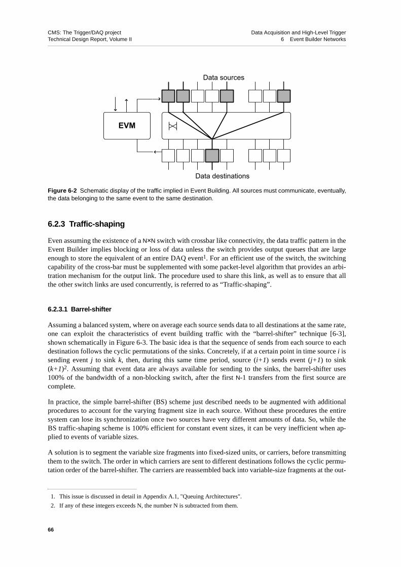
CMS: The Trigger/DAQ project Data Acquisition and High-Level TriggerTechnical Design Report, Volume II 6 Event Builder Networks
6.2.3 Traffic-shaping
Even assuming the existence of a N×N switch with crossbar like connectivity, the data traffic pattern in theEvent Builder implies blocking or loss of data unless the switch provides output queues that are largeenough to store the equivalent of an entire DAQ event1. For an efficient use of the switch, the switchingcapability of the cross-bar must be supplemented with some packet-level algorithm that provides an arbi-tration mechanism for the output link. The procedure used to share this link, as well as to ensure that allthe other switch links are used concurrently, is referred to as “Traffic-shaping”.
6.2.3.1 Barrel-shifter
Assuming a balanced system, where on average each source sends data to all destinations at the same rate,one can exploit the characteristics of event building traffic with the “barrel-shifter” technique [6-3],shown schematically in Figure 6-3. The basic idea is that the sequence of sends from each source to eachdestination follows the cyclic permutations of the sinks. Concretely, if at a certain point in time source i issending event j to sink k, then, during this same time period, source (i+1) sends event (j+1) to sink(k+1)2. Assuming that event data are always available for sending to the sinks, the barrel-shifter uses100% of the bandwidth of a non-blocking switch, after the first N-1 transfers from the first source arecomplete.
In practice, the simple barrel-shifter (BS) scheme just described needs to be augmented with additionalprocedures to account for the varying fragment size in each source. Without these procedures the entiresystem can lose its synchronization once two sources have very different amounts of data. So, while theBS traffic-shaping scheme is 100% efficient for constant event sizes, it can be very inefficient when ap-plied to events of variable sizes.
A solution is to segment the variable size fragments into fixed-sized units, or carriers, before transmittingthem to the switch. The order in which carriers are sent to different destinations follows the cyclic permu-tation order of the barrel-shifter. The carriers are reassembled back into variable-size fragments at the out-
Figure 6-2 Schematic display of the traffic implied in Event Building. All sources must communicate, eventually,the data belonging to the same event to the same destination.
1. This issue is discussed in detail in Appendix A.1, "Queuing Architectures".
2. If any of these integers exceeds N, the number N is subtracted from them.
Data sources
Data destinations
EVM
66

CMS: The Trigger/DAQ project Data Acquisition and High-Level TriggerTechnical Design Report, Volume II 6 Event Builder Networks
put. This is equivalent to having source-driven Time-Division Multiplexing of the data to the varioussinks.
In the simplest case, fragments are split into carriers without packing data from two adjacent fragmentsinto the same carrier, i.e. the end of the first fragment and the beginning of the next. This can neverthelessbe reasonably efficient, provided the carrier size is small compared to the typical fragment size. If, on theother hand, the carrier size is relatively large compared to the fragment size, high efficiency can only beobtained by packing data from different fragments into a carrier. The disadvantage here is that the seg-mentation and reassembly process are more complicated.
6.2.3.2 Destination-driven Traffic-shaping
In this scheme, one relies on the destinations to send their requests for data to the sources in an order thatinherently avoids clashes. In practice, the RU Builder (described Section 6.5, "RU Builder") is driven bythe destinations, i.e. the Builder Units (BUs) which send requests for data only once they have buffersavailable. The simplest way to shape the traffic at the destination is to assume that the destination sends arequest to N RUs sequentially: a request to RU 1 (e.g. “send event 45”) is then followed by the actual datatransfer of the data from event 45, at which point the request for the same event is sent to RU 2, and so on,as shown in Figure 6-4. No data is transmitted into the BU link during the time the request message is sentand processed. This results in a reduced utilisation of the switching network, depending on the latency ofthe network and processing times.
Figure 6-3 Schematic of the Barrel-Shifter Traffic-Shaping scheme. During the first time slot, only source 1 issending data (to destination 1). During time slot 2, source 1 is sending to dest. 2, while source 2 is sending todestination 1. During time slot m, source 1 is sending to dest. m, source 2 to m-1 and so on. After N time slots(where N is the number of sources) all sources are sending data to mutually exclusive destinations.
Data sources Barrel shifter
Data sinks
Data flow Ti
me
Space
4
4
4
4
1
4
4
4
3
3
3
3
3
3
3
3
2
2
2
2
2
2
2
2
1
1
1
1
1
1
1
1
4
4
4
4
1
4
4
4
3
3
3
3
3
3
3
3
2
2
2
2
2
2
2
2
1
1
1
1
1
1
1
1
4
4
4
4
1
4
4
4
3
3
3
3
3
3
3
3
2
2
2
2
2
2
2
2
1
1
1
1
1
1
1
1
4
4
4
4
1
4
4
4
3
3
3
3
3
3
3
2
2
2
2
2
2
3
1
1
1
1
1
12
12
1
4
4
4
4
1
4
4
3
3
3
3
3
3
2
2
2
2
2
4
1
1
1
1
123
23
2
1
1
1
4
4
4
4
1
4
4
3
3
3
3
3
3
2
2
2
2
2
4
1
1
1
1
123
23
2
1
1
1
1 2 3
4 5 6
Steady state Steady state
67

CMS: The Trigger/DAQ project Data Acquisition and High-Level TriggerTechnical Design Report, Volume II 6 Event Builder Networks
6.2.3.3 Switch-based Traffic-shaping
In this scheme, the switch employed uses internal buffering as intermediate storage for data that cannotmomentarily be sent to the desired destination. If this buffering capability is large enough (e.g. greaterthan at least N events in the DAQ) then the sources need no knowledge of time-sharing among the desti-nations, and can simply send their data, assuming a cross-bar like connectivity, at any point in time.
Switches of this kind with a large number of 1 Gb/s ports already exist, albeit at relatively high cost. Nev-ertheless, the dependence of system performance, as well as its overall balance, on the internal character-istics of a specific proprietary switch is not a desirable feature. For this reason, this type oftraffic-shaping, while the easiest one to implement, remains the least attractive.
6.3 Network Technologies Considered for EVB Networks
This section discusses the network technologies, namely Switched Ethernet and Myrinet, which are con-sidered as possible implementations of the Event Builder networks. A comparison of the main features ofthese technologies is given in Table 6-1. The following subsections give a brief overview the two technol-ogies and describe their use in an Event Builder network.
6.3.1 Switched Ethernet
The term Ethernet refers to the family of LAN products covered by the IEEE 802.3 standard protocol. In-vented in 1976, Ethernet became a de-facto standard in 1980. Four data rates are currently defined for op-eration over twisted-pair cables or optical fiber (see Table 6-2).
Most of the LANs in use today are based on Ethernet. Ethernet started as a shared medium technology.Fast Ethernet introduced full duplex point to point links, which allowed a fast rise of data rates forswitched Ethernet. The success of this standard is attributed to its support of ever-higher data rate capabil-ities combined with high flexibility in network installations and full inter operability between productsfrom different manufacturers.
Figure 6-4 Principle of destination based traffic-shaping.
BU RU1 RU2
request
event data
BU input link active
68

CMS: The Trigger/DAQ project Data Acquisition and High-Level TriggerTechnical Design Report, Volume II 6 Event Builder Networks
6.3.1.1 Switched Ethernet Technology
An Ethernet network is composed of switching elements and NICs connected by point-to-point bidirec-tional links. Store-and-forward switches permit interconnection of links with different data rates. Packetsize is limited to 1500 bytes of data (plus header and trailer). The NIC is in general not programmable;but the switches are configurable and support extensions to the standard such as VLAN, which effectivelydivides a switch into several smaller switches.
The switches are in general non-blocking, i.e. the crossbar can support the aggregate rate of all the switchports; packets can still get lost because of capacity limitations in the store and forward memories. Flow
Table 6-1 Network technologies comparison.
Switched Ethernet Myrinet
focus Local Area Network cluster I/O
bandwidth 100 Mbps (Fast Ethernet)1 Gbps (Gigabit Ethernet)10 Gbps emerging
2.5 Gbps (8b/10b encodeda)
latency (MPI applicationb) 100 µs 10 µs
routing methodc destination-based source-based
switching algorithm store-and-forward (typically) wormhole
switch type shared memory (typically) crossbar
flow control Xon/Xoff pause frames (optional) link level Xon/Xoff
medium UTP5 up to 200 m, fiber
copper up to 3 m (SAN), fiber
MTU size 1500 bytes (user payload)jumbo frames (optional)
unlimited
multicast/broadcast yes no
processor on NIC typically not yes
market multi-vendor single vendor
a. Due to the 8b/10b encoding of the data the 2.5 Gbps baud rate results in a 2 Gbps effective bandwidth.
b. MPI (Message Passage Interface) is an industry standard employed widely in high-performance com-puting.
c. the routing method refers to whether the determination of the path to follow between source and des-tination is done at the source (source routing) or at each switching node along the way (destinationbased).
Table 6-2 Ethernet standard.
Bandwidth Standard Year of IEEE standardisation
10 Mbps 10 Base-T Ethernet 1991
100 Mbps Fast Ethernet 1995
1 Gbps Gigabit Ethernet 1999
10 Gbps 10 Gigabit Ethernet (fiber only) 2002
69

CMS: The Trigger/DAQ project Data Acquisition and High-Level TriggerTechnical Design Report, Volume II 6 Event Builder Networks
control is optional and is implemented through the use of pause frames generated by the Media AccessControl layer of the receiving NIC. Flow control is generally implemented between NIC and switch port,but not always through the switch back to the source NIC.
6.3.1.2 Switched Ethernet for Event Building
The bandwidth of Gigabit Ethernet is a factor two below the bandwidth required by a single data source(be it a FRL or a RU) in the Event Builder, so a Gigabit Ethernet solution requires at least two rails.10-Gigabit Ethernet is not an option at present as it only supports products for switch-to-switch communi-cation and not for the host-to-switch communication needed in the Event Builder.
The small frame size of Ethernet is a drawback because it increases the load on the hosts. A number ofcompanies have equipment that support bigger packet sizes, the so-called ‘Jumbo frames’. Althoughthese are not part of the IEEE standard they are becoming a de-facto standard supported by many Ethernetequipment manufacturers
The IEEE 802.3 physical layer does not guarantee error-free transmission. Packets may be lost if bufferspace is not available in any of the switches between the sender and the receiver. The protocols needed forevent building with Ethernet must be implemented on programmable hosts as long as the availability ofprogrammable NICs is not guaranteed1.
A lightweight application level protocol has been tested in a system with 64 hosts (see Section 6.5.2). Theperformance depends on the characteristics of the switch. A simulation of this setup is under way and it ishoped that this can be used to evaluate how the system scales with a doubling of the number of ports andhow performance depends on the memory size of the switch.
The TCP/IP protocol would be more convenient as it guarantees error free transmission over Ethernet, butit is demanding on the resources of the host. Preliminary results of event building using TCP/IP over Eth-ernet are given in Appendix B.3, "Gigabit Ethernet TCP/IP Test-benches". The basic conclusion is that, inspite of the overheads, it is now possible with TCP/IP to drive 2 GbE links near the full wire rate using a2 GHz Pentium-IV Xeon based PC. With the ever increasing PC performance, TCP/IP over GbE couldbecome an attractive candidate for the RU Builder over the next few years.
Overall, switched Ethernet is a valid candidate for the RU Builder, but it is not the leading candidate forthe switches in the FED Builder (See Section 6.4.3).
6.3.2 Myrinet
Myrinet is a high-speed interconnect for clusters, based on networking principles previously used in mas-sive parallel processors [6-4].
6.3.2.1 Myrinet Technology
A Myrinet network is composed of switching elements and network interface cards (NICs) connected bypoint-to-point bidirectional links. The effective link speed is currently 2 Gb/s. The core of the switchingchip is a pipelined 16-port crossbar that supports non-blocking wormhole (also known as cut-through)
1. As an example, some programmable NICs that were available at the time of the prototypes, described later in thischapter, have had their software support withdrawn.
70

CMS: The Trigger/DAQ project Data Acquisition and High-Level TriggerTechnical Design Report, Volume II 6 Event Builder Networks
routing of packets. Packets can be of arbitrary size. Network link-level flow control guarantees the deliv-ery of packets at the expense of an increased potential for blocking in the switches. The NIC has a RISCprocessor whose firmware can be programmed to interact directly with the host processor for low-latencycommunications and with the network links to send, receive and buffer packets.
Myrinet is specified at the data link and physical level as an ANSI standard [6-5]. Myrinet products aremanufactured by Myricom [6-6]. Details can be found in Appendix A.2, "Myrinet Technology and Prod-ucts".
6.3.2.2 Myrinet for Event Building
The implemention of the Event Builder networks using Myrinet has numerous attractive features:
• large network fabrics can be constructed with ease
• data packets can be of arbitrary size
• there is no packet loss inside the switching fabric, while the bit error rate is very low
• the RISC processor on the NIC is programmable. This feature can be useful for implementing traf-fic-shaping, event building, or for optimized protocols. This is particularly relevant if the host isnot a general-purpose fully programmable CPU but an FPGA-based device.
Even with a lossless switching fabric data can get lost due to overruns in the receiver buffers on the NICor on the host. These losses can be avoided by flow control at the application level or by propagatingpressure from the receiver host and NIC backwards to the sender. With a bit error rate below 10-15, dis-carding those packets will lead to an insignificant efficiency loss and therefore there is no need for amechanism for the recovery from such errors on an event-by-event basis. Only an error detection mecha-nism is still required.
A Myrinet network is essentially an input-queued switching fabric (see Appendix A, "Overview ofSwitching Techniques and Technologies"). Hence, depending on the traffic pattern, the throughput can belimited by head-of-line blocking. For random traffic, the maximum utilisation has an asymptotic theoreti-cal limit of 59% for a single-stage network. For multi-stage networks the maximum utilisation is furtherreduced, as there is essentially no buffering in the switches.
Event building can be more demanding than random traffic since it creates a high degree of congestion atthe switch output nodes. Simulation studies of event building with variable-size fragments show that, de-pending on details of the fragment size distributions and the number of stages, a ~50% utilisation of thebisection bandwidth is obtained. These studies are detailed in Appendix B.1, "EVB Performance withMyrinet Switches".On the other hand, a 100% utilisation of the network can be reached, in principle, withbarrel-shifter traffic-shaping, assuming balanced inputs.
Overall, Myrinet is a valid candidate for the RU Builder switches as well as the FED Builder switches.
6.4 FED Builder
This section discusses the first stage of the Event Builder; the FED Builder. It starts with a brief review ofits main functions. A possible configuration of the FED Builder based on the expected data rates from allCMS subdetectors is outlined. This is followed by a discussion on the network implementations for theFED Builder. Implementations with Ethernet and with Myrinet are considered. Measurements made on
71

CMS: The Trigger/DAQ project Data Acquisition and High-Level TriggerTechnical Design Report, Volume II 6 Event Builder Networks
prototypes and performance estimates made through simulation show that the networking requirements ofthe FED Builder can be met with the networking technology available in 2003.
6.4.1 Introduction
The main functions of the FED Builder are (see Section 4.2)
• to read the FED data and act as a buffer to smooth the bursty arrival of data.
• to assemble event fragments of variable sizes from some 600 FEDs into 64 super-fragments ofroughly equal size (16 kB each)
• to multiplex these super-fragments on an event-by-event basis between N (N≤8) RU Builders, i.e.the second stage of the Event Builder.
These functions are achieved by 64 FED Builder switches, each with 8 input and 8 output ports. The inputports are connected to the FRL, whereas the output ports are connected to the RUI.
A 8×8 switch is the current design choice for the FED Builder, but other configurations can be imple-mented easily as well. In particular, a 16×8 switch configuration can be used to merge more FRLs as analternative to merging low rate FEDs in the FRL.
6.4.2 FED Builder Configuration
At the time of writing, it is foreseen that the CMS readout will contain a total of ~630 FEDs which areconcentrated into ~460 FRLs in order to reduce the number of EVB switch inputs. The details of thisscheme are described in Section 7.2.3, "Sub-detector Readout Parameters". The FRLs are the inputs ofthe FED Builders. A possible configuration of the FED Builder is given in Table 6-3. The breakdown forthe tracker-silicon detector will be discussed in more detail below. The assignment of FEDs to FEDBuilder (FEDB) switches takes into account the following considerations:
• FEDs providing a relatively small volume of data can be concentrated into a single FRL. It is as-sumed that up to 2 FEDs can be merged. Merging by the FRLs is used for the Silicon-TrackerFEDs.
• Detectors are not mixed on the same FEDB switch, so that they can be operated independently
• FEDs (and hence FRLs) with a relatively high data volume are combined with FEDs with a rela-tively small data volume on the same switch in order to achieve super-fragments of about equalsize. This applies to the tracker-silicon.
• Partitioning considerations add the constraint that FEDs from different TTC partitions may not bemixed on the same FEDB switch (see Section 4.4.2, "DAQ Partitioning"). This restriction holdsfor RU Builder partitioning. It ensures that no FEDB switch and associated RUI and RU will haveto be shared between two DAQ partitions which always follow TTC partition boundaries. Thepresent assignment takes partition constraints only into account for the tracker-pixel and track-er-silicon detectors. Strict adherence to these rules would require a substantial number of addition-al FED Builders for the other detectors with a small number of FEDs and a relatively large numberof TTC partitions. However, it is probably acceptable in practice, that the DAQ partitioning ismore restrictive than the constraints imposed by the TTC partitioning.
About half of the total data rate is expected to come from the tracker-silicon detector. The data rate ex-pected from each individual FED of the silicon tracker has been estimated (see [6-7]). FED-to-FED vari-
72

CMS: The Trigger/DAQ project Data Acquisition and High-Level TriggerTechnical Design Report, Volume II 6 Event Builder Networks
ations are about a factor of three. The expected data rate is estimated to have an uncertainty of about 40%.A proposal on which FED data streams should be merged using the FRLs is summarised in Table 6-4. Apossible assignment of FED Builders to these FRLs is given in Table 6-5. The resulting average su-per-fragment size varies between 6.5 and 9.3 kB. This assignment provides reasonably balanced inputs tothe second stage of the EVB and the value is well below the nominal 16 kB size. This margin is probablynecessary in view of the uncertainty on the data rates.
The current design choice is to use 8×8 switches in the FED Builder and 64×64 switches in the RU Build-er. Hence, there are 63 FED Builders available, if one port of the RU Builder input switch is reserved forconnection to the Event Manager. The current assignment uses 63 FED Builders, which leaves one freefor contingency. However, the architecture is flexible, because more aggressive merging can be providedat the FRL level and by using N×8 switches for the FED Builder.
Table 6-3 FED Builder configuration.
Detector TTC partition # of FEDs FEDs per FRL # of FRLs # of FEDBs
Tracker - pixelbarrel 32 1 32 4
both endcaps 6 1 6 1
Tracker - silicon
inner 114 1 (54) or 2 (30) 84 11
outer 134 1 (2) or 2 (66) 68 9
endcap+ 96 1 (24) or 2 (36) 60 8
endcap- 96 1 (24) or 2 (36) 60 8
Preshower 47 1 47 6
ECAL 54 1 54 7
HCAL 32 1 32 4
Muon CSC 8 1 8 1
Muon RPC 6 1 6 1
Muon DT 5 1 5 1
Triggera 6 1 6 1
Total 636 468 63
a. Trigger comprises 4 FEDs for global trigger, and 1 FED for each of the Muon track finders (CSCand DT).
73

CMS: The Trigger/DAQ project Data Acquisition and High-Level TriggerTechnical Design Report, Volume II 6 Event Builder Networks
Table 6-4 Estimated data rate from the FEDs of the tracker silicon-detector and a pro-posed FED-FRL merging (from [6-7]). The FRLs have been sub-divided into categoriesdepending on the number of FEDs they read from each layera. An estimated average sizeof the fragments is also included. The sizes are for high luminosity pp collisions with FEDzero-suppression. Note that the numbers are for one endcap only.
FRL category
# of FRLs of this
categoryReads FEDs from layers
average size (B)
inner
1 24 TIB-1 1030
2 16 TIB(2+2) 1380
3 12 TIB(3+4) 1250
4 2 TIB(4+4) 1040
10 10 TID1 810
11 10 TID2 810
12 10 TID3 810
outer
5 22 TOB(1+5) 1080
6 24 TOB(2+6) 960
7 14 TOB(3+4) 910
8 2 TOB4 410
9 6 TOB(5+6) 620
each endcap
13 32 TEC(1-3)+TEC(4-6) 1380
14 4 TEC(1-3)+TEC(1-3) 1320
15 16 TEC(7-8) 1010
16 8 TEC9 1040
a. The tracker consists of 20 barrel layers and 24 end-cap disks. The inner and outer barrellayers are named TIB1-4 and TOB1-6, respectively. The end-cap disks consist of 3mini-disks named TID1-3 and 9 larger disks named TEC1-9.
74

CMS: The Trigger/DAQ project Data Acquisition and High-Level TriggerTechnical Design Report, Volume II 6 Event Builder Networks
6.4.3 FED Builder implementation with Ethernet
Ethernet has been considered for the FED Builder switch, however a full prototyping effort has not beenlaunched because of the following shortcomings of Ethernet with respect to Myrinet for this application:
• Bandwidth. The bandwidth limitation of Gigabit Ethernet would require a three-rail implementa-tion.
• NICs. Gigabit Ethernet NICs supporting this number of rails are starting to become available, butare not, at least currently, programmable.
• FRL complexity. Ethernet NICs are not programmable, so the FED Builder protocol would have tobe implemented in the FPGA of the FRL. The current FRL design uses a simple FIFO buffer be-tween FED input and NIC output, whereas Ethernet NICs typically assume packet buffers to be inrandom access memory.
• Ethernet does not provide a lossless packet transport. (Packets may be lost if the switch momentar-ily has insufficient buffer space). A transmission protocol that includes detection and retransmis-sion of lost packets is more complex and difficult to implement in FPGAs. This drawback does nothold when using switches implementing flow control.
• In order to implement back pressure from RU to FED, we need to restrict ourselves to switcheswhich implement flow control.
Table 6-5 FED Builder configuration for the tracker-silicon detector. The FED Builders (FEDB) have beensub-divided into categories depending on the FRLs connected to their 8 input ports. As an example, the first rowmeans that there are 4 FED Builders of category 1, where each FED Builder has 2 inputs connected to FRLs ofFRL category 1, 2 inputs connected to category 2, 1 input connected to category 3, 2 inputs connected to cate-gory 10 and 1 input port is free. The estimated average size of the resulting super-fragments is also included.The sizes are for high luminosity pp collisions with FED zero-suppression.
FEDB category
# of FEDBs in this
category
FEDB inputs from FRL category
average super-
fragment size (B)
inner
1 4 2*FRL-1 + 2*FRL-2 + 1*FRL-3 + 2*FRL-10 + 1 free 7690
2 1 2*FRL-1 + 2*FRL-2 + 1*FRL-3 + 2*FRL-10 + 1*FRL-11 8500
3 1 2*FRL-1 + 1*FRL-2 + 2*FRL-3 + 3*FRL-11 8370
4 2 2*FRL-1 + 1*FRL-2 + 1*FRL-3 + 1*FRL-4+ 3*FRL-11 8160
5 2 3*FRL-1 + 1*FRL-2 + 1*FRL-3 + 3*FRL-12 8150
6 1 2*FRL-1 + 1*FRL-2 + 1*FRL-3 + 4*FRL-12 7930
outer
7 3 8*FRL-6 7680
8 2 7*FRL-7 + 1*FRL-8 6780
9 3 5*FRL-5 + 2*FRL-9 + 1 free 6640
10 1 7*FRL-5 + 1 free 7560
each endcap11 4 4*FRL-13 + 1*FRL-14 + 2*FRL-16 + 1 free 8920
12 4 4*FRL-13 + 4*FRL-15 9560
75

CMS: The Trigger/DAQ project Data Acquisition and High-Level TriggerTechnical Design Report, Volume II 6 Event Builder Networks
• RU load. Without programmable NICs, the super-fragments would have to be built by the RU,which requires packet chaining or data copying in the RU memory. This is critical, because I/O andmemory bandwidth is currently the most severe bottleneck in the use of PCs for implementation ofthe RU.
The advent of programmable multi-rail Gigabit Ethernet NICs or programmable 10 Gigabit NICs wouldremove most of these obstacles.
6.4.4 FED Builder Implementation with Myrinet
Myrinet supports reliable transport with back pressure at the hardware level, the NICs are programmableand have sufficient memory to smooth bursty arrival of data from the FRL. Myrinet supports a bandwidthper port of 2 Gb/s (or 250 MB/s). The switch utilisation will be roughly 50% when transporting variablesize fragments (as discussed above in Section 6.3.2.2). The switch capacity therefore has to be doubled toabsorb an average of 200 MB/s per port. LANai10 based NICs with two links per NIC are expected to beavailable in 2003. These can be used to construct a two-rail network, where each link of the NIC is con-nected to two independent 8×8 crossbar switches (see Figure 6-5).
The Clos-128 switches from Myricom provide 128 external ports with a three stage Clos network using8×8 crossbars. It is therefore possible to configure these switches either as eight 8×8 switches or as four16×8 switches by just reprogramming the routes of the wormhole packets. This could be used to enablethe FED Builder to provide data concentration.
The FRLs with their NICs are located in the cavern close to the FED crates, whereas the switches are lo-cated at the surface in the DAQ room. The Myrinet links from the FRL NICs to the switches are standardoptical fibers (multi mode 50/125 mm diameter) with a maximum length of 200 m.
Figure 6-5 FED Builder based on Myrinet.
8 RUI systems
FED
Bui
lder
(FB)
8 FRL systems
LANai10 2XPNetwork Interface Card (NIC)
76

CMS: The Trigger/DAQ project Data Acquisition and High-Level TriggerTechnical Design Report, Volume II 6 Event Builder Networks
6.4.4.1 Design
As described in Section 4.2, "FED Builder" the NICs at the FRL side correspond to the FED Builder In-puts (FBI) and the NICs at the RU side correspond to the Readout Unit Inputs (RUI).
The FBI is programmed to read event fragments from the FRL at the highest possible rate and buffer themin its memory in FIFO order. Event fragments in this buffer are transmitted to an output port at the ratethat can be accepted by the link. The destination port for each fragment is derived by the FBI from thefragment event number. A lookup table addressed through the lowest 8 bits of the event number is usedfor this purpose. In the simplest case event number modulo 8 is used, but more complex algorithms can bestored in the lookup table.
The RUI, acts as a small Event Builder, concatenating event fragments with the same event number fromall the FBIs and building super-fragments. The super-fragments may become available out of sequencesince fragments arrive by two different switches (rails). It is the task of the RUI program to deliver the su-per-fragments to the RU in order of increasing event number. The RUI builds super-fragments directly inthe memory of its host RU by using DMA chaining of all the fragments from one event as soon as theyare all ready in the RUI memory.
The buffer memories in the FBI and RUI are organised in fixed sized blocks. All transfers of event frag-ments from the FRL to the FBI, and from FBI to the RUI are performed in units of blocks. The blocksizeis called the FEDB block size. The FBI sends all blocks belonging to one fragment along the same railthrough the FED Builder switch so that all blocks belonging to a fragment arrive in sequential order at theRUI. The buffer memory in the RU is also organised in fixed size blocks, but not necessarily of the samesize as in the FED Builder.
The FBIs send the fragment blocks asynchronously with respect to each other. Hence, a deadlock situa-tion can occur in the event building process in the RUI if the amount of buffer memory is not sufficient tostore all the data corresponding to the range of triggers being processed. In order to avoid this, it is fore-seen to implement a credit scheme, where the number of blocks sent by the FBI is limited by the creditsreceived from the RUI.
6.4.4.2 Error Handling
The Myrinet switching fabric does not lose packets and the credit scheme protocol ensures that the receiv-ing NIC (RUI) has buffer space available for incoming packets. Therefore, packets will not be lost in theFED Builder. However, packets can be corrupted due to transmission errors. These errors are detected viaa CRC. All packets with CRC errors are simply dropped, but this leads to an insignificant event loss prob-ability of about 10-8 with a Myrinet bit error rate below 10-15 and an event size of 107 bits.
It is foreseen to impose an upper limit on the fragment size in order to protect against pathological cases.If the FBI receives a fragment which is too big, it will read the full fragment from the FRL, discard thedata and insert an error flag in the header. It will then transmit only the fragment header to the RUI.
The RUI has a limited buffer space and can not wait indefinitely for data from the FEDs. The NIC releas-es the incomplete event for transfer to the RU if data from one of the FEDs does not arrive within a prede-fined time limit.
6.4.4.3 Test-benches
Different aspects of the FED Builder have been studied using two test-benches, both based on LANai9.
77
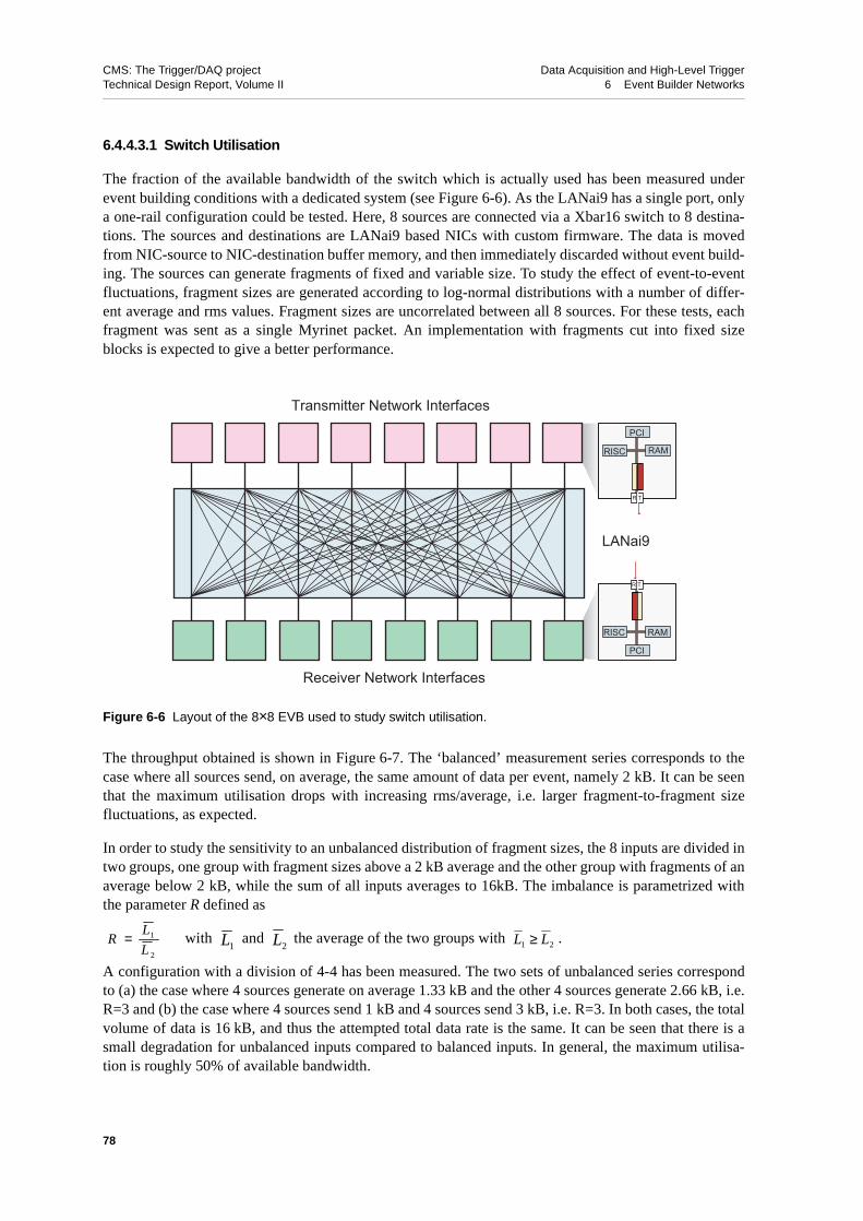
CMS: The Trigger/DAQ project Data Acquisition and High-Level TriggerTechnical Design Report, Volume II 6 Event Builder Networks
6.4.4.3.1 Switch Utilisation
The fraction of the available bandwidth of the switch which is actually used has been measured underevent building conditions with a dedicated system (see Figure 6-6). As the LANai9 has a single port, onlya one-rail configuration could be tested. Here, 8 sources are connected via a Xbar16 switch to 8 destina-tions. The sources and destinations are LANai9 based NICs with custom firmware. The data is movedfrom NIC-source to NIC-destination buffer memory, and then immediately discarded without event build-ing. The sources can generate fragments of fixed and variable size. To study the effect of event-to-eventfluctuations, fragment sizes are generated according to log-normal distributions with a number of differ-ent average and rms values. Fragment sizes are uncorrelated between all 8 sources. For these tests, eachfragment was sent as a single Myrinet packet. An implementation with fragments cut into fixed sizeblocks is expected to give a better performance.
The throughput obtained is shown in Figure 6-7. The ‘balanced’ measurement series corresponds to thecase where all sources send, on average, the same amount of data per event, namely 2 kB. It can be seenthat the maximum utilisation drops with increasing rms/average, i.e. larger fragment-to-fragment sizefluctuations, as expected.
In order to study the sensitivity to an unbalanced distribution of fragment sizes, the 8 inputs are divided intwo groups, one group with fragment sizes above a 2 kB average and the other group with fragments of anaverage below 2 kB, while the sum of all inputs averages to 16kB. The imbalance is parametrized withthe parameter R defined as
with and the average of the two groups with .
A configuration with a division of 4-4 has been measured. The two sets of unbalanced series correspondto (a) the case where 4 sources generate on average 1.33 kB and the other 4 sources generate 2.66 kB, i.e.R=3 and (b) the case where 4 sources send 1 kB and 4 sources send 3 kB, i.e. R=3. In both cases, the totalvolume of data is 16 kB, and thus the attempted total data rate is the same. It can be seen that there is asmall degradation for unbalanced inputs compared to balanced inputs. In general, the maximum utilisa-tion is roughly 50% of available bandwidth.
Figure 6-6 Layout of the 8×8 EVB used to study switch utilisation.
LANai9
RISC
PCI
RAM
TR
RISC
PCI
RAM
TR
Transmitter Network Interfaces
Receiver Network Interfaces
2
1
L
LR =
1L 2L 21 LL ≥
78
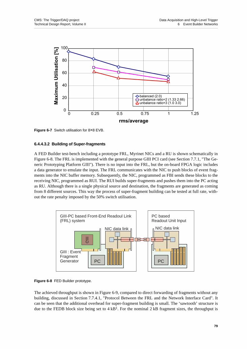
CMS: The Trigger/DAQ project Data Acquisition and High-Level TriggerTechnical Design Report, Volume II 6 Event Builder Networks
6.4.4.3.2 Building of Super-fragments
A FED Builder test-bench including a prototype FRL, Myrinet NICs and a RU is shown schematically inFigure 6-8. The FRL is implemented with the general purpose GIII PCI card (see Section 7.7.1, "The Ge-neric Prototyping Platform GIII"). There is no input into the FRL, but the on-board FPGA logic includesa data generator to emulate the input. The FRL communicates with the NIC to push blocks of event frag-ments into the NIC buffer memory. Subsequently, the NIC, programmed as FBI sends these blocks to thereceiving NIC, programmed as RUI. The RUI builds super-fragments and pushes them into the PC actingas RU. Although there is a single physical source and destination, the fragments are generated as comingfrom 8 different sources. This way the process of super-fragment building can be tested at full rate, with-out the rate penalty imposed by the 50% switch utilisation.
The achieved throughput is shown in Figure 6-9, compared to direct forwarding of fragments without anybuilding, discussed in Section 7.7.4.1, "Protocol Between the FRL and the Network Interface Card". Itcan be seen that the additional overhead for super-fragment building is small. The ‘sawtooth’ structure isdue to the FEDB block size being set to 4 kB1. For the nominal 2 kB fragment sizes, the throughput is
Figure 6-7 Switch utilisation for 8×8 EVB.
Figure 6-8 FED Builder prototype.
0
20
40
60
80
100
0 0.25 0.5 0.75 1 1.25
rms/average
Max
imum
Util
isat
ion
[%]
balanced (2.0)unbalance ratio=2 (1.33 2.66)unbalance ratio=3 (1.0 3.0)
PC PC
GIII
GIII-PC based Front-End Readoul Link (FRL) system
PC based Readout Unit Input
GIII : EventFragment Generator
NIC data linkNIC data link
79

CMS: The Trigger/DAQ project Data Acquisition and High-Level TriggerTechnical Design Report, Volume II 6 Event Builder Networks
230 MB/s, corresponding to a trigger rate of 115 kHz. With a super-fragment size of 16 kB at the outputof the FED Builder, this corresponds to building super-fragments at the rate of 14 kHz. It should be notedthat this prototype version does not yet implement a credit scheme and error detection.
6.4.4.4 Simulation
A detailed simulation model of the Event Builder complex has been implemented and is described inAppendix B.4, "Simulation of Myrinet Event Builder". In the following, results of the simulation arecompared to data obtained with the FED Builder prototype described above. A prediction is made for theperformance of the FED Builder based on LANai10 hardware and a two-rail network.
The data sizes in the CMS DAQ system are approximated by a log-normal distribution. However, it islikely, that the different data sources will be correlated and that the distributions will be different for dif-ferent sources. To study the sensitivity of the throughput to these issues, the correlation of fragment sizesbetween data sources as well as unbalanced input distributions are studied. In rare cases a very big frag-ment might be emitted by one data source. The impact of these “jumbo-fragments” on the system per-formance is also tested.
6.4.4.4.1 Comparison of the 8×8 EVB with Test-bench Measurements
The results of the simulation for the switch utilisation of the 8×8 EVB are compared with the measure-ments presented in Section 6.4.4.3.1 in Figure 6-10. Reasonable agreement is obtained. The asymptoticvalue for large rms/average and imbalance ratio of 3 is about 45% (not shown).
6.4.4.4.2 Prediction for Two-rail FED Builder Based on LANai10
The performance of the FED Builder based on a two-rail LANai10 configuration has been estimated. Thesystem operates in saturation mode, where the data sources always assume an event available. The
1. The RU blocksize was set to 80 kB, i.e. larger than the maximum super-fragment tested.
Figure 6-9 FED Builder prototype. Throughput versus fragment size.
0
50
100
150
200
250
300
0 1000 2000 3000 4000 5000 6000 7000 8000 9000 10000
FED fragment size [Bytes]
Thro
ughp
ut [M
B/s
]
Myrinet link 2 Gbpsforward fragment segmentssuper fragment building
80
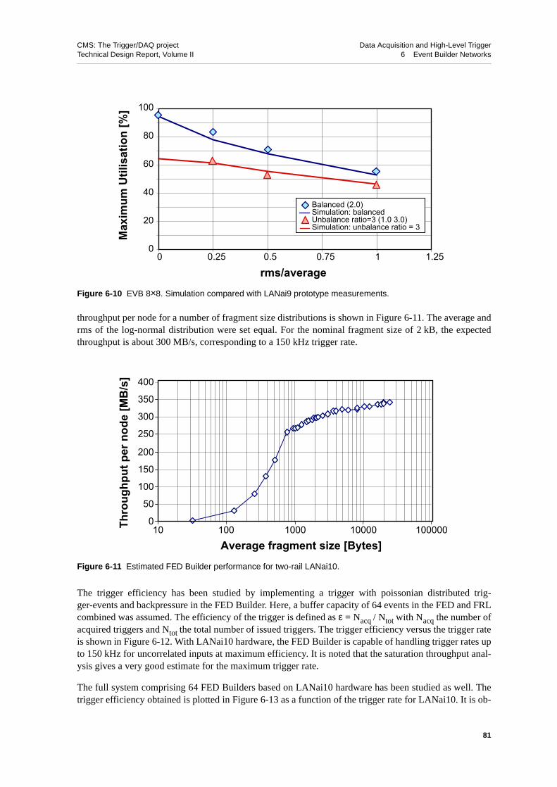
CMS: The Trigger/DAQ project Data Acquisition and High-Level TriggerTechnical Design Report, Volume II 6 Event Builder Networks
throughput per node for a number of fragment size distributions is shown in Figure 6-11. The average andrms of the log-normal distribution were set equal. For the nominal fragment size of 2 kB, the expectedthroughput is about 300 MB/s, corresponding to a 150 kHz trigger rate.
The trigger efficiency has been studied by implementing a trigger with poissonian distributed trig-ger-events and backpressure in the FED Builder. Here, a buffer capacity of 64 events in the FED and FRLcombined was assumed. The efficiency of the trigger is defined as ε = Nacq / Ntot with Nacq the number ofacquired triggers and Ntot the total number of issued triggers. The trigger efficiency versus the trigger rateis shown in Figure 6-12. With LANai10 hardware, the FED Builder is capable of handling trigger rates upto 150 kHz for uncorrelated inputs at maximum efficiency. It is noted that the saturation throughput anal-ysis gives a very good estimate for the maximum trigger rate.
The full system comprising 64 FED Builders based on LANai10 hardware has been studied as well. Thetrigger efficiency obtained is plotted in Figure 6-13 as a function of the trigger rate for LANai10. It is ob-
Figure 6-10 EVB 8×8. Simulation compared with LANai9 prototype measurements.
Figure 6-11 Estimated FED Builder performance for two-rail LANai10.
0
20
40
60
80
100
0 0.25 0.5 0.75 1 1.25
rms/average
Max
imum
Util
isat
ion
[%]
Balanced (2.0)Simulation: balancedUnbalance ratio=3 (1.0 3.0)Simulation: unbalance ratio = 3
Thro
ughp
ut p
er n
ode
[MB
/s]
0
50
100
150
200
250
300
350
400
10 100 1000 10000 100000Average fragment size [Bytes]
81

CMS: The Trigger/DAQ project Data Acquisition and High-Level TriggerTechnical Design Report, Volume II 6 Event Builder Networks
served that up to a trigger rate of about 150 kHz the system is fully efficient. This shows that the maxi-mum trigger rate is not very sensitive to the number of FEDs in the system. The trigger efficiency of asystem of multiple FED Builders is not simply the product of the single FED Builder efficiencies, becausethe throttling of the trigger affects all FED Builders, and hence the systems are coupled. This can be un-derstood by the following argument. If one FED Builder is close to saturation and throttles the trigger, theother FED Builders will also receive no further triggers and hence empty their buffers as well.
6.4.4.4.3 Data Conditions
The fragment sizes in CMS will be correlated between the FEDs. Hence, it is important to study also theinfluence of correlated fragment sizes on the utilization of the switch. To this end, fragment sizes are gen-erated by a log-normal distribution with varying values for the linear correlation r between the different
Figure 6-12 Trigger efficiency versus trigger rate for one 8×8 FED Builder and a log-normal fragment size dis-tribution with average and rms set to 2 kB.
Figure 6-13 Trigger efficiency versus trigger rate for 64 8×8 FED Builders and a log-normal fragment size distri-bution with average and rms set to 2kB.
40
50
60
70
80
90
100
0 50 100 150 200Trigger rate [kHz]
LANai9LANai10
Trig
ger E
ffici
ency
[%]
40
50
60
70
80
90
100
0 50 100 150 200
Trigger rate [kHz]
Trig
ger E
ffici
ency
[%]
82

CMS: The Trigger/DAQ project Data Acquisition and High-Level TriggerTechnical Design Report, Volume II 6 Event Builder Networks
sources, where r is defined as
There are two limiting cases; a value of r=0 corresponds to uncorrelated sizes, the case considered so far,whereas with r=1 the sizes are identical in all sources (but with fragment-to-fragment fluctuations). Thethroughput as a function of r is shown in Figure 6-14. It is observed that the throughput is not sensitive tothe correlation between variable fragment sizes for both LANai9 and LANai10 hardware.
The sensitivity to an unbalanced distribution of fragment sizes has been studied for two configurations; adivision of 4-4 and a division of 1-7. The throughput has been simulated within a range of 1 < R < 6 forLANai9 and LANai10 hardware (see Figure 6-15).
Figure 6-14 Throughput as function of correlation parameter between inputs.
Figure 6-15 The simulated throughput of an 8×8 FED Builder as a function of the imbalance parameter R.
SS
Sr
yyxx
xy= ∑ −−= ))(( yyxxSxywith
Thro
ughp
ut p
er n
ode
[MB
/s]
0
50
100
150
200
250
300
0 0.2 0.4 0.6 0.8 1Correlation r
LANai9LANai10
0
50
100
150
200
250
300
0.9 1.9 2.9 3.9 4.9 5.9
Imbalance R
Thro
ughp
ut p
er n
ode
[MB
/s]
LANai10 4-4LANai10 1-7LANai9 4-4LANai9 1-7
83

CMS: The Trigger/DAQ project Data Acquisition and High-Level TriggerTechnical Design Report, Volume II 6 Event Builder Networks
In case of the 4-4 division, it is found that for reasonable values of R up to 3 the utilisation drops from60% for R=1 to 40% for R=3 (two-rail LANai10). An imbalance of R=3, corresponds to =3 kB and
=1 kB. For the 1-7 division, an imbalance of R=1.5 is acceptable, corresponding to =2.9 kB and=1.9 kB. In conclusion, for super-fragment sizes of 16 kB on average, a throughput of 200 MB/s per
node can be achieved, provided no source exceeds 3 kB fragment size on average (or 300 MB/s). Thecase when one FRL sends a fragment of abnormally large size may occur and the DAQ system must han-dle such cases. The simulation shows, that the DAQ system can handle these events with negligible deg-radation of performance because the fragments are transmitted in blocks (see Appendix B.4 for details).
6.5 RU Builder
This section discusses the second stage of the Event Builder; the RU Builder. Two possible implementa-tions are outlined; with Ethernet and Myrinet. Measurements made on test-benches and performance esti-mates made through simulation show that the networking requirements of the RU Builder can be met withthe networking technology available today.
6.5.1 Introduction
The function of the RU Builder (see Section 4.3, "RU Builder") is to assemble the event super-fragmentsfrom the 64 FED Builders into full events ready for processing in the filter farm. The main functional ele-ments of the RU Builder are:
• 64 Readout Units (RUs) with large buffers that serve to de-couple the flow of data out of the FEDBuilders from the flow of data into the RU Builder.
• 64 Builder Units (BUs) where full events are assembled and then sent off to the filter farm
• 1 Event Manager, whose primary function is to adapt the traffic in the RU Builder to the through-put capacity of the BUs and their associated filter farms. It consists of two closely coupled units,the Readout Manager (RM) and the Builder Manager (BM)
• 3 logical networks connecting the storage and processing elements
a. Builder Control Network (BCN). Connects all units in the system and whose main functionis to enable the flow of control information.
b. Builder Data Network (BDN). The high-throughput network used for the transfer of eventdata. It connects all the RUs to all the BUs.
c. Readout Control Network (RCN).Connects the Event Manager to all the RUs. It serves todistribute common Readout information to all the RUs
Each RU Builder must be able to sustain an event rate of up to 12.5 kHz. which corresponds to a datathroughput of 12.5 kHz ⋅ 16 kB = 200 MB/s for each RU and BU node.
1L2L 1L
2L
84

CMS: The Trigger/DAQ project Data Acquisition and High-Level TriggerTechnical Design Report, Volume II 6 Event Builder Networks
6.5.2 RU Builder Implementation with Ethernet
6.5.2.1 Design
The required 200 MB/s sustained throughput per node can be reached with a two-rail Gigabit Ethernetconfiguration and an effective throughput above 80% of the wire speed. Hence, each node accommodatestwo ports (either by using two NICs or by using a single NIC with two ports), each connected to one ofthe two rails. The network for each rail is provided by a 128 port switch. As an alternative to a singlechassis 128 port switch, the switch network can be provided by a multi-stage arrangement of switcheswith a smaller number of ports in one chassis.
An important design choice concerns the communication protocol. In particular whether to use EthernetLayer-2 frames or a reliable high level protocol, such as TCP/IP. A comparison of their merits is given inTable 6-6.
As will be shown in this section, it is feasible to operate an EVB close to the wire speed, using Layer-2frames. However, this necessitates traffic-shaping and a recovery protocol at the application level. Use ofTCP/IP is more demanding on host resources and the scaling properties for event builder traffic at highload are still unknown. Preliminary results with TCP/IP are given in Appendix B.3, "Gigabit EthernetTCP/IP Test-benches" and are summarised below.
6.5.2.2 EVB Protocol for Layer-2 Frames
Experience so far has shown that, typically, large switches do not implement endpoint-to-endpoint flowcontrol through the switch. Hence, packets can get lost due to congestion. With traffic-shaping the con-gestion can be reduced.
The event building protocol has been presented in general terms in Section 5.3.2.1, "Event Flow Proto-cols". The specific protocol used here is shown in Figure 6-16. To reduce congestion at the output ports,each BU requests event fragments from each RU sequentially. This is similar to the destination based traf-fic-shaping, discussed in Section 6.2.3.2. In order to use the links efficiently, several events have to bebuilt concurrently.
Table 6-6 Communication protocol comparison for Ethernet Event Builder.
Layer-2 frames TCP/IP
host computer or more basic (e.g. FPGA) computer
reliability packet loss if congestion reliable
zero-copy yes no
host CPU usage low high a
a. according to an empirical rule, 1 Hz of CPU is required per bps transmitted
EVB - traffic-shaping required maybe
EVB - recovery at application level built-in
EVB - latency medium high
85

CMS: The Trigger/DAQ project Data Acquisition and High-Level TriggerTechnical Design Report, Volume II 6 Event Builder Networks
The protocol has been augmented to recover from occasional packet loss exploiting the fact that the eventbuilding protocol is transaction based, where data are sent on request. The recovery is based on sequencenumbers, time-outs and a retry mechanism.
6.5.2.3 Test-bench Results for Layer-2 Frames
In the Event Builder test-bench, PCs are used to emulate BM, RUs and BUs. The BDN and BCN sharethe same physical Gigabit Ethernet network. The trigger is not emulated and the throughput measuredcorresponds to the saturation limit.
The application software running on the PCs implements the event building protocol discussed above, us-ing Layer-2 frames to transmit data. A library has been developed to send and receive Layer-2 framesfrom user space with zero-copy. This uses a modified Linux driver for the NIC.
6.5.2.3.1 One-rail Configuration
A 31×31 Event Builder based on Gigabit Ethernet has been set up. The nodes are 62 PCs emulating theRUs, BUs. In addition, one PC serves as the Event Manager BM. Details on the host configuration can befound in Table 6-7. The Gigabit Ethernet NIC of each host is connected to a FastIron-8000 switch from
Figure 6-16 Protocol for the Ethernet Event Builder with Layer-2 Frames.
Table 6-7 Configuration of the hosts used in the Gigabit Ethernet EVB test-bench.
Configuration element Equipment type
PC motherboard SuperMicro 370DLE with ServerWorks LE chipset
CPU Pentium-III, 750 MHz (RU and BM) or 1 GHz (BU)
PCIbus 64b/66MHz
Gigabit Ethernet NIC AceNIC from Alteon[6-9]
Operating System Linux 2.4
BU
BU
EVM
EVM
RU1RU1
RU2 RU3 RUn
allocate
confirm
sendcache
86

CMS: The Trigger/DAQ project Data Acquisition and High-Level TriggerTechnical Design Report, Volume II 6 Event Builder Networks
Foundry Networks [6-8]. A fully populated FastIron switch comprises 8 modules with 8 Gigabit Ethernetports each, connected to a crosspoint backplane. Each module contains 2 MB of shared memory to bufferpackets. The bandwidth of the memory system and backplane is dimensioned such that the switch is fullynon-blocking. For our tests, the switch is configured such that each port can buffer up to 63 packets.
The throughput per node as a function of the fragment size is shown in Figure 6-17. Also shown is thecalculated maximum performance taking header sizes into account. The saw-tooth structure reflects theEthernet MTU size (1500 B) and is due to the fact that no aggregation of event fragments into packets isperformed. For fragment sizes up to roughly 8 kB, the throughput is reduced due to the packet handlingoverhead for control and data messages1. For medium fragment sizes in the range 8 kB-20 kB, close tomaximum performance is achieved. For fragment sizes larger than 20 kB, significant packet loss leads toinefficiency due to retransmission. Packet loss occurs because the BUs are building a number of events si-multaneously (set to 32) and it can happen that several RUs send instantaneously to the same destinationport, which will drop the packets if its buffer exceeds 63 packets. For the nominal (super)-fragment sizeof 16 kB the achieved throughput per node is 115 MB/s.
The performance for variable sizes has been studied by generating fragment sizes according to log-nor-mal distributions. The obtained performance for a number of rms values is presented in Figure 6-18. Itcan be seen that there is no considerable degradation with respect to the case of fixed size (rms=0).
The size of the Event Builder is varied from 3×3 to 31×31 in Figure 6-19 for the nominal case of variablesize fragments with an average of 16 kB and an rms of 8 kB. It can be seen that the throughput per nodescales with the size of the configuration.
6.5.2.3.2 Two-rail Configuration
A two-rail 15×15 EVB has been assembled by equipping all nodes with two NICs. Point-to-point meas-urements over two links show that the transmission rate is almost a factor two higher than with a single
1. A 15×15 setup based on different hardware and software with lower overhead is described in Appendix B.2.1,"Single-chassis Configuration for 15 x 15 Event Builder".
Figure 6-17 Throughput per node versus size for the 31×31 one-rail Gigabit Ethernet EVB.
0
20
40
60
80
100
120
140
100 1000 10000 100000Fragment Size [Bytes]
Thro
ughp
ut p
er N
ode
[(MB
/s]
link BW (1Gbps)calculationEVB 31x31 + BM
87

CMS: The Trigger/DAQ project Data Acquisition and High-Level TriggerTechnical Design Report, Volume II 6 Event Builder Networks
link, indicating that the transfers via the two NICs largely overlap. The resulting EVB performance fornominal fragment sizes is compared to the one-rail configuration in Figure 6-19. The throughput per nodescales with the size of the configuration and a value of 220 MB/s is achieved.
6.5.2.3.3 Multi-chassis Configuration
A multi-chassis configuration is an alternative to a single-chassis 128 port Gigabit Ethernet switch. Themulti-chassis option is investigated as a possible alternative whose cost-effectiveness will be evaluated atthe time of procurement. An Event Builder based on a multi chassis Ethernet switching network has beenstudied. For details see Appendix B.2.2, "A Multi-chassis Switching Network for a 48¥48 Event Build-er". With this configuration it is possible to build large switching networks out of smaller switches by in-
Figure 6-18 Throughput per node versus average size for the 31×31 one-rail Gigabit Ethernet EVB. The frag-ment sizes are generated according to log-normal distributions.
Figure 6-19 Throughput per node versus N×N for one-rail and two-rail Gigabit Ethernet EVB. The fragmentsizes are generated according to a log-normal distribution with an average of 16 kB and an rms of 8 kB.
0
20
40
60
80
100
120
140
100 1000 10000 100000
Fragment Size [Bytes]
Thro
ughp
ut p
er N
ode
[MB
/s]
link BW (1Gbps)EVB 31x31+BM - rms=0 (fixed)rms=1krms=8k
0
50
100
150
200
250
0 5 10 15 20 25 30
N for NxN EVB
Thro
ughp
ut p
er N
ode
[MB
/s]
link BW (1Gbps)2-rail EVB1-rail EVB
88

CMS: The Trigger/DAQ project Data Acquisition and High-Level TriggerTechnical Design Report, Volume II 6 Event Builder Networks
troducing an intermediate layer of switches. However the intermediate layer introduces multiple pathsbetween sources and destinations (RUs and BUs) and this is not allowed with Ethernet layer-2 switching.This problem is solved by using VLANs (IEEE 802.1q), supported by many Ethernet switches. VLANscan effectively divide a switch into multiple smaller independent switches. This can be used in the inter-mediate switch layer to split the multiple paths over separate networks.
6.5.2.4 Simulation for Layer-2 Frames
A simulation of the Ethernet-based Event Builder has been developed. The model includes the measuredoverhead of about 10 µs to transmit a packet. The switch model used is based on the FastIron architecture,including the internal buffer memory, output queues and high-performance crosspoint backplane. A com-parison of the results with the test-bench measurements is shown in Figure 6-20. Good agreement is ob-tained for fragment sizes up to 20 kB. The simulation will be extended to include recovery from packetloss.
6.5.2.5 Test-bench Results for TCP/IP
The TCP/IP option has been evaluated (see Appendix B.3, "Gigabit Ethernet TCP/IP Test-benches") us-ing the same test-bench. An EVB throughput per node of 75 MB/s has been obtained for variable frag-ment sizes with an average of 16 kB and an rms of 8 kB. The performance scales linearly with the size ofthe EVB configuration from 3×3 to 31×31. The throughput corresponds to 85% of the measured TCP/IPpoint-to-point throughput (88 MB/s). Due to this limitation of the host and/or NIC, the switch load is onlyabout 60%.
With recent hardware1 a point-to-point TCP/IP performance of 123 MB/s for a single link and 247 MB/sfor a dual link can be obtained using “Jumbo frames” (MTU size of 9000 B). Further study is required toinvestigate if a similar throughput can be achieved with an Event Builder based on such hardware.
Figure 6-20 Comparison with simulation.
1. PC based on a single 2 GHz Pentium-IV Xeon CPU.
Thro
ughp
ut p
er N
ode
[MB
/s]
0
20
40
60
80
100
120
140
100 1000 10000 100000Fragment Size [Bytes]
link BW (1Gbps)EVB 31x31 + BMsimulation
89

CMS: The Trigger/DAQ project Data Acquisition and High-Level TriggerTechnical Design Report, Volume II 6 Event Builder Networks
6.5.3 RU Builder Implementation with Myrinet.
6.5.3.1 Design
The RU Builder can be implemented with a one-rail configuration based on Myrinet-2000 (which has aneffective link speed of 2 Gb/s). A single Clos-128 switch provides the 128 ports of the 64×64 switchingnetwork. Shaping the traffic through the switch by operating it as a barrel-shifter is expected to yield closeto 100% utilisation. A system without traffic-shaping is easier to implement and operate and has lower la-tency, but, would yield only about 40% utilisation of the bisection bandwidth due to blocking in the net-work of multiple stages. Therefore, the barrel shifter system is the preferred solution.
A possible configuration of the 63×63 EVB is shown in Figure 6-21, where both BDN and BCN are usingthe same physical network. The ‘up-side’ of the 64×64 Clos-128 network connects to 63 RUs and theBM, whereas the ‘down-side’ connects to 63 BUs and one dummy node. The dummy node can potential-ly be used as BU (hence a 63×64 EVB) or as RM in a 63×63 EVB.
6.5.3.2 Barrel-shifter Implementation
As explained in Section 6.2.3.1, one can exploit the characteristics of the event building data traffic pat-tern to increase the system throughput by arranging the traffic through the switching network as a bar-rel-shifter.
Figure 6-21 Myrinet Clos-128 network used for 63×63 EVB + BM.
0,1,0
0,1,0
0,1,0
Ports
Ports
0-7
0-7
0,1,1
0,1,1
0,1,1
Ports
Ports
0-7
0-7
0,1,2
0,1,2
0,1,2
Ports
Ports
0-7
0-7
0,1,3
0,1,3
0,1,3
Ports
Ports
0-7
0-7
0,1,4
0,1,4
0,1,4
Ports
Ports
0-7
0-7
0,1,5
0,1,5
0,1,5
Ports
Ports
0-7
0-7
0,1,6
0,1,6
0,1,6
Ports
Ports
0-7
0-7
0,1,7
0,1,7
0,1,7
Ports
Ports
0-7
0-7
BM RU1 RU2 RU3 RU63
BU1 BU2 BU3 BU63
.......
.......
90

CMS: The Trigger/DAQ project Data Acquisition and High-Level TriggerTechnical Design Report, Volume II 6 Event Builder Networks
The basic idea of the Myrinet barrel-shifter is shown schematically in Figure 6-22. Each host on thesource side has a separate queue for each possible destination. The MCP program running on the NIC, cy-cles through all destinations, copies the data by DMA to the NIC buffer and sends the data in packets toall destinations in turn. The barrel shifter imposes fixed-sized carriers, but event fragments have variablesize. In order to deal with this, fragment data are treated as a continuous stream that is cut up into thefixed sized carriers of the barrel shifter. The NIC of the sender cuts the stream into the carriers, and theNIC of the receiver re-assembles the stream of fragment data from the carriers. This transport mechanismis true zero copy, as the host CPU is not used to copy the data. It also supports buffer-loaning.
In a ‘classic’ barrel-shifter, sources are synchronized to emit fixed size carriers in time slots in such a waythat no two sources send to the same destination during the same time slot and all sources regularly sendto all destinations in a cycle. A central controller is needed to synchronize the time sliced operation of allsources. Note that there is no central controller to apply an external synchronisation in this implementa-tion. Instead, it relies on the back-pressure flow control of Myrinet. After an initial synchronization steputilising the Myrinet network itself, all sources send through mutually exclusive paths to different desti-nations in a cycle. To keep this synchronization, the sender NICs always emit packets, sending empty car-riers when there is no data available for a particular destination.
Figure 6-22 Schematic drawing of the Myrinet Barrel Shifter.
Car
riers
bar
rel s
hifte
r
Fixed size carrier
RU-1 fragments queuesto BU-1
to BU-2
to BU-3
to BU-4to BU-4
to BU-4to BU-4
Ev. 1
Ev. 5
Ev. 9
Ev. 13
Ev. 17
Ev. 21
Ev. 3
Ev. 4
Each carrier transports a fraction or multiple event fragments to same BU destination
From R
U Inputs
To BU
Outputs
4
4
4
4
1
4
4
4
3
3
3
3
3
3
3
3
2
2
2
2
2
2
2
2
1
1
1
1
1
1
1
1
4
4
4
4
1
4
4
4
3
3
3
3
3
3
3
3
2
2
2
2
2
2
2
2
1
1
1
1
1
1
11
4
4
4
4
1
4
4
4
3
3
3
3
3
3
3
2
2
2
2
2
2
3
1
1
1
1
1
1
2
1
2
1
4
4
4
4
1
4
4
3
3
3
3
3
3
2
2
2
2
2
4
1
1
1
1
1
2
3
2
3
2
111
RU
BU
BU-1 Event buffers
Ev. 2
RU-1
RU-1
RU-1
RU-1
RU-2
RU-4
RU-3
Ev-1
Ev-2
Ev-3
Ev-4Ev-8
Ev-7
Ev-6
Ev-4
Ev-4
Ev-4
Ev-5
Ev-13
Ev-9
91

CMS: The Trigger/DAQ project Data Acquisition and High-Level TriggerTechnical Design Report, Volume II 6 Event Builder Networks
If the NxN port switch has a composite structure, not all values of n (=[1..N]) are possible for a nxn barrelshifter operation. The possible configurations for a Clos-128 switch built out of 8×8 crossbars, are givenin Table 6-81.
6.5.3.3 Error Handling
The Myrinet switching fabric does not lose packets. However, packets can be corrupted due to transmis-sion errors. These errors are detected via a CRC. All packets with CRC errors are simply dropped in thereceiving NIC, but this leads to an insignificant event loss probability of about O(10-8) with a Myrinet biterror rate below 10-15 and an event size of 107 bits.
There is a potential for buffer overrun in the receiving NIC, due to the limited amount of memory in theNIC (typically 128 packets). The receiving NIC has to drop the incoming packet in this case, as otherwisethe barrel shifter synchronization would be lost. However, this buffer overrun is unlikely to occur in prac-tice because the PCI bandwidth is about a factor two higher than the Myrinet link speed and the amount ofbuffers available in the host can be made large.
6.5.3.4 Test-bench Results
The test-bench configuration is based on a 32×32 switching network with Myrinet-2000 hardware. Itcomprises a half-populated Clos-128 switch connecting 64 PC nodes, acting as emulators of the RUs,BUs and BM. The BDN and BCN share the same physical network. The trigger is not emulated and thethroughput measured corresponds to the saturation limit. Details of the host configuration can be found inTable 6-9.
Table 6-8 Barrel shifter operation in a Clos-128 switch. Possible and impossible val-ues of n with respect to an N×N barrel shifter.
n
possible 1-10,12,14-16,18,20-21,24-25,28,30,32,35-36,40,42,48-49,56,64
not possible 11,13,17,19,22-23,26-27,29,31,33-34,37-39,41,43-47,50-55,57-63
1. A nxn barrel shifter is possible if there exists a product n=n1⋅n2 where n1=[1..8] is number of crossbars used inup-side layer and n2=[1..8] is number of ports used per crossbar in this layer. The number of crossbars used in theup-side and down-side layers are equal. The routing is such that the crossbar in the intermediate layer is given bythe destination port of the crossbar in the down-side layer.
Table 6-9 Configuration of the hosts used in the Myrinet EVB test-bench.
Configuration element Equipment type
PC motherboard SuperMicro 370DLE with ServerWorks LE chipset
CPU Pentium-III, 750 MHz (RU and BM) or 1 GHz (BU)
PCIbus 64b/66MHz
Myrinet NIC M3S-PCI64B. LANai9 based with 2 MByte of local SRAM.
Operating System Linux 2.4
92
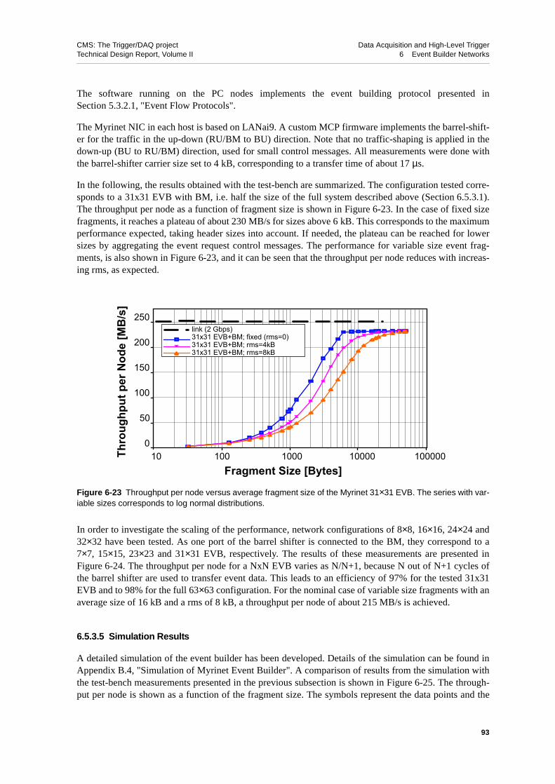
CMS: The Trigger/DAQ project Data Acquisition and High-Level TriggerTechnical Design Report, Volume II 6 Event Builder Networks
The software running on the PC nodes implements the event building protocol presented inSection 5.3.2.1, "Event Flow Protocols".
The Myrinet NIC in each host is based on LANai9. A custom MCP firmware implements the barrel-shift-er for the traffic in the up-down (RU/BM to BU) direction. Note that no traffic-shaping is applied in thedown-up (BU to RU/BM) direction, used for small control messages. All measurements were done withthe barrel-shifter carrier size set to 4 kB, corresponding to a transfer time of about 17 µs.
In the following, the results obtained with the test-bench are summarized. The configuration tested corre-sponds to a 31x31 EVB with BM, i.e. half the size of the full system described above (Section 6.5.3.1).The throughput per node as a function of fragment size is shown in Figure 6-23. In the case of fixed sizefragments, it reaches a plateau of about 230 MB/s for sizes above 6 kB. This corresponds to the maximumperformance expected, taking header sizes into account. If needed, the plateau can be reached for lowersizes by aggregating the event request control messages. The performance for variable size event frag-ments, is also shown in Figure 6-23, and it can be seen that the throughput per node reduces with increas-ing rms, as expected.
In order to investigate the scaling of the performance, network configurations of 8×8, 16×16, 24×24 and32×32 have been tested. As one port of the barrel shifter is connected to the BM, they correspond to a7×7, 15×15, 23×23 and 31×31 EVB, respectively. The results of these measurements are presented inFigure 6-24. The throughput per node for a NxN EVB varies as N/N+1, because N out of N+1 cycles ofthe barrel shifter are used to transfer event data. This leads to an efficiency of 97% for the tested 31x31EVB and to 98% for the full 63×63 configuration. For the nominal case of variable size fragments with anaverage size of 16 kB and a rms of 8 kB, a throughput per node of about 215 MB/s is achieved.
6.5.3.5 Simulation Results
A detailed simulation of the event builder has been developed. Details of the simulation can be found inAppendix B.4, "Simulation of Myrinet Event Builder". A comparison of results from the simulation withthe test-bench measurements presented in the previous subsection is shown in Figure 6-25. The through-put per node is shown as a function of the fragment size. The symbols represent the data points and the
Figure 6-23 Throughput per node versus average fragment size of the Myrinet 31×31 EVB. The series with var-iable sizes corresponds to log normal distributions.
Thro
ughp
ut p
er N
ode
[MB
/s]
Fragment Size [Bytes]
link (2 Gbps)31x31 EVB+BM; fixed (rms=0)31x31 EVB+BM; rms=4kB31x31 EVB+BM; rms=8kB
50
100
150
200
250
100
100 1000 10000 100000
93

CMS: The Trigger/DAQ project Data Acquisition and High-Level TriggerTechnical Design Report, Volume II 6 Event Builder Networks
two bands are obtained by simulation. The bands differ in the assumptions made for the performance ofthe NIC card (see Appendix B.4 for details). The points are enclosed by the two bands showing a goodagreement between the test-bench data and the simulation.
Starting from the accurate description of the current LANai9 hardware, a prediction is made for the Myri-net LANai10 hardware. The result for a 64×64 network configuration based on a one-rail network withLANai10 hardware including a BM is shown in Figure 6-26. At the working point of 16 kB fragmentsize, a throughput of 236 MB/s is expected for fixed sizes and is only slightly reduced to 231 MB/s forvariable sizes with an rms of 6 kB. This provides a comfortable safety margin for the required throughputof 200 MB/s for a trigger rate of 12.5 kHz per RU Builder.
Figure 6-24 Throughput per node versus N×N for Myrinet EVB.
Figure 6-25 Throughput per node as a function of the fragment size for a 31×31 EVB with BM and LANai9hardware. The bands represent the simulation result for two different NIC performance assumptions. The sym-bols show the data points measured with the test-bench.
Thro
ughp
ut p
er N
ode
[MB
/s]
0
50
100
150
200
250
0 5 10 15 20 25 30
N for NxN EVB
link BW (2Gbps)16 kB fixedaverage=16kB, rms=8kB
Thro
ughp
ut p
er n
ode
[MB
/s]
0
50
100
150
200
250
300
10 100 1000 10000 100000
Fragment size [Bytes]
DataSimulation 1Simulation 2
94

CMS: The Trigger/DAQ project Data Acquisition and High-Level TriggerTechnical Design Report, Volume II 6 Event Builder Networks
6.6 Readout Control Network
The Readout Control Network (RCN) is a component of the RU Builder. It is used to distribute readoutinformation that is common to all the RUs in the RU Builder. This information includes the association ofEvent-ID to the Level-1 event number (Section 4.3, "RU Builder").
6.6.1 Overview of RCN Requirements
The RCN is the logical network used by the Event Manager to distribute control information to all RUs ina single RU Builder (partition). The main requirements are therefore:
• The RCN must handle 64 nodes (1 RM and 63 RUs).
• The distribution of the RCN messages must be reliable.
• Network support for broadcast/multicast may be used to reduce the number of messages sent bythe RM because the data content of the RCN message is identical for all RUs.
• The maximum event rate in a RU Builder is 12.5 kHz, which correspond to an average time be-tween events of 80 µs. It is difficult to broadcast a message reliably below 1 ms with current com-mercial network technologies on a PC. However, the broadcast rate can be reduced by packingseveral messages in each broadcast. Packing of several tens of messages per broadcast would re-duce the rate sufficiently.
• The minimum information to be sent for each event is the “Event_ID/event number” pair, whichrequires 8 bytes. It may be desirable to send more information such as the Bunch crossing number.The design is not yet finalised at this level.
• Assuming that 12 bytes per event are distributed per broadcast, then the effective bandwidth need-ed (discarding overheads) would be 12 B × 12.5 kHz = ~1.2 Mbps which corresponds to 0.12% ofthe bandwidth available on Gigabit Ethernet. Peer-to-peer communication between the EVM andthe RUs would increase the RCN traffic by a factor 63, requiring an effective bandwidth of63 × 1.2 Mbps or 8% of the Gigabit Ethernet bandwidth at the EVM port.
Figure 6-26 Simulated throughput as a function of the fragment size for a 63×63 EVB with BM and LANai10hardware in a one-rail network.
Thro
ughp
ut p
er n
ode
[MB
/s]
Average fragment size [Bytes]
0
50
100
150
200
250
10 100 1000 10000 100000
95

CMS: The Trigger/DAQ project Data Acquisition and High-Level TriggerTechnical Design Report, Volume II 6 Event Builder Networks
• The latency requirement on delivery of the Event_ID is relaxed because the Event-IDs are assignedto super-fragments only after these have been buffered in the RU memory (see Section 4.3.7, "RUBuilder Data Flow"). With a RU buffer depth of O(512 MB), corresponding to 32000 super-frag-ments of 16 kB, it is possible to accept latencies of several thousand triggers. It is therefore not aproblem to pack several tens of RCN messages per broadcast.
• The network must be consistent with partitioning of the RU Builder. This means that it must bepossible to send the RCN messages to only a subset of the RUs either in multicast or peer-to-peermode.
6.6.2 Implementation
RCN can be implemented as a Gigabit Ethernet physical network distinct from the Builder network or itcan be integrated with the BCN and BDN in one builder network as described in Section 5.4.2, "EventManager Networks". This implementation choice has not yet been made.
If RCN is implemented on a distinct Gigabit Ethernet network, it is possible to use multicast over UDPfor distribution of the RCN messages to the RUs. A reliable broadcast protocol has been developed to sat-isfy the requirement of reliable delivery of RCN messages.
6.6.3 Reliable Broadcast Protocol for the RCN
The distribution of the RCN control information must be totally reliable, which means no loss of informa-tion and guaranteed latency. There are many broadcast/multicast protocols proposed or implemented.Most of them aim to serve multimedia (audio/visual) data streams and are not totally reliable. Some ofthem guarantee total reliability, but are not fast enough, because the main applications of these are filetransfer and data mirroring.
The proposed RCN Protocol (RCNP), copes with both total reliability and low (O(ms)) latency. It is acombination of popular techniques and utilizes knowledge of the network topology and usage of the RCNto reduce the latency.
Key features of the RCNP are:
• It is NACK-based
• It includes packet loss detection on the receiver side
• It has redundancy to reduce packet repairs
• It utilizes acknowledgments (ACKs) from a few clients as a pacemaker.
ACK-based mechanisms, in which each receiver sends back an ACK packet for every data packet, are notapplicable given the message rate and latency in the RU Builders. A flat network would be flooded withACK packets while a tree-based ACK mechanism introduces a significant latency. This problem is moresevere with slower systems like Fast Ethernet. In a NACK(Negative ACK)-based mechanism, a receiversends back a repair request only when it detects packet losses or unrecoverable corruptions.
Data corruptions inside a packet are detected utilizing CRC (cyclic redundancy check) words included ineach packet. Packet losses are detected as jumps between the sequential numbers of adjacent packets. Thesequential number may be the L1 trigger number in our case. With these mechanisms the data can alreadybe transmitted reliably. However, the process of repairing packets is expensive in terms of latency. There-
96

CMS: The Trigger/DAQ project Data Acquisition and High-Level TriggerTechnical Design Report, Volume II 6 Event Builder Networks
fore a Forward-Error Correction (FEC) technique is introduced to keep the packet retransmissions as rareas possible. In this scheme, the RM sends redundant data and any receiver can reconstruct the originaldata allowing for packet losses up to the redundancy limit. A simple example is to add one extra packet,that is the XOR of original packets, for every three data packets (3+1 FEC). In that case the receiver miss-es the data only when there are two or more packets lost from these four packets. Any fraction of redun-dancy is possible regarding the network reliability.
The last point is congestion control. There is no means to detect buffer overflow on the receiver side, be-cause hardware flow control is not possible (or not practical) in broadcasts. Keeping the transfer rate be-low a level acceptable for the RUs is necessary to avoid buffer overflows and resulting NACK floods. Apossible method is that the EVM waits for a ACK packet from only one or a few RUs and sends out thenext packet after receiving it. Using this method the EVM applies an optimized delay between sends.
The RCNP, described above, is illustrated in Figure 6-27. In case of no packet loss or corruption (leftside), trigger information is sent as a sequence of packets, which consists of three original data and a re-dundancy packet for 3+1 FEC. One or several preconfigured RUs send back an ACK packet. Then, theEVM starts sending the next sequence. If packet losses occur (right side), the incomplete sequence is de-tected when a packet for the next (or later) sequence is received by a RU. The RU sends back a NACKpacket to the EVM and the EVM sends the lost packet sequence again as a broadcast.
6.6.4 RCN Prototype and Simulation
Prototyping and simulation studies of the RCN have been performed in conjunction with the EVM proto-typing and simulation described in Section 5.4.5, "Prototypes for the Event Manager". The studies havenot yet reached a final conclusion, but they have reached a level, where there is no doubt that the RCNcan be implemented using one or more of the possible implementations under study.
Figure 6-27 RCNP - a protocol for the RCN.
Sequence n(packet 1)(packet 2)(packet 3)(packet X)ACK
Sequence n(packet 1)(packet 2)(packet 3)(packet X)ACK
Sequence n+1(packet 1)(packet 2)(packet 3)(packet X)ACK
EVM RU
EVM RU
Sequence n(packet 1)(packet 2)(packet 3)(packet X)
Sequence n+1(packet 1)NACK
Lost
(packet 2)(packet 3)(packet X)ACK
97
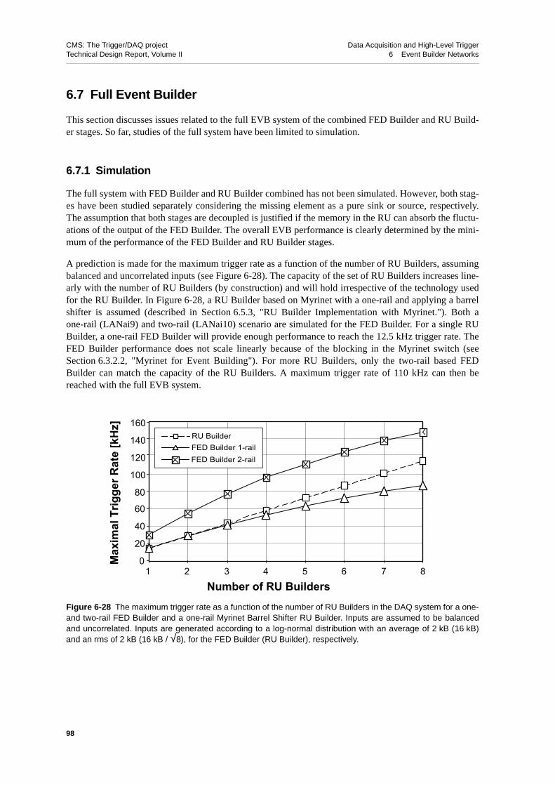
CMS: The Trigger/DAQ project Data Acquisition and High-Level TriggerTechnical Design Report, Volume II 6 Event Builder Networks
6.7 Full Event Builder
This section discusses issues related to the full EVB system of the combined FED Builder and RU Build-er stages. So far, studies of the full system have been limited to simulation.
6.7.1 Simulation
The full system with FED Builder and RU Builder combined has not been simulated. However, both stag-es have been studied separately considering the missing element as a pure sink or source, respectively.The assumption that both stages are decoupled is justified if the memory in the RU can absorb the fluctu-ations of the output of the FED Builder. The overall EVB performance is clearly determined by the mini-mum of the performance of the FED Builder and RU Builder stages.
A prediction is made for the maximum trigger rate as a function of the number of RU Builders, assumingbalanced and uncorrelated inputs (see Figure 6-28). The capacity of the set of RU Builders increases line-arly with the number of RU Builders (by construction) and will hold irrespective of the technology usedfor the RU Builder. In Figure 6-28, a RU Builder based on Myrinet with a one-rail and applying a barrelshifter is assumed (described in Section 6.5.3, "RU Builder Implementation with Myrinet."). Both aone-rail (LANai9) and two-rail (LANai10) scenario are simulated for the FED Builder. For a single RUBuilder, a one-rail FED Builder will provide enough performance to reach the 12.5 kHz trigger rate. TheFED Builder performance does not scale linearly because of the blocking in the Myrinet switch (seeSection 6.3.2.2, "Myrinet for Event Building"). For more RU Builders, only the two-rail based FEDBuilder can match the capacity of the RU Builders. A maximum trigger rate of 110 kHz can then bereached with the full EVB system.
Figure 6-28 The maximum trigger rate as a function of the number of RU Builders in the DAQ system for a one-and two-rail FED Builder and a one-rail Myrinet Barrel Shifter RU Builder. Inputs are assumed to be balancedand uncorrelated. Inputs are generated according to a log-normal distribution with an average of 2 kB (16 kB)and an rms of 2 kB (16 kB / √8), for the FED Builder (RU Builder), respectively.
0
20
40
60
80
100
120
140
160
1 2 3 4 5 6 7 8Number of RU Builders
Max
imal
Trig
ger R
ate
[kH
z]
RU BuilderFED Builder 1-railFED Builder 2-rail
98

CMS: The Trigger/DAQ project Data Acquisition and High-Level TriggerTechnical Design Report, Volume II 6 Event Builder Networks
6.8 Summary and Outlook
This chapter described the design and possible implementations of the Event Builder networks. Atwo-stage EVB design with 64 8×8 switches in the FED Builder stage and 8 64×64 switches in the RUBuilder stage has been considered. A major advantage of this architecture compared to a single 512×512monolithic switching network is that the RU and BU nodes need to operate at a rate of only 12.5 kHz withaverage fragment sizes of 16 kB, rather than at 100 kHz with average fragment sizes of 2 kB.
A possible configuration of the FED Builder stage connecting the total of ~630 FEDs in the CMS readouthas been outlined. The proposed assignment of FEDs to FED Builders provides reasonable balanced in-puts to the second stage of the Event Builder.
The two-stage Event Builder design, consisting of FED Builder and RU Builder, imposes very differentrequirements on the two builder networks. Two networking technologies, Ethernet and Myrinet, havebeen considered for each of the two stages.
6.8.1 FED Builder
The 8×8 FED Builder is required to handle a 100 kHz rate of fragments with sizes ranging from a fewhundred bytes to a few kilobytes and combine them into super-fragments.
The results from the FED Builder prototype combined with simulation studies show that the FED Buildercan be implemented with a two-rail Myrinet configuration and LANai10 based NICs. It can be designedto deliver super-fragments in sequential order to the RU at the required 12.5 kHz rate with a low overheadon the RU.
The difficulty of meeting the requirements with Ethernet equipment available in 2002 was judged toohigh to warrant a prototyping effort.
6.8.2 RU Builder
The requirement of the 64×64 RU Builder with a 12.5 kHz rate of 16 kB fragments can be met with Myri-net and most likely also with Ethernet technology. The equipment available for prototyping allowed test-ing of RU Builders of half the required size.
6.8.2.1 Myrinet
The measurements on the half-sized RU Builder (32×32) proved that Myrinet can perform event buildingin barrel shifter mode at near 100% utilization of the network bandwidth. The simulation model describesthe equipment accurately and shows good agreement between measured and simulated results. Simulationestimates of the performance of a full RU Builder show that a one-rail Myrinet configuration will meetthe requirements of a full RU Builder.
6.8.2.2 Gigabit Ethernet with Layer-2 Frames
Tests have been done with a one-rail 32×32 and a two-rail 16×16 Gigabit Ethernet RU Builder. Theseconfigurations corresponded to half and one quarter of the full size, respectively. Both measurementsshow that with a lightweight protocol using Layer-2 frames it is possible to operate in event building
99
CMS: The Trigger/DAQ project Data Acquisition and High-Level TriggerTechnical Design Report, Volume II 6 Event Builder Networks
mode near 100% utilization of the network bandwidth. The performance is critically dependant on theamount of internal buffer memory of the switch to ensure a low packet loss probability. A simple simula-tion model, which does not yet include the recovery from packet loss, shows good agreement betweenmeasurements and predicted throughput. It is plausible, but not proven, that a two-rail Gigabit EthernetEvent Builder with Layer-2 frames will meet the requirement of a full RU Builder. This solution wouldrely on standard hardware, but requires non-standard software and application level traffic-shaping anderror recovery. Only the TCP/IP based solution described below would bring the full advantage of stand-ard Ethernet hardware and software to the RU Builder.
6.8.2.3 Gigabit Ethernet with TCP/IP
The equipment available for prototyping could operate TCP/IP only at 70% of the available bandwidth inpoint-to-point communication and at 60% of the available bandwidth in event building with a (32×32)one-rail and a half-sized RU Builder. The result is encouraging, but inconclusive, because the PCs andtheir NICs are only loading the switch at 60%. New models of PCs and NICs have been measured to op-erate at near 100% of available bandwidth over a two-rail point-to-point TCP/IP communication. Howev-er, these systems were not available in quantities that allowed RU Builder testing.
The measurement made so far shows that TCP/IP over Gigabit Ethernet might meet the RU Builderthroughput requirements when operated on PCs with more than 2 GHz Pentium-IV Xeon processors andappropriate NICs. It is still an open question whether TCP/IP based event building will work when theswitch is operated closer to full capacity. It is difficult to simulate the TCP/IP traffic accurately, becauseof the complexity and because of missing information on the inner operation of the switches, the NIC andsystem level TCP/IP software. A complete proof of the TCP/IP option can probably only be obtainedthrough prototyping with a full-scale one-rail RU Builder using equipment that can drive TCP/IP at fullrate in point-to-point mode.
6.8.3 Readout Control Network
The RCN can be implemented as a Gigabit Ethernet physical network distinct from the Builder networkor it can be integrated with the Builder network. Although the final implementation choice has not yetbeen made, the problem is reduced to finding the optimal out of several possible solutions.
6.9 Conclusion
It has been demonstrated that the EVB can be implemented with technology available in 2003. In the caseof the FED Builder the requirements can be met with Myrinet and in the case of the RU Builder they canbe met with both Myrinet and Gigabit Ethernet.
The EVB architecture is flexible enough to be implemented with other network technologies as well. Po-tential candidates for future feasibility studies include 10-Gigabit Ethernet and Infiniband [6-10]. The fi-nal choice of technology will be made based on numerous considerations including cost, ease ofoperation, maintenance and ease of upgrades.
100

CMS: The Trigger/DAQ project Data Acquisition and High-Level TriggerTechnical Design Report, Volume II 6 Event Builder Networks
6.10 References
6-1 M. Bellato et al., “The CMS Event Builder Demonstrators based on GigaEthernet Switched Network”, in Proceeding of the CHEP2000 Conference, Padova, Italy, 7-11 Feb. 1999, pp. 303-306.
6-2 G. Antchev et al., “The CMS Event Builder Demonstrator and results with Myrinet”, Comput. Phys. Commun., 140 (2001) 130.
6-3 E. Barsotti, A. Booth and M. Bowden, “Effects of Various Event Building Techniques on Data Acquisition System Architectures”, Santa Fe Computing 1990:82-101, http://fnalpubs.fnal.gov/archive/1990/conf/Conf-90-061.pdf
6-4 N.J. Boden et al., “Myrinet - A Gigabit per Second Local Area Network”, IEEE-Micro, February 1995, Vol. 15, No. 1, pp. 29-36.
6-5 VITA Standards Organization, “Myrinet-on-VME protocol specification”, ANSI/VITA 26-1998.
6-6 Myrinet products from Myricom, Inc.,Arcadia, CA, USA, see http://www.myri.com
6-7 O. Kodolova, I. Tomalin and P. Yepes, “Expected Data Rates from the Silicon Strip Tracker”, CMS Note-2002/047.
6-8 FastIron switch from Foundry Networks, see http://www.foundry.com
6-9 AceNIC from Alteon Corp., see http://www.alteon.com
6-10 Infiniband, see http://www.inifinibandta.org
101

CMS: The Trigger/DAQ project Data Acquisition and High-Level TriggerTechnical Design Report, Volume II 6 Event Builder Networks
102

CMS: The Trigger/DAQ project Data Acquisition and High-Level TriggerTechnical Design Report, Volume II 7 Readout Column
7 Readout Column
The previous chapters of Part 2 have dealt with data flow from the standpoint of event building and havediscussed the related flow control. This chapter discusses the components which provide the functionalityto read out the front-end electronics, transfer the data from the underground experimental area to the sur-face, and buffer them before the complete event can be assembled. These components are collectively re-ferred to as a Readout Column. The next section gives an overview of the structure of the ReadoutColumn. Section 7.2 summarizes the readout requirements of the various sub-detectors. A functional de-scription of the column components can be found in Sections 7.3, 7.4 and 7.5. Section 7.6 explains howthe data flow in the column is controlled via the Trigger-Throttling System (TTS). In Section 7.7 a de-scription of the prototypes and test-benches built so far, and a summary of the measurements obtainedwith them, are given. A summary section concludes the chapter.
7.1 Introduction
The Readout Column is a vertical slice of the DAQ system which consists of a Front-End Driver (FED),reading out the Front-End Systems, and feeding these data into a Front-end Readout Link (FRL). TheFRL output is carried to the surface part of the FED Builder, where it is assembled into a larger data struc-ture and stored in a Readout Unit (RU) (see Figure 7-1).
The FES and the FED, up to the interface with the DAQ, are subdetector-specific components.There areapproximately 10,000 FES modules in the CMS readout, all located in the underground area. For everyevent accepted by the Level-1 Trigger, several Front-End Systems send data to a FED. The Front-EndSystem (FES), and at least part of the FED, operate synchronously with the LHC clock. They are drivenby fast synchronous signals distributed by the Trigger Timing and Control system (TTC) [7-1]. Examplesfor these signals are the Level-1 Trigger, the 40 MHz LHC clock (BX) and reset signals to synchronizethe various Front-End Systems amongst each other. The transfer of data from the FED to the FRL is notsynchronized to the LHC clock, and, therefore, the rest of the Readout Column operates asynchronously.
In order to provide common handling of event fragments from the different subdetectors, the interface be-tween the FED and the DAQ system has been standardized in the S-LINK64 specification [7-2]. TheS-LINK64 transfers data from the FED to the Front-end Readout Link (FRL). To reduce the number ofFED Builder input ports, and to balance input fragment sizes for efficient operation of the FED Builderswitch, event fragments from up to two FEDs can be merged into a single data block in the FRL. TheFED Builder switch itself is located on the surface, at a distance of about 200 m from the FRL. A long op-tical link is used to transfer data from the underground experimental area to the surface. The FED BuilderInput (FBI) drives this link using the FED Builder communication protocol.
Event data blocks from the FRLs are organized in the RU memory to form an event super-fragment con-taining data from several FEDs. The RU is the largest data buffer in the Readout Column. This large buff-er is needed to decouple the final event building from the readout operations performed in the ReadoutColumn. From the RU, data are transferred, via the RU Builder, to the Builder Unit (BU), which assem-bles event super-fragments from many RUs to form entire events. Subsequently, these events are trans-ferred to a Filter Column (FC) where they are processed in order to obtain the High-Level Triggerdecision (HLT).
103

CMS: The Trigger/DAQ project Data Acquisition and High-Level TriggerTechnical Design Report, Volume II 7 Readout Column
7.2 Detector Readout Requirements
This section summarizes the requirements of the sub-detectors relevant for the DAQ system. For an ex-haustive description of each CMS sub-detector, the reader is referred to the corresponding Technical De-sign Reports [7-3][7-4].
7.2.1 Requirements Common to all Sub-detectors
This part describes the generic functions performed by each front-end electronics. Although their imple-mentation is specific, they all follow a common logical model described in [7-5] and illustrated inFigure 7-2.
All sub-detectors generate analog signals which are processed in several stages by the front-end electron-ics. The signal path then splits into one for the DAQ system and another for the trigger system1. Trigger
Figure 7-1 Location of the readout column in the CMS DAQ. Also shown are the main elements in the ReadoutColumn, namely the FED, the FED Builder and the Readout Unit. The FED Builder contains the data link to thesurface (D2S).
1. Not all sub-detectors send information to the Level-1 Trigger system.
RTP FECTPG
TTC
sTTSaTTSGTP
LV1 FED
FES
DCS
RU
EVMRM-BM
BU
FFNFU
BDN
DCN
DSN
RCMSCSN
DSNRCN
BCN
FRL-FB(D2S)
*700
*10000
*512
RUI
RUO
BUI
BUO
DAQ ControlTrigger &column columnData Flow Control
*64x8
*64x8
*8
*8
*8*8
AcronymsBCNBDNBMBUCSNDCSDCNDSND2SEVMFBFECFEDFESFFNFRLFSGTPLV1RTPRMRCNRCMSRUTPGTTCsTTSaTTS
Builder Control NetworkBuilder Data NetworkBuilder ManagerBuilder UnitComputing Service NetworkDetector Control SystemDetector Control NetworkDAQ Service NetworkData to SurfaceEvent ManagerFED BuilderFront-End ControllerFront-End DriverFront-End SystemFilter Farm NetworkFront-End Readout LinkFilter SubfarmGlobal Trigger ProcessorLevel-1 Trigger ProcessorRegional Trigger ProcessorReadout ManagerReadout Control NetworkRun Control and Monitor SystemReadout UnitTrigger Primitive GeneratorTiming, Trigger and Control synchronous Trigger Throttle Systemasynchronous Trigger Throttle System
104

CMS: The Trigger/DAQ project Data Acquisition and High-Level TriggerTechnical Design Report, Volume II 7 Readout Column
information is transmitted synchronously with the LHC machine clock via a dedicated link to the triggerlogic. There it is processed to obtain the Level-1 Trigger decision.
On the DAQ path, data must be buffered during the processing time of the Level-1 Trigger. Since the trig-ger system operates synchronously to the LHC machine clock, the arrival time of the trigger decision atthe Front-End System is fixed. Therefore the data buffer is implemented with a pipeline (analog or digit-al) driven by the LHC clock. The length of the pipeline is calibrated to the latency of arrival of the Lev-el-1 decision signal. On a positive trigger decision data is written into a “derandomizer” buffer which hasthe functionality of a FIFO.
For every Level-1 Trigger the contents of several derandomizer buffers are merged to form event frag-ments. In order to identify the event fragment and to allow for consistency checks in the DAQ system, theheader contains the event number and the bunch-crossing identifier. Both numbers are generated locallyin the Trigger Timing and Control receiver chip (TTCrx). The formatted event fragments are transmittedinto the Readout Column.
7.2.2 Front-end Buffer Overflow Management
Space and power constraints in the front-end electronics only allow to implement small derandomizerbuffers. Since the Level-1 Trigger is distributed statistically in time, and for each sub-detector there is aminimal derandomizer specific readout time (called service time), the buffer can in principle overflow.
Figure 7-2 CMS front-end common logical model.
CLOCK 40.08 MHz
L-1 TRIGGER
EVENT COUNTER
TIMING, TRIGGER AND CONTROL DISTRIBUTION SYSTEM
PIPELINE (ANALOGUE/DIGITAL)
DERANDOMIZER
READOUT WINDOW
(PROCESSING ELEMENT)
(PROCESSING ELEMENT)EC RESET
BUNCH COUNTERBC RESET
TRIGGERPRIMITIVE
GENERATOR
(ADC, PROCESSING ELEMENT)
FE IDENTIFIER
FORMATTING
TEST SIGNALS
INITIALIZATION
PARAMETERS
FAST CONTROLS
TIME TAGEVENT TAG
READOUT LINK INTERFACE
BACK PRESSURE
MULTIPLEXER (SPARSE READOUT)
Buffer status, Error reports
Detector channel
FrontEnd System
Data acquisition
Frontend model
Trigger link
TTSTrigger Throttle System
TTCTiming, Trigger and Control
105

CMS: The Trigger/DAQ project Data Acquisition and High-Level TriggerTechnical Design Report, Volume II 7 Readout Column
Table 7-1 lists the service time and buffer sizes for each of the various sub-detectors. In case of an over-flow, most sub-detectors drop the event data and continue to transmit empty events until the buffers areready to receive new event fragments. This allows to retain synchronization with the DAQ system andhence avoids lengthy recovery procedures that would deteriorate the DAQ efficiency.
In order to minimize the probability of a buffer overflow, rules which limit the number of triggers in afixed time interval are applied in the Global Trigger Processor. Table 7-1 summarizes the result of simula-tions (if available) for the various sub-detectors, assuming different trigger rules and 100 kHz trigger rate.As can be seen, buffer overflows can not be avoided completely by introducing trigger rules. Therefore,where possible, the Global Trigger Logic (GTL) emulates the state of the front-end buffers in order tosuppress triggers which would cause a buffer overflow.
Finally, the Front-End Systems assert fast signals to throttle the trigger via the synchronous Trig-ger-Throttling System (sTTS) described in Section 7.6.
Table 7-1 Front-end and overflow management.
DetectorBuffer size (events)
Service time (us)
Overflow probabilityw/o Trigger rule
Front-end Emulation
Derandomizer Warning signals
Trigger rules
Pixel 16 N/A < 2.5%a
a. on-going simulation work.
not possible (all the Front-ends are independent)
status bit in the data stream (3 levels of warn-ing)
empty orbit every second and at least 2 empty BX between consecutive triggers
Tracker 10 7 3.10-4 b
b. extracted from [7-6].
Hardware emula-tor based on APV core [7-7]
no at least 2 empty BX between consecutive triggers
Preshower 10 5.4 2.10-5 b simple state machine
yes no more than N+7 triggers during N x service time
ECAL 25 7.1 very low easy emulation if needed
no (considered to be too slow)
none
HCAL 44 4 very low not needed notneeded
no more than 22 trig-gers per orbit
Muons CSC ~85 0.3/3/26 0.3 events/24 hours
no yes at least 2 empty BX between consecutive triggers
Muons RPC 64 8 very low not possible (occupancy dependent)
yes none
Muons DT 16 2 very low not possible (occupancy dependent)
yes none
106

CMS: The Trigger/DAQ project Data Acquisition and High-Level TriggerTechnical Design Report, Volume II 7 Readout Column
7.2.3 Sub-detector Readout Parameters
In this paragraph the readout parameters of the various sub-detectors are summarized. A comprehensivedescription of the detector geometry, the readout chain and the data format are available from [7-8] andfrom Chapter 14, "Detector Simulation and Reconstruction". Table 7-2 lists the number of sub-detector
specific data sources. The fifth column shows the number of data sources for the DAQ system. The ex-pected event sizes of some of these are so small that two data sources can be merged to single event frag-ments in the Front-end Readout Link (see Section 7.4). This reduces the total number of data sources tothe Front-End Driver Builder to 468.
Expected event fragment sizes, total event size and its rms-estimate of the various sub-detectors for pp(high luminosity run) are sumamrized in Table 7-3. The average expected event size is approximately680 kB. To account for remaining uncertainties on these average estimates, the average event size isrounded up, for contingency, to 1 MB throughout the rest of this TDR. The DAQ system is therefore de-signed to handle average event sizes up to 1 MB.
The event sizes for Pb-Pb operation of LHC are dominated by the event sizes of the tracker. The design ofthe DAQ system does not impose any limit on the size of the events as long as the average data through-put per data source does not exceed 200 MB/s. In Section 14.3.2.1.3, "Tracker Data Format and DataRates" it is shown, that at the estimated interaction rate of 8 kHz, the increased event size of the Tracker iscompatible with this data throughput.
Table 7-2 Detector readout chain comparative overview.
DetectorNumber ofchannels
Number of FE chips
Number of detector data links
Number of data sources
Number ofDAQ links
Pixel ~44M 15840 1504 38 38
Tracker ~9.3M ~72k ~36k 440 272 (merged)
Preshower 144384 4512 1128 47 47
ECAL 82728 ~17k ~9k 54 (DCC) 54
HCAL 9072 9072 3072 32 (DCC) 32
Muons CSC ~500k ~76k 540 8 (DCC) 8
Muons RPC 192k ~8.6k 636(732)a
a. The figure in parentheses is the number of links with station 5 extension.
6 (DCC) 6
Muons DT 195k 48820 60 5 (DCC) 5
Global trigger N/A N/A N/A 4 4
DT track finder N/A N/A N/A 1 1
CSC track finder N/A N/A N/A 1 1
Total ~54.5M -- -- 636 468
107

CMS: The Trigger/DAQ project Data Acquisition and High-Level TriggerTechnical Design Report, Volume II 7 Readout Column
7.3 The Common Interface between the FEDs and the DAQ System
A basic design principle for the CMS DAQ system is the handling of event fragments from all CMSsub-detectors in the same way [7-8], so that the event-building process can be implemented with a uni-form set of hardware and software components, independent of the data source. For this reason, a stand-ard interface from the FED to the DAQ system has been designed. The interface specifies a commonhardware platform and a data format which is a header and a trailer with information relevant to the eventbuilding process. The payload of the event fragments is only inspected in the filter farm, i.e. it is not con-sidered during event building. As a result of this common interface, there is no sub-detector specific hard-ware after the FED in the readout chain.
7.3.1 Front-End Driver Overview
The main function of the Front-End Driver (FED) is to read out a number of FES modules, store the datain an intermediate buffer, and provide them to the DAQ via a common interface. The FED consists of twofunctional blocks as shown in Figure 7-3. The first block contains all functionality specific to each indi-vidual sub-detector while the second block contains the interface to the DAQ.
The Readout Column is designed for an average event fragment size of 2 kB which at the maximum eventrate of 100 kHz corresponds to a sustained data throughput of 200 MB/s. For sub-detectors which deliversignificantly smaller event fragments, a Data Concentrator Card (DCC) is developed in order to mergeseveral small fragments into one fragment of approximately 2 kB. In these cases it is the DCC that inter-faces to the DAQ system.
Table 7-3 Event sizes and variations for pp (high luminosity).
DetectorEvent size per DAQ link pp (kB)
Total event size pp (kB)
rms of total event size pp
Pixel 1.8 - 2.0 72 ~30%
Tracker 0.4 - 1.5 a 300 ~30%
Preshower 2.3 110 tbdb
ECAL 2 ~100 ~20%
HCAL 2 64 ~80%
Muons CSC 1.5 12 ~80%
Muons RPC 0.3 1.5 ~30%
Muons DT 1.6 8 tbd
Global trigger 2 8 none
DT track finder 2 2 none
CSC track finder 1 1 tbd
Total -- 678.5
a. see [7-9] for event size distribution.
b. to be defined - no information available at the time of writing.
108

CMS: The Trigger/DAQ project Data Acquisition and High-Level TriggerTechnical Design Report, Volume II 7 Readout Column
During operation, the FED must provide the Trigger Control System (TCS) with status information (seeSection 7.6). In case of an imminent buffer overflow, the FED uses the TCS to throttle or inhibit furtherLevel-1 Triggers. Once data in the buffers have been successfully transmitted to the DAQ, the TCS sys-tem is notified and triggers resume at full rate. The system is also used to indicate error conditions in theFED. In these cases the Control and Monitor system (see Chapter 12, "Run Control and Monitor System")must take appropriate actions.
For various purposes like monitoring, local DAQ operation, calibration or debugging, each FED imple-ments a local DAQ interface, allowing the readout of event fragments via a local bus interface (VME orPCI). The hardware implementation of this is FED specific. The software environment, however, is pro-vided by the XDAQ system (see Chapter 10, "Online Software").
7.3.2 Hardware of the FED Interface to the DAQ
The interface to the DAQ is an S-LINK64 interface [7-2]. The S-LINK64 protocol is based on S-LINKwhich has been extended to match the CMS needs for higher bandwidth (64 bits data width and 100 MHzmaximum input rate, instead of 32 bits data width and 40 MHz maximum input rate for S-LINK). BothS-LINK and S-LINK64 only specify a set of connectors for sending and receiving data, along with me-chanical constraints for the sender and the receiver cards. The physical link between them is not specifiedbeyond these constraints. In addition, both interfaces specify the protocols for writing into the sender cardand reading from the receiver card. Both protocols resemble standard protocols that read from and writeto a synchronous FIFO. A built-in test mode allows to verify the correct functioning of the link.
Figure 7-3 Functional block diagram of the Front-End Driver (FED).
Specific
Detector
Electronic
S-LI
NK6
4 po
rtD
ata
port
Con
trol p
ort
Stat
us p
ort
LinkFPGA
FED/DCCD
etec
tor l
inks
Storagearea
VME HostInterface
109

CMS: The Trigger/DAQ project Data Acquisition and High-Level TriggerTechnical Design Report, Volume II 7 Readout Column
7.3.3 FED Data Format
The FED encapsulates the data received from the FES in a common data structure by adding a header anda trailer that mark the beginning and the end of an event fragment. Their content consists of event infor-mation partly used in the event building process.
In Table 7-4 the various data fields in the header and trailer, also shown in Figure 7-4, are described.Since the number of reserved bits in the format is small, the number of header words can be increased dy-namically (see “H”- field). This ensures flexibility for future changes.
7.4 Front-end Readout Link
The event fragments of the FED are transferred via the S-LINK64 interface to the FED Builder. The inter-face between the S-LINK64 receiver card and the FED Builder is called the Front-end Readout Link(FRL) and provides the FED Builder with event fragments. The protocol used by this interface has beendeveloped for a FED Builder built on Myrinet technology and is discussed in detail in Section 7.7.4.
Although some sub-detectors develop Data Concentrator Cards in order to provide the DAQ system withevent fragments of 2 kB on average, a significant number of FEDs are expected to provide event frag-ments with less than 1 kB average size (see Section 7.2). In order to reduce the number of inputs to theFED Builders and to better exploit the available bandwidth in the event builder, the FRL is able to mergedata from two FEDs into a single event fragment. The merging is done by concatenating the two incom-ing fragments for each event in the FRL memory to form a single data block.
The current design of the FRL is a Compact-PCI card with three interfaces:
• Input interface which can host up to 2 S-LINK64 receiver cards.
• Output interfaces to the FED Builder Input (FBI) - currently implemented as a PCI bus since theFBI is a PCI-Myrinet Network Interface Card (NIC). This NIC, along with the optical fibre, imple-ments the data link to the counting room on the surface.
• Configuration and control interface, implemented as a Compact-PCI interface.
Figure 7-4 The format of the header and trailer 64-bit words in the common data encapsulation. The meaningof the various fields is described in Table 7-4. The K or D field denote a 65th bit transmitted over the SLINK64,which allows to unambiguously differentiate between the payload on one side and the header or trailer words onthe other side. This bit is necessary in the S-LINK64 receiver to identify the end of an event fragment.
60 5963 032 31
60 5963 032 31 24 23 20 19 4 3
4 3
Evt _stat(8) xx $$
BOE_1K LV1_id(24) BX_id(12)
CRC (16)
D Sub-detector payload
K
D Sub-detector payload
Evt_ty
EOE Evt _lgth (24)xxxx
Source_id(10+2) FOV
xxxx
$$Hx
BOE_2K $$
110
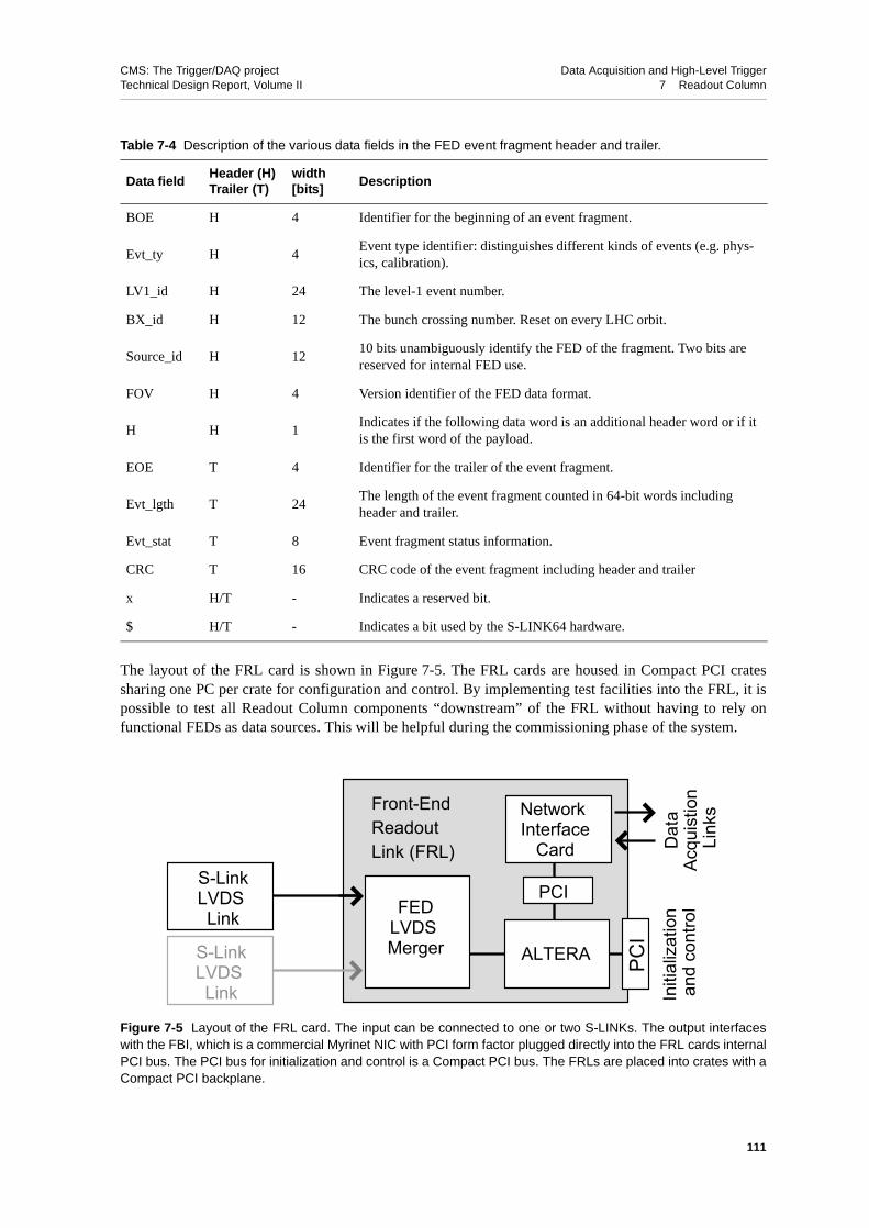
CMS: The Trigger/DAQ project Data Acquisition and High-Level TriggerTechnical Design Report, Volume II 7 Readout Column
The layout of the FRL card is shown in Figure 7-5. The FRL cards are housed in Compact PCI cratessharing one PC per crate for configuration and control. By implementing test facilities into the FRL, it ispossible to test all Readout Column components “downstream” of the FRL without having to rely onfunctional FEDs as data sources. This will be helpful during the commissioning phase of the system.
Table 7-4 Description of the various data fields in the FED event fragment header and trailer.
Data fieldHeader (H)Trailer (T)
width[bits]
Description
BOE H 4 Identifier for the beginning of an event fragment.
Evt_ty H 4Event type identifier: distinguishes different kinds of events (e.g. phys-ics, calibration).
LV1_id H 24 The level-1 event number.
BX_id H 12 The bunch crossing number. Reset on every LHC orbit.
Source_id H 1210 bits unambiguously identify the FED of the fragment. Two bits are reserved for internal FED use.
FOV H 4 Version identifier of the FED data format.
H H 1Indicates if the following data word is an additional header word or if it is the first word of the payload.
EOE T 4 Identifier for the trailer of the event fragment.
Evt_lgth T 24The length of the event fragment counted in 64-bit words including header and trailer.
Evt_stat T 8 Event fragment status information.
CRC T 16 CRC code of the event fragment including header and trailer
x H/T - Indicates a reserved bit.
$ H/T - Indicates a bit used by the S-LINK64 hardware.
Figure 7-5 Layout of the FRL card. The input can be connected to one or two S-LINKs. The output interfaceswith the FBI, which is a commercial Myrinet NIC with PCI form factor plugged directly into the FRL cards internalPCI bus. The PCI bus for initialization and control is a Compact PCI bus. The FRLs are placed into crates with aCompact PCI backplane.
Network Interface
Card
ALTERA
Front-End Readout Link (FRL) D
ata
Acqu
istio
n Li
nks
Initi
aliz
atio
n a
nd c
ontro
l
PCI
PCI
S-LinkLVDS Link
S-LinkLVDS Link FED
LVDS Merger
111

CMS: The Trigger/DAQ project Data Acquisition and High-Level TriggerTechnical Design Report, Volume II 7 Readout Column
In Figure 7-6 the FRL is shown in the context of the S-LINK64 and the FED Builder.
7.5 Readout Unit (RU)
Data fragments are assembled in the FED Builder into super-fragments with an average size of 16 kB perevent (see Section 4.2, "FED Builder"). For simplicity, super-fragments will be referred to as “fragments”in the rest of this chapter. The Readout Unit (RU) buffers these fragments and sends them, via the Read-out Unit Builder switch, to the Builder Unit (BU) which assembles the fragments into full events.
The Readout Unit is the main buffer in the data stream and is used to decouple the event building processin the RU Builder from the corresponding process in the FED Builder. This memory is necessary to ab-sorb the latency of event building and fluctuations of available resources in the Builder Units. The memo-
Figure 7-6 Elements in a FED Builder. The FED uses SLINK64 to communicate with an FRL. An FRL canaccept data from up to two FEDs. It hosts a Network Interface Card which connects it to the FED Builder switch.On the other side of the switch is the Readout Unit Input (RUI) which can accept data from all the FRLs con-nected to the FED Builder switch.
FED
FRL
FB
RUI
RUI-PCI (Myrinet LANai10)
PCI 5 Gbs/s Link (Myrinet LANai10)
LVDS-FED mergerUp to two FEDs per FRL
LVDS FED-FRL cable(s)
FED S-Link64 LVDS adapter
Two 2.5 Gb/s links per FRL
Detector Front-End Driver FED
Fro
nt-
En
d R
ead
ou
t L
ink
FED Builder: dual MxN switch
112

CMS: The Trigger/DAQ project Data Acquisition and High-Level TriggerTechnical Design Report, Volume II 7 Readout Column
ry will be large enough to buffer the data stream for seconds (this corresponds to several hundreds ofMB).
A block diagram of the RU is shown in Figure 7-7. The RU logically consists of an input unit, the Read-out Unit Input (RUI), an output unit, the RU Output (RUO) and a supervising unit, the RU Supervisor(RUS), which controls the RU functions. In addition the RU interfaces to the Event Manager via the Rea-dout Control Network (RCN), and to the Builder Unit via the Builder Unit Control Network (BCN). BothRCN and BCN are logical networks which are used by the event building protocol. If the RU detects adata inconsistency or an internal error which prevents it to continue to function normally, it reports this er-ror via the aTTS system.
The event fragments stored in the Readout Unit are requested by the BUs on a random-access basis sincethe Builder Units concurrently process many different events.
7.5.1 RU Implementation
The functionality of the RU can be implemented in two different ways: a custom design based on FPGAsor a fully programmable commercial component like a high-end Personal Computer (PC). Both optionshave been evaluated.
A custom board based on FPGAs with interfaces for data input and output has been built. The prototype isdescribed in detail in Appendix D, "Hardware Implementation of the Readout Unit".
With the availability of cost-effective personal computers that can meet the data throughput requirementof the RU, the ongoing development efforts focus on a software design for the RU. This approach ensuresflexibility for changes in the event building protocols, the hardware setup and the networking equipment.These changes would be more difficult to implement in a design that is based on FPGAs. The architectureof a PC allows the transfer of data from external interfaces to main memory and from there to other devic-es via system buses. Depending on the capabilities of these devices, the I/O operation can be driven by di-rect memory access (DMA) engines to avoid tying up the CPU. It can be initiated either by the CPU or byan intelligent device designed specifically to handle I/O. For this particular application the abilities of theRUI or the RUO to initiate the DMA of fragments into and out of the RU memory are exploited.
The main task of the RU is to intermediately store large amounts of data. The CPU provides the input de-vice with the available addresses in the computer’s main memory that serves as intermediate buffer forfragments. This dialogue is performed asynchronously through the use of two message-queues betweenthe CPU and the device. Event data are organized in main memory as chains of fixed sized blocks. Each
Figure 7-7 The Readout Unit and all its interfaces to other DAQ components.
sTTSaTTS
RU
BDN
DSNRCN
BCN
RUI
RUO
AchronymsBCNBDND2SFBFRLRCNRURUIRUORUSaTTS
Builder Control NetworkBuilder Data NetworkData to SurfaceFED BuilderFront-End Readout LinkReadout Control NetworkReadout UnitReadout Unit InputReadout Unit OutputReadout Unit Supervisorasynchronous Trigger Throttle System
RU
S
FRL-FB(D2S)
113

CMS: The Trigger/DAQ project Data Acquisition and High-Level TriggerTechnical Design Report, Volume II 7 Readout Column
stored chain is tagged with an identifier provided by the EVM (see Section 4.3.2). A catalogue of eventsis created which can be accessed randomly for transmission. The described mechanism avoids CPU-in-tensive data-copy operations (only two DMA operations per data block are involved). All means to per-form these tasks efficiently are provided by the buffer-loaning scheme of the online-softwareinfrastructure described in Section 11.2.3, "Memory Management".
7.6 Flow Control and Front-end Synchronization
The DAQ system has been designed to match the needs resulting from the LHC parameters, the propertiesof the expected physics events and the architecture of the detector components. As a result the system canoperate at an average Level-1 Trigger rate of 100 kHz at an event size of 1 MB. The trigger rate as well asthe event size will fluctuate due to changing beam conditions as well as statistical fluctuations. For thisreason, buffers have been implemented in various places in the system to absorb these variations. Never-theless, the system cannot be designed to exclude an overflow of these buffers under all circumstances.An overflow of a buffer in the Front-End Systems (FES) might lead to an inconsistent state and requires arecovery procedure which causes dead-time for the DAQ. In order to avoid this situation, a flow controlsystem called the “Trigger-Throttling System” (TTS) has been designed. By monitoring the state of theDAQ-system components, it adjusts or suspends temporary the Level-1 Trigger. The system also detects alimited set of error conditions for which it tries to execute automatic recovery procedures.
The TTS is divided into a synchronous part (sTTS), and an asynchronous part (aTTS). sTTS communi-cates with the FES, which run synchronously to the LHC clock, and the FEDs. The buffer space in thesesystems is small, which requires the sTTS to react quickly to incoming signals. The sTTS is therefore en-tirely based on hardware. It sends commands synchronously to different LHC signals. The aTTS monitorsthe DAQ system over extended time periods. According to programmable rules, software processes takeactions or inform the Run Control and Monitor system when exceptional running conditions are detected.
The FES and FEDs operate synchronously to the LHC clock and must be synchronized among each otherbefore starting a run. The precisely timed signals required for this are provided by the TTC system. Ablock diagram of the flow control and synchronization system in the context of the readout column isshown in Figure 7-8.
The following section discusses the functional components for the front-end flow control and synchroni-zation system (sTTS and TTC) and how they are integrated with the Trigger Control System (TCS). It isfollowed by a description of the sTTS implementation. Finally the concept of the aTTS system is ex-plained.
7.6.1 Front-end Flow Control and Synchronization
The fast control of the front-end readout is described in detail in The Level-1 Trigger TDR [7-3]. In thissection the points relevant to the DAQ system are summarized. The Trigger Timing and Control (TTC)system which is used to broadcast commands and signals synchronously to the LHC clock to the FES isdiscussed first, followed by a description of the front-end flow control system and the way in which it isintegrated with the Trigger Control System (TCS).
114

CMS: The Trigger/DAQ project Data Acquisition and High-Level TriggerTechnical Design Report, Volume II 7 Readout Column
7.6.1.1 TTC Network and LHC Clock Interface
The Trigger Timing and Control system (TTC) [7-1] is an optical network that allows the sending of mes-sages from one sender to many receivers. The system has been designed for LHC experiments to broad-cast the LHC clock, trigger and control messages to the Front-End Systems with a jitter of less than100 ps rms. In CMS the TTC is used to broadcast the Level-1 Trigger decision to the FES. The preciselyknown latency of the TTC messages for each Front-End System is used to extract data from the pipelinesfor each Level-1 Trigger. Other TTC commands are used to synchronize the FES amongst each other, andto reset and re-synchronize a part of the FES, in case it has lost synchronization with the rest of the sys-tem.
The LHC Clock and Orbit signals are distributed from the Prevessin control room to the LHC experi-ments through single-mode optical fibres. At the experiment counting room, the clock and orbit signalsare recovered by circuitry (LHCrx module) in the TTC Machine Interface (TTCmi) crate. At this level theclock jitter is expected to be of the order of 10 ps rms. Fan-out modules (TTCcf) in the TTCmi crate areused to distribute the clock and orbit signals via the TTC system.
7.6.1.2 Front-end Emulators
To prevent overflow of the front-end derandomizers, the TCS houses emulators for the most criticalsub-detector derandomizers, i.e. those in the Tracker and the Preshower1. The derandomizers store a fixednumber of words per Level-1 Trigger. For Tracker and Preshower they behave identically. Their bufferoccupancy depends only on the Level-1 rate and on the readout throughput. A state machine receiving the
Figure 7-8 Block diagram of the flow control and the front-end synchronization system implemented by the TTSand the TTC system. The systems are shown in the context of the readout system.
1. These are the most “critical” in the sense that they have the smallest derandomizer buffers.
RTP FECTPG
TTC
sTTSaTTSGTP Throttle
BackPressure&Errors
Back
Pres
sure
LV1A
LV1A
LV1A
LV1A
LV1 FED
FES
DSN
RU
EVMRM-BM
BU
Filter Farms
BDN
DCS
RCMS
DSNRCN
BCN
FRL-FB(D2S)
AcronymsBCNBMBUEVMFEDGTPRMRCNRUTTCsTTSaTTS
Builder Control NetworkBuilder ManagerBuilder UnitEvent ManagerFront-End DriverGlobal Trigger ProcessorReadout ManagerReadout Control NetworkReadout UnitTiming, Trigger and Control synchronous Trigger Throttle Systemasynchronous Trigger Throttle System
115

CMS: The Trigger/DAQ project Data Acquisition and High-Level TriggerTechnical Design Report, Volume II 7 Readout Column
Level-1 Trigger emulates the derandomizer behaviour and thus determines its occupancy. Level-1 Trig-gers which are estimated to cause a derandomizer overflow are inhibited.
7.6.1.3 Trigger Rules and Deadtime Monitor
The assertion of Level-1 Triggers follows a set of Trigger Rules of the general form “No more than NLevel-1 Triggers in a given time interval”. Suitable rules, inducing less than 1% dead time, minimize thebuffer overflow probability. The TCS contains a dead-time monitor that tracks for each crossing whetherit is accepted, rejected, or lost due to downtime of trigger and/or DAQ.
7.6.1.4 Synchronization Control
In addition to the Level-1 Trigger, the TCS sends a number of other fast signals to the Front-End Systemsalso using the TTC system. The Bunch Crossing Zero command, sent after each LHC orbit, is used to re-set the front-end bunch counters. Other commands reset the event and orbit counters and issue synchro-nous start or stop requests.
In certain situations, during data taking, a general reset may be required. Examples are synchronizationerrors due to single event upsets in the front-end pipelines, generated by buffer overflows or errors in sig-nal transmission. A recovery procedure involving a new run start would lead to an unacceptable DAQ in-efficiency. For this reason the TCS is able to distribute ReSync commands to the Front-End Systems. Itdefines a time interval without triggers that can be used to reset event counters and readout buffers or topartially reset the front-end electronics. These commands can be issued on a periodic basis, independentlyof the status of the readout electronics, or in response to a loss of synchronization identified in someFront-End System.
7.6.1.5 Calibration and Test Triggers
Calibration and test triggers can be delivered in several different contexts:
• Sub-detectors in stand-alone mode: sub-detectors generate test and calibration sequences locallyand capture the data with the sub-detector local DAQ.
• Sub-detectors in DAQ partition mode: The TCS generates test and calibration triggers and the dataare collected by a central DAQ partition.
• Periodic test and calibration triggers issued by the TCS during a physics run: the triggers are issuedcentrally and all Front-End Systems deliver an event fragment in order to stay in synchronizationwith the rest of the system (the fragment can be empty if the sub-detector doesn’t require test data).
• Local test and calibration triggers issued by the Front-End Systems during a physics run: theFront-End Systems perform test, calibration or monitoring activities during private gaps in theLHC orbit structure or private orbits defined by the TCS.
Test and calibration triggers issued centrally by the TCS follow a well defined protocol. With a fixed de-lay before the trigger, the TCS issues a TTC command that is used to prepare the test (e.g. laser pulse gen-eration). In order to identify test and calibration triggers, the Trigger system includes a trigger type in thedata sent to the Event Managers.
116

CMS: The Trigger/DAQ project Data Acquisition and High-Level TriggerTechnical Design Report, Volume II 7 Readout Column
7.6.1.6 Front-end Partitioning
The FES are organized in TTC/sTTS partitions, each corresponding to a major component of a sub-detec-tor. The TCS distributes TTC commands and collects sTTS signals independently for each partition. TheTCS software groups the partitions so that they match the DAQ partitions (see Section 4.4). Table 7-5lists the number of TTC/sTTS partitions for various sub-detectors.
Partitioning requires that the TTC and sTTS trees are organized in branches (TTC/sTTS partitions). TheTCS allows to independently operate these partition-groups. It is able to deliver the Level-1 Trigger andother fast commands independently to the partition-groups, and to handle the sTTS fast feedback receivedfrom independent partition-groups.
Partitions from different sub-detectors may be combined in one so called partition-group. All partitionsare integrated in a single group during a global run. The configuration and operation of partition-groups isdone by the TCS. Each partition-group provides its own trigger conditions and only receives the corre-sponding Level-1 Triggers. A Level-1 Trigger is distributed to only one partition-group at a time.
For test and debugging, it is possible that a sub-detector controls the timing and the trigger via a local trig-ger controller.
7.6.2 Synchronous TTS (sTTS) Implementation
The sTTS network is organized in a tree-structure. It is based on a set of 4 signals which encode up to 16different system-states as shown in Table 7-6. A tree is made of Fast Merging Modules (FMM) whichcombine up to 32 incoming signal sets to two different output sets using programmable logic. For eachTTS partition a tree is formed of which the combined sTTS signal set is sent to the TCS. The logic of theTCS executes the appropriate actions on each partition.
Table 7-5 List of sub-detector TTC/sTTS partitions.
Sub-detectorNumber ofPartitions
Partitions
Pixels 2 Barrel, Forward
Si-Tracker 4 Disk+, Disk-, Inner barrel, Outer barrel
ECAL 4 EB+, EB-, EE+, EE-
Preshower 2 SE+, SE-
HCAL 6 HB+, HB-, HE+, HE-, HF, HO
RPC 4 Endcap+, Endcap-, Barrel+, Barrel-
DT 2 Barrel+, Barrel-
CSC 2 Endcap+, Endcap-
Calorimeter, Global Muon and Global Trigger 3 Calorimeter trigger, Global Muon trigger and Global
trigger
Muon Trigger 2 CSC and DT trigger
117

CMS: The Trigger/DAQ project Data Acquisition and High-Level TriggerTechnical Design Report, Volume II 7 Readout Column
7.6.3 Asynchronous TTS (aTTS)
Some error conditions can only be detected by consistency checks of the event data in the Readout Unit orBuilder Unit. Those errors are reported to the asynchronous TTS Controller. In the aTTS Controller soft-ware processes decide which action to take if a state change is detected. The aTTS Controller also re-ceives the combined sTTS signal sets of the configured DAQ-partitions so that it can use this informationwhen evaluating appropriate actions. In addition to an interface to the Run Control system, the aTTS Con-troller provides the TCS with a sTTS signal set as described in the previous section for each DAQ parti-tion. This enables the aTTS to request the sending of TTC commands to the Front-end.
7.7 Readout Column Prototypes and Test-benches
The logical components of the Readout Column and their functionality have been described in detail inthe previous sections. It has been shown that for some of them there exist several possible implementa-tions. Test-benches are used to select the most suitable one and to investigate the following system as-pects:
Table 7-6 Encoding of the four signals in the TTS tree.
signal names
T3(Ready)
T2(Busy)
T1(Synch.failure)
T0(Overflowwarning)
name description
0 0 0 0 DISCONNECTED hardware failure or broken cable
0 0 0 1 WARNING OVERFLOW imminent buffer overflow
0 0 1 0 OUT_OF_SYNC
0 0 1 1 reserved
0 1 0 0 BUSY cannot accept more Level-1 Triggers
0 1 0 1 reserved
0 1 1 0 reserved
0 1 1 1 reserved
1 0 0 0 READY ready to run
1 0 0 1 reserved
1 0 1 0 reserved
1 0 1 1 reserved
1 1 0 0 ERROR any other error state that prevents correct functioning
1 1 0 1 reserved
1 1 1 0 reserved
1 1 1 1 DISCONNECTED hardware failure or broken cable
118

CMS: The Trigger/DAQ project Data Acquisition and High-Level TriggerTechnical Design Report, Volume II 7 Readout Column
• Interfaces between the different components of the Readout Column. In particular, the protocolsdeveloped to transfer data between components of the column have to be tested and possibly opti-mized in a test-bench. Similarly, the interfaces between hardware and software components mustbe tested since also here the communication is performed using custom designed protocols.
• Different implementations of the same logical unit of the Readout Column.
• Performance of the various implementation options for the components.
Three test-benches have been built and used extensively so far. The first test-bench has been used to de-velop the S-LINK64 interface and a general development platform called FED-kit, which provides hard-ware and software in order to read data from any FED. The second integrates the Front-end Readout Link(FRL), and the third allows testing the implementation of the Readout Unit (RU). In future, these bencheswill be connected so that data will flow through all components of the CMS DAQ system from theFED-readout to the Filter farm.
This section contains the status of an ongoing programme of activities and therefore does not present acomplete set of measurements.
7.7.1 The Generic Prototyping Platform GIII
Many components of the DAQ column and the test-benches contain hardware devices with a similarstructure and functionality. A data stream has to be received, processed with dedicated logic and trans-ferred to another component. An interface to allow configuration and control by a host computer is need-ed as well. These requirements have led to the development of a generic prototyping platform called“Generic-III” or “GIII” for short.
The GIII features a single FPGA (200k or 400k logic gates equivalent) along with a 32 MB SDRAMmemory, 1 MB flash RAM and three sets of connectors. A block diagram and a photograph are shown in
Figure 7-9 Block diagram of the GIII card. Figure 7-10 Photograph of the GIII prototype card.The High Speed Connectors are not soldered onto theboard.
32 MBSDRAM
1 MBFLASH
Altera APEX
PCI 64bit 66 MHz
S-Li
nk64
Hig
h Sp
eed
Con
nect
or
119

CMS: The Trigger/DAQ project Data Acquisition and High-Level TriggerTechnical Design Report, Volume II 7 Readout Column
Figure 7-9 and Figure 7-10 respectively. One of these connector sets is compliant with S-LINK64. Thesecond allows a custom “add-on” card to be plugged onto the GIII. The third connector is a64 bit / 66 MHz PCI connector. The logic needed to interface the FPGA with the host PCI bus, the mem-ory devices and the connector sets leaves ~80% of the FPGA free for user applications (for a 200k gateFPGA). During operation, the card is housed in a PC which can control its functionality via the PCI Bus.Since the PCI interface of the card is master-capable the PCI bus can also be used for data transfer into thehost PC or into other PCI cards sharing the same PCI address space.
7.7.2 S-LINK64 Prototypes
For the S-LINK64 two prototypes have been built. The first has been used to study the data transmissionfrom the sender to the receiver card via an LVDS cable. It implements a subset of the S-LINK64 function-ality. (The S-LINK64 test facility has not been implemented in this prototype.) The design is based ontwo GIII cards and two driver cards which plug onto the S-LINK64 connectors of the GIII. The drivercard functioning as an S-LINK64 source contains TTL to LVDS converters whereas the receiving drivercard contains LVDS to TTL converters. The GIII card in the sender functions as a data source whereas thereceiving card transfers the incoming data into the host PC, where they are checked by the control soft-ware. The result of the measurements are summarized in Table 7-7:
The data rates achieved with this setup depend on the length of the LVDS cable: 528 MB/s with cables upto 17 m are achieved. A 20 m long cable of one vendor did not function correctly. With a cable of 2 mlength a long term test has been performed. For two months data have been transferred at a rate of800 MB/s and no transfer error has been detected.
Although the layout of the racks in the control room is not yet finalized, it is assumed that no FED needsto be connected to the DAQ system by a cable longer than 15 m. In the final system the link will be oper-ated at 66 MHz (equivalent to a maximal data throughput of 528 MB/s).
The second prototype implements the full functionality of the S-LINK64. It consists of a sender card inPMC form factor with an FPGA which buffers the incoming data and implements the protocol to theFED. Data to be transferred is converted to LVDS levels. The receiver card has been designed to receivedata from either one or two sender cards thus allowing for merging of data from two FEDs, as describedin Section 7.4, "Front-end Readout Link". The card contains LVDS to TTL converters, FIFOs to bufferthe incoming data and an FPGA to implement the protocol to the mother board.
Table 7-7 Summary of the measurements made with an S-LINK64 prototype. Various LVDS cables from differ-ent vendors have been tested.
vendor length [m] test duration rate [MB/s] / ν [MHz] remark
AMP
2 1 month 800 / 100 no error
7.5 8 hours 800 / 100 no error
2+7.5+7.5 8 hours 528 / 66no error (3 cables con-nected to each other)
Amphenol15 4.5 hours 528 / 66 no error
20 minutes 264 / 33 errors
3M10 1 hour 528 / 66 no error
10 1 hour 528 / 66 no error
120
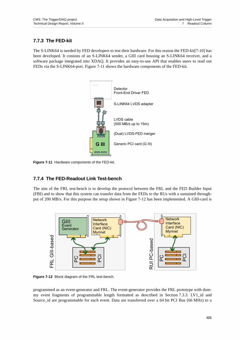
CMS: The Trigger/DAQ project Data Acquisition and High-Level TriggerTechnical Design Report, Volume II 7 Readout Column
7.7.3 The FED-kit
The S-LINK64 is needed by FED developers to test their hardware. For this reason the FED-kit[7-10] hasbeen developed. It consists of an S-LINK64 sender, a GIII card housing an S-LINK64 receiver, and asoftware package integrated into XDAQ. It provides an easy-to-use API that enables users to read outFEDs via the S-LINK64-port. Figure 7-11 shows the hardware components of the FED-kit.
7.7.4 The FED-Readout Link Test-bench
The aim of the FRL test-bench is to develop the protocol between the FRL and the FED Builder Input(FBI) and to show that this system can transfer data from the FEDs to the RUs with a sustained through-put of 200 MB/s. For this purpose the setup shown in Figure 7-12 has been implemented. A GIII-card is
programmed as an event-generator and FRL. The event-generator provides the FRL prototype with dum-my event fragments of programmable length formatted as described in Section 7.3.3. LV1_id andSource_id are programmable for each event. Data are transferred over a 64 bit PCI Bus (66 MHz) to a
Figure 7-11 Hardware components of the FED-kit.
Figure 7-12 Block diagram of the FRL test-bench.
DetectorFront-End Driver FED
(Dual) LVDS-FED merger
Generic PCI card (G III)
LVDS cable (500 MB/s up to 15m)
S-LINK64 LVDS adapter
G III
PC
NetworkInterface Card (NIC)Myrinet
PC
GIII: Event Generator
PCI
PCI
NetworkInterface Card (NIC)Myrinet
FRL
GIII
-bas
ed
RU
I PC
-bas
ed
121

CMS: The Trigger/DAQ project Data Acquisition and High-Level TriggerTechnical Design Report, Volume II 7 Readout Column
Myrinet network interface card which implements the FBI. The GIII card and NIC are housed in one PCand share the same PCI bus. On the receiver side the Myrinet interface card transfers the data over thePCI bus into the memory of a PC. The protocol between the FRL and the NIC card is discussed in the fol-lowing section.
7.7.4.1 Protocol Between the FRL and the Network Interface Card
The Myrinet NIC card contains a programmable RISC CPU. The on-board memory contains the programfor the RISC and serves as a buffer for the data to be transmitted. The PCI interface can be operated asmaster or slave.
As can be seen in Figure 7-4 the length of an event fragment is only stored at the end of the fragmentwhich makes it impossible for the FRL to determine if enough memory space for the entire fragment isavailable in the NIC. To solve this problem the protocol has been implemented using a “buffer-loan-ing”-scheme based on the technique described in Section 11.2.3, "Memory Management": the buffermemory of the NIC is divided into blocks of fixed size. Each block contains reserved space for a Myrinetheader, the FRL header, and the data payload. The following steps are executed during operation:
1. As soon as there is a free memory block available, the NIC writes its address into a FIFO in theFRL. At start-up all blocks are available. During operation a block becomes available after the datait contained has been sent successfully over the Myrinet link.
2. As soon as there are pointers to free blocks in the FIFO, an event is generated. In this test-benchsetup, the parameters of the event fragments to be generated (length, LV1_id, Source_id) musthave been written previously into a second FIFO by the control software. The generated event istransferred by the FRL via a DMA directly into the payload area of the memory block. The FRLheader for this block is written afterwards. If the fragment is too large to fit into one memory block,a special flag in the FRL header indicates that the fragment is continued in the next block. Step 2 isrepeated until the whole fragment has been written into the NIC buffer memory.
3. The control process in the NIC monitors the headers which are filled by the FRL. As soon as a flagtherein indicates the presence of a new block, it starts to fill the reserved space for the Myrinetheader and subsequently sends out the block over the optical link. After successful transmissionthe block is freed by setting the fragment length to 0. Its address is written into the FRL FIFO.
7.7.4.2 Measurements and Results
Two different measurements have been performed with this test-bench. In order to measure the overheaddue to the protocol introduced by the FRL, the first measurement was taken with the FRL prototypeplugged into a PC without any further hardware. A control program in the PC implemented the protocoldescribed above. In this configuration the overhead due to the control program of the PC is negligible.The data throughput on the PCI bus has been measured as a function of the fragment size (seeFigure 7-13). The asymptotic limit for a large fragment size is measured to be 500 MB/s which is close tothe theoretical limit of 528 MB/s for the PCI bus. The block size was set to 4 kB. A sawtooth structure isobserved since every time a new block is needed to transfer a complete fragment, additional overhead isintroduced in order to set up the DMA transfer for the block. This overhead, which has been measured tobe 0.6 µs, limits the total data throughput to 500 MB/s.
In a second measurement, the complete chain described above was set up. Details of this measurement aredescribed in Section 6.4.4.3.2, "Building of Super-fragments".
122

CMS: The Trigger/DAQ project Data Acquisition and High-Level TriggerTechnical Design Report, Volume II 7 Readout Column
7.7.5 The Readout Unit Test-bench
A Readout Unit test-bench has been set up, in order to measure the data throughput of the RU under real-istic conditions. The functional diagram is shown in Figure 7-14. The Readout Unit is implemented by aPC with at least two 64 bit / 66 MHz PCI slots. The RU-input (RUI), implemented by a GIII card, pushesdata into the RU. At the output, data are transferred first to a NIC, which functions as a RUO, and fromthere to the Builder Unit (BU). The BU checks the incoming data for correctness.
The setup contains a data generator and a trigger emulator. The trigger emulator accepts veto signals tosimulate the Trigger-Throttling System (TTS). Both the Event Manager (EVM) and the data generatorcan send a veto to the trigger emulator. The event generator is contained in the RUI and generates anevent on receipt of each Level-1 Trigger. The distribution of the event-size is programmable. The generat-ed event is fed into the RU via the PCI bus of the host PC.
The data and the control messages of the event builder protocol are sent over a Myrinet network. The pro-tocol used is GM, developed by Myricom.
The software of the test-bench is written in the XDAQ framework which is described in Chapter 10. Thebuffer-loaning scheme described above (see Section 7.7.4) prevents the loss of data in case of buffershortage in the RU. Different event building protocols between RU, BU and EVM can be tested in the set-up. All measurements presented in the next section were performed using a variant of the event buildingprotocol described in Section 5.3.2.1, "Event Flow Protocols", currently implemented in XDAQ. This isnot expected to affect the results on throughput described hereafter.
7.7.5.1 Measurements and Results
As can be seen in Figure 7-14, the control messages are sent over the same network as the data. In orderto reduce the network load due to control messages, their number is reduced by bundling the “send toBU” messages from the EVM to the RU: a single message contains the request for 50 event fragments.The same method has been applied for the “resource available” messages of the BU to the EVM.
Figure 7-13 Performance of the FRL PCI interface: throughput as a function of the fragment size. A GIII-basedFRL is plugged into a PC which runs a control program implementing the protocol discussed in the text.
FED fragment size [Bytes]
0
100
200
300
400
500
600
0 1000 2000 3000 4000 5000 6000 7000 8000 9000 10000
PCI 64b/66MHz 528 MB/sFRL-PCI
Thro
ughp
ut [M
B/s
]
123
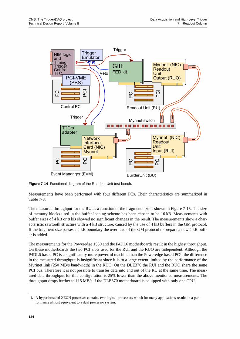
CMS: The Trigger/DAQ project Data Acquisition and High-Level TriggerTechnical Design Report, Volume II 7 Readout Column
Measurements have been performed with four different PCs. Their characteristics are summarized inTable 7-8.
The measured throughput for the RU as a function of the fragment size is shown in Figure 7-15. The sizeof memory blocks used in the buffer-loaning scheme has been chosen to be 16 kB. Measurements withbuffer sizes of 4 kB or 8 kB showed no significant changes in the result. The measurements show a char-acteristic sawtooth structure with a 4 kB structure, caused by the use of 4 kB buffers in the GM protocol.If the fragment size passes a 4 kB boundary the overhead of the GM protocol to prepare a new 4 kB buff-er is added.
The measurements for the Poweredge 1550 and the P4DL6 motherboards result in the highest throughput.On these motherboards the two PCI slots used for the RUI and the RUO are independent. Although theP4DL6 based PC is a significantly more powerful machine than the Poweredge based PC1, the differencein the measured throughput is insignificant since it is to a large extent limited by the performance of theMyrinet link (250 MB/s bandwidth) in the RUO. On the DLE370 the RUI and the RUO share the samePCI bus. Therefore it is not possible to transfer data into and out of the RU at the same time. The meas-ured data throughput for this configuration is 25% lower than the above mentioned measurements. Thethroughput drops further to 115 MB/s if the DLE370 motherboard is equipped with only one CPU.
Figure 7-14 Functional diagram of the Readout Unit test-bench.
1. A hyperthreaded XEON processor contains two logical processors which for many applications results in a per-formance almost equivalent to a dual processor system.
PC PCI
PCPC
Readout Unit (RU)
Myrinet switch
BuilderUnit (BU)Event Mananger (EVM)
PC PCI
Control PC
NIM logicandTimingTriggerControlTTC
Myrinet (NIC)ReadoutUnit Output (RUO)
GIII: FED kit
Trigger
Trigger
Veto
PCI
PCI
Myrinet (NIC)ReadoutUnit Input (RUI)
TTCrxadapter
NetworkInterface Card (NIC)Myrinet
TriggerEmulator
PCI-VME(SBS)
124

CMS: The Trigger/DAQ project Data Acquisition and High-Level TriggerTechnical Design Report, Volume II 7 Readout Column
A similar measurement is shown in Figure 7-16. Here the fragment sizes are varied according to alog-normal distribution. The rms of the distribution has been set to its mean divided by 1.The variationof the event size smears out the characteristic sawtooth structure of the previous measurements. For amean event size of 16 kB, a data throughput of 205 MB/s is measured for the P4DL6-based PC and
Table 7-8 Important characteristics of the PCs used to implement the RU in the Readout Unit test-bench. ThePCs are based on motherboards of two vendors: SuperMicro and DELL.
SuperMicro SuperMicro DELL SuperMicro
Motherboard DLE 370 DLE370 Powerdege 1550 P4DL6
Chipset vendor ServerWorks ServerWorks ServerWorks ServerWorks
ChipsetServerSet III-LE ServerSet III-LE
ServerSet III HE-SE-SL
Grand Champion LE
CPU1 Pentium III 2 Pentium III 2 Pentium III
1 Pentium IV Xeon (hyperthreaded)
CPU clock 1 GHz 1 GHz 930 MHz 2.0 GHz
Memory
SDRAM(1.06 GB/s)
SDRAM(1.06 GB/s)
SDRAM (interleaved)(2.12 GB/s)
DDR SDRAM (interleaved)(3.2 GB/s)
System Bus 1.06 GB/s 1.06 GB/s 1.06 GB/s 3.2 GB/s
PCI 64 bit / 66 MHZ slots
2 slots on 1 bus 2 slots on 1 bus2 slots on independent buses
4 slots on 2 inde-pendent buses
Figure 7-15 Data throughput measured in the RU as a function of the fragment size. Each measurement hasbeen performed with fixed fragment size. The measurements have been performed with 4 different PCs (seetext).
1. This is motivated by naively assuming that each 16 kB fragment has been assembled in the FED Builder out of 82-kB fragments. For each of these fragments a size distribution according to a log normal distribution with an rmsequivalent to its mean is assumed.
Thro
ughp
ut [M
B/s
]
0
50
100
150
200
250
0 16 32 48 64 80Fragment size [kB]
Dell Poweredge 1550 (2 CPUs)SuperMicro 370 DLE (2 CPUs)SuperMicro 370 DLE (1 CPU)SuperMicro P4DL6
8
125
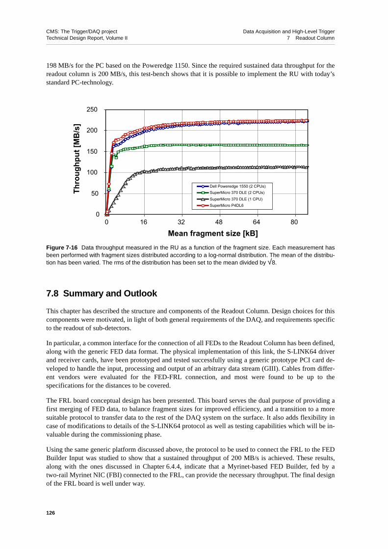
CMS: The Trigger/DAQ project Data Acquisition and High-Level TriggerTechnical Design Report, Volume II 7 Readout Column
198 MB/s for the PC based on the Poweredge 1150. Since the required sustained data throughput for thereadout column is 200 MB/s, this test-bench shows that it is possible to implement the RU with today’sstandard PC-technology.
7.8 Summary and Outlook
This chapter has described the structure and components of the Readout Column. Design choices for thiscomponents were motivated, in light of both general requirements of the DAQ, and requirements specificto the readout of sub-detectors.
In particular, a common interface for the connection of all FEDs to the Readout Column has been defined,along with the generic FED data format. The physical implementation of this link, the S-LINK64 driverand receiver cards, have been prototyped and tested successfully using a generic prototype PCI card de-veloped to handle the input, processing and output of an arbitrary data stream (GIII). Cables from differ-ent vendors were evaluated for the FED-FRL connection, and most were found to be up to thespecifications for the distances to be covered.
The FRL board conceptual design has been presented. This board serves the dual purpose of providing afirst merging of FED data, to balance fragment sizes for improved efficiency, and a transition to a moresuitable protocol to transfer data to the rest of the DAQ system on the surface. It also adds flexibility incase of modifications to details of the S-LINK64 protocol as well as testing capabilities which will be in-valuable during the commissioning phase.
Using the same generic platform discussed above, the protocol to be used to connect the FRL to the FEDBuilder Input was studied to show that a sustained throughput of 200 MB/s is achieved. These results,along with the ones discussed in Chapter 6.4.4, indicate that a Myrinet-based FED Builder, fed by atwo-rail Myrinet NIC (FBI) connected to the FRL, can provide the necessary throughput. The final designof the FRL board is well under way.
Figure 7-16 Data throughput measured in the RU as a function of the fragment size. Each measurement hasbeen performed with fragment sizes distributed according to a log-normal distribution. The mean of the distribu-tion has been varied. The rms of the distribution has been set to the mean divided by √8.
0
50
100
150
200
250
0 16 32 48 64 80
Mean fragment size [kB]
Thro
ughp
ut [M
B/s
]
Dell Poweredge 1550 (2 CPUs)SuperMicro 370 DLE (2 CPUs)SuperMicro 370 DLE (1 CPU)SuperMicro P4DL6
126

CMS: The Trigger/DAQ project Data Acquisition and High-Level TriggerTechnical Design Report, Volume II 7 Readout Column
The main requirement placed on the Readout Unit is the concurrent read/write access to memory, with athroughput of 200 MB/s. A custom hardware solution has been made obsolete by the availability of com-mercial personal computers which can meet this I/O requirements. As a consequence the prototype activ-ity has concentrated on maximizing the exploitation of the memory bandwidth by means of DMA datatransfers for input and output, using an efficient memory management based on buffer-loaning. The pro-totype software has been tested in a dedicated setup, on several different personal computers. The twomost recent machines used in the test can both provide the necessary throughput.
In conclusion, for all the components of the Readout Column, an implementation that can meet the re-quirements has been identified and tested. The design of the custom components that have to be installedin the underground area is being finalized and the following production phase is expected to meet the in-stallation deadlines. Further tests of the production design, as well as integration tests of all the compo-nents in a complete Readout Column, are planned.
7.9 References
7-1 B.G. Taylor, “TTC Distribution for LHC Detectors”, IEEE Trans. Nucl. Sci., 45 (1998) 82;B.G. Taylor,”Timing Distribution at the LHC”, in Proceedings of the 8th Workshop on Electronics for LHC Experiments, Colmar, France, 9-13 September 2002, pp. 63-74.Timing Trigger and Control system, see http://www.cern.ch/TTC/intro.htm.
7-2 A. Racz, R. McLaren, E. van der Bij, “The S-LINK64 bit extension specification: S-LINK64”, available at http://hsi.web.cern.ch/HSI/s-link; O. Boyle, R McLaren, E. van der Bij, “The S-LINK Interface Specification”, available at http://hsi.web.cern.ch/HSI/s-link
7-3 CMS Coll.,“The Trigger and Data Acquisition project, Volume I, The Level-1 Trigger, Technical Design Report”, CERN/LHCC 2000-038, CMS TDR 6.1, 15 December 2000.
7-4 Technical Design Reports of the CMS sub-detectors:CMS Coll.,“The Tracker Project, Technical Design Report”, CERN/LHCC 98-6, CMS TDR 5, 15 April 1998Tracker Addendum - CERN/LHCC 2000-016, CMS TDR 5 Addendum 1, 21 February 2000CMS Coll.,“The Electromagnetic Calorimeter Project, Technical Design Report”, CERN/LHCC 97-33, CMS TDR 4, 15 December 1997CMS Coll.,“The Hadronic Calorimeter Project, Technical Design Report”, CERN/LHCC 97-31, CMS TDR 2, 20 June 1997CMS Coll.,“The Muon Project, Technical Design Report”, CERN/LHCC 97-32, CMS TDR 3, 15 December 1997
7-5 S. Cittolin, J.F. Gillot, A. Racz, “Front-end logical model in CMS”, CMS Technical Note 1996/015.
7-6 A. Racz ,”Trigger throttling system for CMS DAQ”, in Proceedings of the 6th Workshop on Electronics for LHC Experiments, Cracow, Poland, 11-15 September 2000, pp. 405-409.
7-7 N. Marinelli, “APV logic simulations”, CMS Note 1999/028.
7-8 CMS DAQ Readout Unit Working Group, see http://cmsdoc.cern.ch/cms/TRIDAS/horizontal
7-9 O. Kodolova, I. Tomalin and P. Yepes, “Expected Data Rates from the Silicon Strip Tracker”, CMS Note-2002/047.
7-10 E. Cano et al. “FED-kit design for CMS DAQ system”, in Proceedings of the 8th Workshop on Electronics for LHC Experiments, Colmar, France, 9-13 September 2002, pp. 274-277.
127

CMS: The Trigger/DAQ project Data Acquisition and High-Level TriggerTechnical Design Report, Volume II 7 Readout Column
128
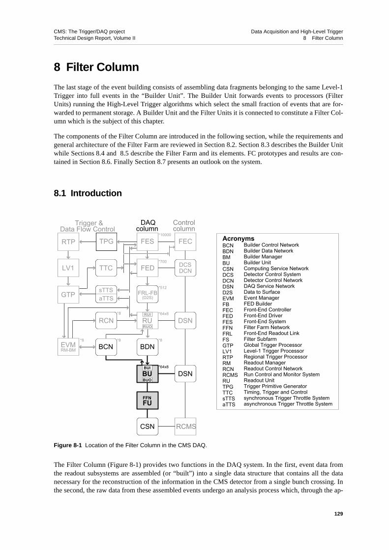
CMS: The Trigger/DAQ project Data Acquisition and High-Level TriggerTechnical Design Report, Volume II 8 Filter Column
8 Filter Column
The last stage of the event building consists of assembling data fragments belonging to the same Level-1Trigger into full events in the “Builder Unit”. The Builder Unit forwards events to processors (FilterUnits) running the High-Level Trigger algorithms which select the small fraction of events that are for-warded to permanent storage. A Builder Unit and the Filter Units it is connected to constitute a Filter Col-umn which is the subject of this chapter.
The components of the Filter Column are introduced in the following section, while the requirements andgeneral architecture of the Filter Farm are reviewed in Section 8.2. Section 8.3 describes the Builder Unitwhile Sections 8.4 and 8.5 describe the Filter Farm and its elements. FC prototypes and results are con-tained in Section 8.6. Finally Section 8.7 presents an outlook on the system.
8.1 Introduction
The Filter Column (Figure 8-1) provides two functions in the DAQ system. In the first, event data fromthe readout subsystems are assembled (or “built”) into a single data structure that contains all the datanecessary for the reconstruction of the information in the CMS detector from a single bunch crossing. Inthe second, the raw data from these assembled events undergo an analysis process which, through the ap-
Figure 8-1 Location of the Filter Column in the CMS DAQ.
RTP FECTPG
TTC
sTTSaTTSGTP
LV1 FED
FES
DCS
RU
EVMRM-BM
BU
FFNFU
BDN
DCN
DSN
RCMSCSN
DSNRCN
BCN
*700
*10000
*512
*8*8*8
*8 *64x8
*64x8
RUI
RUO
BUI
BUO
DAQ ControlTrigger &column columnData Flow Control
FRL-FB(D2S)
AcronymsBCNBDNBMBUCSNDCSDCNDSND2SEVMFBFECFEDFESFFNFRLFSGTPLV1RTPRMRCNRCMSRUTPGTTCsTTSaTTS
Builder Control NetworkBuilder Data NetworkBuilder ManagerBuilder UnitComputing Service NetworkDetector Control SystemDetector Control NetworkDAQ Service NetworkData to SurfaceEvent ManagerFED BuilderFront-End ControllerFront-End DriverFront-End SystemFilter Farm NetworkFront-End Readout LinkFilter SubfarmGlobal Trigger ProcessorLevel-1 Trigger ProcessorRegional Trigger ProcessorReadout ManagerReadout Control NetworkRun Control and Monitor SystemReadout UnitTrigger Primitive GeneratorTiming, Trigger and Control synchronous Trigger Throttle Systemasynchronous Trigger Throttle System
129

CMS: The Trigger/DAQ project Data Acquisition and High-Level TriggerTechnical Design Report, Volume II 8 Filter Column
plication of reconstruction and filtering algorithms, referred to as the High-Level Trigger (HLT), leads toa decision on whether to reject the event or to keep it for offline analysis. The events rejected by the HLTare discarded, whereas the events accepted are transferred to the Computing Services (see Chapter 16,"Computing Services") for permanent storage.
The Filter Column (FC) represents a “vertical slice” of the system, which is functionally split into twounits, namely the Builder Unit (BU) and the Filter Unit (FU). The Builder Unit is part of the Event Build-er, and its functionality is to provide the event assembly. It is thus tightly coupled to the architecture of thedata network and the readout. The Filter Unit is the basic element on which the HLT algorithms are exe-cuted. It is a unit which is presented, by the BU, with fully assembled events and thus its functionality isindependent of the details of the Event Builder. The entire collection of Filter Units is referred to as the“Filter Farm”.
8.2 Filter Farm Requirements and Architecture
The CMS Filter Farm consists of a large number, of O(103), of processors. The farm is organised in anumber of smaller subfarms each with ~100 processors (see Figure 8-2). This organization has numerousadvantages, since:
• it allows for a staged deployment of the total computational power required
• it introduces a natural hierarchical structure to the farm, simplifying its management by fa-cilitating the dispatching of control, monitor, and error messages.
• it improves the robustness and fault tolerance of the system by making it possible to keepthe output streams separated at the level of each subfarm, thus decreasing the risk of dataloss (and experiment deadtime) due to unavailability or fault in the central data storage serv-ices.
Each subfarm corresponds to one or more BUs connected to one or more of the Builder Data Network(BDN) output ports, and comprises a number of FUs. The BUs of a single subfarm belong to the same RU
Figure 8-2 Filter Farm and the Event Builder (top) and the subfarm structure (bottom).
Filte
r Sub
Farm
BuilderUnits
EventManager ControlsReadout Unit Builder (64x64)
FilterSub-farms
BU
Filter Farm Networks
FU
FU FU FU SM
Filter Data Network (FDN)
Filter Control Network (FCN)
130

CMS: The Trigger/DAQ project Data Acquisition and High-Level TriggerTechnical Design Report, Volume II 8 Filter Column
Builder. A FU may correspond to a physical unit of computation (e.g. a PC) or to a logical unit in a morecomplex system consisting of several computational units (e.g. a multi-cpu server). In a subfarm, the FUsare connected to the BUs via a Filter Data Network (FDN). A Special node called Subfarm Manager (SM)handles the distribution of code, configuration and control commands to all the FUs as well as the collec-tion of monitor data. It is connected to the FUs via the Filter Control Network (FCN). The FDN and FCNare collectively referred to as Filter Farm Networks.
The requirements on the performance of the filter farm are particularly tight. The farm must cope with thefull event rate accepted by the Level-1 Trigger, i.e. an aggregate event rate of up to 100 kHz. Moreover,the rate of events output to storage is O(102) Hz and thus the HLT algorithms must achieve a rejectionfactor of O(103). A subfarm spanning n BUs of the N available must sustain an event rate up to n/N × 105
Hz, which corresponds to a mean time of N/n × 10-5 s per event. Using, as indicative figures, the valuesN=512 and n=8, we conclude that each subfarm must handle ~1.5 kHz of events, or a mean of 0.64 ms perevent. Irrespective of the size of the subfarm, a single BU must handle a rate up to 200 Hz, at 5 ms/event.
Each of the FU nodes is connected to the BUs via a network link. The time available for a FU to processan event is proportional to the number of FUs per BU. A variable number of FUs per BU will therefore bedeployed depending on the performance of a unit. The minimal amount of connectivity to fit a uniquecorrespondence between a BU and its FUs is driven by the maximum number of FUs per BU to be de-ployed. This connectivity must be guaranteed by a switched network. To allow dynamic, partial or fullreconfigurability of a subfarm, a larger fabric is necessary.
The above throughput requirements imply either the usage of multi-gigabit/s links for the BU-FU connec-tion, or the employment of additional techniques to reduce the traffic of data between the two units. Anexample of such a technique is the possibility to transfer events between the BU and FU only partially, ona “need” basis. Since the actual filtering process is performed in steps, and each step uses typically only asubset of the event data and results in the rejection of numerous events, one can envisage the transfer ofthe event data from the BU to the FU in multiple steps, each step containing only the data necessary forthe next filtering algorithm. We illustrate this procedure using a simple two-stage filter which consists oftwo “trigger algorithms”, called symbolically “Level-2” and “Level-3”, in complete analogy with the trig-ger levels of traditional DAQ systems. Suppose that the Level 2 decision can be based on only 1/4 of thetotal event data (e.g. the data from the calorimeter and muon detectors), and that results in the rejection ofO(90%) of the input events. At an average event size of 1 MB, the average amount of data to be trans-ferred by a single BU to the nodes of a subfarm is only ~70 MB/s, compared to the 200 MB/s that wouldcorrespond to the transfer of the full data for each event. The figures of the example used are taken frommeasurements using simulations of physics events in the CMS detector. In general, the amount ofprocessing to be performed to reach a decision can be minimised by only reconstructing regions of the de-tector corresponding to interesting features of the event. These regional reconstruction can help to furtherreduce the fraction of data to be transferred for a certain detector, if the readout segmentation convenient-ly maps typical regions of interest. A more detailed discussion of the data needed for each filtering step,regional reconstruction, and the associated performance of each algorithm can be found in Chapter 15,"Physics Object Selection and HLT Performance".
Although the Builder Units may absorb processing time fluctuations, the Filter subfarm must keep upwith the BU input rate at “equilibrium”. To ensure the scalability and seamless evolution of the system,the FU software implementation must clearly be made as platform independent as possible, allowing amixed operating system / hardware architecture scenario. However, the level of portability is expected tobe determined by the reconstruction software and related products.
The aggregate output of an individual subfarm is the aggregate accept rate (n × 0.2 Hz, where n is thenumber of BUs per subfarm) times the average size of an output event, which for contingency we can as-sume to be ~ 1.5 MB1. The amount of output storage needed by a single subfarm with n = 8 and over 24
131

CMS: The Trigger/DAQ project Data Acquisition and High-Level TriggerTechnical Design Report, Volume II 8 Filter Column
hours of data taking is therefore ~ 200 GB. The corresponding average number of transactions per secondto such a storage is small compared to the Farm total. To allow the Filter Farm to continue working whilee.g. the connection to the Computing Services is unavailable (see Section 16.2), it is convenient to pro-vide local mass storage on an individual node of the subfarm, (which can be physically the same as theSubfarm Manager), to store accepted events. Subsequent transfers to the Computing Services can be con-veniently sized and scheduled, e.g. on a run-by-run or fill-by-fill basis. In case of failure of a subfarm,causing local data corruption, the amount of lost data is also minimized.
When data taking is first started, or after power off of the whole farm, a “cold start” must be initiated. Thecold start includes booting and configuration of all the machines in the farm, download of new softwareand bootstrap of the relevant DAQ daemons on the FU nodes, and of server software on the SubfarmManagers. The cold start is managed by the Farm Control under the supervision of the main Run Controlsystem. In order not to cause experiment dead time, the cold start time must be negligible on the timescale of the setup time of the LHC beam. At the end of a cold start the farm is ready to be configured andstarted, which is the normal condition between machine fills. The configuration and starting of all theprocesses in the farm, which leads to the farm being ready to take data, is referred to as a “warm start”.The warm start time must be negligible with respect to the interval between two machine fills. The hierar-chical structure of the farm is meant to minimize the cold start time by parallelizing the software distribu-tion and the execution of configuration commands on all the nodes. The distribution of control commandsneeded to start data taking on the farm once it is configured, exploit the same hierarchical structure,whereby individual nodes are controlled and report their status to the relevant Subfarm Manager, which inturn responds to commands from Run Control. This hierarchical structure is outlined in more detail inSection 8.5.
The farm monitoring must guarantee reliable delivery of alarm messages which have system wide scopeor require operator intervention, with a delay which is small compared to the reaction time of the systemor operator. Provisions must be made to allow for alarm masking and resetting. Monitoring of workingparameters must guarantee timely delivery of monitor information. For sampled monitor information (e.g.event display), sampling of all the nodes according to a “fair share” policy must be guaranteed. The datathroughput required for update of monitor information to the monitor clients is expected to be consistentwith what can be provided by a commercial “office” network.
The farm is operated as a collection of independent subfarms. Different subfarms can be assigned to dif-ferent partitions, and failure of a subfarm in a partition will not affect the performance of the other sub-farms. Within a subfarm, FU nodes are only coupled insofar as they depend on the same BU for theirinput. Therefore, in principle, a subfarm can also be partitioned. Failure of one or more FUs hanging froma given BU will cause that BU to work at a lower event rate. If “more graceful” performance deteriorationis required, dynamic reconfiguration of FU assignments must be guaranteed by appropriate switching ca-pabilities in the FDN.
8.3 Builder Unit (BU)
The task of the Builder Unit is to retrieve data from the RUs in the form of event “super-fragments” (seeSection 4.2), to assemble these super-fragments into full events, and to send data from assembled eventsto FUs upon request. The BU is connected, as shown in Figure 8-3, to the Readout Units (RU) and the Fil-
1. Throughout this Technical Design Report, an average size of 1 MB for the raw event is assumed. Here, provisionis made for the possibility to attach to the raw event additional information which is the result of the reconstructionand analysis carried out during the selection.
132
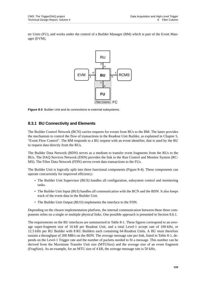
CMS: The Trigger/DAQ project Data Acquisition and High-Level TriggerTechnical Design Report, Volume II 8 Filter Column
ter Units (FU), and works under the control of a Builder Manager (BM) which is part of the Event Man-ager (EVM).
8.3.1 BU Connectivity and Elements
The Builder Control Network (BCN) carries requests for events from BUs to the BM. The latter providesthe mechanism to control the flow of transactions in the Readout Unit Builder, as explained in Chapter 5,"Event Flow Control". The BM responds to a BU request with an event identifier, that is used by the BUto request data directly from the RUs.
The Builder Data Network (BDN) serves as a medium to transfer event fragments from the RUs to theBUs. The DAQ Services Network (DSN) provides the link to the Run Control and Monitor System (RC-MS). The Filter Data Network (FDN) serves event data transactions to the FUs.
The Builder Unit is logically split into three functional components (Figure 8-4). These components canoperate concurrently for improved efficiency:
• The Builder Unit Supervisor (BUS) handles all configuration, subsystem control and monitoringtasks.
• The Builder Unit Input (BUI) handles all communication with the BCN and the BDN. It also keepstrack of the event data in the Builder Unit.
• The Builder Unit Output (BUO) implements the interface to the FDN.
Depending on the chosen implementation platform, the internal communication between these three com-ponents relies on a single or multiple physical links. One possible approach is presented in Section 8.6.1.
The requirements on the BU interfaces are summarized in Table 8-1. These figures correspond to an aver-age super-fragment size of 16 kB per Readout Unit, and a total Level-1 accept rate of 100 kHz, or12.5 kHz per RU Builder with 8 RU Builders each containing 64 Readout Units. A BU must thereforesustain a throughput of 200 MB/s on the BDN. The average message rate per link, listed in Table 8-1, de-pends on the Level-1 Trigger rate and the number of packets needed to fit a message. This number can bederived from the Maximum Transfer Unit size (MTUSize) and the average size of an event fragment(FragSize). As an example, for an MTU size of 4 kB, the average message rate is 50 kHz.
Figure 8-3 Builder Unit and its connections to external subsystems.
FU
EVM
RU
RCMS
FC
BU
Filter Column
1
11
n
n
n
n
n
133

CMS: The Trigger/DAQ project Data Acquisition and High-Level TriggerTechnical Design Report, Volume II 8 Filter Column
For the BCN port, a large number of messages can be packed in a single physical transfer since the mes-sages are small. Each BU sends requests for new events at a rate of 200 Hz. It also receives confirmationsand sends out clear messages at the same rate, resulting in a total message rate to and from the EventManager of 600 Hz. Assuming a typical message size (indicated with MsgSize in the table) of 100 B, anaverage throughput of 60 kB/s is required. This traffic is negligible compared to that required for thecommunication with the Readout Units (in parentheses in the table). Event requests to RUs must be sentto 64 destinations, for a total rate of 12.5 kHz. If needed, this rate can be reduced by appropriate messagegathering. The required throughput is of the order of 1 MB/s.
The load of the FDN at the BU output depends on the FU operational mode. As already mentioned, thetransfer of full events requires an aggregate output bandwidth of 200 MB/s. If multi-step filtering is used,as outlined in Section 8.2 above, this bandwidth can decrease significantly. The message rate at this port,however, is increased of a fraction equivalent to the fraction of events accepted by the first filtering step.
The BU internal communication capabilities have to meet the BDN, the BCN and the FDN port require-ments. A single shared interconnect must sustain an aggregate throughput of BUI and BUO of 400 MB/s.The bandwidth to the event data memory must exceed 400 MB/s.
Figure 8-4 Builder Unit internals and network connectivity.
Table 8-1 Requirements on the BU network interfaces. The message rates are parametrized by the MaximumTransfer Unit size (MTUSize) for the switched network.
BDN BCN DSN FDN
Average throughput
200 MB/s<< 1 MB/s(~ 1 MB/s)
< 1 MB/s200 MB/s(70 /s)
Average message rate
< 1 kHz ~ 600 Hz
Traffic type
event building
event building control
configuration, con-trol, monitoring
event filtering
EVMRM-BM
BU
FFNFU
BDN
DSN
RCMSCSN
BCN
BUI
BUOAcronymsBCNEVMBMBDNBUBUIBUOBUSFFNFUCSN
Builder Control NetworkEvent ManagetBuilder ManagerBuilder Data NetworkBuilder UnitBuilder Unit InputBuilder Unit OutputBuilder Unit SupervisorFilter Farm NetworkFilter UnitComputing Service Network
BU
S
1-10 MB/s
1-10 MB/s
200 MB/s
200 MB/s
1-10 MB/s
12.5kHzFragSizeMTUSize----------------------- 12.5kHz
MsgSizeMTUSize-----------------------
134

CMS: The Trigger/DAQ project Data Acquisition and High-Level TriggerTechnical Design Report, Volume II 8 Filter Column
8.3.2 Data Flow
The protocol used by the BUI to communicate with the RU and the EVM is discussed in Section 5.3.2.1,"Event Flow Protocols" and in more detail in Appendix C, "Event Flow Control Protocols in RU Build-er". In summary, the BU requests a new event of a given type from the Event Manager. The Event Manag-er then allocates an event to the BU and returns an Event Identifier. Subsequently, the BU requests datafrom all the RUs. Once the event is assembled, it can be allocated to a Filter Unit in response to a requestfor a new event, at which point the BU informs the Event Manager that all resources associated with thisevent can be liberated.
The BUI accepts messages from the Event Manager containing newly allocated Event Identifiers, andmessages with super-fragment data from the Readout Units. The Builder Unit Output accepts two types ofrequests from the Filter Unit: requests to allocate new events by event type, and requests for sets of eventsuper-fragments. A set comprises a configurable number of Readout Units. A Filter Unit can retrievemore data for a certain event until it decides to discard the event1. If an event is discarded, the BuilderUnit releases all internal resources associated with it.
The BUO interface is used by the FU to allocate new events, using the allocate message, and to retrievemore data for an allocated event, using the collect message. In both cases, the BUO delivers the requesteddata to the FU using the take message. The FU sends a discard message to the BUO when the event hasbeen rejected or sent to storage.
The internal interface between Builder Unit Input (BUI) and Output (BUO) comprises five functions,three belonging to the BUI and two to BUO. The interaction diagram for the builder unit internal commu-nication is shown in Figure 8-5. The BUO asks the BUI to build an event of a given type. The BUI re-
sponds to this request by informing the BUO as soon as the event is ready for delivery, also providing theresource identifier that a Filter Unit uses subsequently as an identifier for this event. The BUO forwardssubsequent requests for event fragment sets from Filter Units to the BUI using its retrieve interface
1. This protocol is designed to allow multi-step transfer of events to the Filter Unit. However, should the FDN con-nectivity allow it, the same protocol can be used to transfer entire events with a single request message.
Figure 8-5 Communications among the Builder Unit elements.
BUO BUI
allocate by event typewith initial fragment set
retrieve fragment set
retrieve fragment set
data for fragment set
deliver to FU
resource is ready
allocate by event type
BUResource pool
135

CMS: The Trigger/DAQ project Data Acquisition and High-Level TriggerTechnical Design Report, Volume II 8 Filter Column
(Figure 8-6). The BUI replies to this requests with the data message that contains all necessary informa-tion to send the data to a filter unit. To release all resources that are associated with an event in the BUI,the BUO uses the clear command. A FU cannot request more fragment sets for an event after it has issueda discard.
8.3.3 Control and Monitor
A Builder Unit is controlled, configured and monitored by the Run Control and Monitor System (RCMS).In the case of the BU there are two types of configuration parameters, those relevant to the networkingenvironment and those relevant to the operation of the system. The operational parameters are listed inTable 8-2.
The minimal monitoring capabilities of the builder unit comprise:
• Occupancy of the resource pool.
• Event building rate
• Binary dump of all event fragments for a given resource.
• Error counts (by event, by resource, etc.)
Operational anomalies are reported to the run control system. Internally, they are classified according totheir severity. Warnings are occurrences that may subsequently lead to a failure. A failure requires exter-nal intervention to recover. In this case, it will be possible to store all the information relative to the cur-rent state of the application with the monitoring service.
Figure 8-6 Subsequent requests for fragment sets.
Table 8-2 Builder Unit configuration: operational parameters.
Name Purpose
Maximum number of events Determines the BU memory resources
Fragment set definitions Mapping of fragment set identifiers to collections of RU identifiers
Event type definitions Mapping of identifiers to event types
Request gathering Number of requests gathered in a packet for a given network
BUO BUI
retrieve fragmentset by builder unitresource identifier
retrieve fragment set
clear
retrieve fragment set
data for fragment setdeliver to FU
discard event
BUResource pool
136

CMS: The Trigger/DAQ project Data Acquisition and High-Level TriggerTechnical Design Report, Volume II 8 Filter Column
Errors in the communication with the rest of the Event Builder are described in detail in Section 9.2.2.5.A fault tolerance analysis of the BU-FU protocol is presented in Section 9.2.3. For the communicationwith RCMS, reliable delivery is assumed. The BU must be capable of continuing its operation in case theconnection to the RCMS is lost.
8.4 Filter Unit (FU)
A Filter Unit node is an elementary computational unit of the Filter Farm, i.e. it is either one PC or oneCPU in a CPU server. Its local resources (e.g. memory and disk space) are limited, but in general it alsohas access to external shared resources. It is part of a distributed computing environment consisting of theFilter Farm, the Run Control and Monitoring System, and the Computing Services. Shared resources in-clude boot servers, configuration and file servers, and databases containing software, configurations, con-ditions and other data.
The Filter Unit connects to two logically distinct networks (see Figure 8-7): the FDN, which connects itto the BU, and the FCN, which connects it to the Subfarm Manager. The FU makes indirect transactionsto the Computing Services and Run Control System through the Subfarm Manager (SM), which, via theCSN, connects to the central computing and storage facilities (see Chapter 16, "Computing Services").
8.4.1 FU Functionality and Elements
The Filter Unit software consists of application components which fit in the layered scheme of the Onlinesoftware outlined in Section 3.3, "Software Architecture" and discussed in more depth in Chapter 10.
There are four main software components in the FU, illustrated, along with their relationships, inFigure 8-8:
• The Filter Framework which embeds all the FU data access and control layers.
• The Filter Tasks which run HLT algorithms and perform the event selection in the context of theframework. An HLT task allocates an event, reads sets of fragments from that event, processesthese data and finally closes the event.
Figure 8-7 Filter Unit and its connections to other DAQ and external subsystems.
Filter Column
mn
1n
1n
1n
BU
FU
RCMS
CSN
AcronymsBUBUIBUOBUSFUSMCSNRCMS
Builder UnitBuilder Unit InputBuilder Unit OutputBuilder Unit SupervisorFilter UnitSubFarm ManagerComputing Service NetworkRun Control and Monitor System
SM
137

CMS: The Trigger/DAQ project Data Acquisition and High-Level TriggerTechnical Design Report, Volume II 8 Filter Column
• The Filter Unit Monitor, which, in conjunction with the framework, provides a consistent interfacefor monitoring of system-level and application-level parameters of the Filter Unit. In particular, ithandles monitorable parameters of the HLT Tasks and status information of the FU, collects andelaborates statistical data which are delivered to the relevant consumers via the FCN.
• The Storage Manager which handles the transfer of event data out of the FU. An event accepted bythe HLT task remains inside the FU framework until its data have been transferred to a persistentstorage.
The following sections contain more details on the four components of the Filter Unit.
8.4.1.1 Filter Unit Framework
The Filter Unit framework provides two major functionalities: it receives and dispatches messages fromand to the BU, and coordinates the operation of the Filter Tasks by handling configuration and controlmessages from the Subfarm Manager. At startup, under the supervision of the SM, it sets up the varioustasks in the Filter Unit, and configures them according to configuration messages and parameters. Theseoperations are performed by the FU Framework in the context of the DAQ execution framework, andcommunication is handled by generic core plugins and interfaces as described in Section 11.2.1.
The framework allocates new events and collects data for allocated events using the BUO interface (seeSection 8.3.2). It handles response messages from a BU, performing consistency checks1 and reformat-ting the contents of the message data. It then maps the buffer sequence containing the event data to astructure that can be used by the HLT application in the Filter Task.
To avoid processor idle time when a task wants to open a new event, the framework maintains a queue ofallocated events (Figure 8-9). For each allocated event, an Event object is created and pushed in thequeue. When a Filter Task becomes available, an Event object is popped from the queue and its owner-ship transferred to the task. A request to allocate a new event is immediately issued. The Event objectthen serves as the “data bus” between the framework and the Filter Tasks. When new data are accessedfor the first time by the task, the framework forwards the request to the BU. Completed requests are hand-ed back to the task by the framework via the Event object, which stores pointers to the raw data present in
Figure 8-8 Filter Unit Components: FF=Filter Framework, FM=Filter Monitor, FT=Filter Task.
1. The actual nature and extent of these consistency checks will be defined after finalization of the raw data formatsand definition of consistency check performed by other DAQ components. However, the total computation timerequired, per event, by such tests, must not represent a significant fraction of the total computation time availableto reach a filter decision.
FF
FMStorageManager
FT
FDN
FCN
CSN
200 Hz
0.2 Hz
10 MB/s
138
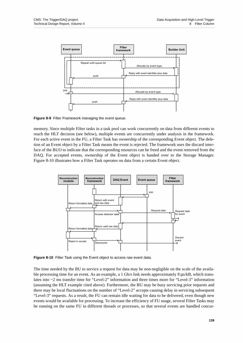
CMS: The Trigger/DAQ project Data Acquisition and High-Level TriggerTechnical Design Report, Volume II 8 Filter Column
memory. Since multiple Filter tasks in a task pool can work concurrently on data from different events toreach the HLT decision (see below), multiple events are concurrently under analysis in the framework.For each active event in the FU, a Filter Task has ownership of the corresponding Event object. The dele-tion of an Event object by a Filter Task means the event is rejected. The framework uses the discard inter-face of the BUO to indicate that the corresponding resources can be freed and the event removed from theDAQ. For accepted events, ownership of the Event object is handed over to the Storage Manager.Figure 8-10 illustrates how a Filter Task operates on data from a certain Event object.
The time needed by the BU to service a request for data may be non-negligible on the scale of the availa-ble processing time for an event. As an example, a 1 Gb/s link needs approximately 8 µs/kB, which trans-lates into ~2 ms transfer time for “Level-2” information and three times more for “Level-3” information(assuming the HLT example cited above). Furthermore, the BU may be busy servicing prior requests andthere may be local fluctuations on the number of “Level-2” accepts causing delay in servicing subsequent“Level-3” requests. As a result, the FU can remain idle waiting for data to be delivered, even though newevents would be available for processing. To increase the efficiency of FU usage, several Filter Tasks maybe running on the same FU in different threads or processes, so that several events are handled concur-
Figure 8-9 Filter Framework managing the event queue.
Figure 8-10 Filter Task using the Event object to access raw event data.
Builder UnitFilter
frameworkEvent queue
pop
Repeat untill queue full
push
push
Reply with event identifier plus data
Reply with event identifier plus data
Allocate by event type
Allocate by event type
Reconstructionmodule
Reconstructionframework DAQ Event Filter
frameworkEvent queue
pop
Return with eventand raw dataReturn formatted data
Return formatted dataReturn valid raw data
Desctructor
Request datafor event
Discardevent
Request data
Reject or accept
Access detector data
139

CMS: The Trigger/DAQ project Data Acquisition and High-Level TriggerTechnical Design Report, Volume II 8 Filter Column
rently and the CPU idle time is minimized. The actual number of concurrent tasks will depend upon prop-er optimization of the service and transfer time, and on the specific scheduling policy of the operatingsystem.
8.4.1.2 The Filter Task
The High-Level Trigger selection algorithms, described in detail in Chapter 15, "Physics Object Selectionand HLT Performance", run as plugins in the context of the Filter Task. The HLT application consists ofan event loop, a series of reconstruction units performing, on demand, parts of the reconstruction neces-sary to reach the trigger decision, and a number of filter modules that apply the selection criteria. The var-ious modules are integrated through the use of base software which is common to the offlinereconstruction [8-1]. Control messages and configurable parameters are dispatched to the application bythe local segment of the configuration and control system. For example, the filter application may bestarted, suspended or stopped by a message from the Subfarm Manager. Whenever a task is available, theframework assigns to it a new Event object for processing. The execution of the HLT application is direct-ed by a steering module. This steering code minimizes the amount of processing time by only running thefilter modules relevant for a given event type, or according to its Level-1 information. Following a policyset out in the configuration of the HLT, certain modules can break the processing and unconditionally re-ject the event (HLT veto). In all other cases, an event is accepted if it has been accepted by at least one ofthe relevant filter modules. An alternative option which is always available is to process an event until thefull chain of filter modules has reached a decision. This can be useful later in the offline processing stepwhich can utilize the result of the filter modules to classify the event as a candidate for different datastreams.
After an accept or reject, the filter application may perform additional calculations before dispatching theresponse to the framework. The HLT application is then ready for a new event, which means all interme-diate objects produced in the reconstruction have been deleted.
The HLT application accesses raw data in the form of buffer sequences containing data from several RUs.For each buffer, the framework handles the creation of a map of pointers in the Event object. When thefilter application attempts to access data from a specific part of the CMS detector, the map is searchedand, in case the data is missing, the framework issues the appropriate request for that data, and blockswhile waiting for the data to arrive. If the search is successful, or upon reception of data from the BU, apointer is returned to the beginning of the relevant portion of data, together with the size of that portion.The set of event fragments requested from the BU may include portions that have not yet been explicitlyaccessed, according to static or dynamic policies set out in the Filter Unit configuration.
The HLT application formats data fragments into objects. This may involve the invocation of methodsfrom detector geometry, condition and calibration classes etc. The data structures thus created are tran-sient and have the same life span as the event.
All intermediate information produced by the filter application during the processing of an event, can beattached along with raw event data to the Event object. Before an accepted event is handed to the storagemanager, it might be necessary to finalize its data content by collecting data that have not been requestedso far or have not been delivered. The request and formatting of these data is the task’s last operation onthe event.
The HLT application is dynamically loaded into the framework using a standard service method. Onceplugged in, the application waits for configuration and initialization and then goes into a paused state.Upon reception of a “start” message from the Subfarm Manager, it enters the event loop. Eventually, asuspend or stop message may be received. A suspend does not stop execution on the current event, but
140

CMS: The Trigger/DAQ project Data Acquisition and High-Level TriggerTechnical Design Report, Volume II 8 Filter Column
will block after the latter has been processed. A stop stops execution independently of the status of thecurrent event. Neither command clears the state of the reconstruction, for which an explicit reset messagemust be issued.
All configurable parameters, which must be controlled from outside the application, must implement aspecific ConfigurationElement interface to be published to the configuration and control services. Modifi-cations to configurable parameters will only take effect at event boundaries or “run” boundaries, depend-ing on the policy set out in the configuration for that specific parameter.
All the reconstruction and filtering parameters that need to be monitored by the online monitor consumersvia the SM, will have to implement a specific MonitorElement interface to be published to the Filter Mon-itor. The HLT application may include monitor components which perform specific reconstruction oranalysis used to monitor the application performance, producing complex results such as histograms. TheMonitorElement interface supports a publish and subscribe mechanism to give access to such complexdata types.
In order to allow for immediate notification of error conditions or other situations that need system-wideresponse or operator intervention, a special MonitorElement, called AlarmElement is always publishedand made available to every component of the Filter Unit, including the HLT application. Alarm messag-es posted to the AlarmElement are queued, so that no alarm message is cleared before having been noti-fied to all subscribed clients (and having been acknowledged by all subscribed clients, see below).
8.4.1.3 The Filter Monitor
The Filter Monitor serves several different purposes: it caches monitor information that has been previ-ously published to it by one of the Filter Unit components, keeps track of clients which subscribed for up-dates, and performs updates by delivering monitor information to the subscribers. It is also responsible fornotification of AlarmElement messages and for feeding the event display queue on the relevant clients.
Updates to monitor clients are performed by periodically waking up an update thread or process at inter-vals set out in the configuration. The update thread subsequently dispatches the data content of all Moni-torElements which varied since the last update to the relevant clients. Updates of MonitorElements do notneed to be acknowledged by the consumers.
Notification of alarms is preemptive: all the AlarmElement clients are notified as soon as the alarm isknown to the Filter Monitor, and reception has to be acknowledged before processing can continue. It ispossible, by issuing an appropriate command from Run Control, to mask certain types of alarms.
The Filter Monitor periodically notifies the subscribers of the special EventDisplay element with the fulldata content of the last event marked for display (according to the relevant configuration parameters).
The Filter Monitor interface allows a client to retrieve the full list of available MonitorElements, and toregister the client for update notifications (subscription). These interface extensions are implemented ac-cording to the principles and using the facilities described in Section 11.2.2. The Filter Monitor is capableof notifying any subscribed client which complies to the specification for control and monitoring commu-nication using the standard web protocol, as outlined in Section 11.2.5.
8.4.1.4 The Storage Manager
The Storage Manager takes ownership of events which have been accepted by the HLT, and are thereforemarked for storage. An accepted event consists of the entire set of detector raw data as delivered to the
141

CMS: The Trigger/DAQ project Data Acquisition and High-Level TriggerTechnical Design Report, Volume II 8 Filter Column
FU1, and of all the object collections that have been attached to it as a by-product of the HLT reconstruc-tion and selection. The event is then stored remotely on the Subfarm Manager using a specific interfaceand protocol. This protocol will match the one chosen for persistent storage of event data in the context ofthe offline framework. The actual implementation of the Storage Manager will therefore depend on thischoice [8-2]. After successful delivery of an event to the persistent services of the Subfarm Manager, theStorage Manager deletes the event, thereby triggering the issue of a discard message to the BU.
8.4.2 Internal Error Handling
In the event of an error condition in the HLT application, an exception is raised. The exception is caughtby the first element of the filter application which is able to handle it. In case the filter application is notable to recover from the error condition, the unhandled exception is passed on to the framework whichthen takes action by restarting the faulty task and reassigning or discarding the event(s) on which thefaulty task was working2. A recovered error condition (e.g. a task crash and subsequent restart) is loggedto the SM via the monitoring interface. A failure of one of the components, or the failure to recover froman error condition after a certain number of attempts, will cause the FU to transition to the failed state (seeSection 11.2.2 and Section 12.3.1, "State Definitions and System Synchronization"), and the failure willbe logged, if possible, to the SM. No error condition of the HLT application shall leave the FU in an unde-fined state.
Failure to transfer an event marked for storage to the persistent services of the SM (timeout) results in anexception being raised by the storage manager. Since the fault may be transient, an alarm is first issued tothe SM and the failed transaction is reiterated. After a certain number of attempts, a connection failure isassumed. Events in the queue are flushed and the FU transitions to a paused state, waiting for operator in-tervention.
8.5 Farm Control and Monitor
The configuration, setup and management of a large farm of computers, both from the hardware and oper-ating system point of view, is a common problem in large High Energy Physics experiments. In this re-spect, the Filter Farm, consisting of “Commercial Off the Shelf” (COTS) components, will, as far aspossible, adopt commercial hardware and software tools. These products, and possible home grown soft-ware if needed, must satisfy requirements which are common to online and offline farms, and to GRIDproduction centers [8-3]. Therefore, common solutions are expected to be adopted wherever possible.
This section is devoted to the requirements and constraints on Control and Monitor operations which arespecific to the Filter Farm. For each specific scenario, a sequence of operations is described, with empha-sis on operations that are critical for efficient data taking.
The Farm will be arranged, as previously stated, in a hierarchical structure consisting of a number ofsmaller, independent subfarms. Any configuration, control or monitor operation will, in general, follow atree structure, as exemplified in Figure 8-11.
1. Stripped of all DAQ-specific header and trailer information.
2. Depending on the type of failure, the event can be tagged as corrupt and not reassigned for processing. It will bepossible to store any event causing a failure condition in the filter application for further analysis.
142

CMS: The Trigger/DAQ project Data Acquisition and High-Level TriggerTechnical Design Report, Volume II 8 Filter Column
8.5.1 Subfarm Manager (SM)
The Subfarm Manager (SM) is the supervising element of a subfarm, representing it, to all external enti-ties, as a single element of the DAQ, which can be controlled and monitored in unison. It also representsthe subfarm’s access point to computing services.
The core of the SM is a generic application server, into which various services can be plugged to maintainthe configuration of the nodes in the subfarm, relay control messages coming from external entities suchas the RCMS, keep track of the state of each node, and collect, process and present monitor informationon behalf of external consumers.
Besides the software services mentioned above, the SM hardware hosts the mass storage systems wherethe reference copy of all the necessary software and external data structures (such as calibrations and con-stants) are resident. This includes the operating system, general purpose software libraries as well asHLT-specific libraries. This storage system must have a high level of redundancy. The SM machine alsoserves as the central boot node for all the subfarm machines. Finally, the SM hardware hosts the massstorage system for local data storage1. In this last function, it represents the point of access for data trans-fer to the central storage system and the offline production farms.
8.5.1.1 SM Functionality and Elements
A block scheme of the Subfarm Manager is shown in Figure 8-12. The various services are coordinated asplugins by the application server to provide a unique point of access for RCMS and monitor clients, andto give a uniform interface to the various functions of the subfarm. A Subfarm monitor handles the sub-scription and collection of monitor and alarm information from all the FU nodes. Monitor information isstored in a transient cache for local elaboration and distribution. A Monitor and Alarm engine can elabo-rate and analyse this information, as well as state information of FUs, SM and the local storage. Thresh-olds on various observables related to these components can be set here to produce alarms and warningsto be delivered to Run Control or other clients. Alarms originated by the FU or raised locally, can be
Figure 8-11 Filter Farm hierarchy structure and message flow. a) A Run Control command is distributed to allFU nodes. b) The Filter Farm Manager sends a command to a specific subfarm. c) A command is issued directlyto one of the FUs for debugging purposes. d) One of the FUs reports an alarm or updates a monitored parame-ter in the RCMS.
1. The controller machine for the local mass storage system may, for the sake of robustness, be physically separatedfrom the SM, although being logically part of it.
Sub-farm Manager (SM)
Farm Manager (FFM)
Run Control and Monitor (RCMS)
Filter Units (FU)
SMs
FFM
RCMS
FUs
SMs
FFM
RCMS
FUs
SMs
FFM
FUs
RCMS
Localdebugging
SMs
FFM
RCMS
FUs
a) b)
c) d)
143

CMS: The Trigger/DAQ project Data Acquisition and High-Level TriggerTechnical Design Report, Volume II 8 Filter Column
masked in the Monitor engine. Control and Configuration messages are distributed upon request fromRCMS by the corresponding service, and the State tracking service collects responses to monitor the re-al-time state of the system and acknowledge state transitions to the RCMS. The SM supervises the file-system containing the reference code, configuration data, and the replica of the Run Condition andCalibration Databases, through the Configuration manager, and monitors the state of the local mass stor-age on behalf of Run Control. To give uniform access to the Farm resources, the SM control and monitorinterfaces to the RCMS follow the DAQ “standard” and are identical to the corresponding interfaces ofthe FU.
The SM Presenter elaborates dynamic representations of the monitor and state information for browsingby external clients via the standard Web interface.
8.5.1.2 Error Handling
The Subfarm Manager collects information about the state of the FUs in the subfarm. The FUs update thisinformation with a frequency which is defined in the configuration. If a FU fails to communicate its statewithin a certain time period, it can be polled by the SM. In lack of response from a certain node, thenode’s state is set to failed in the SM. Depending on a policy set out in the configuration, the SM may ormay not try to restart the failed FU. The change in state of the subfarm is immediately communicated tothe Farm Manager. When the number of active nodes in a subfarm falls below a quorum set in the config-uration, the SM raises an alarm flag. In this event, some of the Builder Units may not be able to cope withthe full input rate, thus causing a performance deterioration of the whole DAQ. The Farm Manager canreconfigure the system, reassigning the relevant BUs to different Filter Units.
Thanks to the usage of asynchronous protocols for communication with the FUs, the coupling to the SMservices is sufficiently loose to guarantee that the subfarm may continue working in the event of a failureof one of the services, or of the whole server. On the other hand, such a failure will make it impossible tocontrol and track the state of subfarm nodes, or update run conditions or parameters. A backup systemwith Subfarm Manager functionality can be made available to take control in the event of an SM softwarefailure. SM hardware failures, on the other hand, affect the subfarm functionality because of the tight cou-
Figure 8-12 Subfarm Manager block scheme.
Subfarm Monitor
Configuration and code Manager
Control distribution
Application Server
Monitor cache
Monitor and alarm engine
FCN State tracking
Local storage manager
Presenter
(web interface)
DAQ interfaces
DSN
Code and Configuration
file system Local mass
storage CSN
Comp Services interface
144

CMS: The Trigger/DAQ project Data Acquisition and High-Level TriggerTechnical Design Report, Volume II 8 Filter Column
pling introduced by the local output storage. This case has been analysed in Section 8.4.2. See alsofootnote 1 of Section 8.5.
8.5.2 Farm Setup for Data-taking
When the RCMS initiates the setup sequence of the DAQ system to prepare for data taking, each of theFU nodes will create an instance of the FU framework. From then on, the state of the FU is controlled andknown at all times to the SM. Each SM, in turn, reports the status of all its nodes to the RCMS. When thefarm is configured, the HLT application is downloaded to the SMs. The SMs in turn serve the binary totheir nodes, which are subsequently requested to upload it to memory, including all relevant libraries.1
When the system is initialized, bootstrap information (e.g. geometry, run conditions, calibrations etc.) aredownloaded by the SMs from the appropriate servers and then distributed to the FU applications on re-quest. Each node keeps a private copy of this information. At the end of the initialization phase, when allFU nodes report being ready, the subfarm goes into ready state and the transition is reported to Run Con-trol, which may then start data taking.
The setup and control of the HLT tasks inside the individual FU nodes is the task of the Subfarm Managerunder the supervision of the RCMS. This includes the following:
• bootstrap of the reconstruction application
• control of the state of each of the HLT tasks
• HLT parameter setting
• upload of a trigger table
• Resetting of a task after an exception
• Notification of changes in the run condition and/or calibration db’s
• Error detection (and generation of alarms from limits)
• Monitoring of a task’s vital parameters (counters, accept rates, trigger and detector maps)
8.5.2.1 Upload of a New Trigger Table in the Filter Farm
The HLT tasks accept and discard events on the basis of a trigger table of relevant trigger channels, whichlists the physics objects and quantities, and the cuts to be applied to them. During a data taking period, thetrigger table is adjusted to account for variable luminosity, novel physics channels, detector malfunctions(e.g. dead channels, resolution deterioration) and other parameters. Furthermore, during a single machinefill, a broad variation of luminosity is possible and it may be necessary to switch from a high- to a low-lu-minosity trigger table while data are being taken. The loading of a new trigger table can be disruptive,since a certain amount of time is needed to update all the FU nodes. During this time, the system is in amixed state where a fraction of the FUs uses the old and a fraction the new trigger table.The change of thetrigger table must be unambiguously logged, so that during offline analysis it will be possible to associateeach event with the relevant trigger table. If the trigger table change requires processing to be temporarily
1. This may in practice mean: 1) the Farm Controller gets a copy of the new software from a file server. It then in-structs the Subfarm Managers to make a local copy (e.g. the relevant disk is nfs mounted by all SMs). 2) The SMs,when done, instruct all their nodes to get the files (e.g. the SM relevant disk is nfs mounted by all FUs in the sub-farm). If there has been no code update, the message only triggers a file read from the local disk on each Filter Unit.
145

CMS: The Trigger/DAQ project Data Acquisition and High-Level TriggerTechnical Design Report, Volume II 8 Filter Column
stopped on the subfarm, this interval has to be kept as short as possible in order to keep the DAQ efficien-cy high.
8.5.2.2 Handling of Run Conditions and Calibration Databases
The HLT tasks need information about run conditions (detector geometry, detector status, dead channels,alignment constants, beam characteristics etc.) and detector calibration constants. Some of these informa-tions may vary only seldom or not at all (such as the geometry) and can be accessed only once at startup,while others may vary on a relatively short time scale (e.g. fine beam alignment). Many of these informa-tions are cached locally on the FU at loading time. To reduce the load on the central information servers,only Subfarm Managers are allowed to download information centrally, and then redistribute it to their lo-cal nodes. Care must be taken to avoid mismatches between different subfarms, such that they use differ-ent calibration sets or different dead channel lists. However, it must be possible, after an event has left thefarm, to trace back all constants and conditions that were used to select it. The “standard” unique run andevent numbers will be a shorthand for a structure pointing to a certain combination of conditions and cal-ibrations constants.
8.5.3 Online Farm Monitoring
During data taking, it must be possible to monitor vital parameters of the filter farm from the individualnode level to the overall farm level. These parameters range from simple accept and reject rates to com-plex histograms of raw data or reconstructed quantities. For some of them, an aggregate view is sufficient,whereas for others, it is necessary to be able to collect information from a single subfarm or node. In somecases, a certain delay in data collection is acceptable (such as event displays, etc.), whereas other quanti-ties must be monitored in quasi-real-time. The collection of information by the monitor clients must notinterfere with normal running of the HLT tasks. Therefore, wherever possible, monitor data is collectedand elaborated by the SM on behalf of other consumers. When this is not possible, data are accumulatedby the Filter Units and delivered to consumers which must then elaborate them autonomously.
A possible, non exhaustive list of monitorable quantities is:
• Current run condition and calibration constants by node
• Current reconstruction parameters and trigger table by node
• Event latency distribution by node, where the event latency comprises the time the event is in theevent queue and the processing time
• Recoverable exception conditions detected by the reconstruction code
• Individual L1 accept rates by node, by subfarm, and aggregate
• Processing time distribution for events broken by event and trigger type
• Individual accept and reject rates of each selection algorithm and/or path in the HLT
• Detector maps for raw data, basic reconstructed objects, and HLT objects
• Instantaneous luminosity
• Beam position and beam parameters as seen by the tracker
• Characteristics (position, energy, momentum) of physics objects used by the HLT (e.g. mean Pt ofelectrons, photons and muons, mean total and missing transverse energy in jet events, reconstruct-ed mass of Z boson etc.)
146

CMS: The Trigger/DAQ project Data Acquisition and High-Level TriggerTechnical Design Report, Volume II 8 Filter Column
• Full representation of raw events and trigger objects sampling the whole farm.
8.5.4 Installation and Testing of HLT Code
8.5.4.1 HLT Coding Guidelines
The code that runs in the filter farm to perform HLT selection has to follow strict guidelines concerningthe usage of resources (network, memory, CPU time) and the handling of errors. It also has to undergostrict functionality tests prior to its actual deployment.
Any access to external resources by an HLT task results in a large number of operations in the overallfarm. No direct access to external resources, besides those defined by standard run condition and calibra-tion access interfaces, is thus allowed. The use of external software, which internally makes use of operat-ing system resources (e.g. network or shared resources) is restricted. As an example, the adoption oflibraries which covertly make use of shared memory or temporary disk files must be avoided.
The memory footprint must be under control at all times. A candidate filter module must be profiled formemory usage before being included in a test application. The CPU time usage under “normal” condi-tions, including the CPU usage distribution, must be specified and measured on “real data”.
All exceptions a module can raise must be declared in the module specifications, so that they can be han-dled properly.
Code to be included in a filter application must follow the standard CMS coding guidelines and qualitychecks [8-4] and is subject to a standard process control [8-5]. Additional requirements will be the subjectof a specific guideline document.
8.5.4.2 HLT Code Burn-in Sequence
Code for HLT undergoes the same versioning and release sequence as the offline code. A major version ofthe filter application will only include modules released with that major version. No new modules can beadded. Bug fixes to existing modules will increment the minor version number. When a new filter appli-cation is ready for release, it is first validated in an offline farm against a known dataset. If the offline val-idation is successful, the new filter application is tested in a special section of the filter farm.
Builder Units in the test partition are assigned a special event type called duplicated event. The EventManager tags random events to be duplicated, with a frequency defined in the configuration. A duplicatedevent is assigned once to a BU in the farm section running the production application, and then oncemore, to a BU in the test partition. Alternately, a single subfarm can be split into a production and a testsection, and the same events allocated by the BU to one FU in the production and one in the test section.Duplicated events then go into a special output stream. Validation is performed in the offline farms usingdata from the test and production streams.
147
CMS: The Trigger/DAQ project Data Acquisition and High-Level TriggerTechnical Design Report, Volume II 8 Filter Column
8.6 Prototypes and Results
8.6.1 Builder Unit Prototype
The BU prototype results were obtained running the software components included in the XDAQ data ac-quisition framework (see Chapter 11, "Cross-Platform DAQ Framework (XDAQ)"). The BU implementsthe interfaces described in Section 8.3.2.
A first setup consists of four PCs with a single 64bit/66MHz PCI bus and a Pentium III processor for theRU, a fifth PC running a BM, and an additional PC for the FU. A dual 64bit/66MHz PCI bus/dual CPUPC (Dell Poweredge 1550) was used for the BU. All machines run the Linux operating system and areconnected through a Myrinet 2000 network, accessed using the Myricom GM communication library1. Inthe setup, the RU acts as a data source for event fragments and the FU as data sink that continuously re-quests complete events. The FU request messages are gathered in groups of 256 and the RU deliversfixed-size fragments of 8 or 16 kB, so the total event size is 32 or 64 kB respectively. The resource poolfor event fragments in the BU is configured at 256. The throughput is sampled at the FU by measuring thetime needed to assemble 105 events. It is 194 MB/s and 204 MB/s respectively for 8 and 16 kB fragmentswhich satisfies the required throughput of 200 MB/s.
8.6.2 Filter Unit Prototypes
8.6.2.1 Tests of BU-FU Communication Protocol
The BU-FU communication protocol has been implemented for this test within the XDAQ data acquisi-tion software framework. The BUO feeds dummy event data to several FUs over a Gigabit-Ethernetswitching network using TCP/IP. Event data are segmented in chunks corresponding to a given HLT filterprocedure. Chunk average sizes correspond to current estimates of raw data sizes from the various detec-tors, and the actual size is extracted from a log-normal distribution to account for fluctuations. A paramet-ric Filter Task in the FU implements a step-wise filtering procedure where the average service time ofeach step, and the corresponding rejection factor, can be set to match a specific HLT configuration. Theservice time fluctuations are accounted for by extracting the actual times from a log-normal distribution.
The test shows that the BU-FU protocol is adequate. The BU can operate at an event rate of 200 Hz for anaverage event size of 1 MB, if the average HLT service times are set appropriately to match the input rate.The system reaches a steady state which depends only weakly on the level of fluctuations in the event siz-es and fragment times. As an example, for the two-step filtering described previously, a steady throughputof 66 MB/s is observed at the BU output, when the 10 FUs connected provide an average total servicetime of 50 ms/event. This is achieved by setting the average “Level-2” service time at 40 ms with a rejec-tion factor of 100. The subsequent “Level-3” step can then be performed in an average of up to 250 ms.
8.6.2.2 Prototype HLT Application
To demonstrate the feasibility of operating an offline reconstruction procedure in the context of the FilterUnit, the integration of the CMS reconstruction software framework (COBRA [8-1]), and of the CMS ob-
1. For an overview of Myrinet network products and related protocols see Appendix A.2, "Myrinet Technology andProducts"
148

CMS: The Trigger/DAQ project Data Acquisition and High-Level TriggerTechnical Design Report, Volume II 8 Filter Column
ject oriented reconstruction (ORCA [8-6]) in the Filter Unit prototype has been carried out. The raw-dataaccess interface (Event object data bus) and the DAQ-specific event loop structure are implemented asextensions to the offline framework. Raw event data in an arbitrary format is read in by a standaloneBUO, transferred over the network using the protocol described above, and accessed by a generic ORCAreconstruction module. To achieve this, a skeleton implementation of the raw detector data formattingwas also prototyped as a replacement library for ORCA. The prototype HLT application was successfullyoperated and controlled in a Filter Task through the Filter Unit framework. Final design and implementa-tion of configuration and monitor layers, as extensions to the offline framework, is ongoing.
8.6.2.3 Prototype Reconstruction Code for HLT
The details of the current reconstruction software framework used by the HLT algorithms can be found inChapter 15, "Physics Object Selection and HLT Performance". For the purpose of this chapter, two keymeasurements are worth mentioning, namely that the current software requires approximately 150 MB ofmemory and roughly 400 ms/event passing the Level-1 Trigger requirements described in Chapter 14,"Detector Simulation and Reconstruction".
8.6.3 Subfarm Manager as Control and Monitor Server
A Subfarm Manager prototype software, based on the Apache Tomcat servlet container [8-7] has beendemonstrated in a small scale setup. It integrates the online software prototype services described inSection 11.2.7, "Configuration, Control and Monitoring Components", and is able to distribute configura-tion and control messages using the SOAP protocol. State tracking and monitor information collection areimplemented as servlets, and the server is able to present dynamic information about the system to astandard browser. Among the future activities, larger scale tests of configuration and command distribu-tion will be performed. A complete implementation, which will also take into account surveys of availa-ble products and work on analogous components for the Run Control System, will be completed for usein the subfarm test-bench (see Section 8.7.3).
8.7 Technology Outlook and Schedule
As mentioned numerous times throughout this Technical Design Report, the design of the CMS DAQ isbased on the use of Commercial Off-The-Shelf solutions (COTS) to the greatest possible extent. Whatev-er CMS-specific hardware has to be developed, it is usually placed close to the detector, where theLHC-specific or the CMS-specific requirements are such that COTS systems can either not be procured atall, or can be procured but at relatively high cost. The elements of the Filter Column, however, are themost clear case where commercially available hardware can satisfy the requirements. An implementationof the subfarm via a number of standard Personal Computers (PCs), possibly with dual CPUs, and a 12-24port Gigabit Ethernet switch acting as the FDN is going to be both inexpensive and easily maintainable,given the wide availability of these elements. This is especially true when one considers the year 2006 asthe actual time scale when much of the DAQ hardware will be procured.
The actual design of the Filter Column can accommodate essentially any technology for the intelligencesinvolved (i.e. the BU and the FU) along with any technology for the switched interconnect. The actualchoice of BU will be influenced by the technology chosen for the Builder Data Network that connects theBUs to the Readout Units: BU hardware will have to be compatible with the associated Network InterfaceCards of this network. Nevertheless, given the observed explosion of industrial offerings in this general
149

CMS: The Trigger/DAQ project Data Acquisition and High-Level TriggerTechnical Design Report, Volume II 8 Filter Column
area, the Filter Column components can easily profit, with minimal disturbance, of most of the announcedtechnological improvements.
8.7.1 Hardware
8.7.1.1 Builder Unit
The basic implementation of the BU is a PC with two independent 64-bit/66 MHz PCI busses and 1GBmemory. The CPU is not an issue given that the BU does not process the event data, but only assemblesthe fragments into full events.
It should be pointed out that the BUs in the CMS DAQ are not expected to be all identical machines. Asexplained in Part 1, the CMS DAQ will be installed in a number of steps that will be timed to facilitate theoperation of the experiment, given the accelerator conditions and the financial resources available. Themost likely scenario is therefore one in which the RU Builders are procured at different times. Given theplanned BU implementation, it is clear that procurements separated in time by periods of ~6 months to ayear will result in different hardware being installed as BUs. With the current design and planned imple-mentation there is, a priori, no anticipated effect from this.
8.7.1.2 Filter Data Network Technology
The strategy for deciding on a FDN technology is analogous to that for deciding a BU implementation. Astandard commercial switched network can satisfy all requirements. As such, the most widely availableand possibly widely deployed network technology at the time of the procurements of the Filter subfarmswill be chosen. Already, as this TDR is being written, Gigabit Ethernet technology is within reach, interms of financial resources, for such a wide deployment. It is anticipated that by 2006-2007, the associat-ed costs will have dropped even further. Should Ethernet, in the next few years, become an obsolete tech-nology, the FDN will clearly utilize the new technology of choice. In brief, the system design is veryflexible, and it allows the use of any FDN technology.
8.7.1.3 Filter Unit Processors
The Filter Units, and in general the filter farm, will require a large number of inexpensive PCs. A poten-tial exception to this is the hardware for the Subfarm Manager, where a larger CPU server may be moreappropriate, or even necessary, given that the SM has to also serve as the basic source of code and config-uration data for the FUs in the farm.
8.7.2 Software
8.7.2.1 Operating System
With very large numbers of processors installed, the costs of a commercial OS can be significant. The ad-vent of Linux, with its high reliability and wide deployment in High Energy Physics, as well as its stand-ard UNIX interfaces to networking, has provided a “natural” solution for the Operating System, at leastfor the Builder Units and the Filter Units. At this point in time all indications are that the development andfurther deployment of Linux will continue in the relevant time scales.
150

CMS: The Trigger/DAQ project Data Acquisition and High-Level TriggerTechnical Design Report, Volume II 8 Filter Column
8.7.2.2 Other Software Components
All basic external software packages used in the current prototypes are either commercial or constitutepart of the Open Source software initiative. All technologies utilized, e.g. XML, SOAP, TCP/IP are stand-ard and widely available. Thanks to the layered architecture of the Online software, with middlewarescreening applications from lower-level core functions, an easy migration to new standards is anticipated.
8.7.3 Subfarm Test-bench
To continue verifying on a larger scale the architecture and design of the farm and related software, andtaking into account the general principles stated above, a test-bench composed of current COTS comput-ers and networks, with the level of complexity expected for a subfarm, will be assembled. This systemwill first of all provide the testing ground to verify the scaling properties of some of the configuration,control and monitor features described throughout this chapter. It will also be used to evaluate candidateproducts and technologies for hardware and system management, concentrating on specific aspects of anonline environment. Finally, it will be exploited for stress tests of reconstruction software, using simulat-ed event data with realistic formats, as they are being finalized by the detector groups. Ultimately, it willbe part of a complete, scaled down acquisition system which will implement the full chain of the DAQ.The test-bench will represent an intermediate step for validation of all the software components to be sub-sequently deployed in the CMS Filter Farm.
8.8 Summary
In this chapter the functionality and the design of the Builder Unit and the Filter Farm are described. Theevents which are assembled in the BU are processed in the Filter Farm in order to reach the HLT decision.This can be done in multiple steps to reduce the data traffic between the BUs and the Filter Units.
The Filter Farm is divided into independent subfarms in order to ease configuration, control, and monitor-ing of the large number of Filter Units. This modular concept results in a scalable system and improvesthe reliability against failure of single nodes.
In a BU protoype the required data throughput of 200 MB/s has been achieved. The interface between theBU and the Filter subfarm has been implemented in another prototype and the developed protocols havebeen successfully tested. A test-bench will be built to further analyse different software implementationsof the Filter Column components, to evaluate system management tools, and for performance measure-ments of reconstruction and selection algorithms.
8.9 References
8-1 V. Innocente, L. Silvestris and D. Stickland, on behalf of the CMS collaboration, “CMS Software Architecture. Software framework, services and persistency in High-Level trigger, reconstruction and analysis”, Comput. Phys. Commun., 140 (2001) 31;Coherent Object Base for Reconstruction, Analysis and simulation (COBRA), see http://cobra.web.cern.ch/cobra/
8-2 “Report of the LHC Computing Grid Project: Persistency Management RTAG”, CERN-LCG-2002-006, 5 April 2002.
151

CMS: The Trigger/DAQ project Data Acquisition and High-Level TriggerTechnical Design Report, Volume II 8 Filter Column
8-3 “DataGrid Work Package 4: Fabric Management, Report on Current Technology”, DataGrid-04-D4.1, 18 May 2001; The DataGrid Project , see http://eu-datagrid.web.cern.ch/eu-datagrid
8-4 J. P. Wellisch for the CMS software group, “The CMS Coding and Design Guidelines”, CMS Note 1998/070.
8-5 The ISO/IEC Joint Technical Committee 1 (JTC1), Subcommittee 7 (SC7) Working Group 10 (WG10), Terry Rout (ed.), ISO/IEC DTR 15504 Software Process Assessment;“Report of the LHC Computing Grid Project: Software Management Process RTAG”, CERN-LCG-2002-009, 6 May 2002.
8-6 ORCA, Object-oriented Reconstruction for CMS Analysis, see http://cmsdoc.cern.ch/orca/
8-7 The Jakarta Project: Apache Tomcat v. 4.0; http://jakarta.apache.org/tomcat/index.html
152

CMS: The Trigger/DAQ project Data Acquisition and High-Level TriggerTechnical Design Report, Volume II 9 Event Builder Fault Tolerance
9 Event Builder Fault Tolerance
Important elements of the DAQ system are the error-handling procedures and other mechanisms that al-low it to operate with a sufficiently high efficiency. This chapter discusses various aspects of redundancyand fault tolerance of the DAQ architecture and design. It is aiming to demonstrate that the two are ex-pected to lead to a system that can deliver high-quality data with high efficiency.
Dependability is defined as the probability to accept and assemble the next event. A high operation effi-ciency and dependability is the result of three conditions:
• rarity of cases at which the system has to stop its operation,
• quick identification and equivalently fast recovery procedures for those error conditions that affectthe quality of the data in a significant way,
• tolerating and possibly ignoring error conditions that have only a minor effect on the data quality.
The key element to achieving the above three elements is the correct categorization of failures in the sys-tem. The purpose of this analysis is thus to determine the failures that should be avoided, the ones thatshould be tolerated and the ones that can be ignored. This categorization depends on the mean time be-tween failures, the down time required to recover from the resulting errors as well as the cost of toleratingor avoiding them. Clearly, very rare failures that happen once a year can be ignored, if the system can beup and running again within about an hour with a simple system reset.
On the other hand, a more frequent transient fault [9-1] needs special attention. A fault is transient if it ex-ists for only a short amount of time and disappears without an explicit recovery procedure. A transientfault might lead the system into an incoherent state which can be permanent. If this state is not detectedand handled properly, it can eventually lead to a system failure which will, in turn, degrade the system’sdependability and reliability1. A system with the ability to recover from inconsistent states caused bytransient faults without outside intervention and regardless of the origin of the fault origin, is said to be aself-stabilizing system [9-2].
The plan to achieve a fault-tolerant design for the DAQ has been the following:
1. Catalogue an extensive list of possible faults together with their effects on the system, as well aspossible detection and recovery methods.
2. Supplement the CMS-DAQ system design in places that have been identified as potential sourcesof faults, by adding additional functionality or improved components.
3. Establish that the newly supplemented design is fault-tolerant by demonstrating that in the result-ing system all transient faults are handled in real-time and that, after relatively short periods oftime, the system resumes its correct operation.
4. Test the correctness of the actual implementation of the established fault-tolerant protocols by in-jecting faults to prototype software and hardware developed in the context of the CMS-DAQR&D.
Before giving the extensive list of possible failures and their detection and recovery methods for eachsub-system, it should be noted that, there is no single point of failure in the DAQ system which wouldbring down the entire system until it is repaired. The proposed system, with its modular design consisting
1. Definition: The probability that a system will perform its specified function, without failure under stated environ-mental conditions, over a required lifetime.
153

CMS: The Trigger/DAQ project Data Acquisition and High-Level TriggerTechnical Design Report, Volume II 9 Event Builder Fault Tolerance
of independent RU Builders1, will continue to operate, albeit with less performance, after identifying andisolating the faulty component. If one RU Builder fails the system will continue to build and filter eventswith the remaining RU Builders after re-configuration of the FED Builders2. If a FED Builder fails, thesystem will also continue to build and filter events from other parts of the detector, again after reconfigu-ration of the RU Builders. The only single point of failure prohibiting further operation is the FED Build-er for the Level-1 Trigger (see Section 4.2.5, "Data Flow in the FED Builder"),
The list of faults identified in the DAQ architecture and event building protocols is discussed inSection 9.2, "Error Analysis for the Event Building Protocol" along with the detection methods and theassociated reaction to the faults.
9.1 Fault Tolerance Requirements and Design Choices of the DAQ System
This section lists the design choices and suggested fault-tolerance requirements of the DAQ system anddiscusses the underlying reasons for these choices. Some of the items listed below are more of a designchoice than a requirement. The main motivation behind these choices is to maximize system availability.When the Event Building networks are fully loaded, any attempt to recover corrupted event data will de-crease system availability such that the product of the system availability and the system reliability at beststays constant. As long as the mean time between failures is large, the number of events sacrificed due toerror recovery will be acceptable.
1. All error states in the DAQ system shall be detected, logged and of the system shall be broughtback to a consistent state.
2. Sub-systems shall have self-stabilizing behavior for all external faults.
3. Sub-systems shall tolerate transient faults.
4. All data corruptions shall be detected and logged.
5. Application processes shall not assume that the inter-process communications are reliable.
6. Sub-systems shall be capable of performing forward-error-recovery (go to a state to that the systemwould have gone to if the error had not occurred).
7. Sub-systems are allowed to execute exception-handling methods which corrupt event data of a lim-ited number of events in order to maintain system availability.
8. Sub-systems could perform backward-error-recovery, however only if the system availabilitywould not decrease.
9. Sub-systems could implement fault masking3, provided this does not decrease system availability.
10. The system shall continue to operate with reduced performance in the presence of faulty compo-nents.
11. All persistent failures (e.g. a node crash) shall be detected and reported to the Problem Solver.
12. The system shall be reconfigurable in order to mask faulty components.
1. See Section 4.3, "RU Builder" and Section 4.4, "Partitioning".
2. See Section 4.2, "FED Builder".3. Fault masking allows the subs-system to ignore specified faults.
154

CMS: The Trigger/DAQ project Data Acquisition and High-Level TriggerTechnical Design Report, Volume II 9 Event Builder Fault Tolerance
13. Sub-systems shall provide monitoring and diagnostics services to facilitate the localization offaults.
14. Sub-systems shall monitor their resources and report any shortages to the Error Manager.
15. The event number should not be reset before O(1000) triggers1 since the last reset to avoid havingtwo events with the same event number in the Readout Unit Input module.
9.2 Error Analysis for the Event Building Protocol
This section gives a general description of the failure detection and exception-handling methods whichwill be implemented by functional units of the DAQ system. A detailed list of all failures that are handledby a unit, the details of their detection, and exception-handling procedures are described in the followingsub-sections. Supplementary information is given in Appendix E, "Fault Tolerance of Distributed Sys-tems".
Each node could produce a faulty message as a result of input failure and/or internal faults. For each mes-sage there are three possible faults, namely the loss of the message, a spurious message and the corruptionof some information contained in the message. Each node in the system shall implement the followingfault-tolerance behavior to handle input failures:
• A spurious message can be detected by comparing the message context either with the informationstored in the receiver if the message is a response to a request, or to information it expects. For ex-ample, a event number received by the Readout Units from the Readout Manager must increase byN (or have a reset value), where N is the number of RU Builders in the system.
• All messages shall contain sufficient information to allow identification of spurious messages.Standard encoding techniques will be used to ensure that a value error in these fields will not causea false detection of spurious messages. All detected spurious messages will be dropped by the re-ceivers, thus they will not change the internal states of these receivers.
• Similarly, any message with a detected-value error can be safely dropped at a receiver. Thus, theyappear to a receiver as omission failures. Well known techniques such as CRC checks will be usedto detect corruptions during transmission. Whenever possible, reliable communication protocolswill be used to recover from value-errors incurred during transmission (see Section 6.6.3, "Relia-ble Broadcast Protocol for the RCN"). It is noted that some of the messages with undetected value-error will be identified as spurious messages. Undetected spurious messages will have the same ef-fect as an undetected value-errors.
• Omission failures will be detected by “watchdog timers” or local sequence numbers. Whenever awatchdog timer expires, the node will perform a forward recovery and release all its resources allo-cated to the event in question. All messages arriving late (after a watchdog timer expires for a giv-en transaction) will be treated as spurious messages and will be dropped. In order to avoid falsedetection of omission failures, watchdog timer expiration will be long enough to cover most trans-mission delays.
Transactions with undetected value-error can not be differentiated from error-free transactions. Therefore,a node which receives a message with undetected value-error will not deviate from its standard behavior.However, it could generate omission failures, and spurious or corrupted messages.
1. Actual number of triggers between reset will depend on the concurrent events being build in the RUI which dependon the memory available for this purpose on the final system.
155

CMS: The Trigger/DAQ project Data Acquisition and High-Level TriggerTechnical Design Report, Volume II 9 Event Builder Fault Tolerance
9.2.1 Failure Modes of the Front-End System
Front-End Systems provide data fragments from various detector elements to the DAQ system for eventassembly. As with any node in the DAQ system, front-end nodes can also fail and produce omission fail-ures, spurious or corrupted messages. Value-errors in the detector data have no effect on the correct oper-ation of the DAQ system. Of course, in this case, the assembled event will contain the erroneous data.
Data from different detector elements belonging to the same bunch-crossing will be identified by twonumbers, a event number and a bunch-crossing number. These event numbers will be generated bycounters in the Front-End Systems from a common clock signal distributed by the Trigger and Timingsystem (see Chapter 5.2.1, "Trigger Timing and Control (TTC) System"). The event number incrementscontinuously with each Level-1 accept and counts the number of triggers since the last resynch. It wrapsaround after about 1 million triggers. The bunch-crossing number is generated by a 40 MHz clock andgives the bunch-crossing of an accepted trigger. It is resetted every orbit. Since the DAQ system uses thispair of numbers (or an alias of them) to assemble the event, any value-error in these numbers leads to anassembly of data from different triggers1.
A transient fault that causes the event number counter to over- or under-count (a value-error) does notstop the DAQ system. However, all assembled-events will be corrupted until the faulty counter is reset.This failure will be detected by the observation of data fragments with the same event number, but havinga different bunch-crossing number. On the other hand, over- or under-counting of the bunch-crossingnumber does not lead to a faulty assembly of events. However, such events can not be distinguished fromevents assembled from data fragments with value-error in their event numbers.
In principle, over-counting or under-counting failures of the event or bunch-crossing numbers could bedetected by the BU nodes, by checking the consistency of the numbers in an assembled event. In contrastto other transient failures which lead to event corruption at a small number of BU nodes, these failures aresingle-point failures which affect all BU nodes. Since their errors persist until a reset of the faultycounters, the late detection (in the order of seconds) of this class of failures results in the loss of a poten-tially large number of events. This may not be acceptable. The earliest nodes in the assembly chain whichcould detect these failures are the Readout Unit Inputs (see Section 9.2.2.2, "Readout Unit Input" for dis-cussion on how this error can be detected.).
9.2.2 Fault Tolerance of the Event Building Nodes
The event building protocol described in Section 5.3, "Event Builder Protocols and Data Flow" togetherwith the fault tolerance extensions summarized in the introduction of this section guarantees the end ofthe life cycle is reached for each event, even in the presence of transient faults. For all events in the sys-tem at a given time, if all nodes complete their activity and release all resources used in the event buildingprocess, then the DAQ system will be in a consistent state and ready to accept new triggers. In the processof recovering system consistency, intentionally or unintentionally, events being assembled could get cor-rupted. Since transient faults disappear from the system without requiring any intervention, an assemblyof events entering the system at a later time will proceed according to standard system behavior.
1. In principle, the event number alone will be sufficient to assemble events when there are no failures. Theevent/bunch-crossing number pair will facilitate the detection of certain failures.
156

CMS: The Trigger/DAQ project Data Acquisition and High-Level TriggerTechnical Design Report, Volume II 9 Event Builder Fault Tolerance
9.2.2.1 Front-end Readout Link
The “single input” Front-end Readout Link (FRL) boards with their associated Network-Interface Cards(NIC), behave as FIFO buffers and therefore do not deviate from their standard behavior with the occur-rence of input failures. All input failures will be transmitted to the output without any permanent effect onthe internal states of these nodes.
Due to the FIFO behavior of the readout, all input failures can be detected by comparing the eventnumber of the event data with an internal sequence counter local to the FRL. Although this simple mech-anism is sufficient to detect failures, it is not possible to localize the fault and invoke the proper recoveryaction. For example, the event number of the incoming event data will be different from the local FRL se-quence number if either the event number or the local sequence number has a value error.
Since the routing of the event data depends on the event number, any value error of this field, either at theinput of the FRL or generated due to an internal fault, can lead to miss-routing of the data fragment. Miss-routed data fragments will produce an omission failure for the intended destination node and spuriousdata for the node which will eventually receive it.
When a FRL merges two inputs, an omission failure at one of the inputs would lead to merging of datafrom different triggers. Although this error can be detected by comparing the event numbers from both in-puts and a local sequence counter, the loss of synchronization persists until the resynch of the front-endnodes. Miss-routing of the data will be avoided by the use of majority logic, however in this case, the as-sembled fragment might contain data from two different triggers and therefore it will be marked as cor-rupted.
9.2.2.2 Readout Unit Input
The Readout Unit Input (RUI) module will assemble data fragments from multiple (typically 8) FRLs andpresent the super-fragment to a Readout Unit (RU), preserving the trigger time ordering. All omissionfailures will be detected with a watch-dog timer and the event in question will be flagged as incompleteand passed to the RU, and the resources allocated to it will be released.
The RUI implements a credit scheme based traffic shaping to avoid data loss due to memory shortages.Nevertheless, it may run out of memory if the RUI fails to transfer super-fragments to the RU memory. Inthis case, the RUI will delete the oldest super-fragment(s) in its memory to make room for fragments fromnew triggers. This behavior will result in an omission failure at the RU input.
It is possible to detect most spurious messages by comparing the event number and the expected sequencenumber. Undetected spurious messages will corrupt the fragment being built with the same event number.However, this corruption can be detected by the RU, Builder Unit and /or Filter Unit by checking the con-sistency of the event data. When valid data for an event from the same FRL which corrupted the event inquestion by generating a spurious message arrives, it will be detected as a spurious message and will bedropped with no side effects.
By comparing the bunch crossing numbers of fragments from different FRLs, the RUI is in principle thefirst node which could detect data miss-alignment errors. If the error is a transient error, simply markingthe super-fragment as corrupted would be sufficient and no further action is necessary. However, if the er-ror persist the system has to be resynched (see Section 5.2.2.2, "Synchronisation Recovery").
157

CMS: The Trigger/DAQ project Data Acquisition and High-Level TriggerTechnical Design Report, Volume II 9 Event Builder Fault Tolerance
9.2.2.3 Event Manager
From the fault tolerance point of view, Event Manager (EVM) nodes maintain the state of Event-IDs theymanage and allocate them to BUs for event assembly. Each Event-ID has three states: “Free”, “Open” and“Allocated”. Receiving a trigger message from the GTP in the EVM causes one of the “Free” Event-ID’sto change its state to “Open”. The EVM informs the RUs that a trigger arrived and the event data was as-signed an Event-ID. Upon receiving an Allocate message from a Builder Unit (BU), one of the “Open”Event-ID’s will be assigned to the BU requesting an event for assembly and the state of the Event-ID ischanged to “Allocated”. A Clear message is always associated with a given Event-ID and its arrival willtrigger the release of an Event-ID. The Clear message changes the state of the Event-ID it is associatedwith to “Free”, thus making it available for reuse by future triggers.
An omission failure of the trigger message has no effect on the internal state of the EVM. However, sinceno readout command is sent to the RUs, event data associated with this trigger stays in the RU memory. Inthis failure mode, since all RU’s miss a readout command, no data corruption occurs for the proceedingtriggers. Again, the omission of the Allocate message has no effect on the EVM but generates an omis-sion failure for the expected Confirm message.
Since Clear messages are always associated with a given Event-ID, their omission will cause an Event-IDto remain ”Allocated” until the EVM watchdog expires. If the total number of Event-IDs in the system issufficiently large1, the watch-dog timers for each Event-ID can be replaced by a periodic but less frequentgarbage collection which checks the state of all Event-IDs.
In addition to the input failures mentioned above, an internal failure might trigger an unwanted statechange of an Event-ID. Below (see Table 9-1) is the list of all possible faulty transitions and the resultingfailure modes of the system.
Figure 9-1 State chart of an Event-ID.
1. The total number of Event-IDs in the system depends on the available memory in the RUs and BUs.
FreeEntry/Release EventID
AllocatedEntry/Allocated to BUID,
Confirm (EventID)
OpenEntry/Assign Event ID,
ReadoutAndClear(EventID)
After: [Expired] Clear [BUID = EventID allocated to BUID]
New Trigger [Top of the Free EventID queue]
Allocate [Top of the Open EventID queue]
158

CMS: The Trigger/DAQ project Data Acquisition and High-Level TriggerTechnical Design Report, Volume II 9 Event Builder Fault Tolerance
Table 9-1 List of all possible faulty transitions and the resulting failure modes of the system due to inter-nal EVM failures.
Faulty transition Failure modes
“Free” Event-ID is changed to “Open” Previous event which was associated with the Event-IDwill be reassembled. After successful completion of theassembly, Event-ID state will be restored to its correctstate and the system returned to its standard behavior.
“Free” Event-ID is changed to “Allocated” Event-ID and the associated resources stay blocked un-til the next garbage collection. No event is lost.
“Open” Event-ID is changed to “Allocated” The event associated with this Event-ID never gets as-sembled. The next garbage collection will release theEvent-ID for reuse.
“Open” Event-ID is changed to “Free”. The event in the RUs will be over written by a newevent and the original event will be lost.
“Allocated” Event-ID is changed to “Free” The Clear message expected in association with thisEvent-ID will be identified as a spurious message andwill be dropped.
If this Event-ID is used by a new trigger and a Clear-and-Readout command is executed before the eventpreviously assigned to this Event-ID gets assembled,the resulting over writing of the event fragments in theRU memories will corrupt the previous event.
“Allocated” Event-ID is changed to “Open” Same event will be reassigned for assembly and selec-tion.
The Clear message from the first assembly will getidentified as spurious and will be ignored.
Completion of the second assembly will free the Event-ID.
If the event is selected for archiving, the archive mighthave two copies of the same event if it does not catchthis failure.
159

CMS: The Trigger/DAQ project Data Acquisition and High-Level TriggerTechnical Design Report, Volume II 9 Event Builder Fault Tolerance
9.2.2.4 Readout Unit
A Readout Unit (RU) stores the event fragments received from its Readout Unit Input (RUI) node andprovides random access to the event data during event assembly. A RU receives a “Clear-and-Readout”command from the Event Manager (EVM) and “Send” messages from the Builder Units which it repliesto with “Cache” messages.
Due to the FIFO nature of the readout and the one-to-one relation between the incoming event fragmentsand the “Clear-and-Readout” messages, any loss of alignment between the command and the data, if notdetected and corrected, results in assembling of event fragments from different events. The loss of align-ment will be detected by comparing the event and bunch-crossing numbers in the command and data mes-sages.
Upon receiving the “Clear-and-Readout” command, a RU releases all resources used by the previousevent which was assigned the same Event-ID. The new event data are stored with this Event-ID only ifthe command and the data are aligned. Although this will prevent the assembling of fragments from dif-ferent events, all events will have missing fragments from faulty RUs until the alignment is re-estab-lished.
Realignment of the command and the event fragment can be established by removing the data and/orcommands from their respective input queues. This recovery will result in the loss of a few events, butwill be more efficient than a full system resynch. Table 9-2 lists various failure which upset the commandand data alignment along with the side effects of recovery.
Under normal operations, the number of event fragments stored in the memory of a single RU is equal tothe number of Event-IDs. Each RU will have sufficient memory to hold all fragments. However, internalfaults might lock some of this memory. A garbage collection will periodically reclaim the locked memo-ry. In principle, the asynchronous Trigger-Throttling System (see Section 5.2, "Trigger-Throttling System(TTS)") will prevent a RU memory overflow. If the throttle system fails, memory is freed by removingthe oldest event fragment from the RU memory.
BUs request a given event fragment using a “Send” message. The readout and transfer of the event frag-ment from the RU memory is not a destructive process and does not change the internal state of the RU.Therefore, an omission failure, a value error or a spurious message do not have any adverse effects on thestate of the RU. However these failures will propagate as RU failures.
1. A “Send” omission will result in an omission of the corresponding “Cache” message.
2. A spurious “Send” message from a BU will be replied with a spurious “Cache” message.
3. A value error in the destination field of the “Send” message will result in sending the event frag-ment to a different BU.
4. A value error in the Event-ID field of the “Send” message will generate a spurious “Cache” mes-sage containing the wrong event fragment.
5. A value error in the resourceID field of the “Send” message will be copied to the “Cache” messagewhich will be identified as a spurious “Cache” message in the BU.
In addition, due to internal errors, a RU can send the wrong event fragment. This failure can be detectedby checking the consistency of the event and bunch-crossing numbers of the request and the reply at theBU.
160

CMS: The Trigger/DAQ project Data Acquisition and High-Level TriggerTechnical Design Report, Volume II 9 Event Builder Fault Tolerance
9.2.2.5 Builder Unit
Following the Readout Unit event builder protocol described in Section 5.3, "Event Builder Protocols andData Flow", a Builder Unit (BU) node sends “Allocate” and “Clear” messages to the EVM and “Send”messages to the RUs. It receives a “Confirm” message from the EVM and “Cache” messages from theRUs as reply to an earlier “Allocate” and “Send” messages.
Table 9-2 Various failures that upset the command and data alignment along with the side effects ofrecovery.
Failure Side effect Recovery
Omission of a Clear-and-Read-out command
Input data queue has an addition-al event fragment.
Readout command aligns withthe next event fragment in the in-put data queue.
Remove the event fragment fromthe input data queue.
Omission of an event fragment Input command queue has an ad-ditional command.
Event fragment aligns with thenext command in the input com-mand queue.
Remove command from the in-put queue.
Spurious Clear-and-Readout command
Input command queue has addi-tional command.
Event fragment aligns with thenext command in the input com-mand queue.
Remove command from the in-put command queue.
Spurious event fragment from RUI
Input data queue has an extraevent fragment.
Command aligns with the nextevent fragment in the input dataqueue.
Remove event fragment from theinput data queue.
Value error in the Event number field of the event fragment.
Next Command aligns with thenext event fragment in the inputdata queue
Remove both event fragment andcommand from the input queues.
Value error in the bunch-crossing number field of the event frag-ment
Next Command aligns with thenext event fragment in the inputdata queue.
Remove both event fragment andcommand from the input queues.
Value error in the Event number field of the Clear-and-Readout command.
Next Command aligns with thenext event fragment in the inputdata queue.
Remove both event fragment andcommand from the input queues.
Value error in the bunch-crossing number field of the Clear-and-Readout command.
Next Command aligns with thenext event fragment in the inputdata queue.
Remove both event fragment andcommand from the input queues.
161

CMS: The Trigger/DAQ project Data Acquisition and High-Level TriggerTechnical Design Report, Volume II 9 Event Builder Fault Tolerance
Omission failures of “Confirm” and “Cache” messages will lock the resources allocated to the event inquestion. However, proper use of watch-dog timers will detect these resource dead locks and resolvethem. Partially assembled events will be passed to Filter Units (FU) as incomplete events. Omission fail-ure of a “Confirm” message also triggers an omission of the associated “Clear” message at the EVMwhich locks the Event-ID in question permanently if not detected and handled by the EVM.
A value error of the Event-ID field will not effect the event building functions. However, depending onthe actual state of the Event-ID, a BU might assemble and later release an event assigned to another BU,or assemble an event incorrectly if there is an ongoing readout for this Event-ID. In the first case, one ofthe two “Clear” messages which is generated at a later time will appear as a spurious message to theEVM. The latter case will be identified by consistency checks of the assembled event at the FU or BU.
9.2.3 Fault Tolerance Analysis of Filter Unit - Builder Unit Communication
Filter Unit (FU) - Builder Unit (BU) communication is based on Allocate, Collect, Discard and Take mes-sages as described in Section 8.3.2, "Data Flow". Table 9-3 lists errors that may occur in the BU-FU com-munication.
9.3 Persistent Failures
The chosen exception handling mechanism described above is based on the assumption that the fault istransient and external to the node which detects the resulting failure. Therefore, simply bringing the sys-tem back to a consistent state will be sufficient to recover from these transient faults. However, if the fail-ure is due to a permanent fault, the resulting failure will persist and the system will fall back into the sameerror state after each recovery. In other words, the recovery will not be successful. A permanent fault mustclearly be localized and removed in order for the recovery to be successful.
Table 9-3 Errors in FU - BU communication.
Message Error Effect on BU and solution
allocate message lost Undetected. FU requests again after timeout.
duplicated(FU transaction id known in BU)
BU delivers data again
collect message lost Undetected. FU requests again after timeout
duplicated BU delivers data again.
resource not granted to requesting FU before or resource is invalid
BU shall reply with an error to the requesting FU
requested fragment set invalid BU replies with error to requesting FU
discard message lost Stuck event remains allocated in BU. It will be cleared after a configurable timeout.
resource not open/not allocated or invalid Message ignored.
take data delivery is lost FU time-out and re-allocate.
transaction/resource mismatch FU ignores message and reiterates last undeliv-ered data request.
162

CMS: The Trigger/DAQ project Data Acquisition and High-Level TriggerTechnical Design Report, Volume II 9 Event Builder Fault Tolerance
Nodes that detect persistent failures do not have sufficient information for fault localization and faulttreatment. These fault diagnostics functions will be executed by a central agent, the Problem Solver unit(see Section 12.4.6, "Problem Solver (PS)"), which has more global information about the state of thesystem.
All failures will be reported to the Information and Monitor Service (IMS) (see Section 12.4.4, "Informa-tion and Monitor Service (IMS)"). Persistent failures reported to the IMS will be passed to the ProblemSolver for fault diagnosis. It will correlate various failure reports from different subsystems, execute spe-cific test procedures if needed, and localize and perform the necessary repair action on the faulty unit. TheProblem Solver can use the IMS to gather further information and use function managers to invoke ac-tions.
9.4 Conclusions and Outlook
This chapter provided a summary of the present understanding of the failure modes, the fault tolerance ofthe DAQ system, and fault detection and recovery mechanisms. A crucial aspect of fault tolerance is thecorrectness of all code associated with detecting faults and recovering from them. Given that the occur-rence of faults should be the exception, rather than the rule, fault-handling code is only rarely executed. Itis thus crucial to have all systems including the fault-handling code extensively tested before commis-sioning. To establish the correctness and scaling of the fault handling algorithms, fault injection will beused at each level of development, from the prototype Event-Builder to the final system, and also in asimulation.
The simulation described in Appendix B.4, "Simulation of Myrinet Event Builder" is currently being ex-tended to study the failure behavior of the DAQ system. For this purpose, a mechanism to inject errorsinto the system at any event building node is foreseen. The simulation was used to validate the fault re-covery mechanisms. Presently, only omission failures for “send” and “receive” messages are implement-ed. Omission failures represent the largest fraction of failures since most of the described failures abovewill result in an omission failure. As the implementation of the event building nodes evolves, the simula-tion model will follow the scheme of error detection and will serve as a test bed to study undetected valueerrors and spurious messages.
Another important aspect of the simulation is the validation of the resource usage in the EVB compo-nents. By varying various parameters of the EVB process like fragment sizes, buffer sizes etc. the robust-ness of a given set of parameters against over-commitment of resources will be verified.
Throughout the design of the DAQ system described in previous chapters, emphasis was on the max-imixng the number of events entering the DAQ system for event assembly. This objective requires thatthe data networks are utilized near 100% efficiency. All exception handling methods outlined in thischapter are designed with the same objective: maximizing the system availability even if it means sacri-ficing the dependability, i.e. event data could be corrupted in order not to decrease the system availability.For large class of failures, corrupted or lost event data can be recovered by retry, i.e. requesting the faultyinformation again. However, an increased reliability at the expense of decreased availability might havean overall adverse effect on the performance of the system. Thus the gain in reliability by the retry mech-anism has to be carefully evaluated.
However, if the data networks does not have a spare capacity to absorb this additional load, number ofevents assembled without failure will not increase. If the failure probability increases with the networkload, such as packet loss probability, the dependability will even decrease.
163

CMS: The Trigger/DAQ project Data Acquisition and High-Level TriggerTechnical Design Report, Volume II 9 Event Builder Fault Tolerance
The study of fault tolerance can only act within the limits of the failure model of the system. The scopewill improve towards integrity as the design advances from prototyping to the final design. As implemen-tation details become known, new failure modes will be added to the model and through measurements ontest-bench systems, the mean time between failures will be known more accurately. Extending the faulttolerance coverage is a continuous activity and will continue at each stage of construction, commissioningand even data taking.
9.5 References
9-1 H. Kopetz, “Real-Time Systems: Design Principles for Distributed Embedded Applications”, Kluwer Academic Publishers, 1997.
9-2 J. C. Laprie, “Dependability: Basic Concepts and Terminology”, IFIP WG 10.4 Dependable Computing and Fault Tolerance, Springer ,1992
164

CMS: The Trigger/DAQ project Data Acquisition and High-Level TriggerTechnical Design Report, Volume II
Part 3System Software,
Control and Monitor
165

CMS: The Trigger/DAQ project Data Acquisition and High-Level TriggerTechnical Design Report, Volume II
166

CMS: The Trigger/DAQ project Data Acquisition and High-Level TriggerTechnical Design Report, Volume II 10 Online Software
10 Online Software
This chapter gives an overview of the online software architecture. That is all the software tools and serv-ices needed for the transportation and processing of data as well as for the configuration, control andmonitoring of all devices in the data acquisition system. A homogenous approach has been taken to thedesign and implementation of the online software. In accordance with this, all components participate inthe data acquisition process through a uniform communication backbone, where a common set of ruleshave been defined for the format of exchanged data. The online software encompasses a distributedprocessing environment, data acquisition components, the run control and monitor system and the detec-tor control system. These components are briefly outlined in the following sub-sections.
10.1 Overall System Architecture
The top level block diagram of the online software is shown in Figure 10-1. The architecture consists offour main parts:
• Cross-platform DAQ framework: XDAQ
• Data acquisition components
• Run Control and Monitor System (RCMS)
• Detector Control System (DCS)
The RCMS, DCS and data acquisition components interoperate through a distributed processing environ-ment called XDAQ (cross-platform DAQ framework) to achieve the functionality required to operate thedata acquisition system of the experiment.
10.2 Run Control and Monitor System
The Run Control and Monitor System (RCMS) drives the data acquisition system of the experiment fordata-taking purposes. Figure 10-2 illustrates the context in which the RCMS operates and details its exter-
Figure 10-1 Overall online software architecture. Circles represent sub-systems that are connected via XDAQ.
RCMSRun Controland Monitor
System
Detector Control
Systems
DCSDAQComponents
Distributed ProcessingEnvironment
(XDAQ)
167
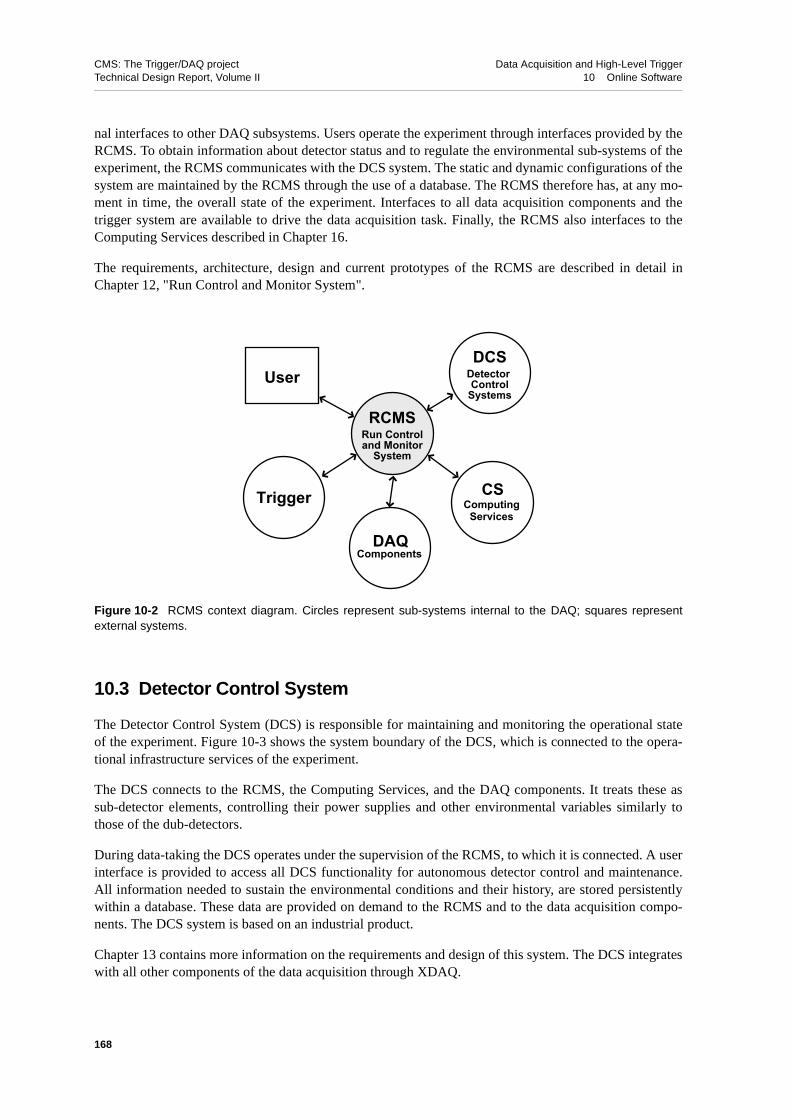
CMS: The Trigger/DAQ project Data Acquisition and High-Level TriggerTechnical Design Report, Volume II 10 Online Software
nal interfaces to other DAQ subsystems. Users operate the experiment through interfaces provided by theRCMS. To obtain information about detector status and to regulate the environmental sub-systems of theexperiment, the RCMS communicates with the DCS system. The static and dynamic configurations of thesystem are maintained by the RCMS through the use of a database. The RCMS therefore has, at any mo-ment in time, the overall state of the experiment. Interfaces to all data acquisition components and thetrigger system are available to drive the data acquisition task. Finally, the RCMS also interfaces to theComputing Services described in Chapter 16.
The requirements, architecture, design and current prototypes of the RCMS are described in detail inChapter 12, "Run Control and Monitor System".
10.3 Detector Control System
The Detector Control System (DCS) is responsible for maintaining and monitoring the operational stateof the experiment. Figure 10-3 shows the system boundary of the DCS, which is connected to the opera-tional infrastructure services of the experiment.
The DCS connects to the RCMS, the Computing Services, and the DAQ components. It treats these assub-detector elements, controlling their power supplies and other environmental variables similarly tothose of the dub-detectors.
During data-taking the DCS operates under the supervision of the RCMS, to which it is connected. A userinterface is provided to access all DCS functionality for autonomous detector control and maintenance.All information needed to sustain the environmental conditions and their history, are stored persistentlywithin a database. These data are provided on demand to the RCMS and to the data acquisition compo-nents. The DCS system is based on an industrial product.
Chapter 13 contains more information on the requirements and design of this system. The DCS integrateswith all other components of the data acquisition through XDAQ.
Figure 10-2 RCMS context diagram. Circles represent sub-systems internal to the DAQ; squares representexternal systems.
RCMSRun Controland Monitor
System
Detector Control
Systems
DCS
Trigger
User
CSComputing
Services
DAQComponents
168

CMS: The Trigger/DAQ project Data Acquisition and High-Level TriggerTechnical Design Report, Volume II 10 Online Software
10.4 Data Acquisition Components
The collection of DAQ components includes applications such as the distributed Event Builder (EVB),subdetector electronics configuration and monitoring components (FEC and FED), and software-basedtrigger-throttling mechanisms (aTTS). These applications require interfaces as shown in Figure 10-4, tothe Front-End Drivers, the trigger system, the high-level trigger services as well as the DCS. The relevant
Figure 10-3 DCS context diagram. Circles represent sub-systems internal to the DAQ; squares representexternal systems.
Figure 10-4 DAQ components interface. Circles represent sub-systems internal to the DAQ.
RCMSRun Controland Monitor
System
Detector Control
Systems
DCS
CSComputing
Services
Detectors
OperationalInfrastructure
Services
UserDAQ
Components
RCMSRun Controland Monitor
System
ComponentsDAQ
DCSDetectorControl
Systems
EventFilter
FEDFront-End
Driver
Trigger
CSComputing
Services
169

CMS: The Trigger/DAQ project Data Acquisition and High-Level TriggerTechnical Design Report, Volume II 10 Online Software
RCMS services connect to the data acquisition components to steer the data acquisition. Descriptions ofall data acquisition components involved in the event building process can be found in Part 2.
10.5 Cross-Platform DAQ Framework: XDAQ
An overview of the online software infrastructure based on XDAQ is shown in Figure 10-5. The frame-work provides basic system services such as memory management, communication services and the exec-utives in which applications are executed. Applications make use of these services in order to performtheir functions. Additional utility components provide support for hardware access, database access andother general-purpose interfaces such as the connection to the Detector Control System. Finally, high-lev-el tools support the configuration, control and monitoring of the system. These tools also include the userinterface that serves as the gateway to the data acquisition system. It is described in detail in Chapter 12,"Run Control and Monitor System".
An important decision in the design of the CMS DAQ system has been the adoption of a homogeneoussoftware infrastructure for all components in the DAQ. The decision is motivated by the expected ease ofintegration and configuration of multiple and diverse subsystems. The use of common and standardizedsoftware technologies reduces the effort associated with the maintenance and evolution of the systemover the long lifetime of the experiment.
The above can be realized with a domain-specific middleware [10-1] which is designed for data acquisi-tion and which offers its services through unambiguously defined interfaces. The role of this middlewareis to ease the tasks of designing, programming and managing applications by providing a simple, consist-ent and integrated distributed programming environment. Such a platform abstracts from the complexityand heterogeneity of the underlying distributed environment. The requirements, design and technologyfoundations of this approach are described in Chapter 11, "Cross-Platform DAQ Framework (XDAQ)".
Figure 10-5 Overview of the online software infrastructure.
Framework
Configuration, Control
Memory management,application execution environment,communication services formultiple networks
Event builder,FED readout, Trigger interface
Persistent data store access,hardware access, DCS interface
Resource service, control servicesinformation service, security service
Run Control application,simple control and monitoring client, scripting
Application components
Support components
Monitoring
170

CMS: The Trigger/DAQ project Data Acquisition and High-Level TriggerTechnical Design Report, Volume II 10 Online Software
10.6 References
10-1 P. Bernstein, “Middleware: A Model for Distributed Systems Services”, Communications of the ACM, 39 (196) 86.
171

CMS: The Trigger/DAQ project Data Acquisition and High-Level TriggerTechnical Design Report, Volume II 10 Online Software
172

CMS: The Trigger/DAQ project Data Acquisition and High-Level TriggerTechnical Design Report, Volume II 11 Cross-Platform DAQ Framework (XDAQ)
11 Cross-Platform DAQ Framework (XDAQ)
XDAQ is a framework designed specifically for the development of distributed data acquisition systems.It provides platform independent services, tools for local and remote inter-process communication, con-figuration and control, as well as technology independent data storage. To achieve these goals, the frame-work builds upon industrial standards, open protocols and libraries. This chapter starts by outlining theoverall requirements of XDAQ, and gives a description of its design followed by a summary of the devel-opment status.
11.1 Requirements
Three types of requirements have been identified: functional, non-functional and testing. The first catego-ry includes all requirements related to the functionality of the system, whereas the second category in-cludes all other requirements, with the exception of those related to the testing of the functionality andperformance of the DAQ. The requirements are outlined in the following sections.
11.1.1 Functional Requirements
11.1.1.1 Communication and Interoperability
The framework must provide a set of facilities for the transmission and reception of data within andacross subsystem boundaries. This functionality must be available for the communication both of applica-tions on the same processing unit and for tasks that are distributed over physically distinct interconnectedcomputers. Services must be available to retrieve all information that is needed to communicate to otherapplication components.
The software infrastructure must also provide mechanisms to ensure true interoperability among applica-tion components within the system without regard to the protocol used.
The framework shall foresee the possibility of interaction with new external systems through the provi-sion of facilities that allow the addition of communication protocols. These facilities shall be designedsuch, that no modifications in the applications that use the newly added communication method will berequired.
11.1.1.2 Device Access
Various system and application software components need a set of functions to access custom devices di-rectly for configuration and readout purposes. Access shall be provided in the same way for hardware de-vices that are directly connected to a computer as well as for devices that are accessed through busadapters. This software layer must also include provisions for extensions to new bus adapter products.These requirements imply additional constraints on the portability, robustness and efficiency of the soft-ware, as discussed in Section 11.1.2, "Non-Functional Requirements".
173

CMS: The Trigger/DAQ project Data Acquisition and High-Level TriggerTechnical Design Report, Volume II 11 Cross-Platform DAQ Framework (XDAQ)
11.1.1.3 Configuration, Control and Monitoring of Applications
The environment should provide the means to make the application parameters of any built-in or user-de-fined data types accessible to other applications within or outside the system. It shall therefore be possibleto inspect and modify all such parameters.
To allow the coordination of application components, it must be possible to define their overall behaviour,that is their states and modes. A mechanism should be in place to allow the specification of the tasks thatan application performs at a given time and which operations it accepts. In addition, services should beavailable to query and modify the state of applications.
A service must be present to record any structured information such as logging messages, error reports, aswell as complex data types. Examples include statistics and charts that are generated during run-time.Such information items, termed “documents”, should be disseminated to subscribing client processes.The introduction of documents necessitates the presence of mechanisms for their persistent and transientstorage. Documents can have a validity period after which they are discarded from the system and will nolonger be accessible to clients. It shall be possible to associate a priority with a document, which deter-mines the way in which it is processed and delivered to recipients.
The infrastructure must include facilities that allow the creation, maintenance, and persistent storage ofinformation about all hardware and software components that can be used. The data must cover all con-figuration that is necessary for the applications to perform their specified functions.
Applications will be able to share physical resources such as computers or networks. The framework mustsupport these operations by providing mechanisms to cope with allocation, sharing and concurrency con-ditions.
11.1.1.4 Re-usable Application Modules
The software infrastructure will include pre-built application components to perform the following tasks:
• Collection of data from a data link (see Section 7.3, "The Common Interface between the FEDsand the DAQ System")
• Event building according to the protocol described in Chapter 5, "Event Flow Control"
• Benchmarking of applications
• Diagnosis and validation of hardware and software components and their required functionalities
• Configuration, control and monitoring.
11.1.1.5 User Accessibility
In order to let a user interact with the system for configuration, control and monitoring purposes, a graph-ical user interface that is decoupled from the actual service implementations shall be provided. To per-form repetitively occurring tasks it shall be possible to define re-usable procedures that automate alloperations that the configuration, control and monitoring services offer.
174

CMS: The Trigger/DAQ project Data Acquisition and High-Level TriggerTechnical Design Report, Volume II 11 Cross-Platform DAQ Framework (XDAQ)
11.1.2 Non-Functional Requirements
This section describes constraints that are placed on the system in order to achieve its goals within the en-vironment in which it is embedded. The term “environment” includes the existing and foreseen hardwareinfrastructure, the data rate of the detector output, the lifetime of the experiment and various other issuesthat are not functions of the DAQ system.
11.1.2.1 Maintainability and Portability
Due to the variety of platforms that will be prevalent until the system is commissioned for operation, theinfrastructure must provide all the means to allow portability across operating system and hardware plat-forms. This includes support for accessing data across multiple bus systems and the possibility to add up-coming custom electronics to the set of supported systems without the addition or removal of explicitinstructions in user applications.
Operating system independence will be provided, but can only be maintained if applications do not direct-ly use native system functions. Most important, the memory management tools of the underlying systemshould not be applied directly, since their uncontrolled use may affect the robustness of the system. In ad-dition, the application code shall be invariant with respect to physical location and network. The rationalebehind the latter requirement is to improve system testability and maintainability. Users can create appli-cations in an environment with limited resources and move the validated application to the deploymentsystem without imposing changes in the software. Common functions should be independently packagedin re-usable building blocks. This leverages development, integration and testing efforts.
11.1.2.2 Scalability
The application domain is characterized by data transmission requirements. In order to meet the overallsystem requirements (see Chapter 2, "Requirements") and not to introduce unpredictable behavior, theoverhead introduced by the software must be constant for each transmission operation and must not affectthe data throughput in a significant way. Factors that might affect latency and throughput are memorymanagement, data copy operations and processing time that is proportional to the quantity of transmitteddata. The system shall have the ability to scale, that is to operate within the specified requirements and totake advantage of additional resource availability, as its size increases.
11.1.2.3 Flexibility
With respect to the various networks and protocols that are involved in the data collection tasks, it is nec-essary to allow the application developer to use multiple communication channels over different networksand protocols concurrently.
11.1.2.4 Identification
All system components will be unambiguously identified within the system for communication, controland tracking purposes.
175

CMS: The Trigger/DAQ project Data Acquisition and High-Level TriggerTechnical Design Report, Volume II 11 Cross-Platform DAQ Framework (XDAQ)
11.1.3 Testing Requirements
This section focuses on the requirements for testing the implementation of applications at the componentand system levels.
All application and framework components will be tested independently of each other. Integration tests ofcollaborating components must be performed and results validated against the functional requirements.Test data will be used as input to exercise components, subsystems and the system under normal and ab-normal operational conditions. These tests should be automated so that regression test procedures can beperformed on every newly released software.
A set of separate application modules to exercise performance and scalability measurements must be in-cluded in the software environment. Performance measurements will then be carried out to verify that thesystem satisfies all requirements and to investigate its behavior under high load.
The collection of all test software and its documentation includes verification checklists, test data as wellas supporting documentation like test plans, specifications, procedures, test cases, test data descriptionsand reports. Testing is planned and carried out within the organizational framework outlined inSection 11.3.
11.2 Design
This section describes the design of the software infrastructure, named XDAQ, in direct response to therequirements.
11.2.1 Executive Framework
The distributed programming environment follows a layered middleware approach [11-1], designed ac-cording to the object-oriented model and implemented using the C++ programming language [11-2]. Thedistributed processing infrastructure is made scalable by the ability to partition applications into smallerfunctional units that can be distributed over multiple processing units. In this scheme each computingnode runs a copy of an executive that can be extended at run-time with binary plugin components. Theprogram exposes two types of interfaces: “core” and “application”. The core interfaces lie between themiddleware and core plugin components, providing access to basic system functionalities and communi-cation hardware. Core plugins manage basic system functions on behalf of the user applications, includ-ing network access, memory management and device access. The application interfaces provide access tothe various functions offered by the core plugins and are placed between the middleware and the user ap-plication components as shown in Figure 11-1.
Middleware services include information dispatching to applications, data transmission, exception han-dling facilities, access to configuration parameters, and location lookup (address resolution) of applica-tions and services. Other system services include locking, synchronization, task execution and memorymanagement. Applications communicate with each other through the services provided by the executiveaccording to a peer-to-peer message-passing model. This allows each application to act both as a clientand a server. The general programming model follows the event driven processing scheme [11-3] wherean event is an occurrence within the system. It can be an incoming message, an interrupt, the completionof an instruction, like a direct memory access transfer, or an exception. Messages are sent asynchronouslyand trigger the activation of user-supplied callback procedures when they arrive at the receiver side. Eve-
176

CMS: The Trigger/DAQ project Data Acquisition and High-Level TriggerTechnical Design Report, Volume II 11 Cross-Platform DAQ Framework (XDAQ)
ry event therefore corresponds to a message that follows a standardized format. Initially, two formats aresupported. One is based on the I2O specification [11-4] and the other is XML [11-5].
The event-based processing model has been chosen because it is known to scale [11-6]. There is no needfor a central place in which the incoming data have to be interpreted completely. It is the responsibility ofeach software component that listens to a given type of event (e.g. data received, timeout) to decide whatit should do with the information received. Extensibility is thus achieved through the decoupling of thereception of a message and its processing. The procedure for a given message can be provided dynamical-ly during run-time by downloading a software module that contains all code to react to an incoming mes-sage of a given type. Furthermore it is possible to add new functionality by defining new messages. Thesystem provides a default procedure if for a given event no executable function has been supplied. Thismodel results in a homogeneous structure of software components with an intrinsic fault-tolerant behav-ior.
11.2.2 Application Interfaces and State Machines
One responsibility of the execution model is to keep track of the local states of all running applications.The overall behavior of an application in the scope of the executive framework can be modelled as a statemachine that is defined for each individual application. In order to facilitate the development of such in-terfaces, a common set of states and transitions is included with all applications and executives. Statechanges can be initiated by control commands that are sent to the applications and executives. The frame-work takes care of checking the consistency of the control commands. The success or failure of a statetransition is reported to the initiator of the request. The current state of an application is a parameter thatcan be queried at any time from an external system. Dependencies between applications, which rely onstate information are not foreseen and have to be managed by an external system (see Chapter 12, "RunControl and Monitor System").
The framework provides a mechanism, referred to as “reflection”, for the introspection of application in-terfaces in terms of exported variables and methods. Using this mechanism, an application can make var-
Figure 11-1 Middleware interfaces.
Coreplug-in
Core interfaces
Application interfaces
Applicationplug-in
Middlewareexecutive
177

CMS: The Trigger/DAQ project Data Acquisition and High-Level TriggerTechnical Design Report, Volume II 11 Cross-Platform DAQ Framework (XDAQ)
ious data elements visible to external systems. Both simple built-in data types as well as user-definedcomposite data structures are supported and the set of data types that are exported can be extended by theuser. All functions defining the control interface of an application can be retrieved at run-time. This ena-bles integration with external systems without the need to obtain a written specification of the applicationinterface.
11.2.3 Memory Management
The executive program provides applications with efficient memory management facilities. These arebased on a scheme called “buffer-loaning” which avoids fragmentation of memory over long run periodsand presents a safe operation model that prevents extensive growth of memory consumption. With thebuffer-loaning scheme, applications or core-plugins ask the executive for fixed sized chunks of memoryfrom one of various buffer pools. The principle is displayed graphically in Figure 11-2.
The executive manages various types of pools, including ordinary user-space memory, a reserved amountof physical memory (e.g. the Linux “bigphys” kernel extension) and memory on network cards. The poolscan be configured such that exceptions are raised if too little memory is available. All memory buffers areallocated from the available pool and are accessible through a reference that can be further lent to othersoftware components. For example, a user application prepares a message and passes it on to a transportcomponent that handles the network transmission. Eventually, the buffer must be returned to its pool.Built-in reference counting ensures that a buffer is not returned into its originating pool before the verylast user has released it.
Various buffers can be chained together to allow arbitrarily sized data. The mechanism not only enablesefficient zero-copy implementations, but also provides the foundation for transparent operation acrossnetwork boundaries. Various high-speed interconnects and custom built electronics rely on non-standardmemory models, that would otherwise require the instrumentation of user programs with special instruc-tions. Buffer pools can be added to the executive to offer specific allocation through an interface that iscommon to all memory types.
Figure 11-2 Illustration of the buffer-loaning mechanism. A task loans a reference to an unused buffer thatmatches the closest requested data size from a buffer pool (step 1). The buffer can be passed to another task byforwarding the buffer reference (step 2) without copying the data. The buffer is released to the pool by destroy-ing the buffer reference (step 3). It can now be re-allocated to another task.
Buffer pool
Buffer reference
Task A Task B
Step 1 Step 2 Step 3
178

CMS: The Trigger/DAQ project Data Acquisition and High-Level TriggerTechnical Design Report, Volume II 11 Cross-Platform DAQ Framework (XDAQ)
11.2.4 Data Transmission
Data transmission in the described distributed programming environment is carried out by special appli-cation components, named peer transports (see Figure 11-3). Peer transports register themselves with theexecutive as being capable of resolving addresses as well as transmitting and receiving data.
Communication between ordinary applications is accomplished by means of an executive function. Thisfunction, when invoked, re-directs the outgoing message to the proper peer-transport that in turn deliversthe data over the associated medium. In this way the framework is independent of any transport protocolor network and can be extended at any time to accommodate newly appearing communication technolo-gies.
The baseline framework includes a number of peer-transports which are listed in Table 11-1. Applicationscan communicate according to two different models, unicast and multicast. Unicast is designed for trans-mitting data to a single destination, whereas multicast provides efficient handling of group communica-tion within a network. The model extends a single line of communication over a network allowingmessages to be sent simultaneously to a group of applications, i.e. all instances of a given class. If apeer-transport does not have the capability to perform true multicast (e.g. TCP/IP), it can tell the execu-tive that it will emulate the required behaviour using normal point-to-point message exchange. This is animportant feature to allow the verification of software in an environment with limited functionalities.
Figure 11-3 Communication over multiple networks through peer-transports.
Middlewareexecutive 1
Middlewareexecutive 3
Peer Transport type: Myrinet
Peer Transport type: TCP/IP
Middlewareexecutive 2
179

CMS: The Trigger/DAQ project Data Acquisition and High-Level TriggerTechnical Design Report, Volume II 11 Cross-Platform DAQ Framework (XDAQ)
11.2.5 Protocols and Data Formats
The framework supports two data formats, one based on the I2O specification and the other on XML. I2Omessages are datagrams with a maximum size of 256 kB. For sizes larger than this maximum, the datahave to be split and sent in a sequence of multiple frames. The framework provides mechanisms to per-form this task. I2O messages are primarily intended for the efficient exchange of binary information, e.g.data acquisition flow. No interpretation of such messages takes place in the executive. The messages areused directly by the applications to perform the required computation tasks. However, the content is plat-form-dependent and the application designer must obey all alignment and byte-ordering rules. Moreover,the structures for I2O messages are provided through C language definitions and a recompilation of thecorresponding applications is required if the data content type changes. The use of the I2O messageframes can be combined with the buffer-loaning memory allocation scheme to create efficient applica-tions. Thus, data that have been received do not need to be copied before they are passed on, since it issufficient to work with references to the corresponding frames.
Despite its efficiency the I2O scheme is not universal and lacks flexibility. A second type of communica-tion has been chosen for tasks that require higher flexibility such as configuration, control and monitor-ing. This message-passing protocol, called Simple Object Access Protocol (SOAP) [11-7] relies on thestandard Web protocol (HTTP) [11-8] and encapsulates data using the eXtensible Markup Language(XML) [11-5]. The adoption of SOAP naturally leads to the use of Web Services that standardize the wayin which applications export their interfaces to possible clients[11-9]. The executive middleware exposesan interface to the application programmer that is based on the JAXM package [11-10] from Sun Mi-crosystems and implements the W3C SOAP 1.1 specification for creating and parsing SOAP messages.Clients can use any SOAP-compliant communication package to interact with the executives and their ap-plication module plug-ins. This approach has several advantages over the transmission of statically de-clared, binary messages. First, the availability of a standardized interface to inspect and manipulate XMLdata, called the Document Object Model (DOM) [11-11] helps to quickly integrate the applications with avariety of data sources. XML data can be read from disk or remote Web sites; they can be processed by anumber of tools for the majority of operating systems, they are machine and human readable and can betransmitted over any kind of transport protocol. XML data are understood across platform boundaries, be-cause data are plain text and through the association of a grammar, it is possible to describe the contentsof a message. Second, XML favors system robustness through the use of grammars and named elementsthat allow detection of malformed messages. Third, XML allows scalable configuration, monitoring andcontrol, by avoiding large quantities of data to be sent across the network at once. Messages may containlinks to data that can be resolved when needed. Applications may export information by transmitting anXML structure with the link to the location at which they have placed the generated data. It is importantto note that there is no limit to the data content type. Any text, binary or complex structure can be de-
Table 11-1 Baseline peer-transports.
Transport technology Description
TCP/IP reliable messages over various physical networks
UDP (unicast and native multicast) unreliable datagrams over various physical networks
SOAP (HTTP messaging with XML data) reliable delivery of XML documents over various physical networks
local FIFO communication among applications within the same executive
GM reliable messaging over Myrinet
raw Ethernet (unicast and true multicast) unreliable messages over Ethernet (VxWorks operating system only)
180

CMS: The Trigger/DAQ project Data Acquisition and High-Level TriggerTechnical Design Report, Volume II 11 Cross-Platform DAQ Framework (XDAQ)
scribed in XML and any kind of protocol can be chosen to transmit these data. The framework supportsan initial small set of data structures that can be extended gradually with additional capabilities (seeTable 11-2).
11.2.6 Application Components
In addition to the services that support distributed computing, the online software framework includescomponents that facilitate the building of data acquisition systems including general tasks like hardwareaccess, database access and local data monitoring. These components are intended to be used in four do-mains:
• the global DAQ system of the experiment
• local DAQ systems
• the development and production environment of the FED
• testbeam DAQ systems
11.2.6.1 Data Acquisition Components
The online software infrastructure provides re-usable application components to perform event buildingaccording to the protocols described in Chapter 5, "Event Flow Control". This includes generic softwarefor the Readout Unit (RU), Builder Unit (BU) and Event Manager (EVM) subsystems. The event buildercomponents form a distributed application that can be configured to run on a set of networked computers.The application exposes three distinct interfaces: input from the detector readout, output to the High-Lev-el Trigger system and input from the trigger system. In addition to the event builder, the software includesthe application components necessary for the readout through the front-end links as well as the handlingof trigger information.
The DAQ software components serve as building blocks for the local DAQ systems, where they can beused for commissioning part of the DAQ itself, and also for calibration and detector monitoring purposes.However, they may need adaptation to meet additional requirements that are specific to the operationalenvironment. A similar procedure applies to testbeam and FED development applications.
11.2.6.2 Common Application Components
Components are included, to be used from within applications, to ease direct hardware access, persistentdata store operations, communication with DCS and local monitoring.
Table 11-2 Some data types that XDAQ can export through XML messages.
Data type Example
simple types (built-in C++ native types) unsigned long, float, string
vectors of simple or composite types vector<int>, vector< vector <string> >
bags of simple types (collections of types) (unsigned long, float, vector<string>)
JAS [11-12] plot types a histogram, including error bars
181

CMS: The Trigger/DAQ project Data Acquisition and High-Level TriggerTechnical Design Report, Volume II 11 Cross-Platform DAQ Framework (XDAQ)
The hardware access library is used to directly manipulate hardware devices for configuration purposes. Itprovides access to registers and memory areas for various bus systems through named objects that can bedefined dynamically at run-time.
The database access library exhibits an interface to read information from persistent data stores and topresent it to the user through the standardized Document Object Model (DOM) of the World Wide WebConsortium (W3C). The DOM renders information as trees that can be traversed by the application code.Each node can contain a named data element or may be a link to other information that is accessiblethrough one of the provided protocols. The library provides the required authentication and access regula-tion procedures for each type of persistent data store that is supported. No particular requirements are im-posed on the database schema for using this package. The baseline framework provides support forOracle [11-13], MySQL [11-14] and the file system.
The DCS access component enables applications in the online environment to communicate with the ex-periment’s Detector Control System. Any control system that has been built with the PVSS-II SCADA[11-15] product can be seen by an application through this component as just another application compo-nent. Conversely, an application in the online domain can be seen by the PVSS-II system as soon as it reg-isters with the system. Thus, bi-directional communication between the DAQ and DCS domains isachieved. The interface between the two systems is described in detail in [11-16]. An online applicationcomponent can read and write values and subscribe for change notifications. The PVSS-II system canread and modify values that are made visible by an online application. The PVSS-II system can also re-quest to be notified when value changes occur, but it is left to the designer of the online application to ex-plicitly respond to such a request. The PVSS-II system may also access the interface of a registeredapplication in order to invoke actions on them. Provision of functionality to perform the described taskswith the PVSS-II system belongs to the DCS domain.
The data monitoring library is used to perform basic statistical analysis for monitoring application andsystem operation on a local processing node. It allows the structuring of the results for storage with data-base systems or for external visualization toolkits.
11.2.7 Configuration, Control and Monitoring Components
Configuration, control and monitoring correspond to tasks that affect the distributed programming envi-ronment and the applications that run in it. All three tasks involve components both in the executive pro-grams and in the applications. The configuration of the executives comprises all information that isneeded in order to
• identify which applications must be run in a certain executive
• communicate to other executives and applications, including external subsystems
• find the location of the binary objects needed for all described tasks.
The configuration of the applications is limited to providing default values for their exported parameters.
To manage configuration data, a service that keeps track of all hardware and software resources is provid-ed. This service acts as a database and does not yet allow the control and configuring of the running sys-tem. This will be carried out by control services. “Control” in this context is defined as all the actionsnecessary for the deterministic execution of state transitions that have been defined for the executive andall configured applications. These services are responsible for initiating state transitions in executives andapplications, thus including the issuing of configuration commands (see Section 12.3.1, "State Definitionsand System Synchronization").
182

CMS: The Trigger/DAQ project Data Acquisition and High-Level TriggerTechnical Design Report, Volume II 11 Cross-Platform DAQ Framework (XDAQ)
“Monitoring” corresponds to the collection of data that have been made visible by the executives and ap-plications through exported parameters or supplied functions that can be invoked through their corre-sponding messages. Two modes are supported:
• pull mode: the collection of data is performed by repetitive inquiry of the involved components
• push mode: all components actively send data to the monitoring service
The software infrastructure provides the basic primitives to implement application-specific monitoringthrough the Information Service as described in Section 12.4.4, "Information and Monitor Service(IMS)".
11.3 Software Process Environment
The process via which the evolution of the system occurs in an orderly fashion is termed the softwareprocess. It is an iterative process of synthesis, development and operation of the software that satisfies ina near-optimal manner the full range of requirements for the system and thus helps to increase the likely-hood of being successful.
The development of the CMS online software has adhered to established standards of software processes.A short summary of the main elements is provided here.
11.3.1 Documentation Guidelines and Procedures
Guidelines based upon existing standards are being defined to provide support for the documentation ofthe system under development, including all artifacts developed during the life cycle of the project. Theformat, content and categories of documents for the software process and development shall be defined.Guidelines will help in preparing technical documentation, provide a reference for uniformity of style,format and content, with the goal of enhancing consistency of documentation and visibility into the com-pleteness of the project.
11.3.2 Configuration Management Tools
Configuration management is supported by various tools that are freely available. CVS [11-17] is a wide-ly used tool for version management and GNU Make [11-18] is a tool for system building. Both of theseare normally supplied with the UNIX system. Configuration management relies on a database that recordsinformation about system changes and change requests that are outstanding. It also requires some formalmeans of requesting changes. A combination of CVS and the SourceForge.net [11-19] facilities fit theseneeds. Distribution of the software to end users is accomplished through a packaging and installation toolthat must be capable of covering all platforms supported by the software. Currently InstallAnywhere isused for this purpose [11-20]. In addition, CVS server access is granted to users that require immediateupdates. These include co-developers from remote institutes and users with the need for tailored compo-nents, e.g. testbeam applications.
183

CMS: The Trigger/DAQ project Data Acquisition and High-Level TriggerTechnical Design Report, Volume II 11 Cross-Platform DAQ Framework (XDAQ)
11.3.3 Software Development Environment
The online-software is based on various existing industry standards to reduce development and mainte-nance efforts as well as to achieve interoperability with external systems. The selected technologies in-crease the probability of achieving these goals, but cannot guarantee success by themselves. A firmunderstanding of the technologies is required together with expertise in system integration.
The implementation language of the executive and its application components is C++. The reasons under-lying this decision are fourfold. First, the distributed programming environment has been designed ac-cording to the object-oriented model and C++ maps well to this approach. Second, C++ is theimplementation language of the offline reconstruction framework. Hence, integration with high-level trig-ger code that is based on the offline software interfaces is facilitated. Third, the online software environ-ment relies on efficient program execution that can at present only be achieved with compiled binaryexecutables. Fourth, C++ is fully integrated with C, the systems programming language of the majority ofoperating systems. The currently supported platforms are listed in Table 11-3. Configuration, control andmonitoring services are currently implemented in Java and are therefore available on any Java enabledplatform..
The software is available for, but not limited to the Linux (Red Hat distribution), Mac OS X (Apple Inc.),Solaris (Sun Microsystems) and VxWorks (Wind River) operating systems. VxWorks is a real-time sys-tem that finds its deployment wherever requirements occur that cannot be met by a time-sharing operatingsystem, such as the UNIX family. This includes rapid prototyping of embedded environments and its usein highly constrained environments. VxWorks has been chosen because of its capabilities to be tailored toa variety of hardware platforms, its proven efficiency and wide acceptance in industry. Solaris and Linuxare two major players in the UNIX marketplace and excel through the vast amounts of documentation.Last but not least, most third party products to which the online software infrastructure has to interfaceare supported on these target platforms. All what has been said for Solaris and Linux also applies to theMacOS X platform. In addition, a variety of software development and system administration tools areavailable that exploit the full range of functions that this system provides.
For processing SOAP messages, use is made of the freely available Xerces parser from the Apacheproject [11-21] library that implements the Document Object Model (DOM) interface for manipulatingXML data in C++ and Java. DOM is a W3C (Word Wide Web Consortium) standard that defines lan-guage bindings for various programming languages including C++ and Java.
Relational databases have proven robustness and scalability, and have therefore been selected as the pri-mary means for persistently storing configuration data in the online software environment. The marketalso suggests that these products will be around for the entire lifetime of the experiment. The format ofthe data entered into and retrieved from different database products has been normalized to XML andDOM. This design choice allows the development of applications independently of the database
Table 11-3 Platforms and languages currently supported by the online software infrastructure.
Type of software Platform Languages/Compilers
Executive and application components
Sun/Solaris on Sparc processors,Linux on Intel processors,Mac OS X on PowerPC processors,VxWorks on Intel and PowerPC processors
C++/GNU g++, C/GNU gcc
Configuration, control and monitoring services
Any Java/Tcl enabled platform Java/Sun JDK, Tcl
184

CMS: The Trigger/DAQ project Data Acquisition and High-Level TriggerTechnical Design Report, Volume II 11 Cross-Platform DAQ Framework (XDAQ)
back-end. The online software infrastructure presently supports the following back-end technologies: Or-acle, mySQL, file system and native XML databases[11-22][11-23].
The software infrastructure includes a graphical user interface, entirely written in Java, which serves sim-ple configuration, control and monitoring purposes. It uses the JAXM [11-10] package for performingSOAP communication and interfaces to the Java Analysis Studio (JAS) [11-12] to demonstrate the capa-bilities of interfacing to third party products through the XML language. Scripting is supported in thesimple control program through a built-in Tcl language interpreter [11-24]. No limitation exists on the useof other scripting languages for interfacing to the distributed programming environment as long as SOAPcommunication is available.
11.4 System Management
These tools are intended to manage the set of all computers that make up the DAQ system. The manage-ment functions include installation of the operating system, installation and upgrade of the applicationsoftware as well as the boot strap process. A secondary function is the continuous monitoring of the com-puting infrastructure. Detailed information can be found in Section 16.6.1, "Cluster Management".
11.5 Prototype Usage and Experience
Various prototypes of the described software infrastructure have been used in testbeam environments forthe Muon and Tracker subsystems. The gathered experience served as an input for additional require-ments and technology decisions. The software is also actively used in FED development projects and forthe preparation of front-end configuration systems.
In addition, the software infrastructure has been installed at institutes that participate in the developmentof the DAQ system. At CERN, the software environment serves as an infrastructure for DAQ systemevaluation (see Section 7.7, "Readout Column Prototypes and Test-benches") and for integration taskswith the high-level trigger processing framework (see Section 8.6, "Prototypes and Results"). For a de-tailed analysis and basic efficiency measurements of the communication subsystem implemented inXDAQ, see [11-25]. The existing downscaled DAQ column prototype proves that the design can be suc-cessfully applied in a “real-world” environment and that there are no observable deficiencies introducedby the chosen technologies. In the context of design, the prototype also shows that the correct balance hasbeen made between flexibility and efficiency.
The deployment of the software in various real scale application scenarios demonstrated the viability ofthe approach taken. The following sub-sections outline two of these applications, the tracker local DAQsystem for front-end control and calibration, and the muon chamber validation system.
11.5.1 Tracker Testbeam
The silicon microstrip detectors are readout via an analog optical link connected to the analog to digitalconverters of the FED. The control commands for the front-end chips, together with the clock and level 1trigger, are propagated to the detectors through a proprietary token-ring network. This task is carried outby a Front-End Controller (FEC) interacting with several communication and control units (CCUs). Com-missioning of detectors is a dedicated data acquisition task including the communication channel de-
185
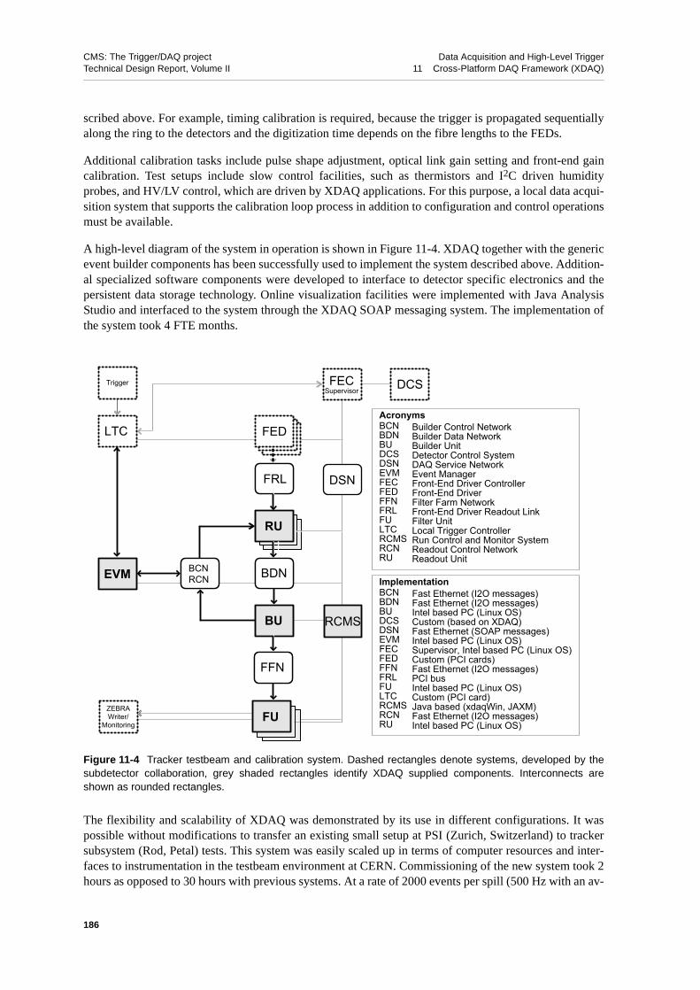
CMS: The Trigger/DAQ project Data Acquisition and High-Level TriggerTechnical Design Report, Volume II 11 Cross-Platform DAQ Framework (XDAQ)
scribed above. For example, timing calibration is required, because the trigger is propagated sequentiallyalong the ring to the detectors and the digitization time depends on the fibre lengths to the FEDs.
Additional calibration tasks include pulse shape adjustment, optical link gain setting and front-end gaincalibration. Test setups include slow control facilities, such as thermistors and I2C driven humidityprobes, and HV/LV control, which are driven by XDAQ applications. For this purpose, a local data acqui-sition system that supports the calibration loop process in addition to configuration and control operationsmust be available.
A high-level diagram of the system in operation is shown in Figure 11-4. XDAQ together with the genericevent builder components has been successfully used to implement the system described above. Addition-al specialized software components were developed to interface to detector specific electronics and thepersistent data storage technology. Online visualization facilities were implemented with Java AnalysisStudio and interfaced to the system through the XDAQ SOAP messaging system. The implementation ofthe system took 4 FTE months.
The flexibility and scalability of XDAQ was demonstrated by its use in different configurations. It waspossible without modifications to transfer an existing small setup at PSI (Zurich, Switzerland) to trackersubsystem (Rod, Petal) tests. This system was easily scaled up in terms of computer resources and inter-faces to instrumentation in the testbeam environment at CERN. Commissioning of the new system took 2hours as opposed to 30 hours with previous systems. At a rate of 2000 events per spill (500 Hz with an av-
Figure 11-4 Tracker testbeam and calibration system. Dashed rectangles denote systems, developed by thesubdetector collaboration, grey shaded rectangles identify XDAQ supplied components. Interconnects areshown as rounded rectangles.
LTC
Trigger
RU
EVM
BU
BDNBCNRCN
FU
FFN
FRL
FECSupervisor
ZEBRAWriter/
Monitoring
DCS
RCMS
DSN
FEDAcronymsBCNBDNBUDCSDSNEVMFECFEDFFNFRLFULTCRCMSRCNRU
Builder Control NetworkBuilder Data NetworkBuilder UnitDetector Control SystemDAQ Service NetworkEvent ManagerFront-End Driver ControllerFront-End DriverFilter Farm NetworkFront-End Driver Readout LinkFilter UnitLocal Trigger ControllerRun Control and Monitor SystemReadout Control NetworkReadout Unit
ImplementationBCNBDNBUDCSDSNEVMFECFEDFFNFRLFULTCRCMSRCNRU
Fast Ethernet (I2O messages)Fast Ethernet (I2O messages)Intel based PC (Linux OS)Custom (based on XDAQ)Fast Ethernet (SOAP messages)Intel based PC (Linux OS)Supervisor, Intel based PC (Linux OS)Custom (PCI cards)Fast Ethernet (I2O messages)PCI busIntel based PC (Linux OS)Custom (PCI card)Java based (xdaqWin, JAXM)Fast Ethernet (I2O messages)Intel based PC (Linux OS)
186

CMS: The Trigger/DAQ project Data Acquisition and High-Level TriggerTechnical Design Report, Volume II 11 Cross-Platform DAQ Framework (XDAQ)
erage event size of 20 kB), a maximum data throughput of 100 Mb/s was achieved, which corresponds tothe available Fast Ethernet capabilities. During one operation, that consisted of five days of continuousand uninterrupted data taking, around 600 GB of data were produced for analysis. Users gave positivefeedback on the simple interface for controlling the distributed system. It was noted that novices couldeasily operate and configure the system themselves, in particular the application of configuration changesto re-distribute processing tasks to multiple computers.
11.5.2 Muon Chamber Validation
The 250 chambers that make up the muon barrel spectrometer need to be tested through cosmic ray acqui-sition runs before shipping to and after their arrival at CERN. Tests with muon beams at high data ratestogether with coupling to other subdetectors are also necessary to validate the detector behavior under re-alistic conditions. The observables include occupancy calculations for determining the particle hits foreach channel, drift time histograms and the response to dedicated test pulse events. Thus, a data acquisi-tion system had to be put in place to perform these tasks. XDAQ was used as the generic platform to im-plement this system. As outlined in Figure 11-5, the software required customization of three parts, thelocal trigger controller (LTC), readout of custom electronics through the VME bus and interfacing to adata storage/analysis back-end. For the acquisition task, the generic event builder components were used.Run control was implemented by the prototype system as described in Section 12.6.1, "RCMS for SmallDAQ Systems". As opposed to the tracker experience, slow control was performed by a separate, Win-dows based system.
Figure 11-5 Muon testbeam and validation system. Dashed rectangles denote systems, developed by the sub-detector collaboration, grey shaded rectangles identify XDAQ supplied components. Interconnects are shownas rounded rectangles.
LTC
Trigger
FED
RU
EVM
BU
BDNBCNRCN
FRL
Monitoring
RCMS
FileSystemStorage
AcronymsBCNBDNBUDSNEVMFEDFRLLTCRCMSRCNRU
Builder Control NetworkBuilder Data NetworkBuilder UnitDAQ Service NetworkEvent ManagerFront-End DriverFront-End Driver Readout LinkLocal Trigger ControllerRun Control and Monitor SystemReadout Control NetworkReadout Unit
DSN
ImplementationBCNBDNBUDSNEVMFEDFRLLTCRCMSRCNRU
Fast Ethernet (I2O messages)Fast Ethernet (I2O messages)Intel based PC (Linux OS)Fast Ethernet (SOAP messages)Intel based PC (VxWorks OS)Custom (VME cards)VME busCustom (PCI card)Actual CMS prototypeFast Ethernet (I2O messages)PC (Linux) or VME CPU (VxWorks)
187
CMS: The Trigger/DAQ project Data Acquisition and High-Level TriggerTechnical Design Report, Volume II 11 Cross-Platform DAQ Framework (XDAQ)
A similar setup was used during a test period in 2001 for the Gamma Irradiation Facility (GIF) facility atCERN. In this case, a muon chamber was coupled to a RPC detector and a beam chamber to verify the si-multaneous response of the RPC and muon chambers. Update of the existing system went smoothly.
As a result of this project, several requirements were identified, mainly covering configuration, controland monitoring. Hardware platform heterogeneity (different bus systems, byte ordering and data align-ment rules), as well as the presence of two different operating systems platforms, posed a challenge to theinteroperability among all system components. The supported platforms included PowerPC based VMEprocessors running the VxWorks real-time operating system, and Intel based personal computers withboth Linux and VxWorks.
The provided abstraction fitted the need to switch between processor and operating system types withoutextra work. The required event rate of 10 kHz and the peak output of 4 MB/sec were well absorbed by thehardware and software installation in place. The variance of the event sizes stressed the buffer manage-ment system of XDAQ and thus proved the robustness of the design. Uptime measured over two weekswas 60%, including penalties from changing hardware configurations. From the initial intent to create thesystem to its completion, including the learning phase, six man months had to be invested. A system de-veloped from scratch in the same time scale would not have provided the seamless integration with laterappearing components (e.g. silicon beam telescope) and the ability to efficiently carry out modificationsand configuration changes.
Through these experiences, confidence has been gained that the proposed design of the software infra-structure can fulfill the enumerated requirements.
11.6 Summary and Conclusions
This sub-section summarises the present status of the XDAQ framework development. The existing soft-ware is a proof of concept of the proposed design. The working prototype has limited functionality thatcovers the minimum requirements for demonstrating a simple data acquisition system. Confidence hasbeen gained through the use of the software in test beams and laboratory environments such as the DAQcolumn that such a design approach can be scaled to the final data acquisition system. All dimensions ofthe system were investigated from readout and network communication to the graphical user interface forcontrol and configuration.
A C++ framework has been developed that incorporates preliminary support for binary message-passingfollowing the I2O standard, and SOAP messages for platform independent communication. In this contextseveral technologies have been exercised, including Apache Xerces for the DOM representation of XMLmessages, and Java web services for interfacing to users and external systems. Pre-production peer trans-ports for network communication on all supported platforms (Intel based Linux, Power PC Mac OS X,and Power PC and Intel based VxWorks) now exist for TCP/IP, UDP and a subset of HTTP. FIFO com-munication supports applications running within the same XDAQ executive/process. A peer transport in-terfacing Myrinet GM has been implemented for tests on Intel based Linux PCs, as well as a simple peertransport for testing raw Ethernet communication on VxWorks to support the muon testbeam. A libraryfor direct hardware access for PCI and VME devices has been implemented for the Linux operating sys-tem. A Linux driver together with a XDAQ application component to interface the generic PCI card forreading out FED devices has also been developed.
A prototype application component for interfacing XDAQ applications to various databases technologiesin a standard but technology independent manner has been developed. The component currently supportsMySQL, Oracle 8i and the file system. A user interface has been written in Java to exercise access (con-
188

CMS: The Trigger/DAQ project Data Acquisition and High-Level TriggerTechnical Design Report, Volume II 11 Cross-Platform DAQ Framework (XDAQ)
trol and configuration) to a XDAQ distributed system through SOAP messages. Two prototype eventbuilder applications have been developed to test and study two event builder protocols that are currentlyused for test beam systems. A third event builder is being developed for the fully functional data acquisi-tion system.
The implementation of the presented design requires a significant development effort. All the requiredfunctionalities outlined in this section must be put in place with the level of robustness that ensures theproper operation of the CMS data acquisition system. The proposed layered architecture of the XDAQmiddleware will allow the porting of all application components to other platforms, should that becomenecessary.
11.7 References
11-1 P. Bernstein, “Middleware: A Model for Distributed Systems Services”, Communications of the ACM, 39 (1996) 86.
11-2 J. Gutleber and L. Orsini, “Software Architecture for Processing Clusters Based on I2O”, Cluster Computing 5(1):55-65, Kluwer Academic Publishers, 2002.
11-3 B.N. Bershad et al.,”Extensibility, Safety and Performance in the SPIN Operating System”, in Proceedings of the Fifteenth ACM Symposium on Operating System Principles, pp. 267-284, 1995.
11-4 I2O Special Interest Group, Intelligent I/O (I2O) Architecture Specification v2.0, 1999, at http://www.intelligent-io.com
11-5 J. Boyer, “Canonical XML Version 1.0, W3C Recommendation 15 March 2001”, http://www.w3.org/TR/xml-c14n
11-6 P. Pardyak and B.N. Bershad, “Dynamic binding for an extensible system”, in Proceedings of the 2nd USENIX Symposium on Operating Systems Design and Implementation, 1996, pp. 201-212.
11-7 D. Box et al.,” Simple Object Access Protocol (SOAP) 1.1, W3C Note 08 May 2000”, http://www.w3.org/TR/SOAP
11-8 R. Fielding et al.,”Hypertext Transfer Protocol - HTTP /1.1”, IETF RFC 2616, June 1999, http://www.w3.org/Protocols/rfc2616/rfc2616.html
11-9 G. Glass, ”Web Services: building blocks for distributed systems”, Prentice Hall, 2002.
11-10 “Java API for XML Messaging (JAXM) Specification v1.0”, Sun Microsystems, 901 San Antonio Road, Palo Alto, California 94303, USA, October 2001.
11-11 A. Le Hors et al.,”Document Object Model (DOM) Level 3 Core Specification, Version 1.0, W3C Working Draft 13, September 2001”, http://www.w3.org/TR/2001/WD-DOM-Level-3-Core-20010913
11-12 The Java Analysis Studio, http://jas.freehep.org
11-13 Oracle database product documentation: http://oradoc.cern.ch, provided by the CERN Oracle support (http://wwwinfo.cern.ch/db/oracle/)
11-14 The MySQL open source database: http://www.mysql.com/
11-15 The PVSS II system from ETM provided through the CERN IT division, http://itcobe.web.cern.ch/itcobe/Services/Pvss/
11-16 DCS-DAQ Interface Requirements, see http://cern.ch/xdaq
189

CMS: The Trigger/DAQ project Data Acquisition and High-Level TriggerTechnical Design Report, Volume II 11 Cross-Platform DAQ Framework (XDAQ)
11-17 Concurrent Versions System, http://www.cvshome.org/
11-18 GNUMake project, http://www.gnu.org/software/make/make.html
11-19 http://sourceforge.net/projects/xdaq/ , hosted by the Open Source Development Network, 50 Nagog Park Acton, MA 01720, USA.
11-20 Zero G Software Inc., 514 Bryant Street, San Francisco, CA 94107, USA. See also http://www.zerog.com
11-21 Apache Software Foundation XML project, http://xml.apache.org
11-22 Exist DB, http://exist.sourceforge.net and Apache XIndice, http://xml.apache,org/xinidice
11-23 http://www.xmldb.org
11-24 R. Johnson, “Tcl and Java integration”, Sun Microsystems Laboratories, 901 San Antonio, MS UMTV-29-232, Palo Alto, CA 94303-4900, USA, 1998. See also http://www.tcl.tk/software/java
11-25 J. Gutleber et al.,”Architectural Software Support for Processing Clusters”, in Proceedings of the IEEE International Conference on Cluster Computing, pp. 153-161, November 28 - December 1, 2000, Chemnitz, Germany, IEEE Computer Society Press, Los Alamitos, California.
190

CMS: The Trigger/DAQ project Data Acquisition and High-Level TriggerTechnical Design Report, Volume II 12 Run Control and Monitor System
12 Run Control and Monitor System
The Run Control and Monitor System (RCMS) is the collection of hardware and software components re-sponsible for controlling and monitoring the CMS experiment during data taking. It provides physicistswith a single point of entry to operate the experiment and to monitor detector status and data quality. Theinterface enables users to access and control the experiment from any part in the world providing a “virtu-al counting room”, where physicists and operators can perform all programmable actions on the system,effectively taking shifts from a distance.
In order to achieve its goals, the RCMS interoperates with the Detector Control System (DCS), the dataacquisition components and the trigger subsystem as shown in Figure 10-2, through the services providedby the distributed processing environment (see Section 10.5, "Cross-Platform DAQ Framework:XDAQ"). For configuration, user administration and logging, the RCMS makes use of a database man-agement system.
The RCMS is the master controller of the CMS DAQ when the experiment is taking data. It instructs theDetector Control System (DCS) to act according to the specific needs of a data-taking session.
The three main functions of the RCMS are
• control and monitoring with the support of the DCS to ensure the correct and proper operation ofthe CMS experiment
• control and monitoring of the data acquisition system
• provide user interfaces and allow users to access the system from anywhere in the world
The RCMS views the experiment as a set of partitions when performing these three functions. A partitionis the smallest grouping of entities that can be configured and operated independently. This includes con-figuration, monitoring, error handling, logging and synchronization with other subsystems.
The RCMS architecture faces similar requirements to applications in the Internet world, in particular:
• connecting many clients distributed in a large geographical area to a set of servers and databases
• providing secure access
• scaling up in terms of connectivity to the servers and transactions per second of the databases
The design and prototyping of the RCMS has followed these rapidly developing environments. Many ofthese widely-spread software tools follow an open-source approach, thus facilitating the integration withother software packages. As discussed later in this chapter, it is planned to maximise the use of standardsoftware technologies in the RCMS.
12.1 Requirements
This section presents the requirements of the RCMS grouped by the following functionalities: configura-tion, control and monitoring. It also includes the requirements for the user interface.
191

CMS: The Trigger/DAQ project Data Acquisition and High-Level TriggerTechnical Design Report, Volume II 12 Run Control and Monitor System
12.1.1 Configuration Requirements
The system will provide means for defining and storing persistently the configuration of any subsystemand collections of subsystems. It shall be possible to retrieve and apply stored configurations. The systemmust also support run-time inspection and modification.
The RCMS views the experiment as a collection of partitions, where a partition is the smallest configura-ble grouping of units. The use of partitions satisfies the requirement that independent sections of the ex-periment can be run concurrently. In order to support partitions, the following requirements must be met:
• It must be possible to define, configure, control and monitor any possible partition of the CMS ap-paratus.
• Multiple partitions can run concurrently. Resources can be allocated to and shared between multi-ple partitions.
• It must be possible to store and retrieve all partition configurations to and from persistent storage.
• It must be possible to group several resources into a partition according to a set of pre-definedrules. Validation must be possible based on the application of these rules.
12.1.2 Control Requirements
The RCMS shall perform actions on any sub-system within a partition in an orderly manner through thedefinition of states and state transitions. As described in Section 11.2.2, "Application Interfaces and StateMachines", it must be possible to query the current state of any sub-system within a partition. The RCMSwill communicate with the sub-systems of a partition according to the protocol specified inSection 11.2.5, "Protocols and Data Formats".
The RCMS should be able to perform actions within a given maximum time period. Configuration andsetup of partitions will take in the order of minutes, their control (state change, execution of commands)in the order of seconds, and monitoring will range from microseconds to minutes depending on theamount of required data.
It shall be possible to control any individual sub-system within a partition. As an example, it will be pos-sible to suspend and resume the execution of a sub-system.
It will be possible to run RCMS in “user training” mode. Actions on the sub-system resources in thismode are not actually performed but emulated.
The RCMS shall be responsible for keeping the operation of the detector in a coherent state in the pres-ence of concurrent accesses from multiple users and systems.
12.1.3 Monitor Requirements
Monitor information is subsystem dependent, and in the context of the RCMS refers to performance pa-rameters, statistics, errors, warnings, debugging information and raw event data. Facilities must be pro-vided for the logging of all monitored data, to categorize and visualize the information history of detectoroperation. The level of detail must be sufficient to unambiguously identify the actions performed on or byindividual subsystems including type, severity, time stamp, sub-system identification and action descrip-tion. In order to correlate current and previous system states, a common synchronized clock with an accu-racy of milliseconds must be available.
192
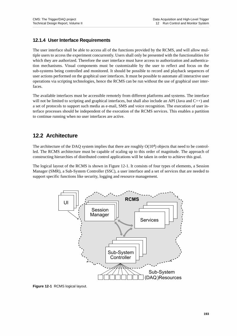
CMS: The Trigger/DAQ project Data Acquisition and High-Level TriggerTechnical Design Report, Volume II 12 Run Control and Monitor System
12.1.4 User Interface Requirements
The user interface shall be able to access all of the functions provided by the RCMS, and will allow mul-tiple users to access the experiment concurrently. Users shall only be presented with the functionalities forwhich they are authorized. Therefore the user interface must have access to authorization and authentica-tion mechanisms. Visual components must be customizable by the user to reflect and focus on thesub-systems being controlled and monitored. It should be possible to record and playback sequences ofuser actions performed on the graphical user interfaces. It must be possible to automate all interactive useroperations via scripting technologies, hence the RCMS can be run without the use of graphical user inter-faces.
The available interfaces must be accessible remotely from different platforms and systems. The interfacewill not be limited to scripting and graphical interfaces, but shall also include an API (Java and C++) anda set of protocols to support such media as e-mail, SMS and voice recognition. The execution of user in-terface processes should be independent of the execution of the RCMS services. This enables a partitionto continue running when no user interfaces are active.
12.2 Architecture
The architecture of the DAQ system implies that there are roughly O(104) objects that need to be control-led. The RCMS architecture must be capable of scaling up to this order of magnitude. The approach ofconstructing hierarchies of distributed control applications will be taken in order to achieve this goal.
The logical layout of the RCMS is shown in Figure 12-1. It consists of four types of elements, a SessionManager (SMR), a Sub-System Controller (SSC), a user interface and a set of services that are needed tosupport specific functions like security, logging and resource management.
Figure 12-1 RCMS logical layout.
UIUI
Session Manager
Services
Sub-SystemController
Sub-System(DAQ)Resources
RCMSUI
193

CMS: The Trigger/DAQ project Data Acquisition and High-Level TriggerTechnical Design Report, Volume II 12 Run Control and Monitor System
The execution of a partition is defined as a “session”. A session is the allocation of all the hardware andsoftware of a CMS partition needed to perform data-taking. Multiple sessions may coexist and operateconcurrently. Each session is associated with a Session Manager (SMR) that coordinates all actions. TheSMR accepts control commands and forwards them through a sub-system controller (SSC) to the compo-nents under its control.
Single commands that are initiated by the user will be interpreted, expanded into sequences of commandswhere applicable, and routed to the proper sub-system resources by different RCMS components. Statusinformation resulting from the actions corresponding to the commands submitted is expected asynchro-nously and is logged and analysed by the RCMS. The RCMS also handles all information concerning theinternal status, malfunctions, errors and, when required, monitor data from the various DAQ subsystems.The sub-systems controlled by the RCMS, corresponding to the main elements of the DAQ are shown inFigure 12-2.
Subsystems are connected for control and monitor purposes via the “DAQ Service Network” (DSN),which is based on switched Ethernet. A subsystem is composed of DAQ resources which are any hard-ware or software components that can be managed directly or indirectly through the DSN. The resourcescurrently defined for the different subsystems are listed in Table 12-1. The DSN can also be used for localdata acquisition.
Figure 12-2 Session Managers and Sub-Systems defined in the RCMS.
Services
EVBCtrl
TRGCtrl
GTPMuCalo
EVB Sub-System TRG Sub-System EVF Sub-System
RCMS Session Manager
UI
Services Connection
FEDBuilder
RUBuilder
EVFCtrl
DCSCtrl
CSCtrl
CS Sub-SystemDCS Sub-System
194

CMS: The Trigger/DAQ project Data Acquisition and High-Level TriggerTechnical Design Report, Volume II 12 Run Control and Monitor System
The block diagram of the RCMS, showing the various services to support interaction with users and tomanage subsystem resources, is shown in Figure 12-3. These services are:
• Security Service (SS). Provides login and user account management functions.
• Resource Service (RS). Provides access to the configuration database (ConfDB) that stores all theinformation about partitions and DAQ resources. The RS also handles the global “alive heart beat”of the CMS DAQ.
• Information and Monitor Service (IMS). Collects messages and monitor data coming from DAQresources or internal RCMS components and stores them in a database (LogDB). The IMS can dis-tribute these messages to any external subscriber, with the possibility of filtering them according toa number of criteria, e.g. the message type, the level of severity and the source of the message. A
Table 12-1 Subsystems and their resources, as defined in the RCMS.
Subsystem Resources defined
Event Builder (EVB) FED Builder, RU Builder (RU, BU and EVM)
Event Filter (EVF) Filter Units
Trigger (TRG) Calorimeter Trigger, Muon Trigger, Global Trigger
Detector Control System (DCS) Values accessible through the SCADA product
Computing Services (CS) Storage, Monitor Services
Figure 12-3 Block diagram of the Run Control and Monitor System.
UserDB
ConfDB
LogDBSession Manager
SecurityService
ResourceService
Info&MonService
Job Ctrl
ProblemSolver
Sub-SystemController
UI
Serv
ice
Con
nect
ion
Sub-System(DAQ )Resources
195
CMS: The Trigger/DAQ project Data Acquisition and High-Level TriggerTechnical Design Report, Volume II 12 Run Control and Monitor System
similar mechanism is also used to distribute monitor data. The IMS also supports logbook facili-ties.
• Job Control (JC). Starts, monitors and stops, when necessary, the software elements of the RCMS,including the data acquisition components.
• Problem Solver (PS). Uses information from the RS and IMS to identify malfunctions and attemptsto provide automatic recovery procedures where applicable.
The above set of services can be distributed over a number of computing nodes for scalability and faulttolerance.
12.3 RCMS and DAQ Operation
The CMS data acquisition system can be operated in one of two ways:
• Partitioned mode, in which one or more DAQ partitions are used (see Section 4.4). All subsystemsare partitioned according to the specific data-taking requirements, e.g. calibration runs, debuggingof a specific subdetector. In this mode, multiple DAQ sessions can run concurrently. A special caseof this mode is a “physics run” in which all operational detectors are used in a single partition. Aphysics run includes all five DAQ elements, namely the trigger, the event builder, the event filtersub-systems, the detector control system and computing services.
• Stand-alone mode, in which the detector partitions work independently using an individual triggerand individual data acquisition system. The stand-alone DAQ uses FED supervisor processors asReadout Units and the DSN for the event builder1. FED supervisor processors will be equippedwith XDAQ software both to control and setup the FEDs and to acquire data when they are work-ing in stand-alone mode. In this case BU and FU functionalities (including event storage capabili-ty) can be embedded in the FED supervisor.
12.3.1 State Definitions and System Synchronization
All RCMS subsystems can handle basic commands like “halt”, “configure”, “enable”, “disable”, “sus-pend” and “resume” that correspond to the state transitions defined for the XDAQ executive (seeSection 11.2.2, "Application Interfaces and State Machines" and Figure 12-4). The responses to the exe-cution of these commands are reported to the IMS. All subsystems implement a state machine similar tothe one in Figure 12-4
Controlling a large number of resources increases the probability of one or more resources failing. Initial-ization and configuration must tolerate these failures if they are related to non-critical components. Thesynchronisation of state changes within a large number of resources also requires an efficient controlmechanism to fulfill timing requirements.
Faults can significantly change run conditions, and therefore their occurrence together with the state tran-sitions of all resources must be recorded. Critical faults will stop the system and raise alarms, whereasnon-critical faults will be tolerated. However a combination of non-critical faults can generate a criticalsystem fault.
1. These are the BDN, BCN and RCN described in Chapter 6, "Event Builder Networks".
196

CMS: The Trigger/DAQ project Data Acquisition and High-Level TriggerTechnical Design Report, Volume II 12 Run Control and Monitor System
12.3.2 Run Definition
A data run is defined as the interval between the starting and stopping of data taking. Traditionally, a newrun was started either because of major changes in run conditions or because of DAQ operations. Runconditions include such information as calibration constants and trigger tables, whereas DAQ resets andtape changes are examples of DAQ operations.
The start of a new run entails a flushing of the event data in the system. This has to be avoided, becausethe buffer sizes and number of components to be controlled in the CMS experiment imply a significantamount of deadtime.
With current database technology, it is possible to continuously record all significant variations in the runconditions that affect the quality of acquired data. This capability no longer necessitates starting a newrun when a significant change in the run conditions occurs, thus reducing the number of times a systemflush has to be performed. Time tags will be used to associate run conditions with event data.
12.3.3 Sessions and Partitions
The subdetectors, such as the muon detectors, tracker and calorimeters, represent “natural” partitionboundaries within the DAQ system. These partitions are reflected in those DAQ sub-systems that have todeal directly with the detectors and their electronics like DCS and the event builder. These physical parti-tions impose constraints on the definition of the logical partitions that will be stored in a database. Thesame is true for the trigger where the partitions are imposed by the TTC distribution topology. However,this is not the case for the event filter where partitions are freely configurable, as they are only influencedby the computing power required by the session to which they belong.
The DCS, from the point of view of the RCMS is an external system with its own independent partitionmanagement. However, during data-taking, the RCMS instructs the DCS to set up and monitor partitionscorresponding to the detector elements needed for the data-taking run in question. The RCMS also has ac-cess to all partition information in the DCS.
Before a partition can be used it must be validated. It is invalid if it does not include a complete and con-sistent set of elements needed for a DAQ run. The completeness and consistency check depends on thesub-system for which the partition is defined. Taking an event builder as an example, the check includes
Figure 12-4 State diagram of a generic DAQ component.
Halt
Failed
Ready
Suspended
EnabledConfigure
Halt
Disable
Enable
SuspendHalt
Fail
Resume
197

CMS: The Trigger/DAQ project Data Acquisition and High-Level TriggerTechnical Design Report, Volume II 12 Run Control and Monitor System
the verification that at least one RU, one BU and one EVM are included. A valid partition is activated byallocating physical sub-system resources to it. The activation can fail if the partition tries to use unavaila-ble resources. The activation of a partition corresponds to the creation of a session ready to accept com-mands. A running session can be joined by several user interfaces.
12.3.4 Interface to DCS
The RCMS instructs the Detector Control System (DCS) to act according to the specific needs of a da-ta-taking session. At all other times, the DCS runs in stand-alone mode. The DCS, as described inChapter 13, "Detector Control System", can be accessed through a specific XDAQ application (seeSection 11.2.6.2, "Common Application Components").
12.4 Design of the RCMS Components
This section describes the design of all RCMS components. For each component an API (C++, Java) hasbeen defined and is described in [12-1].
12.4.1 Session Manager (SMR)
The SMR is created to coordinate a session by the RS when that session is opened. The RS also providesthe SMR, at the time of its creation, with all the needed information concerning the subsystems and thecomposition of the partitions making the session. The lifetime of the SMR corresponds to the lifetime ofthe session and it is deleted when the session is closed. Once the session is opened, it can be joined byseveral users. The SMR coordinates user access to the session and propagates commands from the usersto the SubSystem Controllers (SSCs) which belong to the session. Figure 12-5 shows a typical interactiondiagram where a command is issued from a user interface that has already joined a session. The exampleshown in the figure includes two SSCs (A and B). In this case SSCs inform the Information and MonitorSystem (IMS) of the status change of the subsystems they control. The diagram also shows a system statedisplay that retrieves, at regular time intervals, the global status of the system.
Figure 12-5 SMR interaction with the other RCMS components.
UI SMR SSCA SSCB IMS SSD
cmd_Stat
cmd (pars)
User Interface SessionManager
Sub-SystemController-A
Sub-SystemController-B
InformationMonitor Srvc
System StateDisplay
get_Status
Status
get_Status
Status
cmd_SSCA
cmd_Stat_AStat_A
cmd_SSCB
cmd_Stat_BStat_B
198

CMS: The Trigger/DAQ project Data Acquisition and High-Level TriggerTechnical Design Report, Volume II 12 Run Control and Monitor System
12.4.2 Security Service (SS)
This service provides the RCMS login facilities for user authentication and authorization, providing dataencryption when demanded. The SS manages a database (UserDB) that stores profiles for each user in-cluding access rights and a personalized work history, e.g. open sessions and defined partitions. The SSkeeps track of the user context such as the connection and client interface type (browser, stand-alone ap-plication, etc.).
12.4.3 Resource Service (RS)
This service handles all the resources of the DAQ system through partitions and their sessions. Resourcescan be discovered, allocated and queried. A resource can be any hardware or software component that canbe managed directly or indirectly through the DAQ service network. Figure 12-6 shows the block dia-gram of the Resource Service.
In accordance with the requirements, partitions can only use “available” resources whose state (runningor down) is verified when the partition is activated for data-taking. It is the responsibility of the ResourceService to check for resource contention with other active partitions. The RS must also signal temporaryunavailability when activating the partition.
A periodic scan of all the required registered resources, the “alive heartbeat”, will keep the database ofavailable resources up to date. Two types of scan are foreseen:
• ping scan: Checks if resources are reachable, and is expected to take a time of O(s)
• status inquiry: the status is retrieved and then dispatched to the IMS, described in the followingsection. This type of scan is expected to take a time of O(minutes)
Figure 12-6 Block diagram of the Resource Service.
ResourceSubscribing
Handler
Still aliveheartbeat
Session,Partition
management
Available
Con
figur
atio
n D
ataB
ase
Resources
PartitionDatabase
SoftwareDatabase
New Node subscribe request
Ping all the registered nodes enquire status of all the activated resources
SessionsPartitionsdefinition
Session,Partition Setup
ManualResources
Handler
WEB applications
199

CMS: The Trigger/DAQ project Data Acquisition and High-Level TriggerTechnical Design Report, Volume II 12 Run Control and Monitor System
12.4.4 Information and Monitor Service (IMS)
This service is responsible for collecting information from all subsystems in the DAQ. Figure 12-7 showsthe block diagram of the IMS.
There are several types of messages collected from the subsystems that are catalogued according to theirseverity level and type such as: informational, monitoring, warning and errors. Data can be provided innumeric formats, histograms, tables and other constructs.
Each record of information sent to the IMS contains the following items:
• time stamp: when the message/monitor information was generated
• message identification
• the source of the information, uniquely identified by the session, sub-system, partition, softwareapplication and hardware board
• information type: informational, monitoring, warning and error
• specific fields according to the information type
The time stamp facilitates tracking of different events, as well as correlating them. All resources are syn-chronized with time servers providing a global time accuracy of O(ms).
The IMS collects and organizes the incoming information in an internal database and publishes it to theIMS subscribers. Subscribers can register for specific messages that can be selected on the basis of the in-formation source, the error severity level, the type of messages or a combination of these tags. The IMSalso monitors event data providing permanent recording and snapshot buffers for subscribers. Any infor-mation can also be retrieved by a client via simple query procedures.
Figure 12-7 Block diagram of the Information and Monitor Service.
MessageLogger (DB)
State Logger
Monitor-HistoryDatabase
Clie
ntSu
bscr
iber
Mes
sage
Filte
r and
Subs
crib
er
MonitorSystems
AlarmDisplay
SystemStatusDisplay
ErrorStatistics
Message (Error, Warning, .. )
Resource Status Change
Monitor Info
WEB applications
200

CMS: The Trigger/DAQ project Data Acquisition and High-Level TriggerTechnical Design Report, Volume II 12 Run Control and Monitor System
The IMS is also responsible for storing and maintaining the run logbook. This type of information is man-aged by the Session Manager that uses the IMS back-end facility to store them.
12.4.5 Job Control (JC)
Job Control is a utility that allows the remote execution and supervision of processes as outlined inSection 16.6.1, "Cluster Management". This tool is necessary to start, monitor and stop, when needed, thesoftware infrastructure of the RCMS on the main management nodes and subsystem resources., i.e. thevarious managers and the databases.
12.4.6 Problem Solver (PS)
The Problem Solver (PS) is a central service of the RCMS with the main task of collecting alarms fromthe DAQ system and potentially determining recovery procedures. Figure 12-8 shows the block diagramof the PS.
The PS subscribes to the IMS to receive the information it requires from the DAQ components it is inter-ested in. This information is processed by a correlation engine and the result is used to determine a poten-tial recovery action. When the PS cannot determine such an automatic recovery procedure, it simplyinforms the system operator, providing any analysis results the PS may have obtained.
The PS must interact with the asynchronous Trigger-Throttling System (aTTS, see Section 5.2.3) to pro-vide the back-pressure signal to the trigger to block data taking while the DAQ system recovers from fail-ures. This may be used to allow the detachment from the DAQ chain of a given component, e.g. a
Figure 12-8 Block diagram for the Problem Solver.
Information Monitor System
(IMS)
OperatorIntervention
SessionManager
aTTS(asynchronous Trigger and Throttle System)
Prob
lem
Sol
ver Correlation
Engine
ActionBuilder
201

CMS: The Trigger/DAQ project Data Acquisition and High-Level TriggerTechnical Design Report, Volume II 12 Run Control and Monitor System
Readout Unit or a Builder Unit, and to reconfigure the system. Other faults (e.g. a misalignment of theevent fragments read out of the FEDs) could involve a reset of the front-end electronics, which impliesthat access to the fast reset signal is necessary.
Automatic recovery procedures are communicated to the Session Manager that controls the component inquestion. The procedures vary from controlling single DAQ components to the entire system.
12.4.7 Sub-System Controller (SSC)
An SSC, as shown in Figure 12-9, consists of a Function Manager (FM) and a local database (DB) serv-ice. There is one FM per partition that receives requests from an SMR and transforms them into the corre-sponding requests for actions that are sent to the subsystem. Since partitions can be nested, the SSC canbe organized in a hierarchical manner.
A hierarchy can map to a corresponding physical architecture, with a shared load among different proces-sors. An example of this is shown in Figure 12-10. The local database (DB) service can be used as aproxy to the RS and IMS to facilitate software and configuration download and monitoring.
12.5 Software Technologies
Web technologies and related developments play a fundamental role in the implementation of the pro-posed design. In this section we review some of the present trends that have been followed.
12.5.1 Web Technologies
Web technologies and in particular Web Services have been chosen because they have been designed tointerconnect highly heterogeneous and distributed systems, therefore implying a rich choice of availabletools and solutions. Among the available technologies, the XML data format and the W3C standardSOAP protocol have been adopted (see Section 11.2.5, "Protocols and Data Formats") as the main meansfor communication. For more information about these and their associated tools see Section 11.2.2, "Ap-plication Interfaces and State Machines".
Figure 12-9 Block diagram of a SubSystem Controller.
FM(session i)
DBService
Sub-SystemResources
Sub-System Controller (SSC)
202

CMS: The Trigger/DAQ project Data Acquisition and High-Level TriggerTechnical Design Report, Volume II 12 Run Control and Monitor System
12.5.2 Security
Security issues are crucial for a system such as the RCMS that has clients distributed around the globe. Aweakness in security can have serious consequences on the correct operation of the system. Security is aproblem in its own right and the RCMS has therefore chosen to leverage existing solutions in the scope ofwidely distributed systems. The Grid Security Infrastructure (GSI) of the Grid Forum has submitted anInternet Draft [12-2] which provides some preliminary guidelines to GRID infrastructures. This is a po-tential candidate to address the security needs of RCMS, because it has been proposed for the security in-frastructure of the LHC Computing Grid (LCG) project [12-3].
12.5.3 Database
Databases will be used by the RCMS to handle different types of information, ranging from hardware andsoftware configurations to user identification parameters and system book keeping information. Relation-al database management systems are appropriate for this task and furthermore guarantee the required lev-el of robustness and scalability. It should be noted however that native XML database technologies existand are being investigated because they remove the need to transform between XML data and relation ta-ble structures. For more information about the chosen technologies see Section 11.3.3, "Software Devel-opment Environment".
12.5.4 Expert Systems
As described in Section 12.4.6, "Problem Solver (PS)", the PS is a central service of the RCMS. Its maintask is to correlate different types of input information (errors, warnings, messages, etc.) to identify globalerror conditions in the DAQ system and to propose, wherever possible, appropriate recovery actions. ThePS can be implemented by conventional procedural languages, however artificial intelligence techniqueslike rule-based expert systems permit modelling at a higher level of abstraction, thus allowing the formu-lation of problems in almost human terms. Commercial [12-4] and public-domain [12-5] expert systems
Figure 12-10 Structure of a generic sub-system.
Sub-System Controller
DAQ resource
203

CMS: The Trigger/DAQ project Data Acquisition and High-Level TriggerTechnical Design Report, Volume II 12 Run Control and Monitor System
exist. For example, Jess [12-6] could be easily integrated into the current Java-based infrastructure, and iscurrently being evaluated.
12.6 RCMS Prototypes
Prototypes have been developed to provide proof of principle for the proposed RCMS design and thetechnologies it uses. A prototype has been implemented for the small DAQ systems used for experimentproduction and the test beams. Two prototypes addressing specific functions, hereafter referred to as dem-onstrators, have also been developed to study scalability issues. Medium scale O(100) test-bed systemsare used in this case to emulate parts of the hierarchical structure of the final DAQ system.
12.6.1 RCMS for Small DAQ Systems
A prototype RCMS system has been developed for test beam setups, and the detector validation, triggerand front-end electronics test-benches. The system is based on the XDAQ framework as described inChapter 11 and implements all services shown in Figure 12-3 with the exception of the “Problem Solver”.Multiple sessions can run concurrently. DB proxies and management systems are not implemented in thesub-system controllers, due to the small number of nodes. The Job Control service (JC) is also not used,since XDAQ executives were started automatically at boot time. The following paragraphs give a brief re-port on the design and tools used to implement the prototype. A full description of the system can befound in [12-7].
The services and managers have been implemented as a collection of Java servlets using the ApacheTomcat platform. Figure 12-11 displays a graphical representation of the system when a single Tomcat[12-8] is used. SOAP messages are used as the primary communication mechanism. Relational (MySQL)and native XML (XML:DB [12-9]) database technologies have been exercised for persistent storage.Figure 12-12 shows the implementation of the Resource Service. The Castor [12-10] tool has been usedto map XML data structures to Java class definitions.
The session and function managers incorporate a Finite State Machine (FSM) to track the status of thecorresponding components. The FSM is defined by an XML document and actions are declared throughJava classes. Both definition and implementation are managed by the Resource Service (RS). When a ses-sion is opened, the RS launches the session and function managers, passing them the corresponding statemachine definitions along with the Java code as well as the information about the hardware and softwareconfiguration.
The described system has been integrated into the data acquisition system that is used to validate muonchambers for the CMS detector at the Legnaro production center and at the CERN storage area. A similarsystem is also used for the chamber tests with muon beams in the H2 area and at the Gamma IrradiationFacility at CERN.
12.6.2 RCMS Demonstrators
Two demonstrators have been set up to prove the scalability of the RCMS architecture and the technolo-gies it uses.
The first demonstrator uses the basic elements of the prototype RCMS system developed for small DAQsystems, to explore the ability to command a set of DAQ nodes running XDAQ executives. Both flat and
204

CMS: The Trigger/DAQ project Data Acquisition and High-Level TriggerTechnical Design Report, Volume II 12 Run Control and Monitor System
hierarchical network topologies are used to prove that the RCMS fits the requirements of a distributedsystem with the size foreseen for CMS. A 120 node PC cluster, corresponding to the size of a full readoutunit builder, has been set up with a single RCMS host. All PCs are 1 GHz Pentium-III dual-processor ma-chines. The XDAQ executives perform dummy actions, merely implementing a state change acknowl-edge when a command is received. The time measured in the tests therefore represents the time requiredto perform a state change of the entire cluster. Figure 12-13 shows the measured time as a function of thenumber of nodes addressed. Line A represents the behaviour when the function manager works sequen-tially, sending a command and waiting for an acknowledgement before sending the next command to an-other node. Line B shows a multi-threaded implementation where multiple nodes are sent commandsconcurrently. In this case a command can be sent to all nodes within 150 ms. Further optimization can beperformed through a hierarchical configuration as shown in Figure 12-14. Intermediate nodes with FMfunctionality are controlled by the master node, to relay the commands to the leaf nodes. Line C inFigure 12-13 shows the performance of this approach (as in Figure 12-14) with two intermediate nodes,each one controlling 64 leaf nodes.
Figure 12-11 Block diagram of the RCMS prototype.
Figure 12-12 Block diagram of the Resource Service Prototype.
UserDB
ConfDB
LogDBSession Manager
RCMSServlet ContainerAphace Tomcat
SecurityService
ResourceService
Info&MonService
InternetXML-http
Job Ctrl
FSMXDAQ adapter
ProblemSolver
Sub-SystemController
UI
Serv
ice
Con
nect
ion
Sub-System(DAQ)Resources
FSM
XML:DB+mySQL
JAVA Objs
JAVA servlet
Resource ServiceServlet container (TOMCAT)
XML DBXML
http
REL DB
XML Parser(CASTOR)
XML Parser(CASTOR)
JAVA Client
XML ParserC++Client
XML ParserhtmlClient
205

CMS: The Trigger/DAQ project Data Acquisition and High-Level TriggerTechnical Design Report, Volume II 12 Run Control and Monitor System
The second demonstrator is a simplified version of a log message service based on Web Service technolo-gy. The PCs used for deployment were from the same cluster as the first demonstrator. Multiple instancesof the service hosted by different physical machines have been implemented to show scalability. Every in-stance exports a logging interface through the Web Service Description Language (WSDL) [12-11]. Thisinformation is then published using Universal Description, Discovery and Integration (UDDI) registries[12-12] located in a dedicated host. Clients looking for the log services, query first the UDDI server todiscover the location of the service and retrieve the access method. Up to 4 web services and a fixed set of15 clients have been used. The Web Service infrastructure, including the UDDI registry, has been devel-oped using the Glue platform [12-13]. The performance of the logging service scales linearly with thenumber of instances of the service available (Figure 12-15).
The second demonstrator shows the following advantages of Web Service technologies:
• rapid application deployment
• run-time configurability and maintenance through the addition or the removal of services viaUDDI
Figure 12-13 Time spent to send a command to the PC cluster vs. the number of nodes of the cluster.
Figure 12-14 PC nodes organized in a hierarchical architecture with an intermediate layer.
Tim
e [m
s]
Number of Nodes0
050 100
100
200
300
Sequential FMIFM with Threads2 intermediate FMs
A
B
C
Function Manager
DAQ resource
Interm.FM
Interm.FM
RootFM
Interm.FM
206

CMS: The Trigger/DAQ project Data Acquisition and High-Level TriggerTechnical Design Report, Volume II 12 Run Control and Monitor System
• standardization of service descriptions and access
12.7 Summary and Outlook
In this chapter the design and architecture of the RCMS have been presented. A service driven architec-ture has been adopted due to its intrinsic modularity and scalability. This approach leads to a design whichcan exploit the modern concept of world-wide interoperable services found in existing Web technologies.
Prototypes and demonstrators have been developed using state-of-the-art technologies to provide a proofof principle of the proposed approach. However, some products such as XML databases and Web Serviceplatforms are very recent and require further investigation into their stability and robustness.
The prototypes developed did not attempt to test the scalability of the database technologies used. How-ever, different approaches to cope with scalability requirements exist and have to be validated in the scopeof the RCMS system.
Distributed architectures, like the one proposed, are intrinsically weak in terms of security. This requiresfurther investigation, for example the tracking of other projects (e.g. LCG) based on large distributed sys-tems.
Recent trends in Grid technology like the Open Grid Service Architecture (OGSA) [12-14] demonstratethe interest in extending distributed computing to include Web services and related technologies. Theadoption of OGSA could have positive effects on the design, deployment and maintenance of the system.Profit can be made from synergies with other OGSA based projects. Thus the present OGSA implementa-tion is currently being evaluated for the RCMS.
Some of the RCMS functionalities have been tested in the context of small DAQ systems used for testbeam setups and detector validation. This activity will continue in the future and will be extended totest-benches for the trigger and electronic Front-ends. At present, the setups for the drift tube muon cham-
Figure 12-15 Performance of the Log Service in function of the number of servers are providing the service
0
500
1000
1500
2000
2500
3000
3500
1 2 3 4Number of Web Services
Tota
l No.
of m
essa
ges/
s (re
ceiv
ed b
y th
e se
rvic
es)
207

CMS: The Trigger/DAQ project Data Acquisition and High-Level TriggerTechnical Design Report, Volume II 12 Run Control and Monitor System
bers are driven by the RCMS, while the integration work is in progress both for the tracker and DAQ-col-umn.
The presented prototypes show that a system based on distributed services that are interconnected byopen and standard protocols and have the ability to export their service interfaces, has the modularity andscalability required to configure, control and monitor a CMS DAQ segment (128 nodes). This result is en-couraging because modular systems, in terms of FED and RU Builders, map well to the scale of the actualsystem to be implemented.
The transition from the prototype phase of the RCMS to the final implementation, which requires focus-ing on software robustness and adherence to production quality rules, will be an important effort in thefollowing years.
12.8 References
12-1 RCMS API documentation can be found at http://RCMS.lnl.infn.it/doc/index.html
12-2 I. Foster et al., “A Security Architecture for Computational Grids”, in Proceedings of the 5th ACM Conference om Computer and Communications Security, 1998
12-3 The LHC Computing Grid (LCG) Project, http://lcg.web.cern.ch/LCG/
12-4 Blaze Advisor,http://www.blazesoft.com
12-5 CLIPS, A tool to build expert systems, http://www.ghg.net/clips/CLIPS.html
12-6 Jess, The rule engine for Java platform, http://herzberg.ca.sandia.gov/jess/
12-7 L. Berti et al.,” Run Control and Monitor System for the CMS Experiment”, LNL-INFN(Rep), 2002, to be published.
12-8 The Jakarta Project: Apache Tomcat, http://jakarta.apache.org/tomcat/
12-9 XML:DB database, see http://www.xmldb.org/
12-10 The Castor Project, http://castor.exolab.org/
12-11 Web Service Definition Language, http://www.w3.org/TR/wsdl
12-12 Universal Description, Discovery and Integration (UDDI) project, http://www.uddi.org/
12-13 GLUE, a Java Web Service Platform, http://www.themindelectric.com/
12-14 I. Foster et al., ”The Physiology of the GRID”, http://www.globus.org/research/papers/ogsa.pdf
208

CMS: The Trigger/DAQ project Data Acquisition and High-Level TriggerTechnical Design Report, Volume II 13 Detector Control System
13 Detector Control System
The main aim of the Detector Control System (DCS) is to ensure the correct operation of the CMS exper-iment, so that the data taken with the apparatus is of high quality. The scope of the Detector Control Sys-tem (DCS) is therefore very wide and includes all subsystems and other individual elements involved inthe control and monitor of the detector, its active elements, the electronics on and off the detector, the ex-perimental hall as well as communications with the accelerator. The DCS also plays a major role in theprotection of the experiment from any adverse events. Many of the functions provided by DCS are neededat all times, and as a result selected parts of the DCS must function continually on a 24-hour basis duringthe entire year.
13.1 Introduction
The primary function of the DCS [13-1] will be the overall control of the detector status and its environ-ment. In addition DCS has to communicate with external entities, in particular the RCMS and the acceler-ator.The integration of the DCS system into the overall online system is illustrated in Figure 13-1. The
DCS will be a slave to the Run Control and Monitor System which will be in charge of the overall controland monitoring of the data-taking process. When the DCS will operate outside data-taking periods it willact as the master of the active detector components and other parts of the system. The major tasks in thisset will be:
• central supervision of all DCS elements,
Figure 13-1 Integration of DCS in the online system.
Services
DCS TRG CSCtrl Ctrl Ctrl
GTPMuCaloRUFEDFEC
EVB Sub-System TRG Sub-System EVF Sub-System
Session Manager
UI
Services Connection
Run Control and Monitor System (RCMS)
DCS/DSS subsystems
Pixel Tracker ECAL HCAL CSC DTInfrastructure RPC
DCS supervisorCentralServices
Data/Calibration Archive Configuration Run ConditionsApparatus History
DatabasesCS Sub-Systems
EVBCtrl
EVFCtrl
209

CMS: The Trigger/DAQ project Data Acquisition and High-Level TriggerTechnical Design Report, Volume II 13 Detector Control System
• communication with external systems (RCMS, accelerator),
• user interfaces, and
• bookkeeping of detector parameters and used DCS hardware/software components.
An integral aspect of the DCS is its provisions for three important safety-related functions, namely
• Detector security (DCS/DSS)
• Alarm handling (DCS)
• Software access control (DCS)
The highest level of safety, “Level 3”, is established for the most severe situations where a human lifemay be at threat. This critical level will be handled by the CERN Safety Alarm Monitoring (CSAM)[13-2]. Less severe alarms, referred to as “Level 1” and “Level 2”, will be handled either by the DetectorSafety System (DSS) [13-3] or by the DCS system itself. The exact boundary between the two will be de-fined in the future.
Another major task of the DCS is the control and monitoring of the systems regulating the environment atand near the experiment, a set of tasks traditionally referred to as “Slow Controls”, and which include,among others:
• Handling the supply of electricity1 to the detector,
• Other DCS-related detector electronics (e.g. calibration systems),
• Control of the cooling facilities and the overall environment near the CMS subdetectors,
• Supervision of all gas and fluids subsystems,
• Control of all racks and crates
13.2 Requirements
This section discusses the main requirements on the DCS. It is not meant to be exhaustive, in the sensethat it is sufficient to obtain an engineering blueprint for the system. Rather, the discussion highlightssome of the major challenges that the system has to address, leaving more standard requirements, e.g. likethe programmability of the system, to the actual implementation, under the assumption that such second-ary requirements are well understood through work on previous High Energy Physics experiments.
13.2.1 General System Requirements
The major system-wide requirements on the CMS DCS are:
• Most importantly, the system has to be reliable: this requires safe power, redundancy and reliablehardware in numerous places.
• The system must be modular and hierarchical.
1. This task is usually referred to as “High and Low Voltage Control”.
210

CMS: The Trigger/DAQ project Data Acquisition and High-Level TriggerTechnical Design Report, Volume II 13 Detector Control System
• It has to be partitionable in order to allow independent control of individual subdetectors or partsof subdetectors. Conversely, integration of different parts into the global system must be possiblewith ease.
• The system needs automation features in order to speed up the execution of commonly executedactions and also to avoid mostly human mistakes in such repetitive actions.
• The system has to be easy to operate: a few non experts should be able to control the routine oper-ations of the experiment.
• The system must be scalable: it must be possible to integrate new subdetectors or subdetector parts.
• The system must provide generic interfaces to other systems, e.g. the accelerator, the CMS RunControl and Monitor system.
• The system must be easy to maintain. This requirement strongly favours the usage of commercialhardware and software components.
• The system has to be homogeneous, which will greatly facilitate its integration, maintenance andpossible upgrades, and has to have a uniform “look and feel” throughout all of its parts.
• The system has to provide a possibility for remote control via the internet to allow non CERN res-ident detector groups to do maintenance and control from their home station.
Beyond these general system-wide requirements there are a few additional ones resulting from the specif-ic design and implementation of the various CMS subdetectors. These requirements are the subject of thefollowing section.
13.2.2 Subdetector Requirements
The Detector Control Systems of individual subdetectors will be connected to the central DCS supervisorhierarchy. These systems will handle all the individual detector electronics which are only partially basedon standard components like, for instance, the CAEN high-voltage power supplies. The low-voltage sys-tem as well as the gas system will be common for all sub-detectors, whereas the cooling systems will builtindividually by each sub-detector. For the front-end control links, the major part of the sub detectors hasadopted the solution developed for the CMS tracker (CCU). Figure 13-2 illustrates the current situationfor the front-end control links. A summary of the DCS items to be controlled in each sub detector is givenin Table 13-1. Some particularities of the different sub-detectors are sketched in the following paragraphs.
13.2.2.1 Magnet
The magnet will be an independent system communicating with the central DCS supervisor. The controlof this system will be carried out by a dedicated group responsible for the magnet as a whole. The centralDCS will only receive status information from the magnet which will thus appear as a sub-detector whichdoes not accept commands but only provides status information.
13.2.2.2 Tracker
Stringent requirements in the tracker system arise from the required cooling. To maintain the tracker with-in its working temperature, a reliable controls system built of Programmable Logic Controllers (PLC) willbe installed. Although this system is part of the DCS, it will work independently and will only report its
211

CMS: The Trigger/DAQ project Data Acquisition and High-Level TriggerTechnical Design Report, Volume II 13 Detector Control System
status to the DCS system. It will be possible for this to take direct emergency actions (e.g. switch off thepower supplies) hard-wired connections.
An important element of the tracker control system is the link to the front-end electronics control [13-4],which uses a network similar to the IBM token-ring. The Front-End Controller (FEC) which will behoused in a VME crate in the counting room is the master on the ring and the Communication and Control
Figure 13-2 Implementation of the control links for the front-end electronics.
Table 13-1 Summary of DCS tasks, broken down into those that are common across sub-systems and thosethat are specific to each sub-detector.
Detector Common Specific
Pixel tracker HV, LV, gas, FE links (CCU) Cooling, temperature monitoring
Strip tracker HV, LV, gas, FE links (CCU) Cooling, temperature monitoring, thermal screen, alignment
ECAL HV, LV, gas, FE links (CCU) Cooling, temperature monitoring, laser
HCAL LV HV, radioactive source, laser, LEDs, FE links, cooling, temperature monitoring
DTs HV, LV, gas, cooling, temperature monitoring Alignment, FE links, cooling
CSCs HV, LV, gas FE links, alignment
RPCs HV, LV, gas, FE links (CCU), cooling, tem-perature monitoring
RS 422
RS/RS Hub
Pixel Tracker ECALPreShower
HCAL µDT µRPC µCSC L1-Trigger DAQ
FES param.LV, I, T, I2C, Clock, LV1
FES param.LV ,ClockLaser, LED
FES param.LV, I, T, I2CClock, LV1
FES param.LV, I, T, I2CClock, LV1
CCUDCU
MiniCrate
MiniCrate
Eth/RS 485
HV
140�RBX140 �MM
250� Rings2500�CCU20000 � DCU
500� Rings40000�CCU/DCU
RS/RS Hub
10� RS485 rings250�RS232 links250�Minicrates
3 Systems40 Crates800 FPGA boards
8 Systems2000 PCs/NICs105 Jobs
RBXCCM
MM
LinkBoard
LinkBoard
VME
VME
VME
DynatemCPU
80 CCU/DDU
232 to 485 Eth. Hub
FECVME10
FECPCI200
FECVME200
FECPC-PCI
6?
FECPC-PCI
6?
FECPC-PCI
6?
FECPC6?
PC-VME PC-PCI
40 M
bit/s
80
links
(dup
lex)
�
40 M
bit/s
250
link
s (d
uple
x)�
I2C
rin
g
I2C
ring
I2C
ring
RS4
85 ri
ng
40 M
bit/s
500
link
s (d
uple
x)�
Eth
erne
t
RS
232
�10
links
RS
485
(10)
RS
422
RS
422
RS
232
�240
link
s
Eth
erne
t
Ethe
rnet
40 M
bit/s
6 li
nks
(dup
lex)
�
FES param.DAQ-FPGALV, I, T?
FES param.Link-FPGALV, I, T?
TTCTTC
TTC
TTC
TTC
TTC
TTC TTC
TTC
TTC
TTC
Acronyms:ECAL�HCALRPCCSCDTTTCFECFESI2CCCUDCU
Electromagnetic CalorimeterHadron CalorimeterResistive Plate ChambersCathode Strip ChamberDrift TubeTiming, Trigger and ControlFrontEnd ControllerFrontEnd SystemsInter-Integrated CircuitCommunication and Control UnitDetector Control Unit
212

CMS: The Trigger/DAQ project Data Acquisition and High-Level TriggerTechnical Design Report, Volume II 13 Detector Control System
Units (CCU) in the front-end electronics on the detector are the slaves. With its two redundant networklines and 40Mb/s transmission speed, the link offers a fail-safe solution with high throughput. Due tothose advantages and its open architecture it will be used, after slight adaptations, by other detectors aswell.
13.2.2.3 Electromagnetic Calorimeter (ECAL)
The ECAL requirements on the cooling system are also very stringent: its temperature has to be kept sta-ble within 0.1o. For this reason, the ECAL will have three sets of temperature probes. Many thousands oftemperature probes will provide a fine-grained temperature map which will be used for corrections to thedata. At present, it is foreseen to transmit these temperature readings via the normal data acquisition path.Coarse-grained temperature information will be sent via the control links and will be used for the supervi-sion of the cooling system. A third group of temperature probes will be used for automatic, hard-wired ac-tion in the event of a failure in the cooling system. The links for the front-end electronics control will bethe same as the ones for the tracker.
13.2.2.4 Hadronic Calorimeter (HCAL)
The amount of data relevant to the control of the HCAL is relatively small. However, a system for passinga radioactive source through the detector will have to be controlled as well as a laser system for calibra-tion.
13.2.2.5 Muon Systems (MUON)
The alignment system will be part of the Muon system (see Section 13.5.4 for further details). Pieces ofthe barrel alignment system will be mounted on the barrel muon chambers and the alignment control willuse the controls links of the barrel muon system. Those links will therefore handle not only the data of thetwo systems, but also the ownership of the controls of the two systems.
13.3 Architecture and Framework
A commercial SCADA (Supervisory Controls And Data Acquisition) system PVSS II [13-5] has beenchosen by all LHC experiments as the supervisory system of the corresponding DCS systems. PVSS II isa development environment for a SCADA system which offers many of the basic functionalities neededto fulfill the tasks mentioned above. PVSS II components for use by all LHC experiments are either al-ready developed and maintained, or are currently under development centrally within the framework ofthe CERN-wide “Joint COntrols Project”, JCOP. The framework provides the tools to build a partitiona-ble controls hierarchy as well as the PVSS II implementation of certain hardware devices.
13.3.1 Command Hierarchy
Detector controls will be organized in a hierarchy as shown schematically in Figure 13-3. The implemen-tation of this organisation will be made purely in software and only represents the logical structure of thedetector. A prototype of the hierarchy mechanism is already implemented in the JCOP framework. Theinterfaces of all nodes in this hierarchy are made such that each node can be connected to any other node.
213

CMS: The Trigger/DAQ project Data Acquisition and High-Level TriggerTechnical Design Report, Volume II 13 Detector Control System
Therefore each node can be placed anywhere in the hierarchy. This allows for independent developmentof the sub-detector systems while it will greatly facilitate their integration into the full system.
The DCS supervisor, at the topmost point of the hierarchy, offers global commands like “start” and “stop”for the entire detector. The commands are propagated towards the lower levels of the hierarchy, where thedifferent levels interpret the commands received and translate them into the corresponding commandsspecific to the system they represent. As an example, a global “start” command is translated into a “HVramp up” command for a sub detector. Correspondingly, the states of the lower levels are summarised bythe upper levels and thus define the state of the upper levels. As an example, the state “HV on” of a sub-detector is summarized as “running” in the global state. The propagation of commands ends at the lowestlevel at the “devices” which are representations of the actual hardware. The SCADA system ensures thatevery action on the devices is transmitted to the hardware and that the state of the devices represent thehardware status. Several possible ways for carrying this out are described in Section 13.4.
13.3.2 Partitioning
The ability to partition the command hierarchy is essential for a detector like CMS which comprises alarge number of subdetector elements. Partitioning implies that a sub tree is cut off from the command hi-erarchy. In this way components can be operated independently from the rest of the tree thus rendering theoperation of the corresponding subdetectors independent of the rest of the system. This mode of operationwill be used mainly for maintenance, calibration, system testing and trouble shooting. Under normal oper-ating conditions, i.e. during a “physics run”, there will be only one partition, comprising all subdetectorsparticipating in the data-taking.
The mechanism of partitioning is illustrated in Figure 13-4. Partitioning is introduced into the commandhierarchy by declaring a node as partitionable. This adds three parameters to each node that provide the
Figure 13-3 Illustration of command hierarchies in the DCS. Commands flow downwards, status flowsupwards.
Supervisor
Control Unit Control Unit
Control Unit
Control Unit
Control Unit
Control Unit
Control Unit
Control Unit Control Unit
Device UnitDevice Unit Device Unit
Device Unit
Device UnitDevice Unit
Detector A
Detector B
Statu
sCom
mands
214
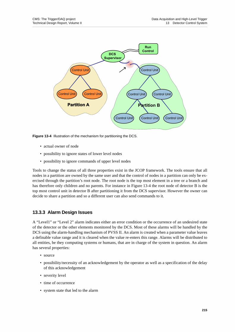
CMS: The Trigger/DAQ project Data Acquisition and High-Level TriggerTechnical Design Report, Volume II 13 Detector Control System
• actual owner of node
• possibility to ignore states of lower level nodes
• possibility to ignore commands of upper level nodes
Tools to change the status of all three properties exist in the JCOP framework. The tools ensure that allnodes in a partition are owned by the same user and that the control of nodes in a partition can only be ex-ercised through the partition’s root node. The root node is the top most element in a tree or a branch andhas therefore only children and no parents. For instance in Figure 13-4 the root node of detector B is thetop most control unit in detector B after partitioning it from the DCS supervisor. However the owner candecide to share a partition and so a different user can also send commands to it.
13.3.3 Alarm Design Issues
A “Level1” or “Level 2” alarm indicates either an error condition or the occurrence of an undesired stateof the detector or the other elements monitored by the DCS. Most of these alarms will be handled by theDCS using the alarm-handling mechanism of PVSS II. An alarm is created when a parameter value leavesa definable value range and it is cleared when the value re-enters this range. Alarms will be distributed toall entities, be they computing systems or humans, that are in charge of the system in question. An alarmhas several properties:
• source
• possibility/necessity of an acknowledgement by the operator as well as a specification of the delayof this acknowledgement
• severity level
• time of occurrence
• system state that led to the alarm
Figure 13-4 Illustration of the mechanism for partitioning the DCS.
DCS Supervisor
Control Unit Control Unit
Control Unit Control Unit Control Unit Control Unit
Control Unit Control Unit Control Unit
Partition BPartition A
RunControl
215
CMS: The Trigger/DAQ project Data Acquisition and High-Level TriggerTechnical Design Report, Volume II 13 Detector Control System
• additional details like a help text describing the alarm and a potential reaction or even cure
Alarms will be logged persistently in the PVSS II database. PVSS II tools, which include a graphical dis-play for active and archived alarms, can be used to browse this database.
13.3.4 Software Access Control
CMS will use communication techniques based on the Internet to offer remote maintenance and surveil-lance of the detector cavern and all its counting rooms. This implies a security risk. An access controlmechanism must be put in place in order to prevent any damage or other disturbance caused by such inci-dents. The DCS system will utilize standard encryption and authentication techniques. On the other handaccess control will be needed to allow for certain actions depending on the expertise of the user. For in-stance an experimenter on shift might only be allowed to switch a detector on or off, while an expertmight be allowed to also change various key voltage settings.
PVSS II offers an intrinsic access mechanism where actions can be restricted on a per-user basis. Howev-er, more sophisticated access mechanisms may eventually be required and therefore, in the scope of theJCOP framework, an extension to the current access control system is planned. A future version of PVSSII, which will provide a simple, web-like remote access is expected to also include access control, encryp-tion and authentication.
13.3.5 Configuration
Many DCS front-end components and their power supplies will have to be configured. This will be need-ed either to bring them into a running condition or to simply define their running mode. These configura-tions will be stored in the DCS configurations database outside the PVSS II system. The configurationdata for environmental setup will be read and applied by the PVSS II system directly.
Another issue is the configuration of the DCS subsystems themselves. In the context of the JCOP project,mechanisms for automatic configuration of PVSS II systems are currently being developed. A possiblefuture extension would be a mechanism to take configurations from a database and automatically applythem.
13.4 Hardware and Software Components
13.4.1 SCADA
Systems used for the supervision level of industrial controls applications are called SCADA (SupervisoryControls And Data Acquisition) systems. The selection of a single commercial standard framework forthe controls of all the sub-detectors in the experiment allows for the development of a homogeneous sys-tem. A typical SCADA system is based on the experience of many people in this field, of perhaps manyhundreds of man-years, in the development and debugging before becoming a stable and mature system.Support and maintenance, including documentation and training, is provided by the company.
216

CMS: The Trigger/DAQ project Data Acquisition and High-Level TriggerTechnical Design Report, Volume II 13 Detector Control System
The four LHC experiments have chosen PVSS II as the SCADA system for the control of the experi-ments. This system is essentially a toolkit that delivers the building blocks of a control system. It will bethe basic skeleton of the DCS by housing many central components like:
• Database
• Network interconnection
• Graphical user interface
• Hardware connectivity
Every PVSS II system can consist of all these components. Several PVSS II systems can be connected to-gether to enhance the capabilities and offered resources and to distribute the load. A system can be spreadover several PCs or more than one system can be run on one PC. This design makes PVSS II highly scal-able and allows independent development of sub-parts of the DCS. PVSS II offers many features, whichare needed for a control system, e.g.:
• Access control
• Alarm handling
• Logging
• Archiving
• Trending (i.e. plotting PVSS II data versus time or versus other PVSS II data)
• C-like scripting
• API (Application Programmable Interface)
• Redundancy manager
• HMI (Human Machine Interface)
• Networking
• Development tools
Each PVSS II system has always one event manager and one database manager. It can have multiple con-trol managers (for the scripts), API managers (named later API), drivers (connected to the hardware) anduser interface managers. Each of these managers can run on a separate processor if required. The mix ofready-to-use functional components and easy and open programming capabilities simplify the develop-ment and offer the flexibility required. The PVSS II system runs on Windows and Linux and one can mixboth operating systems even within a single PVSS II system, as long as no external component used, likeOPC, restricts to one.
13.4.2 OPC
OPC (OLE for Process Control, where OLE stands for “Object Linking and Embedding”) defines a set ofinterfaces, based on OLE/COM and DCOM technology [13-6], for truly open software application in-ter-operability between automation/control applications, fieldbus/device and business/office applications.
OPC is managed by the OPC Foundation [13-7], which is comprised of more than 220 companies and in-stitutes as members. The foundation has defined and released five sets of interfaces:
• OPC Data Access
• OPC Alarms and Events
• OPC Batch Interface
217

CMS: The Trigger/DAQ project Data Acquisition and High-Level TriggerTechnical Design Report, Volume II 13 Detector Control System
• OPC Historical Data
• OPC Security
The most interesting interface, for the applications in the DCS system, is the OPC Data Access. This in-terface prevents the need for specific drivers to connect to commercial hardware. Essentially all industrialhardware (e.g. PLCs) are marketed with an interface of this type. The software that provides this interfaceis called an “OPC server”. Control software, like a SCADA system, are “OPC clients” and can be easilyconnected to an OPC server. OPC, which is only available on the Windows platform, is currently theJCOP recommended way to connect commercial controls hardware to the software level. OPC servers forcustom hardware can also be easily developed using dedicated toolkits.
13.4.3 Databases
13.4.3.1 PVSS II Internal Database
PVSS II includes its own proprietary database which is used to store the values, along with their history,of all the parameters which define the current state of the system (e.g. HV settings, alarms, etc.). The con-figuration of PVSS II itself is also stored in this database. A tool to back up the value history is included.The database is optimized for fast access, a feature that is required because these data are stored in realtime. On the other hand it is not designed for static data and should not be considered as a database man-ager server.
13.4.3.2 External Database
For static and large amounts of data an external database is more convenient than the PVSS internal one.These data sources can be accessed via XDAQ (see Section 13.6.1) or by standard PVSS primitives.PVSS offers a connection from the SCADA GUI and control scripting language to relational databasemanagement systems through the ODBC standard. This connectivity is, however, limited to the Windowsplatform.
Any database can be accessed from a custom C++ library that can be called from the PVSS scripts and theGUIs. SCADA applications, written in C++ and using the SCADA API, can also access any database us-ing the database libraries.
External Database access will be used mainly to store configuration data and to export data as, for exam-ple, in the case of the Conditions Database.
13.4.3.3 Conditions Database
The conditions database will hold the data describing the detector environment at data taking necessaryfor the offline reconstruction. This will allow for fine tuning the physics event reconstruction as well asfor getting the status of all detector components at any point in time. Since the DCS system will controlthe environmental setup of the detector (HVs, LVs, GAS,...), selected data from the DCS will have to bewritten into the conditions database. It is foreseen to provide two write mechanisms:
1. on change: a parameter is written whenever it changes.
2. periodically: A parameter is written periodically after a certain time interval.
218

CMS: The Trigger/DAQ project Data Acquisition and High-Level TriggerTechnical Design Report, Volume II 13 Detector Control System
Whether a parameter has to be written and by which mechanism will be a configurable property of the pa-rameter. To ensure the synchronization between the parameters in the conditions database and the appro-priate ones in PVSS II, it will be possible to force an update of the parameters in the conditions databasebeyond the mechanisms described above.
13.4.4 PLCs
PLCs are simple and reliable front-end computers, which are widely used in industry for controls applica-tions. They support several specific standardised programming languages. Normally PLCs are connectedto devices via fieldbuses. They can also be interconnected with each other either via fieldbuses or Ether-net. The common way to connect SCADAs to PLCs is as well via a fieldbus or Ethernet. CERN recom-mends to use PLCs from two companies, for which support is provided. Simpler and less expensive PLCs(mini-PLCs) have recently become commercially available.
13.4.5 Sensors and Actuators
Sensors and actuators will be standardized as much as possible:
• Temperature measurement
• Humidity measurement
• Gas control equipment such as valves and gas mixers
• Radiation measurement
• Strain gauges
• Others
Note that these devices have to work mostly in a hostile environment with radiation and a magnetic field.
13.5 Applications
In the following, some standard full vertical slices of auxiliary systems which will be used within differ-ent sub-detectors are described. A full vertical slice covers all elements starting from the sensor/actuatorlevel, which is connected to devices, and ending at the supervision level.
13.5.1 Power Supplies
CAEN has developed an OPC server for their power supplies [13-8], which will be used by the major partof the sub detectors. The DCS will then communicate with the CAEN systems using its built-in OPC cli-ent. The corresponding implementation based on PVSS II is delivered within the JCOP framework. Homemade power supplies like in the case of HCAL will be integrated into the framework similar to the CAENones, but using home made software instead of OPC.
219

CMS: The Trigger/DAQ project Data Acquisition and High-Level TriggerTechnical Design Report, Volume II 13 Detector Control System
13.5.2 Gas and Cooling Control
The control of all CMS gas systems covering hardware and software will be designed, installed and main-tained centrally by the CERN gas working group [13-9]. A PVSS II system for the experiments gas con-trol will be provided by them with specific user interfaces for all the sub detectors using gas.
The control and regulation of all CMS cooling systems will be covered in an analogous fashion to the gassystems by the CERN cooling and ventilation group. To this end the JCOV (Joint COoling and Ventila-tion) project [13-10] has been created. In first design studies, the only difference with the design of thegas control system is be that no fieldbus between the PLCs and sensors/actuators is used. The sensors andactuators will be connected via I/O modules embedded in the PLC frame.
13.5.3 Rack and Crate Control
The control of the racks will be done twofold. The control of the main power distribution to the racks willbe done using the equipment of the global power infrastructure. A small control unit housed in the turbinecase will measure the air flow and temperatures in the racks and do smoke detection. It will report thosevalues to the DCS system via a fieldbus. In case of emergency (i.e. overheating or fire) the power to therack will be cut via a hardwired safety line to the main power distribution.
Crate control in CMS is foreseen to be done through the same type of fieldbus network used for the racksthat house the crates. In this way, the same interface between the crate controller and PVSS II can be usedfor the racks. Remote control of the fan unit and the power supply has to be provided.
13.5.4 Alignment Control
The different alignment systems of the CMS detector have to steer lasers and sensors. These tasks will becarried out by a custom software layer. The expected number of resulting coordinates, approximately10000, calculated by alignment software, can be stored in the PVSS II internal database. Therefore thefeatures of PVSS II for data analysis and data presentation, alarming, access control and filtering of un-changed data can be used. As with all other data that are taken by the DCS and are required for the recon-struction of events, alignment constants will be transferred upon the detection of a significant change inthe conditions database.
13.6 Connections to External Systems
13.6.1 Interface to the DAQ System
A communication mechanism between the DAQ and the DCS system is needed for several purposes.During normal physics data-taking the DCS will act as a slave to RCMS and will therefore have to re-ceive commands and send back status information. Partitions will also have to be synchronized betweenthe DAQ and the DCS system: the RCMS will instruct the DCS system to set up specific partitions whichwill be put under the control of the RCMS. Furthermore alarms will be sent from one system to the other.
Following these requirements PVSS interfaces to XDAQ through a native interface (API manager) imple-mented as a plug in component as described in Chapter 11, "Cross-Platform DAQ Framework (XDAQ)".
220
CMS: The Trigger/DAQ project Data Acquisition and High-Level TriggerTechnical Design Report, Volume II 13 Detector Control System
Through this interface the DCS system can access various functions of XDAQ, including direct access toPCI and VME systems, database products and run control services. This solution provides access to thewhole PVSS II system, so that any kind of data can be exchanged between XDAQ and PVSS II in bothdirections. This fits all current and future requirements since it uses the most generic interface to PVSS II.
13.6.2 LHC and Technical Services
The LHC Data Interchange Working Group (LDIWG) [13-11] has been created to define a communica-tion mechanism for the exchange of information between independent services at CERN. This mecha-nism will be used to receive information about the LHC machine and the technical services in theexperiments. An interface in PVSS II for this mechanism will be provided by JCOP.
13.7 Summary and Outlook
The requirements for the central and the sub detector DCS have been identified. Although many systemparts are similar and can be controlled by commonly developed tools, some of them still require specificsoftware implementations to be developed and delivered by the groups responsible. The commonly usedtools will be either industrial solutions or developments by the CERN JCOP framework. Since the begin-ning of JCOP, three years ago, PVSS II has been chosen as the core SCADA development tool and firstimplementations of common tools based on this product have started. Sub-detectors have recently startedto tackle the implementation issues of their DCS systems, and therefore these systems are just enteringtheir development phases. First prototype systems are expected to exist around summer 2003. Perform-ance and scalability tests on the DCS tools will be carried out in the future. JCOP will evolve from feed-back provided by the LHC experiments. A working central DCS system is expected for spring 2005. TheDetector Control Systems of individual sub-detectors are expected within a similar time frame.
13.8 References
13-1 CMS Detector Control System (DCS), see http://itcowww.cern.ch/ITCO/DCS-CMS/.
13-2 CERN Safety Alarm Monitoring (CSAM), see http://st-div.web.cern.ch/st-div/Groups/ma/se/CSAM/CSAM.htm
13-3 Detector Safety System (DSS), see http://itco.web.cern.ch/itco/Projects-Services/JCOP/SubProjects/DSS/welcome.html
13-4 Tracker front-end electronics control, see http://cmstrackercontrol.web.cern.ch/CMSTrackerControl/
13-5 PVSS II system from ETM, see http://www.pvss.com
13-6 COM/DCOM information, see http://www.microsoft.com/com/default.asp
13-7 OLE for Process Control (OPC), see http://www.opcfoundation.org/
13-8 CAEN Corp., see http://www.caen.it
13-9 LHC gas working group: http://lhcexp.web.cern.ch/LHCExp/GasWG/gwg_main.htm
13-10 Joint cooling and ventilation project (JCOV), see http://proj-jcov.web.cern.ch/proj-JCOV/
13-11 LHC data interchange working group (LDIWG), see http://vac.home.cern.ch/Controls/WG/LDIWG/
221

CMS: The Trigger/DAQ project Data Acquisition and High-Level TriggerTechnical Design Report, Volume II 13 Detector Control System
222

CMS: The Trigger/DAQ project Data Acquisition and High-Level TriggerTechnical Design Report, Volume II
Part 4High-Level Trigger
223

CMS: The Trigger/DAQ project Data Acquisition and High-Level TriggerTechnical Design Report, Volume II
224

CMS: The Trigger/DAQ project Data Acquisition and High-Level TriggerTechnical Design Report, Volume II 14 Detector Simulation and Reconstruction
14 Detector Simulation and Reconstruction
This chapter describes the software used to generate Monte Carlo events, to simulate the passage of parti-cles through, and their interactions with, the CMS detector, and to simulate the response of the detectorelements. It also describes the first steps in the reconstruction of the recorded information. The main goalis to present those details which relate to the accuracy and realism of the input to the HLT selection whichis described in Chapter 15, "Physics Object Selection and HLT Performance".
The chapter is organized as follows: the first section gives an overview of event generation, together withdetails specific to some samples. The CMS detector configuration, and the simulation of the passage ofparticles through, and their interactions with, the detector elements is described in Section 14.2. Many ppinteractions (the number depending on luminosity) are used to simulate the response of the detector ele-ments; these interactions can be both from the same bunch-crossing as the triggering interaction or fromprevious or subsequent bunch-crossings. This is described in Section 14.3, along with a description of lo-cal detector reconstruction. The chapter concludes with a description of the reconstruction of the tracksand vertices of charged particles.
14.1 Monte Carlo Event Generation
14.1.1 Event Generation (CMKIN)
Standard Monte Carlo generators, such as PYTHIA [14-2] and ISAJET [14-3], are used to simulate thecollisions between two protons at a centre-of-mass energy of 14 TeV. The events produced are stored inthe standard HEPEVT structure in HBOOK ntuples with an average event size of 50 kB. The interface tothe user, the interface to the Monte Carlo generator, and the input/output software is steered by the CM-KIN program. It is written in FORTRAN as is the detector simulation program, CMSIM. These are theonly software packages in the analysis chain that are still based on FORTRAN code. In the near futurethey will be replaced by C++ equivalents.
14.1.2 Generation of Muon Samples
The generation of the minimum-bias background for HLT studies involving muons is treated somewhatdifferently than for studies without muons since every charged pion or kaon with a momentum above afew GeV/c can potentially decay into a muon, penetrate into the muon system, and be mismeasured as ahigh-PT muon because of multiple scattering through the iron yoke. So, in principle, to calculate the trig-ger rates the full inelastic cross section at the LHC needs to be simulated. In practice, however, the CPUrequirement would be prohibitive; so an event-weighting technique is used.
The weighting procedure, described in detail in reference [14-4], assigns a probability to all potentialmuon parents, such as pions, kaons, D- and B-mesons, to decay into a muon within the tracking volume ofCMS, based on their kinematics. The probability for a minimum-bias event to have n muons in the finalstate (n=0,1,2,...) is computed, and the sum of all probabilities for muon multiplicities satisfying a givenselection criterion (e.g., two or more muons inside the detector acceptance for a di-muon backgroundsample) is taken as the event weight. Then one of the possible muon multiplicities is chosen at random,according to their relative contribution to the event weight. After this choice, the final state is randomlychosen among the possible ones in the event leading to the selected multiplicity, and this final state is
225

CMS: The Trigger/DAQ project Data Acquisition and High-Level TriggerTechnical Design Report, Volume II 14 Detector Simulation and Reconstruction
forced in the PYTHIA generation. The final result is a sample of weighted events with at least n muons(n=1,2 depending on the background sample to be generated) in the final state. Only muons with PT abovea predetermined threshold are kept. This weighting procedure neglects any contribution to the triggerrates from hadronic punch-through, but this contribution has been shown to be small in separate studies.
Additionally, the generation of the minimum-bias background is broken up into several samples with dif-fering cutoffs for the minimum transverse momentum of the hard-scattering (PT
hard). In particular, onesample is generated with PT
hard = 0 GeV/c and with minimum muon PT = 1 GeV/c (from the weightingprocedure described above), another sample with PT
hard = 0 GeV/c and with minimum muonPT = 4 GeV/c, and the last sample with PT
hard = 10 GeV/c and with minimum muon PT = 10 GeV/c.These samples are combined together with an event weight that depends on the PT of the hard scatteringas well as the muon event weight. Figure 14-1 shows the integrated rate of single muons obtained fromPYTHIA as a function of the muon PT threshold, for a luminosity of 1034 cm−2s−1. The muons are re-stricted to the Level-1 muon acceptance of |η| <2.1, and the breakdown of the muon sources is alsoshown. The contribution from minimum-bias events uses the weighting procedure described. Charged ka-ons and pions contribute as a source of muons as much as bottom and charm quark decays at low PT, andW decays dominate at high PT. Figure 14-2 shows the integrated rate of di-muons at the generator level,and their source, for a luminosity of 1034 cm−2s−1. Decays of Z-bosons dominate over minimum-biasbackgrounds at high PT.
14.1.2.1 Pile-up
Special care must be taken in simulating the pile-up of minimum-bias collisions within a bunch crossingfor the muon HLT studies. A procedure, described in more detail in reference [14-5], is applied to mix theweighted minimum-bias collisions into a sample of beam crossings with the proper distribution of pile-upcollisions and muons for a given luminosity. HLT rates for n muons from minimum-bias collisions, with
Figure 14-1 Integrated rate of single muons from PYTHIA as a function of the muon PT threshold and for aluminosity of 1034 cm-2s-1. The breakdown of the muon sources is also shown.
threshold [GeV/c]µT
p0 10 20 30 40 50 60 70 80
Ra
te [
Hz]
10-2
10-1
1
10
102
103
104
105
106
total±π/±
K
L
0 K
c
b
τ ±
W*γ/0 Z
226

CMS: The Trigger/DAQ project Data Acquisition and High-Level TriggerTechnical Design Report, Volume II 14 Detector Simulation and Reconstruction
all correlations, can thus be obtained. For rate estimates from W, Z or top-quark decays, no event weight-ing was applied, and the pile-up within a bunch crossing is treated normally.
Muon detectors are also sensitive to thermalized neutrons (produced in collisions up to millions of bunchcrossings earlier), which, when captured by a nucleus, may yield a gamma-ray that converts into an elec-tron-positron pair close enough to an active gas layer to produce a signal. Although parameterizations ofthis long-time pile-up exist, they were not enabled for the studies reported here mainly due to the exces-sive CPU time spent on digitizing the large number of random hits. A dedicated Level-1 Trigger studyshowed negligible impact of this background on the performance of the Level-1 Track-Finder for the CSCsystem [14-6]. The neutron background effect is also expected to be negligible on the performance of theLevel-1 Track-Finder for the DT system, where the neutron flux is expected to be 10−100 times smaller[14-7]. On the other hand, the output of the Level-1 Pattern Comparator Trigger of the RPC system is sen-sitive to the neutron background in a way that is dependent on the intrinsic detector noise assumed [14-8],and further dedicated Level-1 Trigger studies are underway.
14.1.3 Generation of Jet Trigger Samples
Because the jet energy resolution of the CMS calorimeter system is modest, and because of the very largeamount of hadronic energy in the events due to the large number of pile-up interactions, the backgroundsto jet and missing transverse energy triggers are dominated by jet production. The data samples for studyof these triggers thus consist mostly of inclusive jet events.
Inclusive di-jet events were generated with PYTHIA 6.152. In general, PYTHIA tends to underestimatethe rates of multi-jets, as multi-jet production is simulated through a showering model of gluon radiationand not from a true matrix-element calculation. The events were generated in 21 bins in PT
hard. A largenumber of events were generated with PT
hard around 100 GeV since many of the jet triggers require a jetof transverse energy around 50 GeV. A large number of events with low PT
hard were generated as well,
Figure 14-2 Integrated rate of di-muons from PYTHIA as a function of the muon PT threshold and for a luminos-ity of 1034 cm-2s-1. The breakdown of the muon sources is also shown.
threshold [GeV/c]Tdi-muon p0 5 10 15 20 25 30
Ra
te [
Hz]
10-3
10-2
10-1
1
10
102
103
104
105
total
Minimum Bias
> 3 GeVµT
+X : pµ→W
> 3 GeVµT+X : pµ→*γZ/
> 3 GeVµT+X : pµ→tt
227
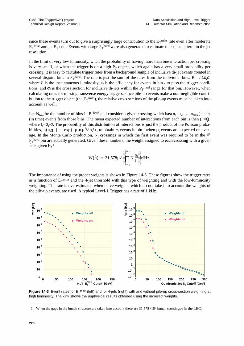
CMS: The Trigger/DAQ project Data Acquisition and High-Level TriggerTechnical Design Report, Volume II 14 Detector Simulation and Reconstruction
since these events turn out to give a surprisingly large contribution to the ETmiss rate even after moderate
ETmiss and jet ET cuts. Events with large PT
hard were also generated to estimate the constant term in the jetresolution.
In the limit of very low luminosity, when the probability of having more than one interaction per crossingis very small, or when the trigger is on a high PT object, which again has a very small probability percrossing, it is easy to calculate trigger rates from a background sample of inclusive di-jet events created inseveral disjoint bins in PT
hard. The rate is just the sum of the rates from the individual bins: R = LΣεiσiwhere L is the instantaneous luminosity, εi is the efficiency for events in bin i to pass the trigger condi-tions, and σi is the cross section for inclusive di-jets within the PT
hard range for that bin. However, whencalculating rates for missing transverse energy triggers, since pile-up events make a non-negligible contri-bution to the trigger object (the ET
miss), the relative cross sections of the pile-up events must be taken intoaccount as well.
Let Nbin be the number of bins in PThard and consider a given crossing which has
(in time) events from those bins. The mean expected number of interactions from each bin is then µi=fiµwhere fi=σi/σ. The probability of this distribution of interactions is just the product of the Poisson proba-bilities, , to obtain ni events in bin i when µi events are expected on aver-age. In the Monte Carlo production, Nj crossings in which the first event was required to be in the jth
PThard bin are actually generated. Given these numbers, the weight assigned to each crossing with a given is given by1
The importance of using the proper weights is shown in Figure 14-3. These figures show the trigger ratesas a function of ET
miss and the 4-jet threshold with this type of weighting and with the low-luminosityweighting. The rate is overestimated when naive weights, which do not take into account the weights ofthe pile-up events, are used. A typical Level-1 Trigger has a rate of 1 kHz.
1. When the gaps in the bunch structure are taken into account there are 31.578×10⁶ bunch crossings/s in the LHC.
Figure 14-3 Event rates for ETmiss (left) and for 4-jets (right) with and without pile-up cross-section weighting at
high luminosity. The kink shows the unphysical results obtained using the incorrect weights.
n1 n2 … nNbin ), , ,( n=
p ni µi;( ) µi–( ) µini ni!⁄( )exp=
n
W n( ) 31.578µ Njnj
fj
----
j 1=
Nbin
∏
⁄ MHz.=
1
10
10 2
10 3
10 4
10 5
10 6
10 7
10 8
10 9
0 50 100 150 200 250HLT ET
miss Cutoff [GeV]
Rat
e [H
z]
■ Weights off
● Weights on
10-2
10-1
1
10
10 2
10 3
10 4
10 5
10 6
10 7
10 8
10 9
0 50 100 150 200 250 300Quadruple Jet ET Cutoff [GeV]
Rat
e [H
z]
■ Weights off
● Weights on
228

CMS: The Trigger/DAQ project Data Acquisition and High-Level TriggerTechnical Design Report, Volume II 14 Detector Simulation and Reconstruction
14.1.4 Generation of Electron Trigger Samples
Jet background events for the electron/photon triggers are generated with PYTHIA in five bins of PThard.
A preselection is made at generator level to enrich the sample in events which will pass the Level-1 elec-tromagnetic trigger. It has been verified on a large unbiased sample that this preselection does not intro-duce significant bias.
A complication to the simulation of pile-up for the event sample used for electron and photon studies iscaused by minimum-bias events, generated as pile-up, that fire one arm of the Level-1 electron trigger.The events in the pile-up sample are reused many times. Generation of sufficient minimum-bias events toallow their use only once for the simulation of pile-up at high luminosity is not currently feasible, norwould it be an effective use of resources. But the reuse of pile-up events which themselves trigger leads tostatistical problems. The problem has been circumvented by excluding such events from the pile-up sam-ple. But this selection excludes a possible source of background. The magnitude of this excluded back-ground contribution has been estimated by calculating the probability, using a large unbiased sample offully simulated events, that a double electromagnetic trigger results from crossings in which one eventfires one arm and another event the other arm of the two electron trigger. For the high luminosity doubleelectron trigger threshold at 14 GeV, the excluded rate is found to be about 5% of the total.
14.2 Detector Description and Simulation (CMSIM)
The CMS simulation package, CMSIM [14-9], is an application of the GEANT3 [14-10] detector descrip-tion and simulation tool1. CMSIM is used to describe the detector geometry and materials. It also in-cludes, and uses, information about the magnetic field.
CMSIM reads the individual events from the CMKIN ntuple and simulates the effects of energy loss,multiple scattering and showering in the detector materials with GEANT3. The information is stored inthe form of “hits”. A simulated hit combines information about energy depositions in the detector, theirmagnitude, the time at which they occur and their location. The information stored in a hit is detector-de-pendent and contains all the details needed to simulate the detector response.
For tracking detectors (inner tracker and muon system) the information stored is the entry and exit pointsof the track, the momentum vector at the entry point, the type of the particle, the energy loss in the sensi-tive volume, and the time offset with respect to the trigger interaction time. For the calorimeters, the hitscontain summarized information about the energy (for HF the number of photoelectrons) deposited by ashower in a crystal or a scintillator and the time slice during which that happened. A time slice is an inter-val of 1 ns. Finally, a number to identify the detector element that contains the hit is stored. Two calorim-eter hits are distinct when they originate from different particles — even if this happens at the same timeand in the same detector element.
In addition to the hits, CMSIM also produces simulated tracks and vertices. These are not used for detec-tor response simulation or for reconstruction, but are required for analysis of the reconstruction results.They constitute the “Monte Carlo truth” about the interactions and decays of particles in the detector.
The results of the simulation are stored in GEANT3/CMSIM data structures in the form of ZEBRAbanks. Interface routines similar to GS- and GF-routines in GEANT3 are provided for users to access datastructures without knowledge of the ZEBRA memory management system. The information stored in theZEBRA files is then imported into ORCA and stored in the Objectivity/DB databases. The average stor-
1. CMSIM also includes code for reconstruction and analysis which is, however, not used any more.
229

CMS: The Trigger/DAQ project Data Acquisition and High-Level TriggerTechnical Design Report, Volume II 14 Detector Simulation and Reconstruction
age size of a single event is 2 MB. The CPU time required to simulate one event on a 1 GHz Pentium-IIICPU ranges from 60 s for a minimum-bias event, to 500 s for a 1 TeV jet-jet event.
All results presented in this TDR are, unless otherwise specified explicitly, simulated with versionCMSIM125 of the CMSIM package.
In what follows, the CMS coordinate system is defined as follows: the z-axis is parallel to the beam axisand the magnetic field of the solenoid, and the polar angle theta is defined with respect to it. The azimuth-al angle around the z-axis is denoted by the symbol φ, and the pseudorapidity -log(tan(θ/2) is denoted bythe symbol η. The symbol PT is used to denote the component of momentum transverse to the z-axis.
14.2.1 Tracker Geometry and Simulation
In the original design, the CMS Tracking detector consisted of a pixel vertex detector, a silicon Microstripdetector and MSGC gas detectors in the outer layers. In 2000 an addendum to the original design of theCMS tracker was approved. In the new design, the outer MSGC layers were substituted by other layers ofsilicon microstrips leading to an all-silicon configuration. The layout of the all-silicon tracker was subse-quently optimized, before finally being frozen in the fall of 2001. It is this final layout that is used in thesimulations described in this chapter.
In this configuration, the tracker detector has three pixel layers and ten silicon strip layers in the barrel,plus two pixel layers, three inner and nine outer forward disks of silicon detectors in each end-cap, asshown in Figure 14-4. The outer radius of the CMS tracker extends up to 107–110 cm. The length of thetracker is approximately 540 cm.
The tracker contains a total of 15148 silicon strip modules with sensors whose thickness and pitch are list-ed in Table 14-1.
The pixel detector provides high resolution 3D space points required for the charged track pattern recog-nition. Due to its high position resolution (≈15 µm in both coordinates) it can determine the impact pa-rameter of charged particles with high precision. It will also allow vertex reconstruction in threedimensions and will permit identification of b and tau-jets.
Figure 14-4 r-z view of a quadrant of the silicon part of the tracker. The inner barrel (TIB) has four layers, theouter barrel (TOB) has six layers. The inner (TID) end cap is made of three small disks on each side of the innerbarrel. The outer end-cap (TEC) is made of nine big disks on both sides of the tracker.
230

CMS: The Trigger/DAQ project Data Acquisition and High-Level TriggerTechnical Design Report, Volume II 14 Detector Simulation and Reconstruction
The pixel detector consists of three barrel layers with two end-cap disks on each side (Figure 14-5 left).The three barrel layers will be located at mean radii of 4.4 cm, 7.3 cm and 10.2 cm respectively, and willbe 53 cm long. The two end disks, extending from 6 to 15 cm in radius, will be placed on each side atz=34.5 cm and 46.5 cm. For the initial low luminosity runs the pixel detector will be staged to two barrellayers and one end-cap disk only.
In order to achieve the optimal vertex position resolution in both the (r, φ) and the z coordinates a designwith a square pixel shape 150×150 µm2 was adopted. To enhance the spatial resolution by analogue sig-nal interpolation the effect of charge sharing induced by the large Lorentz drift in the 4 T magnetic field isused. Hence the detectors are deliberately not tilted in the barrel layers but are tilted in the end disks re-sulting in a turbine-like geometry. The whole pixel system consists of about 1400 detector modules ar-ranged into half-ladders of 4 identical modules each in the barrel and blades with 7 different moduleseach in the disks. To read out the detector about 16000 readout chips are bump-bonded to the detectormodules. The total number of readout channels (pixels) is about 44×106.
The pixel detector has been designed to provide 2 hit coverage up to rapidities of about η=2.2 (for tracksoriginating within 2σ around the centre). This is illustrated in Figure 14-5 (right, upper plot) where the ef-ficiency for 2 hits is shown for the 3 barrel + 2 disk configuration. The efficiency is calculated for hightransverse momentum muons originating from primary vertices smeared along the z axis with σ=5.3 cm,
Table 14-1 Detectors types in the silicon tracker.
part detectors thickness (µm) pitch (µm)
Inner barrel 2724 320 81/118
Outer barrel 5208 500 123/183
Inner disks 816 300 97/128/143
Outer disks 2512 300 96/126/128/143
Outer disks (2) 3888 500 143/158/183
Figure 14-5 Left: illustration of the pixel detectors in the CMS tracker. Right: the efficiency for obtaining 2 (upperplot) and 3 (lower plot) pixel hits as a function of rapidity. The solid line is the three barrels + two disks configura-tion, the dashed line is for two barrels + one disk and the dotted line for three barrels + three disks.
2 and 3 hit pixel efficiency
231

CMS: The Trigger/DAQ project Data Acquisition and High-Level TriggerTechnical Design Report, Volume II 14 Detector Simulation and Reconstruction
but with a cutoff at 2σ. The staged, 1 disk configuration, limits the coverage to |η|=2.0. Note that the fullcoverage up to |η|=2.4 can be achieved with an upgrade to 3 disks. For stand-alone pixel tracking capabil-ities one needs at least 3 pixel hits per track. This can be achieved with the 3 barrel layers available for thehigh luminosity runs. The 3-hit coverage is also shown in Figure 14-5 (right, lower plot).
14.2.1.1 Tracker Material
The CMS tracker clearly includes both sensitive detector volumes and non-sensitive ones. Due to the factthat the tracker requires ~15 kA of low voltage current supply and dissipates approximately 60kW ofpower, a large fraction of the material consists of electrical supply cables and cooling services. Othernon-sensitive material parts are cables, support structures, electronics, the beam-pipe and the thermalscreen outside the tracker. The GEANT3/CMSIM simulation of the CMS tracker is tuned to describe allof these components to a high level of accuracy. Figure 14-6 (left) shows a simulated TOB detector rod,with the mother cable, cooling and electronics.
Figure 14-6 (right) shows examples of the simulated tracker volume (TIB and TOB). The readout elec-tronics, the cooling and support structure reflect the current technical designs.
The decomposition of the tracker material in units of radiation lengths and in units of absorption lengthsversus η for the different subdetectors is shown in Figure 14-7
14.2.2 ECAL Geometry and Simulation
The nominal (engineering specification) geometry of the ECAL is simulated in fine detail in theGEANT3/CMSIM model. Figure 14-8 shows a transverse section of the ECAL, including the end-cappreshower detector, as it is described in GEANT3/CMSIM.
The sizes and positions of ECAL barrel (|η| < 1.479) crystals are unchanged since the ECAL TDR[14-11]. Each half barrel consists of 18 super-modules each containing 20×85 crystals. The crystals are
Figure 14-6 Examples of tracker volumes simulated in CMSIM. Left: a simulated TOB Rod; right: the Inner Bar-rel (TIB) and Outer Barrel (TOB) modules.
TIB module
TOB module
232

CMS: The Trigger/DAQ project Data Acquisition and High-Level TriggerTechnical Design Report, Volume II 14 Detector Simulation and Reconstruction
tilted so that their axes make an angle of 3° with a line from the nominal vertex point, and each covers ap-proximately 0.0174×0.0174 in η−φ. This is achieved using 17 pairs (left and right stereo images) of dif-ferent crystal shapes. The crystals are 230 mm (25.8 X0) in length. They are contained in a thin walledglass-fibre alveola structure. There is a light and thin structure in front of the crystals acting as a thermalshield and neutron moderator, which also carries the light fibres used for the laser-based monitoring sys-tem. All this is described and simulated in fine detail in the geometry model, together with the electronics,
Figure 14-7 Material budget as a function of η for the different tracker subunits. On the left: material thicknessin units of radiation length versus η. On the right: material thickness in units of interaction length versus η.
Figure 14-8 Transverse section of ECAL, as described in GEANT3/CMSIM (version CMS125).
y
z
Preshower (SE)
Barrel ECAL (EB)
Endcap
η = 1.653
η = 1.479
η = 2.6η = 3.0
ECAL (EE)
233

CMS: The Trigger/DAQ project Data Acquisition and High-Level TriggerTechnical Design Report, Volume II 14 Detector Simulation and Reconstruction
the thermal regulation system and mechanical structures behind, as well as the mechanical structure sepa-rating the four modules which make up each super-module.
The end-cap consists of identically shaped crystals, slightly shorter (220 mm, 24.7 X0) and somewhatlarger in cross-section than the barrel crystals, grouped in mechanical units of 5×5 crystals (super-crys-tals) consisting of a carbon-fibre alveola structure. The crystals and super-crystals are arranged in a rec-tangular x-y grid, with the crystal axes off-pointing from the nominal vertex by angles between 2° and 5°.The end-cap mechanical design details, crystal sizes and the precise positioning of the super-crystals havebeen slightly revised since the ECAL TDR. In front of most of the end-cap (|η| > 1.653) there is a 3X0preshower detector, consisting of lead radiators and two orthogonal planes of silicon strip detectors. As inthe case of the barrel, the model of the geometry contains all these details together with a description ofthe mechanical structures and thermal regulation structures, and a less detailed modelling of the electron-ics behind them.
The active volumes of the ECAL, for which the deposited energy is recorded (i.e. the output of theGEANT3/CMSIM step in the simulation chain), are the crystals and the silicon strips. The arrival time ofhits, as well as the energy deposited, is recorded. For the crystals the variation of the light collection effi-ciency along the length of the crystal is simulated by multiplying the energy, as it is deposited, by a nom-inal longitudinal light collection curve. This is a simple function of the distance from the crystalfront-face, and is flat in the front half of the crystal, with a 5% linear rise over the rearmost 100 mm. De-viations from this nominal curve, as measured on production crystals, which deteriorate the energy reso-lution, are accounted for by a random smearing which is added later to the energy (see Section 14.3.1.4).Further discussion of longitudinal non-uniformity of light collection can be found in [14-12] and refer-ences listed therein.
14.2.3 HCAL Geometry and Simulation
The CMS hadronic calorimeter consists of four detectors, the barrel (HB), outer barrel (HO), end-cap(HE), and forward calorimeter (HF). The HB and the HE are inside the superconducting solenoid whereasthe HO resides inside the return yoke of the magnet. The forward calorimeter is located beyond the returnyoke of the magnet at a distance of 11.15 m from the center of CMS.
The HB covers the pseudorapidity region |η| < 1.740. The central barrel is divided into two half-sectionseach consisting of 18 identical wedges in φ. Each wedge consists of 17 sampling layers and these layersare ganged together as a single tower in the readout. There are cutouts at η = 1.2 for the routing of innerdetector cables and after layer 16 for a patch panel. The absorber and scintillator plates are staggered in φ.The scintillator “megatiles” are made of scintillator wrapped in plastic. The first and last sampling layerhave 8mm thick scintillator, the rest 4 mm. The first absorber layer is iron, and all subsequent ones brassof thickness 60 mm (first 9 layers) and 66 mm (the remaining 6 layers).
The HE covers the region 1.305 < |η| < 3.0, overlapping with the HB in the region 1.305 < |η| < 1.740. Itis divided into a backward and a forward unit, each containing 18 wedges. The wedges have 19 layers ofabsorber and scintillator. The front layer of scintillator is 9 mm thick, subsequent ones are 4 mm thick.The absorber is in the form of 80 mm thick brass plates.
The HF covers the region 2.853 < |η| < 5.191. It is located between 11.15 m and 12.80 m from the inter-action region, and is made out of 18 iron wedges. The detector measures signals produced by Cerenkovradiation in quartz fibers. The forward calorimeter is longitudinally separated into two compartments, anelectromagnetic section corresponding to 16 radiation lengths, and a hadronic section corresponding toapproximately 9 interaction lengths.
234
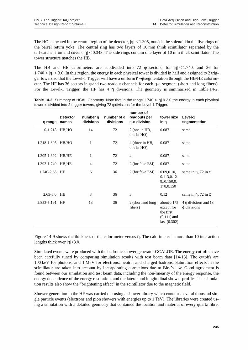
CMS: The Trigger/DAQ project Data Acquisition and High-Level TriggerTechnical Design Report, Volume II 14 Detector Simulation and Reconstruction
The HO is located in the central region of the detector, |η| < 1.305, outside the solenoid in the five rings ofthe barrel return yoke. The central ring has two layers of 10 mm think scintillator separated by thetail-catcher iron and covers |η| < 0.348. The side rings contain one layer of 10 mm thick scintillator. Thetower structure matches the HB.
The HB and HE calorimeters are subdivided into 72 φ sectors, for |η| < 1.740, and 36 for1.740 < |η| < 3.0. In this region, the energy in each physical tower is divided in half and assigned to 2 trig-ger towers so that the Level-1 Trigger will have a uniform η−φ segmentation through the HB/HE calorim-eter. The HF has 36 sectors in φ and two readout channels for each η-φ segment (short and long fibers).For the Level-1 Trigger, the HF has 4 η divisions. The geometry is summarized in Table 14-2.
Figure 14-9 shows the thickness of the calorimeter versus η. The calorimeter is more than 10 interactionlengths thick over |η|<3.0.
Simulated events were produced with the hadronic shower generator GCALOR. The energy cut-offs havebeen carefully tuned by comparing simulation results with test beam data [14-13]. The cutoffs are100 keV for photons, and 1 MeV for electrons, neutral and charged hadrons. Saturation effects in thescintillator are taken into account by incorporating corrections due to Birk’s law. Good agreement isfound between our simulation and test beam data, including the non-linearity of the energy response, theenergy dependence of the energy resolution, and the lateral and longitudinal shower profiles. The simula-tion results also show the “brightening effect” in the scintillator due to the magnetic field.
Shower generation in the HF was carried out using a shower library which contains several thousand sin-gle particle events (electrons and pion showers with energies up to 1 TeV). The libraries were created us-ing a simulation with a detailed geometry that contained the location and material of every quartz fibre.
Table 14-2 Summary of HCAL Geometry. Note that in the range 1.740 < |η| < 3.0 the energy in each physicaltower is divided into 2 trigger towers, giving 72 φ divisions for the Level-1 Trigger.
η rangeDetector names
number η divisions
number of ϕ divisions
number of readouts perη-ϕ division
tower size in η
Level-1 segmentation
0-1.218 HB,HO 14 72 2 (one in HB, one in HO)
0.087 same
1.218-1.305 HB/HO 1 72 4 (three in HB, one in HO)
0.087 same
1.305-1.392 HB/HE 1 72 4 0.087 same
1.392-1.740 HB,HE 4 72 2 (for fake EM) 0.087 same
1.740-2.65 HE 6 36 2 (for fake EM) 0.09,0.10, 0.113,0.129,.0.150,0.178,0.150
same in η, 72 in φ
2.65-3.0 HE 3 36 3 0.12 same in η, 72 in φ
2.853-5.191 HF 13 36 2 (short and long fibers)
about 0.175 except for the first (0.111) and last (0.302)
4 η divisions and 18 ϕ divisions
235

CMS: The Trigger/DAQ project Data Acquisition and High-Level TriggerTechnical Design Report, Volume II 14 Detector Simulation and Reconstruction
Cerenkov photon emission and transmission in the fibres were modelled in detail. The results obtainedfrom the shower library closely match those from the detailed simulation [14-14].
14.2.4 Muon Chamber Geometry and Simulation
There are three muon systems in CMS: a barrel muon system composed of drift tubes (DT) in the centralregion (|η|<1.2), an end-cap muon system composed of cathode strip chambers (CSC) in the forward re-gion (0.9<|η|<2.4), and resistive plate chambers (RPC) deployed throughout the central and forward re-gions (|η|<2.1). A longitudinal view of the three muon systems is shown in Figure 14-10.
Figure 14-9 Material budget plot as a function of η through the last layer of the hadron calorimeter.
Figure 14-10 Cross-sectional view of one quarter of CMS showing the DT, CSC, and RPC muon systems.
0
2
4
6
8
10
12
14
16
18
20
0 1 2 3
Inner insensitiveInner sensitiveOuter insensitiveOuter sensitive
cmsim 125
η
λ/λ 0
0
100
200
300
400
500
600
700
800
0 200 400 600 800 1000 1200Z (cm)
R (
cm)
RPC
CSC
Drift Tubes η = 1.04
η = 2.4�
MB 2/1�
MB 2/2
ME
1/1�
ME
1/2�
ME
1/3
�
ME
2/2
��
� ME
3/2
�
ME
4/2
�
ME
2/1
��
� ME
4/1
�
ME
3/1
MB 2/3
MB 2/4
MB 1/1�
MB 1/2�
MB 1/3�
MB 1/4�
236

CMS: The Trigger/DAQ project Data Acquisition and High-Level TriggerTechnical Design Report, Volume II 14 Detector Simulation and Reconstruction
The drift-tube system of CMS is segmented into 5 iron wheels along the beam axis, each 2.5 m in width,with chambers arranged in 4 stations at different radii (MB1−MB4) within each wheel. Each station issubdivided in azimuth into 12 sectors, with a single chamber mounted into each sector except for the topand bottom sectors of MB4, which have been split into two chambers. The total number of DT chambersis thus 250. A single DT chamber is composed of three superlayers of drift-tubes (two to measure the φcoordinate and one to measure z), where a superlayer is composed of four layers of drift-tubes. The outer-most station, MB4, has only the 2 superlayers for the measurement of the φ coordinate. The transverse di-mensions of a single drift cell, shown in Figure 14-11, measure 42 mm by 13 mm, and the wire lengthvaries from 2 to 4 m.
The cathode strip chamber system of CMS contains four stations (ME1−ME4) of chambers mounted onthree iron disks perpendicular to the beamline on each end of the apparatus (see Figure 14-10). The fourthCSC station, ME4, is staged in the current planning and will not be available for initial low luminosityrunning, but is included in the HLT simulations for which the results are described here. A single CSCstation is composed of two rings of chambers (three for ME1), where each chamber has six active gas lay-ers. A single layer has a gap thickness of 9.5 mm, cathode strips aligned radially with a pitch that variesfrom 7 to 16 mm, and anode wires aligned in the orthogonal direction with a pitch of 3.2 mm (but gangedinto groups of 5−16 wires for readout). Each chamber is trapezoidal in shape with either a 10° or 20° an-gular coverage in azimuth (φ), depending on the ring and station, with the largest chambers measuring3.4 m in length and 1.5 m in width. The complete system contains a total of 540 chambers. The chambersin the innermost ring of the first station (ME 1/1) are segmented into two regions in radius. The most for-ward of these two regions (|η|>2.1) is not expected to participate in the Level-1 Trigger.
The resistive plate chamber system in the barrel has six radial stations placed within the same 5 wheels asthe DT system (two RPC chambers in both the MB1 and MB2 stations, and one chamber each for MB3and MB4). In the end-caps, the RPC system shares the same four stations as the CSC system. The cham-bers are a double-gap design, with a common pick-up segmented into strips that are rectangular in the bar-rel and trapezoidal in the end-caps. The gap thickness is 2 mm. The total number of chambers is 612.
The simulated hit (a “SimHit”) of a charged particle crossing an active layer in each of the three muonsystems contains the entry and exit points for each active gas layer. GEANT3 is not used to model the in-teraction of this primary particle in the gas, only to estimate its energy loss. The interaction in the gas it-
Figure 14-11 Transverse view of a drift-tube cell, with drift lines and isochrones for a typical voltage configura-tion of the electrodes.
237
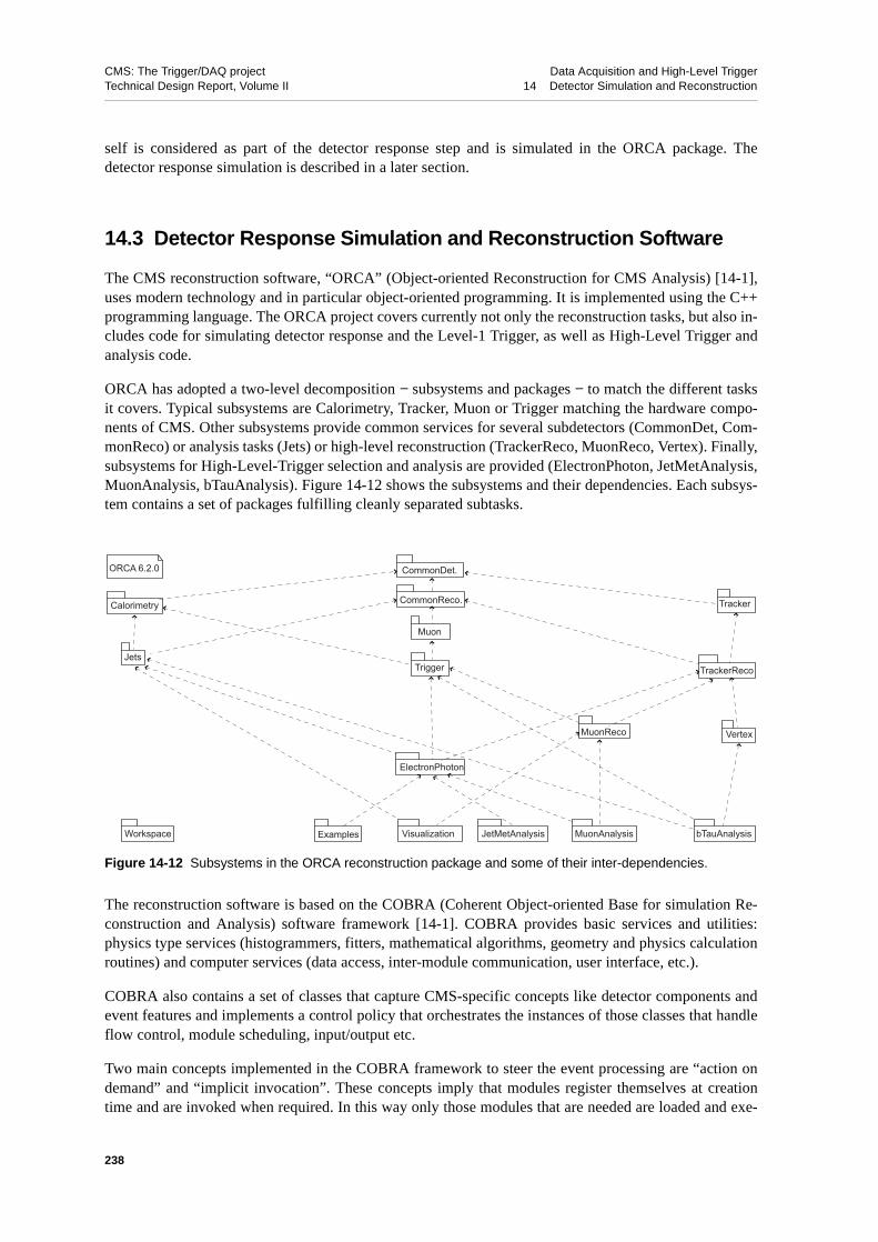
CMS: The Trigger/DAQ project Data Acquisition and High-Level TriggerTechnical Design Report, Volume II 14 Detector Simulation and Reconstruction
self is considered as part of the detector response step and is simulated in the ORCA package. Thedetector response simulation is described in a later section.
14.3 Detector Response Simulation and Reconstruction Software
The CMS reconstruction software, “ORCA” (Object-oriented Reconstruction for CMS Analysis) [14-1],uses modern technology and in particular object-oriented programming. It is implemented using the C++programming language. The ORCA project covers currently not only the reconstruction tasks, but also in-cludes code for simulating detector response and the Level-1 Trigger, as well as High-Level Trigger andanalysis code.
ORCA has adopted a two-level decomposition − subsystems and packages − to match the different tasksit covers. Typical subsystems are Calorimetry, Tracker, Muon or Trigger matching the hardware compo-nents of CMS. Other subsystems provide common services for several subdetectors (CommonDet, Com-monReco) or analysis tasks (Jets) or high-level reconstruction (TrackerReco, MuonReco, Vertex). Finally,subsystems for High-Level-Trigger selection and analysis are provided (ElectronPhoton, JetMetAnalysis,MuonAnalysis, bTauAnalysis). Figure 14-12 shows the subsystems and their dependencies. Each subsys-tem contains a set of packages fulfilling cleanly separated subtasks.
The reconstruction software is based on the COBRA (Coherent Object-oriented Base for simulation Re-construction and Analysis) software framework [14-1]. COBRA provides basic services and utilities:physics type services (histogrammers, fitters, mathematical algorithms, geometry and physics calculationroutines) and computer services (data access, inter-module communication, user interface, etc.).
COBRA also contains a set of classes that capture CMS-specific concepts like detector components andevent features and implements a control policy that orchestrates the instances of those classes that handleflow control, module scheduling, input/output etc.
Two main concepts implemented in the COBRA framework to steer the event processing are “action ondemand” and “implicit invocation”. These concepts imply that modules register themselves at creationtime and are invoked when required. In this way only those modules that are needed are loaded and exe-
Figure 14-12 Subsystems in the ORCA reconstruction package and some of their inter-dependencies.
ORCA 6.2.0
Calorimetry
Jets
Workspace Examples
CommonDet.
CommonReco.
Muon
Trigger
MuonReco
Tracker
TrackerReco
Vertex
Visualization JetMetAnalysis MuonAnalysis bTauAnalysis
ElectronPhoton
238

CMS: The Trigger/DAQ project Data Acquisition and High-Level TriggerTechnical Design Report, Volume II 14 Detector Simulation and Reconstruction
cuted. Implicit invocation uses additional mechanisms to construct the required modules, to customizethem and to manage dependencies among them. Modules whose change of state depends on the occur-rence of some external “event” register as “observers” to the “dispatcher” of such an “event”. Typical“events” are the reading of a new physics event from the detector, a new run or a new detector setup. Onthe arrival of a new “event” the dispatcher informs all registered observers. These can then update theirstate accordingly and eventually perform a specific action (like the reconstruction of some object, see be-low). To avoid useless computation, such an action can be deferred until a client asks an observer for aservice (e.g. the delivery of some reconstructed tracks).
14.3.1 Simulation of Detector Response (DIGI Creation)
After combining a signal event with the selected pile-up events for a particular luminosity, the detector re-sponse is simulated taking into account the simulated hits of all events of a crossing. The time informa-tion of each hit is shifted according to the bunch crossing to which the corresponding event belongs.
The finite response time and time resolution of the CMS subdetectors defines for each subdetector a timewindow of sensitivity, ranging from a few tens of nanoseconds to several hundred nanoseconds. To simu-late the full detector response and occupancy, simulated hits in the full time interval of sensitivity need tobe taken into account.
The simulation of the detector response is different for each subdetector and is described in the followingsections.
14.3.1.1 Pile-up Treatment
The LHC luminosity is such that a number of pp collisions occur each bunch crossing. In most of thesecollisions “minimum-bias” events are produced. For the simulation these “minimum-bias” or “pile-up”events are distinguished from hard scattering events that trigger the detector readout. The latter are re-ferred to as “trigger” or “signal” events.
Because there is only 25 ns between consecutive bunch crossings, the CMS detector will integrate overpile-up events produced before and after the signal event. In total up to about 160 pile-up events need tobe overlaid with a single signal event to properly simulate the detector response at high luminosity.
The number of bunch crossings to be piled-up is determined by the subdetector with the slowest responsetime. The values used are -5 to +3, i.e. five bunch crossings preceding the trigger bunch crossing, and 3following it. This also takes into account most signals generated by soft particles looping in the detector.
For each crossing an individual signal event is combined with a random set of minimum-bias events takenfrom a pool of pile-up events. The size of the pool of pile-up events is chosen to be large enough to ensurea unique combination for each crossing. This “recycling” of pile-up events is needed due to the limitedCPU resources available.
14.3.1.2 Pixel Detector Response
The entrance and exit points in the pixel sensitive volumes, together with the deposited energy, are re-corded during the GEANT track propagation, providing input information for signal simulation. Thetrack segment inside the sensor volume is divided into 10 µm long subsegments. Each subsegment is as-signed a fraction of the energy using the GEANT3 routine GLANDZ [14-15]. This distribution takes intoaccount Landau fluctuations in thin material layers.
239

CMS: The Trigger/DAQ project Data Acquisition and High-Level TriggerTechnical Design Report, Volume II 14 Detector Simulation and Reconstruction
The charge from each track subsegment is drifted to the detector surface and simultaneously diffused inthe perpendicular plane. The diffusion is assumed to be Gaussian and is proportional to the square-root ofthe drift length. The diffusion constant is normalized to 7 µm for a 300 µm thick detector. The finalcharge distribution on the detector surface is calculated as a sum of two-dimensional Gaussian distribu-tions. The magnitude of the Lorentz drift in 4 T magnetic field is defined by the drift length and theLorentz angle, which depends on the strength of the magnetic field.
The resulting two dimensional charge distribution is mapped to the pixel geometry and the fraction ofcharge collected by each pixel is determined. The cut-off value for integration of the charge distribution is5 σ. A list of hit pixels for all contributing tracks is formed. If a single pixel is hit by more than one track,the charge contributions are added together.
The noise is assumed to be Gaussian, centred at zero. All hit pixels have the noise contribution added tothem. In addition, noisy pixels with charge amplitude larger than the pixel threshold are generated accord-ing to the tail of the Gaussian distribution. The default noise used in the simulation is σ=500 electrons.
To digitize the signal collected in each pixel, the charge is multiplied by a gain factor and converted intoan integer number, so simulating ADC digitization. Signals which exceed the ADC range are assigned asaturation value which depends on the ADC maximum bit number. Both the gain and the number of ADCbits (typically 6) can be adjusted. Pixel zero-suppression is simulated by comparing the digitized signal toa threshold for each channel (Figure 14-13). The peak close to 35000 electrons corresponds to signal sat-uration and that at 1000 electrons is due to noise. The threshold is defined in units of noise and is typicallyset at 5 σ (2500 electrons).
The finite space available in the pixel readout chip requires the size of data buffers, and the complexity ofthe circuits, to be carefully optimized. Although the readout efficiency has been maximized, some datalosses will always be present. Additional pixel inefficiencies are expected due to unbonded and noisy pix-els. To simulate such inefficiencies, randomly chosen pixels are erased. In addition some pixel dou-ble-columns and some whole readout chips are cleared as well. The data losses are in general dependenton the CMS trigger rate, LHC luminosity and the module distance from the interaction point. They wereparameterized according to results obtained from detailed simulations and included in the ORCA digitiza-tion code.
Figure 14-13 shows the simulated charge distribution for minimum-bias events and for single muontracks (100 GeV). Part a) of the figure shows the total charge deposited in the pixel barrel by mini-mum-bias (solid line) and muon (dashed) tracks. The edge at 18000 electrons corresponds to a mip signal.Part b) shows the signal seen by a single barrel pixel for 125 µm and for 150 µm pixels. The average sig-nal is about 12000 electrons, which corresponds to the S/N ratio assumed in this simulations of 24:1.
Figure 14-14 shows the average number of hit pixels in the pixel barrel layer at 7 cm as a function of ra-pidity for single muon tracks (100 GeV). The pixel cluster size in r-φ is determined by the Lorentz shiftand is about 2 pixels for the whole rapidity range. The cluster size in the z coordinate is determined most-ly by the track impact angle and varies with rapidity from 1 to 6. In this case all tracks are assumed tooriginate from the detector centre (no vertex smearing).
14.3.1.3 Silicon Microstrips Detector Response
The entry and exit points, as well as the energy deposited in the silicon (Eion) by the incident particle, areprovided by the GEANT3 package during track propagation in CMSIM.
The signal from real silicon detectors is processed by the APV25 readout chip [14-16] [14-17]. Thefinite shaping time of this amplifier is the primary cause of signal pile-up from out-of-time bunch cross-
240

CMS: The Trigger/DAQ project Data Acquisition and High-Level TriggerTechnical Design Report, Volume II 14 Detector Simulation and Reconstruction
ings. The APV25 will usually operate in “deconvolution mode”, since this gives it the best time resolu-tion. Figure 14-15 shows the APV time response, fitted with a Gaussian of width 12.1 ns [14-16][14-17].The software simulates the dependence on the pile-up arrival time, by weighting the energy loss from
Figure 14-13 a) Simulated charge distribution deposited by minimum-bias tracks (solid line) in a 250 µm barreldetector at a radius of 7 cm. For comparison, charge from 100 GeV muon tracks at normal incidence is alsoshown (dashed line). b) Simulated charge distribution seen by a single barrel pixel 125 µm (solid line) and150 µm (dashed line) large.
Figure 14-14 Average number of pixels hit in the barrel layer at 7 cm (pixel size 150 µm) versus rapidity for asingle 100 GeV muon track. The solid line (triangles) is for a fully depleted detector (250 µm) and the dashedline (squares) is for a detector with partial depletion of 200 µm.
Track charge /electrons
Arb
itra
ry u
nit
s
Pixel charge /electrons
Arb
itra
ry u
nit
s
0
200
400
600
800
1000
1200
x102
0 40000 80000
105
106
0 20000 40000
r pixel multiplicity
0
0.5
1
1.5
2
2.5
3
0 0.5 1 1.5 2
Rapidity
z pixel multiplicity
0
1
2
3
4
5
6
7
0 0.5 1 1.5 2
Rapidity
250
250
200
200
φ
241
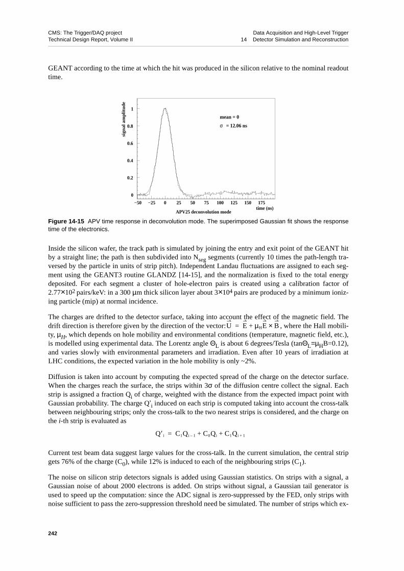
CMS: The Trigger/DAQ project Data Acquisition and High-Level TriggerTechnical Design Report, Volume II 14 Detector Simulation and Reconstruction
GEANT according to the time at which the hit was produced in the silicon relative to the nominal readouttime.
Inside the silicon wafer, the track path is simulated by joining the entry and exit point of the GEANT hitby a straight line; the path is then subdivided into Nseg segments (currently 10 times the path-length tra-versed by the particle in units of strip pitch). Independent Landau fluctuations are assigned to each seg-ment using the GEANT3 routine GLANDZ [14-15], and the normalization is fixed to the total energydeposited. For each segment a cluster of hole-electron pairs is created using a calibration factor of2.77×102 pairs/keV: in a 300 µm thick silicon layer about 3×10⁴ pairs are produced by a minimum ioniz-ing particle (mip) at normal incidence.
The charges are drifted to the detector surface, taking into account the effect of the magnetic field. Thedrift direction is therefore given by the direction of the vector: , where the Hall mobili-ty, µH, which depends on hole mobility and environmental conditions (temperature, magnetic field, etc.),is modelled using experimental data. The Lorentz angle ΘL is about 6 degrees/Tesla (tanΘL=µHB=0.12),and varies slowly with environmental parameters and irradiation. Even after 10 years of irradiation atLHC conditions, the expected variation in the hole mobility is only ~2%.
Diffusion is taken into account by computing the expected spread of the charge on the detector surface.When the charges reach the surface, the strips within 3σ of the diffusion centre collect the signal. Eachstrip is assigned a fraction Qi of charge, weighted with the distance from the expected impact point withGaussian probability. The charge Q’i induced on each strip is computed taking into account the cross-talkbetween neighbouring strips; only the cross-talk to the two nearest strips is considered, and the charge onthe i-th strip is evaluated as
Current test beam data suggest large values for the cross-talk. In the current simulation, the central stripgets 76% of the charge (C0), while 12% is induced to each of the neighbouring strips (C1).
The noise on silicon strip detectors signals is added using Gaussian statistics. On strips with a signal, aGaussian noise of about 2000 electrons is added. On strips without signal, a Gaussian tail generator isused to speed up the computation: since the ADC signal is zero-suppressed by the FED, only strips withnoise sufficient to pass the zero-suppression threshold need be simulated. The number of strips which ex-
Figure 14-15 APV time response in deconvolution mode. The superimposed Gaussian fit shows the responsetime of the electronics.
APV25 deconvolution mode
0
0.2
0.4
0.6
0.8
1
−50 −25 0 25 50 75 100 125 150 175time (ns)
sig
na
l am
plit
ud
eσ
mean = 0
= 12.06 ns
U E µHE B×+=
Q ′ i C1Qi 1– C0Qi C1Qi 1++ +=
242

CMS: The Trigger/DAQ project Data Acquisition and High-Level TriggerTechnical Design Report, Volume II 14 Detector Simulation and Reconstruction
ceed the threshold is calculated using Poisson statistics, and a noise exceeding the threshold is simulatedonly for this small subset of strips (about 5% with the standard threshold cut at 2σ).
An alternative and more realistic operating mode can optionally be enabled in the simulation, which ac-counts for effects due to the overall electronics chain. In this mode, the noise is simulated on each strip,together with common mode noise and pedestals as obtained from laboratory measurements. The FEDcommon mode and zero-suppression algorithms are simulated at the APV (128 strips) level, as are possi-ble algorithms which could be used to calibrate the pedestals and noise. This allows the study of algo-rithms to be implemented in the FED and in the FED crate controller. The simulation shows that thecurrently proposed common mode subtraction algorithm will function correctly at CMS, and initial re-sults on possible pedestal and noise calibration algorithms are encouraging (Figure 14-16).
The FED implements a zero-suppression algorithm to limit the data rate from the tracker: a strip is accept-ed only if the significance of its signal exceeds 5σ, or if it exceeds 2σ and is part of a cluster. This algo-rithm has been implemented in the software simulation.
By taking into account all estimates reported in this section, a signal to noise ratio of 12 to 14 is obtainedfor tracks at normal incidence. The signal to noise ratio is defined here as the ratio of the most probablecluster charge to the noise of one strip. Figure 14-17 shows the S/N shape, with tails due to Landau fluc-tuations.
14.3.1.4 ECAL Detector Response
The ECAL detector response simulated in ORCA consists of:
• simulation of the digitization of hits by the readout electronics;
Figure 14-16 Reconstructed noise and pedestals in a TOB detector, estimated using a calibration algorithm ona sample of 300 minimum-bias events. The true values of the noise and pedestal, input to the simulation, are100 and 24 respectively.
0 2 4 6 8
10 12 14
x 10 4
90 92.5 95 97.5 100 102.5 105 107.5 110
ADC counts
0 1 2 3 4 5 6 7 8
16 18 20 22 24 26 28 30 32
ADC counts
x 10 4
Arb
itrar
y U
nits
Arb
itrar
y U
nits
243

CMS: The Trigger/DAQ project Data Acquisition and High-Level TriggerTechnical Design Report, Volume II 14 Detector Simulation and Reconstruction
• addition of Gaussian random smearing to the energy, to account for electronics noise, intercalibra-tion uncertainty, crystal deviations from the nominal longitudinal light collection curve, and photo-statistics.
Since the ECAL front-end electronics is specified such that digitization noise will make a negligible con-tribution to the errors on the measured energy, the main function of the digitization simulation for theHLT work is to provide a realistic modelling of out-of-time pile-up, i.e. pile-up from bunch crossings oth-er than the one in which the Level-1 Trigger occurs. A function is used to describe the time developmentof the signals from the ECAL FPPA. When used together with the recorded time at which the energy wasdeposited, and sampled at 40 MHz, the observable time frames can be simulated. These time frames, con-sisting of 10 time samplings1, correspond to the raw data which will be input to the HLT farm. The simu-lation of the preshower detector follows the same pattern, although the time development of the signals isfaster, and the time frames consist of only 3 time samples.
In current practice, for reasons of technical simplicity and simulation speed, the Gaussian random smear-ings are added to the energy reconstructed from the time frames (see Section 14.3.2.2) rather than to thedeposited energy before the simulation of the time frames. Table 14-3 lists the Gaussian smearings added.It is interesting to note that, since the ECAL is a homogeneous electromagnetic calorimeter, these smear-ing dominate the energy resolution for unconverted photons in the barrel. For example, making the sim-plified approximation that most of the energy is deposited in a single crystal, the smearing detailed belowgives a resolution of about 0.8% for a 35 GeV photon reconstructed in 5×5 crystals, as compared to about0.9% measured with full simulation.
Figure 14-17 S/N ratio for silicon microstrip detectors. All energy losses are scaled to perpendicular impact.
1. Although it is intended to record a full 10 time samples, the reconstruction used for the HLT studies used only 8.
Table 14-3 Gaussian smearing applied to the energy deposited in ECAL (for the preshower the value given isexpressed in terms of reconstructed energy).
Barrel End-cap preshower
Electronics noise σ = 40 MeV σ = 150 MeV σ = 4 MeV
Photostatistics (E in GeV) σ/E = 1.8%/√E σ/E = 2.4%/√E —
Intercalibration error and longitudinal non-uniformity σ/E = 0.5% σ/E = 0.5% —
0
2000
4000
6000
8000
10000
0 5 10 15 20 25 30
Mean 13
S/N
Ent
ries
244

CMS: The Trigger/DAQ project Data Acquisition and High-Level TriggerTechnical Design Report, Volume II 14 Detector Simulation and Reconstruction
14.3.1.5 HCAL Detector Response
The HB/HE/HO readout electronics consist of a hybrid photodiode and a QIE chip which integrates anddigitizes the pulse at the bunch crossing frequency (every 25 ns), and is located in crates mounted near theback of the detector. The digitized data is then shipped to electronics that constructs the trigger primitiveswhich are sent to the Level-1 regional calorimeter trigger. The HCAL trigger and readout electronics(HTR) holds the data for a Level-1 accept, and then sends it to the DAQ for further processing.
Our simulation of the electronics for the HB/HE/HO starts with the information provided from GEANTon the energies deposited in the scintillator and their timing. The energies are converted to number ofphotoelectrons using the conversion factor of 1 photoelectron per 0.68 MeV in the HB, per 0.45 MeV inHE, and per 0.25 MeV in the HO. Fluctuations of this average number are simulated assuming a Poissondistribution.
The shape of the signal at the input to the QIE is influenced by the shape, size, and time constant of thescintillator and wavelength shifter, the length of the clear fibers that bring the signal from the detector tothe front-end electronics, and the signal shaping from the time constant of the HPD.
Figure 14-18 shows two possible shapes for the response. Test beam data is currently being taken to veri-fy this shape and to check its variations as a function of rapidity (the scintillator size and fibre length varywith rapidity). Preliminary results from test beam data taken in 2002, i.e. after the simulation was com-pleted, favour the shorter pulse shape. This shape is used in the estimate of the bandwidth requirements1.However, the simulation uses the longer of the two shapes. Because the longer shape stretches the pulseover more crossings, the total noise over the integrated pulse is larger. Also, the longer pulse shape willmake the HCAL analysis more sensitive to pile-up from out-of-time crossings. The bunch crossing iden-tification algorithm used in making the Level-1 Trigger primitives works better for the shorter pulse. Thusthe longer pulse adopted for the simulation was a conservative choice. Note that the longer shape spreadsthe signal over approximately two bunch crossings. The integral of this pulse shape is set equal to thenumber of photoelectrons. Noise is then added, Gaussian in E, equal to 1.5 photoelectrons per time sam-ple per read out depth segment, uncorrelated between time buckets (which corresponds to about 240 MeVafter the corrections described below).
The pulses from the different energy depositions (both from the current crossing and from up to 5 previ-ous and 3 subsequent crossings) are then added.
The QIE integrates and digitizes this pulse. Data are stored in a pseudo-floating point format, with 5 bitsof mantissa, 2 bits of range, and two bits for capacitor identification.
The HF electronics uses a conventional photomultiplier tube instead of a hybrid photodiode, but neverthe-less the same electronics as for the HB/HE/HO is used. The HF pulse shape is short enough to be entirelycontained in one bunch crossing and is thus not affected by pile-up from previous or later bunch cross-ings. The magnitude of the noise used in the HF simulation is 0.125 photoelectrons, and the ADC countsize is set at 0.43 photoelectrons.
14.3.1.6 Muon Detector Response
The responses of the TDCs form the output of the digitization step of the barrel Drift Tube system. Partic-ular care is taken in simulating the behaviour of the drift cells as a function of the muon direction and im-
1. The shorter pulse length has less noise, and thus will give fewer towers over the zero-suppression threshold. It willalso have fewer towers that are over the threshold because of energy from previous crossings.
245

CMS: The Trigger/DAQ project Data Acquisition and High-Level TriggerTechnical Design Report, Volume II 14 Detector Simulation and Reconstruction
pact position with respect to the sense wire, and of the residual magnetic field in the air gaps of themagnet iron yokes, where the chambers are located. The results of a study of the cell response based on adedicated simulation with the GARFIELD package [14-18] were parameterized in terms of an “effectivedrift velocity” and included in the digitization simulation. Drift times obtained from this parameterizationdiffer by at most a few nanoseconds from those obtained with the full simulation [14-19]. The latter wasperformed with the cell design described in the Muon Technical Design Report [14-20], and the resultswere linearly rescaled to the new cell size (width 4.2 cm instead of 4.0 cm) adopted for the final design ofthe barrel muon chambers. The simulated variation of the drift velocity with the magnetic field is consist-ent with that observed in test-beam data using a muon chamber prototype with the final cell design (e.g.0−7% for 0−0.6 T for tracks inclined by 15° with respect to the direction normal to the chamber plane)[14-21]. The resulting drift time was smeared so as to obtain a 4 ns resolution, corresponding to an intrin-sic cell resolution of about 220 µm, as measured in test-beam data. The TDC output signal for the hit re-construction was obtained from this drift time by adding the muon time-of-flight from the collision vertexand the propagation time of the signal along the cell wire. The simulated distribution of drift times in acell is shown in Fig. 14-19. The average muon time-of-flight from the collision vertex to a given chamberis assumed to have been subtracted at TDC level. In case of multiple hits in a cell due to delta rays and/ormuon showering, the signal from the hit nearest the wire was retained.
The digitization step of the Cathode Strip Chamber system involves simulating the responses of theADCs and discriminators connected to the strips and wires, respectively, and is described in detail in[14-22]. The GEANT thin-layer approximation is used to model energy loss in the gas. This uses theatomic structure of the gas molecules in the calculation of the collision cross section. Each ionizing colli-sion along the path of the primary muon through the gas produces a free electron. Further delta electronsmay be produced, and each electron is transported to the neighbouring anode wire taking into account thelocal electric and magnetic fields. A scale factor is applied to account for electron losses due to the attach-ment coefficients of the Ar/CO2/CF4 gas mixture. Gas multiplication occurs in the vicinity of the anode,with fluctuations in the avalanche size. The simulated number of drift electrons for 100 GeV muons isshown in Figure 14-20. The avalanche induces an image charge on the cathode planes with a spatial dis-tribution taken from reference [14-23].
To create the analog signals seen by the CSC wire and strip electronics, parameterizations of the amplifierand shaper response are convoluted with the ion drift collection time. Note that the signal may containcontributions from drifting electrons due to background hits from other beam crossings. Cross-talk, both
Figure 14-18 Signal shape at the input to the QIE for the HB, HE, and HO calorimeters. The two curves indicatethe uncertainty in the shape at the time the simulation was made. Test beam data taken since that date favourthe shorter shape. The longer shape was used in most simulations in this TDR.
0
0.01
0.02
0.03
0.04
0.05
0 10 20 30 40 50 60 70 80 90 100Time (ns)
Sign
al A
mpl
itude
Normalized to 1 GeV
246

CMS: The Trigger/DAQ project Data Acquisition and High-Level TriggerTechnical Design Report, Volume II 14 Detector Simulation and Reconstruction
capacitive and resistive, is included in the strip signal. The capacitive component is proportional to thederivative of the neighbouring signal, and the resistive component is proportional to the signal itself. Thelevel of the cross-talk is normalized to that observed in test beam data from the largest chambers(ME 234/2) and scaled proportionally to the length for the smaller chamber types. Each strip which satis-fies the Local Charged Track (LCT) comparator logic causes the readout of a group of 16 strips in thesimulation. Within such a group, noise is simulated on the empty strips that neighbour the signal strip, andremaining empty strips are suppressed. A readout dead time of 200 ns is assumed. This differs slightlyfrom the actual DAQ electronics readout, where the presence of a LCT initiates the readout of a front-endboard that covers a region 16 strips wide and 6 layers deep, but the effect is expected to be negligible. Fi-nally, the storage of the strip signals in Switched Capacitor Arrays (SCA) is simulated. The signal shapeis sampled and stored at 8 times, each 50 ns apart. Noise is added to each SCA sample, which is deter-
Figure 14-19 Distribution of the drift times in a DT cell for two angles of inclination with respect to the directionnormal to the chamber: 0° and 15°.
Figure 14-20 The number of simulated drift electrons produced by 100 GeV muons hitting an ME 2/1 chamberat normal incidence.
T[ns]
-50 0 50 100 150 200 250 300 350 400
Eve
nts
0
200
400
600
800
1000
1200
1400
1600
1800
2000
2200
o = 0θo = 15θ
Number of electrons
0
20
40
60
80
100
120
140
160
40 60 80 100 120 140 160 180 200
Eve
nts
247
CMS: The Trigger/DAQ project Data Acquisition and High-Level TriggerTechnical Design Report, Volume II 14 Detector Simulation and Reconstruction
mined from test beam data so that bin-to-bin time correlations are accounted for. The SCA time samplesare used for the CSC track segment reconstruction described below.
The RPC response is assumed to take place within 20 ns of the passage of a charged particle through thedetector with a 3 ns Gaussian distributed jitter, which also accounts for the contribution from thefront-end electronics and the cables to the link board. The 20 ns wide time gates were adjusted in order toaccommodate triggering signals. The RPC cluster size is set to 1.5 strips, and the average hit efficiency is95%. It should be noted that intrinsic chamber noise, to which RPC chambers are most susceptible, is notincluded in these simulations because of CPU time constraints.
14.3.2 Reconstruction
From the software point of view, reconstruction is modelled as a process of data reduction whose mainclient is the analysis. The reconstruction process is seen as a collection of independent reconstructionunits, each one providing a set of corresponding reconstructed objects as output.
Reconstruction units may depend on
• real data provided by the DAQ system or simulated data from a simulation program
• objects produced by other reconstruction units
• environmental data like detector description, detector status, calibrations, alignment
• parameters to steer the reconstruction algorithms
The reconstruction process is carried out in two steps. First a local reconstruction is performed separatelyfor the various subdetectors. The corresponding reconstruction units use as input the results of the digiti-zation step, corresponding to what will be the digital response from the readout electronics. For simulateddata the result of the digitization step (DIGIs) are used to produce “reconstructed hits” (RecHITs). Theframework provides a mechanism to store and retrieve RecHits to/from databases. The access to RecHitsis provided via DetectorUnit objects that can also encapsulate geometrical properties and calibrations.DetectorUnits also provide access to the raw data via ReadOutUnits. These model the readout electronicsof the detector and have the responsibility to create DIGIs - from the online DAQ or during the digitiza-tion - or read the DIGIs from the database. They are “observers” of physics events. The relationships be-tween the classes involved are shown in Figure 14-21.
The second step is global reconstruction which delivers “reconstructed objects” (RecObjs) suitable forfurther global reconstruction or for physics analysis.
Reconstruction is performed by RecUnits that register as observers to the framework and get notifiedabout the arrival of new physics events. The RecObjs are produced in collections and iterators are provid-ed to access them. The reconstruction algorithms are contained in Reconstructor objects that interact withthe RecUnits. They obtain from the framework the handle to the “event” and contain the algorithm. Dif-ferent Reconstructor/RecUnit combinations may produce the same RecObjs. This allows an easy ex-change or comparison of different algorithms. The RecObjs produced by different Reconstructors areidentified with ASCII strings. Figure 14-22 shows the relations of the classes involved.
It is required that reconstructed objects can be made persistent, and COBRA provides full support to storeand retrieve RecObjs belonging to a given event. Different versions of the same RecObj collection aresupported. A typical application of this is to enforce the re-reconstruction of RecObjs with the same Re-constructor but using different calibrations, alignments or parameters to the reconstruction algorithms.
248
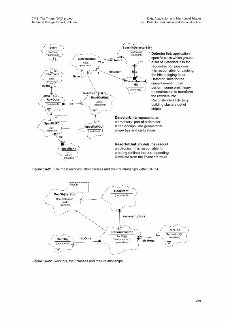
CMS: The Trigger/DAQ project Data Acquisition and High-Level TriggerTechnical Design Report, Volume II 14 Detector Simulation and Reconstruction
Figure 14-21 The main reconstruction classes and their relationships within ORCA.
Figure 14-22 RecObjs, their classes and their relationships.
data 0..n
A
RawData{persistent}
event 1
1
EventrawData() {persistent}
1RawEvent
data(){persistent}
0..n
1
1
1
Detector1..n
A
DetectorUnitdata()
{persistent}
ReadOut 1..n
A
ReadOutUnitdata()
{persistent}rou
1
1..n
1..n
Hit
SpecificRDfind()
{persistent}
SpecificHitid( )
value() {transient}
hit1
0..n
Hit
SpecificROU{persistent}
SpecificDetectorSetnewEvent( ){transient}
detectors 11..n
ReconstructedHit
{transient}
hits
1
0
detector1
DetectorSet: application-specific class which groups a set of DetectorUnits for reconstruction purposes. It is responsible for caching the hits beloging to its Detector Units for the current event. It can perform some preliminary reconstruction to transform the rawdata into Reconstructed Hits (e.g. building clusters out of strips)
DetectorUnit: represents an elementary part of a detector. It can encapsulate geometrical properties and calibrations.
ReadOutUnit: models the readout electronics. It is responsible for creating (online) the corresponding RawData from the Event structure.
ReconstructorRecObj()
Reconstructor() {persistent}
A
RecObj{persistent}
RecObj
RecObjIteratorRecObjIterator()
next() {transient}
RecEvent{persistent}
recObjs10..n
reconstructors1
0..n
A
RecUnitReconstruct()
{transient}strategy
0..n 1
249

CMS: The Trigger/DAQ project Data Acquisition and High-Level TriggerTechnical Design Report, Volume II 14 Detector Simulation and Reconstruction
14.3.2.1 Tracker Data and Local Reconstruction
14.3.2.1.1 Tracker Readout
In the pixel system, each barrel module is read out by 16 readout chips. In the end-cap modules, thenumber of readout chips varies from 2 to 10. Each readout chip reads an array of 52×53 pixels. The read-out is column oriented and therefore the chip is divided into 26 double columns 2×53 pixels each. Duringthe readout, all pixels with collected charge above a preset threshold are read and stored in data buffersplaced in column peripheries. Only pixels confirmed by the Level-1 Trigger are sent from the data buffersto the Front-End Drivers (FEDs) through analogue fibre links. A maximum of 36 links can be attached toa single FED. The whole readout system will consist of 38 FEDs (32 for the barrel and 6 for theend-caps). The FEDs will digitize the incoming data, build events, check for errors and transmit eventpackets to the DAQ.
In the microstrip system, signals produced by the silicon strip detectors are initially processed by thefront-end APV chips [14-16], each of which provides analogue readout of 128 silicon strips. The APVsamplify the signals and store them in an analogue memory pipeline until the Level-1 Trigger decision ismade. If this decision is positive, the data from multiplexed pairs of APVs are transmitted along analogueoptical fibre links to the Front-End-Driver (FED) cards [14-24] in the counting room. Each FED can proc-ess data from up to 192 APVs. The FEDs digitize the data, optionally perform zero-suppression and thensend them to the DAQ system.
14.3.2.1.2 Tracker Zero-suppression and Calibration
The zero-suppression and calibration procedures are different in the pixel and microstrip systems.
For the pixels, zero-suppression, i.e. the rejection of pixels without a significant signal, is performed bythe readout chip as described above. The following calibration measurements will be performed:
• measurement of the gains and pedestals (using injected charges),
• measurement of noise and threshold (using injected charges),
• average pixel counting rate/occupancy.
The first two will be carried out about twice per day in the ‘‘off-beam’’ periods. Neither the central DAQnor the global trigger system will be needed to perform these measurements. The last item is part of thedata monitoring procedure executed by the local pixel control system during standard data taking. It doesnot involve any special procedures and no special triggers are needed. A single calibration sequence gen-erates about 1.2 GB of data. In order to reduce the storage required, the full calibration data will be storedonce per week, and subsequently only changes in the values will be stored.
In the microstrip system, during normal physics running (both in p-p and Pb-Pb collisions) the FEDs op-erate in zero-suppression mode, since this significantly reduces the data volume. In this mode, the FEDsfirst subtract the pedestal and common-mode offsets from the signal on each strip, and then they searchfor clusters. Only strips associated to clusters have their pulse height information transmitted to the DAQ.It is proposed to estimate the common-mode offsets in each event from the median of the 128 pedes-tal-subtracted pulse heights on each APV. The clustering will be done by accepting groups of two or moreneighbouring strips, if they contain signals exceeding a threshold of a few times the noise, or isolatedstrips if they have a signal exceeding a higher threshold. The algorithms proposed for the common-modesubtraction and cluster finding have been evaluated using the ORCA Monte Carlo simulation. In p-p col-lisions, they are expected to give almost no loss in signal efficiency, whilst a small loss might be expected
250

CMS: The Trigger/DAQ project Data Acquisition and High-Level TriggerTechnical Design Report, Volume II 14 Detector Simulation and Reconstruction
in Pb-Pb collisions due to the very high occupancy. To accommodate any unpleasant surprises that actualLHC running conditions may show, the thresholds used for cluster finding are fully programmable. Fur-thermore, the FED algorithms are implemented in FPGA chips, which allows them (with some designwork) to be modified should this prove necessary.
The estimates of the pedestal and noise values for each strip, required by the FED for performing ze-ro-suppression, will be made by the FED VME crate controller. This will be done using a few thousandevents of raw data (i.e., not zero-suppressed) taken between fills. The choice of calibration algorithm isstill under study. However, preliminary estimates indicate that this calibration should take no more than afew minutes. The calibration constants will be monitored during physics fills by sampling the raw data ofa small fraction of events over VME.
14.3.2.1.3 Tracker Data Format and Data Rates
The data rates from the silicon pixel and microstrip trackers have been estimated for both high(1034 cm-2s-1) and low (2×1033 cm-2s-1) luminosity pp collisions, assuming a Level-1 Trigger rate of100 kHz, and also for Pb-Pb collisions, assuming a Level-1 Trigger rate of 7.6 kHz. The data rate is pro-portional to the pixel (strip) occupancy in events passing the Level-1 Trigger, where the occupancy is de-fined as the fraction of pixels (strips) accepted by the zero-suppression algorithm of the pixel readout chip(silicon-strip FED). This occupancy has been evaluated using ORCA.
In high luminosity p-p collisions, the tracker occupancy is dominated by the 17.5 superimposed mini-mum-bias events at each beam crossing. The uncertainty on the occupancy is estimated to be at least±35% and is dominated by the uncertainty (±30%) on the minimum-bias cross section. However, it alsoincludes contributions of ±12% from the uncertainty in the charged particle multiplicity and transversemomentum spectrum, and of ±12% due to the contribution of the ‘signal’ event which caused the Level-1Trigger to fire. (Monte Carlo studies of these signal events remain preliminary). At low luminosity, thereare five times fewer superimposed minimum-bias events per bunch crossing, so the signal event makes asignificant contribution to the occupancy. This increases the relative uncertainty on the low luminosityoccupancy to at least ±60%. These figures, described in detail in reference [14-25], are directly translatedto uncertainties on the data rates. Additional, subdetector-specific uncertainties are considered below.
In the pixel system, each FED will send to the DAQ a data packet starting with the standard packet header(two 32 bit words) and ending with the standard packet trailer (one 32 bit word). The header includes a bitfield identifying uniquely the FED. Each pixel will occupy a 32 bit word. The bit assignment is:
• 6 bit link address within the FED;
• 5 bit ROC address within the link;
• 5 bit double-column address within the ROC;
• 8 bit pixel address within the double-column;
• 8 bit analog signal.
Based on this assignment the FED data volume in bytes is calculated as 4⋅(3+number-of-pixels).
For the high (low) luminosity pp collisions, the pixel data volume for the barrel FEDs will be around2.0 (0.6) kB per event. For a 100 kHz trigger rate this corresponds to a maximum data rate of200 (60) MB/s. For the end-caps the data volume per FED will be smaller, about 1.8 (0.55) kB per event,corresponding to 180 (55) MB/s.
251

CMS: The Trigger/DAQ project Data Acquisition and High-Level TriggerTechnical Design Report, Volume II 14 Detector Simulation and Reconstruction
For Pb-Pb collisions the pixel occupancy is about ~14 times larger compared to that in pp collisions athigh luminosity. The resulting data volume per barrel FED is about 20 kB if the first barrel layer is usedand 12 kB without it (note that in [14-26] the first barrel layer was not considered). The maximum triggerrate given by the 200 MB/s limit will be 10 kHz (17 kHz) for the case with (without) the first layer.
For the microstrip tracker, detailed studies of the occupancies and data rates are presented in [14-25]. Insummary, the occupancy in high-luminosity pp collisions rises from 0.6% in the outermost barrel layer to2.8% in the innermost one. It has little dependence on the z coordinate, except in the outermost disks ofthe end-cap, where it increases by a factor of two, as a result of soft neutrons emitted from the ECALend-cap. The uncertainty on the occupancy is dominated by the physics effects mentioned above. Addi-tional contributions arising from uncertainties on the cross-talk between neighbouring strips and time res-olution of the electronics have been evaluated and are not significant. However, one potentially largesource of systematic uncertainty has yet to be evaluated and therefore represents a possible risk — the oc-cupancy in the outermost disks of the end-cap is dominated by soft neutron emission from the ECALend-cap. When the neutrons are captured, they yield soft photons, which create signals in the silicon. Ifthis results in a large rate increase one could envisage doubling the number of FEDs in the affected regionof the tracker to deal with it.
In the case of Pb-Pb collisions, the occupancy is about eight times higher than in high luminosity p-p col-lisions, but the corresponding strip tracker data volume is such that the desired Level-1 Trigger rate of7.6 kHz can be reached [14-25]. Even in the pessimistic scenario, where the true occupancy turns out tobe much higher, a minimum Level-1 Trigger rate of 3.4 kHz is guaranteed. At this trigger rate the DAQcan read out all of the tracker strips.
The data rate per FED depends on the tracker region which is read out. A preliminary allocation of striptracker detector modules to FEDs can be found in reference [14-25] and has been used to estimate thestrip tracker FED data rates. The data rate has a small dependence on the data format. In zero-suppressionmode, the strip tracker data produced by each FED for each event consists of a 112 B header followed, foreach pair of APVs, by a list of the reconstructed clusters they contain. For each cluster the following in-formation is given: the strip address of the first strip in the cluster, the cluster width in strips, and the pulseheight on each strip in the cluster. This format [14-24] has been assumed in estimating the data rates.
Figure 14-23 shows the estimated data rates per FED in the barrel and end-cap of the strip tracker, respec-tively. They take their highest value in high luminosity p-p collisions, where they rise to 104 MB/s in theoutermost disk of the end-cap. This rate is comfortably below the 200 MB/s limit that the DAQ can ac-cept. However, the strip tracker requires a total of 440 FEDs, whereas only about 256 of the DAQ switchinputs are available to it. It is therefore proposed to merge the data from pairs of FEDs reading the less oc-cupied parts of the tracker, using the DAQ Front-end Readout Links (FRL). A proposed scheme for doing
Figure 14-23 Data rate per FED in the strip tracker barrel (left) and end-caps (right).
252

CMS: The Trigger/DAQ project Data Acquisition and High-Level TriggerTechnical Design Report, Volume II 14 Detector Simulation and Reconstruction
this [14-25] reduces the number of switch inputs required to 272, with the maximum data rate per FRLbeing 138 MB/s.
The data rate is expected to fluctuate from event to event. In p-p collisions, the relative size of these fluc-tuations is, to a fair approximation, given by the relative fluctuation due to Poisson statistics in the expect-ed number of superimposed minimum-bias events per bunch crossing, i.e. 17.5±4.2 at high luminosityand 3.5±1.9 at low luminosity.
14.3.2.1.4 Tracker Reconstruction
The momentum reconstruction in CMS uses of a 4 T magnetic field provided by a super-conducting sole-noid magnet [14-27]. This high magnetic field affects event topologies, by confining low-PT chargedtracks to helical trajectories with small radius. Together with the steeply falling PT spectrum of chargedparticles in minimum-bias events, this results in the track density decreasing rapidly with increasing radi-us. Moreover, interesting physics events are characterized by tracks with PT exceeding 1 GeV; it is there-fore natural to attempt the reconstruction only of the tracks with PT higher than a given threshold in theGeV range. Momentum reconstruction within the rapidity range of |η|<1.6 benefits from the full momen-tum analysing power.
14.3.2.1.5 Cluster Reconstruction
The cluster reconstruction algorithm for the pixel detector starts from a cluster seed, defined as a pixelwith a signal to noise ratio S/N > 6. It then adds pixels adjacent to the cluster, if they have S/N > 5, contin-uing this process until no more adjacent pixels are found. Diagonally adjacent pixels are considered adja-cent. Finally the cluster is retained if its total charge has S/N > 10.1. The same algorithm is applied to thebarrel and forward pixel detectors.
The position of selected clusters is estimated independently in both dimensions. The position assignmentis based on the charge widths W, which are the projections onto the two directions of the area where thecharge is collected on the detector surface. In the transverse direction, both the track inclination and theLorentz shift contribute to the charge sharing. For clusters of two pixels the hit position is assigned as
where xcenter is the geometrical centre of the cluster and Q1 and Q2 are the charges deposited in the firstand last pixel hit respectively. This formula can be generalised for clusters larger than two pixels [14-28].
A precise charge width calculation is performed if the impact angles of the particle on the detector areknown from the partial track reconstruction, otherwise the track impact angles are estimated from the po-lar and azimuthal angles of the hit modules with all tracks assumed to come from the nominal interactionpoint.
The hit resolution depends also on the cluster size and the track impact angle. The pixel cluster size in thetransverse direction is mainly determined by the Lorentz shift and is usually 2 over the whole rapidityrange (in 82% of cases for high transverse momentum muon tracks). The cluster size in the longitudinalcoordinate is determined by the track impact angle and ranges from 1 to 6 pixels depending on the rapidi-ty. The error on the reconstructed position is estimated from the spatial displacement between simulatedand reconstructed hits (residuals) and error parameterization is performed as a function of the cluster sizeand the rapidity. An additional and more precise error parameterization is performed when the track im-
xcluster xcenter
Q2 Q– 1
2 Q1 Q2 )+(----------------------------+ W⋅=
253

CMS: The Trigger/DAQ project Data Acquisition and High-Level TriggerTechnical Design Report, Volume II 14 Detector Simulation and Reconstruction
pact angles are available from the partial or complete track reconstruction. A detailed description of theerror and position assignment of pixel hits can be found in [14-28].
The reconstruction inefficiency is defined as the fraction of simulated hits which do not have any associ-ated reconstructed hit. For the pixel detectors this is about 0.5%. The fraction of reconstructed hits whichare not associated to any simulated hit (ghost hits) is less than 0.01%. Both the reconstruction efficiencyand the ghost rate quoted here do not take into account readout inefficiencies.
Figure 14-24 shows the residuals and the pulls of the barrel detector hits. Typical pixel resolutions arearound 10 µm and the pulls are close to 1.
In the microstrip subsystem, the cluster reconstruction algorithm searches for strips with charge signifi-cance satisfying S(i)/N>3, where N is the average strip noise and S(i) the strip signal, both expressed inADC counts. Once at least one such strip is found, all adjacent strips with S(j)/N>2 are added to the clus-ter. When no adjacent strips above this threshold remain, the cluster charge Scluster is computed as the sumof the pulse heights over the accepted strips. If the condition Scluster/Ncluster> 5 is satisfied, the cluster isretained. The same algorithm is applied to both barrel and forward microstrip detectors. For isolatedstrips, which do not have adjacent strips over threshold, a stronger cut of S(i)/N>5 is imposed.
If the cluster size is less than 4, the cluster finder computes the cluster coordinate from the average posi-tion of all the strips assigned to the cluster, weighted by their pulse heights (this is the “centroid algo-rithm”). For wider clusters, Landau fluctuations spoil the resolution of this method, and only the twostrips at the edges of the cluster are used. The expected error on the measured position is estimated bylooking at the strip coverage by the simulated hits, using a simple parameterization. For double-sided(twin) detectors the stereo coordinates are calculated as well as their covariance term with the precise co-ordinate.
The reconstruction inefficiency is defined as the fraction of simulated hits, which do not result in recon-structed hits. This can be due to negative noise fluctuations, or to Landau fluctuations. In all the siliconmicrostrip detectors, it is estimated to be less than 0.5%.
The fraction of ghost reconstructed hits, which are not associated to any simulated hit, but are simply dueto noise fluctuations, is low because of the tight cut applied on the cluster significance. The fraction issimilar for barrel and end-cap detectors, and is estimated to be less than 0.1%.
Figure 14-24 shows, as an example, the residuals in silicon microstrip barrel detectors. The residual is de-fined as the distance, in µm, between the simulated and the reconstructed hit positions. The resolutionsdepend on whether the detectors have 512 or 768 strips, and on the detector shape and pitch. The widthsof the pulls are always close to 1.
Several effects are not yet correctly simulated in the present software. For example, the cluster inefficien-cy just reported is only “algorithmic”, and does not take into account the number of dead strips which canbe accepted when testing the modules (up to 2%). In the presence of dead strips, the cluster finder shouldbe improved to handle holes in clusters and to correctly calculate a clusters total signal and noise.
14.3.2.2 ECAL Data and Local Reconstruction
14.3.2.2.1 ECAL Crystal Readout
The shape of the signals coming out of the front-end amplifiers attached to the crystal photodetectors(APDs or VPTs) is shown in Figure 14-25. This signal is sampled and digitized at 40MHz. After the first
254
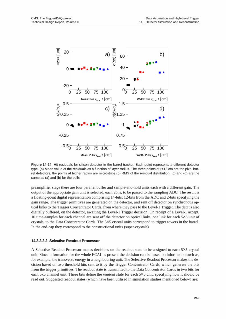
CMS: The Trigger/DAQ project Data Acquisition and High-Level TriggerTechnical Design Report, Volume II 14 Detector Simulation and Reconstruction
preamplifier stage there are four parallel buffer and sample-and-hold units each with a different gain. Theoutput of the appropriate gain unit is selected, each 25ns, to be passed to the sampling ADC. The result isa floating-point digital representation comprising 14-bits: 12-bits from the ADC and 2-bits specifying thegain range. The trigger primitives are generated on the detector, and sent off detector on synchronous op-tical links to the Trigger Concentrator Cards, from where they pass to the Level-1 Trigger. The data is alsodigitally buffered, on the detector, awaiting the Level-1 Trigger decision. On receipt of a Level-1 accept,10 time-samples for each channel are sent off the detector on optical links, one link for each 5×5 unit ofcrystals, to the Data Concentrator Cards. The 5×5 crystal units correspond to trigger towers in the barrel.In the end-cap they correspond to the constructional units (super-crystals).
14.3.2.2.2 Selective Readout Processor
A Selective Readout Processor makes decisions on the readout state to be assigned to each 5×5 crystalunit. Since information for the whole ECAL is present the decision can be based on information such as,for example, the transverse energy in a neighbouring unit. The Selective Readout Processor makes the de-cision based on two threshold bits sent to it by the Trigger Concentrator Cards, which generate the bitsfrom the trigger primitives. The readout state is transmitted to the Data Concentrator Cards in two bits foreach 5x5 channel unit. These bits define the readout state for each 5×5 unit, specifying how it should beread out. Suggested readout states (which have been utilised in simulation studies mentioned below) are:
Figure 14-24 Hit residuals for silicon detector in the barrel tracker. Each point represents a different detectortype. (a) Mean value of the residuals as a function of layer radius. The three points at r<12 cm are the pixel bar-rel detectors, the points at higher radius are microstrips (b) RMS of the residual distribution. (c) and (d) are thesame as (a) and (b) for the pulls.
-20
0
20
0 25 50 75 100
Mean: Res xlocal r [cm]
<∆x>
[µm
]
Mean: Res xlocal
0
20
40
60
0 25 50 75 100
Width: Res xlocal r [cm]
σ(∆x
) [µ
m]
Width: Res xlocal
-0.5
-0.25
0
0.25
0.5
0 25 50 75 100
Mean: Pulls xlocal r [cm]
<∆x/
σ x>
Mean: Pulls xlocal
0.5
0.75
1
1.25
1.5
0 25 50 75 100
Width: Pulls xlocal r [cm]
σ(∆x
/σx)
Width: Pulls xlocal
a) b)
c) d)
255
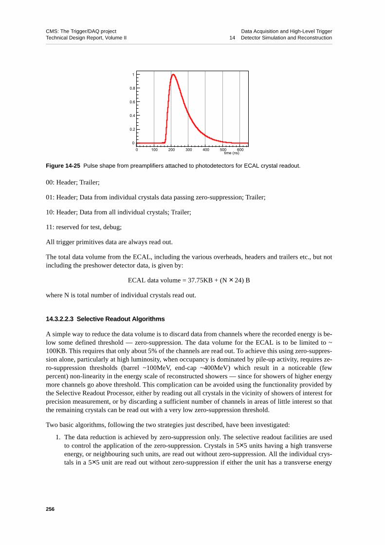
CMS: The Trigger/DAQ project Data Acquisition and High-Level TriggerTechnical Design Report, Volume II 14 Detector Simulation and Reconstruction
00: Header; Trailer;
01: Header; Data from individual crystals data passing zero-suppression; Trailer;
10: Header; Data from all individual crystals; Trailer;
11: reserved for test, debug;
All trigger primitives data are always read out.
The total data volume from the ECAL, including the various overheads, headers and trailers etc., but notincluding the preshower detector data, is given by:
ECAL data volume = 37.75KB + (N × 24) B
where N is total number of individual crystals read out.
14.3.2.2.3 Selective Readout Algorithms
A simple way to reduce the data volume is to discard data from channels where the recorded energy is be-low some defined threshold — zero-suppression. The data volume for the ECAL is to be limited to ~100KB. This requires that only about 5% of the channels are read out. To achieve this using zero-suppres-sion alone, particularly at high luminosity, when occupancy is dominated by pile-up activity, requires ze-ro-suppression thresholds (barrel ~100MeV, end-cap ~400MeV) which result in a noticeable (fewpercent) non-linearity in the energy scale of reconstructed showers — since for showers of higher energymore channels go above threshold. This complication can be avoided using the functionality provided bythe Selective Readout Processor, either by reading out all crystals in the vicinity of showers of interest forprecision measurement, or by discarding a sufficient number of channels in areas of little interest so thatthe remaining crystals can be read out with a very low zero-suppression threshold.
Two basic algorithms, following the two strategies just described, have been investigated:
1. The data reduction is achieved by zero-suppression only. The selective readout facilities are usedto control the application of the zero-suppression. Crystals in 5×5 units having a high transverseenergy, or neighbouring such units, are read out without zero-suppression. All the individual crys-tals in a 5×5 unit are read out without zero-suppression if either the unit has a transverse energy
Figure 14-25 Pulse shape from preamplifiers attached to photodetectors for ECAL crystal readout.
time (ns)0 100 200 300 400 500 600
0
0.2
0.4
0.6
0.8
1
256

CMS: The Trigger/DAQ project Data Acquisition and High-Level TriggerTechnical Design Report, Volume II 14 Detector Simulation and Reconstruction
greater than a first (low) threshold, or a neighbouring unit has an transverse energy above a second(higher) threshold.
2. Some data reduction is obtained by applying zero-suppression at a fairly modest threshold to allchannels. Further data reduction is obtained by not reading out any individual crystals in some 5×5units. The individual crystals in a 5×5 unit are read out if either the unit has a transverse energygreater than a first (low) threshold, or a neighbouring unit has an transverse energy above a second(higher) threshold.
Using these algorithms the ECAL data volume can be reduced to the 100 kB target with negligible impacton physics. Figure 14-26 shows the distribution of ECAL data volume for jet events when an algorithm ofthe first type listed above is used. The simulation was made using fully simulated high-ET jet events withpile-up corresponding to a) 2×1033 cm-2s-1, and b) 1034 cm-2s-1. At high luminosity, for energies greaterthan about twice the electronics noise width, the occupancy is completely dominated by pile-up. The sim-ulation was done with a model of the readout, where, in the end-caps, the units are trigger towers ratherthan super-crystals. The parameters of the algorithm used in this example are such that all channels be-longing to trigger towers having ET > 2.5 GeV are read out, as well as all channels in trigger towersneighbouring towers with ET > 5 GeV. The remaining towers are readout with a zero-suppression thresh-old of 120 MeV in the barrel and 450 MeV in the end-cap.
The algorithms described give some freedom and flexibility to tune the ECAL data volume. Figure 14-27shows how the mean ECAL data volume for high-ET jet events at 1034 cm-2s-1 varies as a function of thezero-suppression threshold for three different pairs of values for the thresholds at which all crystals areread out from a tower (‘Single’) or from all neighbouring towers (‘Centre’).
14.3.2.2.4 Preshower Data
The CMS ECAL also includes the preshower detectors, on the end-caps, comprising 4304×32 siliconstrips. Time samples, at 40 MHz, are stored in an analogue buffer on the detector. On receipt of a Level-1Trigger three time samples per strip are digitized at 20 MHz, using the same 12-bit ADC as for the ECALcrystals, and transferred, by optical links, off the detector to the upper level readout system. A total of
Figure 14-26 Distribution of ECAL data volume for jet events at a) 2x1033 cm-2s-1, and b) 1034 cm-2s-1.
0
50
100
20 40 60 80 100 120 140Data Volume, KB
Even
ts
SR (Scheme 1)
2x1033 Pileup
Center: 5.0 GeV
Single: 2.5 GeV
Barrel: 120 MeV
Endcap: 450 MeV
Mean: 59 KB
Sigma: 10 KB
0
50
100
150
60 80 100 120 140 160 180 200Data Volume, KB
Even
ts
SR (Scheme 1)
1034 Pileup
Center: 5.0 GeV
Single: 2.5 GeV
Barrel: 120 MeV
Endcap: 450 MeV
Mean: 97 KB
Sigma: 14 KB
257

CMS: The Trigger/DAQ project Data Acquisition and High-Level TriggerTechnical Design Report, Volume II 14 Detector Simulation and Reconstruction
4304×148 bytes are transferred. In the upper level readout system the data is zero-suppressed at a levelmuch greater than the electronics noise width — 3σnoise is suggested (this is about equal to 60% of thesignal given by a minimum ionizing particle). Average occupancy at high luminosity is about 2%. Thus alittle more than 10 kB of data will be finally read out from the preshower detector.
14.3.2.2.5 Reconstruction of the Energy from the Time Frames
The first step in reconstructing the energy deposited in a crystal from the time frames of ten time samplesis the expansion of the floating point representation by multiplying the 12-bit ‘mantissa’ by the appropri-ate gain specified by the 2-bit ‘exponent’. At this point, also, account must be taken of the difference inpedestal between the ranges. The energy deposited in the crystal is then reconstructed by a scalar productbetween a vector of time samples and a vector of weights, to give a single value proportional to the depos-ited energy. The reconstruction currently used with simulated data uses only 8 of the time samples — 3before the pulse, and 5 in the pulse. The precise details of the algorithm to be used and the methods of ex-tracting the optimum weights are currently under study, and their fine tuning will require test beam datataken with the final front-end electronics.
The time of the signal, as well as the energy, can be reconstructed from the time frames. This can proba-bly best be done using another vector of weights, optimized for extracting the pulse time rather than itsmagnitude. In the present simulation work a simple χ2 is constructed to measure how well the observedpulse conforms to the hypothesis that the pulse was generated by energy deposited in the bunch crossingof the trigger event. Currently the only use that is made of this χ2 is to suppress out-of-time clusters whenmaking ECAL isolation cuts.
The reconstruction of the preshower signal is both simpler (there is a single gain range and only threetime samples) and less critical, but it is likely to use similar techniques.
Figure 14-27 Mean ECAL data volume for high ET jet events at 1034 cm-2s-1 as a function of the zero-suppres-sion threshold. The three curves correspond to different tower thresholds for removal of the zero-suppression(see text).
50
75
100
125
150
1.5 2 2.5 3 3.5 4 4.5 5Sigma suppression
Eve
nt
Dat
a V
olu
me
[KB
] Center - 5.0, Single - 2.5Center - 10.0, Single - 5.0Center - 20.0, Single - 10.0
(SR Scheme 1)
258

CMS: The Trigger/DAQ project Data Acquisition and High-Level TriggerTechnical Design Report, Volume II 14 Detector Simulation and Reconstruction
14.3.2.3 HCAL Data and Local Reconstruction
14.3.2.3.1 HCAL Readout
The data output by the QIE are in a pseudo-floating point format, with 5 bits of mantissa, 2 bits of range,and two bits for capacitor identification. The pedestal is set in the sixth ADC bin, and is assumed to havebeen measured to high precision during the abort gap.
The QIE data is processed to make trigger primitives for Level-1 and held, to be sent to the DAQ on re-ceipt of a Level-1 accept. To produce the Level-1 Trigger primitives, the time samples are first convertedfrom energy to transverse energy. If there is more than one depth segment (excluding the HO), as is thecase for all towers beyond tower 15, the depth segments are summed. In the HF, the 2 readouts (long andshort fibers) are summed, and the HF towers are given a coarser segmentation by ganging together 2 in φby 3 in η of the full readout segmentation. The signal shape from the HB/HE/HO is longer than the timebetween bunch crossings, and several time samples are used to estimate the energy.
The algorithm used to extract the transverse energy from the time samples in the HB/HE/HO is simple.The amplitudes from two consecutive beam crossings are summed and the pedestal subtracted. The am-plitude is then multiplied by a calibration factor (1.11) which includes a correction for the fraction of thesignal outside the two time buckets. In the simulation we assume 0.68 MeV/pe in the HB, 0.45 MeV/pe inthe HE, and 0.25 MeV/pe in the HO, with sampling fractions of 220 in the HB, and 147 in the HE. Thesemultiplicative corrections will be implemented using a programmable look-up table in hardware.
The pattern of energy deposits in the different time samples is checked to verify its association with thetriggering crossing. If the signal calculated from the time samples as described above, assuming the ener-gy comes from the current crossing, is bigger than that calculated assuming the energy comes from theprevious or subsequent crossing, the energy is kept. Otherwise, it is zeroed. The trigger primitives arethen sent, in a compressed format with a LSB of 1 GeV, to the Level-1 regional calorimeter trigger.
The algorithm in the HF is very simple. The energy in one time sample is converted to GeV after pedestalsubtraction. Since the pulse is much shorter than one beam crossing, there is no problem with out-of-timeenergy.
14.3.2.3.2 HCAL Zero-suppression and Data Rates
The HCAL readout contains a header and trailer, trigger primitive data, and precision readout (DAQ path)data. The header/trailer information consists of approximately 160 service bits per Data ConcentratorCard (DCC). There are 32 DCC’s. An additional few words of service bits (a few ×16 bits) is also needed.A total of 4320 channels of trigger primitive data, 9 bits per channel, are read out. The full-precision rawdata for the DAQ path is checked to see if it is above a zero-suppression threshold. Currently, this thresh-old is assumed to be 500 MeV in energy in the HB/HE/HF and 150 MeV in the HO. If the energy is abovethreshold, ten time samples of QIE data are read out, otherwise a single time sample is read out.
There are 7560 channels in the HB/HE/HF and 2160 in the HO. When address bits and other service in-formation are included there are 16 bits per time sample. Table 14-4 shows an example of a possible dataformat.
The HCAL data volume per readout is therefore given by
NDCCH L D O+ HBEFNHBEF P NR+( ) OHONHO P A NR+ +( )+ + +
259

CMS: The Trigger/DAQ project Data Acquisition and High-Level TriggerTechnical Design Report, Volume II 14 Detector Simulation and Reconstruction
where NDCC is the number of DCC’s, H is the header and trailer information (=2×16+160=192 bits), L isthe trigger primitive data (9×4320=38880 bits), D is the 7 bits of QIE data per HB/HE/HF channel(8×7560=60480) which is read out regardless of whether the channel is over threshold or not, P is thenumber of bits used for the pedestal value (8), R is the number of bits used for the ADC and service words(16), N is the number of time samples (10), NHBEF is the number of HB/HE/HF readout channels (7560),NHO is the number of HO readout channels (2160), OHBEF is the probability for an HB/HE/HF to be overthe zero-suppression threshold and OHO is the same probability for the HO.
Figure 14-28 shows the occupancy as a function of the zero-suppression threshold in ET/(∆η×∆φ) nor-malized to the size of a central HB tower, in minimum-bias events at high luminosity for the shorter of thetwo possible HCAL signal shapes. It is currently planned to run with a readout threshold ofET=500 MeV/(0.087×0.087), which gives an occupancy of about 10% for the HB/HE/HF, roughly inde-pendent of η. The HO will have a lower threshold, around 150 MeV, and has an occupancy there of about5%. The total HCAL data volume at high luminosity will be
Since the Level-1 Trigger operates at up to 100 kHz, and the total data rate is 245 kb per Level-1 Trigger,the total required readout throughput is 24 Gb/s. This data rate is consistent with the hardware bandwidth:each DCC sustains 200 MB/s, i.e. the 32 DCC’s sustain 6400 MB/s or 57 Gb/s.
Table 14-4 Tentative HCAL Data Format.
word type Byte 3 Byte 2 Byte 1 Byte 0
HEADER EV #23-16 EV # 15-8 Zeros EV #7-0
EXT HEADER 2 No. Trig Towers HTR card # Spare + BX#11-8 BX#7-0
EXT HEADER 3 Spare Spare Trigger type ORBIT #
Trig Towers 24-21 Tower 24 Tower 23 Tower 22 Tower 21
Trig Towers 20-17
Trig Towers 16-13
Trig Towers 12-9
Trig Towers 8-5
Trig Towers 4-1 Tower 4 Tower 3 Tower 2 Tower 1
Trigger Muon bits Muon bits 24-1
DAQ Mask Mask for each of the 24 Channels of DAQ Data
DAQ Data Data Data
DAQ Data, cont Data Data
FE Link Errors
CapID Errors
Other Errors
TRAILER EV # 7-0 zeros
32 192× 38880 60480 0.1( ) 7560( ) 8 10 16×+( ) 0.05( ) 2160( ) 8 10 16×+( )+ + + + 245kb=
260
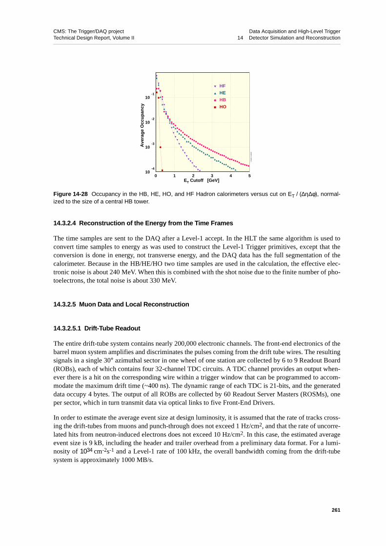
CMS: The Trigger/DAQ project Data Acquisition and High-Level TriggerTechnical Design Report, Volume II 14 Detector Simulation and Reconstruction
14.3.2.4 Reconstruction of the Energy from the Time Frames
The time samples are sent to the DAQ after a Level-1 accept. In the HLT the same algorithm is used toconvert time samples to energy as was used to construct the Level-1 Trigger primitives, except that theconversion is done in energy, not transverse energy, and the DAQ data has the full segmentation of thecalorimeter. Because in the HB/HE/HO two time samples are used in the calculation, the effective elec-tronic noise is about 240 MeV. When this is combined with the shot noise due to the finite number of pho-toelectrons, the total noise is about 330 MeV.
14.3.2.5 Muon Data and Local Reconstruction
14.3.2.5.1 Drift-Tube Readout
The entire drift-tube system contains nearly 200,000 electronic channels. The front-end electronics of thebarrel muon system amplifies and discriminates the pulses coming from the drift tube wires. The resultingsignals in a single 30° azimuthal sector in one wheel of one station are collected by 6 to 9 Readout Board(ROBs), each of which contains four 32-channel TDC circuits. A TDC channel provides an output when-ever there is a hit on the corresponding wire within a trigger window that can be programmed to accom-modate the maximum drift time (~400 ns). The dynamic range of each TDC is 21-bits, and the generateddata occupy 4 bytes. The output of all ROBs are collected by 60 Readout Server Masters (ROSMs), oneper sector, which in turn transmit data via optical links to five Front-End Drivers.
In order to estimate the average event size at design luminosity, it is assumed that the rate of tracks cross-ing the drift-tubes from muons and punch-through does not exceed 1 Hz/cm2, and that the rate of uncorre-lated hits from neutron-induced electrons does not exceed 10 Hz/cm2. In this case, the estimated averageevent size is 9 kB, including the header and trailer overhead from a preliminary data format. For a lumi-nosity of 1034 cm-2s-1 and a Level-1 rate of 100 kHz, the overall bandwidth coming from the drift-tubesystem is approximately 1000 MB/s.
Figure 14-28 Occupancy in the HB, HE, HO, and HF Hadron calorimeters versus cut on ET / (∆η∆φ), normal-ized to the size of a central HB tower.
10-4
10-3
10-2
10-1
0 1 2 3 4 5
■ HO
● HB
▲ HE
▼ HF
ET Cutoff [GeV]
Ave
rag
e O
ccu
pan
cy
S. A
bd
ulli
n 2
1/10
/200
2
261
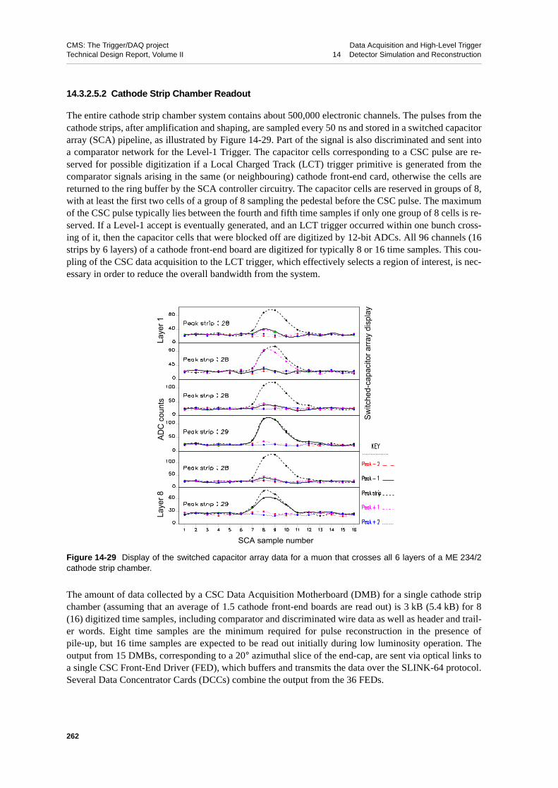
CMS: The Trigger/DAQ project Data Acquisition and High-Level TriggerTechnical Design Report, Volume II 14 Detector Simulation and Reconstruction
14.3.2.5.2 Cathode Strip Chamber Readout
The entire cathode strip chamber system contains about 500,000 electronic channels. The pulses from thecathode strips, after amplification and shaping, are sampled every 50 ns and stored in a switched capacitorarray (SCA) pipeline, as illustrated by Figure 14-29. Part of the signal is also discriminated and sent intoa comparator network for the Level-1 Trigger. The capacitor cells corresponding to a CSC pulse are re-served for possible digitization if a Local Charged Track (LCT) trigger primitive is generated from thecomparator signals arising in the same (or neighbouring) cathode front-end card, otherwise the cells arereturned to the ring buffer by the SCA controller circuitry. The capacitor cells are reserved in groups of 8,with at least the first two cells of a group of 8 sampling the pedestal before the CSC pulse. The maximumof the CSC pulse typically lies between the fourth and fifth time samples if only one group of 8 cells is re-served. If a Level-1 accept is eventually generated, and an LCT trigger occurred within one bunch cross-ing of it, then the capacitor cells that were blocked off are digitized by 12-bit ADCs. All 96 channels (16strips by 6 layers) of a cathode front-end board are digitized for typically 8 or 16 time samples. This cou-pling of the CSC data acquisition to the LCT trigger, which effectively selects a region of interest, is nec-essary in order to reduce the overall bandwidth from the system.
The amount of data collected by a CSC Data Acquisition Motherboard (DMB) for a single cathode stripchamber (assuming that an average of 1.5 cathode front-end boards are read out) is 3 kB (5.4 kB) for 8(16) digitized time samples, including comparator and discriminated wire data as well as header and trail-er words. Eight time samples are the minimum required for pulse reconstruction in the presence ofpile-up, but 16 time samples are expected to be read out initially during low luminosity operation. Theoutput from 15 DMBs, corresponding to a 20° azimuthal slice of the end-cap, are sent via optical links toa single CSC Front-End Driver (FED), which buffers and transmits the data over the SLINK-64 protocol.Several Data Concentrator Cards (DCCs) combine the output from the 36 FEDs.
Figure 14-29 Display of the switched capacitor array data for a muon that crosses all 6 layers of a ME 234/2cathode strip chamber.
Switc
hed-
capa
cito
r arra
y di
spla
y
Laye
r 1AD
C c
ount
sLa
yer 8
SCA sample number
262

CMS: The Trigger/DAQ project Data Acquisition and High-Level TriggerTechnical Design Report, Volume II 14 Detector Simulation and Reconstruction
A single muon that traverses four CSC stations in the end-cap generates 12 kB (22 kB) for 8 (16) timesamples, assuming no pile-up from other muons or punch-through. However, the average event size de-pends on the occupancy of the chambers as well as the fraction of triggers that contain muons. From sim-ulation, and assuming that half of all triggered events contain a muon, it is expected that the average CSCevent size is 10 kB. At low luminosity, this assumes that 16 time samples are read out, but to maintain thesame event size at high luminosity requires a reduction to 8 time samples as well as a tighter LCT require-ment (a coincidence of the anode and cathode LCT, rather than just cathode). At a luminosity of2×1033 cm-2s-1, the overall CSC bandwidth is approximately 500 MB/s with an Level-1 rate of 50 kHz,and at the design luminosity of 1034 cm-2s-1, it is approximately 1000 MB/s for a Level-1 rate of 100 kHz.
14.3.2.5.3 Resistive Plate Chamber Readout
The Resistive Plate Chamber muon system contains nearly 200,000 electronic channels. The pulses com-ing from the RPC strips are amplified and discriminated by an 8-channel ASIC on the front-end boards.All single strip data used as input to the RPC Pattern Comparator logic used by the Level-1 Trigger areread by the readout system. An “LMUX” zero-suppression scheme used by the link subsystem, describedin [14-35], guarantees that only non-empty channels are read. The data collected by the readout systemare delivered to standard Readout Dual-Port Memory (RDPM) modules. The occupancy of the RPC sys-tem is dominated by noise, and leads to an average event size of 600 bytes.
14.3.2.6 Track Segment Reconstruction
14.3.2.6.1 Track Segment Reconstruction in the Drift Tube System
The reconstructed position of a muon hit in a drift cell is determined from the corresponding TDC meas-urement and the effective drift velocity (also used in the creation of the hits in the simulation, parameter-ized as a function of the track direction and the magnetic field), which must be known to an accuracy ofabout 1% in order to obtain a position resolution of about 250 µm. The reconstruction is performed in twosteps: an average drift velocity is used for a first determination of the reconstructed hit position and direc-tion. Next, these parameters are used to determine the correct effective drift velocity to refine the hit re-construction. The final residuals of the simulated reconstructed hits in the r-φ bending plane and in the r-znon-bending plane have widths of 285 µm and 340 µm, respectively, for muons with 10<PT<100 GeV/cuniformly distributed throughout the barrel detector (and thus averaging over all inclination angles, cellpositions, and magnetic fields). It should be noted that in the r-φ plane tracks originating from promptmuons have angles up to 15° with respect to the direction normal to the chamber plane, while in the r-zplane, the inclination angle extends to about 50°, depending on η.
Track segments are created by performing simple least-squares fits of straight lines in two-dimensionsthrough the reconstructed hits in the superlayers of a chamber set. This is done separately in r-φ and r-z,but the 2-D segments are then associated into 3-D segments. Up to 12 points per track segment are includ-ed, corresponding to the maximum number of the chamber measurement layers in a station. Hit sharingbetween segments is not allowed, and left-right ambiguities are resolved on the basis of a χ2 criterion,with the additional constraint that the track originates from the interaction region for the r-z orientation.The position and direction of each track segment (after the reconstructed hit refinement) are input to theKalman filter algorithm for the track reconstruction used by the HLT. The residuals of the track segmentposition in the r-φ plane are considerably improved with respect to those obtained from a single drift-tubelayer, as shown in Figure 14-30a, which shows the overall simulated residual distribution from chambersin all DT wheels and stations. The central width of the distribution is 109 µm. The corresponding residu-als of the track segment direction angle in the r-φ plane (with up to 8 reconstructed hits and a 26 cm lever
263

CMS: The Trigger/DAQ project Data Acquisition and High-Level TriggerTechnical Design Report, Volume II 14 Detector Simulation and Reconstruction
arm) are shown in Figure 14-30b. The direction angle is defined with respect to the direction normal tothe chamber plane (z). This distribution has a central width of 0.9 mrad. In the r-z (non-bending) plane,the direction angle residuals vary from 9−13 mrad for |η|<0.9. For higher η values, corresponding totracks in the outer wheels of the MB1 and MB2 stations (see Fig. 14-10), the resolution in the non-bend-ing plane worsens to 35 mrad.
The corresponding position and direction errors are also determined for each track segment in order to beused by the Kalman filter algorithm. In all cases, Gaussian fits to the central part of this pull distributionhave zero mean and approximately unit width. However, long tails do exist, partially due to difficult re-gions at high η where a strong magnetic fringe field is present.
14.3.2.6.2 Cluster Finding and Track Segment Reconstruction in the Cathode Strip Chambers
The charge from a chamber hit is distributed across 3 to 5 cathode strips. In order to precisely reconstructthe position of the hit, one must accurately determine the pulse height on each strip from the SCA infor-mation and perform a fit to the expected spatial shape of the charge distribution. The measurement of thecharge of each strip is taken from the fifth SCA sample, which is constructed to be taken at the peak of thetime evolution of the signal that triggered the digitization. Baseline shifts are accounted for by subtractingfrom each pulse the average of the first two SCA samples, taken before the signal arrived. No correctionis made for signal pile-up.
Strip clusters are reconstructed starting from the strip with the maximum charge, and including the twoneighbouring strips. The so-called “Gatti function” [14-23] is used to fit the spatial distribution of thecharge over the 3-strip cluster (and is also used in the creation of the strip charge in the simulation). Withthis reconstruction, the fitted width of the central part of the residual distribution is about 240 µm in thesimulation of CSC layers from ME2, ΜΕ3, and ΜΕ4, as shown in Figure 14-31a. (It is about 120 µm forME 1/1.) The pull distribution of the reconstructed strip positions for the same chambers is shown inFigure 14-31b.
Reconstructed hits are created at each intersection of a cathode strip cluster with each wire group that hasenough charge to be digitized. The bunch crossing assignment between the anode and cathode clustersmust agree to within two bunch crossings. No attempt is made to cluster neighbouring wire groups or tosuppress ghost combinations.
Track segments are created by performing simple χ2 fits of straight lines through the reconstructed hits in3-D. Due to the small lever arm of the hits within a chamber, a fast straight line fit neglecting the small
Figure 14-30 Residuals in the r-φ plane of the DT track segment position (a), and the DT track segment direc-tion angle (b), defined with respect to the direction normal to the chamber.
�0.1 �0.05 0 0.05 0.1X0
rec � X0sim �cm�
200
400
600
800
Nr.
segm
ents
�a� Σ � 109 Μm
�7.5 �5 �2.5 0 2.5 5 7.5dx�dzrec � dx�dzsim �mrad�
200
400
600
800
Nr.
segm
ents
�b� Σ � .861mrad
264

CMS: The Trigger/DAQ project Data Acquisition and High-Level TriggerTechnical Design Report, Volume II 14 Detector Simulation and Reconstruction
curvature effect of the residual magnetic field inside the chambers is accurate enough for the Kalman fitthat will be performed using the segments. The procedure starts with the leftmost hit in the first layer of achamber and the rightmost hit of the sixth layer. One hit is added per layer, and the line fit is redone afterthe addition. A hit is replaced if a better match is found. Hits must match within 2.5 mm in φ, and χ2<100is required. A track segment must contain at least 4 of the 6 possible hits. Overall, the algorithm is 98%efficient for 50 GeV muons, with the inefficiency mainly arising from showers. The direction resolutionof the 3-D track segment varies from 7 to 11 mrad in φ and from 50 to 120 mrad in θ at 50 GeV, depend-ing on the CSC chamber type.
14.3.2.6.3 Cluster Reconstruction in the Resistive Plate Chambers
The clustering procedure applied to the strip signals from the RPC chambers consists of grouping all ad-jacent strips above a threshold. Once all groups are formed, the reconstructed position of each cluster istaken to be the centre-of-gravity of the total area covered by the cluster of strips. Thus, in the barrel, it issimply the centre of the rectangular area of strips; in the end-cap, it is the centre of a trapezoidal-shapedregion. The error on the reconstructed position along each axis is calculated assuming a uniform hit prob-ability across the cluster area; in other words, it is 1/√12 times the length of the corresponding side.
14.4 Global Reconstruction
14.4.1 Track Reconstruction
Due to the complexity of the CMS tracker, with its tens of thousands of detector modules, tens of millionsof channels, and tens of thousands of hits per bunch crossing, it is not obvious that there is a single opti-mal track reconstruction algorithm in all circumstances. It is more likely that there should be several spe-cific algorithms, each of them optimized for a specific task within the complex physics at CMS.
Figure 14-31 Simulated residuals (a) and pull distribution (b) of the reconstructed strip positions in the CSC lay-ers from ME2, ME3 and ME4.
/ ndf 2χ 1231 / 23
Constant 1.272e+04
Mean 0.0002398
Sigma 0.02302
(cm)φsim-xφ
recx-0.2 -0.15 -0.1 -0.05 -0 0.05 0.1 0.15 0.20
2000
4000
6000
8000
10000
12000
14000
/ ndf 2χ 1231 / 23
Constant 1.272e+04
Mean 0.0002398
Sigma 0.02302
Residuals ME2,ME3,ME4 / ndf 2χ 210.4 / 57
Constant 6310
Mean 0.01169
Sigma 1.238
φxσ) / φsim-xφ
rec (x-5 -4 -3 -2 -1 0 1 2 3 4 50
1000
2000
3000
4000
5000
6000
7000 / ndf 2χ 210.4 / 57
Constant 6310
Mean 0.01169
Sigma 1.238
Pull ME2,ME3,ME4
(a) (b)
265
CMS: The Trigger/DAQ project Data Acquisition and High-Level TriggerTechnical Design Report, Volume II 14 Detector Simulation and Reconstruction
Therefore a flexible framework for developing and evaluating track reconstruction algorithms is used[14-29].
The CMS track reconstruction framework is based on the Kalman Filter formalism [14-30], but not re-stricted to it. More advanced algorithms, like the Deterministic Annealing Filter or the Multi Track Filterhave been successfully implemented as well [14-29].
The mathematical complexity of track reconstruction and fitting limits the number of developers. Usuallythe algebra involved is localized in a few places and is largely independent of the various types of trackreconstruction algorithms. Therefore the development of track reconstruction algorithms can be madeeasier and more accessible if the algebra can be separated from the logic of the algorithm. In the case ofthe Kalman filter formalism, the basic operations are propagation of a trajectory state to some surface,and updating of a trajectory state with information from a measurement. They are encapsulated in two ba-sic components, the Propagator and the Updator.
These components, in collaboration with the detector geometry components, allow for simple and flexibleimplementation of the different stages of the track reconstruction described below.
14.4.1.1 Influence of Tracker Material on Track Reconstruction
Track reconstruction is based upon the equations of motion of a charged particle in a magnetic field. Inthe standard Kalman filter [14-30] they determine the evolution of the state vector and its covariance ma-trix. This simple model has to be modified in the presence of matter: deterministic effects are included inthe track model, stochastic processes result in additional contributions to the covariance matrix (“processnoise” in the terminology of dynamic systems).
In order to speed up the reconstruction, the material of the tracker is described in a simplified way:
• all material is assumed to be concentrated on thin surfaces. In the current version these surfaces co-incide with the active elements;
• the material properties of each detector layer are described by two numbers: the thickness in unitsof radiation length, and the thickness multiplied by the mean ratio of atomic number to atomicmass.
Two kinds of effects are taken into account:
• energy loss (for electrons due to Bremsstrahlung, for all other particles due to ionization), and
• multiple scattering.
Ionization energy loss is described according to the Bethe-Bloch formula without density correction[14-31]. The mean excitation energy used is that of silicon. The average and variance of the fractional en-ergy loss of electrons due to radiation are computed based on the p.d.f. given by Bethe and Heitler[14-32].
The effect of multiple scattering is calculated using the approximation for the Gaussian core given byHighland [14-31]. As explained above, the effects due to the presence of material only enter the propaga-tion stage of the Kalman filter. The track propagation is thus divided into two parts: a purely geometricalextrapolation and an update of track parameters and their covariance matrix at the destination surface.The mean energy loss <dE> results in a change of the predicted momentum, while the spread of the ener-gy loss and the deflection due to multiple scattering modify the covariance matrix. Corrections to the pathlength due to the angle of incidence are also taken into account and applied both in the forward and, re-verting the sign of <dE>, in the backward filter.
266

CMS: The Trigger/DAQ project Data Acquisition and High-Level TriggerTechnical Design Report, Volume II 14 Detector Simulation and Reconstruction
The simplified treatment of the material is valid only inside the tracker volume. Propagation to the Muonsystem requires detailed knowledge of the passive material. Currently the propagations outside of thetracker volume are performed with the GEANE package [14-33], which uses the full simulation geome-try. For convenience and conformance the GEANE routines are also encapsulated in a Propagator.
14.4.1.2 Track Reconstruction Phases
Track reconstruction is decomposed in four phases:
• Trajectory seed generation;
• Trajectory building - seeded pattern recognition;
• Trajectory cleaning - resolution of ambiguities;
• Trajectory smoothing - final fit.
These components are described in detail in the following sections.
14.4.1.2.1 Seed Generator
Seed generation, which provides initial trajectory candidates can be internal to the tracking detector (innertracker or muon system), or external, using input from other detectors (calorimeters). The seed must pro-vide initial trajectory parameters and errors. To constrain all five parameters of the trajectory one needs atleast two two-dimensional position measurements and a beam spot constraint, or a calorimetric measure-ment of position and energy and a beam spot constraint.
Consequently, internal seeds consist of pairs of RecHits and use a beam spot constraint and a minimaltransverse momentum constraint to provide initial trajectory parameters. The beam spot constraint mayintroduce a bias at this stage, which is removed during the final fit.
The “beam spot”, or track origin region, used in the seed generator, is chosen according to context. Forexample, to reconstruct primary muons when the event vertex is not known the origin can be a cylinderwith radius of 50 µm and length of 30 cm. If the primary vertex is known, e.g. from the already recon-structed muon, and the goal is b-jet tagging, the origin could be a cylinder 1 mm in radius and 2 mm long.The choice of the origin size can have dramatic effect on the reconstruction efficiency, fake rate, and CPUtime. If the origin is too small the track reconstruction efficiency will suffer; if the origin size is biggerthan the physics requirements, additional CPU time will be wasted to reconstruct ghost tracks that willhave to be removed with additional track selection criteria.
In a similar way, the choice of the minimal transverse momentum has a strong influence on the number ofseeds, and even more on the overall CPU time, since it takes longer to reconstruct a soft track than a hardtrack. The minimal transverse momentum is defined by physics requirements. It is typically 0.9 GeV forb-tagging, and can be as high as 20 GeV for trigger muon reconstruction.
The two hits that constitute an internal tracker seed are chosen to come from two different layers, the socalled seeding layers. The best reconstruction performance, both in efficiency, accuracy and CPU time, isachieved when the pixel layers are used for seeding. There are several reasons for this:
• the channel occupancy and the noise of the pixel detectors is much lower than for the strip detec-tors;
• the quality of the 2D measurement is much better for the pixel detectors: there are no combinatori-al ambiguities and both coordinates are measured with ~20 µm accuracy;
267

CMS: The Trigger/DAQ project Data Acquisition and High-Level TriggerTechnical Design Report, Volume II 14 Detector Simulation and Reconstruction
• the interaction probability for π in the tracker is so high that more than 20% of the 1 GeV pions donot reach the outermost layers. The reconstruction efficiency is therefore lower if the outer seedinglayers are used, even if one allows many combinations;
• the number of seeds is smaller for pixel layers (for a given origin size and minimal transverse mo-mentum);
• for some applications, like b-tagging or secondary vertex reconstruction, the tracks which do nothave two pixel hits are not very useful and would not be considered anyway.
The pixel layers are therefore essential for fast and accurate track reconstruction. In case of staging ofsome of them, the innermost double-sided silicon strip layers are used.
For the baseline pixel detector (three barrel and two end-cap layers on each side), all pairs of layers areused to provide a high degree of redundancy and efficiency.
14.4.1.2.2 Trajectory Builder
In the trajectory builder the seed is transformed into a (possibly empty) set of trajectory candidates. Thetrajectory builder acts on only one seed at a time. To reduce the complexity of pattern recognition in a vol-ume filled with 20,000 sensors, the trajectory building is done in terms of detector layers. There are only41 layers in the inner tracker (13 barrel and 14 end-cap on each side), and the sequence of layers that atrack can follow is simple (compared to the sequence of individual sensors).
The trajectory builder is based on the Kalman filter formalism, and is decomposed in the following way:
• layer navigation provides a list of reachable layers from the current layer in a given direction. Onlythe immediately reachable layers are provided (i.e. those that can be reached without crossing anyother layers). The list is empty when the outer edge of the tracker is reached. The navigation can beinternal to one detector (inner tracker or muon system), or can be combined between the innertracker and the muon system;
• each reachable DetLayer provides measurements (reconstructed hits) compatible with a trajectorycandidate. Since the compatibility test requires knowledge of the predicted trajectory parametersand errors at the measurement surface of the RecHit, these are also computed at this stage (using aPropagator);
• each compatible measurement is combined with the corresponding predicted trajectory state (usingan Updator). The updated state is then used as the starting state for continuing to the following lay-ers. At this stage the number of already existing trajectory candidates is multiplied by the numberof compatible measurements, which can lead to “combinatorial explosion”. This is avoided by lim-iting the total number of trajectory candidates allowed to proceed to the next layer: only the best Ncandidates (in terms of χ2) are retained.
The Trajectory Builder uses these components sequentially to follow all possible continuations of theseed, with some logic to limit the number of candidates. The logic is highly configurable, allowing asmooth transition from very fast to very efficient pattern recognition.
14.4.1.2.3 Trajectory Cleaner
The trajectory candidates resulting from a single seed are usually (but not always) mutually exclusive, inthe sense that they have most of their hits in common. The trajectory cleaner resolves the ambiguities in a
268

CMS: The Trigger/DAQ project Data Acquisition and High-Level TriggerTechnical Design Report, Volume II 14 Detector Simulation and Reconstruction
very simple way, by finding subsets of candidates that share more than a given percentage of hits (typical-ly 50%), and retaining only the best (in terms of χ2 and number of hits) candidate for each set.
Trajectory cleaning is also invoked on all surviving candidates from all seeds, since trajectories from twodifferent seeds can also be mutually exclusive.
14.4.1.2.4 Trajectory Smoother
After trajectory building and cleaning, the parameters of each surviving trajectory are fully known at thelast measurement (typically at the outer layers of the tracker), but are very poorly determined at the ori-gin. A “backward fit” of the same hits as in the forward fit, but starting from outside, gives optimalknowledge of the parameters at origin, but loses the knowledge at the outer layers. In the Kalman formal-ism, the procedure of combining the forward and backward fits in a statistically correct way (without dou-ble counting) is called “smoothing”. After smoothing the track parameters at every measurement surfacealong the track fully include all other measurements, and the χ2 and probability of the track are more reli-able than after a forward or a backward fit.
At this stage any possible bias introduced by the beam spot constraint of the seed can be removed by re-peating the forward fit starting from the first measurement.
The track parameters at the interaction point, at the calorimeter surface, or at any other surface are com-puted by extrapolation (propagation) from the nearest measurement on the track.
14.4.1.3 Track Reconstruction Performance
The track reconstruction efficiency when using either the Combinatorial Trajectory Builder or the For-ward Kalman Filter has been estimated for samples of single muons with PT = 1, 10 and 100 GeV/c (seeFigure 14-32). A track is deemed to be successfully reconstructed if it shares more than 50% of the hits ofa simulated track. Reconstructed tracks are required to have at least 8 hits. Two efficiencies are defined.
The “algorithmic efficiency” (Figure 14-32, left plot) is the efficiency of reconstructing correctly trackswhich have at least eight hits in the tracker, of which at least two are in the pixel detector. This measuresdirectly the performance of the track reconstruction algorithm and is essentially the efficiency of the tra-jectory builder, since the seed generator is fully efficient. The “global efficiency” (Figure 14-32, rightplot) is the reconstruction efficiency for all tracks. In addition to the efficiency of the algorithm, it in-cludes the acceptance, hit efficiency and any other factor influencing reconstruction. It will mainly differfrom the algorithmic efficiency in the forward region, with the loss of coverage of the disks, especially inthe pixel system.
As the algorithmic efficiency shows, the trajectory builder is fully efficient in the full pseudo-rapidityrange, with a drop beyond |η|=2.4 due to the lack of coverage of the end-cap disks. For the global efficien-cy, the drop of efficiency in the region at η~0 is due to the gaps between the two half barrels of the pixelat z=0. As the gaps for the three layers are aligned, this will cause some tracks not to have the two re-quired pixel hits. At high pseudorapidity, the drop of efficiency is mainly due to the lack of coverage ofthe two pairs of forward/backward pixel disks.
Five parameters are chosen to describe a track: d0, z0, φ, cot θ and the transverse momentum PT. The trackparameters are defined at the point of closest approach of the track to the beam axis (this point is calledthe impact point); d0 and z0 hence measure the coordinate of the impact point in the transverse and longi-tudinal plane (d0 = y0 * cos φ- x0 *sin φ, where x0 and y0 are the transverse coordinates of the impactpoint). φ is the azimuthal angle of the momentum vector of the track at the impact point and θ the polar
269

CMS: The Trigger/DAQ project Data Acquisition and High-Level TriggerTechnical Design Report, Volume II 14 Detector Simulation and Reconstruction
angle. Figure 14-33 show the resolution of the five track parameters for samples of single muons with PTof 1, 10 and 100 GeV/c using the Combinatorial Trajectory Builder and the Forward Kalman Filter. Theresolution of the transverse momentum is shown in Figure 14-33 a). At high momentum (100 GeV/c), theresolution is around 1-2% up to a pseudo-rapidity of |η|=1.75, for higher values of |η| the lever arm of themeasurement is reduced. The degradation around |η|=1.0 is due to the gap between the barrel and theend-cap disks and the degradation beyond |η|=1.1 is due to the lower hit resolution of the last hits of thetrack measured in the TEC ring 7 with respect to the hit resolution in the TOB layers 5 and 6. At a trans-verse momentum of 100 GeV/c, the material in the tracker accounts for between 20 and 30% of the trans-verse momentum resolution; at lower momenta, the resolution is dominated by multiple scattering and itsdistribution reflects the amount of material traversed by the track.
The resolutions on the transverse and longitudinal impact parameters d0 and z0 are shown in Figure 14-33d) and e). At high momentum, the d0 resolution is fairly constant and is dominated by the hit resolution ofthe first hit in the pixel detector. At lower momenta, the d0 resolution is progressively degraded by multi-ple scattering, until the latter becomes dominant. The z0 resolution of high momentum tracks is also dom-inated by the hit resolution of the first pixel hit, with multiple scattering dominating at low momentum.The improvement of the z0 resolution up to a pseudo-rapidity of |η|=0.5 can be attributed to the fact thatin the barrel, as the angle with which the tracks cross the pixel layers increases the clusters become wider,improving the pixel-hit resolution.
14.4.2 Vertex Reconstruction
For the High-Level Trigger, three uses of vertex reconstruction have been identified.
• Reconstruction of the primary vertex of the signal event. Knowing the primary vertex, initial tracksegments built with the hits from the pixel detector can be filtered, rejecting those not pointing tothe primary vertex. The track seeds pointing to the primary vertex can be used, for τ or electronidentification and tests of particle isolation, with track reconstruction pursued from these seeds on-ly, saving computation time;
• Detection of a secondary vertex inside a τ- or b-jet candidate;
Figure 14-32 Algorithmic (left) and global (right) track reconstruction efficiency for single muons.
0.7
0.75
0.8
0.85
0.9
0.95
1
1.05
0 0.25 0.5 0.75 1 1.25 1.5 1.75 2 2.25 2.5
η
Alg
orith
mic
Effi
cien
cy
µ, pT = 100 GeV/cµ, pT = 10 GeV/cµ, pT = 1 GeV/c
0.2
0.3
0.4
0.5
0.6
0.7
0.8
0.9
1
1.1
0 0.25 0.5 0.75 1 1.25 1.5 1.75 2 2.25 2.5
η
Glo
bal E
ffici
ency
µ, pT = 100 GeV/cµ, pT = 10 GeV/cµ, pT = 1 GeV/c
270

CMS: The Trigger/DAQ project Data Acquisition and High-Level TriggerTechnical Design Report, Volume II 14 Detector Simulation and Reconstruction
• Study of the event kinematics at the vertex. In B-physics, selection of an exclusive decay channelrequires computation of invariant masses, etc. This implies knowledge of the B decay vertex posi-tion and of the track parameters at the vertex.
Figure 14-33 Resolution of the five track parameters for single muons with transverse momentum of 1, 10 and100 GeV/c using the Combinatorial Trajectory Builder and the Forward Kalman Filter.
10-2
10-1
0 0.25 0.5 0.75 1 1.25 1.5 1.75 2 2.25
η
σ(p T
)/p T
µ, pT = 100 GeV/cµ, pT = 10 GeV/cµ, pT = 1 GeV/c
10-4
10-3
0 0.25 0.5 0.75 1 1.25 1.5 1.75 2 2.25 2.5
η
σ(φ)
µ, pT = 100 GeV/cµ, pT = 10 GeV/cµ, pT = 1 GeV/c
10-4
10-3
10-2
0 0.25 0.5 0.75 1 1.25 1.5 1.75 2 2.25 2.5
η
σ(co
t θ)
µ, pT = 100 GeV/cµ, pT = 10 GeV/cµ, pT = 1 GeV/c
10
10 2
10 3
0 0.25 0.5 0.75 1 1.25 1.5 1.75 2 2.25 2.5
η
σ(z 0)
(µm
)
µ, pT = 100 GeV/cµ, pT = 10 GeV/cµ, pT = 1 GeV/c
10
10 2
0 0.25 0.5 0.75 1 1.25 1.5 1.75 2 2.25 2.5
η
σ(d 0)
(µm
)
µ, pT = 100 GeV/cµ, pT = 10 GeV/cµ, pT = 1 GeV/c
a)b)
c) d)
e)
271
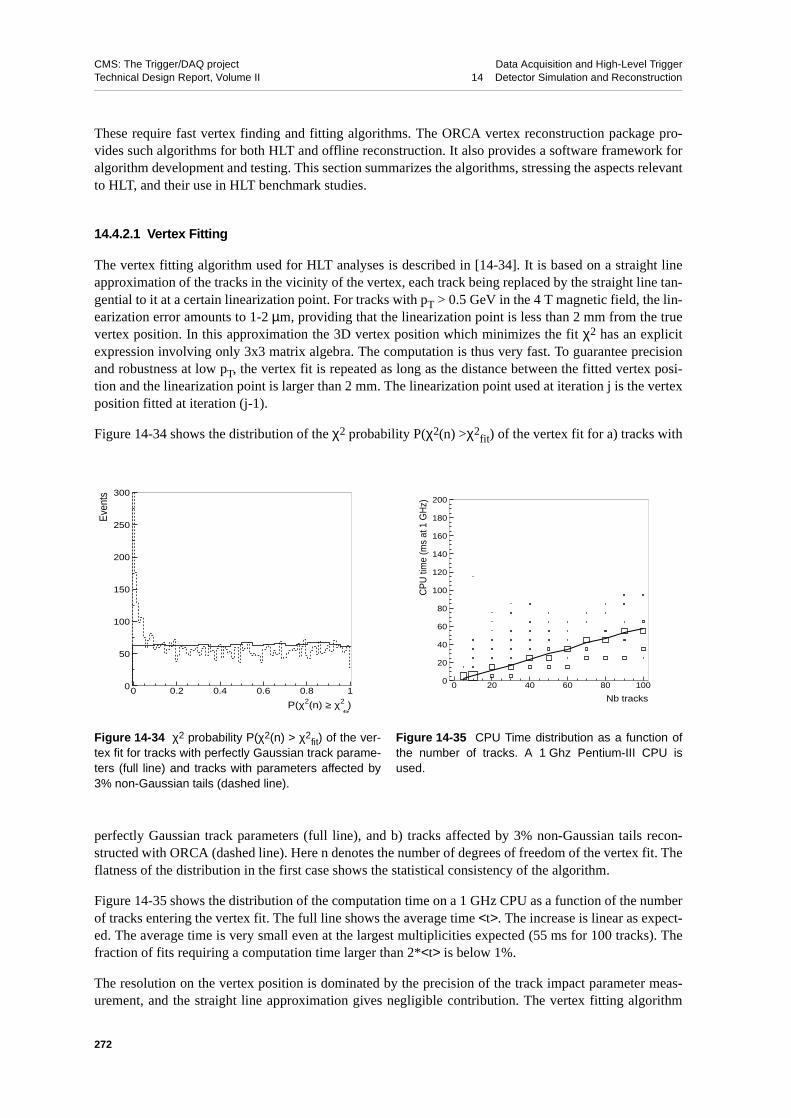
CMS: The Trigger/DAQ project Data Acquisition and High-Level TriggerTechnical Design Report, Volume II 14 Detector Simulation and Reconstruction
These require fast vertex finding and fitting algorithms. The ORCA vertex reconstruction package pro-vides such algorithms for both HLT and offline reconstruction. It also provides a software framework foralgorithm development and testing. This section summarizes the algorithms, stressing the aspects relevantto HLT, and their use in HLT benchmark studies.
14.4.2.1 Vertex Fitting
The vertex fitting algorithm used for HLT analyses is described in [14-34]. It is based on a straight lineapproximation of the tracks in the vicinity of the vertex, each track being replaced by the straight line tan-gential to it at a certain linearization point. For tracks with pT > 0.5 GeV in the 4 T magnetic field, the lin-earization error amounts to 1-2 µm, providing that the linearization point is less than 2 mm from the truevertex position. In this approximation the 3D vertex position which minimizes the fit χ2 has an explicitexpression involving only 3x3 matrix algebra. The computation is thus very fast. To guarantee precisionand robustness at low pT, the vertex fit is repeated as long as the distance between the fitted vertex posi-tion and the linearization point is larger than 2 mm. The linearization point used at iteration j is the vertexposition fitted at iteration (j-1).
Figure 14-34 shows the distribution of the χ2 probability P(χ2(n) >χ2fit) of the vertex fit for a) tracks with
perfectly Gaussian track parameters (full line), and b) tracks affected by 3% non-Gaussian tails recon-structed with ORCA (dashed line). Here n denotes the number of degrees of freedom of the vertex fit. Theflatness of the distribution in the first case shows the statistical consistency of the algorithm.
Figure 14-35 shows the distribution of the computation time on a 1 GHz CPU as a function of the numberof tracks entering the vertex fit. The full line shows the average time <t>. The increase is linear as expect-ed. The average time is very small even at the largest multiplicities expected (55 ms for 100 tracks). Thefraction of fits requiring a computation time larger than 2*<t> is below 1%.
The resolution on the vertex position is dominated by the precision of the track impact parameter meas-urement, and the straight line approximation gives negligible contribution. The vertex fitting algorithm
Figure 14-34 χ2 probability P(χ2(n) > χ2fit) of the ver-
tex fit for tracks with perfectly Gaussian track parame-ters (full line) and tracks with parameters affected by3% non-Gaussian tails (dashed line).
Figure 14-35 CPU Time distribution as a function ofthe number of tracks. A 1 Ghz Pentium-III CPU isused.
0
50
100
150
200
250
300
0 0.2 0.4 0.6 0.8 1
P(χ2(n) ≥ χ2 fit)
Eve
nts
0
20
40
60
80
100
120
140
160
180
200
0 20 40 60 80 100
Nb tracks
CP
U ti
me
(ms
at 1
GH
z)
272

CMS: The Trigger/DAQ project Data Acquisition and High-Level TriggerTechnical Design Report, Volume II 14 Detector Simulation and Reconstruction
provides an accurate estimation of the vertex position uncertainty. This is shown by the distributions ofthe pulls of the vertex coordinates in Figure 14-36, for tracks with perfectly Gaussian parameters (fullline) and for ORCA tracks in 100 GeV u-jets (dashed line).
The flight path value and significance is used in numerous algorithms, for example in τ-tagging, using thelinearized vertex fitter to fit the three-prong tau decay vertex.
14.4.2.2 Vertex Finding
14.4.2.2.1 Definition of Vertex Finding Efficiency and Fake Rate
The efficiency value is very sensitive to the definition of a “reconstructible” vertex, and to the require-ments on the reconstructed vertex quality. In what follows a simulated vertex is considered to be recon-structible if at least 2 of its tracks have been reconstructed. A reconstructible vertex is defined as found ifit is associated to a reconstructed vertex made out of tracks, the majority (>55%) of which originate fromthe correct simulated vertex. The fraction of tracks which originate from the correct simulated vertex iscalled the purity of the reconstructed vertex. This definition of efficiency is adequate for comparing ver-tex finding algorithms, since it is sensitive to small differences in performance. It leads to low efficiencyin b-jets since tracks from the decay chain are mixed. Such merged vertices are still useful for b-tagging,as shown later in the text. The fake rate is defined as the number of reconstructed vertices per event,which have no associated simulated vertex.
14.4.2.2.2 Pixel Primary Vertex Finding
With 3 pixel hits per track one can approximately reconstruct tracks and find primary vertices (PVs) usingthe pixel detector only. At low luminosity, when only two pixel barrel layers are available, the transversebeam constraint can be used. A summary of the algorithms follows.
Pixel hits are matched in r-φ and r-z to establish track candidates. Using these tracks, a list of primary ver-tices is formed with z values where at least three tracks cross the z axis. Tracks which do not point to any
Figure 14-36 Pulls of the vertex coordinates for tracks with perfectly Gaussian parameters (full line) and forORCA tracks in 100 GeV u-jets (dashed line).
273

CMS: The Trigger/DAQ project Data Acquisition and High-Level TriggerTechnical Design Report, Volume II 14 Detector Simulation and Reconstruction
vertex candidate are erased. The algorithm results in a list of primary vertices and lists of tracks attachedto each vertex. The hit matching cuts have been optimized to reconstruct tracks above 1 GeV/c in PT. Forall event types which have been simulated the track finding efficiency is above 90% with the number ofghosts being between 1% and 10%.
The PV candidates found during the track finding stage are re-analyzed. Only PVs with at least 3 validtracks are kept and the position of each vertex is estimated as the mean value of the z impact parametersof all tracks assigned to it. In addition to the main ‘‘signal’’ PV, on the average 6 to 8 more PVs per eventare found at high luminosity. The signal PV is usually found with a high accuracy of better than 50 µm.This is shown in Figure 14-37 where the difference in the z position of the reconstructed vertex and theMonte Carlo vertex is plotted. The efficiency of this algorithm is high; in the HLT event samples the sig-nal PV is always found with an efficiency of better than 95%.
14.4.2.3 Secondary Vertex Finding: Principal Vertex Finder
The recursive secondary vertex finding algorithm finds the principal vertex among a set of tracks: it fitsall tracks to a common vertex, separates the incompatible tracks, stores the cleaned-up vertex if its χ2 issmall enough, and searches for additional vertices in the set of tracks discarded in the previous iteration. Itonly has two parameters to tune: the cut on the probability of compatibility of a track to a vertex, and thecut on the vertex fit χ2. It is thus simple to optimize, and even more so since meaningful cut values areguided by statistics (the default cuts at 5% in probability are optimal in all physics cases tested so far).However since the algorithm has to test the compatibility of each track to the fitted vertex at each itera-tion, the CPU time is expected to rise as N2, where N is the initial number of tracks.
Figure 14-38 shows the efficiency to find a reconstructible secondary vertex inside a b-jet, as a functionof the jet ET and η. The average efficiency is ~30%. The inefficiency is due to the following reasons:
• often there are less than two tracks which are significantly displaced from the primary vertex andwhich can make a secondary vertex. This is visible in Figure 14-39 showing the efficiency versusthe impact parameter significance of the track with the 2nd largest impact parameter. This effect ac-counts for 20% of the inefficiency;
Figure 14-37 The difference (in cm) between the z position of the Monte Carlo primary vertex and the recon-structed primary vertex. Only pixel hits are used in the vertex reconstruction.
0
50
100
150
200
250
300
-0.03 -0.02 -0.01 0 0.01 0.02 0.03Zreconstructed-Zmc(cm)
Cou
nts
274

CMS: The Trigger/DAQ project Data Acquisition and High-Level TriggerTechnical Design Report, Volume II 14 Detector Simulation and Reconstruction
• vertices from the b-decay chain get mixed and lead to reconstructed vertices of low purity. The pu-rity cut accounts for another 20% of inefficiency, as shown in Figure 14-39 when relaxing the puri-ty cut down to 39%.
The fake rate of secondary vertices of this algorithm is very low. In uu events with 100 GeV u-jets, itamounts to five fake vertices per 1000 events.
Figure 14-40 shows the CPU time spent using the principal vertex finder, normalized to a 1 GHz CPU, asa function of the number of tracks on input. The computation time increases as N2 as expected. The CPUtime remains below 20 ms for multiplicities below 10. This multiplicity is characteristic of 100 GeVb-jets, inside a cone of ∆R = 0.4 around the jet axis, containing 95% of the tracks from the b-decay chain.
Figure 14-38 Efficiency to find a reconstructible secondary vertex inside a b-jet, as a function of the jet ET andη, with the Kalman Filter track reconstruction (KF) and with an algorithm providing a better estimation of thetrack parameter errors (Deterministic Annealing Filter, DAF).
Figure 14-39 Secondary vertex efficiency versusimpact parameter significance of the track with the 2nd
largest impact parameter.
Figure 14-40 CPU time for vertex reconstructionusing the principal vertex finder, as a function of thenumber of tracks on input. A 1 GHz Intel Pentium-IIICPU is used.
0
0.05
0.1
0.15
0.2
0.25
0.3
0.35
0.4
0.45
0.5
0 0.25 0.5 0.75 1 1.25 1.5 1.75 2 2.25 2.5
η of b-jet
S.V.
effi
cien
cy
50 GeV
KF
DAF
0
0.05
0.1
0.15
0.2
0.25
0.3
0.35
0.4
0.45
0.5
0 0.25 0.5 0.75 1 1.25 1.5 1.75 2 2.25 2.5
η of b-jet
S.V
. effi
cien
cy
100 GeV
KF
DAF
0
0.1
0.2
0.3
0.4
0.5
0.6
0.7
0.8
0 2 4 6 8 10 12 14 16 18 20
2nd largest d0/σ(d0)
Effi
cien
cy
Purity ≥ 0.55
Purity ≥ 0.39
0
20
40
60
80
100
120
140
160
180
200
0 5 10 15 20 25 30 35 40
Nb tracks
CPU
tim
e (m
s at
1 G
Hz)
275

CMS: The Trigger/DAQ project Data Acquisition and High-Level TriggerTechnical Design Report, Volume II 14 Detector Simulation and Reconstruction
The CPU performance means that even inclusive secondary vertex finding should be affordable at HLT,e.g. for b-tagging purposes.
14.4.3 High-Level Trigger (HLT) Tracking
Track reconstruction for the HLT is special in two respects:
• it is typically guided by external information from a Level-1 Trigger or a High-Level Trigger can-didate. This external input defines one or more regions for track reconstruction;
• it has to address specific questions, such as verifying that the transverse momentum of a Level-2muon candidate is above a threshold, whether a jet is a b-jet or whether an electron is isolated. Inmost cases the answer can be given without fully reconstructing all tracks in the region in question.
These two aspects lead naturally to the concepts of regional, partial and conditional track reconstruction.Most importantly, the CPU time available for a trigger decision must be kept to a minimum. ThereforeHLT track reconstruction concentrates on reducing the number of seeds to a low level, and in minimisingthe number of operations per seed. The first goal is achieved with a regional seed generator whereas thesecond goal is achieved with partial, or conditional, trajectory building.
14.4.3.1 Tracking Region and Regional Seeding
A tracking region is 5-dimensional since a helix is 5-dimensional. These dimensions, and therefore thecorresponding constraints which can be put on the region, are conveniently represented as:
• 2 positions: the transverse and longitudinal impact parameter with respect to the interaction region;
• 2 directions: the pseudorapidity and the azimuthal angle;
• the transverse momentum, PT.
All five constraints can be used to limit the number of seeds. In fact, the standard seed generator alreadyuses the constraints on the size of the origin and on the minimal transverse momentum(Section 14.4.1.2.1). In addition, the regional seed generator uses the angular constraints to restrict thehits on the seeding layers. The resulting seeds are compatible with the tracking region.
For each seeding layer a measurement estimator matching the size of the tracking region is constructed,and the hits from the layer are requested using this estimator. The DetLayer uses the estimator first to findthe compatible detectors, and then to filter the hits from the compatible detectors. The detectors which arenot compatible with the tracking region are never accessed for hits, and their digis (raw data) are never ac-cessed. Since the loading of the detector raw data happens on demand, this automatically ensures thatonly the minimal necessary amount of raw data will be accessed and clustered.
The reduction factor in number of seeds depends on the size of the region, which in turn depends on thephysics. In some cases, like trigger muon reconstruction, the constraints on transverse impact parameter,momentum, and angles are sufficiently strong to reduce the number of seeds below 100, even without anyknowledge of the z position of the primary vertex of the signal event. In other cases, like b-tagging of ajet, the number of seeds in the jet cone is too big for direct reconstruction (of the order of 2000 at high lu-minosity for a cone size of interest). In such cases knowledge of the z position of the signal primary ver-tex is required to reduce further the number of seeds.
The pixel vertex reconstruction, described in Section 14.4.2.2.2, provides primary vertex candidates with-out prior track reconstruction, and within the CPU time available at HLT, up to the full Level-1 rate. The
276

CMS: The Trigger/DAQ project Data Acquisition and High-Level TriggerTechnical Design Report, Volume II 14 Detector Simulation and Reconstruction
elimination of all seeds not compatible with primary vertex candidates results in an acceptable number ofseeds within an acceptable CPU time.
14.4.3.2 Partial (Conditional) Track Reconstruction
The trajectory-building stage is affected significantly by the momentum constraint which provides a use-ful speed-up since trajectory candidates with PT below the cut are abandoned immediately. The other con-straints are not very helpful: if the seed is within the tracking region, the resulting track is very likely to beinside thne regionas well. The speed of trajectory building can be increased, at the cost of reconstructionefficiency, by tuning the various parameters that control the number of combinations and the acceptablenumber of inefficient layers. However, for algorithmic efficiencies above 97% the savings in CPU are notsubstantial.
The idea of partial reconstruction goes beyond the tuning of algorithmic parameters. Starting from a HLTobject specification it addresses the minimum reconstruction needed to provide the information neededby the requirement. A simple example helps illustrate the process: if an electron or a muon is already re-constructed and passes the trigger criteria, and the next step is to check if it is isolated, the following stepsmust be performed:
• the seeds in the isolation cone must be constructed. The z impact parameter of the trigger leptoncan be used to define the signal vertex and thus reduce the number of seeds;
• trajectory-building must proceed for all seeds until enough tracks are reconstructed to fail the isola-tion criteria. Typically, as soon as one or two tracks are found, the lepton can be classified asnon-isolated, rendering the reconstruction of any remaining seeds unnecessary.
If the rejection factor of this trigger is high, i.e. most leptons are not isolated, and if the average multiplic-ity in the isolation cone is high, the gain in CPU time can be substantial.
Conditional reconstruction works particularly well in restricting the trajectory-building process. Recon-structed tracks are used only if they satisfy some selection criteria. If it is possible to recognise at an earlystage of trajectory building, that a track candidate fails the selection, then the reconstruction of this candi-date can be stopped, and the CPU time saved. Again, an example can illustrate this.
Almost every set of physics-object selection criteria has a requirement on the minimum PT of the object.The PT is in turn known after each update step in the Kalman filter. For a real track, adding subsequenthits cannot modify the momentum significantly at any point along the track. Using a Guassian approxi-mation, the change in track parameters should be smaller than a number of standard deviations on the mo-mentum measurement. It is therefore safe to stop the reconstruction of any trajectory candidate if itscurrent PT drops e.g. 5 σ below the cut value, even if there are only three hits on the track. This is called astopping condition for trajectory building.
As for the seed generator, the minimal PT condition is always present in the trajectory builder since thereis always a value below which reconstruction is not sensible. This reduces significantly the CPU time(this is the only use of the Tracking Region in the trajectory builder).
This is the essence of conditional trajectory building: tracks are reconstructed until some condition is met.A generic interface allows the specification of an unlimited number of stopping conditions. Some condi-tions are expensive to verify numerically. For example, for b-tagging it is important to reconstruct a trackuntil the accuracy of the impact parameter is sufficient, or the impact parameter is significant. However,in an “inside-out” Kalman filter (as is the case with pixel seeds) the track parameters are not known at theinteraction point until the smoothing stage. It would be too expensive computationally to smooth each
277

CMS: The Trigger/DAQ project Data Acquisition and High-Level TriggerTechnical Design Report, Volume II 14 Detector Simulation and Reconstruction
candidate after each update with a new hit, only to check if the precision or significance on the impact pa-rameter is reached.
A study of the accuracy on track parameters as a function of the number of hits in the track, shown inFigure 14-41, reveals that asymptotic accuracy on the impact parameter is reached after only 5 or 6 hits.This is true for a large range in momentum and in pseudorapidity, covering the physically interesting re-gion. Therefore, the most commonly used stopping condition for HLT tracking is to limit the number ofhits in a track to 5 or 6, provided the ghost track rate is acceptable. Figure 14-42 also shows the error onthe track 2D impact parameter as a function of the number of hits along the track. Using tracks with 5 hitsthe precision is comparable to the full reconstruction. A reduced number of hits along the track, however,increases the fraction of ghost tracks.
Figure 14-42 compares the efficiency for track reconstruction with the fraction of ghost tracks as a func-tion of the number of hits along the track, for different η ranges. The efficiency for track reconstructiondecreases slightly with increasing the number of hits, mainly due to nuclear interactions in the detector.The fake rate decreases to below the 1% for tracks with at least six hits. In the case of staged pixel detec-tor the fake rate increases considerably for the same number of hits.
14.5 References
14-1 V. Innocente, L. Silvestris and D. Stickland, on behalf of the CMS collaboration, “CMS Software Architecture. Software framework, services and persistency in High-Level trigger, reconstruction and analysis”, Comput. Phys. Commun., 140 (2001) 31; Coherent Object Base for Reconstruction, Analysis and simulation (COBRA), see http://cobra.web.cern.ch/cobra/.
14-2 T. Sjostrand et al., “High Energy Physics Event Generation with PYTHIA 6.1”, hep-ph/0010017, LU TP 00-30; also S. Mrenna, “SPYTHIA, A Supersymmetric Extension of PYTHIA 5.7”, Comput. Phys. Commun. 101 (1997) 232.
Figure 14-41 The resolution on a) PT and b) impact parameter for partial track reconstruction, compared withfull track reconstruction, as a function of the number of smoothing steps in different PT and for the barrelregion.The leftmost point at “0” reconstructed hits shows the full tracker performance.
(a)
Reconstructed Hits
σ(p tre
c -p tsi
m)[
GeV
/c]
0.05
0.1
0.15
0.2
0.25
0 2 4 6 8 10 12
(b)
Reconstructed Hits
σ(d 0re
c -d 0si
m)[µ
m]
20
30
40
50
60
70
80
0 2 4 6 8 10 12
278

CMS: The Trigger/DAQ project Data Acquisition and High-Level TriggerTechnical Design Report, Volume II 14 Detector Simulation and Reconstruction
14-3 F. Paige and S. Protopopescu, in Supercollider Physics, p.41, ed. D. Soper (World Scientific, 1986); also H. Baer et al., in Proceedings of the Workshop on Physics at Current Accelerators and Supercolliders, ed. J. Hewett, A. White and D. Zeppenfeld, (Argonne National Laboratory, 1993).
14-4 N. Amapane et al., “Monte Carlo Simulation of Inclusive Single- and Di-Muon Samples”, CMS Note 2002/041.
14-5 H. Sakulin, “Methodology for the Simulation of Single-Muon and Di-Muon Trigger Rates at the CMS Experiment in the Presence of Pile–Up”, CMS Note 2002/042.
14-6 D. Acosta, M. Stoutimore, and S.M. Wang, “Simulated Performance of the CSC Track-Finder”, CMS Note 2001/033.
14-7 M. Huhtinen, “Optimization of the CMS Forward Shielding”, CMS Note 2000/068.
14-8 G. Bruno and M. Konecki, “Simulation of the Baseline RPC Trigger System for CMS: Efficiency and Output Rates in Single Muon Topology “, CMS Note 2001/012.
14-9 CMS Simulation Package CMSIM — Users' Guide and Reference Manual, http://cmsdoc.cern.ch/cmsim/cmsim.html
14-10 GEANT3, version 3.21/13 (release 15111999), Detector Description and Simulation Tool, CERN program library long writeup W5013.
14-11 CMS Coll.,“The Electromagnetic Calorimeter Project, Technical Design Report”, CERN/LHCC 97-33, CMS TDR 4, 15 December 1997.
14-12 1999 Status Report on the RD-12 Project, CERN/LHCC 2000-002, 3 January 2000.
14-13 V. V. Abramov et al., "Studies of the response of the prototype CMS hadron calorimeter, including magnetic field effects, to pion, electron, and muon beams", Nucl. Instr. and Meth. A 457 (2001) 75.
14-14 D. Litvintsev, “Detailed Monte Carlo program for Quartz Very Forward Calorimeter for CMS Detector”, CMS Technical Note 1995/098.
14-15 GLANDZ, see http://wwwinfo.cern.ch/asdoc/geantold/GEANTMAIN.html
14-16 RAL Micro-electronics Design Group, “APV25 User Guide”, http://www.te.rl.ac.uk/med/projects/High_Energy_Physics/CMS/APV25-S1/pdf/User_Guide_2.0.pdf
Figure 14-42 Efficiency (left axis) and ghost rate (right axis) for track reconstruction as a function of the numberof hits along the track for 100 GeV jets. The left plot is for b tracks and the right plot for u-jet tracks.
No. of hits
Effic
iency
No. of hitsF
ake
Rate
bb − jets ET=100 GeV L=2x1033 cm-2s-1
Efficiency 0.<|η|<1.4Efficiency 1.4<|η|<2.4Fake Rate 0.<|η|<1.4Fake Rate 1.4<|η|<2.4
(a)
0
0.1
0.2
0.3
0.4
0.5
0.6
0.7
0.8
0.9
1
4 5 6 7 8 9 100
0.1
0.2
0.3
0.4
0.5
0.6
4 5 6 7 8 9 10
No. of hits
Effic
iency
No. of hits
Fake
Rate
uu − jets ET=100 GeV L=2x1033 cm-2s-1
Efficiency 0.<|η|<1.4Efficiency 1.4<|η|<2.4Fake Rate 0.<|η|<1.4Fake Rate 1.4<|η|<2.4
(b)
0
0.1
0.2
0.3
0.4
0.5
0.6
0.7
0.8
0.9
1
4 5 6 7 8 9 100
0.1
0.2
0.3
0.4
0.5
0.6
4 5 6 7 8 9 10
279

CMS: The Trigger/DAQ project Data Acquisition and High-Level TriggerTechnical Design Report, Volume II 14 Detector Simulation and Reconstruction
14-17 M. Raymond et al., “ The CMS Tracker APV25 0.25um CMOS Readout Chip”, in Proceedings of the 6th Workshop on Electronics for LHC Experiments, Cracow, Poland, 11-15 September 2000, pp. 130-134.
14-18 R.Veenhof, CERN program library long writeup W5050, GARFIELD.
14-19 A. Gresele and T.Rovelli, “Parametrization of B Field Effects in DTBx”, CMS Note 1999/064.
14-20 CMS Coll.,“The Muon Project, Technical Design Report”, CERN/LHCC 97-32, CMS TDR 3, 15 December 1997.
14-21 M.Aguilar-Benitez at al., “Construction and Test of the final CMS Barrel Drift Tube Muon Chamber Prototype”, Nucl. Instr. and Meth. A480 (2002) 658; M. Cerrada et al., “Results from the Analysis of the Test Beam Data taken with the Barrel Muon DT Prototype Q4”, CMS Note 2001/041.
14-22 R. Wilkinson and P.T. Cox, “Simulating the Endcap Muon CSC System in ORCA”, CMS Note 2001/013.
14-23 E. Gatti et al., “Analysis of the position resolution in centroid measurements in MWPC”, Nucl. Instr. and Meth. 188 (1981) 327.
14-24 K.W. Bell et al., “User Requirements Document for the Final FED of the CMS Silicon Strip Tracker”, CMS Note 2001/043.
14-25 O. Kodolova, I. Tomalin and P. Yepes, “Expected Data Rates from the Silicon Strip Tracker”, CMS Note-2002/047.
14-26 B. Baur et al. ,”Heavy Ion Physics Programme in CMS”, CMS Note 2000/060.
14-27 .CMS Coll.,“The Magnet Project, Technical Design Report”, CERN/LHCC 97-10, CMS TDR 1, 2 May 1997.
14-28 S. Cucciarelli, D. Kotlinski and T. Todorov, “Position Determination of Pixel Hits”, CMS Note 2002/049.
14-29 M. Winkler, PhD Thesis, 2002/015.
14-30 R. Fruhwirth, Nucl. Instr. and Meth. A262 (1987) 444.
14-31 K.Hagiwara et al., Phys.Rev. D66 (2002) 010001, and references therein.
14-32 H.A. Bethe and W .Heitler, Proc.R.Soc.London A146 (1934) 83.
14-33 V. Innocente, M. Maire, and E. Nagy, CERN program library long writeup W5013-E, GEANE.
14-34 V. Karimaki, “Effective vertex fitting”, CMS Note 1997/051.
14-35 CMS Coll.,“The Trigger and Data Acquisition project, Volume I, The Level-1 Trigger, Technical Design Report”, CERN/LHCC 2000-038, CMS TDR 6.1, 15 December 2000.
280

CMS: The Trigger/DAQ project Data Acquisition and High-Level TriggerTechnical Design Report, Volume II 15 Physics Object Selection and HLT Performance
15 Physics Object Selection and HLT Performance
This chapter discusses the reconstruction and selection of physics objects in the High-Level Trigger.These objects constitute candidates for electrons, muons, neutrinos (as missing energy), and hadronic jets,as well as jets tagged as originating from tau leptons or b-quarks. For each object, the efficiency and puri-ty of the reconstruction and selection are estimated. In the end, a “trigger table”, i.e. a set of kinematic re-quirements on each object, leading to an output rate to storage consistent with the current capability ofO(102) Hz, is produced.
The chapter is organized as follows: an overview of the physics requirements and the general guidelinesused in the development of the HLT algorithms can be found in Section 15.1. The following sections de-scribe the reconstruction algorithms, the selection and the CPU requirements for the identification of eachphysics object. Section 15.7 describes the samples and procedures needed for the calibration of the CMSsubdetectors, as well as for the monitoring of the performance of the HLT. The chapter concludes with asummary of all thresholds for selecting physics objects for storage, the overall CPU requirements of theHLT and the efficiency for some key physics channels in Section 15.8.
15.1 Overview of Physics Reconstruction and Selection
The key aspect of the High-Level Trigger which runs in the Filter Farm is the real-time nature of the se-lection. This imposes significant constraints on the resources that the algorithms can use and on the relia-bility of these algorithms. Events rejected by the HLT, with the exception of very small samples retainedfor monitoring of the HLT performance, are lost forever. The correct functioning of the HLT is therefore akey issue for the CMS physics program.
The next section discusses the physics requirements of the online selection while the strategy used in im-plementing the software is described next. The allocation of bandwidth to different physics objects atLevel-1 is the subject of the last section.
15.1.1 Physics Requirements
The main requirements from the physics point of view are:
• foremost, the requirement that the selection fulfill the needs of the CMS physics program; the effi-ciency for the physics objects must be as high as possible;
• the selection must be as inclusive as possible. The LHC represents a new energy frontier, and un-expected new phenomena may appear. The selection requirements must not reject events of poten-tial use in such exotic searches;
• all thresholds and other requirements applied by the selection should be such that detailed knowl-edge of calibration constants and other run conditions is not necessary in real-time;
• the final selection of events should include data samples for the calculation of all trigger and recon-struction efficiencies offline;
• the rate of events accepted by the HLT should be within limits, i.e. approximately O(102) Hz;
• all algorithms and code should be monitored continually for their correct functioning;
• the events selected by the HLT should be tagged to indicate the reasons for their selection, to aidthe offline reconstruction;
281

CMS: The Trigger/DAQ project Data Acquisition and High-Level TriggerTechnical Design Report, Volume II 15 Physics Object Selection and HLT Performance
• the HLT should include all major improvements in the offline reconstruction, and thus it should beas close as possible to the standard offline reconstruction code.
Above all, the HLT selection must be reliable and robust. Every event that will be used by CMS for thevery rich physics program it expects to carry out must be accepted by the High-Level Trigger. The HLT isthus a crucial element for the success of the CMS experimental program.
15.1.2 Selection Strategy and Reconstruction on Demand
As discussed in Chapter 1, "Overview", the CMS DAQ/HLT complex processes all events accepted bythe Level-1 Trigger in a single processor farm. There is therefore no “Level-2” or “Level-3” trigger inCMS, but a single entity, the “High-Level Trigger”, or HLT. Nevertheless, as in a traditional multi-levelsystem, the selection of events can be optimized by rejecting events as quickly as possible. For this reasonthe basic reconstruction strategy is to reconstruct those parts of each physics object that can be used forselection while minimizing the overall CPU usage.
As an example, as described in Section 15.2, "Electron/Photon Identification", reconstruction of an elec-tron includes the reconstruction of a cluster in the electromagnetic calorimeter, the matching of hits in thepixel detector and the subsequent reconstruction of a full charged particle track in the tracker. At the endof each step a set of selection criteria results in the rejection of a significant fraction of the events accept-ed by the previous step. The rate of events that need to be processed through the remaining algorithms isdecreased thus reducing the required CPU. Reconstruction and selection are therefore closely intertwinedin the online environment of the filter farm. For an optimal system the HLT should reconstruct the mini-mum amount of detector information needed to apply a set of selection criteria that reject backgroundevents while keeping the desired physics events for further processing.
15.1.2.1 Trigger Levels — Definitions
The reconstruction and selection in the HLT takes place in steps which correspond roughly to what wouldhave been distinct trigger systems, the Level-2 and Level-3 trigger systems. It is thus convenient to usethe terminology, and to refer to a “Level-2 trigger” or a “Level-3 step” to describe the selection algo-rithms and criteria of the HLT. Clearly, in the case of the CMS HLT there is no sharp division betweenthese trigger steps, other than the order in which they are applied.
In what follows, the convention used is that “Level-2” triggers, algorithms and requirements refer to thefirst selection step in the HLT process. Typically, a Level-2 trigger, which has the maximum rate of eventsinput to it, uses information from only the calorimeter and muon detectors. In contrast, “Level-3” refers toselection that includes the reconstruction of full tracks in the tracker. Traditionally, because of the highnumber of channels, the complex pattern recognition and higher combinatorics, track reconstruction is aprocess that demands large amounts of CPU time. Carrying the analogy even further, in what followsthere are references to “Level-2.5” triggers, which refer to algorithms that use partial tracker information,e.g. pixel hits for a fast confirmation of the electron candidate. The numbering, “2.5”, attempts to indicatethe intermediate nature of the selection, as one that occurs between the selection that is based solely onthe calorimeter information, and the selection that is based on the full CMS detector information.
As described in the previous chapter, reconstruction of charged particle tracks in the CMS detector hasturned out to be a task that demands less CPU time than is normally expected, and for this reason some ofthe selection algorithms may change in the future. As an example, if full charged-track reconstructionever becomes faster than the fast pixel reconstruction in the electron selection, the two steps will be inter-changed in the HLT. This flexibility is the major advantage of executing the full selection in a single proc-
282

CMS: The Trigger/DAQ project Data Acquisition and High-Level TriggerTechnical Design Report, Volume II 15 Physics Object Selection and HLT Performance
essor farm: the system can make optimal use of the most recent advances not only in computing but alsoin the algorithms and software developed in the experiment.
15.1.2.2 Partial Event Reconstruction
To minimize the CPU required by the HLT, a key feature of the algorithms is to reconstruct the informa-tion in the CMS detector only partially. In many cases the decision on whether an event should be accept-ed by the HLT involves the reconstruction of quantities in only a limited region of the detector. As anexample, for an event accepted by the Level-1 Trigger in the inclusive muon stream, only the parts of themuon chambers pointed to by the Level-1 Trigger information, and the corresponding road in the tracker,need be considered for the validation of the muon.
The idea of partial event reconstruction has been embedded in the CMS reconstruction code from the verybeginning. In the case of the HLT, the reconstruction of physics objects is driven by the correspondingcandidates identified by the Level-1 Trigger. Except in a few cases, which are indicated, all reconstructiondescribed in this chapter starts from the Level-1 Trigger information. This approach leads to significantCPU savings, however it also leads to rejecting events that contain “volunteer” objects, i.e. objects thatdid not pass the Level-1 Trigger. This disadvantage is mitigated by the fact that it is, in general, very dif-ficult to understand the properties of such objects in later offline analyses. It is clearly always feasible, al-beit with an increased CPU cost, to look for additional objects in each event if a particular physicsanalysis raises such a requirement.
15.1.3 Level-1 Trigger Settings and Rates
The performance of the Level-1 Trigger system is summarized in Appendix F, "Summary of Level-1Trigger" while the full details of the system can be found in the Trigger TDR [15-1]. There have beensome minor changes in rates and efficiencies with respect to that document. The changes reflect the newMonte Carlo input, including an updated version of the PYTHIA Monte Carlo (to version 6) and much in-creased statistics in the Monte Carlo samples generated, as well as a more detailed and tuned detectorsimulation. The main thrust of the conclusions of reference [15-1] remains unchanged: the overall per-formance of the system satisfies the requirements of the CMS physics program.
Another change with respect to the Trigger TDR is the definition of the low luminosity run conditions:“low” luminosity in this document refers to an instantaneous luminosity of 2×1033 cm-2s-1, while “high”luminosity refers to the nominal LHC design value of 1034 cm-2s-1. As discussed in Chapter 17, the cur-rent plans of CMS call for a phased installation of the Data Acquisition system so that at start-up the DAQcan handle an event rate of up to 50 kHz and at the full design luminosity it can handle a rate of 100 kHz.
The allocation of the Level-1 Trigger bandwidth must be optimized in order to ensure the widest possiblephysics reach for the experiment, while including all technical triggers intended for calibration and moni-toring of the detector. The procedure used for this optimization starts with a determination of the maxi-mum Level-1 Trigger rate that can be allocated, which is 16 kHz at low luminosity and 33 kHz at highluminosity. These maximum rates arise from dividing total DAQ bandwidth, i.e. 50 kHz (100kHz) at low(high) luminosity, by a safety factor of three. This safety factor is used to account for all uncertainties inthe simulation of the basic physics processes, the CMS detector, and the beam conditions.
The second step is a first allocation of this Level-1 bandwidth across the different objects. An equal allo-cation across the four categories of “objects”, taken as (a) electrons/photons, (b) muons, (c) tau-jets and(d) jets plus combined channels, is made. For example, at low luminosity 4 kHz is pre-allocated to each ofthese triggers.
283
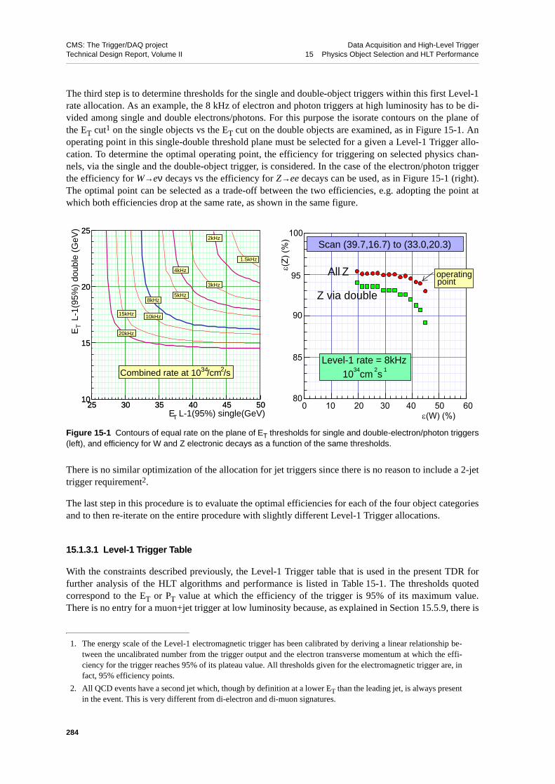
CMS: The Trigger/DAQ project Data Acquisition and High-Level TriggerTechnical Design Report, Volume II 15 Physics Object Selection and HLT Performance
The third step is to determine thresholds for the single and double-object triggers within this first Level-1rate allocation. As an example, the 8 kHz of electron and photon triggers at high luminosity has to be di-vided among single and double electrons/photons. For this purpose the isorate contours on the plane ofthe ET cut1 on the single objects vs the ET cut on the double objects are examined, as in Figure 15-1. Anoperating point in this single-double threshold plane must be selected for a given a Level-1 Trigger allo-cation. To determine the optimal operating point, the efficiency for triggering on selected physics chan-nels, via the single and the double-object trigger, is considered. In the case of the electron/photon triggerthe efficiency for W→eν decays vs the efficiency for Z→ee decays can be used, as in Figure 15-1 (right).The optimal point can be selected as a trade-off between the two efficiencies, e.g. adopting the point atwhich both efficiencies drop at the same rate, as shown in the same figure.
There is no similar optimization of the allocation for jet triggers since there is no reason to include a 2-jettrigger requirement2.
The last step in this procedure is to evaluate the optimal efficiencies for each of the four object categoriesand to then re-iterate on the entire procedure with slightly different Level-1 Trigger allocations.
15.1.3.1 Level-1 Trigger Table
With the constraints described previously, the Level-1 Trigger table that is used in the present TDR forfurther analysis of the HLT algorithms and performance is listed in Table 15-1. The thresholds quotedcorrespond to the ET or PT value at which the efficiency of the trigger is 95% of its maximum value.There is no entry for a muon+jet trigger at low luminosity because, as explained in Section 15.5.9, there is
1. The energy scale of the Level-1 electromagnetic trigger has been calibrated by deriving a linear relationship be-tween the uncalibrated number from the trigger output and the electron transverse momentum at which the effi-ciency for the trigger reaches 95% of its plateau value. All thresholds given for the electromagnetic trigger are, infact, 95% efficiency points.
Figure 15-1 Contours of equal rate on the plane of ET thresholds for single and double-electron/photon triggers(left), and efficiency for W and Z electronic decays as a function of the same thresholds.
2. All QCD events have a second jet which, though by definition at a lower ET than the leading jet, is always presentin the event. This is very different from di-electron and di-muon signatures.
10
15
20
25
25 30 35 40 45 5010
15
20
25
25 30 35 40 45 50ET L-1(95%) single(GeV)
ET L
-1(9
5%)
doub
le (
GeV
)
1.5kHz
2kHz
3kHz
4kHz
5kHz 8kHz
10kHz15kHz
20kHz
Combined rate at 1034/cm2 /s
80
85
90
95
100
0 10 20 30 40 50 60ε(W) (%)
operatingpoint
All Z
Z via double
Scan (39.7,16.7) to (33.0,20.3)
1034
cm2s
1Level-1 rate = 8kHz
ε(Z)
(%)
284
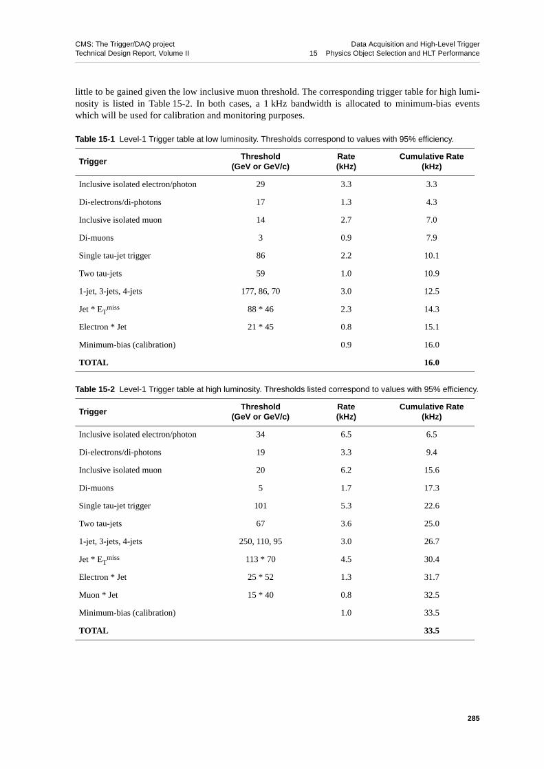
CMS: The Trigger/DAQ project Data Acquisition and High-Level TriggerTechnical Design Report, Volume II 15 Physics Object Selection and HLT Performance
little to be gained given the low inclusive muon threshold. The corresponding trigger table for high lumi-nosity is listed in Table 15-2. In both cases, a 1 kHz bandwidth is allocated to minimum-bias eventswhich will be used for calibration and monitoring purposes.
Table 15-1 Level-1 Trigger table at low luminosity. Thresholds correspond to values with 95% efficiency.
TriggerThreshold
(GeV or GeV/c)Rate (kHz)
Cumulative Rate (kHz)
Inclusive isolated electron/photon 29 3.3 3.3
Di-electrons/di-photons 17 1.3 4.3
Inclusive isolated muon 14 2.7 7.0
Di-muons 3 0.9 7.9
Single tau-jet trigger 86 2.2 10.1
Two tau-jets 59 1.0 10.9
1-jet, 3-jets, 4-jets 177, 86, 70 3.0 12.5
Jet * ETmiss 88 * 46 2.3 14.3
Electron * Jet 21 * 45 0.8 15.1
Minimum-bias (calibration) 0.9 16.0
TOTAL 16.0
Table 15-2 Level-1 Trigger table at high luminosity. Thresholds listed correspond to values with 95% efficiency.
TriggerThreshold
(GeV or GeV/c)Rate (kHz)
Cumulative Rate (kHz)
Inclusive isolated electron/photon 34 6.5 6.5
Di-electrons/di-photons 19 3.3 9.4
Inclusive isolated muon 20 6.2 15.6
Di-muons 5 1.7 17.3
Single tau-jet trigger 101 5.3 22.6
Two tau-jets 67 3.6 25.0
1-jet, 3-jets, 4-jets 250, 110, 95 3.0 26.7
Jet * ETmiss 113 * 70 4.5 30.4
Electron * Jet 25 * 52 1.3 31.7
Muon * Jet 15 * 40 0.8 32.5
Minimum-bias (calibration) 1.0 33.5
TOTAL 33.5
285

CMS: The Trigger/DAQ project Data Acquisition and High-Level TriggerTechnical Design Report, Volume II 15 Physics Object Selection and HLT Performance
15.2 Electron/Photon Identification
The selection of electrons and photons proceeds in three steps. The first step, “Level-2.0”, uses the Calo-rimeter information alone. The next step, “Level-2.5”, demands hits in the pixel detectors consistent withan electron candidate. This matching of an ECAL super-cluster (defined in paragraph 15.2.1) to hits in thepixel detector divides the electromagnetic triggers into two streams: electron candidates (single and dou-ble), and, above significantly higher thresholds, photon candidates. In the final step, “Level-3”, the selec-tion of electrons uses full track reconstruction, seeded from the pixel hits obtained by the matching step.The selection of photons can use isolation cuts and rejection of π0s based on lateral shower shape and thereconstruction of converted photons.
For the calorimeter reconstruction — clustering as well as energy and position measurement — the em-phasis is predominantly on the reconstruction of electrons, rather than photons, because the target trans-verse momentum cuts and thresholds for triggering on electrons are much lower than those for photons.The first challenge for ECAL clustering is to include all energy radiated by electrons in the tracker mate-rial. Photons, including those that have converted in the tracker material, are adequately reconstructed bythe electron algorithms for threshold cuts to be applied. For the final reconstruction of photons with highprecision it is envisaged that unconverted photons will be reconstructed using energy sums of fixed arraysof crystals (probably 5×5 crystals), and that tracker information will be used to assist in the clustering forconverted photons. These algorithms to refine photon energy resolution are not needed for the HLT selec-tion, and have not yet been fully developed, although much of the necessary work has been started instudies of π0 rejection.
15.2.1 Calorimeter Reconstruction: Clustering
The first step in the reconstruction of an electron in the High-Level Trigger is the clustering of the energydeposits in the electromagnetic calorimeter (ECAL) and the estimation of the electron’s energy and posi-tion from this information. In the barrel section this involves the energy deposited in the lead tungstatecrystals alone, in the endcap energy is also deposited in the ~3X0 thick preshower detector.
Electrons radiate in the material between the interaction point and the ECAL. The bending of the electronin the 4T magnetic field results in a spray of energy reaching the ECAL. The spreading of this spray is, togood approximation, only in the ϕ-direction. The electron energy can be collected by making a cluster ofclusters along a ϕ road. This cluster of clusters is called a “super-cluster”.
15.2.1.1 The Island Algorithm
The island algorithm starts by a search for seeds which are defined as crystals with an energy above a cer-tain threshold. Starting from the seed position, adjacent crystals are examined, scanning first in ϕ and thenin η. Along each scan line crystals are added to the cluster until a rise in energy or crystal that has notbeen read out is encountered.
In much the same way as energy is clustered at the level of calorimeter cells, non-overlapping clusters canin turn be clustered into calorimetric “super-clusters”. The procedure is seeded by searching for the mostenergetic cluster and then collecting all the other nearby clusters in a very narrow η-window, and muchwider ϕ-window.
286

CMS: The Trigger/DAQ project Data Acquisition and High-Level TriggerTechnical Design Report, Volume II 15 Physics Object Selection and HLT Performance
15.2.1.2 The Hybrid Algorithm
For single showers, such as those produced by unconverted photons, or those produced by electrons intest beam conditions, energy sums of fixed arrays of crystals give better energy resolution performancethan energy sums of crystals collected dynamically according to a cluster or “bump” finding algorithm.The Hybrid algorithm uses the η−ϕ geometry of the barrel crystals to exploit the knowledge of the lateralshower shape in the η direction (taking a fixed bar of three or five crystals in η), while searching dynam-ically for separated (bremsstrahlung) energy in the ϕ direction.
The Hybrid algorithm is designed to reconstruct relatively high energy electrons in the barrel (so far wehave used it for electrons with PT>10 GeV/c). By contrast, when looking for small deposits of energy inindividual clusters, for example when making a calorimetric isolation cut, the basic clusters of the Islandalgorithm are more appropriate objects to work with. Further details about the clustering algorithms canbe found in reference [15-2].
15.2.2 Endcap Reconstruction with the Preshower
Much of the endcap is covered by a preshower device with two planes of silicon strip readout. The energydeposited in the preshower detector (which is about 3X0 thick) needs to be added to the crystal clusters.The constants relating the energy deposited in the two planes of silicon to the crystal energy are explainedin reference [15-3].
The energy in the crystals is clustered using the Island algorithm and the clusters are associated to formsuper-clusters. A preshower cluster is constructed in each plane, in front of each crystal cluster of the su-per-cluster. The search area in the preshower is centred on the point determined by extrapolating the crys-tal cluster position to the preshower plane in the direction of the nominal vertex position.
15.2.3 Energy and Position Measurement
15.2.3.1 Position Measurement Using Log-weighting Technique
A simple position measurement of the shower can be obtained by calculating the energy-weighted meanposition of the crystals in the cluster. To obtain a precise position measurement two issues need to be con-sidered in more detail.
Firstly, the meaning of crystal position needs to be defined. The crystals in the CMS ECAL are quasi-pro-jective, and do not exactly point to the nominal interaction vertex. So the lateral position (η,ϕ) of the crys-tal axis depends on depth as illustrated in Figure 15-2. A depth tmax thus needs to be defined. This depthis something like the longitudinal centre of gravity of the shower, and its optimal mean value varies loga-rithmically with the shower energy. There is also a dependence on particle type — electron showers havea maximum about one radiation length less deep than photon showers. In the position measurement usedfor both Island and Hybrid super-clusters the depth is measured from the front face of the crystals alongthe direction from the nominal vertex position to the approximate shower position calculated using thearithmetic energy weighted mean of the shower front face centres.
To account for the energy dependence a parametrization is used: A(B + log(E)). The determination of theparameters is described in reference [15-2].
287

CMS: The Trigger/DAQ project Data Acquisition and High-Level TriggerTechnical Design Report, Volume II 15 Physics Object Selection and HLT Performance
The second issue that requires more detailed treatment is related to the lateral shower shape. Since the en-ergy density does not fall away linearly with distance from the shower axis, but rather exponentially, asimple energy weighted mean of crystal energies is distorted and the measured position is biased towardsthe centre of the crystal containing the largest energy deposit.
In earlier studies this bias was removed by applying a position correction (the “S-shape correction” de-scribed in reference [15-4]). A simpler algorithm which yields almost as good precision is used here. Theweighted mean is calculated using the logarithm of the crystal energy:
where xi is the position of crystal i, and Wi is the log weight of the crystal — the log of the fraction of thecluster energy contained in the crystal, calculated with the formula:
where the weight is constrained to be positive, or is otherwise set to zero. W0 then controls the smallestfractional energy that a crystal can have and still contribute to the position measurement. More details canbe found in reference [15-2].
So far what has been described refers to measurement of the position of a single cluster. The position of asuper-cluster is calculated by making the energy-weighted mean of the positions of its component clus-ters. An important point at issue here is that the energy-weighted mean impact position of an electron andthe photons it has radiated in its passage through the tracker material corresponds to the position a non-ra-diating electron would have impacted. It is this position which we wish to measure to enable the correctreconstruction of the original electron from the vertex. So, although it is unimportant for the energy meas-urement whether the crystal energy deposits from the electron and its radiated photons are all collectedinto a single cluster or into separate clusters, correctly clustering the energy deposits improves the ϕmeasurement of an electron. If the electron and a bremsstrahlung photon fall into the same cluster then theweighting of their contributions used is the log weighting appropriate to lateral shower spread, and not thelinear weighting appropriate between the electron and a photon it radiated.
Figure 15-2 Illustration of crystal off-pointing.
crystal axis
nominal pos @ front face
corrected position
tmax
xxi Wi•∑
Wi∑----------------------=
Wi W0
Ei
Ej∑----------
log+=
288

CMS: The Trigger/DAQ project Data Acquisition and High-Level TriggerTechnical Design Report, Volume II 15 Physics Object Selection and HLT Performance
15.2.3.2 Energy Measurement and Corrections
The measurement of energy in the crystals is obtained by simple addition of the deposits measured in thecrystals — although more complex estimators have been envisaged [15-5].
Even in the areas not covered by the preshower detector the energy containment of the clustered crystalsis not complete. The reconstructed energy distribution, Emeas/Etrue, shows a peak at a few percent lessthan unity, and a long tail on the low side due to unrecovered bremsstrahlung energy. The Gaussian part ofthe distribution corresponds, roughly, to the energy that would be reconstructed from an electron in theabsence of bremsstrahlung. The amount of tracker material varies strongly with η, and thus so does theamount of bremsstrahlung radiation, so a variation in the fraction of events in the tail as a function of η isexpected. This inevitably leads to a small variation in the peak position as a function of η.
The energy scale is “calibrated” using corrections designed to place the peak in Emeas/Etrue at 1.0. Thecorrections are parameterized in terms of the number of crystals in the cluster (f(Ncry) corrections). Thishelps to minimize the residual dependence on both E and η of the energy scale. Figure 15-3 shows, as anexample, Emeas/Etrue as a function of the number of crystals in a reconstructed Hybrid super-cluster, forelectrons with 10 < PT < 50 GeV/c, together with a fitted polynomial function.
15.2.3.3 Energy and Position Measurement Performance
The performance figures given in this section have been obtained using CMSIM/GEANT3 simulationand the CMS125 geometry described in Section 14.2.2. For these performance figures an isolated Level-1Trigger is demanded, which results in a ~8% inefficiency mainly due to bremsstrahlung radiation in theisolation region (~6%), but no trigger threshold is applied.
Figure 15-4 shows the distribution of Emeas/Etrue for PT = 35 GeV/c electrons reconstructed using the Hy-brid algorithm in the barrel, and using the Island algorithm and the preshower in the endcap. The energy
Figure 15-3 Emeas/Etrue as a function of the number of crystals in a Hybrid super-cluster together with a fittedpolynomial function.
0.91
0.92
0.93
0.94
0.95
0.96
0.97
0.98
0 10 20 30 40 50 60 70 80Ncrystals
Em
eas/
Etr
ue
289
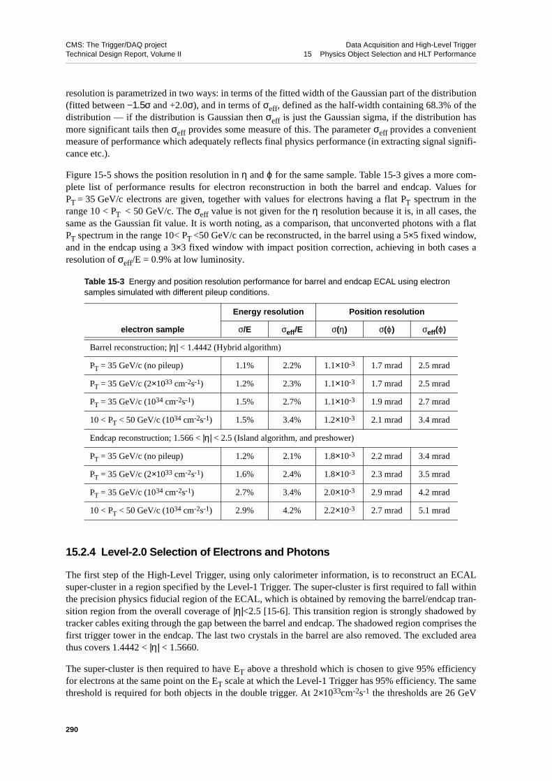
CMS: The Trigger/DAQ project Data Acquisition and High-Level TriggerTechnical Design Report, Volume II 15 Physics Object Selection and HLT Performance
resolution is parametrized in two ways: in terms of the fitted width of the Gaussian part of the distribution(fitted between −1.5σ and +2.0σ), and in terms of σeff, defined as the half-width containing 68.3% of thedistribution — if the distribution is Gaussian then σeff is just the Gaussian sigma, if the distribution hasmore significant tails then σeff provides some measure of this. The parameter σeff provides a convenientmeasure of performance which adequately reflects final physics performance (in extracting signal signifi-cance etc.).
Figure 15-5 shows the position resolution in η and ϕ for the same sample. Table 15-3 gives a more com-plete list of performance results for electron reconstruction in both the barrel and endcap. Values forPT = 35 GeV/c electrons are given, together with values for electrons having a flat PT spectrum in therange 10 < PT < 50 GeV/c. The σeff value is not given for the η resolution because it is, in all cases, thesame as the Gaussian fit value. It is worth noting, as a comparison, that unconverted photons with a flatPT spectrum in the range 10< PT <50 GeV/c can be reconstructed, in the barrel using a 5×5 fixed window,and in the endcap using a 3×3 fixed window with impact position correction, achieving in both cases aresolution of σeff/E = 0.9% at low luminosity.
15.2.4 Level-2.0 Selection of Electrons and Photons
The first step of the High-Level Trigger, using only calorimeter information, is to reconstruct an ECALsuper-cluster in a region specified by the Level-1 Trigger. The super-cluster is first required to fall withinthe precision physics fiducial region of the ECAL, which is obtained by removing the barrel/endcap tran-sition region from the overall coverage of |η|<2.5 [15-6]. This transition region is strongly shadowed bytracker cables exiting through the gap between the barrel and endcap. The shadowed region comprises thefirst trigger tower in the endcap. The last two crystals in the barrel are also removed. The excluded areathus covers 1.4442 < |η| < 1.5660.
The super-cluster is then required to have ET above a threshold which is chosen to give 95% efficiencyfor electrons at the same point on the ET scale at which the Level-1 Trigger has 95% efficiency. The samethreshold is required for both objects in the double trigger. At 2×1033cm-2s-1 the thresholds are 26 GeV
Table 15-3 Energy and position resolution performance for barrel and endcap ECAL using electronsamples simulated with different pileup conditions.
electron sample
Energy resolution Position resolution
σ/E σeff/E σ(η) σ(ϕ) σeff(ϕ)
Barrel reconstruction; |η| < 1.4442 (Hybrid algorithm)
PT = 35 GeV/c (no pileup) 1.1% 2.2% 1.1×10⁻³ 1.7 mrad 2.5 mrad
PT = 35 GeV/c (2×1033 cm-2s-1) 1.2% 2.3% 1.1×10⁻³ 1.7 mrad 2.5 mrad
PT = 35 GeV/c (1034 cm-2s-1) 1.5% 2.7% 1.1×10⁻³ 1.9 mrad 2.7 mrad
10 < PT < 50 GeV/c (1034 cm-2s-1) 1.5% 3.4% 1.2×10⁻³ 2.1 mrad 3.4 mrad
Endcap reconstruction; 1.566 < |η| < 2.5 (Island algorithm, and preshower)
PT = 35 GeV/c (no pileup) 1.2% 2.1% 1.8×10⁻³ 2.2 mrad 3.4 mrad
PT = 35 GeV/c (2×1033 cm-2s-1) 1.6% 2.4% 1.8×10⁻³ 2.3 mrad 3.5 mrad
PT = 35 GeV/c (1034 cm-2s-1) 2.7% 3.4% 2.0×10⁻³ 2.9 mrad 4.2 mrad
10 < PT < 50 GeV/c (1034 cm-2s-1) 2.9% 4.2% 2.2×10⁻³ 2.7 mrad 5.1 mrad
290

CMS: The Trigger/DAQ project Data Acquisition and High-Level TriggerTechnical Design Report, Volume II 15 Physics Object Selection and HLT Performance
for the single, and 14.5 GeV for the double. The corresponding thresholds at 1034 cm-2s-1 are 31 GeV and16.9 GeV. The rejection obtained from this cut on the transverse energy reconstructed in the ECAL isquite modest — about a factor of two on each object.
Some refinements of this Level-2.0 selection can be envisaged, but have not been used in the basic selec-tion procedure for which results are here presented. Firstly, the Level-2 selection uses cuts on purely ca-
Figure 15-4 Distribution of Emeas/Etrue for PT = 35 GeV/c electrons, a) in the barrel ECAL fully digitized withoutpileup, and reconstructed with the Hybrid super-clustering algorithm, b) the same distribution for electrons in theendcap, reconstructed with the Island super-clustering algorithm, and with preshower energy included.
Figure 15-5 Position resolution for PT = 35 GeV/c electrons in the barrel ECAL, fully digitized without pileup,and reconstructed with the Hybrid super-clustering algorithm.
0
1000
2000
3000
4000
5000
0.7 0.775 0.85 0.925 1 1.075 1.15
µ = 1.000
σGauss / µ = 1.06 %
σeff / µ = 2.24 %
Emeas / Etrue
electronspT = 35 GeV
Barrel
Eve
nts
0
1000
2000
3000
4000
5000
0.7 0.775 0.85 0.925 1 1.075 1.15
µ = 1.005
σGauss / µ = 1.23 %
σeff / µ = 2.11 %
Emeas / Etrue
electronspT = 35 GeV
Endcaps
Eve
nts
0
500
1000
1500
2000
2500
3000
-0.025 -0.0125 0 0.0125 0.025
σGauss = 1.7 mrad
σeff = 2.5 mrad
φmeas - φtrue (rad)
electronspT = 35 GeV
Barrel
Eve
nts
0
500
1000
1500
2000
2500
3000
-0.025 -0.0125 0 0.0125 0.025
σGauss = 1.1x10⁻³
σeff = 1.1x10⁻³
ηmeas - ηtrue
electronspT = 35 GeV
Barrel
Eve
nts
291

CMS: The Trigger/DAQ project Data Acquisition and High-Level TriggerTechnical Design Report, Volume II 15 Physics Object Selection and HLT Performance
lorimetric quantities — ECAL isolation and an H/E (hadronic/electromagnetic) cut — which could beapplied at an earlier stage. Secondly, a significant contribution to the transverse energy resolution comesfrom the lack of knowledge, at this stage, of the longitudinal vertex position. The contribution to the frac-tional ET resolution, as a function of η, due to a 1 σ shift if the vertex longitudinal position (5.3 cm) isshown in Figure 15-6. A small improvement in efficiency would be obtained by making the electronthreshold cuts in two stages: a looser cut at Level-2.0 followed by the full set of cuts at a later stage, afterthe pixel matching of Level-2.5 which gives a precise longitudinal vertex position.
15.2.5 Level-2.5: Matching of Super-clusters to Hits in the Pixel Detector
The matching of super-clusters reconstructed in the calorimeter to hits in the pixel detector takes advan-tage of the fact that the energy-weighted average impact point of an electron and the bremsstrahlung pho-tons it has radiated is precisely where a non-radiating electron would have impacted. It is this space-pointthat the position measurement of the super-cluster attempts to determine. This point can be propagatedback through the field to obtain an estimate of the direction of the electron at the vertex, and the hit posi-tions expected in the pixel detector. Since most of the tracker material lies after the pixel detector, mostelectrons do not radiate significantly before it, and most photon conversions take place after it. So match-ing hits are given by most electrons and by few photons.
Figure 15-6 Fractional ET resolution, as a function of η, induced by a 1 σ shift of the longitudinal vertex position.
Figure 15-7 Full pixel detector (high luminosity) with continuous lines pointing from the nominal vertex to theedges of the ECAL barrel and endcap, and dashed lines pointing from z = ± 15 cm.
0
1
2
0 0.5 1 1.5 2 2.5
∆pT/p
T (
%)
η
Measurement depth:Rbarrel = 136.5 c.m.Zendcap = 328.0 c.m.
η=1.5
η=2.5
zvtx = ± 15 cm
292

CMS: The Trigger/DAQ project Data Acquisition and High-Level TriggerTechnical Design Report, Volume II 15 Physics Object Selection and HLT Performance
The layout of the pixel system is shown in Figure 15-7. The continuous lines show the maximum η valuesof the ECAL barrel and endcaps and the dashed lines correspond to electrons generated z = ±15 cm awayfrom the nominal vertex. For the clusters at the ends of the ECAL barrel, pixel disks are needed as well asbarrel pixel layers. For endcap clusters the mix of pixel barrel and pixel disk hits depends on both thepseudorapidity and the z-vertex of the electron. With the currently simulated geometry there is a loss ofefficiency in the high |η| region of the ECAL endcap where, in some cases, the electron goes through onlyone pixel layer.
As described in Section 14.2.1, the outer barrel layer and the outermost endcap disks of the pixel detectorare “staged” and will not be present at start-up. The simulation of the HLT selection at low luminosity ismade by discarding pixel information in these layers.
The method proceeds as follows:
1. The electromagnetic cluster gives the energy and the position of the electron candidate. The trans-verse momentum is computed from the measured energy and position of the cluster. The expectedhit position on the pixel layers is estimated by propagating the electron inwards to the nominal ver-tex using the magnetic field map. A search area is defined in the innermost pixel layer. It is unre-stricted in z, and its width in φ (typically 40mrad) is the main parameter used to control thetightness of the pixel matching. The errors on the calculated hit positions are due to the spread in zof the vertex position and the precision of the j measurement in the calorimeter. At this stage the er-ror on the cluster ET measurement contributes very little to the uncertainty on the expected hit po-sition in the pixel detector.
2. If a compatible hit is found within the search area on the innermost pixel layer, a better estimate ofthe longitudinal (z) vertex position is obtained by interpolating the line from the cluster through thecorresponding hit to the beam line. Nominal values (0,0) for x and y coordinates of the vertex areassumed. If no hit is found in the search area of the innermost pixel layer, the search is repeated inthe next layer.
3. The track is propagated from the newly estimated vertex to the next pixel layer through the com-patible hit in the first (or second) layer. The dominating uncertainty, in the r-ϕ plane, now comesfrom the estimate of the ET of the electromagnetic cluster, and thus the radius of curvature of theelectron track. But this is a very small error since the distance from one pixel layer to the next isshort. Indeed, assuming a hit on the r = 4 cm layer, the distance between the hit predictions on ther = 11 cm layer for PT = 15 GeV/c and PT = 20 GeV/c electron would be 78 µm — less than thesize of a pixel. In the r-z plane, the main uncertainty comes from the vertex z.
4. If another compatible hit is found, the cluster is identified as an electron, if not, it is rejected as ajet. If there are no compatible hits in the current layer, there may be one more pixel layer left, andthe search is repeated there.
The search is made twice, once for each charge. In the first step of the search the electron and positronsearch areas can overlap, but in the second step, when a compatible hit is propagated to another pixel lay-er, the PT needed for the search areas of different charges to overlap is almost 1 TeV/c.
For low luminosity both the “staged” and full pixel detector configurations are investigated. Using the in-ner pixel layers alone results in a large inefficiency (≈7%) in the staged pixel configuration, so the low lu-minosity staged pixel detector algorithm supplements the pixel hits with hits found in the first silicon striplayer of the tracker, and regains some of the lost efficiency. More details of the Level-2.5 pixel matchingalgorithm are given in reference [15-7].
The rejection versus efficiency obtained from the Level-2.5 pixel matching is shown in Figure 15-8, at a)low luminosity (2×1033 cm-2s-1), and b) high luminosity (1034 cm-2s-1). The efficiency is calculated using
293

CMS: The Trigger/DAQ project Data Acquisition and High-Level TriggerTechnical Design Report, Volume II 15 Physics Object Selection and HLT Performance
an electron sample passing the Level-2.0 threshold. The rejection is calculated from the single electrontriggers in the jet background passing the Level-2.0 threshold, and refers to rejection from the electronstream. In practice, single and double photon streams are created by applying an ET threshold to theevents rejected by the pixel matching.
For the low luminosity case two different curves of the efficiency versus rejection, corresponding to thefull and staged pixel detector configurations, are shown in Figure 15-8(left).
The performance at high luminosity, shown in Figure 15-8(right), is very similar to the low luminosityperformance without staging with respect to electron efficiency, but there is a noticeable loss of rejectionpower which can be attributed to pileup hits. The high luminosity figure also shows the performance in amore restricted central region (|η|<2.1) where the efficiency is noticeably better. Although not shown inthe figure, the same is also true at low luminosity. The curves show seven connected points, in each casethe set of points corresponds to the same set of seven cuts in ∆ϕ.
15.2.6 Inclusion of Full Tracking Information: “Level-3” Selection
The Level-3 selection includes all further requirements needed to reach an acceptable rate to final offlinestorage. The full event information, including tracks, is available, but some of the cuts used — hadron-ic/electromagnetic energy fraction and calorimetric isolation — use only calorimetric information, andmight, in a fully optimized selection chain be made at an earlier stage.
15.2.6.1 Electrons
The Level-3 selection for electrons starts with electron track-finding, seeded by the Level-2.5 pixelmatch. To maintain high efficiency track-finding is made with very loose cut parameters. Cuts are thenmade on both E/P and on the distance between the super-cluster position and the extrapolated track posi-tion in the ECAL in the longitudinal coordinate, ∆η(track - cluster), which is only slightly distorted by
Figure 15-8 Rejection versus efficiency obtained from the Level-2.5 pixel matching. Left: at low luminosity(2×1033 cm-2s-1); the top curve shows the performance when the full pixel detector is used while the lower curveshows the performance for the staged pixel scenario (see text). Right: at high luminosity (1034 cm-2s-1); thelower curve is the nominal detector configuration; the top curve corresponds to |η|<2.1.
80
85
90
95
100
5 10 15 20 25
|η| < 2.1|η| < 2.5
Jet rejection
1034/cm2/s
e± effi
cien
cy [%
]
80
85
90
95
100
5 10 15 20 25Jet rejection
2x1033/cm2/s
e± effi
cien
cy [%
]
294
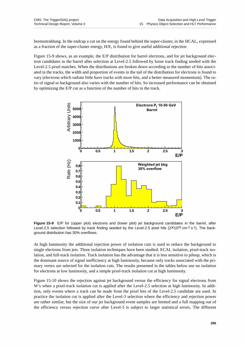
CMS: The Trigger/DAQ project Data Acquisition and High-Level TriggerTechnical Design Report, Volume II 15 Physics Object Selection and HLT Performance
bremsstrahlung. In the endcap a cut on the energy found behind the super-cluster, in the HCAL, expressedas a fraction of the super-cluster energy, H/E, is found to give useful additional rejection
Figure 15-9 shows, as an example, the E/P distribution for barrel electrons, and for jet background elec-tron candidates in the barrel after selection at Level-2.5 followed by loose track finding seeded with theLevel-2.5 pixel matches. When the distributions are broken down according to the number of hits associ-ated in the tracks, the width and proportion of events in the tail of the distribution for electrons is found tovary (electrons which radiate little have tracks with more hits, and a better measured momentum). The ra-tio of signal to background also varies with the number of hits. So increased performance can be obtainedby optimizing the E/P cut as a function of the number of hits in the track.
At high luminosity the additional rejection power of isolation cuts is used to reduce the background tosingle electrons from jets. Three isolation techniques have been studied: ECAL isolation, pixel-track iso-lation, and full-track isolation. Track isolation has the advantage that it is less sensitive to pileup, which isthe dominant source of signal inefficiency at high luminosity, because only tracks associated with the pri-mary vertex are selected for the isolation cuts. The results presented in the tables below use no isolationfor electrons at low luminosity, and a simple pixel-track isolation cut at high luminosity.
Figure 15-10 shows the rejection against jet background versus the efficiency for signal electrons fromW’s when a pixel-track isolation cut is applied after the Level-2.5 selection at high luminosity. In addi-tion, only events where a track can be made from the pixel hits of the Level-2.5 candidate are used. Inpractice the isolation cut is applied after the Level-3 selection where the efficiency and rejection powerare rather similar, but the size of our jet background event samples are limited and a full mapping out ofthe efficiency versus rejection curve after Level-3 is subject to larger statistical errors. The different
Figure 15-9 E/P for (upper plot) electrons and (lower plot) jet background candidates in the barrel, afterLevel-2.5 selection followed by track finding seeded by the Level-2.5 pixel hits (2×1033 cm-2 s-1). The back-ground distribution has 30% overflows.
0
1000
2000
3000
4000
5000
0 0.5 1 1.5 2 2.5 3E/P
Electrons PT 10-50 GeVBarrel
00.10.20.30.40.50.60.70.8
0 0.5 1 1.5 2 2.5 3
Weighted jet bkg30% overflow
E/P
Arb
itrar
y U
nits
Rat
e (H
z)
295

CMS: The Trigger/DAQ project Data Acquisition and High-Level TriggerTechnical Design Report, Volume II 15 Physics Object Selection and HLT Performance
points on the plot correspond to different cuts on the number of 3-hit pixel lines with PT > 1GeV/c foundwithin cones of different sizes.
15.2.6.2 Photons
Further ET thresholds, higher than those applied at Level-2.0, are applied to super-clusters of single anddouble triggers that fail the Level-2.5 pixel matching. The events passing these cuts form the photonstream. The double photon thresholds are asymmetric, chosen to be 5 GeV lower than the offline analysiscuts envisaged for the Standard Model H→γγ search [15-6]. The single photon thresholds are chosen togive an acceptable rate. Table 15-4 lists the thresholds and the rates before further Level-3 selection.
Background rejection is available using isolation and π0 rejection based on lateral shower shape. Trackisolation has the advantage that it is less sensitive to pileup at high luminosity, but to take this advantage avertex must be defined. Defining the longitudinal coordinate of the vertex is a significant issue for theH→γγ signal channel. For events where one or more of the photons has converted in the tracker, the tracksegment and the ECAL cluster will be used to locate the vertex. The vertices in the remaining events willbe found using algorithms that choose the track vertex associated with the largest track activity. These al-gorithms have not yet been incorporated into the High-Level Trigger selection.
Figure 15-10 Rejection against jet background versus the efficiency for electrons from Ws when a pixel-trackisolation cut is applied after the Level-2.5 selection at 1034 cm-2s-1.
Table 15-4 Photon stream thresholds and rates before additional Level-3 cuts.
Threshold Rate @ 2×1033 cm-2s-1 Rate @ 1034 cm-2s-1
Single photon ET > 80 GeV (2×1033)ET > 100 GeV (1034)
7 Hz10 Hz
Double photons ET1 > 35, ET
2 > 20 GeV 85 Hz 382 Hz
0.6
0.65
0.7
0.75
0.8
0.85
0.9
0.95
1
1.05
0 0.2 0.4 0.6 0.8 1 1.2
εpxl isol(QCD)
ε pxl i
sol(W
→eν
)
Rcone=0.2
Rcone=0.3
Rcone=0.4
Rcone=0.5
L=1034cm-2s-1
296
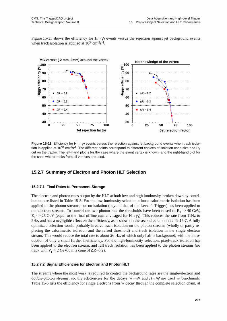
CMS: The Trigger/DAQ project Data Acquisition and High-Level TriggerTechnical Design Report, Volume II 15 Physics Object Selection and HLT Performance
Figure 15-11 shows the efficiency for H→γγ events versus the rejection against jet background eventswhen track isolation is applied at 1034cm-2s-1.
15.2.7 Summary of Electron and Photon HLT Selection
15.2.7.1 Final Rates to Permanent Storage
The electron and photon rates output by the HLT at both low and high luminosity, broken down by contri-bution, are listed in Table 15-5. For the low-luminosity selection a loose calorimetric isolation has beenapplied to the photon streams, but no isolation (beyond that of the Level-1 Trigger) has been applied tothe electron streams. To control the two-photon rate the thresholds have been raised to ET
1 > 40 GeV,ET
2 > 25 GeV (equal to the final offline cuts envisaged for H→γγ). This reduces the rate from 11Hz to5Hz, and has a negligible effect on the efficiency, as is shown in the second column in Table 15-7. A fullyoptimized selection would probably involve track isolation on the photon streams (wholly or partly re-placing the calorimetric isolation and the raised threshold) and track isolation in the single electronstream. This would reduce the total rate to about 26 Hz, of which only half is background, with the intro-duction of only a small further inefficiency. For the high-luminosity selection, pixel-track isolation hasbeen applied to the electron stream, and full track isolation has been applied to the photon streams (notrack with PT > 2 GeV/c in a cone of ∆R=0.2).
15.2.7.2 Signal Efficiencies for Electron and Photon HLT
The streams where the most work is required to control the background rates are the single-electron anddouble-photon streams, so, the efficiencies for the decays W→eν and H→γγ are used as benchmark.Table 15-6 lists the efficiency for single electrons from W decay through the complete selection chain, at
Figure 15-11 Efficiency for H → γγ events versus the rejection against jet background events when track isola-tion is applied at 1034 cm-2s-1. The different points correspond to different choices of isolation cone size and PTcut on the tracks. The left-hand plot is for the case where the event vertex is known, and the right-hand plot forthe case where tracks from all vertices are used.
MC vertex: (-2 mm, 2mm) around the vertex
Jet rejection factor
Hig
gs
effi
cien
cy [
%]
∆R = 0.2
∆R = 0.3
∆R = 0.4
30
40
50
60
70
80
90
100
0 25 50 75 100
No knowledge of the vertex
Jet rejection factor
Hig
gs
effi
cien
cy [
%]
∆R = 0.2
∆R = 0.3
∆R = 0.4
30
40
50
60
70
80
90
100
0 25 50 75 100
297

CMS: The Trigger/DAQ project Data Acquisition and High-Level TriggerTechnical Design Report, Volume II 15 Physics Object Selection and HLT Performance
2×1033cm-2s-1 and at 1034 cm-2s-1. Events are preselected requiring the generated electrons to be withinthe ECAL fiducial region of |η| < 2.5, with the region 1.4442 <|η| < 1.5660 excluded. The geometric ac-ceptance is approximately 60% and is not included in the efficiency. The second and fourth columns listthe efficiencies for electrons that have PT greater than the Level-1 and Level-2 95% efficiency point.
The efficiencies at 1034 cm-2s-1 are only slightly lower. The main difference comes from the loss due tothe additional isolation cuts — typically a 5% loss per object.
Table 15-7 lists the efficiency for H→γγ for a Higgs with mass MH = 115 GeV/c2 through the completeselection chain, at 2×1033cm−2s−1. As in the previous Table, events are preselected, requiring that thegenerated photons fall within the ECAL fiducial region. The geometric acceptance is 65%. The secondcolumn shows the efficiency for events where the two generated photons satisfy, in addition, the cuts cur-rently assumed for offline analysis in this channel — PT
1 > 40 GeV/c, PT2 > 25 GeV/c.
15.2.7.3 CPU Usage for Electron and Photon HLT
Table 15-8 shows the CPU usage of the HLT selection, benchmarked on 1GHz Pentium III processor, forjet background events at low luminosity. At high luminosity the time taken for the unoptimized globalsearch for ECAL clusters at Level-2.0 is greatly increased and the overall total CPU time per Level-1event, at a luminosity of 1034 cm-2s-1 is about three times as large, as at 2×1033 cm-2s-1. Preliminary re-sults indicate that this clustering time can be reduced by a factor ~10 using regional reconstruction.
Table 15-5 Electron and photon rates output by the HLT at low and high luminosity.
2x1033cm-2s-1 1034cm-2s-1
Signal Background Total Signal Background Total
Single electron W→eν: 10Hz π±/π0 overlap: 5Hzπ0 conversions: 10Hz
b/c→e: 8Hz
33Hz W→eν: 35Hz π±/π0 overlap: 15Hzπ0 conversions: 19Hz
b/c→e: 6Hz
75Hz
Double electron Z→ee: 1Hz ~0 1Hz Z→ee: 4Hz ~0 4Hz
Single photon 2Hz 2Hz 4Hz 4Hz 3Hz 7Hz
Double photon ~0 5Hz 5Hz ~0 8Hz 8Hz
TOTAL: 43Hz 94Hz
Table 15-6 Ffficiency for electrons from W decay through the complete selection chain.
Low luminosity High luminosity
All fiducial electrons
Fiducial electrons with PT > 29 GeV/c
All fiducial electrons
Fiducial electrons with PT > 34 GeV/c
Level-1 63.2% 87.2% 51.1% 83.2%
Level-2 88.8% 99.4% 82.9% 99.3%
Level-2.5 93.1% 94.6% 92.8% 94.1%
Level-3 81% 82% 77% 78%
HLT (Level-2 to Level-3) 67% 77% 59% 73%
298

CMS: The Trigger/DAQ project Data Acquisition and High-Level TriggerTechnical Design Report, Volume II 15 Physics Object Selection and HLT Performance
Two steps are not included in the values listed in Table 15-8. The sub-detector data will have to bechecked for consistency and formatted. This will be done, initially, only for data in the region of the Lev-el-1 Trigger. The time required for this step has not been measured yet, however there is no reason to ex-pect that it will contribute very significantly to the total. The energy in the ECAL crystals has then to bereconstructed from the time samplings. In the Monte Carlo this is done for the entire detector, and thetime taken (0.8 s) is dominated by the pre-shower detector (0.5s). Since only data in a small region needbe reconstructed, and the formatted data can be sub-divided more finely than a ReadOut unit, the time re-quired for this step will be 100 times less. Figure 15-12 shows the distribution of the total CPU time takenfor the full HLT processing of e/γ triggers at 2×1033cm-2s-1.
Table 15-7 Efficiency for H→γγ (MH=115 GeV/c2) through the complete selection chain, at 2×1033 cm-2s-1.
Both photons in fiducial region Photons passing offline PT cuts
Level-1 90.8% 92.3%
Level-2 98.7% 99.4%
Level-2.5 93.4% 99.1%
Level-3 92% 92%
Overall (Level-1 × HLT) 77% 83.7%
Table 15-8 CPU usage of the HLT selection at 2×1033cm-2s-1.
HLT level Mean CPU time (ms)
Level-2.0 154 /Level-1 event
Level-2.5 32 /Level-2 event
Level-3 100 /Level-2.5 event
Total 162 ms/Level-1 event
Figure 15-12 Distribution of total CPU time taken by the HLT for the selection of electrons and photonsat 2×1033cm-2s-1. The inset shows the same time plotted against log(t), and with a Gaussian in log(t) fitted to it.
0
50
100
150
200
250
0 0.1 0.2 0.3 0.4 0.5 0.6 0.7 0.8 0.9 1Time (s)
Even
ts
Mean = 162 ms/Level-1
0
50
100
150
200
250
-4 -3 -2 -1 0
55.22 / 52Constant 177. 5Mean -1.828Sigma 0.3607
log(t)
299

CMS: The Trigger/DAQ project Data Acquisition and High-Level TriggerTechnical Design Report, Volume II 15 Physics Object Selection and HLT Performance
15.3 Muon Identification
The muon selection for the High-Level Trigger proceeds in two steps: firstly, muons are reconstructed inthe muon chambers, which confirms the Level-1 decision and refines the PT measurement using moreprecise information; secondly, the muon trajectories are extended into the tracker, which further refinesthe PT measurement. After each step, isolation is applied to the muon candidates the calorimeter beingused after the first step and the tracker after the second.
The muon track reconstruction algorithm used by the High-Level Trigger is seeded by the muon candi-dates found by the Level-1 Global Muon Trigger (no more than four), including those candidates that didnot necessarily lead to a Level-1 accept by the Global Trigger. The algorithm uses the reconstructed hitsbuilt from the digitized signals in the muon system, and constructs tracks according to the Kalman filtertechnique, as described in Section 14.4.1. The resulting trajectories are used to validate the Level-1 deci-sion as well as to refine the muon measurement in this “Level-2” muon selection. The basis of the “Lev-el-3” muon selection is to add silicon tracker hits to the muon trajectory, thus greatly improving the muonmomentum measurement and sharpening the trigger threshold. Isolation criteria can be applied to themuon candidates to provide additional rejection: at Level-2 using the calorimetric energy sum in a conearound the muon, and at Level-3 using the number of pixel tracks in a region around the projected muontrajectory. This suppresses non-prompt muons from b, c, π, and K decays.
Sections 15.3.1 and 15.3.2 describe the general “tools” that are available to form the muon HLT: muon re-construction and isolation. Section 15.3.3 describes how these tools are used to form the muon HLT, in-cluding additional cuts to suppress fake triggers. Finally, Section 15.3.4 describes the efficiency, rate, andCPU usage of the muon HLT.
15.3.1 Muon Reconstruction
15.3.1.1 Muon Standalone Reconstruction and Level-2 Selection
Reconstructed track segments from the muon chambers are used for muon identification and selection at“Level-2”. The state vectors (track position, momentum and direction) associated with the segmentsfound in the innermost chambers are propagated outwards through the iron yoke using the GEANE pack-age [15-8], which takes into account the muon energy loss in the material, the effect of the multiple scat-tering, and the non-constant magnetic field in the muon system. The estimate of the momentum from theLevel-1 Global Muon Trigger is used initially for the track propagation in the magnetic field. The predict-ed state vector at the next measurement surface is compared with existing measured points and updatedaccordingly using a Kalman filter technique. In the barrel chambers, reconstructed track segments areused as measurements in the Kalman filter procedure; in the endcap chambers, where the magnetic field isinhomogeneous, it is the individual reconstructed hits belonging to the track segments that are used. Re-constructed hits from RPC chambers are also included. The procedure is iterated until the outermostmeasurement surface of the muon system is reached, at which point a constrained fit to the track parame-ters, working from the outside in, is performed under the assumption that the muon candidate originatedfrom the interaction region (defined by the beam spot size: σxy=15 µm and σz=5.3 cm). In both the for-ward and backward propagations just described, a measurement is not added to the muon trajectory if itscontribution to the total χ2 exceeds 25. The resulting track parameters, propagated inward to the collisionvertex, are used to reject or accept the event for further Level-3 processing. More details on thisstand-alone muon reconstruction can be found in reference [15-9].
300

CMS: The Trigger/DAQ project Data Acquisition and High-Level TriggerTechnical Design Report, Volume II 15 Physics Object Selection and HLT Performance
Figure 15-13 shows the resolution of the transverse momentum determined by the Level-2 constrained fitas expressed by the distribution of the quantity (1/PT
rec −1/PTgen) / (1/PT
gen), where PTgen and PT
rec arethe generated and reconstructed transverse momenta, respectively. Muons from W decays at high lumi-nosity form the reference sample. The distributions are broken up into three pseudorapidity intervals: bar-rel (|η|<0.8), overlap (0.8<|η|<1.2) and endcap (1.2<|η|<2.1). In these three regions, the fitted PTresolutions are 10%, 15%, and 16%, respectively.
15.3.1.2 Inclusion of Tracker Information and Level-3 Selection
The “Level-3” muon reconstruction consists of extending the muon trajectories to include hits in the sili-con tracker system. Starting from a Level-2 reconstructed muon, the muon trajectory is extrapolated fromthe innermost muon station to the outer tracker surface, taking into account the muon energy loss in thematerial and the effect of multiple scattering. As with Level-2, the GEANE package is currently used forthe propagation through the iron and calorimeters. Silicon layers compatible with the muon trajectory arethen determined, and a region of interest within them is defined to perform regional track reconstruction.The determination of the region of interest is based on the track parameters and uncertainties of the ex-trapolated Level-2 muon trajectory, obtained with the assumption that the muon originates from the inter-action point as described in the previous section. This has a strong impact on the reconstructionefficiency, fake rate, and CPU reconstruction time: well measured muons are reconstructed faster andwith higher efficiency than poorly measured ones.
Inside the region of interest, initial candidates for the muon trajectory (regional seeds) are built from pairsof reconstructed hits. The two hits forming a seed must come from two different tracker layers, and allcombinations of compatible pixel and double-sided silicon strip layers are used in order to achieve highefficiency. In addition, a beam spot constraint is applied to muon candidates above a given transverse mo-mentum threshold to obtain initial trajectory parameters.
Starting from the regional seeds, a track reconstruction algorithm based on the Kalman filter techniquedescribed in Section 14.4.1, is used to reconstruct tracks inside the selected region of interest. The trackreconstruction algorithm consists of the following steps: trajectory building (seeded pattern recognition),trajectory cleaning (resolution of ambiguities) and trajectory smoothing (final fit). In the first step, the tra-jectory builder transforms each seed into a set of trajectories. Starting from the innermost layer, the trajec-tory is propagated to the next tracker layer that is reachable, and updated with compatible measurements
Figure 15-13 Distribution of (1/PTrec -1/PT
gen) / (1/PTgen) where PT
gen and PTrec are the generated and Level-2
reconstructed transverse momenta respectively, shown in three pseudorapidity intervals: a) |η| < 0.8,b) 0.8 < |η| < 1.2, and c) 1.2 < |η| < 2.1.
-1 -0.5 0 0.5 10
200
400
600
800
1000
1200
(a)
-1 -0.5 0 0.5 10
50
100
150
200
250
300
350
400
(b)
-1 -0.5 0 0.5 10
100
200
300
400
500
600
700
800
(c)
301

CMS: The Trigger/DAQ project Data Acquisition and High-Level TriggerTechnical Design Report, Volume II 15 Physics Object Selection and HLT Performance
found on that layer. In the second step, the trajectory cleaner resolves ambiguities between multiple tra-jectories that may result from a single seed on the basis of the number of hits and the chi-square of the fit.In the final step, all reconstructed tracks are fit once again with reconstructed hits in the muon chambersincluded from the original Level-2 reconstructed muon, and selected on the basis of a chi-square cut.
Figure 15-14 shows the resolution of the transverse momentum determined by the Level-3 constrained fitas expressed by the distribution of the quantity (1/PT
rec −1/PTgen) / (1/PT
gen), where PTgen and PT
rec arethe generated and reconstructed transverse momenta, respectively. Muons from W decays at high lumi-nosity are used as the reference sample. The distributions are broken up into three pseudorapidity inter-vals: barrel (|η|<0.8), overlap (0.8<|η|<1.3) and endcap (1.3<|η|<2.1). In these three regions, the fitted PTresolutions are 1.0%, 1.4%, and 1.7%, respectively. The improvement over the stand-alone muon meas-urement from Level-2 is substantial.
The efficiency of the Level-3 tracking algorithm relative to the Level-2 selection is shown in Fig. 15-15as a function of η for single muons with PΤ>10 GeV/c and no pile-up. The muons were generated flat inPT up to 100 GeV/c. The algorithmic efficiency is typically 99%, except in the pseudorapidity interval0.8<|η|<1.2, where the DT and CSC systems overlap and the efficiency is about 97%.
15.3.2 Muon Isolation
The integrated rate of muons at LHC is dominated by muons from b, c, K, and π decays, as shown inFigure 14-1. These muons are generally accompanied by other nearby particles, so they can be suppressedby isolation cuts.
Three isolation techniques have been studied. The first (calorimeter isolation) is based on the standardtechnique of summing the calorimeter energy in a cone around the muon, and can be used with thestand-alone muon reconstruction at Level-2. However, as it is based on the calorimeter, this technique be-comes less effective at high luminosity as more pile-up is included in the sum. The second technique (pix-el isolation) is based on the partial reconstruction of tracks in the silicon pixel detector; in this case,isolation is determined on the basis of the sum of the transverse momenta of the tracks in a cone aroundthe muon. This method, which can be applied when tracker information is included at Level-3, is less sen-sitive to pile-up, as only tracks originating from the same collision vertex are considered. However, it re-
Figure 15-14 Distribution of (1/PTrec -1/PT
gen) / (1/PTgen) where PT
gen and PTrec are the generated and Level-3
reconstructed transverse momenta, respectively, shown in three pseudorapidity intervals: a) |η| < 0.8,b) 0.8 < |η| < 1.2, and c) 1.2 < |η| < 2.1.
-0.1 -0.05 0 0.05 0.10
200
400
600
800
1000 (a)
-0.1 -0.05 0 0.05 0.10
50
100
150
200
250
300
350
400
(b)
-0.1 -0.05 0 0.05 0.10
100
200
300
400
500
600
700
800
(c)
302

CMS: The Trigger/DAQ project Data Acquisition and High-Level TriggerTechnical Design Report, Volume II 15 Physics Object Selection and HLT Performance
quires the reconstruction of three pixel hits out of the three layers in the pixel detector for every track; forthis reason, it is sensitive to inefficiencies and may not be useful in staging scenarios where only two pix-el layers are installed. The third technique, tracker isolation, uses full tracks reconstructed regionally. Thismethod is more robust than pixel isolation, but is more time consuming especially at high luminosity.
For all three techniques, cones are defined by the condition ∆R ≤ ∆Rmax, where ,with ∆η and ∆φ the distances from the muon direction in pseudorapidity and azimuthal angle, respective-ly. The ΣΕΤ deposited in the cone in the case of calorimeter isolation or the ΣPΤ of tracks in the cone inthe case of pixel and tracker isolation are computed after subtracting the muon contribution (veto value)and compared with a predefined threshold. For each algorithm, both the cone size and the thresholds arechosen by maximising the rejection for a reference background sample while keeping the efficiency for areference signal sample above a given nominal value (nominal efficiency). The threshold is determinedindependently in 52 bins in η, in order to guarantee a flat signal efficiency as a function of η.
The rejection power of muon isolation algorithms depends on the PT of the muon, since low-PT muons areusually accompanied by low energy jets that may be below the isolation energy or momentum threshold.This is particularly relevant at Level-2, where the feed-through of low-PT muons contaminates the PTspectrum even for high thresholds. To exclude these muons, the reference background sample is definedas a sample of minimum-bias events containing only muons with PT above 22 GeV/c (16 GeV/c) for high(low) luminosity. The direct W→µν decay is used as reference signal since it contains well isolated muonswith adequate PT spectrum.
The result of the optimisation procedure is that for any predefined nominal efficiency value a cone size ischosen, with thresholds defined in bins of pseudorapidity. For all three isolation techniques, typical valuesof the optimal cone size ∆Rmax vary from 0.2 to 0.3.
The main features of the three isolation algorithms are briefly described in the following sections. A de-tailed description can be found in reference [15-10].
Figure 15-15 Algorithmic efficiency of the Level-3 tracking algorithm as a function of η for single muons gener-ated flat over 10 < PT < 100 GeV/c. No pile-up was included.
µ| η |0 0.5 1 1.5 2 2.5
Eff
icie
ncy
0.8
0.82
0.84
0.86
0.88
0.9
0.92
0.94
0.96
0.98
1
∆R ∆η( )2 ∆φ( )2+=
303

CMS: The Trigger/DAQ project Data Acquisition and High-Level TriggerTechnical Design Report, Volume II 15 Physics Object Selection and HLT Performance
15.3.2.1 Calorimeter Isolation
The calorimeter isolation algorithm uses the muon direction at the impact point for the definition of thecone axis. The extraction of the energy deposits is done independently in the ECAL and the HCAL. Thetotal energy is obtained as a weighted sum, ET = α ET
ECAL + ETHCAL, where α ≈ 1.5 is found to be an op-
timum value for the isolation technique. Thresholds on E and ET in individual ECAL crystals and HCALtowers are applied in order to reject noise and pile-up deposits. The energy deposit in a small cone aroundthe extrapolated position of the muon on the ECAL/HCAL boundary is used as veto value and subtractedfrom the measurement in the cone. Thresholds on the summed ET vary from 6.5 to 9 GeV for typical conesizes of 0.2.
15.3.2.2 Pixel Isolation
A pixel reconstruction algorithm looks for pixel hits compatible with tracks with transverse momenta aslow as 1 GeV/c. The track candidates are used to fit primary vertices; track candidates with no associationto reconstructed vertices are rejected. The algorithm returns a list of vertices with the correspondingtracks and their momenta. All pixel tracks contributing to the ΣPΤ in the cone are required to come fromthe same primary vertex as the Level-3 muon, thus reducing the effect of pile-up. The veto value is de-fined as the PT of the muon candidate, i.e. of the pixel track closest in direction to the muon, within∆R<0.015. Thresholds on the summed PT vary from 1.8 to 3.8 GeV/c for typical cone sizes of 0.2. Thepixel isolation algorithm can also be applied to Level-2 muon candidates, but because the muon trajectoryis less well determined than Level-3 candidates, the primary vertex requirement must be dropped and thecone size increased. The performance of the isolation algorithm is therefore different at Level-2 than atLevel-3.
15.3.2.3 Tracker Isolation
The tracker isolation algorithm is based on the ΣPΤ of tracks reconstructed in a cone around the directionof the Level-3 muon, neglecting the contribution from the muon itself. Tracks are reconstructed using re-gional tracking, i.e. track seeds are created using pairs of pixel hits in a region of interest. The region isdefined by a vertex constraint, the minimum transverse momentum for the tracks to be reconstructed aswell as a constrain on the track direction at the vertex. Thresholds on the summed PT varied from 2.0 to3.0 GeV/c for typical cone sizes of 0.2.
15.3.2.4 Performance
A general investigation of the isolation efficiency for signal muons and rejection of background is report-ed here, whereas the performance with respect to specific Level-1 and Level-2 triggers is included in Sec-tions 15.3.3 and 15.3.4. The isolation optimisation procedure guarantees by construction that theefficiency for the reference signal (W→µν events) is flat as a function of the pseudorapidity and equal to(or greater than) the chosen nominal efficiency. The efficiency for the background depends on the PT ofthe muon, as shown in Fig. 15-16a for the high luminosity case when the efficiency for the reference sig-nal is set to 97%. To show the performance of isolation algorithms, it is therefore necessary to specify thebackground sample and the minimum generated muon PT to be taken into account. This is particularly rel-evant for the Level-2 calorimeter isolation algorithm. In this case, the rate is dominated, for any PT thresh-old, by the feed-through of very low-PT muons, which cannot be rejected by the isolation algorithms butshould be rejected by the refined PT threshold at Level-3. Figure 15-16b shows the rejection power of theisolation algorithms, expressed as the efficiency for background muons in minimum-bias events withPT
gen>22 GeV/c at high luminosity, as a function of the pseudorapidity of the muon.
304
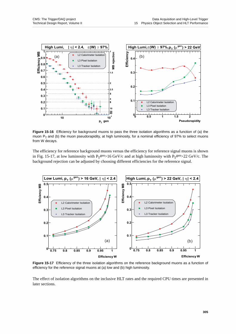
CMS: The Trigger/DAQ project Data Acquisition and High-Level TriggerTechnical Design Report, Volume II 15 Physics Object Selection and HLT Performance
The efficiency for reference background muons versus the efficiency for reference signal muons is shownin Fig. 15-17, at low luminosity with PT
gen>16 GeV/c and at high luminosity with PTgen>22 GeV/c. The
background rejection can be adjusted by choosing different efficiencies for the reference signal.
The effect of isolation algorithms on the inclusive HLT rates and the required CPU times are presented inlater sections.
Figure 15-16 Efficiency for background muons to pass the three isolation algorithms as a function of (a) themuon PT and (b) the muon pseudorapidity, at high luminosity, for a nominal efficiency of 97% to select muonsfrom W decays.
Figure 15-17 Efficiency of the three isolation algorithms on the reference background muons as a function ofefficiency for the reference signal muons at (a) low and (b) high luminosity.
Pseudorapidity0 0.5 1 1.5 2
Effic
ienc
y
0
0.1
0.2
0.3
0.4
L2 Calorimeter IsolationL3 Pixel IsolationL3 Tracker Isolation
) > 22 GeVgenµ(Tp
(a) (b)
p gen10 102
Effic
ienc
y M
B
0
0.1
0.2
0.3
0.4
0.5
0.6
0.7
0.8
0.9
1L2 Calorimeter Isolation
L3 Pixel Isolation
L3 Tracker Isolation
| < 2.4,η| 97%≥ε(W) High Lumi,
MB
reje
ctio
n1
1.5
2
2.5
33
455
102040
(a)
T
High Lumi, 97%,≥ε(W)
Efficiency W
0.75 0.8 0.85 0.9 0.95 1
Effic
ienc
y M
B
0
0.1
0.2
0.3
0.4
0.5
L2 Calorimeter Isolation
L3 Pixel Isolation
L3 Tracker Isolation
| < 2.4η) > 16 GeV, | genµ (TpLow Lumi,
Efficiency W
0.75 0.8 0.85 0.9 0.95 1
Effic
ienc
y M
B
0
0.1
0.2
0.3
0.4
0.5
L2 Calorimeter Isolation
L3 Pixel Isolation
L3 Tracker Isolation
(a) (b)
| < 2.4η) > 22 GeV, | genµ (TpHigh Lumi,
305

CMS: The Trigger/DAQ project Data Acquisition and High-Level TriggerTechnical Design Report, Volume II 15 Physics Object Selection and HLT Performance
15.3.3 Muon HLT Selection
Here we describe a prototype inclusive muon trigger based on the reconstruction and isolation tools dis-cussed above to demonstrate the performance possible in the muon HLT. Other combinations of cuts arealso possible, as are more sophisticated and more exclusive triggers.
15.3.3.1 Single-muon HLT Selection
A single muon inclusive trigger is formed from the following requirements. At Level-1, low quality CSCtracks must be matched with RPC tracks by the Global Muon Trigger (Section F.2.5) in order to ensure awell-measured PT. At Level-2, a muon must be reconstructed in the muon system and have a valid extrap-olation to the collision vertex. In the barrel region, at least one DT track segment reconstructed as de-scribed in Chapter 13 is required, and the sum of the number of DT segments and RPC hits must exceedthree. At Level-3, a muon must have more than 5 silicon hits in total from the pixels and silicon strips.
The overall efficiency for muons to pass the Level-1 through Level-3 single muon trigger criteria cumula-tively as a function of the generated η is shown in Fig. 15-18. Muons were generated flat in the intervals5<PT<100 GeV/c and |η|<2.1 without any pile-up. The average combined Level-1 through Level-3 effi-ciency without any requirements on the reconstructed PT is 97%, but is lower in some particular regionsbecause of gaps in the geometrical coverage of the chambers.
The efficiency turn-on curves as a function of the generated PT for several different PT thresholds areshown in Fig. 15-19. The efficiency shown is the cumulative Level-1 through Level-3 efficiency. Thethreshold at each trigger level is defined at 90% efficiency (relative to the plateau efficiency), and it canbe seen that the improved PT resolution at each successive level sharpens the turn-on curve. The efficien-cy at Level-3 for high PT muons varies from 97% (no threshold) to 90% (PT>40 GeV/c).
Additionally, for the HLT trigger, Level-2 muon candidates must satisfy the calorimeter isolation criteriaat the 97% efficiency point for the reference signal. At Level-3, candidates must satisfy the tracker and
Figure 15-18 Cumulative efficiency for single muons to pass the Level-1 (solid), Level-2 (dashed), and Level-3(dotted) triggers as a function of the generated muon pseudo-rapidity. No thresholds on PT are applied. Note thesuppressed zero on the y-axis. The dips at |η| ~ 0.3 and 0.8 are due to gaps in the muon chamber coverage.
|µη|0 0.5 1 1.5 2 2.5
Effic
ienc
y
0.86
0.88
0.9
0.92
0.94
0.96
0.98
1
|µη|0 0.5 1 1.5 2 2.5
Effic
ienc
y
0.86
0.88
0.9
0.92
0.94
0.96
0.98
1
306

CMS: The Trigger/DAQ project Data Acquisition and High-Level TriggerTechnical Design Report, Volume II 15 Physics Object Selection and HLT Performance
pixel isolation criteria (hereafter collectively referred to as “tracker isolation” in the figures that follow)both at the 97% efficiency point for the reference signal.
The single muon trigger rates as a function of the PT threshold are shown in Figure 15-20 for both low lu-minosity (L=2×1033 cm-2s-1) and high luminosity (L=1034 cm-2s-1). The rates are shown separately forLevel-1, Level-2, and Level-3, with and without isolation applied at Levels 2 and 3. Also shown is thesingle muon rate that was generated in the simulation. At low luminosity, the Level-3 inclusive sin-gle-muon trigger rate can be reduced to 30 Hz with a PT threshold of 18 GeV/c when the isolation criteriaare applied. The rate is about 100 Hz without isolation at Level-3 for the same threshold. At high lumi-nosity, a threshold of 38 GeV/c reduces the single-muon Level-3 rate to 30 Hz with isolation (50 Hz with-out isolation), and a threshold of 31 GeV/c yields a rate of 50 Hz (100 Hz without isolation). The reasonwhy isolation achieves less rejection at higher thresholds can be seen in Fig. 15-21, which shows the con-tributions to the Level-3 trigger rate at high luminosity from all sources of muons before and after all iso-lation criteria have been applied. The isolation criteria strongly suppress the contributions from b, c, K,and π decays. This reduces the HLT rate less at high thresholds, however, where the single-muon rate isdominated by W→µν decays. After the isolation criteria, W decays account for 50% (80%) of the inclu-sive single-muon rate for a threshold of 18 GeV/c (31 GeV/c) for low and high luminosity, respectively.
The efficiency of the HLT single-muon trigger to select W→µν and tt→µ+X events, where one W→µνdecay is required in the latter, is shown in Figure 15-22 as a function of the PT threshold at low luminosi-ty. Thresholds are defined as the PT value for which the efficiency for muons is 90% of the maximum at-tainable efficiency. Approximately 70% of both the W and top quark decays that occur in the fiducialregion |η|<2.1 are recorded by the isolated single-muon trigger for a PT threshold of 18 GeV/c. The effi-ciencies are 42% (53%) for W (top) decays for a PT threshold of 31 GeV/c.
Figure 15-19 Cumulative efficiency for single muons to pass the Level-1 (solid), Level-2 (dashed), and Level-3(dotted) triggers as a function of the generated PT for several trigger thresholds: a) PT > 10 GeV/c,b) PT > 20 GeV/c, c) PT > 30 GeV/c, and d) PT > 40 GeV/c.
Pt [GeV/c]0 10 20 30 40 50 60 70 80
Eff
icie
ncy
0
0.1
0.2
0.3
0.4
0.5
0.6
0.7
0.8
0.9
1
a)
Pt [GeV/c]0 10 20 30 40 50 60 70 80
Eff
icie
ncy
0
0.1
0.2
0.3
0.4
0.5
0.6
0.7
0.8
0.9
1
b)
Pt [GeV/c]0 10 20 30 40 50 60 70 80
Eff
icie
ncy
0
0.1
0.2
0.3
0.4
0.5
0.6
0.7
0.8
0.9
1
c)
Pt [GeV/c]0 10 20 30 40 50 60 70 80
Eff
icie
ncy
0
0.1
0.2
0.3
0.4
0.5
0.6
0.7
0.8
0.9
1
d)
307
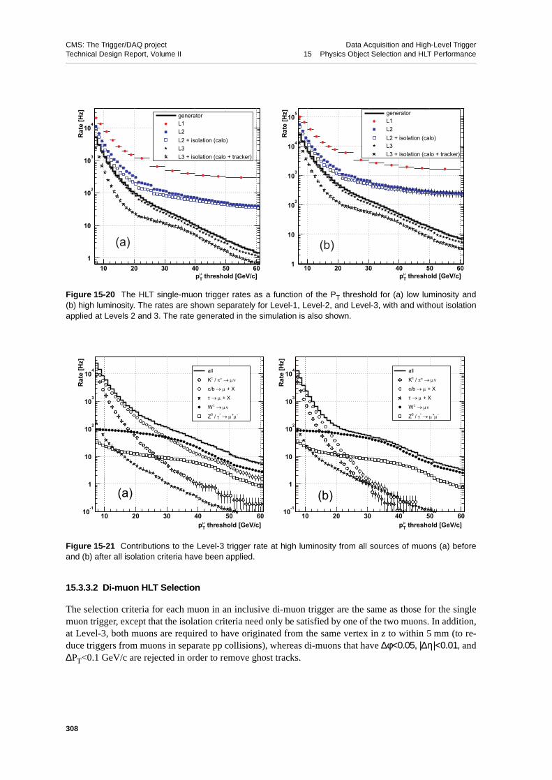
CMS: The Trigger/DAQ project Data Acquisition and High-Level TriggerTechnical Design Report, Volume II 15 Physics Object Selection and HLT Performance
15.3.3.2 Di-muon HLT Selection
The selection criteria for each muon in an inclusive di-muon trigger are the same as those for the singlemuon trigger, except that the isolation criteria need only be satisfied by one of the two muons. In addition,at Level-3, both muons are required to have originated from the same vertex in z to within 5 mm (to re-duce triggers from muons in separate pp collisions), whereas di-muons that have ∆φ<0.05, |∆η|<0.01, and∆PT<0.1 GeV/c are rejected in order to remove ghost tracks.
Figure 15-20 The HLT single-muon trigger rates as a function of the PT threshold for (a) low luminosity and(b) high luminosity. The rates are shown separately for Level-1, Level-2, and Level-3, with and without isolationapplied at Levels 2 and 3. The rate generated in the simulation is also shown.
Figure 15-21 Contributions to the Level-3 trigger rate at high luminosity from all sources of muons (a) beforeand (b) after all isolation criteria have been applied.
threshold [GeV/c]µTp
10 20 30 40 50 60
Rat
e [H
z]
1
10
102
103
104
generatorL1L2L2 + isolation (calo)L3L3 + isolation (calo + tracker)
(a)
threshold [GeV/c]µTp
10 20 30 40 50 60
Rat
e [H
z]
1
10
102
103
104
105 generator
L1L2L2 + isolation (calo)L3L3 + isolation (calo + tracker)
(b)
threshold [GeV/c]µTp
10 20 30 40 50 60
Rat
e [H
z]
10-1
1
10
102
103
104 all
νµ → ±π / ± K
+ Xµ → c/b
+ Xµ → τ
νµ → ± W-µ+µ → *γ / 0 Z
(a)
threshold [GeV/c]µTp
10 20 30 40 50 60
Rat
e [H
z]
10-1
1
10
102
103
104 all
νµ → ±π / ± K
+ Xµ → c/b
+ Xµ → τ
νµ → ± W-µ+µ → *γ / 0 Z
(b)
308

CMS: The Trigger/DAQ project Data Acquisition and High-Level TriggerTechnical Design Report, Volume II 15 Physics Object Selection and HLT Performance
The inclusive di-muon trigger rates as a function of a symmetric PT threshold applied to both muons areshown in Fig. 15-23 for both low and high luminosity. The rates are shown separately for Level-2, Lev-el-3, and with various combinations of the isolation criteria.
The combined single and di-muon trigger rates are shown in Fig. 15-24 as a function of both the symmet-ric di-muon PT threshold and the single muon PT threshold for both low and high luminosity. A possibleworking point at low luminosity for a target rate of 30 Hz is a single muon PT threshold of 19 GeV/c anda symmetric di-muon threshold of 7 GeV/c. Possible working points at high luminosity are a single muonPT threshold of 38 GeV/c and a symmetric di-muon threshold of 12 GeV/c for a combined rate of 33 Hz,or a single muon PT threshold of 31 GeV/c and a symmetric di-muon threshold of 10 GeV/c for a com-bined rate of about 55 Hz.
Figure 15-22 Efficiency to select (a) W → µν events and (b) tt→ µ + X events (where one W→µν decay isrequired) as a function of the HLT single-muon PT threshold. Thresholds are defined at 90% efficiency withrespect to the plateau value, and efficiencies shown are for low luminosity.
Figure 15-23 The HLT di-muon trigger rates as a function of a symmetric PT threshold applied to both muonsfor (a) low luminosity and (b) high luminosity. The rates are shown separately for Level-1, Level-2, and Level-3,with and without isolation applied at Levels 2 and 3. The di-muon rate generated in the simulation is also shown.
threshold [GeV/c]µTp
0 10 20 30 40 50 60 70 80
Effic
ienc
y
0
0.1
0.2
0.3
0.4
0.5
0.6
0.7
0.8
0.9
1
L1L2L3L3 + isolation
(a)
threshold [GeV/c]µTp
0 10 20 30 40 50 60 70 80
Effic
ienc
y
0
0.1
0.2
0.3
0.4
0.5
0.6
0.7
0.8
0.9
1
L1L2L3L3 + isolation
(b)
threshold [GeV/c]µTp
0 5 10 15 20 25 30
Rat
e [H
z]
1
10
102
103
104
generatorL1L2L2 + isolation (calo)L3L3 + isolation (calo + tracker)
(a)
threshold [GeV/c]µTp
0 5 10 15 20 25 30
Rat
e [H
z]
1
10
102
103
104
105
generatorL1L2L2 + isolation (calo)L3L3 + isolation (calo + tracker)
(b)
309

CMS: The Trigger/DAQ project Data Acquisition and High-Level TriggerTechnical Design Report, Volume II 15 Physics Object Selection and HLT Performance
The di-muon differential rate at Level-3 with respect to the di-muon invariant mass is shown inFigure 15-25 for the low luminosity case and for a symmetric di-muon threshold of 7 GeV/c. The separatecontributions from minimum-bias collisions, Drell-Yan di-muon production, and top-quark decays areshown.
Figure 15-24 Combined single and di-muon trigger rates as a function of both the symmetric di-muon PTthreshold and the single muon PT threshold for (a) low and (b) high luminosity.
Figure 15-25 Di-muon differential rate at Level-3 with respect to the di-muon invariant mass for the low lumi-nosity case and for a symmetric di-muon threshold of 7 GeV/c.
14 15 16 17 18 19 20 21 22 23 242
4
6
8
10
12
14
16
18
20
Single muon pT threshold [GeV/c]
Di-m
uon
p T th
resh
old
[GeV
/c]
80 Hz
60 Hz
30 Hz
40 Hz
20 Hz
25 30 35 40 45 505
10
15
20
25
Single muon pT threshold [GeV/c]D
i-muo
n p T
thre
shol
d [G
eV/c
]
80 Hz
60 Hz40 Hz
30 Hz
20 Hz
(a) (b)
) 2
( GeV /cµµ inv M
0 20 40 60 80 100 120 140 160 180 200
)2 D
iffe
ren
tial
Rat
e (
Hz/
GeV
/c
10-4
10-3
10-2
10-1
1
10
33 L = 2x10 Minimum Bias
+ X µ → *γ Z/
+ Xµ → t t
310
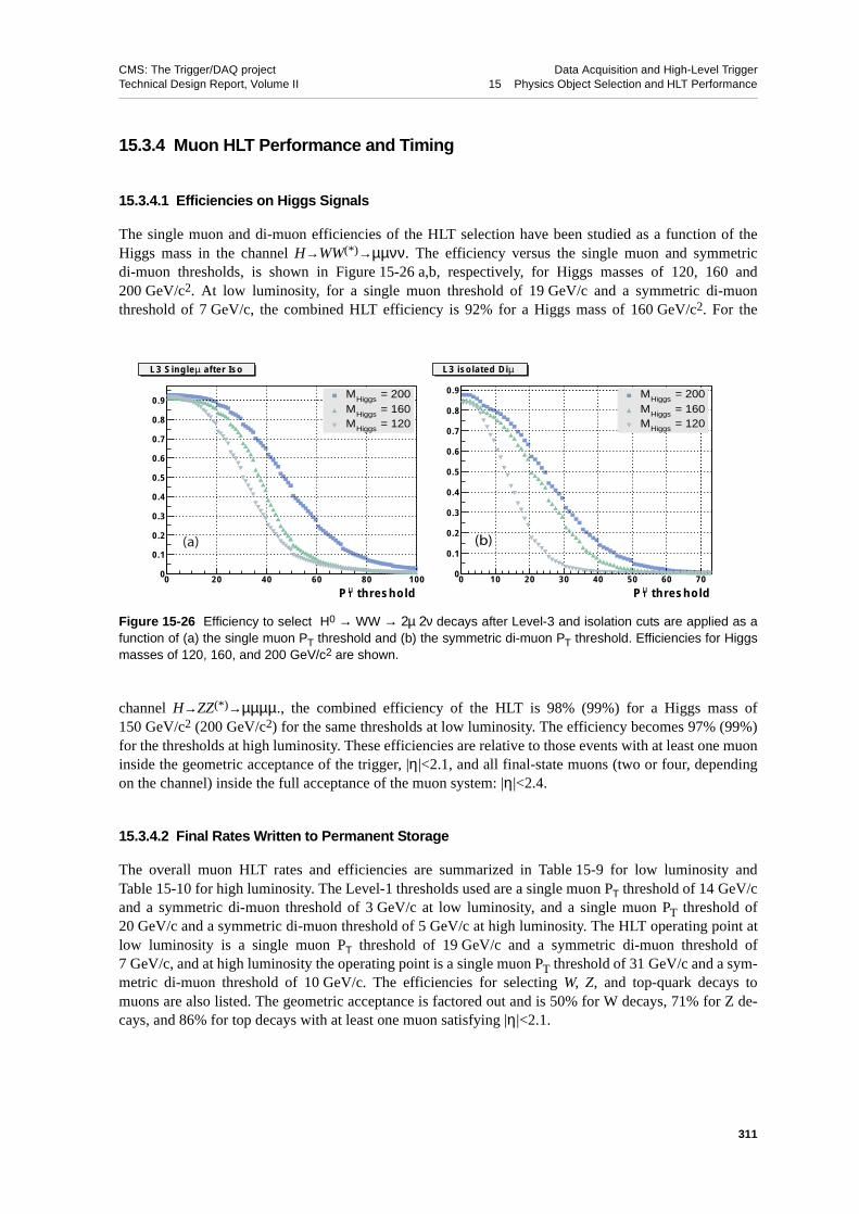
CMS: The Trigger/DAQ project Data Acquisition and High-Level TriggerTechnical Design Report, Volume II 15 Physics Object Selection and HLT Performance
15.3.4 Muon HLT Performance and Timing
15.3.4.1 Efficiencies on Higgs Signals
The single muon and di-muon efficiencies of the HLT selection have been studied as a function of theHiggs mass in the channel H→WW(*)→µµνν. The efficiency versus the single muon and symmetricdi-muon thresholds, is shown in Figure 15-26 a,b, respectively, for Higgs masses of 120, 160 and200 GeV/c2. At low luminosity, for a single muon threshold of 19 GeV/c and a symmetric di-muonthreshold of 7 GeV/c, the combined HLT efficiency is 92% for a Higgs mass of 160 GeV/c2. For the
channel H→ZZ(*)→µµµµ., the combined efficiency of the HLT is 98% (99%) for a Higgs mass of150 GeV/c2 (200 GeV/c2) for the same thresholds at low luminosity. The efficiency becomes 97% (99%)for the thresholds at high luminosity. These efficiencies are relative to those events with at least one muoninside the geometric acceptance of the trigger, |η|<2.1, and all final-state muons (two or four, dependingon the channel) inside the full acceptance of the muon system: |η|<2.4.
15.3.4.2 Final Rates Written to Permanent Storage
The overall muon HLT rates and efficiencies are summarized in Table 15-9 for low luminosity andTable 15-10 for high luminosity. The Level-1 thresholds used are a single muon PT threshold of 14 GeV/cand a symmetric di-muon threshold of 3 GeV/c at low luminosity, and a single muon PT threshold of20 GeV/c and a symmetric di-muon threshold of 5 GeV/c at high luminosity. The HLT operating point atlow luminosity is a single muon PT threshold of 19 GeV/c and a symmetric di-muon threshold of7 GeV/c, and at high luminosity the operating point is a single muon PT threshold of 31 GeV/c and a sym-metric di-muon threshold of 10 GeV/c. The efficiencies for selecting W, Z, and top-quark decays tomuons are also listed. The geometric acceptance is factored out and is 50% for W decays, 71% for Z de-cays, and 86% for top decays with at least one muon satisfying |η|<2.1.
Figure 15-26 Efficiency to select H0 → WW → 2µ 2ν decays after Level-3 and isolation cuts are applied as afunction of (a) the single muon PT threshold and (b) the symmetric di-muon PT threshold. Efficiencies for Higgsmasses of 120, 160, and 200 GeV/c2 are shown.
thresholdTµP
0 20 40 60 80 1000
0.1
0.2
0.3
0.4
0.5
0.6
0.7
0.8
0.9 = 200HiggsM = 160HiggsM = 120HiggsM
after IsoµL3 Single
thresholdTµP
0 10 20 30 40 50 60 700
0.1
0.2
0.3
0.4
0.5
0.6
0.7
0.8
0.9 = 200HiggsM = 160HiggsM = 120HiggsM
µL3 isolated Di
(a) (b)
311
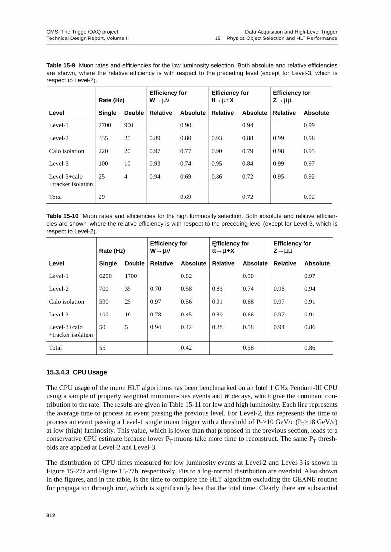
CMS: The Trigger/DAQ project Data Acquisition and High-Level TriggerTechnical Design Report, Volume II 15 Physics Object Selection and HLT Performance
15.3.4.3 CPU Usage
The CPU usage of the muon HLT algorithms has been benchmarked on an Intel 1 GHz Pentium-III CPUusing a sample of properly weighted minimum-bias events and W decays, which give the dominant con-tribution to the rate. The results are given in Table 15-11 for low and high luminosity. Each line representsthe average time to process an event passing the previous level. For Level-2, this represents the time toprocess an event passing a Level-1 single muon trigger with a threshold of PT>10 GeV/c (PT>18 GeV/c)at low (high) luminosity. This value, which is lower than that proposed in the previous section, leads to aconservative CPU estimate because lower PT muons take more time to reconstruct. The same PT thresh-olds are applied at Level-2 and Level-3.
The distribution of CPU times measured for low luminosity events at Level-2 and Level-3 is shown inFigure 15-27a and Figure 15-27b, respectively. Fits to a log-normal distribution are overlaid. Also shownin the figures, and in the table, is the time to complete the HLT algorithm excluding the GEANE routinefor propagation through iron, which is significantly less that the total time. Clearly there are substantial
Table 15-9 Muon rates and efficiencies for the low luminosity selection. Both absolute and relative efficienciesare shown, where the relative efficiency is with respect to the preceding level (except for Level-3, which isrespect to Level-2).
Rate (Hz)Efficiency for W→µν
Efficiency for tt→µ+X
Efficiency for Z→µµ
Level Single Double Relative Absolute Relative Absolute Relative Absolute
Level-1 2700 900 0.90 0.94 0.99
Level-2 335 25 0.89 0.80 0.93 0.88 0.99 0.98
Calo isolation 220 20 0.97 0.77 0.90 0.79 0.98 0.95
Level-3 100 10 0.93 0.74 0.95 0.84 0.99 0.97
Level-3+calo+tracker isolation
25 4 0.94 0.69 0.86 0.72 0.95 0.92
Total 29 0.69 0.72 0.92
Table 15-10 Muon rates and efficiencies for the high luminosity selection. Both absolute and relative efficien-cies are shown, where the relative efficiency is with respect to the preceding level (except for Level-3, which isrespect to Level-2).
Rate (Hz)Efficiency for W→µν
Efficiency for tt→µ+X
Efficiency for Z→µµ
Level Single Double Relative Absolute Relative Absolute Relative Absolute
Level-1 6200 1700 0.82 0.90 0.97
Level-2 700 35 0.70 0.58 0.83 0.74 0.96 0.94
Calo isolation 590 25 0.97 0.56 0.91 0.68 0.97 0.91
Level-3 100 10 0.78 0.45 0.89 0.66 0.97 0.91
Level-3+calo+tracker isolation
50 5 0.94 0.42 0.88 0.58 0.94 0.86
Total 55 0.42 0.58 0.86
312

CMS: The Trigger/DAQ project Data Acquisition and High-Level TriggerTechnical Design Report, Volume II 15 Physics Object Selection and HLT Performance
gains to be made by replacing GEANE with a faster method1. The total time listed in the last row repre-sents the average time spent per Level-1 event by the muon HLT algorithms, factoring in the rejectionpower at each level that reduces the rate to the next level. This time amounts to approximately 700 ms perL1A, including the time spent in GEANE.
Table 15-11 CPU usage of the muon HLT algorithms at low and high luminosity. The values given represent theaverage time to process an event passing the previous trigger level. Also listed is the time without the contribu-tion of the GEANE propagation routine.
Mean CPU Time (ms/event)L=2×1033cm-2s-1, PT>10 GeV/c
Mean CPU Time (ms/event)L=1034cm-2s-1, PT>18 GeV/c
HLT Algorithm Total Excluding GEANE Total Excluding GEANE
Level-2 640 100 580 100
Calorimeter isolation 100 25 90 40
Level-3 420 200 590 420
Pixel isolation 65 65 320 320
Tracker isolation 190 190 370 370
Total/L1 event 710 125 660 150
1. For calorimeter isolation (Section 15.3.2.1) GEANE is used for propagation to the ECAL/HCAL boundary.
Figure 15-27 Distribution of the CPU time spent for low luminosity events processed by (a) the muon Level-2and (b) the muon Level-3 algorithms on a 1 GHz Intel PIII processor. Also shown is time taken exclusive of theGEANE propagation routine.
T (s)0 0.5 1 1.5 2 2.5 3
0
200
400
600
800
1000
1200
1400 Excluding GEANETotal
Total L2 time
T (s)0 0.5 1 1.5 2 2.5 3
0
5
10
15
20
25
30 Excluding GEANETotal
Total L3 time
(a) (b)
313

CMS: The Trigger/DAQ project Data Acquisition and High-Level TriggerTechnical Design Report, Volume II 15 Physics Object Selection and HLT Performance
15.4 Jet and Neutrino Identification
15.4.1 Jet-finding Algorithm
Before jet-finding is executed in the HLT, the calorimeter data is organized into “towers" using the η−φsegmentation of the HCAL (0.087×0.087 in the barrel, near the edge of the endcap the η segmentation isas large as 0.175). There are 4176 such towers. In the ECAL barrel region, i.e. |η|<1.479, there are 25ECAL crystals per HCAL tower whereas in the endcap region, the number of crystals per tower varieswith η. The towers are treated as massless particles with energy equal to the scalar sum of the energies ofthe components of the tower, and using the center of the tower and z=0 for the nominal interaction pointto define the angles.
15.4.1.1 Basic Algorithm for Jet-finding
Global jet-finding is done using a simple iterative cone algorithm. In this algorithm, a list of towers ismade, and a “protojet” is formed using the direction of the tower from the list with the highest ET (the“seed tower”) as the protojet direction. The direction of the protojet is calculated from the transverse-en-ergy-weighted angles of the towers in a cone around the protojet direction in η-φ space, and the transverseenergy of the protojet is calculated using the direction of the protojet and the sum the energies of the tow-ers in the cone. The direction of the protojet is used to seed a new protojet. The procedure is repeated untilthe energy of the protojet changes by less than 1% between iterations and the direction of the protojetchanges in ∆η2+∆φ2 by less than 0.01, or until 100 iterations is reached. When a stable protojet is found,the towers in the stable jet are removed from the list of objects, and the procedure is repeated until no ob-jects are left in the list or until the tower with the highest ET is below a “seed” threshold, which is a pa-rameter of the algorithm. This simple iterative algorithm has no sophisticated splitting and mergingpresciption, and is therefore fast. Offline, a more complete algorithm, such as those suggested by the‘‘Run II Jet Algorthms Working Group” [15-11], will eventually be implemented. The offline algorithmwill also use more sophisticated algorithms that use more information than just the tower energies andgive improved energy resolution. There are currently promising results on energy flow algorithms andnew types of algorithms for the very high luminosity conditions at the LHC [15-12]. For the HLT, howev-er, a simple algorithm is clearly preferable.
Jet-finding is currently carried out using all calorimeter towers, instead of just those around Level-1 jetcandidates. However, different HLT triggers can require that the HLT jet candidates match to Level-1 can-didates to simplify trigger efficiency calculations.
15.4.1.2 Parameter Choice for Jet-finding Algorithm
The simple cone algorithm has three parameters, namely the size of the cone, the seed threshold, and theminimum jet ET. These parameters were optimized for high luminosity conditions. The resulting valuesare 0.5 (cone size), 2 GeV (seed threshold) and 10 GeV (jet threshold). Studies of different parameter set-tings for low luminosity are ongoing.
At the parton level, a jet has a reasonably narrow core in η−φ space that contains most of its energy.However, because of soft gluon emission, the cone size that gives the best energy resolution for the partoncan be quite large. When the jet is reconstructed in the calorimeter, however, a large cone will have a larg-er noise contribution, both from electronic noise and from energy from particles from pileup and from un-derlying event. Figure 15-28 displays the resolution at high luminosity for particle-level (“generator”) jets
314

CMS: The Trigger/DAQ project Data Acquisition and High-Level TriggerTechnical Design Report, Volume II 15 Physics Object Selection and HLT Performance
formed using a cone size of 0.7 when reconstructed in the calorimeter using a cone size of 0.5 and 0.7, forthe two regions |η|<1 and 3.5<|η|<4.5. The cone 0.5 has signficantly better resolution at high rapidity andlow ET. It has similar resolution everywhere else.
Figure 15-29 shows, for a high luminosity tt Monte Carlo sample, the invariant mass of the jets that bestmatch the generator level quarks from W decay for both cone 0.5 and cone 0.7 jets. The cone 0.5 jets givea slightly better resolution.
The seed thresholds cause an inefficiency for low ET jets that depends on the details of jet fragmentationand is therefore difficult to model. While modern offline jet finding algorithms may try to be seedless (see
Figure 15-28 Jet ET resolution as a function of generator jet ET, for two cone sizes (0.5 and 0.7) for jets with|η|<1 (left) and 3.5<|η|<4.5 (right). The resolution is defined as the R.M.S. of the difference between the ET of agenerator-level jet, found in a 0.7 cone, and the offline jet divided by the ET of the generator-level jet.
Figure 15-29 The reconstructed di-jet mass, at high luminosity, for the jets that most closely match the W decaypartons in tt events for two different cone sizes. The narrower distribution is for a cone size of 0.5 and thebroader for a cone size of 0.7.
ET (GeV)
0
0.05
0.1
0.15
0.2
0.25
0.3
0.35
0.4
0.45
0.5
0 20 40 60 80 100120140160180200
σ/E T
R=0.7
R=0.5
ET (GeV)
0
0.05
0.1
0.15
0.2
0.25
0.3
0.35
0.4
0.45
0.5
0 20 40 60 80 100120140160180200
R=0.7
R=0.5
σ/E T
R=0.5Mean=83..8σ=18.0
R=0.7Mean=92.4σ=22.5
di-jet mass (GeV/c2)0
200
400
600
800
1000
1200
0 50 100 150 200 250 300
315

CMS: The Trigger/DAQ project Data Acquisition and High-Level TriggerTechnical Design Report, Volume II 15 Physics Object Selection and HLT Performance
Reference [15-11]), at the trigger level a seed helps reduce the number of fake jets, which can otherwisebe created by noise and pileup and which typically have ET<50 GeV, and speeds up the time for jet find-ing. Figure 15-30 shows the rapidity distribution of reconstructed jets in a sample of Z′ events, withM(Z′)=120 GeV/c2, for two different seed thresholds. The left-hand plot, which shows the distribution fora 1 GeV seed, shows a significant excess of jets with low transverse energy with central rapidity. Thesefake jets are greatly reduced when a higher seed (3 GeV) is used, as shown in the right hand side ofFigure 15-30. Figure 15-31 shows the efficiency to reconstruct jets as a function of the ET of the jet fordifferent values of the seed threshold. Since none of the current triggers have jet thresholds below 30GeV, a 2 GeV seed is used.
A low minimum jet ET is needed for calibrating the jets for the Monte Carlo in order to avoid biases thatcome from the effects of noise and pileup, as described in the following section. The cut used in this anal-ysis is 10 GeV.
Figure 15-30 The distribution of η versus ET for jets in Monte Carlo simulation of the decay of a Z’ with mass120 GeV/c2. Left: a seed of 1 GeV is used; right: a seed of 3 GeV is used.
Figure 15-31 Efficiency to find an offline jet that matches a generator-level jet, as a function of the genera-tor-level jet ET at high luminosity.
20
40
60
80
100
120
140
-2.5 -2 -1.5 -1 -0.5 0 0.5 1 1.5 2 2.5
ENTRIES 32993
η jet
E T jet (
GeV
)
20
40
60
80
100
120
140
-2.5 -2 -1.5 -1 -0.5 0 0.5 1 1.5 2 2.5
ENTRIES 7659
η jet
E T jet (
GeV
)
0
0.2
0.4
0.6
0.8
1
1.2
1.4
20 25 30 35 40 45 50 55 60 65 70
ET genjet
(GeV)
jet-
genj
et m
atch
ing
effic
ienc
y
Z ′ (120) → jj
● Seed = 1.0 GeV■ Seed = 1.5 GeV▲ Seed = 2.0 GeV▼ Seed = 3.0 GeV
316

CMS: The Trigger/DAQ project Data Acquisition and High-Level TriggerTechnical Design Report, Volume II 15 Physics Object Selection and HLT Performance
15.4.1.3 Jet Energy Scale Corrections
The CMS calorimeter system is optimized for the precision measurement of electrons and photons, andhas a non-linear response to pions. Since the energy of a typical pion in a jet is roughly proportional to1/sin(θ), the response of the calorimeter to jets of a given transverse energy varies with η. In addition, be-cause only those channels that are above a threshold are read out (“one-sided zero-supression”), instead ofthose both above one threshold and below another (“two-sided zero-supression”), and which is set at avalue equal to ≈2σ of the noise pedestal in the HCAL and ECAL, a random cone on the calorimeter willhave a positive energy due to noise alone. Table 15-12 shows the size of the offset due to noise versus thesetting for the zero-supression threshold (in number of noise σ). A two-sided zero-supression threshold iscurrently under investigation. At high luminosity, there will be an additional offset due to energy fromparticles from pileup interactions.
Corrections for these effects are introduced both at Level-1 and in the HLT. At the start of the experiment,the corrections will be derived from Monte Carlo data by comparing the energies of jets found using thegenerator-level particles of the hard interaction (excluding particles from “pileup" interactions) to jetsfound in the calorimeter. As soon as sufficient data is collected, new corrections will be derived from sin-gle photon plus jets data and Z boson plus jet data.
For the purposes of this TDR, the Monte Carlo jets are calibrated so that the mean response for a genera-tor jet is equal to the generator jet energy. This technique is expected to yield results that are virtuallyidentical to those that would be obtained from a full calibration using events with photon and a jet.Figure 15-32 shows the size of the typical correction for HLT jets, obtained from simulation, for low lu-minosity and high luminosity running conditions. The correction can be as large as 20% for low-ET(40 GeV) jets.
The current correction is obtained by fitting the mean reconstructed ET, <ETrec>, as a function of the gen-
erator-level ET, ETgen, to a quadratic function: <ET
rec> = A(ETgen)2 + BET
gen + C where A, B and C arefunctions of η. The resolution of the ET measurement for jets before and after corrections, at both low andhigh luminosity, is shown in Figure 15-33 for cone 0.5 jets. The main effect of the corrections is the re-moval of the η dependence of the trigger efficiency, while the resolution is improved only slightly.
The resolution for high ET jets (ET>300 GeV) is similar at low and high luminosity, while the resolutionat lower ET values is significantly worse at high luminosity. As an example, the resolution for jets withET=40 GeV is approximately 19% at low luminosity and 24% at high luminosity. Work is ongoing in im-proving the jet energy resolution at high luminosity.
Table 15-12 Amount of energy in a cone of 0.5 due to noisealone for various values of a zero-supression threshold.
threshold (number of noise σ) energy in cone (GeV)
none 0.0
0 45.2
1 27.3
2 7.6
3 0.5
317

CMS: The Trigger/DAQ project Data Acquisition and High-Level TriggerTechnical Design Report, Volume II 15 Physics Object Selection and HLT Performance
15.4.1.4 Fake Jet Supression
At high luminosity, with a high number of interactions per crossing, low ET jets from the hard scatteringcan be mismeasured as high ET jets. This happens mainly when either particles or a small jet from one pi-leup interaction impact the calorimeter near one of the low ET jets creating a jet with higher ET, a “fakejet”. Fake jets can also be created when particles from different interactions impact near each other in thecalorimeter. In addition, the magnetic field sweeps charged particles with transverse momentum below0.77/c GeV out of the barrel and into the endcap region of the calorimeter. This sweeping effect prevents
Figure 15-32 Ratio of reconstructed to generated jet ET for HLT jets versus η and versus ET, before and afterjet energy scale corrections. Left: low luminosity; right: high luminosity.
Figure 15-33 Resolution for HLT jets before (triangles) and after (circles) jet energy scale calibration. Left: lowluminosity; right: high luminosity.
00.20.40.60.8
11.21.4
50 100 150 200 250 300 350 400Particle Jet Et (GeV)
Et C
AL
O J
ET/E
t PA
RT
JE
T
calibrated jetsraw jets
L=2x1033 cm-2s-1
Jets (R=0.5)
η
Et C
AL
O J
ET/E
t PA
RT
JE
T
calibrated jetsraw jets
L=2x1033 cm-2s-1
Jets (R=0.5)
00.20.40.60.8
11.21.4
0 0.5 1 1.5 2 2.5 3 3.5 4 4.5 5
00.20.40.60.8
11.21.4
50 100 150 200 250 300 350 400Particle Jet Et (GeV)
Et C
AL
O J
ET/E
t PA
RT
JE
T
calibrated jetsraw jets
L=1034 cm-2s-1
Jets (R=0.5)
η
Et C
AL
O J
ET/E
t PA
RT
JE
T
calibrated jetsraw jets
L=1034 cm-2s-1
Jets (R=0.5)
00.20.40.60.8
11.21.4
0 0.5 1 1.5 2 2.5 3 3.5 4 4.5 5
Particle Jet ET (GeV)
σ(ET)/ET = 1.18/√ET + 0.07
L = 2x1033cm-2s-1
Jets (R=0.5)
0
0.1
0.2
0.3
0.4
0.5
0.6
0 100 200 300 400 500 600 700
σ(ET)/ET = 1.48/√ET + 0.07
σ(E
T)/E
T
0
0.1
0.2
0.3
0.4
0.5
0.6
0 100 200 300 400 500 600 700Particle Jet ET (GeV)
σ(ET)/ET = 1.56/√ET + 0.05σ(ET)/ET = 1.85/√ET + 0.04
σ(E
T)/E
T
L = 1034cm-2s-1
Jets (R=0.5)
318

CMS: The Trigger/DAQ project Data Acquisition and High-Level TriggerTechnical Design Report, Volume II 15 Physics Object Selection and HLT Performance
more than half of the charged particles pointed toward the barrel from actually striking the calorimeter,severely altering the energy flow in the underlying and pileup events. The accidental overlap of these par-ticles with particles from the soft interactions causes the fake jet problem to be especially severe at theHE/HF boundary. Figure 15-34 shows the rapidity distribution of all calorimeter jets (solid) and the rapid-ity distribution of the subset of these that have a good match in η−φ to a jet made from generator-levelparticles from the hard scattering for jets with transverse energies above 20, 30, and 40 GeV. Above 40GeV, the number of fake jets is small.
Methods of supressing these fake jets at the trigger level have been studied using only calorimeter infor-mation for the HLT. Ongoing work is investigating the use of tracking (pixel) information for this pur-pose.
There is no unambiguous way to classify a jet as “fake” or “real”. Most jets found by the jet finder containsome particles from the hard scatter and some particles from the pile up events. The degree of “fakeness”that is acceptable will vary according to the particular trigger and physics channel. To measure the “real-ness” of a jet, the generator-level particles are extrapolated into the jet cone and the variable:
is defined. ET(vtxi) is the scalar sum of the ET’s of the particles extrapolating into the jet cone from the ith
vertex and ET(jet) is the ET of the jet. If a jet has more than a 50% of its ET contributed from a single ver-tex, i.e. R1>0.5, it is considered to be a real jet, otherwise it is considered to be a fake jet. Figure 15-35shows R1 versus ET and η for jets from an inclusive jet sample with 30<PT
hard<50 GeV, where PThard is
the transverse momentum transferred in the hard scattering subprocess at the parton level. Fake jets,which have low values for R1, tend to have low ET. In η, fake jets tend to be near the HE/HF boundary.
Fake jets should have a broader transverse distribution than real jets. To study this, two variables, S1 andS2 are introduced. S1 is the ET-weighted mean radius: , whereas S2 is the fractionof the ET in a cone of 0.25, . Only results from S2 are shown here, since bothvariables give similar results. Figure 15-36 shows the correlation between R1 and S2, showing that “fake”jets tend to have a large S2. An interesting variable is the fraction of jets with R1<0.5 that are rejectedversus those with R>0.5 that are kept, as a function of a cut on S2. Figure 15-37 shows the result, showingit is possible to keep real jets with a reasonable efficiency while supressing fake jets. For example, for an80% efficiency for selecting real jets, about half of the fake jets are rejected. However, this cut is not usedin the subsequent rate plots because it does not seem necessary in order to achieve the desired rate to tape,and it is clearly preferable not to bias the jet samples with these cuts if possible. These parameters shouldbe useful in the development of more sophisticated triggers in the future.
Figure 15-34 η distribution of reconstructed jets for three thresholds on the jet ET. Solid line: all reconstructedjets. Dashed line: only jets with a good match to a generator-level jet from the hard scattering.
η(jet)
ET>20GeV
#jet
s/0.
2
ET>30GeV ET>40GeV
-4 -3 -2 -1 0 1 2 3 4η(jet)η(jet)
-4 -3 -2 -1 0 1 2 3 4 -4 -3 -2 -1 0 1 2 3 4
R1 maxET vtxi( )ET jet )( )--------------------
=
S1 ETr∑( ) ET∑( )⁄=S2 ET 0.25( )( ) ET 0.5( )( )⁄=
319

CMS: The Trigger/DAQ project Data Acquisition and High-Level TriggerTechnical Design Report, Volume II 15 Physics Object Selection and HLT Performance
15.4.1.5 Jet Rates
The jet rates are insensitive to the details of the simulation and are robust against reasonable changes injet algorithms. For example, Figure 15-38 shows the rates at low and high luminosity for a 1 jet trigger forjets reconstructred at the generator level using particles from only the hard scattering (labeled in the Fig-ure as Signal GenJet) and using generator-level particles from all interactions (labeled in the Figure asin-time GenJet). The Figure also shows the HLT jet rates both before and after jet energy scale correc-
Figure 15-35 R1, a measure of the realness of a jet, versus the ET and η of the jet. Top: scatter plot of R1 vs ET(left) and η (right). Bottom: mean R1 vs ET (left) and η (right). R1 is small when the jet has sizable contributionsfrom more than one vertex.
Figure 15-36 Fraction of jet ET in a cone of radius0.25 versus R1, the measure of fakeness of a jet. Asmall value of R1 means the jet has non-negligiblecontributions from more than one primary vertex.
Figure 15-37 Efficiency versus rejection for a cut onthe fraction of the jet ET in a cone of 0.25 for removingfake jets.
1.4
1.2
1.0
0.8
0.6
0.4
0.2
25 30 35 40 45 50 55
1.0
0.8
0.6
0.4
0.2
25 30 35 40 45 50 55
Reconstructed jets, jet ET>20 GeV, seed ET>2 GeV
E T fra
ctio
n in
con
e R
=0.2
5
320

CMS: The Trigger/DAQ project Data Acquisition and High-Level TriggerTechnical Design Report, Volume II 15 Physics Object Selection and HLT Performance
tions. The rates for all these different types of jets are basically the same. At fixed ET, the high luminosityrates are about five times larger than the rates at low luminosity, as expected.
Figure 15-39 shows the rate for single-jet, 3-jet, and 4-jet triggers at low and high luminosity. The x-axisis the threshold on the calibrated jet ET for the HLT rate curve. Figure 15-40 shows the single-jet rate andthe incremental rate from 2-jet and 3-jet triggers rates.
The effect of different algorithms and different detectors can be studied by comparing the rate as a func-tion of the generator-level jet ET. The latter is approximated by the cut on the offline jet ET that gives 95%efficiency for the generator-level jet ET. The relationship between the value of the cut and the genera-tor-level jet ET is linear, and is given by
• for HLT jets at low luminosity;
• for HLT jets at high luminosity;
• for Level-1 jets at low luminosity;
• for Level-1 jets at high luminosity;
Figure 15-39 and Table 15-13 show the results.
The thresholds for triggers that use only jets are very high. Most HLT triggers on physics channels withjets will need something besides jets in the trigger to have an acceptable rate and an acceptably lowthreshold on jet ET. As shown in the sections on SUSY (15.8.3.2) and the invisible Higgs (15.8.3.3), it isusually not difficult to find something else in the event to use as part of the trigger.
Figure 15-38 Rates for a single- jet trigger at the generator-level using only particles from the hard scattering tomake the jets and also using all particles, including those from the pileup interactions, at both low and high lumi-nosity. Also shown are the HLT single-jet trigger rates both before and after jet energy scale corrections at lowand high luminosity. The open (filled) symbols show the low (high) luminosity rate.
10-2
10-1
1
10
10 2
10 3
10 4
10 5
10 6
10 7
0 200 400 600 800 1000
● In-time GenJet
■ HLT corrected
★ HLT uncorrected
▲ Signal Genjet
Single Jet ET Cutoff [GeV]
Rat
e [H
z]
ET gen( ) 1.13ET cut( ) 11.1GeV+=
ET gen( ) 1.12ET cut( ) 17.4GeV+=
ET gen( ) 1.18ET cut( ) 17.2GeV+=
ET gen( ) 1.17ET cut( ) 19.8GeV+=
321

CMS: The Trigger/DAQ project Data Acquisition and High-Level TriggerTechnical Design Report, Volume II 15 Physics Object Selection and HLT Performance
Figure 15-39 Rates for 1, 3, and 4-jet triggers as a function of calibrated jet ET (x axis). Also shown is the ratefor the cut that gives 95% efficiency for the generator-ET shown on the x-axis are given. Left: low luminosity.Right: high luminosity.
Figure 15-40 The rates for 1-jet events, and the incremental 2-jet and 3-jet rates, given a 1-jet threshold of350 GeV, at low luminosity (left), and a 1-jet threshold of 650 GeV at high luminosity (right).
Table 15-13 Jet rate summary table. The table gives the generator-level jet ET where the cut (in GeV)on the reconstructed jet ET gives 95% efficiency for this generator-level jet ET and also gives by itself arate of 1 kHz (Level-1) and 1 Hz (HLT). The actual value of the cut on ET that corresponds to the 95%efficiency points is given in parentheses.
1-jet trigger 2-jet trigger 3-jet trigger 4-jet trigger
low luminosity Level-1 177 (135) 140 (104) 85 (57) 70 (45)
high luminosity Level-1 248 (195) 199 (153) 112 (79) 95 (64)
low luminosity HLT 657 (571) 564 (489) 247 (209) 149 (122)
high luminosity HLT 860 (752) 748 (652) 326 (275) 199 (162)
L = 2x1033cm-2s-1
Jets (R=0.5)
Calibrated Single JetSingle Jet, 95%EffCalibrated Triple JetTriple Jet, 95% EffCalibrated Quad JetQuad Jet, 95% Eff
ET[GeV]
Rat
e [H
z]
10-2
10-1
1
10
10 2
10 3
10 4
10 5
10 6
10 7
0 200 400 600 800
Calibrated Single JetSingle Jet, 95%EffCalibrated Triple JetTriple Jet, 95% EffCalibrated Quad JetQuad Jet, 95% Eff
Calibrated Single JetSingle Jet, 95%EffCalibrated Triple JetTriple Jet, 95% EffCalibrated Quad JetQuad Jet, 95% Eff
10-2
10-1
1
10
10 2
10 3
10 4
10 5
10 6
10 7
0 200 400 600 800
Calibrated Single JetSingle Jet, 95%EffCalibrated Triple JetTriple Jet, 95% EffCalibrated Quad JetQuad Jet, 95% Eff
L = 1034cm-2s-1
Jets (R=0.5)
ET[GeV]R
ate
[Hz]
(GeV)cuttE
0 100 200 300 400 500 600 700 800
Inte
gra
ted
Rate
(H
z)
10-2
10-1
1
10
102
103
104
105
106
107
1 Jet Inclusive Rate
2-Jet Additional Rate for 1-jet cut = 350 GeV
3-Jet Additional Rate for 2-jet cut = 300 GeV
(GeV)cuttE
0 100 200 300 400 500 600 700 800
Inte
gra
ted
Rate
(H
z)
10-2
10-1
1
10
102
103
104
105
106
107 1 Jet Inclusive Rate
2-Jet Additional Rate for 1-jet cut = 650 GeV
3-Jet Additional Rate for 2-jet cut = 300 GeV
3-Jet Additional Rate for 2-jet cut = 400 GeV
3-Jet Additional Rate for 2-jet cut = 500 GeV
322
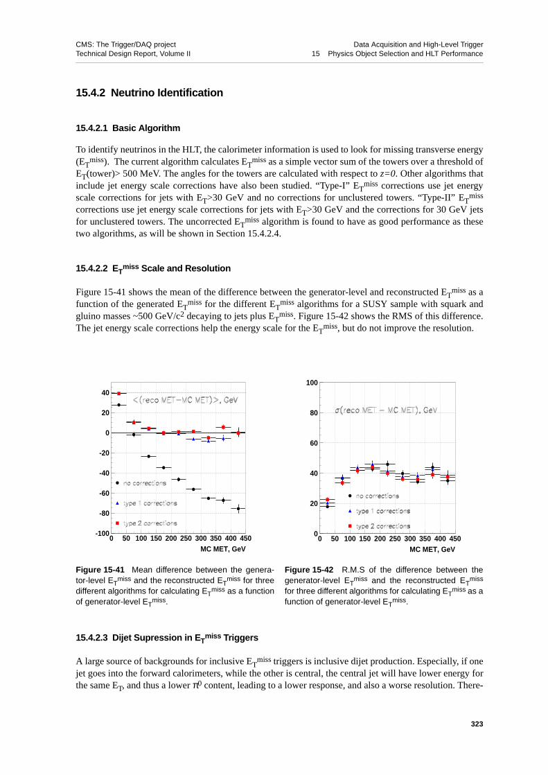
CMS: The Trigger/DAQ project Data Acquisition and High-Level TriggerTechnical Design Report, Volume II 15 Physics Object Selection and HLT Performance
15.4.2 Neutrino Identification
15.4.2.1 Basic Algorithm
To identify neutrinos in the HLT, the calorimeter information is used to look for missing transverse energy(ET
miss). The current algorithm calculates ETmiss as a simple vector sum of the towers over a threshold of
ET(tower)> 500 MeV. The angles for the towers are calculated with respect to z=0. Other algorithms thatinclude jet energy scale corrections have also been studied. “Type-I” ET
miss corrections use jet energyscale corrections for jets with ET>30 GeV and no corrections for unclustered towers. “Type-II” ET
miss
corrections use jet energy scale corrections for jets with ET>30 GeV and the corrections for 30 GeV jetsfor unclustered towers. The uncorrected ET
miss algorithm is found to have as good performance as thesetwo algorithms, as will be shown in Section 15.4.2.4.
15.4.2.2 ETmiss Scale and Resolution
Figure 15-41 shows the mean of the difference between the generator-level and reconstructed ETmiss as a
function of the generated ETmiss for the different ET
miss algorithms for a SUSY sample with squark andgluino masses ~500 GeV/c2 decaying to jets plus ET
miss. Figure 15-42 shows the RMS of this difference.The jet energy scale corrections help the energy scale for the ET
miss, but do not improve the resolution.
15.4.2.3 Dijet Supression in ETmiss Triggers
A large source of backgrounds for inclusive ETmiss triggers is inclusive dijet production. Especially, if one
jet goes into the forward calorimeters, while the other is central, the central jet will have lower energy forthe same ET, and thus a lower π0 content, leading to a lower response, and also a worse resolution. There-
Figure 15-41 Mean difference between the genera-tor-level ET
miss and the reconstructed ETmiss for three
different algorithms for calculating ETmiss as a function
of generator-level ETmiss.
Figure 15-42 R.M.S of the difference between thegenerator-level ET
miss and the reconstructed ETmiss
for three different algorithms for calculating ETmiss as a
function of generator-level ETmiss.
-100
-80
-60
-40
-20
0
20
40
0 50 100 150 200 250 300 350 400 450MC MET, GeV
0
20
40
60
80
100
0 50 100 150 200 250 300 350 400 450MC MET, GeV
323

CMS: The Trigger/DAQ project Data Acquisition and High-Level TriggerTechnical Design Report, Volume II 15 Physics Object Selection and HLT Performance
fore, the ETmiss will tend to be along the direction of the central jet. Several ways to help remove this kind
of background have been considered: a cut on the opening angle in φ, ∆φ, between the ETmiss and the
leading jet, between the ETmiss and the jet with the second highest ET, on the opening angle between the
leading and second jet, the opening angle between the leading jet and the sum of the second and third jet,and the opening angle between the ET
miss and the sum of the second and third jet. Figures 15-43 and15-44 show the distributions for these variables for inclusive dijet events with 80<PT
hard<120 GeV. Thevariables that correlate the direction of the ET
miss with the jet directions turn out to be inefficient forSUSY type events (see Section 15.8.3.2, "Supersymmetry Searches"). The best variable seems to be theopening angle between the leading and second jet. However, this cut is only effective for very high valuesof ET
miss. Current plans for the HLT selection do not include a cut of this type.
15.4.2.4 ETmiss Rates
Figure 15-45 shows the ETmiss rates at the generator level at both low and high luminosity. At the genera-
tor-level the ETmiss is due to neutrinos produced in the decays of heavy flavors and due to particles which
have |η|>5.0 and are therefore outside of the coverage of the calorimeter. In general, most of the rate be-low 60 GeV is due to the finite coverage of the calorimeter, while above 60 GeV the rate is dominated byheavy flavor production. The effect of the finite coverage of the calorimeter is more pronounced at highluminosity. Figure 15-45 also shows the Level-1 and HLT ET
miss rates at low and high luminosity. Thereare currently no plans for triggers demanding only ET
miss and no other physics object, e.g. a jet, at theHLT. Triggers using jets and ET
miss are discussed in the section on physics selection. The above rates areshown for illustrative purposes only. The HLT rates are much larger than the generator-level rates, and are
Figure 15-43 Upper plot: Opening angle in φ betweenthe ET
miss and the direction of the sum of the secondand third jets with the highest ET. Lower plot: the open-ing angle in φ, between the ET
miss and the secondhighest ET jet. The plot contains inclusive dijets with80 < PT
hard < 120 GeV/c and ETmiss > 50 GeV.
Figure 15-44 Upper plot: Opening angle in φ betweenthe direction of the highest ET jet and the direction ofthe sum of the second and third highest ET jets. Lowerplot: and the opening angle in φ, between the highestET jet and the second highest ET jet minus π. The plotcontains inclusive dijets with 80 < PT
hard < 120 GeV/cand ET
miss > 50 GeV.
324

CMS: The Trigger/DAQ project Data Acquisition and High-Level TriggerTechnical Design Report, Volume II 15 Physics Object Selection and HLT Performance
very sensitive to the details of the simulation. The non-smoothness of the rates is due to insufficient statis-tics in the lower bins in PT
hard.
Figure 15-46 shows the effect of requiring the opening angle in φ between the two leading jets be largerthan 0.5. This cut is only effective for large values of ET
miss. Figure 15-47 shows the rates when a jet withET above a threshold is also required as part of the trigger.
To faciliate comparisons between different algorithms and different experiments, it is convenient to plotthe rates as a function of the cut that gives 95% efficiency for a given generator-level ET
miss. Since inclu-sive dijet events have very little generator-level ET
miss, we use a signal sample to make a mapping be-
Figure 15-45 Generator-level ETmiss rates at low and
high luminosity. Also shown are the HLT ETmiss rates
at low and high luminosity.
Figure 15-46 HLT ETmiss rates at low and high lumi-
nosity before and after requiring the two leading jets tonot be back-to-back in φ within 0.5 radians.
Figure 15-47 Event rates as function of ETmiss when requiring a jet above various thresholds. Left: low luminos-
ity; right: high luminosity.
325
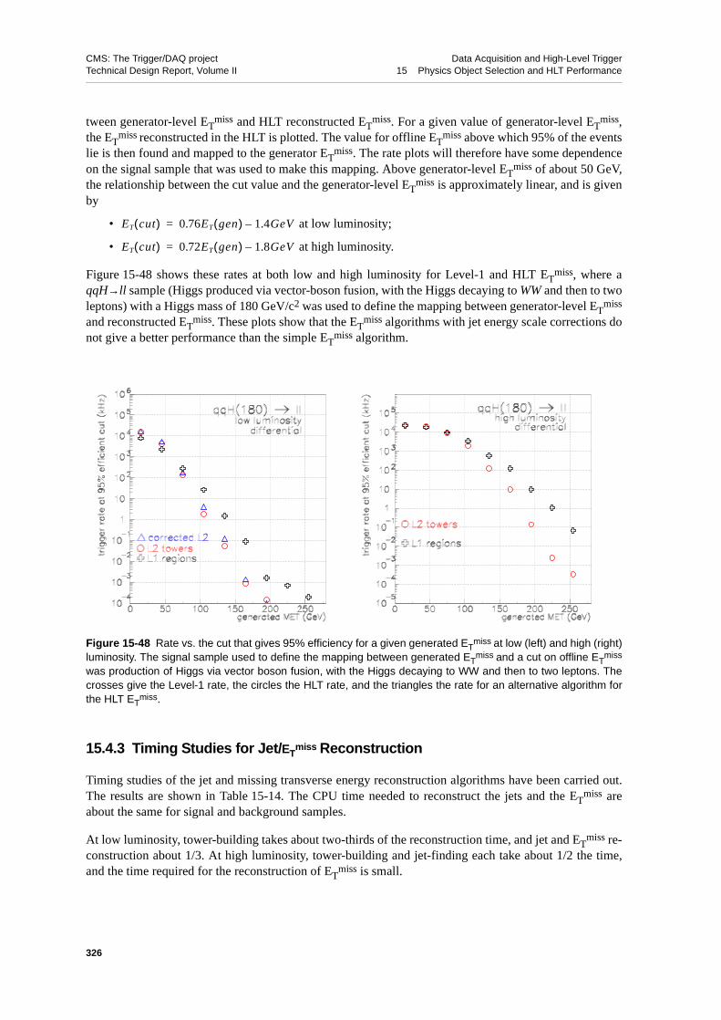
CMS: The Trigger/DAQ project Data Acquisition and High-Level TriggerTechnical Design Report, Volume II 15 Physics Object Selection and HLT Performance
tween generator-level ETmiss and HLT reconstructed ET
miss. For a given value of generator-level ETmiss,
the ETmiss reconstructed in the HLT is plotted. The value for offline ET
miss above which 95% of the eventslie is then found and mapped to the generator ET
miss. The rate plots will therefore have some dependenceon the signal sample that was used to make this mapping. Above generator-level ET
miss of about 50 GeV,the relationship between the cut value and the generator-level ET
miss is approximately linear, and is givenby
• at low luminosity;
• at high luminosity.
Figure 15-48 shows these rates at both low and high luminosity for Level-1 and HLT ETmiss, where a
qqH→ll sample (Higgs produced via vector-boson fusion, with the Higgs decaying to WW and then to twoleptons) with a Higgs mass of 180 GeV/c2 was used to define the mapping between generator-level ET
miss
and reconstructed ETmiss. These plots show that the ET
miss algorithms with jet energy scale corrections donot give a better performance than the simple ET
miss algorithm.
15.4.3 Timing Studies for Jet/ETmiss Reconstruction
Timing studies of the jet and missing transverse energy reconstruction algorithms have been carried out.The results are shown in Table 15-14. The CPU time needed to reconstruct the jets and the ET
miss areabout the same for signal and background samples.
At low luminosity, tower-building takes about two-thirds of the reconstruction time, and jet and ETmiss re-
construction about 1/3. At high luminosity, tower-building and jet-finding each take about 1/2 the time,and the time required for the reconstruction of ET
miss is small.
Figure 15-48 Rate vs. the cut that gives 95% efficiency for a given generated ETmiss at low (left) and high (right)
luminosity. The signal sample used to define the mapping between generated ETmiss and a cut on offline ET
miss
was production of Higgs via vector boson fusion, with the Higgs decaying to WW and then to two leptons. Thecrosses give the Level-1 rate, the circles the HLT rate, and the triangles the rate for an alternative algorithm forthe HLT ET
miss.
ET cut( ) 0.76ET gen( ) 1.4GeV–=
ET cut( ) 0.72ET gen( ) 1.8GeV–=
326

CMS: The Trigger/DAQ project Data Acquisition and High-Level TriggerTechnical Design Report, Volume II 15 Physics Object Selection and HLT Performance
Table 15-14 CPU requirements for Jet and ETmiss reconstruction in the HLT. Times are in ms for a Pentium-III,
1 GHz CPU.
A0/H0→ττ events, MH=500 GeV/c2
inclusive dijets with 50<PT
hard<80 GeV
Low lum High Lum Low Lum High Lum
tower-building 26 38 24 36
Jet reconstruction 9 34 9 45
ETmiss calculation 5 7 5 7
Total jet/ETmiss reconstruction 14 42 14 43
327

CMS: The Trigger/DAQ project Data Acquisition and High-Level TriggerTechnical Design Report, Volume II 15 Physics Object Selection and HLT Performance
15.5 τ-lepton Identification
The High-Level Trigger algorithms for τ identification are designed to be used in the selection of isolatedτ leptons such as those expected in the MSSM Higgs decays A0/H0→ττ and H+→τν. The final-state sig-natures involve events with a lepton plus a τ-jet, two τ-jets or only one τ-jet. The algorithms are studied atboth low and high luminosities, and for the low luminosity case two detector configurations are consid-ered, a full pixel system and the possible staged pixel system (Section 14.2.1). The evaluation of the algo-rithm performance consists of measuring the selection efficiencies of the benchmark signal samplesA0/H0→ττ and H+→τν and the corresponding efficiency of the QCD di-jet background. An important el-ement of the analysis, like all other HLT analyses, is the minimization of the CPU time required for theselection. Both signal and QCD di-jet background samples are required to pass the Level-1 Trigger selec-tions described in Section 15.1.3, "Level-1 Trigger Settings and Rates".
The QCD two-jet events were generated with PYTHIA in several different bins of PThard. Most of the
contribution to the Level-1 τ-trigger rate (~85−95%) comes from three bins: 50 < PThard <80 GeV/c,
80 < PThard < 120 GeV/c and 120 < PT
hard < 170 GeV/c. These bins were used to evaluate the rejectionfactor of the HLT against the QCD background. Signal events were selected at the generator level withloose offline analysis requirements on leptons (e and µ) and τ-jets [15-13], [15-14] and [15-15]:
1. for A0/H0→2τ→l + τ-jet: PTl > 14 GeV/c, PT
τ-jet > 30 GeV/c, |ηl, τ-jet| < 2.4;
2. for A0/H0→2τ→2τ-jet: PTτ-jet > 45 GeV/c, |ητ-jet| < 2.4;
3. for H+→τν→τ-jet: PTτ-jet > 80 GeV/c, |ητ-jet| < 2.4.
The following definitions are used in the rest of the current section:
• first (second) “Level-1 τ-jet” is the first (second) jet from the τ-jet list provided by the Global Cal-orimeter trigger. Jets in this list are ordered in ET (the first jet has the highest ET).
• first (second) “Calo jet” is a jet reconstructed with the calorimeter in a region centred on the first(second) Level-1 τ-jet.
As in the previous sections, the nominal pixel detector configuration with three barrel layers and two for-ward disks is referred to as the “full” pixel detector whereas the start-up detector with only two barrel lay-ers and one forward disk is referred to as the “staged” pixel detector configuration.
The identification of τ-jets involves information from both the calorimeter and tracking detectors. Thefollowing sections describes the details.
15.5.1 Calorimeter-based τ Selection.
The τ lepton decays hadronically 65% of the time, producing a “τ-jet”, which is a jet-like cluster in thecalorimeter containing a relatively small number of charged and neutral hadrons. When the PT of the τ-jetis large compared to the τ mass, these hadrons have relatively small momentum in the plane transverse tothe τ-jet axis. In 77% of hadronic τ decays, the τ-jet consists of only one charged hadron and a number ofπ0s (“one prong” decays). Because of these features hadronic τ decays produce narrow jets in the calorim-eter. About 90% of the τ-jet energy is contained in a very small cone of radius 0.15 to 0.20 and about 98%in a cone of 0.4 for τ-jets with ET > 50 GeV.
In the selection, isolation in the electromagnetic calorimeter is used. The parameter Pisol is defined as:
328

CMS: The Trigger/DAQ project Data Acquisition and High-Level TriggerTechnical Design Report, Volume II 15 Physics Object Selection and HLT Performance
where the sums run over transverse energy deposits in the electromagnetic calorimeter, and ∆R is the dis-tance in η-ϕ space from the τ-jet axis.
The identification of τ-jets begins with the reconstruction of a jet in a region centered on the Level-1 τ-jet.The Iterative Cone algorithm [15-16] with a cone size of 0.6 is used. The algorithm uses as input only thecalorimeter towers located within a cone of radius 0.8 around the Level-1 τ-jet direction. Restricting thenumber of towers considered by the jet finder results in a considerable speed-up of the jet finding process.For each jet found, the electromagnetic isolation parameter Pisol is calculated. Jets with Pisol < Pisol
cut areconsidered as τ candidates.
The identification of a τ-jet with the calorimeter will be referred to as the “Calorimeter Tau Trigger”. Theefficiency of the Calorimeter Tau Trigger for A0/H0→2τ→2τ-jet and QCD di-jet background events whenthe value of Pisol
cut is varied is shown in Figure 15-49 for both low and high luminosities when calorime-ter τ identification is applied to the first calorimeter jet.
The efficiency of the Higgs selection is essentially independent of the Higgs mass. Details of the Calorim-eter Tau Trigger optimization can be found in [15-17]. The entire selection procedure is very fast, as can
Figure 15-49 Efficiency of the Calorimeter Tau Trigger when applied to the first calorimeter jet inA0/H0 → 2τ → 2τ-jet and QCD di-jet events. MH = 200 and 500 GeV/c2 for low (left) and high (right) luminosity.
Table 15-15 CPU time, in ms of a 1 GHz CPU, for τ-jet identification with the calorimeter for QCD di-jet events.
Reconstruction step / luminosity 2×1033 cm-2s-1 1034 cm-2s-1
Build calorimeter towers 24 39
Regional finding of calo jets and Pisol calculation 9 15
Total time 33 54
Pisol ET
∆R 0.4<
∑ ET
∆R 0.13<
∑–=
0.4
0.5
0.6
0.7
0.8
0.9
1
1.1
1.2
0 0.1 0.2 0.3 0.4 0.5 0.6 0.7 0.8 0.9 1
ε(QCD bkg 50-170 GeV)
ε(H
(200
, 500
GeV
)→ττ
, τ→
1,3h
+X
)
L=2x1033cm-2s-1
Calo Tau Trigger on first Calo jet
MH=200 GeV
MH=500 GeV
0.4
0.5
0.6
0.7
0.8
0.9
1
1.1
1.2
0 0.1 0.2 0.3 0.4 0.5 0.6 0.7 0.8 0.9 1
ε(QCD bkg 50-170 GeV)
ε(H
(200,5
00 G
eV
)→ττ
, τ→
1,3
h+
X)
L=1034cm-2s-1
Calo Tau Trigger on first Calo jet
MH=200 GeV
MH=500 GeV
329
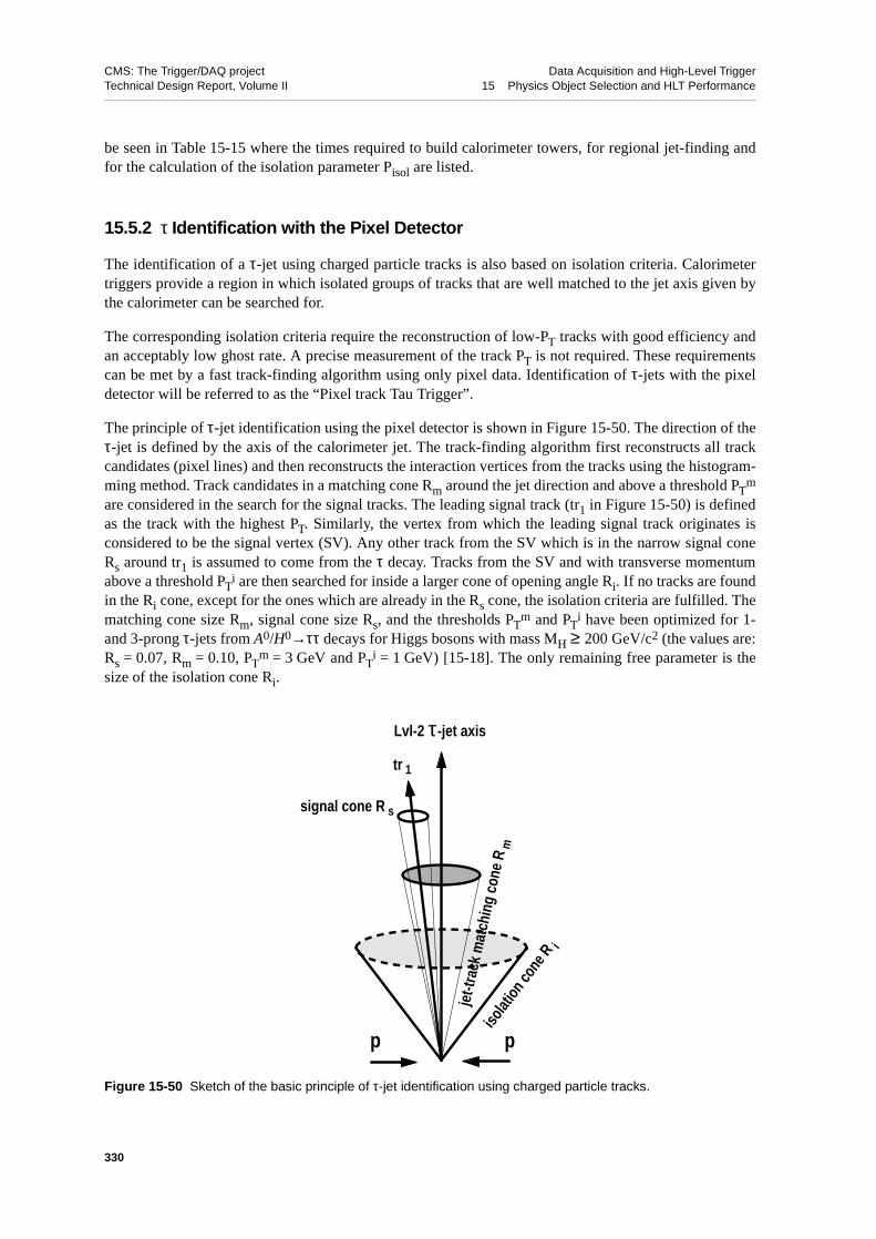
CMS: The Trigger/DAQ project Data Acquisition and High-Level TriggerTechnical Design Report, Volume II 15 Physics Object Selection and HLT Performance
be seen in Table 15-15 where the times required to build calorimeter towers, for regional jet-finding andfor the calculation of the isolation parameter Pisol are listed.
15.5.2 τ Identification with the Pixel Detector
The identification of a τ-jet using charged particle tracks is also based on isolation criteria. Calorimetertriggers provide a region in which isolated groups of tracks that are well matched to the jet axis given bythe calorimeter can be searched for.
The corresponding isolation criteria require the reconstruction of low-PT tracks with good efficiency andan acceptably low ghost rate. A precise measurement of the track PT is not required. These requirementscan be met by a fast track-finding algorithm using only pixel data. Identification of τ-jets with the pixeldetector will be referred to as the “Pixel track Tau Trigger”.
The principle of τ-jet identification using the pixel detector is shown in Figure 15-50. The direction of theτ-jet is defined by the axis of the calorimeter jet. The track-finding algorithm first reconstructs all trackcandidates (pixel lines) and then reconstructs the interaction vertices from the tracks using the histogram-ming method. Track candidates in a matching cone Rm around the jet direction and above a threshold PT
m
are considered in the search for the signal tracks. The leading signal track (tr1 in Figure 15-50) is definedas the track with the highest PT. Similarly, the vertex from which the leading signal track originates isconsidered to be the signal vertex (SV). Any other track from the SV which is in the narrow signal coneRs around tr1 is assumed to come from the τ decay. Tracks from the SV and with transverse momentumabove a threshold PT
i are then searched for inside a larger cone of opening angle Ri. If no tracks are foundin the Ri cone, except for the ones which are already in the Rs cone, the isolation criteria are fulfilled. Thematching cone size Rm, signal cone size Rs, and the thresholds PT
m and PTi have been optimized for 1-
and 3-prong τ-jets from A0/H0→ττ decays for Higgs bosons with mass MH ≥ 200 GeV/c2 (the values are:Rs = 0.07, Rm = 0.10, PT
m = 3 GeV and PTi = 1 GeV) [15-18]. The only remaining free parameter is the
size of the isolation cone Ri.
Figure 15-50 Sketch of the basic principle of τ-jet identification using charged particle tracks.
isolat
ion co
ne R i
jet-t
rack
mat
chin
g co
ne R
m
signal cone R s
Lvl-2 τ-jet axis
tr 1
p p
330

CMS: The Trigger/DAQ project Data Acquisition and High-Level TriggerTechnical Design Report, Volume II 15 Physics Object Selection and HLT Performance
The efficiency of the Pixel track Tau Trigger, at both low and high luminosity is shown in Figure 15-51when the size of the isolation cone is varied in the range 0.20-0.50. Pixel τ identification has been appliedfor the first calorimeter jet in A0/H0→2τ→2τ-jet and QCD di-jet events. The degradation of the perform-ance at high luminosity with respect to low luminosity is due to the larger readout inefficiency of the pixeldetector at high luminosity as well as the contamination of charged-particle tracks from pile-up in the iso-lation cone. The selection is essentially independent of the Higgs mass. Comparison between the full andstaged pixel systems shows that, at constant QCD background rate, the signal efficiency is degraded byapproximately 10% in the staged scenario.
The timing performance of the Pixel track Tau Trigger algorithm is shown in Table 15-16. It includes thetime to reconstruct clusters from the pixel digitized data and the time for reconstruction of the pixel linesand vertices. The time used by the isolation algorithm itself is negligible.
15.5.3 τ Identification Using Regional Track Finding
In this section an algorithm to select τ-jets using information from reconstructed tracks is described. Thisselection will be referred to as the “Track Tau Trigger”. The Track Tau Trigger performs the reconstruc-tion of only those tracks in restricted regions of interest (“regional tracking”), defined by the cones around
Figure 15-51 Efficiency of Pixel track Tau Trigger for the first calorimeter jet in A0/H0 → 2τ → 2τ - jet, for twoHiggs masses, MH = 200 and 500 GeV/c2, versus the efficiency for QCD di-jet background events. Left: at aluminosity of 2×1033cm-2s-1, for both the full and the staged pixel systems, and right: at 1034cm-2s-1.
Table 15-16 CPU time, in ms of a 1 GHz Intel Pentium-III CPU, for τ-jet identification with the pixel detector forQCD di-jet events.
Reconstruction step
Time (ms)
L=2×1033 cm-2s-1 L=1034 cm-2s-1
Build clusters from pixel “digis” 44 100
Reconstruct pixel lines and vertices 34 262
Total time 78 362
0.4
0.5
0.6
0.7
0.8
0.9
1
0 0.02 0.04 0.06 0.08 0.1 0.12 0.14 0.16 0.18
ε(QCD 50-170 GeV)
ε(H
(200
, 500
GeV
)→ττ
, τ→
1,3h
+X)
RS=0.07, RI is varied 0.2-0.5
RM=0.10
L=2×1033cm-2s-1
Pxl Tau Trigger on first Calo jet
MH=200 GeV, not staged Pxl
MH=500 GeV, not staged Pxl
MH=200 GeV, staged Pxl
MH=500 GeV, staged Pxl
0.4
0.5
0.6
0.7
0.8
0.9
1
0 0.02 0.04 0.06 0.08 0.1 0.12 0.14 0.16 0.18
ε(QCD 50-170 GeV)
ε(H
(200
, 500
GeV
)→ττ
, τ→
1,3h
+X)
RS=0.07, RI is varied 0.2-0.5
RM=0.10
L=1034cm-2s-1
Pxl Tau Trigger on first Calo jet
MH=200 GeV
MH=500 GeV
331
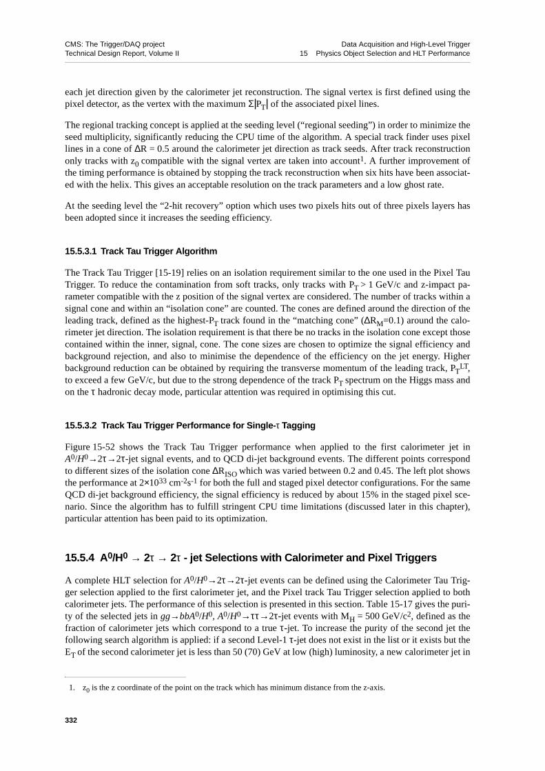
CMS: The Trigger/DAQ project Data Acquisition and High-Level TriggerTechnical Design Report, Volume II 15 Physics Object Selection and HLT Performance
each jet direction given by the calorimeter jet reconstruction. The signal vertex is first defined using thepixel detector, as the vertex with the maximum Σ|PT| of the associated pixel lines.
The regional tracking concept is applied at the seeding level (“regional seeding”) in order to minimize theseed multiplicity, significantly reducing the CPU time of the algorithm. A special track finder uses pixellines in a cone of ∆R = 0.5 around the calorimeter jet direction as track seeds. After track reconstructiononly tracks with z0 compatible with the signal vertex are taken into account1. A further improvement ofthe timing performance is obtained by stopping the track reconstruction when six hits have been associat-ed with the helix. This gives an acceptable resolution on the track parameters and a low ghost rate.
At the seeding level the “2-hit recovery” option which uses two pixels hits out of three pixels layers hasbeen adopted since it increases the seeding efficiency.
15.5.3.1 Track Tau Trigger Algorithm
The Track Tau Trigger [15-19] relies on an isolation requirement similar to the one used in the Pixel TauTrigger. To reduce the contamination from soft tracks, only tracks with PT > 1 GeV/c and z-impact pa-rameter compatible with the z position of the signal vertex are considered. The number of tracks within asignal cone and within an “isolation cone” are counted. The cones are defined around the direction of theleading track, defined as the highest-PT track found in the “matching cone” (∆RM=0.1) around the calo-rimeter jet direction. The isolation requirement is that there be no tracks in the isolation cone except thosecontained within the inner, signal, cone. The cone sizes are chosen to optimize the signal efficiency andbackground rejection, and also to minimise the dependence of the efficiency on the jet energy. Higherbackground reduction can be obtained by requiring the transverse momentum of the leading track, PT
LT,to exceed a few GeV/c, but due to the strong dependence of the track PT spectrum on the Higgs mass andon the τ hadronic decay mode, particular attention was required in optimising this cut.
15.5.3.2 Track Tau Trigger Performance for Single-τ Tagging
Figure 15-52 shows the Track Tau Trigger performance when applied to the first calorimeter jet inA0/H0→2τ→2τ-jet signal events, and to QCD di-jet background events. The different points correspondto different sizes of the isolation cone ∆RISO which was varied between 0.2 and 0.45. The left plot showsthe performance at 2×1033 cm-2s-1 for both the full and staged pixel detector configurations. For the sameQCD di-jet background efficiency, the signal efficiency is reduced by about 15% in the staged pixel sce-nario. Since the algorithm has to fulfill stringent CPU time limitations (discussed later in this chapter),particular attention has been paid to its optimization.
15.5.4 A0/H0 → 2τ → 2τ - jet Selections with Calorimeter and Pixel Triggers
A complete HLT selection for A0/H0→2τ→2τ-jet events can be defined using the Calorimeter Tau Trig-ger selection applied to the first calorimeter jet, and the Pixel track Tau Trigger selection applied to bothcalorimeter jets. The performance of this selection is presented in this section. Table 15-17 gives the puri-ty of the selected jets in gg→bbA0/H0, A0/H0→ττ→2τ-jet events with MH = 500 GeV/c2, defined as thefraction of calorimeter jets which correspond to a true τ-jet. To increase the purity of the second jet thefollowing search algorithm is applied: if a second Level-1 τ-jet does not exist in the list or it exists but theET of the second calorimeter jet is less than 50 (70) GeV at low (high) luminosity, a new calorimeter jet in
1. z0 is the z coordinate of the point on the track which has minimum distance from the z-axis.
332

CMS: The Trigger/DAQ project Data Acquisition and High-Level TriggerTechnical Design Report, Volume II 15 Physics Object Selection and HLT Performance
the region centred on first Level-1 Central jet is reconstructed. The purity of the second jet when chosenin such a way is increased to ~90% (the numbers in parentheses in Table 15-17 correspond to the purity ofthe selection when this re-definition algorithm is not applied).
Usage of the Calorimeter Tau Trigger as a pre-selector before applying the Pixel track Tau Trigger allowsconsiderable reduction of the total CPU time per event. The cuts are optimized by examining the back-ground rejection, Scalo, of the Calorimeter Tau Trigger step, the efficiency for the signal, and the CPUtime usage, while keeping a suppression factor of the full High-Level Trigger selection of ~ 103. Resultsof such a study for MH = 200 GeV/c2 are presented in Table 15-18 for the low luminosity scenario withthe full pixel system. It has been found that for for a total suppression factor of 103, at both low and highluminosity, a calorimeter suppression factor of three yields the highest signal efficiency. At this operatingpoint the total time Ttot of the full path is 59 ms for low luminosity and 174 ms for high luminosity.
Figure 15-52 Efficiency of Track Tau Trigger for the first calorimeter jet in A0/H0 → 2τ → 2τ - jet, for two Higgsmasses, MH = 200 and 500 GeV/c2, versus the efficiency for QCD di-jet background events. Left: at a luminosityof 2×1033cm-2s-1, for both the full and the staged pixel systems, and right: at 1034cm-2s-1.
Table 15-17 Purity of calorimeter jets in events at low and high lumi-nosity. Numbers for the 2nd jet without (with) parentheses are thepurity after (before) re-definition of the 2nd jet.
L=2×1033cm-2s-1 L=1034cm-2s-1
1st jet 2nd jet 1st jet 2nd jet
0.98 0.90 (0.63) 0.98 0.88 (0.65)
Table 15-18 Efficiency for A0/H0 → 2τ → 2τ - jet events, and total CPU time, as a function of the Calorimeterisolation cut and its background rejection factor at a luminosity of 2×1033cm-2s-1. An overall suppression factor103 for background events is maintained. The bolded column corresponds to the operating point.
Cut on the isolation parameter Pisol, GeV - 10.4 7.6 5.6 4.6 4.0 3.4 3.2 2.6
Background rejection factor, Scalo 1.0 1.5 2.0 3.0 4.0 5.0 6.2 7.5 10.0
Ttot=Tcalo + Tpixel / Scalo (ms) 110 85 72 59 52 50 45 43 41
Efficiency of Calo + Pixel Tau selection 0.35 0.37 0.40 0.41 0.40 0.39 0.37 0.36 0.35
0.4
0.5
0.6
0.7
0.8
0.9
1
0 0.02 0.04 0.06 0.08 0.1 0.12 0.14 0.16 0.18
ε(QCD 50-170 GeV)
ε(H
(200
,500
GeV
)→ττ
,τ→1,
3h+X
)
MH=200 GeV, staged Pxl
MH=500 GeV, staged Pxl
MH=200 GeV, not staged Pxl
MH=500 GeV, not staged Pxl
MH=200 GeV
MH=500 GeV
RM=0.1
L=2x1033cm-2s-1
PTLT>6 GeV
RS=0.07, RI is varied 0.2 - 0.45Trk Tau Trigger on first Calo jet
0.4
0.5
0.6
0.7
0.8
0.9
1
0 0.02 0.04 0.06 0.08 0.1 0.12 0.14 0.16 0.18
ε(QCD 50-170 GeV)
ε(H
(200
,500
GeV
)→ττ
,τ→1,
3h+X
)
MH=200 GeV
MH=500 GeV
RM=0.1
L=1034cm-2s-1, not staged Pxl
PTLT>7 GeV
RS=0.065, RI is varied 0.2 - 0.45Trk Tau Trigger on first Calo jet
333

CMS: The Trigger/DAQ project Data Acquisition and High-Level TriggerTechnical Design Report, Volume II 15 Physics Object Selection and HLT Performance
Figure 15-54 shows the efficiency of the Calorimeter+Pixel track Tau Trigger selection for the signal andfor QCD di-jet background events at low and high luminosity. The size of the isolation cone ∆Ri is variedin the range 0.20 to 0.50, and the optimal suppression factor of 3 for the Calorimeter Tau Trigger is used.For a total suppression factor of ~103, there is little difference in efficiency between the staged and fullpixel configurations at low luminosity.
15.5.5 A0/H0 → 2τ → 2τ - jet Selections with Track Tau Trigger.
In this section the performance of a complete HLT selection for A0/H0→2τ→2τ-jet is discussed, when theCalorimeter Tau Trigger selection, applied on the first calorimeter jet, is followed by the Track Tau Trig-ger on both calorimeter jets (Calo+Track Tau Trigger path). Figure 15-54 shows the signal vs. back-ground algorithmic efficiency when the Track Tau Trigger selection is applied to both calorimeter jets, atlow luminosity (left plot), for both the complete and staged pixel detector, and at high luminosity (rightplot). The different points correspond to different sizes of the isolation cone, ∆RISO, which is varied be-tween 0.2 and 0.45. At a QCD di-jet background efficiency of ~10-3 the signal efficiency with the stagedpixel detector is reduced by about 20%. A cut on PT on the leading track of 6 (7) GeV/c is required at low(high) luminosity to reach a background rejection factor ~103.
Figure 15-54 shows the algorithmic efficiency of the signal vs that of the background when the Calorime-ter Tau Trigger selection, applied on the first calorimeter jet, is followed by the Track Tau Trigger on bothcalorimeter jets (Calo+Track Tau Trigger path). Table 15-19 summarizes the efficiency of the Track TauTrigger at the operating points where the background rejection factor is ~103. These points have beenchosen taking into account the overall performance and minimizing the τ-jet energy dependency of thesignal efficiency. The third and fifth rows of Table 15-19 list the efficiency at low and high luminosity forthe full Calo+Track Tau Trigger selection.
The Track Tau Trigger CPU time distribution is shown in Figure 15-56 for Higgs and QCD di-jet back-ground events at low luminosity. The time needed for a double tag is only slightly larger than the time
Figure 15-53 Efficiency of the Calo+Pxl Tau Trigger path for A0/H0 → 2τ → 2τ - jet and QCD 2-jet backgroundevents when the size of the isolation cone Ri is varied in the range 0.20-0.50. The optimal suppression factor ofthree for the Calo Tau Trigger is taken. Results for two Higgs masses, MH=200 and 500 GeV/c2, are shown. Left:L=2×1033cm-2s-1, with the full and staged pixel systems. Right: L=1034cm-2s-1.
0.2
0.25
0.3
0.35
0.4
0.45
0.5
0.55
0.6
0.65
0.7
10-3
10-2
ε(QCD bkg 50-170 GeV)
ε(H
(200
, 500
GeV
)→ττ
, τ→
1,3h
+X
)
L=1034cm-2s-1
Calo+Pxl Tau Trigger
RS=0.07, RI is varied 0.2-0.5
RM=0.10
Pem=9.8 GeV
MH=200 GeV
MH=500 GeV
0.2
0.25
0.3
0.35
0.4
0.45
0.5
0.55
0.6
0.65
0.7
10-3
10-2
ε(QCD bkg 50-170 GeV)
ε(H
(200
, 500
GeV
)→ττ
, τ→
1,3h
+X)
Calo+Pxl Tau Trigger
L=2×1033cm-2s-1
RS=0.07, RI is varied 0.2-0.5
RM=0.10
Pem=5.6 GeV
MH=200 GeV, not staged Pxl
MH=500 GeV, not staged Pxl
MH=200 GeV, staged Pxl
MH=500 GeV, staged Pxl
334

CMS: The Trigger/DAQ project Data Acquisition and High-Level TriggerTechnical Design Report, Volume II 15 Physics Object Selection and HLT Performance
needed for a single tag, since the second calorimeter jet is analysed only in the ~ 6% of background eventswhich pass the single tag on the first calorimeter jet. Only 10% of the QCD events require more than400 ms to be analysed.
An important advantage of the Calo+Track Tau Trigger selection over the simple Track Tau Trigger is itsbetter time performance, which is due to the fact that only those events which pass the calorimeter τ selec-tion on the first jet need to be analysed by the Track Tau Trigger. Following the same method described inSection 15.5.4 and using the numbers from Table 15-18 (Scalo = 3, Tcalo ≅ 33 ms) an average time ofabout 130 ms/event is expected at low luminosity.
The time required by the Track Tau Trigger at high luminosity is much larger and is currently estimated at≅ 1 s/event. However, making use of the Calo+Track Tau Trigger selection, this time will be less than400 ms/event, which is acceptable. A further improvement is expected with the use of a regional pixel re-construction.
Figure 15-54 Efficiency of Track Tau Trigger applied to both Calo jets in A0/H0 → 2τ → 2τ - jet vs that in QCDdi-jet event. Left: for L = 2×1033cm-2s-1, for both the full and staged pixel systems. Right: for L = 1034cm-2s-1.Two Higgs masses MH = 200 and 500 GeV/c2, are shown.
Table 15-19 Summary of Track Tau Trigger efficiency when two Calo jets are tagged. A QCD di-jet backgroundrejection (last column) of ~103 is required. The third and fifth rows show the results when the Calorimeter TauTrigger selection applied on the first Calo jet is followed by the Track Tau Trigger on both Calo jets. Due to thelimited Monte Carlo statistics some statistical errors for the QCD background are large.
Luminosity Configuration/Trigger MH = 200 GeV/c2 MH = 500 GeV/c2 QCD
2×1033cm-2s-1 Staged pixels, Track Tau 0.355±0.006 0.375±0.005 (8.6±1.6)×10-4
2×1033cm-2s-1 Full pixels, Track Tau 0.433±0.006 0.489±0.005 (8.3±1.6)×10-4
2×1033cm-2s-1 Full pixels, Calo+Track Tau 0.446±0.006 0.486±0.005 (1.0±0.2)×10-3
1034cm-2s-1 Track Tau 0.346±0.006 0.420±0.005 (1.13±0.4)×10-3
1034cm-2s-1 Calo + Track Tau 0.361±0.006 0.427±0.005 (9.4±3.0)×10-4
0.2
0.25
0.3
0.35
0.4
0.45
0.5
0.55
0.6
0.65
0.7
10-3
10-2
ε(QCD 50-170 GeV)
ε(H
(200
,500
GeV
)→ττ
,τ→1,
3h+X
)
MH=200 GeV, staged Pxl
MH=500 GeV, staged Pxl
MH=200 GeV, not staged Pxl
MH=500 GeV, not staged Pxl
MH=200 GeV
MH=500 GeV
PTLT>6 GeV
RS=0.07, RI is varied 0.2 - 0.45
RM=0.1
L=2x1033cm-2s-1
Trk Tau Trigger
0.2
0.25
0.3
0.35
0.4
0.45
0.5
0.55
0.6
0.65
0.7
10-3
10-2
ε(QCD 50-170 GeV)ε(
H(2
00,5
00 G
eV)→
ττ,τ→
1,3h
+X)
MH=200 GeV
MH=500 GeV
PTLT>7 GeV
RS=0.065, RI is varied 0.2 - 0.45
RM=0.1
L=1034cm-2s-1, not staged PxlTrk Tau Trigger
335
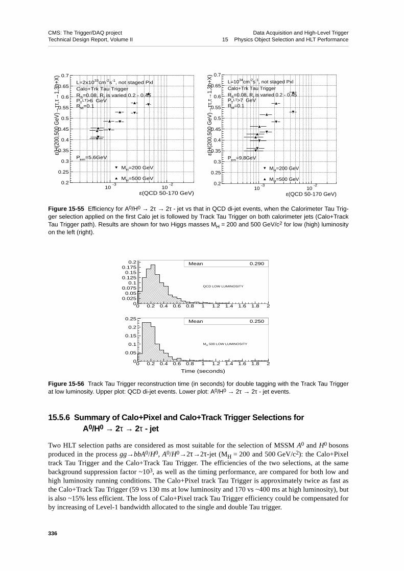
CMS: The Trigger/DAQ project Data Acquisition and High-Level TriggerTechnical Design Report, Volume II 15 Physics Object Selection and HLT Performance
15.5.6 Summary of Calo+Pixel and Calo+Track Trigger Selections for A0/H0 → 2τ → 2τ - jet
Two HLT selection paths are considered as most suitable for the selection of MSSM A0 and H0 bosonsproduced in the process gg→bbA0/H0, A0/H0→2τ→2τ-jet (MH = 200 and 500 GeV/c2): the Calo+Pixeltrack Tau Trigger and the Calo+Track Tau Trigger. The efficiencies of the two selections, at the samebackground suppression factor ~103, as well as the timing performance, are compared for both low andhigh luminosity running conditions. The Calo+Pixel track Tau Trigger is approximately twice as fast asthe Calo+Track Tau Trigger (59 vs 130 ms at low luminosity and 170 vs ~400 ms at high luminosity), butis also ~15% less efficient. The loss of Calo+Pixel track Tau Trigger efficiency could be compensated forby increasing of Level-1 bandwidth allocated to the single and double Tau trigger.
Figure 15-55 Efficiency for A0/H0 → 2τ → 2τ - jet vs that in QCD di-jet events, when the Calorimeter Tau Trig-ger selection applied on the first Calo jet is followed by Track Tau Trigger on both calorimeter jets (Calo+TrackTau Trigger path). Results are shown for two Higgs masses MH = 200 and 500 GeV/c2 for low (high) luminosityon the left (right).
Figure 15-56 Track Tau Trigger reconstruction time (in seconds) for double tagging with the Track Tau Triggerat low luminosity. Upper plot: QCD di-jet events. Lower plot: A0/H0 → 2τ → 2τ - jet events.
0.2
0.25
0.3
0.35
0.4
0.45
0.5
0.55
0.6
0.65
0.7
10-3
10-2
ε(QCD 50-170 GeV)
ε(H
(200
,500
GeV
)→ττ
,τ→1,
3h+X
)
MH=200 GeV
MH=500 GeV
PTLT>6 GeV
RS=0.08, RI is varied 0.2 - 0.45
RM=0.1
L=2x1033cm-2s-1, not staged PxlCalo+Trk Tau Trigger
Pem=5.6GeV
0.2
0.25
0.3
0.35
0.4
0.45
0.5
0.55
0.6
0.65
0.7
10-3
10-2
ε(QCD 50-170 GeV)
ε(H
(200
,500
GeV
)→ττ
,τ→1,
3h+X
)
MH=200 GeV
MH=500 GeV
PTLT>7 GeV
RS=0.08, RI is varied 0.2 - 0.45
RM=0.1
L=1034cm-2s-1, not staged PxlCalo+Trk Tau Trigger
Pem=9.8GeV
00.025
0.050.075
0.10.125
0.150.175
0.2
0 0.2 0.4 0.6 0.8 1 1.2 1.4 1.6 1.8 2
Mean 0.290
QCD LOW LUMINOSITY
0
0.05
0.1
0.15
0.2
0.25
0 0.2 0.4 0.6 0.8 1 1.2 1.4 1.6 1.8 2
Mean 0.250
Time (seconds)
MH 500 LOW LUMINOSITY
336

CMS: The Trigger/DAQ project Data Acquisition and High-Level TriggerTechnical Design Report, Volume II 15 Physics Object Selection and HLT Performance
15.5.7 H+ → τν → τ - jet Selections with Track Tau Trigger.
The Track Tau Trigger will work as the final part of the selection MSSM charged Higgs bosons in theprocess gb(g)→H+t(b), H+→τν→τ-jet, t→bjj. The Level-1 single-τ trigger followed by a HLT selectionof events with ET
miss > 65 (95) GeV at low (high) luminosity gives an output rate of about 30 (70) Hz.The selection must provide a suppression factor of ~30 to match the output bandwidth requirements. TheTrack Tau Trigger selection is applied to the calorimeter jet reconstructed in the region of the first Level-1τ-jet. The purity of the calorimeter jet in signal events is 85%.
The isolation criteria used in the Pixel or Track Tau Triggers cannot provide the required suppression fac-tor. Additional background rejection is obtained by applying a cut on the PT of the leading track in theTrack Tau Trigger . Figure 15-57 shows the Track Tau Trigger efficiencies for the signal and QCD back-ground passing the Level-1 single-τ trigger. Since the cut on ET
miss and the Track Tau selection efficiencyare uncorrelated [15-19], a cut on ET
miss has not been applied due to limited Monte Carlo statistics.
The different points in Figure 15-57 correspond to varying the cut on the PT of the leading track, PTLT,
from 1 to 30 GeV/c. A rejection factor 30 can be reached with a 20 (25) GeV/c cut on PTLT at low (high)
Figure 15-57 Track Tau Trigger efficiency for H+→τν→τ-jet events vs the QCD di-jet background efficiency.The results are given for MH = 200 GeV/c2 and MH = 400 GeV/c2. Isolation parameters are: ∆RM = 0.1,∆RSIG = 0.065 (0.060) for low (high) luminosity, ∆RISO = 0.4; cut on PT of the leading track is varied from 1 to30 GeV/c. Left plot: L = 2×1033cm-2s-1, with the full pixel system; Right plot: L = 1034cm-2s-1.
Table 15-20 Track Tau Trigger efficiency for the process gb(g)→H+t(b), H+→τν→τ-jet, t→bjj and for the QCDbackground. The efficiencies for the signal are presented for a background suppression factor of ~30.
Signal and background samples Efficiency of Track Tau Trigger
Low LuminosityPT
LT > 20 GeV/c∆RSIG=0.065
High LuminosityPT
LT > 25 GeV/c ∆RSIG = 0.06
H+→τν MH= 200 GeV/c2 0.580 ± 0.004 0.534 ± 0.005
MH= 400 GeV/c2 0.579 ± 0.004 0.553 ± 0.006
QCD 50 < PT < 170 GeV/c 0.031 ± 0.002 0.028 ± 0.003
0.45
0.5
0.55
0.6
0.65
0.7
0.75
0.01 0.02 0.03 0.04 0.05 0.06 0.07
ε(QCD 50-170 GeV)
ε(H
(200
,400
GeV
)→τν
,τ→1,
3h+X
)
L=2x1033cm-2s-1, not staged Pxl
Trk Tau TriggerPT
LT is varied 1.-30. GeVRM = 0.1
RS = 0.065, RI=0.4
MH=400 GeV
MH=200 GeV
0.45
0.5
0.55
0.6
0.65
0.7
0.75
0.01 0.02 0.03 0.04 0.05 0.06 0.07
ε(QCD 50-170 GeV)
ε(H
(200
,400
GeV
)→τν
,τ→1,
3h+X
)
L=1034cm-2s-1, not staged Pxl
Trk Tau TriggerPT
LT is varied 1.-30. GeVRM = 0.1
RS = 0.06, RI=0.4
MH=400 GeV
MH=200 GeV
337

CMS: The Trigger/DAQ project Data Acquisition and High-Level TriggerTechnical Design Report, Volume II 15 Physics Object Selection and HLT Performance
luminosity, which is well below the foreseen offline analysis cut [15-15]. Table 15-20 summarizes the ef-ficiency of the Track Tau Trigger at this working point with a background rejection factor of 30.
15.5.8 Triggering on Mixed Channels: A0/H0 → 2τ → e + τ - jet
The triggering scheme for gg→bbA0/H0, A0/H0→2τ→e+τ-jet has been studied for MH = 200 GeV/c2.The trigger accepts events which pass either a single-e or a combined e+τ-jet (‘eTau’) trigger. In what fol-lows the combined trigger will be called the ‘e+eTau’ trigger. The eTau trigger requires the presence ofboth an electron and a τ-jet, with thresholds lower than those used in the single-e and single-τ-jet triggers.The τ-jet candidate at Level-1 is defined as the most energetic τ-jet that is not collinear with the electroncandidate (∆R > 0.3). This condition avoids misidentification in signal events (the τ purity in signalevents increases from 61% to 99%) with little influence on the overall efficiency.
15.5.8.1 High Luminosity
Figure 15-58 shows the Level-1 ‘e+eTau’ trigger rate at 1034 cm-2s-1 as a function of the electron andτ-jet thresholds used in the eTau trigger. The dots with numbers on the ‘e+eTau’ trigger isorate curves in-dicate the Level-1 selection efficiency for the signal. For a given Level-1 trigger rate, the efficiency in-creases when the electron threshold is reduced and the τ-jet threshold is raised. This results from thesteeply falling PT spectrum of the electron in the signal channel. Figure 15-59 shows the increase in Lev-el-1 efficiency obtained by using the ‘e+eTau’ trigger, as opposed to just the single electron trigger, as afunction of the extra bandwidth which one devotes to the eTau trigger. The curves are each obtained byfixing the threshold for the electron in eTau trigger and varying the threshold on τ-jet.
Figure 15-58 Level-1 ‘e+eTau’ trigger rate at a luminosity of 1034cm-2s-1 as a function of the e and τ-jet thresh-olds, for a fixed single-e trigger threshold. The four curves correspond to additional bandwidths of 0.14 kHz,0.39 kHz, 0.85 kHz and 1.28 kHz, respectively, being devoted to the eTau trigger, on top of the constant6.54 kHz devoted to the single-e trigger. The vertical line at 28 GeV corresponds to the single-e trigger. The val-ues listed in the upper right corner are the rates and efficiencies for the single-e trigger at Level-1, Level-2.0 andLevel-2.5.
L1 electron Et Cut (GeV)18 20 22 24 26 28 30 32
L1
tau
jet
Et
Cu
t (G
eV)
55
60
65
70
75
80
85
9063.4%
62.7%
61.8%
60.3%
66.0%
64.4%
62.8%
67.5%
65.6%68.5%
7 kHz
6.7 kHz
7.5 kHz
8.0 kHz
L1 Rate = 6535 HzL2 Rate = 3364HzL25 Rate= 333 Hz
L1 Effi = 58.4 %L2 Effi = 51.6 %L25 Effi= 44.6 %
L1 Rate and efficiencyL=1034 cm-2s-1
338

CMS: The Trigger/DAQ project Data Acquisition and High-Level TriggerTechnical Design Report, Volume II 15 Physics Object Selection and HLT Performance
The HLT selection is applied independently on the electron stream and the eTau stream at Level-2.0 andLevel-2.5. At Level-2.0, a threshold is applied only on the electron candidate (Section 15.2.4). At Lev-el-2.5, pixel/super-cluster matching is used for the electron candidate (Section 15.2.5) and the τ-jet identi-fication is applied as described in Section 15.5.2.
Table 15-21 shows the details of the full selection for four scenarios. In both cases, the eTau trigger usesan electron threshold corresponding to 25.5 GeV on the Level-1 95% efficiency scale, while the τ thresh-old is varied in such a way that the rate added by the eTau trigger to the single-electron trigger rate is0.14 kHz, 0.39 kHz, 0.85 kHz and 1.28 kHz respectively. Accepting an additional rate of 0.85 kHz atLevel-1 leads to a relative improvement in efficiency, at Level-2.5, of about 10% at a price of a 7 Hz rateincrease. This is illustrated in Figure 15-60 which shows the PT spectrum of the electron that is recoveredat Level-2.5 when the eTau trigger is added to the single electron trigger at Level-1.
15.5.8.2 Low Luminosity
Since the single electron thresholds are lower in the low luminosity scenario, less is gained by adding thecombined eTau Trigger. The HLT selection scheme is the same as at high luminosity but the Level-1thresholds are different. For a scenario where 0.82 kHz for the eTau trigger is added at Level-1, the rela-tive gain in efficiency at Level-2.5 is ~4%.
15.5.9 Triggering on Mixed Channels: A0/H0 → 2τ → µ + τ - jet
The reconstruction efficiencies and online background rejection performance for A0/H0→2τ→µ+τ-jethave been studied for the case when the Higgs particle is produced in association with b-quarks and themass of Higgs particle is rather low (200 GeV/c2). The focus is on the high-luminosity case, where the
Figure 15-59 The increase in Level-1 efficiency, at1034cm-2s-1, obtained using the ‘e+eTau’ trigger, asopposed to just the single electron trigger, as a func-tion of the extra band-width devoted to the eTau trig-ger. Each curve is obtained by fixing the e threshold(ET
e in the plot) and varying the threshold for the τ-jet.
Figure 15-60 Electron PT in A0/H0 → 2τ → e+τ - jetevents, at 1034cm-2s-1. The filled portion of the histo-gramme corresponds to the gain observed atLevel-2.5 by adding the Level-1 e+τ trigger, theremaining unfilled part corresponds to electrons pass-ing the single electron trigger.
Level-1 Additionnal Rate (Hz)0 500 1000 1500 2000 2500
0
0.05
0.1
0.15
0.2
L=1034 cm-2s-1Et ≥18 GeV
e
Et ≥19 GeVe
Et ≥20 GeVe
Et ≥21 GeVe
Et ≥22 GeVe
Et ≥23 GeVe
(ε[e
or
eT
au
]-ε[
e])
/ε[e
] a
t L
ev
el-
1
Et ≥24 GeVe
Et ≥25 GeVe
Et ≥26 GeVe
Et ≥27 GeVe
Et ≥28 GeVe
Electron Pt (GeV/c)0 20 40 60 80 100 120 140
0
50
100
150
200
250 Spectrum recovery at L25L=1034 cm-2s-1
339

CMS: The Trigger/DAQ project Data Acquisition and High-Level TriggerTechnical Design Report, Volume II 15 Physics Object Selection and HLT Performance
event selection and background reduction are more difficult. The quoted efficiencies are given with re-spect to “useful” events defined using Monte-Carlo parameters (PT
µ > 14 GeV/c, PTτ-jet > 30 GeV/c,
|ηµ,τ-jet| < 2.4), and which select 45% of all H→µ+τ-jet generated decays. Due to the relatively lowthreshold of the Level-1 single-µ trigger (PT
cut = 20 GeV/c), about 66% of the useful events are taken bythe Level-1 single-µ or Level-1 single-τ triggers as shown in Figure 15-61.
Table 15-21 Evolution of the rate and the efficiency of the different trigger levels at high luminosity. Results forfour different tau thresholds in the eTau trigger are shown, as are results obtained with no eTau trigger (just thesingle electron trigger).
e + eTau trigger e trigger
L1 eTau thresh (GeV) (20, 57) (20, 62) (20, 72) (20, 89) (28)
L1 Rate (Hz) 7819 7389 6933 6677 6535
L1 Additional Rate (Hz) 1284 854 398 142
L1 Efficiency 0.685 0.675 0.661 0.634 0.584
L1 Additional Efficiency 0.101 0.091 0.077 0.050
L2.0 Rate (Hz) 4219 3945 3631 3452 3364
L2.0 Additional Rate (Hz) 855 581 267 88
L2.0 Efficiency 0.614 0.605 0.590 0.562 0.5165
L2.0 Additional Efficiency 0.098 0.089 0.074 0.046
L2.5 Rate (Hz) 343 339 338 333 332
L2.5 Additional Rate (Hz) 11 7 6 1
L2.5 Efficiency 0.492 0.489 0.483 0.469 0.446
L2.5 Additional Efficiency 0.046 0.043 0.037 0.023
Figure 15-61 The PT spectrum of generated muons (left) and the ET spectrum of generated τ-jets (right). Theevents accepted by the µ−τ Level-1 Trigger (with combined threshold PT ≥ 14 GeV/c, ET ≥ 45 GeV) are shownon the top of useful events. The fraction of Level-1 events accepted by single-µ or single-τ trigger is indicated.
[GeV/c]Tgenerated muon p0 20 40 60 80 100
arb
itra
ry u
nit
s
useful events
L1 accepted
L1 accepted && L1 mu
L1 accepted && L1 tau
[GeV]Tgenerated tau-jet E0 20 40 60 80 100 120 140 160 180 200
arb
itra
ry u
nit
s
useful events
L1 accepted
L1 accepted && L1 mu
L1 accepted && L1 tau
340

CMS: The Trigger/DAQ project Data Acquisition and High-Level TriggerTechnical Design Report, Volume II 15 Physics Object Selection and HLT Performance
In Figure 15-62, the efficiency of the Level-1 µ−τ trigger is shown as a function of µ PT and τ ET. Onlyevents where both the τ−jet and the µ are found by the trigger (irrespective of their PT and ET) contributeto the plot. The combined trigger increases the efficiency by up to a maximum of 73% for the loose PTand ET cuts. In order to preserve events passing the offline cuts PT > 15 GeV/c, ET ≥ 40 GeV, one canchoose the corresponding Level-1 working point with Level-1 PT ≥ 14 GeV/c and Level-1 ET > 45 GeVwith an overall efficiency of 70%.
The additional rate taken by the Level-1 combined µ−τ-jet trigger over that of the single-µ trigger(~6 kHz) and single τ-jet trigger (~2 kHz) is shown in Figure 15-63. The additional rate for the proposedworking point is 0.83 kHz. The full rate for events selected by the combined trigger (both Level-1 µ andLevel-1 τ found) passing the single-µ, single τ-jet or combined thresholds is 5.8 kHz.
The HLT analysis in this channel consists of:
• identification of Level-2 jet corresponding to Level-1 τ-jet with a ET cut;
• calorimeter isolation cut for the τ;
• Level-2 µ identification and PT cut;
• calorimeter isolation cut for the µ;
• Level-3 µ identification and PT cut
• τ-jet identification and isolation requirement in the pixel detector
• µ isolation cut with full tracker (or with pixel detector)
The resulting HLT efficiencies and rates are shown in Figure 15-64 as the function of the HLT cuts. Onlyevents passing the proposed Level-1 thresholds are included. Setting the HLT thresholds at the offline val-ues preserves 32% of events in the reference useful sample. The corresponding rate from the muon mini-
Figure 15-62 Level-1 Trigger efficiency as the func-tion of the cuts for high luminosity. µ−τ events taken bythe single-µ or single-τ trigger are included. The differ-ence between contour lines represents a change inefficiency of 1%. The Level-1 cut corresponding to theoffline cut selects ~70% of the reference events.
Figure 15-63 Level-1 Trigger rate at high luminosityfrom µ−τ events. This rate is in addition to the Level-1single-µ and Level-1 single-τ trigger rates. The addi-tional rate, for the Level-1 cut that corresponds to theoffline cut, is 0.83 kHz.
cut [GeV/c]TL1 muon p0 5 10 15 20 25
cu
t [G
eV]
TL
1 ta
u E
0
20
40
60
80
100
120
140
0.698
0.66
0.66
0.66
0.73
effic > 70 %
cut [GeV/c]TL1 muon p0 5 10 15 20 25
cu
t [G
eV]
TL
1 ta
u E
0
20
40
60
80
100
120
140
833 Hz
4.5e+05 Hz
rate > 1 Hz
rate > 3 Hz
rate > 10 Hz
rate > 30 Hz
rate > 100 Hz
rate > 300 Hz
rate > 1 kHz
rate > 3 kHz
rate > 10 kHz
341

CMS: The Trigger/DAQ project Data Acquisition and High-Level TriggerTechnical Design Report, Volume II 15 Physics Object Selection and HLT Performance
mum-bias samples is about 1 Hz. The detailed list of rejection factors and efficiencies for each HLT stepis given in Table 15-22.
The low-luminosity case is simpler. The Level-1 single-µ threshold of 12 GeV/c is below the offline cutand there is no need to allocate bandwidth to the µ+τ-jet channel. The Level-1 single-µ and single-τ trig-gers (ET >93 GeV) select about 72% of the events in the sample. The µ and τ identification and selectioncriteria in the HLT reduce this efficiency to 39% with a background rate of 0.2 Hz.
Figure 15-64 Full selection (Level-1 + HLT) in H→ τ τ → µ + τ−jet channel. The selection efficiency (left) andcorresponding background rate (right) are shown. The Level-1 combined µ−τ cut is at µ Level-1 PT = 14 GeV/cand Level-1 τ-jet ET = 45 GeV. Events must pass Level-1 and all HLT µ and τ selection requirements. The tau95% efficiency scale is used for tau ET. The µ 90% efficiency scale is used for µ PT.The efficiency and rate forthe offline threshold (PT = 15 GeV/c, ET = 40 GeV) are marked.
Table 15-22 Summary of Level-1 and HLT selection efficiencies and background rates in the H→2τ→µ+τ-jetchannel for the thresholds corresponding to the offline cut at PT = 15 GeV/c, ET = 40 GeV. The efficiency isdefined with respect to all events in the useful sample.
Efficiency Rate [Hz]
Events passing Level-1 single µ, single τ, or combined trigger 0.70 5.8×10³
Events passing Level-1 combined trigger not selected by single-µ or single-τ trigger 0.04 830
L2 identification with ET and PT cuts 0.63 990
L2 and calo tau isolation 0.53 380
L2 and muon calo isolation 0.61 420
L2 combined 0.51 150
L3 identification with µ PT cut 0.49 59
L3 and tau isolation 0.33 3.4
L3 and muon isolation 0.48 25
L3 combined 0.32 1.2
cut [GeV/c]Tmuon p0 5 10 15 20 25 30 35 40
cu
t [G
eV]
Tta
u E
0
10
20
30
40
50
60
70
80
90
0.32
0.35
effic > 10 %
effic > 20 %
effic > 30 %
cut [GeV/c]Tmuon p0 5 10 15 20 25
cu
t [G
eV]
Tta
u E
0
10
20
30
40
50
60
1.2 Hz
22.7 Hz
rate > 1 Hz
rate > 3 Hz
rate > 10 Hz
342

CMS: The Trigger/DAQ project Data Acquisition and High-Level TriggerTechnical Design Report, Volume II 15 Physics Object Selection and HLT Performance
15.5.10 Summary of Level-1 and HLT for Higgs Channels with τ-leptons.
The following Level-1 and HLT paths are used to trigger on the MSSM A0/H0 and H+ Higgs bosons withmass greater than 200 GeV/c2:
1. A/H→ττ→2τ-jets. At Level-1: single and double τ-jet; at HLT: calorimeter + tracker isolation.
2. H+→τν→τ-jet+ETmiss. At Level-1: single τ-jet; at HLT : calorimeter ET
miss and tracker isolationon the τ-jet.
3. A/H→ττ→e+τ-jet. At Level-1: single-e and combined e+τ-jet triggers; at HLT: electron selectionas described in Section 15.2 and τ-jet isolation with the tracker.
4. A/H→ττ→µ+τ-jet. At Level-1: single-µ and combined µ+τ-jet triggers; at HLT: muon selectionsas described in Section 15.3 and τ-jet isolation with the calorimeter and the tracker.
The HLT output rates, the signal efficiency (for MH=200 GeV/c2) of the Level-1 and HLT selections aswell as the CPU usage at both low and high luminosity are listed in Table 15-23
The efficiency of the combined triggers used for A/H→ττ→lepton+τ-jet channels are only about 2-5 %higher than those of the single-lepton trigger. This is mostly due to the choice of a relatively high mass forthe Higgs bosons. As an example, for Higgs masses around 120 GeV/c2, the fusion channel qq→qqH,H→ττ can benefit significantly from a combined trigger.
Table 15-23 The efficiency of the Level-1 and HLT selections, the HLT output rates and CPU usage for low andhigh luminosity (numbers in parentheses) for the MSSM Higgs to t decays discussed in the text.
ChannelLevel-1
efficiency (%)HLT output rate
(Hz) HLT efficiency (%) HLT CPU (ms)
A/H→ττ→2τ-jets 78 (62) 3 (8) 45 (36) 130
H+→τν→τ-jet+ETmiss 81 (76) 1 (2) 58 (53) 38
A/H→ττ→µ+τ-jet 72 (70) 0.2 (1.2) 54 (46) 660
A/H→ττ→e+τ-jet 80 (69) 0.4 (1.8) 70 (71) 165
343

CMS: The Trigger/DAQ project Data Acquisition and High-Level TriggerTechnical Design Report, Volume II 15 Physics Object Selection and HLT Performance
15.6 b-jet Identification
Many physics channels contain hard b-jets in the final state which are hidden by the more copious lightflavoured jets. Inclusive b-tagging of jet triggers can be used for selection of these channels. The algo-rithms used for b-tagging rely on the large value of the b-hadron proper time (cτ~450 µm), which givesrise to tracks with large impact parameters with respect to the production vertex.
15.6.1 Tagging Algorithm
The algorithms which will run at the HLT stage should be robust and fast. A wide range of algorithmshave been developed within CMS to tag b-jets [15-20]. The tag chosen for these studies relies upon thetrack impact parameter.
The track impact parameter can be calculated either in the transverse view (2D impact parameter) or inthree dimensions (3D impact parameter): in the former case it is not affected by the uncertainty on thez-component of the primary vertex position while in the latter case a larger set of information can be ex-ploited. In both cases the calculation is performed starting from the trajectory parameters at the innermostmeasurement point. In the 2D impact parameter case the estimate can be done analytically since the tra-jectory is circular in the transverse view. In the three-dimensional case the extrapolation is performed byiteration.
Figure 15-65 shows the main steps of the three-dimensional impact parameter calculation: the point ofclosest approach of the track to the jet direction, S, is extracted first. This point approximates the decaypoint of the B hadron. The tracks are then linearized at this point and their minimum distance from theprimary vertex, V, is computed (i.e. the three-dimensional impact parameter is obtained). The VQ seg-ment in Figure 15-65 is called the decay length and approximates the flight path of the B hadron.
The impact parameter is signed as positive if Q is upstream of V in the jet direction, and negative other-wise. The tracks from a B decay should have a positive impact parameter, while those coming from theprimary vertex have an impact parameter comparable to the experimental resolution. The tag makes useof the track impact parameter significance, which is defined as the ratio between the value of the impactparameter and its error. A jet is defined to be tagged as a b-jet if there exist a minimum number of tracksexceeding a given threshold on the impact parameter significance.
In order to speed up the reconstruction, only tracks within a jet cone are used. The performance of the tag-ger depends crucially on the quality of the tracks and the jet direction. Tracks coming from secondary in-teractions with the material, K0
S and Λ0 decays are reduced by a cut on the maximum transverse impactparameter of 2 mm and on the decay length as estimated from the distance between the point of the trackclosest approach to the jet, which depends on the jet energy and rapidity and varies between 1.5 to 10 cm.
Figure 15-65 Representation (not to scale) of the definition of the track three-dimensional impact parameter.
i.p. jet
track
track
V
S
Q
minimumdistance
linearised
344

CMS: The Trigger/DAQ project Data Acquisition and High-Level TriggerTechnical Design Report, Volume II 15 Physics Object Selection and HLT Performance
Optimization of the cuts was performed to maximise the b-tag signal efficiency at a fixed mistagging rateof 1 %. More sophisticated tags, such as the one developed by the ALEPH collaboration [15-21], takeinto account the quality of the tracks and give better performance. However, they are less robust for use atthe trigger level, due to the large number of parameters which are needed.
15.6.2 Tagging Region
Tracks are reconstructed in a cone around the Level-1 calorimeter jet. The cone apex is taken as the pixelreconstructed primary vertex. The optimum cone width depends on the reconstructed jet ET. The numberof tracks from b-decays inside the jet cone is a function of the cone size, and also depends weakly on thejet ET. The fraction of tracks coming from b-decays reaches a plateau value [15-22] at a ∆R ≈ 0.25, be-yond this point only uninteresting tracks from the hadronization process are added. In the case of light fla-vour jets the number of tracks increases almost linearly. At high luminosity the proportion offragmentation tracks to b-tracks increases, requiring a harder PT cut.
The primary vertex location along the beam line is reconstructed using the pixel detector, with the algo-rithm presented in [15-23]. The primary vertex is taken as the candidate vertex having associated to it pix-el lines with the largest summed PT. At low luminosity the algorithm has high efficiency. At highluminosity the algorithm is modified so that only pixel lines with large PT are used, this gives increasedefficiency with only a small loss of precision. Figure 15-66 shows the efficiency of the pixel algorithm tocorrectly assign the primary vertex within 100, 300 and 500 µm, at high luminosity, as a function of theminimum PT cut on the pixel lines.
Primary vertex reconstruction takes about 50 msec on a 1 GHz Pentium-III CPU, for both the low andhigh luminosity cases, and it is only slightly dependent on the minimum pixel line PT cut.
15.6.3 Track Reconstruction
Track reconstruction is based on the partial reconstruction of tracks using a regional approach as de-scribed in Section 13.4.5: starting from pixel seeds, further hits, compatible with the track PT, are sought
Figure 15-66 Efficiency of the pixel algorithm to correctly determine the primary vertex of the event within 100,300 and 500 µm, at high luminosity, as a function of the minimum PT cut on the pixel lines.
345
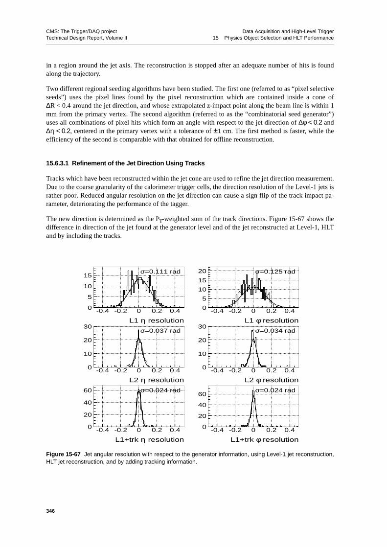
CMS: The Trigger/DAQ project Data Acquisition and High-Level TriggerTechnical Design Report, Volume II 15 Physics Object Selection and HLT Performance
in a region around the jet axis. The reconstruction is stopped after an adequate number of hits is foundalong the trajectory.
Two different regional seeding algorithms have been studied. The first one (referred to as “pixel selectiveseeds”) uses the pixel lines found by the pixel reconstruction which are contained inside a cone of∆R < 0.4 around the jet direction, and whose extrapolated z-impact point along the beam line is within 1mm from the primary vertex. The second algorithm (referred to as the “combinatorial seed generator”)uses all combinations of pixel hits which form an angle with respect to the jet direction of ∆φ < 0.2 and∆η < 0.2, centered in the primary vertex with a tolerance of ±1 cm. The first method is faster, while theefficiency of the second is comparable with that obtained for offline reconstruction.
15.6.3.1 Refinement of the Jet Direction Using Tracks
Tracks which have been reconstructed within the jet cone are used to refine the jet direction measurement.Due to the coarse granularity of the calorimeter trigger cells, the direction resolution of the Level-1 jets israther poor. Reduced angular resolution on the jet direction can cause a sign flip of the track impact pa-rameter, deteriorating the performance of the tagger.
The new direction is determined as the PT-weighted sum of the track directions. Figure 15-67 shows thedifference in direction of the jet found at the generator level and of the jet reconstructed at Level-1, HLTand by including the tracks.
Figure 15-67 Jet angular resolution with respect to the generator information, using Level-1 jet reconstruction,HLT jet reconstruction, and by adding tracking information.
0
5
10
15
-0.4 -0.2 0 0.2 0.4
L1 η resolution
0
5
10
15
20
-0.4 -0.2 0 0.2 0.4
L1 φ resolution
0
10
20
30
-0.4 -0.2 0 0.2 0.4
L2 η resolution
0
10
20
30
-0.4 -0.2 0 0.2 0.4
L2 φ resolution
0
20
40
60
-0.4 -0.2 0 0.2 0.4
L1+trk η resolution
0
20
40
60
-0.4 -0.2 0 0.2 0.4
L1+trk φ resolution
σ=0.111 rad σ=0.125 rad
σ=0.037 rad σ=0.034 rad
σ=0.024 rad σ=0.024 rad
346
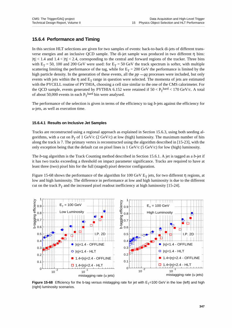
CMS: The Trigger/DAQ project Data Acquisition and High-Level TriggerTechnical Design Report, Volume II 15 Physics Object Selection and HLT Performance
15.6.4 Performance and Timing
In this section HLT selections are given for two samples of events: back-to-back di-jets of different trans-verse energies and an inclusive QCD sample. The di-jet sample was produced in two different η bins:|η| < 1.4 and 1.4 < |η| < 2.4, corresponding to the central and forward regions of the tracker. Three binswith ET = 50, 100 and 200 GeV were used: for ET = 50 GeV the track spectrum is softer, with multiplescattering limiting the performance of the tag, while for ET = 200 GeV the performance is limited by thehigh particle density. In the generation of these events, all the pp→qq processes were included, but onlyevents with jets within the η and ET range in question were selected. The momenta of jets are estimatedwith the PYCELL routine of PYTHIA, choosing a cell size similar to the one of the CMS calorimeter. Forthe QCD sample, events generated by PYTHIA 6.152 were retained if 50 < PT
hard < 170 GeV/c. A totalof about 50,000 events in each PT
hard bin were analysed.
The performance of the selection is given in terms of the efficiency to tag b-jets against the efficiency foru-jets, as well as execution time.
15.6.4.1 Results on Inclusive Jet Samples
Tracks are reconstructed using a regional approach as explained in Section 15.6.3, using both seeding al-gorithms, with a cut on PT of 1 GeV/c (2 GeV/c) at low (high) luminosity. The maximum number of hitsalong the track is 7. The primary vertex is reconstructed using the algorithm described in [15-23], with theonly exception being that the default cut on pixel lines is 1 GeV/c (5 GeV/c) for low (high) luminosity.
The b-tag algorithm is the Track Counting method described in Section 15.6.1. A jet is tagged as a b-jet ifit has two tracks exceeding a threshold on impact parameter significance. Tracks are required to have atleast three (two) pixel hits for the full (staged) pixel detector configuration.
Figure 15-68 shows the performance of the algorithm for 100 GeV ET jets, for two different η regions, atlow and high luminosity. The difference in performance at low and high luminosity is due to the differentcut on the track PT and the increased pixel readout inefficiency at high luminosity [15-24].
Figure 15-68 Efficiency for the b-tag versus mistagging rate for jet with ET=100 GeV in the low (left) and high(right) luminosity scenarios.
0
0.1
0.2
0.3
0.4
0.5
0.6
0.7
0.8
0.9
1
10-2
10-1
|η|<1.4 - OFFLINE
|η|<1.4 - HLT
1.4<|η|<2.4 - OFFLINE
1.4<|η|<2.4 - HLT
I.P. 2D
ET = 100 GeV
Low Luminosity
mistagging rate (u jets)
b-ta
ggin
g ef
ficie
ncy
0
0.1
0.2
0.3
0.4
0.5
0.6
0.7
0.8
0.9
1
10-2
10-1
|η|<1.4 - OFFLINE
|η|<1.4 - HLT
1.4<|η|<2.4 - OFFLINE
1.4<|η|<2.4 - HLT
I.P. 2D
ET = 100 GeV
High Luminosity
mistagging rate (u jets)
b-ta
ggin
g ef
ficie
ncy
347

CMS: The Trigger/DAQ project Data Acquisition and High-Level TriggerTechnical Design Report, Volume II 15 Physics Object Selection and HLT Performance
The performance is also compared with the one which could be obtained by using fully reconstructedtracks. No degradation is visible, so the online selection does not result in a reduced performance. A com-parison of the performance with the staged and full pixel detector is shown in Figure 15-69.
Figure 15-70 (left plot) compares the performance for the different bins of jet ET. The higher performanceof the tagging algorithm for 100 GeV ET jets is due to the reduction of the multiple scattering componentof the impact parameter error. On the othe hand, the 200 GeV jets have higher mistagging rate due to theincreased track multiplicity, while those at 50 GeV are limited by multiple scattering. A better perform-ance can be achieved using a three-dimensional impact parameter, as seen by comparing the performancefor the 100 GeV ET jets, also shown in Figure 15-70.
Figure 15-69 b-tag performance: comparison of the staged and full pixel detector configurations.
Figure 15-70 Efficiency for b-tagging versus the mistagging rate for different jet energies (left) and for 3D vs 2Dimpact parameters (right).
0
0.1
0.2
0.3
0.4
0.5
0.6
0.7
0.8
0.9
1
10-2
10-1
|η|<1.4
|η|<1.4 - STAGED
1.4<|η|<2.4
1.4<|η|<2.4 - STAGED
I.P.2D/HLT
ET = 100 GeV
Low Luminosity
mistagging rate (u jets)
b-ta
ggin
g ef
ficie
ncy
0
0.1
0.2
0.3
0.4
0.5
0.6
0.7
0.8
0.9
1
10-2
10-1
|η|<1.4 - 2D
|η|<1.4 - 3D
1.4<|η|<2.4 - 2D
1.4<|η|<2.4 - 3D
HLT
ET = 100 GeV
Low Luminosity
mistagging rate (u jets)
b-ta
ggin
g ef
ficie
ncy
0
0.1
0.2
0.3
0.4
0.5
0.6
0.7
0.8
0.9
1
10-2
10-1
ET = 50 GeV
ET = 100 GeV
ET = 200 GeV
I.P.2D/HLT
|η|<2.4
Low Luminosity
mistagging rate (u jets)
b-ta
ggin
g ef
ficie
ncy
348
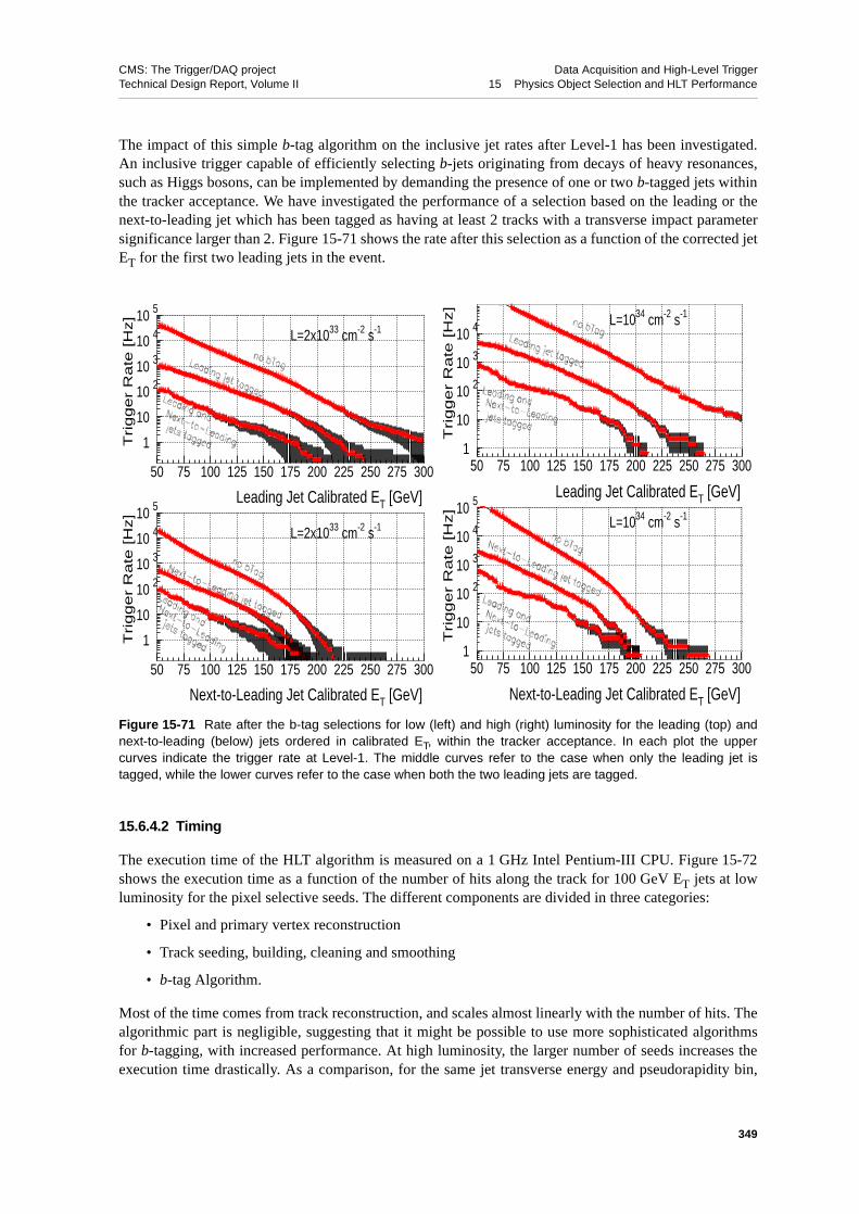
CMS: The Trigger/DAQ project Data Acquisition and High-Level TriggerTechnical Design Report, Volume II 15 Physics Object Selection and HLT Performance
The impact of this simple b-tag algorithm on the inclusive jet rates after Level-1 has been investigated.An inclusive trigger capable of efficiently selecting b-jets originating from decays of heavy resonances,such as Higgs bosons, can be implemented by demanding the presence of one or two b-tagged jets withinthe tracker acceptance. We have investigated the performance of a selection based on the leading or thenext-to-leading jet which has been tagged as having at least 2 tracks with a transverse impact parametersignificance larger than 2. Figure 15-71 shows the rate after this selection as a function of the corrected jetET for the first two leading jets in the event.
15.6.4.2 Timing
The execution time of the HLT algorithm is measured on a 1 GHz Intel Pentium-III CPU. Figure 15-72shows the execution time as a function of the number of hits along the track for 100 GeV ET jets at lowluminosity for the pixel selective seeds. The different components are divided in three categories:
• Pixel and primary vertex reconstruction
• Track seeding, building, cleaning and smoothing
• b-tag Algorithm.
Most of the time comes from track reconstruction, and scales almost linearly with the number of hits. Thealgorithmic part is negligible, suggesting that it might be possible to use more sophisticated algorithmsfor b-tagging, with increased performance. At high luminosity, the larger number of seeds increases theexecution time drastically. As a comparison, for the same jet transverse energy and pseudorapidity bin,
Figure 15-71 Rate after the b-tag selections for low (left) and high (right) luminosity for the leading (top) andnext-to-leading (below) jets ordered in calibrated ET, within the tracker acceptance. In each plot the uppercurves indicate the trigger rate at Level-1. The middle curves refer to the case when only the leading jet istagged, while the lower curves refer to the case when both the two leading jets are tagged.
Leading Jet Calibrated ET [GeV]
Trigg
er
Rate
[H
z]
L=2x1033 cm-2 s-1
Next-to-Leading Jet Calibrated ET [GeV]
Trigge
r R
ate
[H
z]
L=2x1033 cm-2 s-1
1
10
10 210 310 410 5
50 75 100 125 150 175 200 225 250 275 300
1
10
10 210 310 410 5
50 75 100 125 150 175 200 225 250 275 300
Leading Jet Calibrated ET [GeV]
Trigger
Rate
[H
z]
L=1034 cm-2 s-1
Next-to-Leading Jet Calibrated ET [GeV]
Trig
ge
r R
ate
[H
z]
L=1034 cm-2 s-1
1
10
10 2
10 3
10 4
50 75 100 125 150 175 200 225 250 275 300
1
10
10 2
10 3
10 4
10 5
50 75 100 125 150 175 200 225 250 275 300
349
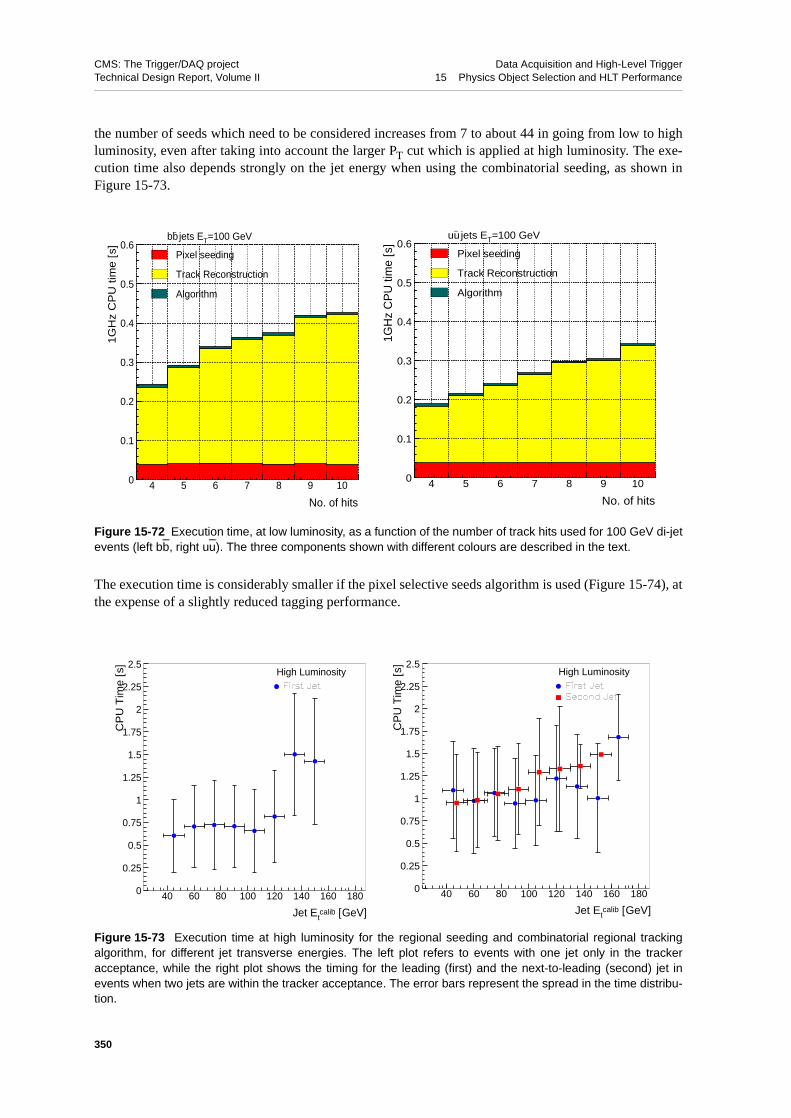
CMS: The Trigger/DAQ project Data Acquisition and High-Level TriggerTechnical Design Report, Volume II 15 Physics Object Selection and HLT Performance
the number of seeds which need to be considered increases from 7 to about 44 in going from low to highluminosity, even after taking into account the larger PT cut which is applied at high luminosity. The exe-cution time also depends strongly on the jet energy when using the combinatorial seeding, as shown inFigure 15-73.
The execution time is considerably smaller if the pixel selective seeds algorithm is used (Figure 15-74), atthe expense of a slightly reduced tagging performance.
Figure 15-72 Execution time, at low luminosity, as a function of the number of track hits used for 100 GeV di-jetevents (left bb, right uu). The three components shown with different colours are described in the text.
Figure 15-73 Execution time at high luminosity for the regional seeding and combinatorial regional trackingalgorithm, for different jet transverse energies. The left plot refers to events with one jet only in the trackeracceptance, while the right plot shows the timing for the leading (first) and the next-to-leading (second) jet inevents when two jets are within the tracker acceptance. The error bars represent the spread in the time distribu-tion.
No. of hits
1G
Hz
CP
U tim
e [s
]
bb − jets ET=100 GeV
Pixel seeding
Track Reconstruction
Algorithm
0
0.1
0.2
0.3
0.4
0.5
0.6
4 5 6 7 8 9 10
No. of hits
1GH
z C
PU
tim
e [s
]
uu − jets ET=100 GeV
Pixel seeding
Track Reconstruction
Algorithm
0
0.1
0.2
0.3
0.4
0.5
0.6
4 5 6 7 8 9 10
Jet Etcalib [GeV]
CP
U T
ime
[s]
High Luminosity
0
0.25
0.5
0.75
1
1.25
1.5
1.75
2
2.25
2.5
40 60 80 100 120 140 160 180
Jet Etcalib [GeV]
CP
U T
ime
[s]
High Luminosity
0
0.25
0.5
0.75
1
1.25
1.5
1.75
2
2.25
2.5
40 60 80 100 120 140 160 180
350

CMS: The Trigger/DAQ project Data Acquisition and High-Level TriggerTechnical Design Report, Volume II 15 Physics Object Selection and HLT Performance
15.6.5 Summary
The High-Level Trigger can benefit from efficient b-jet tagging at both low and high luminosity, with ex-ecution times which can be sustained in the processor farm running just after Level-1. Comparison withoffline tagging performance shows that no information is lost in this online tagging.
A possible dedicated b-tagged HLT stream with at least one jet inside the tracker acceptance and a b-tagbased on 2D impact parameter significance, S, might have the following cut parameters:
• For jets ET < 80 GeV: 2 tracks with S > 1.5;
• For jets 80 < ET < 150 GeV: 2 tracks with S > 2.0;
• For jets ET > 150 GeV: 2 tracks with S > 2.5.
Such a selection would allow to have about a 55% efficiency for b-jets and a rejection factor of about 10,almost independent of the jet ET. It would correspond to a rate of 5 Hz for a cut on the leading jet ET ofabout 200 GeV or 160 GeV on the next-to-leading jet.
This selection could be used in the case of SUSY searches, where the number of b-jets in the final statecan be large. In particular it would help in the HLT selection of point 6 and 6R (Section 15.8.3.2) and alsoin the cascade decays of χ2→χ1h→bb [15-25].
Figure 15-74 Execution time at high luminosity for the pixel lines algorithm, for different jet transverse energies.The first plot refers to events with one jet only in the tracker acceptance, while the plot on the right shows thetiming for the leading (first) and the next-to-leading (second) jet in events when two jets are within the trackeracceptance. The error bars represent the spread in the time distribution.
Jet Etcalib [GeV]
CP
U T
ime
[s]
High Luminosity
0
0.2
0.4
0.6
0.8
1
1.2
1.4
40 60 80 100 120 140 160 180
Jet Etcalib [GeV]
CP
U T
ime
[s]
High Luminosity
0
0.2
0.4
0.6
0.8
1
1.2
1.4
40 60 80 100 120 140 160 180
351

CMS: The Trigger/DAQ project Data Acquisition and High-Level TriggerTechnical Design Report, Volume II 15 Physics Object Selection and HLT Performance
15.7 Calibration and Monitor Samples
15.7.1 Calibration Methods and Samples
15.7.1.1 Tracker Alignment
The first task after the installation of the CMS tracker will be to precisely align all its components in a sin-gle reference frame. The intrinsic detector resolution can reach, for the pixels, a value as low as 10 µm.The alignment procedure should assure a level of precision such that the remaining error can be consid-ered negligible with respect to these figures.
It has been shown, in a simple test beam configuration, that the tracker can “autoalign” to the level of aµm, using charged tracks [15-26] and minimizing the track residuals in an iterative procedure. With thisprecision the aligned tracker performs as a perfectly aligned tracker. A limitation of this method is thattracking must be possible for the iteration to be started; if no tracks are found, there is no quantity that canbe minimized. To investigate this limitation numerous studies have been performed to check the track re-construction efficiency and the rate of fake tracks for large misalignments.
An ideal tracker alignment is simulated in CMSIM. Misalignment is simulated in the reconstruction,where misalignments can be introduced at four different levels, namely at the sub-detector level, at thelayer level, at the ring level and at the detector level. The elements at each of these levels can be rotated ortranslated independently, and the resulting overall alignment is a combination of the misalignments of thevarious components. The strategy chosen for track-finding in situations of large misalignment is to en-large the errors assigned to the reconstructed hits, so that the Kalman filter is still able to match the correcthits to be attached to a track. Naturally, this also results in a larger number of fake tracks being recon-structed, but the redundancy of the tracker layout is enough to maintain this rate at a reasonable level.
Figure 15-75 shows the tracking efficiency for muons from W→µν as a function of η. The rods and thewedges in the tracker silicon barrel layers are randomly misaligned up to 1 mm. When the reconstructionerror is enlarged to take into account the misalignment, no degradation in the efficiency is found. On the
Figure 15-75 Tracking efficiency (left), and fake rate (right) for W → µν events at low luminosity, for misalign-ments up to 1 mm.
352
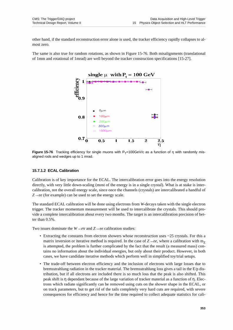
CMS: The Trigger/DAQ project Data Acquisition and High-Level TriggerTechnical Design Report, Volume II 15 Physics Object Selection and HLT Performance
other hand, if the standard reconstruction error alone is used, the tracker efficiency rapidly collapses to al-most zero.
The same is also true for random rotations, as shown in Figure 15-76. Both misalignments (translationalof 1mm and rotational of 1mrad) are well beyond the tracker construction specifications [15-27].
15.7.1.2 ECAL Calibration
Calibration is of key importance for the ECAL. The intercalibration error goes into the energy resolutiondirectly, with very little down-scaling (most of the energy is in a single crystal). What is at stake is inter-calibration, not the overall energy scale, since once the channels (crystals) are intercalibrated a handful ofZ→ee (for example) can be used to set the energy scale.
The standard ECAL calibration will be done using electrons from W-decays taken with the single electrontrigger. The tracker momentum measurement will be used to intercalibrate the crystals. This should pro-vide a complete intercalibration about every two months. The target is an intercalibration precision of bet-ter than 0.5%.
Two issues dominate the W→eν and Z→ee calibration studies:
• Extracting the constants from electron showers whose reconstruction uses ~25 crystals. For this amatrix inversion or iterative method is required. In the case of Z→ee, where a calibration with mZis attempted, the problem is further complicated by the fact that the result (a measured mass) con-tains no information about the individual energies, but only about their product. However, in bothcases, we have candidate iterative methods which perform well in simplified toy/trial setups.
• The trade-off between electron efficiency and the inclusion of electrons with large losses due tobremsstrahlung radiation in the tracker material. The bremsstrahlung loss gives a tail in the E/p dis-tribution, but if all electrons are included there is so much loss that the peak is also shifted. Thispeak shift is η dependant because of the large variation of tracker material as a function of η. Elec-trons which radiate significantly can be removed using cuts on the shower shape in the ECAL, oron track parameters, but to get rid of the tails completely very hard cuts are required, with severeconsequences for efficiency and hence for the time required to collect adequate statistics for cali-
Figure 15-76 Tracking efficiency for single muons with PT=100GeV/c as a function of η with randomly mis-aligned rods and wedges up to 1 mrad.
353

CMS: The Trigger/DAQ project Data Acquisition and High-Level TriggerTechnical Design Report, Volume II 15 Physics Object Selection and HLT Performance
bration. This leads to the strategy (for W→eν) of intercalibating individual crystals within a smallregion (in which the variation of tracker material is small) using loose cuts; and then intercalibrat-ing these small regions with much tighter cuts.
Short-term changes in crystal transparency due to radiation damage and recovery will be continuouslymonitored using the ECAL laser monitoring system. Light transported to the crystals through optical fi-bres, is injected, and the resulting signal pulses read out, during the ‘abort gaps’ in the LHC bunch struc-ture. The changes in crystal transparency occur rapidly (~hours) and saturate at a level dependant uponthe dose rate. In the absence of radiation there is a recovery which takes place with a time constant of sev-eral days. The magnitude of the changes in transparency expected depends on dose rate. In the barrel, atlow luminosity, the full extent of the damage should be less than 1%. At |η| = 2.5 it will be about 5%. Athigh luminosity the corresponding figures are expected to be 5% and 15%.
The laser system will also be used to transport the test beam ‘pre-calibration’ of a significant number ofsuper-modules (~10) and one endcap Dee to the experiment. The target is a transported intercalibrationprecision of better than 2% for those units which are exposed to the beam.
In addition to these standard tools, two others have been studied. Rings of crystals at fixed η can be inter-calibrated by imposing φ-symmetry on the recorded energy in them. By taking a dedicated stream of spe-cial triggers at high rate (~1kHz) and, in the HLT farm, stripping out the handful of crystals in each eventhaving energy above some threshold, an intercalibration at the level of ~2% can be obtained very rapidly.This has been investigated in detail for minimum-bias crossings [15-28], and is now being studied for thecase of high ET single jet triggers. The use of jet triggers would enable the calibration to be done withmuch larger energy deposits than are used with minimum-bias crossings. But work needs to be done inthis case to avoid any trigger bias. The φ-symmetry technique may be of particular importance at start-up,in order to rapidly achieve an acceptable intercalibration which yet falls short of the ultimate precisionaimed for. The rings in φ would have to be intercalibrated using another method. For this purpose, use ofZ-decays to two electrons is being studied. These events would come through the standard two electrontrigger. Preliminary results suggest that the φ-rings could be intercalibrated in a few days using Z-decays,even without the use of track information.
15.7.1.3 Calibration Samples for the HCAL
The HCAL has five distinct and complementary systems for calibration and monitoring [15-29]:
1. megatile scanner: a collimated gamma source to measure light yield of each tile of every megatile,
2. moving wire source, with gamma source tube(s) installed in every megatile that cross every tile
3. light injection: UV laser and blue-LED light injection into the readout box containing the HPDs,
4. test-beam calibration: four individual wedges with muons, electrons and hadrons are calibratedagainst the moving wire source for absolute energy calibration scale,
5. physics events in the CMS detector including jets and muons.
The megatile scanner is used to measure the relative light yield of each tile to better than 1% during theconstruction of the megatiles. The moving wire source will track the changes of each tile to better than0.7% throughout the life of the HCAL. In the readout box, UV laser and blue LED light will be used forthe timing of individual towers and for the measurement of the linearity of the readout electronics. The ra-dioactive source will transfer an absolute calibration, obtained with test beams of single-hadrons, to thecalorimeter. Test-beam and physics events will provide the ultimate jet energy calibration.
354
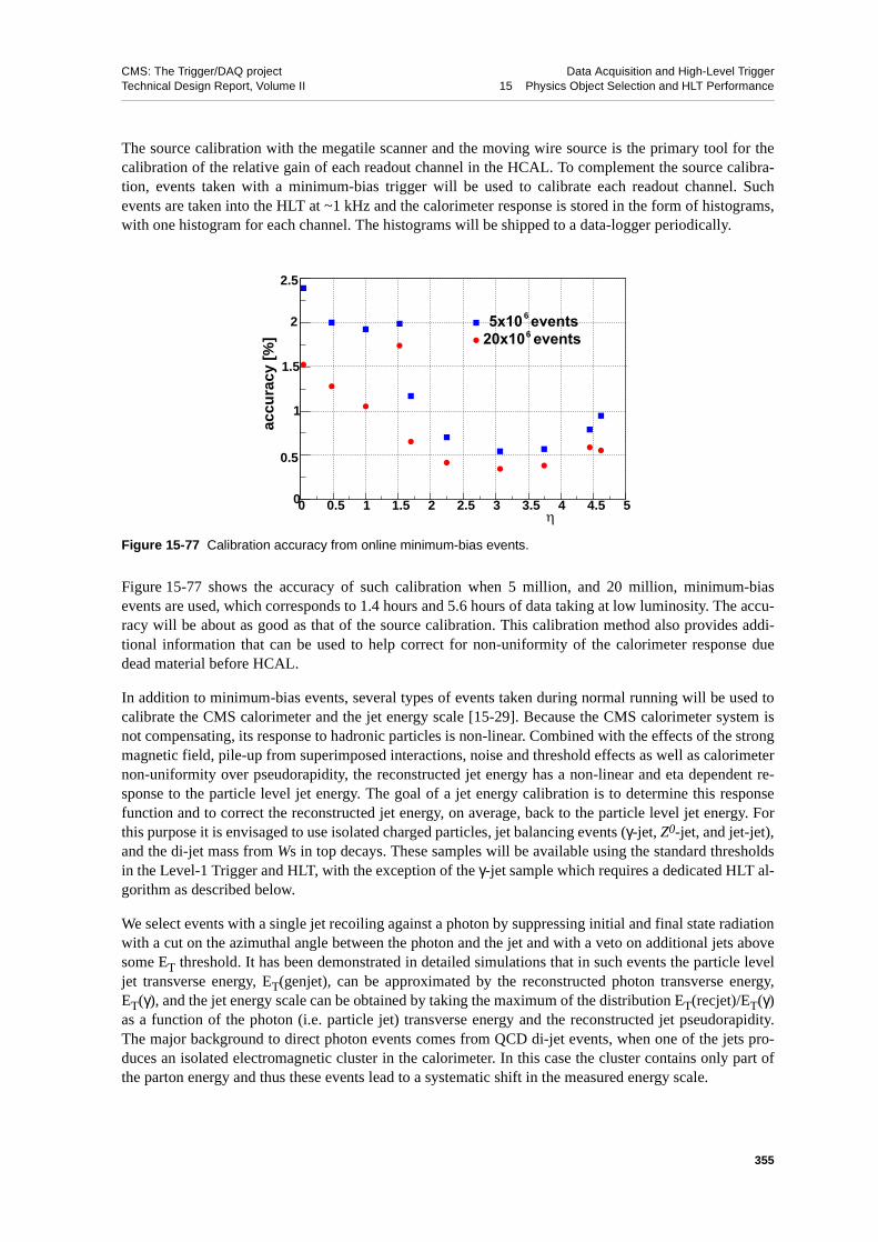
CMS: The Trigger/DAQ project Data Acquisition and High-Level TriggerTechnical Design Report, Volume II 15 Physics Object Selection and HLT Performance
The source calibration with the megatile scanner and the moving wire source is the primary tool for thecalibration of the relative gain of each readout channel in the HCAL. To complement the source calibra-tion, events taken with a minimum-bias trigger will be used to calibrate each readout channel. Suchevents are taken into the HLT at ~1 kHz and the calorimeter response is stored in the form of histograms,with one histogram for each channel. The histograms will be shipped to a data-logger periodically.
Figure 15-77 shows the accuracy of such calibration when 5 million, and 20 million, minimum-biasevents are used, which corresponds to 1.4 hours and 5.6 hours of data taking at low luminosity. The accu-racy will be about as good as that of the source calibration. This calibration method also provides addi-tional information that can be used to help correct for non-uniformity of the calorimeter response duedead material before HCAL.
In addition to minimum-bias events, several types of events taken during normal running will be used tocalibrate the CMS calorimeter and the jet energy scale [15-29]. Because the CMS calorimeter system isnot compensating, its response to hadronic particles is non-linear. Combined with the effects of the strongmagnetic field, pile-up from superimposed interactions, noise and threshold effects as well as calorimeternon-uniformity over pseudorapidity, the reconstructed jet energy has a non-linear and eta dependent re-sponse to the particle level jet energy. The goal of a jet energy calibration is to determine this responsefunction and to correct the reconstructed jet energy, on average, back to the particle level jet energy. Forthis purpose it is envisaged to use isolated charged particles, jet balancing events (γ-jet, Z0-jet, and jet-jet),and the di-jet mass from Ws in top decays. These samples will be available using the standard thresholdsin the Level-1 Trigger and HLT, with the exception of the γ-jet sample which requires a dedicated HLT al-gorithm as described below.
We select events with a single jet recoiling against a photon by suppressing initial and final state radiationwith a cut on the azimuthal angle between the photon and the jet and with a veto on additional jets abovesome ET threshold. It has been demonstrated in detailed simulations that in such events the particle leveljet transverse energy, ET(genjet), can be approximated by the reconstructed photon transverse energy,ET(γ), and the jet energy scale can be obtained by taking the maximum of the distribution ET(recjet)/ET(γ)as a function of the photon (i.e. particle jet) transverse energy and the reconstructed jet pseudorapidity.The major background to direct photon events comes from QCD di-jet events, when one of the jets pro-duces an isolated electromagnetic cluster in the calorimeter. In this case the cluster contains only part ofthe parton energy and thus these events lead to a systematic shift in the measured energy scale.
Figure 15-77 Calibration accuracy from online minimum-bias events.
0 0.5 1 1.5 2 2.5 3 3.5 4 4.5 5
accu
racy
[%
]
0
0.5
1
1.5
2
2.5
5x10 events20x10 events
6
6
η
355

CMS: The Trigger/DAQ project Data Acquisition and High-Level TriggerTechnical Design Report, Volume II 15 Physics Object Selection and HLT Performance
Since the CMS single photon HLT selection envisages storing only events with ET(γ) > 80 GeV, we needa dedicated calibration selection for lower energies. The production cross section of photon+jet events islarge. Making strong requirements at the trigger level on the event selection has a large advantage oversimple rate prescaling because the number of signal events contained in the sample eventually usable forthe offline analysis is larger. We expect a 60 Hz rate of single isolated electron-photons with ET(γ) >30GeV from signal events even after strong event selection cuts with low signal efficiency but with veryhigh background rejection.
The calibration trigger will select isolated HLT photon candidates and will then apply additional isolationcuts. Offline, we will make various selections, based on an azimuthal angle cut and veto on additionaljets, as part of our systematic studies. In what follows, we assume the efficiency of the final offline selec-tions is not less than 50%. Our current analysis uses the following photon isolation cuts for the calibrationtrigger at low luminosity: the transverse energy reconstructed in ECAL between cones 0.07 and 0.5around the photon candidate passes
where only crystals with ET >0.1 GeV are used, and no pixel line from the signal vertex is allowed in acone of radius 0.7 around the direction of the photon candidate. The signal vertex is reconstructed in thepixel detector as the vertex with a highest sum of pixel line transverse momenta. With these cuts we stillexpect total event rate of 25 Hz for ET(γ)>20 GeV which will be prescaled to a value consistent with theoverall resources for output to storage. Figure 15-78 shows the estimated number of events versus the ETof the photon after 3 months (2.5×10⁶ s) of low luminosity data taking assuming a 1 Hz trigger rate isavailable for calibration. The energy dependence of the prescale was set so that the statistical error on thecalibration was approximately constant over the range 20 GeV < ET(jet) < 100 GeV. With this prescale,we achieve a statistical error of less than 1% for the jets calibrated on the prescaled trigger. For jets thatare calibrated with the unprescaled trigger (ET(γ) > 80 GeV) the uncertainty will be smaller. Although the
Figure 15-78 Number of calibration events versusphoton ET (the bins have a width approximately equalto 10% of the photon ET) after 3 month low luminositydata taking for three jet pseudorapidity regions as afunction of ET(γ) threshold. A prescaled dedicated cali-bration trigger below 100 GeV and the single isolatedγ trigger above 100 GeV are used.
Figure 15-79 Statistical errors on the jet energy scalecalibration assuming the fit is done using bins with awidth approximately equal to 10% of the jet ET after 3month low luminosity data.
ηjet< 1.5
1.5 < ηjet< 3
3 < ηjet< 5
no.e
vent
s/bi
n
L int = 5 fb-1
10 2
10 3
10 4
10 5
10 6
102 103ET (GeV)
ηjet< 1.51.5 < ηjet< 33 < ηjet< 5
L int = 5 fb-1
ET (GeV)
calib
ratio
n ac
cura
cy (%
)
10-2
10-1
1
102 103
ET 0.005ET1.5 γ( )<
0.07 ∆R 0.5<<
∑
356

CMS: The Trigger/DAQ project Data Acquisition and High-Level TriggerTechnical Design Report, Volume II 15 Physics Object Selection and HLT Performance
unprescaled single photon trigger starts at 80 GeV, for demonstration purposes we assumed a fully effi-cient trigger only above ET(γ) > 100 GeV. The estimated statistical errors on the energy scale measured in10% wide ET(γ) bins are plotted in Figure 15-79. The calibration trigger can be implemented on top of theisolated photon HLT trigger, as a prescaled extension of the latter down to ET(γ) = 20 GeV.
15.7.1.4 Muon Calibration and Alignment
15.7.1.4.1 Calibration
The front-end electronics of the three muon systems (DT, CSC, and RPC) must be pulsed periodically inorder to find dead channels, scan and adjust discriminator thresholds, perform t0 measurements (DT),measure timing windows (RPC), measure charge to ADC-count conversion and linearity (CSC), andmeasure cross-talk (CSC). Additionally, test patterns will be injected in order to test the Level-1 Triggerlogic of all three systems. This pulsing can take place during periods without beams, or during the “abortgaps” in the LHC bunch structure. Additionally, noise measurements will be performed during periodswithout beam collisions in order to find noisy (high-rate) channels.
The calibrations are not expected to significantly add to the data volume generated during normal run-ning. For example, in pulsing the cathode front-end boards of the CSC system, the data volume per pulse(where a single channel of every front-end board is pulsed in parallel and all 96 channels of every boardare read out) is expected to be about 3.5 MB. A full CSC calibration is expected to take 10−20 minutesand generate approximately 300 GB of data.
15.7.1.4.2 Alignment
Misalignment of the muon chambers or the iron disks and wheels they are mounted on can change themeasured sagitta of a muon track, thus distorting the momentum measurement. To illustrate this effect,Figure 15-80a shows the effect of alternately rotating the barrel rings MB1−ΜΒ4 by ±0.5 mrad in φ (sim-ulating chamber positioning errors of 2−4 mm) on the muon Level-2 turn-on efficiency for a nominal PTthreshold of 40 GeV/c (defined at 90% of the plateau efficiency). The turn-on curve becomes noticeablyshallower than the curve for perfect alignment. The effect is smaller for lower thresholds, and the increaseof the Level-2 trigger rate from such misalignment is less than 5% for thresholds below about 40 GeV/c.The impact on the Level-3 PT measurement and turn-on efficiency from muon chamber misalignment isnegligible, however, as shown in Figure 15-80b, since the momentum measurement is dominated by thetracker measurements.
The alignment of the muon chambers is expected to be determined using an optical alignment system, asdiscussed in [15-30]. It is possible to perform an in situ alignment using high-PT collision muons [15-31],but uncertainty on the magnetic field in the yoke at the level of only 0.1% implies that it may take severalmonths of data collection at full luminosity to reach a precision of 200 µm, which is the position resolu-tion of a single measurement layer in the DT and CSC muon systems.
In the endcaps, it may be possible to use beam halo muons, travelling roughly parallel to the beam axis, toalign the chambers on the iron disks. The Global Level-1 Trigger will implement a dedicated trigger forsuch muons, which are identified by logic in the Level-1 CSC Track-Finder. Detailed studies still need tobe performed to determine the achieveable alignment precision.
357

CMS: The Trigger/DAQ project Data Acquisition and High-Level TriggerTechnical Design Report, Volume II 15 Physics Object Selection and HLT Performance
15.7.2 HLT Monitoring
A crucial aspect of the filtering process is the monitoring of the performance of the HLT and its properfunctioning. Both tasks can be achieved by analyzing online, and in some cases directing to storage,events that fail the HLT selection. For this purpose at least 1 Hz of events that have failed the HLT will bewritten to storage. These events will be analysed in near real-time, to identify rapidly any malfunctions inthe algorithms or the processors in the Filter Farm.
The online analysis will also be based on statistics accumulated by the HLT process in each Filter Unit.The latter will report key performance parameters, like the fraction of events accepted on each triggerpath, at regular intervals. Close monitoring of such quantities, as well as histogramming of select kine-matic quantities and topological properties of the objects selected, will be used to monitor the correctfunctioning of the HLT. More details on monitoring the Filter Farm and the High-Level Trigger can befound in Chapter 16, "Computing Services".
Figure 15-80 Efficiency for single muons to pass (a) the Level-2 and (b) the Level-3 muon trigger as a functionof the generated PT for a PT threshold of 40 GeV/c, with and without an alternating 0.5 mrad rotation of the bar-rel rings.
Generated µ PT(GeV)
Eff
icie
ncy
Muon Barrel rotations
perfect alignment
0.5 mrad misalignment
0
0.2
0.4
0.6
0.8
1
0 20 40 60 80 100Generated µ PT(GeV)
Eff
icie
ncy
Muon Barrel rotations
perfect alignment
0.5 mrad misalignment
0
0.2
0.4
0.6
0.8
1
0 20 40 60 80 100
(a) (b)
358

CMS: The Trigger/DAQ project Data Acquisition and High-Level TriggerTechnical Design Report, Volume II 15 Physics Object Selection and HLT Performance
15.8 HLT Performance
This section summarizes the physics object selection, the total estimate for the CPU requirements and thephysics performance of the HLT trigger table for the start-up luminosity of 2×1033 cm-2s-1.
15.8.1 Summary of HLT Selection
The current set of thresholds and rates to storage for each physics object, described in the preceding sec-tions, is listed in Table 15-24.
The values of the thresholds indicated in Table 15-24 are indicative of the type of event mixture that anoutput event rate of O(102) Hz would yield. The thresholds are optimized to guarantee high efficiency forgiven the maximum Level-1 Trigger rate and the are both observed. The latter is the subject of a follow-ing section.
15.8.2 CPU Requirement
A key issue for the High-Level Trigger selection is the CPU power required for the execution of the algo-rithms described thus far. The algorithms were timed, as described in the preceding sections, on a Pen-tium-III 1 GHz processor, and the current requirements vary from a very fast ~50 ms for jetreconstruction to the longer ~700 ms for muon reconstruction.
Table 15-24 High-Level Trigger requirements at low luminosity. The thresholds correspond to the values in ETor PT with 95% efficiency (90% efficiency for muons). There is no actual threshold in the HLT selection for τ-jets,so the threshold shown is that of the corresponding Level-1 Trigger requirement.
TriggerThreshold
(GeV or GeV/c)Rate (Hz)
Cumulative Rate (Hz)
Inclusive electron 29 33 33
Di-electrons 17 1 34
Inclusive photons 80 4 38
Di-photons 40, 25 5 43
Inclusive muon 19 25 68
Di-muons 7 4 72
Inclusive τ-jets 86 3 75
Di-τ-jets 59 1 76
1-jet * ETmiss 180 * 123 5 81
1-jet OR 3-jets OR 4-jets 657, 247, 113 9 89
Electron * Jet 19 * 45 2 90
Inclusive b-jets 237 5 95
Calibration and other events (10%) 10 105
TOTAL 105
359

CMS: The Trigger/DAQ project Data Acquisition and High-Level TriggerTechnical Design Report, Volume II 15 Physics Object Selection and HLT Performance
The first step is to weight the CPU needs of the algorithms by the frequency of their application, which isthe Level-1 Trigger rate of the corresponding channels. This is shown in Table 15-25 and yields a total of4092 CPU seconds as the total need to cover the 15.1 kHz of events allocated in the Level-1 Trigger ta-ble1. This translates to a mean of 271 ms per event that passes the Level-1 Trigger.
The second step is to translate this measurement to a standard measure of CPU power. To connect the cur-rent measurement to earlier estimates of the CPU requirements, the SpecInt95 (SI95) benchmarking unitwas chosen. The Pentium-III 1 GHz CPU capacity is estimated to be 41 SI95. Using these figures, the to-tal CPU power required to process the maximum Level-1 Trigger rate of 100 kHz by the HLT farm is1.2×106 SI95. This is the figure quoted in Chapter 2, “Overview”.
What is more relevant, however, is the estimate of the CPU power needed to carry out the physics pro-gram at the start-up of the LHC, when the luminosity will not have reached its full value. The current sce-nario for CMS is to have a DAQ system capable of reading a maximum of 50 kHz of events accepted bythe Level-1 Trigger. The CPU requirement for this system is thus one half of the total, i.e. 6×10⁵ SI95 or,in terms of CPU “units”, 15,000 CPUs as in those available in a standard commercial Personal Computer(PC).
The third and final step is the extrapolation of these figures to the year 2007. In this step a number of var-iables should be considered, including changes in the architecture of the basic microprocessors and mem-ory, as well as changes in the software itself. No such detailed analysis has been carried out, in the beliefthat the uncertainties are too large for such considerations to improve the reliability of the estimate. In-stead, the basic thesis of Moore’s Law, i.e. that CPU power increases by a factor two every 1.5 years, isused. Given the time period between now and the start of the first physics run, in 2007, there are threesuch 1.5 year periods, and thus the CPU units of 2007 should be a factor ~8 more powerful than those oftoday, thus requiring ~40ms per event. This implies that a total of ~2,000 CPUs are needed for the systemat the LHC start-up . This is the basis of the 1,000 dual-CPU PCs used in the cost estimates of Chapter 17.
There are, naturally, large uncertainties in the above estimate, listed in order of importance:
• A major uncertainty is related to all the samples that have not been simulated. Inherent in the aboveestimate is the assumption that all events in the 50 kHz of events accepted by the Level-1 Triggerwill require the full 300 ms. However, only 16 kHz of the total of 50 kHz has really been simulat-
Table 15-25 Summary of CPU time required for the selection of each physics objects in the HLT. The CPU fig-ures refer to a 1 GHz Intel Pentium-III CPU.
Physics ObjectCPU time per Level-1
event (ms)Level-1 Trigger rate
(kHz)Total CPU time
(s)
Electrons/photons 160 4.3 688
Muons 710 3.6 2556
Taus 130 3.0 390
Jets and ETmiss 50 3.4 170
Electron + Jet 165 0.8 132
B-jets 300 0.5 150
1. In the full Level-1 Trigger rate allocation of Table 15-1 there is an additional 0.9 kHz of minimum bias events thatwill be used for calibration and monitoring. These events are assumed to require the same amount of CPU as themean of the 15.1 kHz of events for which CPU time estimates are available.
360

CMS: The Trigger/DAQ project Data Acquisition and High-Level TriggerTechnical Design Report, Volume II 15 Physics Object Selection and HLT Performance
ed, with the rest of the events being included in the “safety factor” in the allocation of the Level-1Trigger bandwidth. It is clear that much of this safety factor will be used, since basic processesfrom the beam in the machine, e.g. beam halo, have not been included. It is expected, however, thatsuch processes will require far less CPU to identify and reject.
• The figure of ~300 ms per event accepted by the Level-1 Trigger does not include all the process-ing needed to go from the actual raw data to the final decision by the HLT. The overhead from thesoftware framework for accessing the DAQ packets of raw data, and the time needed to unpack theraw data in the form needed by the reconstruction algorithm are not included. These times cannotbe measured at present, since the raw data formats are not finalized. First estimates suggest that theCPU requirement can be significant, taking up to one quarter of the total reconstruction time.
• The selection of Table 15-24 is only an example of the type of requirements and rates involved inthe HLT selection, and the actual trigger table will very likely include additional selections. In par-ticular, it is expected that more selections involving combined objects will be introduced. This wilincrease the required CPU time.
• The time needed to process a single combination depends on the actual implementation of the re-construction algorithm and the underlying libraries, e.g. the mathematical and memory allocationones. It also depends on the quality of the compiler. In this respect also the current CPU time esti-mates are an upper limit. The current time estimates are dominated by the muon reconstructionstep which is in turn dominated by the GEANE extrapolation step. A significant speed-up is ex-pected when the extrapolation package is upgraded. Morever, the current package used for matrixalgebra will be replaced with a better one, while specialized memory allocators wil be used for cas-es where the memory management overhead has been measured to be significant. Such modifica-tions require little or no change to the reconstruction source code and can be done at a later stagewithout compromising algorithmic correctness.
• There are uncertainties arising from the actual occupancy in the CMS sub-detectors. The timeneeded to perform a given pattern recognition and/or reconstruction task depends on the number ofelements or combinations that need to be considered in order to reach a given reconstruction effi-ciency, as well as on the time needed to treat each element. The minimum number of combinationsneeded to achieve a given efficiency depends on the occupancy of the detectors, and on the accura-cy of each measurement. The occupancy, in turn, has uncertainties arising from the event genera-tors description of the hard interaction, the noise level in the detector, including the full readoutchain, the neutron background in the detector, and finally from beam backgrounds. The accuracyof each measurement has an uncertainty related to the current understanding of the detector and ac-curacy of the detector response simulation knowledge of the calibration and alignment at HLTtime. All these uncertainties have reasonable estimates or are expected to be sufficiently small tobe neglected in the present studies.
The CMS HLT reconstruction algorithms underwent rapid development in the context of the DAQ TDR,and this development will continue after the publication of the present document. The CPU time measure-ments given in this document reflect the current state of the algorithms. A reliable estimate of the CPUpower needed for the first physics run in 2007 is difficult to make. There are significant uncertainties inthe estimates, as explained above, and for this reason no attempt is made to estimate the potentialspeed-ups mentioned. Instead, such CPU savings are considered to be part of the “contingency” on CPU,to be used on all the processing steps that will require additional processing, as described above.
It is expected that the CMS reconstruction software will continue to evolve considerably between nowand the first physics run. The HLT filtering step should benefit from all improvements, since the codeused in the HLT, with the exception of the input and output mechanisms, is identical to the code to be usedoffline.
361

CMS: The Trigger/DAQ project Data Acquisition and High-Level TriggerTechnical Design Report, Volume II 15 Physics Object Selection and HLT Performance
15.8.3 Efficiency of HLT Selection for Major Physics Channels
15.8.3.1 Higgs Physics
The search for the Higgs boson is one of the most important tasks of experiments at the LHC. This sectionsummarizes the studies of the Higgs signals, described in Section 15.2 and in Section 15.3 for the Stand-ard Model (SM) Higgs and in Section 15.5 for some MSSM Higgs channels. Specific channels which in-volve peculiarities in the final state, e.g. an “invisible Higgs boson”, are discussed in other sections below.
The mass range to discover the Standard Model Higgs at the LHC ranges from the present negative searchlimit of LEP 114.4 GeV/c2 to approximately 1 TeV/c2. In the heavy mass range the channels with the bestsensitivity for Higgs masses up to 800 GeV/c2 is H→ZZ. In particular H→ZZ→µµµµ will be the“gold-plated” channel above MH=180 GeV/c2. For lower values of the Higgs mass the decay channelsH→WW(*)→llνν, qqH→qqWW(*), qqH→qqττ , ttH→ttγγ, ttH→ttbb, WH→Wγγ and H→γγ can also beused to discover and study the Higgs.
For the region around 120 GeV/c2 the most promising channels to date are the fusion processes or the de-cays into two photons. The decay H→γγ will be triggered at the HLT requiring two photons detected inthe ECAL and validated by the tracker, using the asymmetric cuts of ET > 40 and 25 GeV for the photons.This cut is equal to the proposed final offline selection for this channel. It yields a final background rate totape of 5 Hz. For low-luminosity running the combined Level-1/HLT trigger efficiency for a Higgs withmass of 115 GeV/c2, amounts to 77% for all those decays where both photons are within the ECAL fidu-cial volume |η| < 2.5. With respect to all events where the decay photons have the offline minimum ET,the efficiency is 83.7%. The geometrical acceptance for the two photons to be within the fiducial volumeis 65%. The trigger efficiency for high luminosity running is typically 5% lower.
The channel H→WW(*)→µµνν has been studied for Higgs mass values of 120, 160 and 200 GeV/c2. Thecombined low-luminosity HLT trigger consists of a single muon PT threshold of 19 GeV/c and a symmet-ric double muon threshold of 7 GeV/c and has a total output event rate of 29 Hz. The total efficiencywithin the fiducial acceptance is 92% at MH = 160 GeV/c2. The efficiency increases with increasingHiggs mass. The efficiency for this trigger reduces by 10-15% at high luminosity, because the thresholdshave to be increased to 31 and 10 GeV/c for the single and double muon trigger respectively.
The golden channel mentioned above H→ZZ→4µ has near-full efficiency since the efficiency for e.g.Z→µµ is about 92%. These efficiencies are relative to having at least one muon inside the geometric ac-ceptance of the trigger, |η| < 2.1, and all final state muons (two or four, depending on the channel) insidethe full acceptance of the muon system: |η| < 2.4.
These examples show that working HLT trigger schemes with good efficiency have been identified forSM Higgs particles, while in general, a heavy Standard-Model Higgs particle will be easier to trigger onthan a light one.
For MSSM neutral high-mass Higgs particles, A/H, and the charged Higgs the “golden” decays to heavygauge bosons are closed or strongly suppressed. Therefore alternative decay channels have been studied,in particular the decay modes A/H→ττ and H+→τ+ν. The main background to these channels are QCDjets. The τ-jets are identified as described in Section 15.5. The identification can be performed by calo-rimeter tau jet candidates supplemented either by a fast track finding algorithm in the pixel detectors or byusing regional reconstructed track finding algorithm. For the low luminosity runs the latter algorithm isfound to be more efficient, giving an efficiency of about 45% (49%) for MH = 200 GeV/c2
(MH = 500 GeV/c2), at the same time giving the required background reduction of a factor 1000. Both
362

CMS: The Trigger/DAQ project Data Acquisition and High-Level TriggerTechnical Design Report, Volume II 15 Physics Object Selection and HLT Performance
τ-jets are required to pass the trigger criteria. The corresponding efficiencies for high luminosity runningare about 15% lower.
A similar trigger can be devised for the charged heavy Higgs decay H+→τ+ν, requiring one τ-jet to beidentified and missing ET at the HLT. The efficiencies are 58% (MH = 200-400 GeV/c2) for the low-lumi-nosity runs and are about 10% lower at high luminosity.
For the neutral MSSM Higgs the combined electron/τ-jet trigger channels have been studied for the decayA/H→ττ→e+τ-jet. The combined trigger has a reduced threshold on the electron, compared to the sin-gle-electron trigger and has an HLT efficiency of 70% at both low and high luminosity. The overall effi-ciency of the combined trigger are only about 2-5% higher than those of the single electron trigger, butthis is mostly due to the choice of a relatively high mass for the Higgs. For Higgs masses around120 GeV/c2, the fusion channel qqH→qqττ benefits from such a trigger. Similar studies were made forthe channel A/H→ττ→µ+τ-jet and give an efficiency of 54% (46%) at low (high) luminosity.
15.8.3.2 Supersymmetry Searches
One of the main goals of the LHC is to look for evidence for Supersymmetry (SUSY), perhaps the mostpopular extension of the Standard Model. If SUSY exists, significant-sized samples of sparticle eventsshould be accumulated shortly after LHC turn-on. However, unless SUSY is discovered at the Tevatronbefore the LHC satrt-up, the signature of SUSY will not be known in advance.
The most popular SUSY models invoke the conservation of R-parity (RP), which makes the lightest Su-persymmetric particle, a neutral gaugino in most models, stable. In these models, squark and gluinoevents, which are produced strongly and therefore have very large production cross section, would appearin the detector as events with multiple jets and large ET
miss. More challenging from a trigger point of vieware models where the RP is not conserved and superparticles decay predominantly to jets. In some of thesemodels, the lightest neutral gaugino decays to three jets, and the signature of squark and gluino produc-tion could be a large number of jets. There can be some moderate ET
miss due to decays of top quarks, Wand Z-bosons, b-quarks and τ-leptons produced during the squark/gluino decays.
Supersymmetry models have a very large number of free parameters and thus a wide variety of possiblesignatures at the LHC. There have been several studies to find points in the SUSY parameter space thatwill in some way span the range of predictions that apply to the start of the LHC. Reference [15-32] wasused to select a few points to study for this TDR. These points all use the mSUGRA parameterization ofthe SUSY parameter space. Other parameterizations have not been considered, since the purpose of thisstudy is not to provide an exhaustive study of SUSY but only to provide examples of the type of Level-1and HLT requirements that are needed to provide good efficiency for SUSY events.
At low luminosity, the greatest challenge comes from the points with the lowest sparticle masses, justabove the reach of the Tevatron, because the transverse energies of the jets and ET
miss are smallest. Athigh luminosity, the challenge is to maximize the acceptance for the highest mass points, since they havethe smallest cross section.
Table 15-26 lists the parameters1, the masses of the sparticles and the cross sections for the points wehave studied for this TDR. The SUSY mass spectra and branching ratios were calculated using ISAWIG1.104 which uses ISAJET 7.51. This information was imported into HERWIG 6.301, which was used to
1. In the mSUGRA parameterization of the SUSY parameter space, m0 is the common scalar mass at the unificationscale, m1/2 is the common gaugino mass, A0 is the trilinear scalar coupling constant, β is the ratio of the vacuumexpectation value of the two Higgs doublets, and µ is the higgsinos mixing parameter.
363

CMS: The Trigger/DAQ project Data Acquisition and High-Level TriggerTechnical Design Report, Volume II 15 Physics Object Selection and HLT Performance
do the actual event generation. The points were chosen to give a variety of potential SUSY signatures.Point 41 has enhanced slepton (especially stau) production. Point 5 is a “typical” SUSY point withsquarks lighter than gluinos and therefore lots of ET
miss. Point 6 has gluinos lighter than squarks and thustends to have more jets and less ET
miss than a typical point. Point 7 has enhanced tau and sneutrino pro-duction. Point 8 is characterized by which yields an enhanced (b)-jet yield compared to Point 7,while the ET
miss is similar to that in Point 7. For point 9, the gluinos are lighter than all squarks, except forthe lighter stop, , thus allowing the decay which in fact dominates and therefore events havemany jets and smaller ET
miss. While these exact points (points 4, 5, and 6 in particular) may be excludedby LEP Higgs searches, Higgs production and the exact mass for the Higgs in the decays does not play animportant role in the observability or the characteristics of these events. The events were generated usingISAJET. The same points are used to simulate SUSY with R-parity violation with .
Table 15-26 Parameters used for the generation of the SUSY mSUGRA samples used in this TDR. The valuesA0 = 0, tanβ = 10, and µ > 0 were also used.
Point M0 M1/2 σ Mh
(GeV/c2) (GeV/c2) (pb) (GeV/c2) (GeV/c2) (GeV/c2) (GeV/c2)
4 20 190 181 466 410 70 110
5 150 180 213 447 415 66 110
6 300 150 500 349 406 45 106
7 250 1050 .017 2235 1986 445 122
8 900 930 .022 2032 1962 391 121
9 1500 700 .059 1625 1975 293 120
1. The labels given to the points (point 4, point 5, etc) are based on a historical convention with no significance here.
Figure 15-81 HLT rate vs. efficiency for SUSY signals, for events that pass the Level-1 jet+ETmiss Level-1 Trig-
ger. Left: the requirement is for four jets above a threshold which varies and leads to the contours shown, withone contour for each SUSY point. Right: the requirement is for one jet+ET
miss and ETmiss is varied.
m g( ) m uL( ) m χ10( )
χ2˜ hχ1
˜→
t1 g tt1→
χ1˜ 0
jjj→
1
10
10 2
10 3
0 0.1 0.2 0.3 0.4 0.5 0.6 0.7 0.8 0.9 1
6.8 Hz
SUSY Signal Efficiency
Rat
e (H
z)
● Point 4■ Point 5▲ Point 6
Point 4RPoint 5RPoint 6R
1
10
10 2
10 3
0 0.1 0.2 0.3 0.4 0.5 0.6 0.7 0.8 0.9 1
5.1 Hz
SUSY Signal Efficiency
Rat
e (H
z)
● Point 4■ Point 5▲ Point 6
Point 4RPoint 5RPoint 6R
364

CMS: The Trigger/DAQ project Data Acquisition and High-Level TriggerTechnical Design Report, Volume II 15 Physics Object Selection and HLT Performance
For the low-mass points, a few simple triggers with jets and ETmiss were considered. At low luminosity a
Table 15-27 The Level-1 and High-Level Trigger cut values, rates and efficiencies for six Supersymmetrypoints at low luminosity. The HLT efficiencies are with respect to events that pass the Level-1 Trigger. Allthresholds refer to the values with 95% efficiency, with the exception of the Level-1 ET
miss which is the actualcut value. For a definition of the SUSY points, see text.
Level-1 Trigger High-Level Trigger
SUSY point1 Jet >79 GeV+ET
miss>46 GeV 3 jets, ET>86 GeV1 Jet >180GeV+ET
miss>123 GeV 4 jets, ET>113 GeV
efficiency (%)
efficiency (%)(cumulative efficiency) efficiency (%)
efficiency (%)(cumulative efficiency)
4 88 60 (92) 67 11 (69)
5 87 64 (92) 65 14 (68)
6 71 68 (85) 37 16 (44)
4R 67 89 (94) 27 28 (46)
5R 58 90 (93) 17 30 (41)
6R 47 84 (87) 9 20 (26)
Background rate (kHz)rate (kHz)
(cumulative rate) rate (Hz)rate (Hz)
(cumulative rate)
2.3 0.98 (3.1) 5.1 Hz 6.8 (11.8)
Table 15-28 The Level-1 and High-Level Trigger cut values, rates and efficiencies for six Supersymmetrypoints at high luminosity. The HLT efficiencies are with respect to events that pass the Level-1 Trigger. Allthresholds refer to the values with 95% efficiency, with the exception of the Level-1 ET
miss which is the actualcut value. For a definition of the SUSY points, see text.
Level-1 Trigger High-Level Trigger
SUSY point1 Jet >113 GeV+ET
miss>70 GeV 3 jets, ET>111 GeV ETmiss>239 GeV 4 Jets, ET>185 GeV
efficiency (%)
efficiency (%) (cumulative efficiency) efficiency (%)
efficiency (%) (cumulative efficiency)
7 90 62 (90) 85 18 (85)
8 97 76 (98) 90 28 (92)
9 91 67 (94) 72 28 (76)
7R 91 99 (100) 70 75 (90)
8R 86 100 (100) 58 78 (88)
9R 75 99 (100) 41 52 (64)
Background rate (kHz)rate (kHz)
(cumulative rate) rate (Hz)rate (Hz)
(cumulative rate)
4.5 1.1 (5.4) 1.6 1.5(3.0)
365

CMS: The Trigger/DAQ project Data Acquisition and High-Level TriggerTechnical Design Report, Volume II 15 Physics Object Selection and HLT Performance
3-jet trigger and a jet+ETmiss trigger are considered at Level-1. For the HLT, a jet+ET
miss and a 4-jet chan-nel are considered. Figure 15-81(left) shows the 4-jet trigger rate versus efficiency for events that pass theLevel-1 Trigger jet+ET
miss criteria for the six SUSY points as the threshold on the jets is varied.Figure 15-81(right) shows the rate versus efficiency for the jet+ET
miss trigger as the threshold on the ET-miss is varied. The arrows on the plots show the thresholds chosen for the low luminosity trigger table asa compromise between efficiency and bandwidth. The cut values, trigger rates and signal efficiencies aregiven in Table 15-27. This simple table is sufficient for LHC turn-on. After the first few runs, and oncethe actual trigger conditions are known, more triggers will be added to increase the efficiency for SUSY
For the high luminosity case, the high mass SUSY points 7, 8, and 9 are considered. It is relatively easy todesign highly efficient triggers for these samples. Table 15-28 summarizes the optimized Level-1 andHLT requirements and output rates. The Level-1 Trigger has a single jet+ET
miss and a 3-jet trigger, whilethe HLT has an ET
miss and a 4-jet trigger. For these high mass points, it is easy to get a very efficient trig-ger table with only a few trigger terms, even for R-parity violating SUSY.
15.8.3.3 Invisible Higgs
Some extensions of the Standard Model (SM) contain Higgs bosons which can decay into stable neutralweakly interacting particles, therefore giving rise to “invisible” final states. In recent work[15-33][15-34], it was shown that the potential for discovering a Higgs boson decaying invisibly at theLHC can be extended considerably by studying Higgs production via weak boson fusion (WBF). Thepresence of the two forward-backward tagging jets that accompany Higgs production via weak boson fu-sion is a powerful tool for separating signal from the very large backgrounds. The large rapidity gap be-tween the two tagging jets is used in the trigger definition. The following offline cuts for an invisibleHiggs analysis were proposed in reference [15-33] and checked using a detailed simulation [15-34]:
1. ETj > 40 GeV, |ηj| < 5.0, |ηj1-ηj2| > 4.4, ηj1ηj2 < 0,
2. ETmiss > 100 GeV
3. Mjj > 1200 GeV/c2
4. ∆φjj < 1
The efficiencies of the Level-1 Trigger and the HLT selections discussed below are the efficiencies forevents that pass these offline selections.
The HF calorimeters play a crucial role in the selection of the invisible Higgs because of the two for-ward-backward tagging jets. The relative acceptance in the HF calorimeter (3.0<|η|<5.0) for these jets af-ter requiring ET>30 GeV for each jet is shown in Table 15-29 before and after the cut on the rapidity gapbetween the jets. After the rapidity gap constraint, almost 80% of the Higgs events will have at least onetagging jet in the HF.
The Level-1 jet trigger covers the entire calorimeter acceptance, including the HF calorimeter. At Level-1a jet+ET
miss trigger can therefore be used for the invisible Higgs selection. Figure 15-82 shows the trans-verse energy of the highest ET jet (left plot) and calorimeter ET
miss (right plot) reconstructed offline and at
Table 15-29 Acceptance of the CMS HF calorimeter to tagging jets (ET > 30 GeV) in the qq → qqH process.
no jets in HF one jet in HF 2 jets in HF
no cut on |ηj1-ηj2| 49% 45% 6%
|ηj1-ηj2|>4.4 22% 65% 13%
366

CMS: The Trigger/DAQ project Data Acquisition and High-Level TriggerTechnical Design Report, Volume II 15 Physics Object Selection and HLT Performance
Level-1 at L = 1034cm-2s-1 for Higgs events passing the WBF requirements and for a Higgs mass of120 GeV/c2 (which is slightly higher than the current limit of 114.4 GeV/c2 from LEP-II [15-35]). TheLevel-1 Trigger was optimized by examining the trigger rate for a single jet plus ET
miss trigger vs. the sig-nal efficiency by changing the ET
miss thresholds for the fixed set of single jet thresholds. Figure 15-83
shows the Level-1 jet+ETmiss trigger rate and Higgs efficiency for single jet thresholds of 70(60), 90(70),
110(80) at high (low) luminosity when the ETmiss threshold is varied.
Figure 15-82 Higgs events in the process qq → qqH, with the Higgs decaying invisibly, MH = 120 GeV/c2, andwhich pass the WBF cuts. Left plot: transverse energy of the highest-ET jet reconstructed in offline (solid histo-gram) and at Level-1 (dashed histogram). Right plot: ET
miss reconstructed offline (solid histogram) and atLevel-1 (dashed histogram). The luminosity is L=1034cm-2s-1.
Figure 15-83 QCD 2-jet rate (in kHz) for a jet+ETmiss trigger vs efficiency for qq → qqH, with the Higgs decay-
ing invisibly, for a Higgs mass of MH = 120 GeV/c2, and for events which passed WBF cuts when the ETmiss
threshold is varied and with single jet thresholds as labelled. Left (right) plot: low (high) luminosity.
0
10
20
30
40
50
60
70
80
90
100
0 50 100 150 200 250 300 350 400
ET jet at Level-1 and HLT, GeV
nev/
20 G
eV
qq→qqH, H(120 GeV)→inv
passed WBF selections
solid - 1st HLT jet
dotted - 2nd HLT jet
dashed - 1st Level-1 jet
L=1034cm-2s-1
0
10
20
30
40
50
60
70
80
0 50 100 150 200 250 300 350 400
ET miss at Level-1 and HLT, GeV
nev/
20 G
eV L=1034cm-2s-1
qq→qqH, H(120 GeV)→invpassed WBF selections
solid - HLT ET miss
dashed - Level-1 ET miss
0.7
0.75
0.8
0.85
0.9
0.95
1
10-2
10-1
1Level-1 Jet+MET Rate (kHz)
ε Leve
l-1 fo
r of
f-lin
e qq
H, H
→in
v (%
)
J > 60 GeV
J > 70 GeV
J > 80 GeV
MH=120 GeV
L=2x1033cm-2s-1
0.4
0.5
0.6
0.7
0.8
0.9
1
10-1
1 10Level-1 Jet+MET Rate (kHz)
ε Leve
l-1 fo
r of
f-lin
e qq
H, H
→in
v (%
)
J > 70 GeV
J > 90 GeV
J > 110 GeV
MH=120 GeV
L=1034cm-2s-1
367

CMS: The Trigger/DAQ project Data Acquisition and High-Level TriggerTechnical Design Report, Volume II 15 Physics Object Selection and HLT Performance
Table 15-30 lists the Level-1 1-jet+ETmiss trigger thresholds and the Higgs efficiency for Level-1
1-jet+ETmiss trigger rates of 0.2, 0.5 and 1.0 kHz at low and high luminosity. A rate of 0.5 kHz gives a
Higgs efficiency that is quite high: 98% (80%) for low (high) luminosity.
For the HLT selection, the first of the four sets of offline requirements listed earlier (the cuts on ET’s andη’s) are used along with the requirement Mjj > 1 TeV/c2, and a cut on ET
miss. The values for the cuts onET and |η| are the same as those for the offline. Figure 15-84 (left plot) displays the rate for QCD multi-jetevents as a function of the cutoff on ET
miss with only the first of the four sets of offline requirements ap-plied, and with the first and the Mjj cut applied. A rate of 0.1 Hz can be reached at low luminosity forET
miss >110 GeV without the Mjj cut. The signal efficiency in this case is near 100% since the offline cuton ET
miss is 100 GeV (see Figure 15-82). At high luminosity a rate of 0.2 Hz can be reached with the Mjjcut and an ~150 GeV threshold on ET
miss. The total Level-1 1-jet+ETmiss and HLT efficiency for Higgs at
high luminosity is shown in Figure 15-84 (right plot) as a function of the ETmiss cutoff. For 0.2 Hz rate
(ETmiss > 150 GeV and Mjj > 1 TeV/c2) the Higgs efficiency is 0.7.
Table 15-30 Summary of the single-jet plus ETmiss Level-1 Trigger thresholds for a total trigger rate of
0.2, 0.5, and 1.0 kHz at low and high luminosity. Shown are the jet and ETmiss thresholds, the efficiency
for qq → qqH with the Higgs (with MH = 120 GeV/c2) decaying invisibly for events which pass the WBFcuts.
Rate for Level-1 1-jet+ETmiss trigger 0.2 kHz 0.5 kHz 1.0 kHz
Low Luminosity single-jet threshold, ET
miss threshold (GeV)60,73
60,64
60,56
efficiency 0.96 0.98 0.99
High Luminosity single-jet threshold, ET
miss threshold (GeV)70,122
70,112
70,103
efficiency 0.72 0.79 0.84
Figure 15-84 Left plot: QCD 2-jet background rate after topological WBF cuts (1) as a function of the ETmiss cut-
off for L = 1034cm-2s-1 (solid histogram) and L = 1033cm-2s-1 (dashed histogram). Right plot: total Level-1 singlejet plus ET
miss rate and HLT efficiency for qq→qqH, with the Higgs decaying invisibly, MH=120 GeV/c2, and forevents which passed WBF cuts, as a function of ET
miss cutoff at L = 1034cm-2s-1.
10-2
10-1
1
10
10 2
10 3
10 4
10 5
10 6
0 50 100 150 200 250 300
HLT ET miss cutoff (GeV)
Rat
e (H
z)
HLT selections of qq→qqH, H→inv
solid - L=1034cm-2s-1
dashed - L=2x1033cm-2s-1
after cuts :
ET J>40 GeV, |η| <5.0|ηJ1-ηJ2|>4.2ηJ1×ηJ2<0
1.
2.
1.
2.
1 - no MJJ cut
2 - MJJ>1 TeV
0
0.2
0.4
0.6
0.8
1
0 50 100 150 200 250 300
cutoff on HLT ET miss (GeV)
ε(qq
H, H
→in
v) (
%)
L=1034cm-2s-1
ε of Level-1 J(70)+MET(112) and HLT ET miss
for H→inv., MH=120 GeV passed WBF cuts
WBF cuts :ET J>40 GeV, |η| <5.0|ηJ1-ηJ2|>4.4ηJ1×ηJ2<0MJ1J2>1200 GeVφJ1J2<1ET miss>100 GeV
368
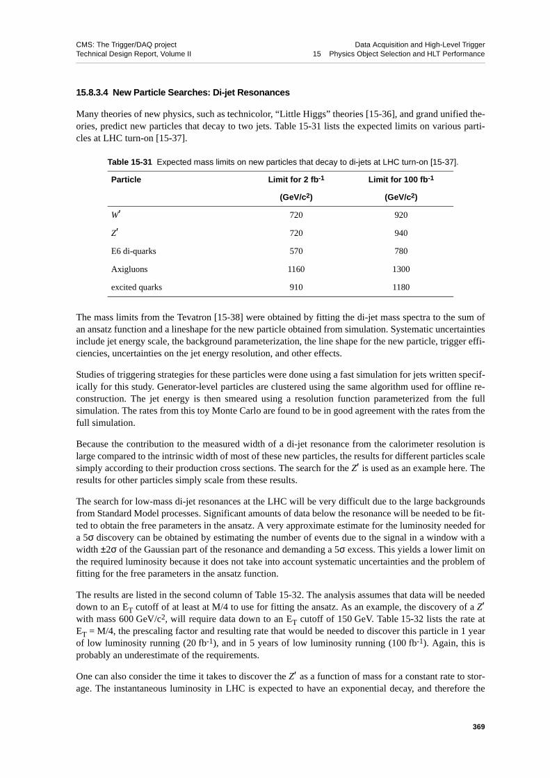
CMS: The Trigger/DAQ project Data Acquisition and High-Level TriggerTechnical Design Report, Volume II 15 Physics Object Selection and HLT Performance
15.8.3.4 New Particle Searches: Di-jet Resonances
Many theories of new physics, such as technicolor, “Little Higgs” theories [15-36], and grand unified the-ories, predict new particles that decay to two jets. Table 15-31 lists the expected limits on various parti-cles at LHC turn-on [15-37].
The mass limits from the Tevatron [15-38] were obtained by fitting the di-jet mass spectra to the sum ofan ansatz function and a lineshape for the new particle obtained from simulation. Systematic uncertaintiesinclude jet energy scale, the background parameterization, the line shape for the new particle, trigger effi-ciencies, uncertainties on the jet energy resolution, and other effects.
Studies of triggering strategies for these particles were done using a fast simulation for jets written specif-ically for this study. Generator-level particles are clustered using the same algorithm used for offline re-construction. The jet energy is then smeared using a resolution function parameterized from the fullsimulation. The rates from this toy Monte Carlo are found to be in good agreement with the rates from thefull simulation.
Because the contribution to the measured width of a di-jet resonance from the calorimeter resolution islarge compared to the intrinsic width of most of these new particles, the results for different particles scalesimply according to their production cross sections. The search for the Z′ is used as an example here. Theresults for other particles simply scale from these results.
The search for low-mass di-jet resonances at the LHC will be very difficult due to the large backgroundsfrom Standard Model processes. Significant amounts of data below the resonance will be needed to be fit-ted to obtain the free parameters in the ansatz. A very approximate estimate for the luminosity needed fora 5σ discovery can be obtained by estimating the number of events due to the signal in a window with awidth ±2σ of the Gaussian part of the resonance and demanding a 5σ excess. This yields a lower limit onthe required luminosity because it does not take into account systematic uncertainties and the problem offitting for the free parameters in the ansatz function.
The results are listed in the second column of Table 15-32. The analysis assumes that data will be neededdown to an ET cutoff of at least at M/4 to use for fitting the ansatz. As an example, the discovery of a Z′with mass 600 GeV/c2, will require data down to an ET cutoff of 150 GeV. Table 15-32 lists the rate atET = M/4, the prescaling factor and resulting rate that would be needed to discover this particle in 1 yearof low luminosity running (20 fb-1), and in 5 years of low luminosity running (100 fb-1). Again, this isprobably an underestimate of the requirements.
One can also consider the time it takes to discover the Z′ as a function of mass for a constant rate to stor-age. The instantaneous luminosity in LHC is expected to have an exponential decay, and therefore the
Table 15-31 Expected mass limits on new particles that decay to di-jets at LHC turn-on [15-37].
Particle Limit for 2 fb-1 Limit for 100 fb-1
(GeV/c2) (GeV/c2)
W′ 720 920
Z′ 720 940
E6 di-quarks 570 780
Axigluons 1160 1300
excited quarks 910 1180
369

CMS: The Trigger/DAQ project Data Acquisition and High-Level TriggerTechnical Design Report, Volume II 15 Physics Object Selection and HLT Performance
rates at a given threshold also decrease exponentially. Applying this model, and using dynamic prescalingto keep the rate to storage constant, the prescaling factor also decreases exponentially with time.
Table 15-32 also lists the time to discovery for three prescaling scenarios:
Table 15-32 Minimum requirements to discover a Z′ decaying to two jets. The first column, “Luminosity”, givesthe integrated luminosity needed to have a 5σ Z′ signal, the second column, “M/4”, gives the threshold on the jettrigger ET used to determine the luminosity, the third column, “rate”, gives the rate for the single jet trigger at thatthreshold, the fourth column, “1 year” gives the rate needed to acquire the events within 1 year (20 fb-1) (andalso, in parenthesis, the prescaling factor required and the number of events), the fourth column, “5 years”,gives the rate and prescale to acquire that number of events in 5 years. The last three columns give the timerequired to acquire, under three different prescaling scenarios described in the text, the same number of events.
Z′ massLumi-nosity M/4 rate
rate(prescale) (events)
1 year
rate(prescale)
5 years fixed rate
fixed prescale
storage rate of 100Hz
(TeV/c2) fb-1 GeV Hz Hz Hz years years years
0.6 1.4 150 800 56 (14.2) (40×106) 11(71) 1.65 2.8 1.5
0.8 2.3 200 200 23 (8.7) (26×106) 4.5 (44) 0.68 1.15 0.63
1.0 4.3 250 55 12 (4.7) (26×106) 2.3 (24) 0.35 0.59 0.33
1.2 7.3 300 25 9 (2.7) (33×106) 1.9 (13) 0.37 0.46 0.37
1.4 14 350 11 7.8 (1.4) (55×106) 1.6 (7) 0.70 0.70 0.70
1.6 20 400 6 6 (1) (60×106) 1.2 (5) 1.0 1.0 1.0
1.8 31 450 3.5 - 1.1 (3.2) 1.55 1.55 1.55
2.0 52 500 2 - 1.1 (1.9) 2.6 2.6 2.6
Figure 15-85 Time for the significance for the number of dijet resonance events in a window around the reso-nance mass to have a 5 σ significance over the background for the 3 prescale schemes described in the text.
Zprime mass (TeV)0.6 0.8 1 1.2 1.4 1.6 1.8 2 2.2 2.4
tim
e (y
ears
)
0
0.5
1
1.5
2
2.5
3
3.5
4
dynamic prescale to 20 Hz for dijets
fixed prescale, 20 Hz initial rate
dynamic prescale to 100 Hz total
370

CMS: The Trigger/DAQ project Data Acquisition and High-Level TriggerTechnical Design Report, Volume II 15 Physics Object Selection and HLT Performance
• an exponential luminosity decay with time constant of 10 hours, during a beam fill of 10 hours, anda fixed rate to storage for the single jet trigger of 20 Hz;
• a fixed prescale, with a rate to tape for the single jet trigger of 20 Hz at 2×1033 cm-2s-1;
• an exponential luminosity decay with a 10-hour lifetime, during a beam fill of 10 hours, a fixedrate to storage for all triggers of 100 Hz, taking an initial rate for the single-jet triggers of 5 Hz.
All three scenarios assume 20 fb-1 per year for low luminosity running. Figure 15-85 shows the time todiscovery for these three options.
15.8.3.5 Standard Model Physics
The measurement of W and Z boson production properties, and especially their couplings, will be one ofthe topics which will be studied at the LHC. Deviations may hint at new physics. First manifestations ofSupersymmetry may have to be discriminated against a background of W+jets and Z+jets events. Thesame holds for heavy flavour physics and, in particular, studies of the top quark, where couplings, rare de-cay modes, spin characteristics and correlations have to be studied. W, Z and top-quark production alsoprovide key tests of QCD.
The main channels for analysis of W and Z-bosons at LHC will be their leptonic decays. The efficienciesfor W and Z-bosons have been determined in Section 15.2 for electrons and in Section 15.3 for muons.The production rates for W→eν and Z→ee are approximately 20 nb and 2 nb respectively and thereforelead to a rate of events of 40 and 4 Hz respectively at low luminosity.
About 60% of the produced W-bosons will have an electron in the fiducial volume of the ECAL |η| < 2.5.Using the single electron trigger the overall efficiency is 67% (59%) at low (high) luminosity.
Similar numbers are obtained for the muon decay channel. Here the geometrical fiducial acceptance of|η| < 2.1 is about 50%, and the trigger acceptance using the single muon trigger as defined in section 14-3is 69% at low luminosity and 42% at high luminosity. For the channel Z→µµ, with muons in the fiducialvolume, the trigger acceptance is larger and amounts to 92 % (86 %) at low (high) luminosity.
The efficiency for top quarks via the decay tt→µ+X is also rather high, and amounts to 72% at low lumi-nosity. Detailed studies of top production and decay properties will undoubtedly be among the main activ-ities of the first years of running and the ground work against which searches for new phenomena (andpotential discoveries) will have to be compared and judged. Top-quark production is often the main back-ground in various searches, foremost in SUSY searches, and for this reason it will have to be understoodthoroughly early on in the LHC physics program.
15.8.4 Summary
A draft “trigger table” for the Level-1 Trigger and the High-Level Trigger selection at a “start-up” lumi-nosity of 2×1033 cm-2s-1 has been shown. The assumption of this table is a total DAQ bandwidth of50 kHz. It has been shown that high efficiencies for most physics objects are attainable with a selectionthat remains inclusive and avoids detailed topological or other requirements on the event. The overallCPU requirement of this selection is approximately 300 ms on a an Intel 1 GHz Intel Pentium-III CPU.
Much more sophisticated trigger requirements can, and most likely will, be employed. As an example, ata minimum, as the instantaneous luminosity drops throughout a fill of the LHC bandwidth will be freedfrom the triggers discussed here. This additional bandwidth can be reallocated to the same triggers by de-
371

CMS: The Trigger/DAQ project Data Acquisition and High-Level TriggerTechnical Design Report, Volume II 15 Physics Object Selection and HLT Performance
creasing the thresholds, as in the example of the di-jet resonance dynamic prescale factors discussed inthis chapter.
The additional bandwidth may also be used in introducing new triggers, e.g. for B-physics, a topic thathas not been described so far. Introduction of such triggers is then purely an issue of whether there are ad-equate CPU resources for the selection of the relevant events. The systematic optimization of the track re-construction code and the extensive use of “regional” and “conditional” track reconstruction allow for thevery fast search for and the full reconstruction of B-meson decays. Further, the optimization of the track-ing code indicates that it can be applied to the full Level-1 event rate at both low and high luminosity.This would extend and complement the current “Level-2” selections described in this chapter. There isongoing work in the area of optimization of the tracking code and of its application in various parts of theselection. Two examples which include a “Level-2” tracker-based selection and a b-tag are described indetail in Appendix G. The same Appendix includes a discussion of selected B-physics channels.
The selection presented in this chapter indicates that it is possible to provide the HLT selection of 1:1000in a single processor farm. Furthermore, the full event record is available, and the software that imple-ments all algorithms can be changed and extended quite easily. The CMS HLT system has great flexibilityand provides much room both for improving the selection of the various physics channels, as well as foradjusting to unforeseen circumstances resulting from bad beam conditions, high background levels ornew physics channels not previously studied.
372

CMS: The Trigger/DAQ project Data Acquisition and High-Level TriggerTechnical Design Report, Volume II 15 Physics Object Selection and HLT Performance
15.9 References
15-1 CMS Coll.,“The Trigger and Data Acquisition project, Volume I, The Level-1 Trigger, Technical Design Report”, CERN/LHCC 2000-038, CMS TDR 6.1, 15 December 2000.
15-2 E. Meschi et al., “Electron Reconstruction in the CMS Electromagnetic Calorimeter”, CMS Note 2001/034.
15-3 P. Aspell et al., “Results from the 1999 Beam Test of a Preshower Prototype”,CMS Note 2001/001.
15-4 See, for example, J.P. Peigneux et al., “Results from Tests on Matrices of Lead Tungstate Crystals Using High Energy Beams”, Nucl. Instrum. Methods A378 (1996) 410.
15-5 I. Puljak, Thèse de Doctorat de l’Université Paris VI, 21 Sept 2000.
15-6 CMS Coll.,“The Electromagnetic Calorimeter Project, Technical Design Report”, CERN/LHCC 97-33, CMS TDR 4, 15 December 1997.
15-7 G. Daskalakis and K. Lassila-Perini, “Jet rejection using the pixel matching for the low and the high luminosity”, CMS Note 2002/039.
15-8 V. Innocente, M. Maire, E. Nagy, CERN program library long writeup W5013-E, GEANE.
15-9 G. Bruno et al., “Local reconstruction in the muon detectors”, CMS Note 2002/043.
15-10 N. Amapane, M. Fierro, M. Konecki, “High-Level Trigger Algorithms for Muon Isolation,” CMS Note 2002/040.
15-11 Jet Algorithm Working Group, “Towards standard Jet Algorithms for Run II”, http://niuhep.physics.niu.edu/~blazey/jet_alg/jet_alg.html
15-12 D. Green et al., “Energy Flow Objects and Usage of Tracks for Energy Measurement in CMS”, CMS Note 2002/036.
15-13 R. Kinnunen and A. Nikitenko, “Study of H(SUSY) -> Tautau -> l + Tau Jet + Etmis in CMS”, CMS Note 1997/106.
15-14 D. Denegri and R. Kinnunen, ”Study of H(SUSY) -> tau,tau -> h+ + h- + X in CMS “, CMS Note 1999/037.
15-15 R. Kinnunen, “Study for Heavy Charged Higgs in pp -> tH+ with H+ -> Tau + Neutrino in CMS”, CMS Note 2000/045.
15-16 J. E. Huth et al., Proceeding of Research Directions for the decade, Snowmass 1990.
15-17 S. Eno et al., “A Study of a First and Second Level Tau Trigger”, CMS Note 2000/055.
15-18 D. Kotlinski, A. Nikitenko and R. Kinnunen, “Study of a Level-3 Tau Trigger with the Pixel Detector”, CMS Note 2001/017.
15-19 G. Bagliesi, S. Gennai and G. Sguazzoni, “A L2 Trigger for Tau Hadronic Decays with Tracker Isolation in the Low Luminosity Scenario”, CMS Note 2002/018.
15-20 G. Segneri and F. Palla, “Lifetime-based b-tagging with CMS”, CMS Note 2002/046.
15-21 The ALEPH Coll., Physics letters B 401 (1997) 163-17; also the DELPHI Coll., E. Phys. J. C10 (1999) 415.
15-22 The LEP Heavy Flavour Group,”Input Parameters for the LEP/SLD Electroweak Heavy Flavour Results for Summer 1998 Conferences”, LEPHF/98-01,http://www.cern.ch/LEPEWWG/heavy/lephf9801.ps.gz.
15-23 D. Kotlinski and A. Starodumov, “High Level Tracker Triggers for CMS”, Presented at: Vertex 2001, Brunnen Switzerland, September 200,CMS Conference Report 2002/003.
373

CMS: The Trigger/DAQ project Data Acquisition and High-Level TriggerTechnical Design Report, Volume II 15 Physics Object Selection and HLT Performance
15-24 D. Kotlinski, “CMS Pixel Detector”, to appear in Proceedings Beauty 2002 Conference, Santago de Compostela, Spain, 17th-21st June 2002.
15-25 S. Abdoulline and D. Denegri, “On the Possibility to Observe h -> b-bbar with S/B ~ 1 in SUSY (mSUGRA), and Implications for Tracker and HCAL”, CMS Note 1997/070.
15-26 M. Winkler et al, “Estimation of Alignment Parameters, Using the Kalman Filter with Annealing”, CMS Note 2002/008.
15-27 A. Ostaptchouk et al, “The Alignment system of the CMS Tracker”, CMS Note 2001/053.
15-28 D. Futyan and C. Seez, “Intercalibration of ECAL Crystals in Phi Using Symmetry of Energy Deposition”, CMS Note 2002/031.
15-29 CMS Coll.,“The Hadronic Calorimeter Project, Technical Design Report”, CERN/LHCC 97-31, CMS TDR 2, 20 June 1997.
15-30 CMS Coll.,“The Muon Project, Technical Design Report”, CERN/LHCC 97-32, CMS TDR 3, 15 December 1997.
15-31 F. Matorras et al., “Offline muon station alignment using the inclusive mu LHC production”, CMS Technical Note 1996/005.
15-32 H. Baer et al., Phys. Rev. D 58 (1998) 075008.
15-33 O.J.P. Eboli and D. Zeppenfeld, Phys. Lett. B495 (2000) 147.
15-34 B. DiGirolamo et al., “Experimental Observation of an Invisible Higgs Boson at the LHC”, Workshop on Physics at TeV Colliders, Les Houches, 2001, the Higgs Working Group: summary report, hep-ph/0203056.
15-35 LEP Higgs Working Group, hep-ex/0107032
15-36 M. Schmaltz, “Introducing the Little Higgs”, hep-ph/0210415.
15-37 D. Amidei and R. Brock, “Future Electroweak Physics at the Fermilab Tevatron: Report of the TeV_2000 Study Group”, FERMILAB-PUB-96/08.
15-38 F. Abe et al. (CDF Collaboration), Phys. Rev. Lett. 74 (1995) 3538.
374

CMS: The Trigger/DAQ project Data Acquisition and High-Level TriggerTechnical Design Report, Volume II 16 Computing Services
16 Computing Services
Following execution of High-Level Trigger (HLT) algorithms and other processing in the Filter Systems,data are transmitted to the online and offline Computing Services. These data include events selected bythe HLT for physics analysis, events selected for calibration, some fraction of events rejected by the trig-gers, collected calibration information, and a wide variety of data for online monitoring. Some data willbe processed online and some will be transmitted to offline systems for event reconstruction, selection,and other offline processing.
This chapter describes the online Computing Services as well as the interface between online and offlinecomputing. Many of the tasks executing in the online Computing Services, such as monitoring and cali-bration, have been described elsewhere in this Technical Design Report (TDR) or in sub-detector TDRs.This chapter focuses on the general applications running on the online Computing Services and the organ-ization of those Computing Services. The full description of the Tier-0 offline Computing Services will begiven in the forthcoming Computing TDR. In this chapter we focus on the interface between online andoffline and on the requirements for prompt initial offline processing of the data.
16.1 Introduction
The online Computing Services must be highly reliable yet low cost. In particular, the costs of manage-ment, maintenance and operations must be kept to a minimum. This clearly implies that the online Com-puting Services should be one system managed for use by all the calibration, monitoring, and otherprocesses. In particular, all subdetector processes should run on a uniform Computing Services system.The system must be upgraded frequently as computing hardware and software improves. Again, this callsfor a uniform system comprising all online Computing Services.
According to the design of the event builder, all events and calibration data collections are first sent to oneof the Filter Units. There, the HLT is used to select events for storage and analysis. In addition, the FilterUnits may be used to accumulate and pass on calibration or monitoring information to processes runningon the Computing Services. It is expected that there will be a very significant stream of calibration datarequiring significant computing resources. It is expected that monitoring to ensure data quality will becomprehensive and therefore a large number of monitoring processes will also require computing re-sources. Several other online processes, some of which are described in this chapter, will also execute onthe online Computing Services.
The interface between online Computing Services and the offline processing systems is designed to pro-vide for maximum data collection efficiency and maximum data quality. This chapter states some of therequirements on that interface, necessary to achieve that efficiency and quality.
Full reconstruction of events selected by the HLT will take place in the offline “Tier-0” computer falici-ties. Some of the calibration and monitoring tasks will depend on this initial reconstruction step. There-fore, the timely offline reconstruction of selected events is a requirement of the online system.
Some general aspects of planned computing systems, as they are understood today, are also described be-low. Certainly there will be major improvements in computing hardware, software, and operating systemsby the time the LHC starts running. There will also likely be qualitative changes in the optimal way to de-sign a computing system. Nevertheless, a general description of Computing Services as would be de-signed today is worthwhile.
375

CMS: The Trigger/DAQ project Data Acquisition and High-Level TriggerTechnical Design Report, Volume II 16 Computing Services
16.2 Architecture
The Filter Farm, Computing Services, and the connection to the offline Tier-0 centre are displayed inFigure 16-1. Accepted events and other data from the Filter Units (FU) are passed through the ComputingServices Network to the appropriate compute Server Unit (SU). Processes on the SU then complete theonline processing of the data.
Processes on the FU collect accepted events, divide them into streams, and forward them for offlineprocessing. In normal operation, the accepted events are immediately sent on to the offline Tier-0 centrefor the initial offline processing step. The data are saved in the Raw Data Store until the result of the pro-duction has been fully validated. Normally events will be promptly forwarded to a Processing Unit (PU).The result of the reconstruction will be saved along with the raw data in a large Object Database.
Most monitoring and calibration processes are completed online in the SU. For example, a monitoringprocess executing on one of the SU subscribes to a particular type of data, collects it, processes it, thenstores the result for display, validation and use in other analyses. An online calibration task works in asimilar way.
A possible network configuration, shown below, features a dedicated network for the initial eventprocessing. The benefit of this is independence from other offline processes.
16.2.1 Computing Services Network
Data from the Filter Systems are transmitted to Computing Services on a high-speed network the “Com-puting Services Network”. It is possible to transmit data from any part of the Filter System to any part ofthe Computing Services. The Computing Services Network is also used to transmit data for offline stor-age and processing.
The output event rate from one FU node is very small, well under one Hz. Even the aggregate Filter Farmoutput event rate is quite small. The data rate due to calibration and monitoring will likely be higher thanthe data rate due to accepted events; however, it will still be a small fraction of the input data rate to the
Figure 16-1 Architecture of the Computing Services.
ExpressLine PU PU PU
HeadNode
SU SU
FUFUFilter Unit
FU FU
Filter Data Network
Tier-0 On-line Network
Online Data Buffer
StorageSystem
RawData Store
ObjectDatabase
Tier-0 Off-line Network
376
CMS: The Trigger/DAQ project Data Acquisition and High-Level TriggerTechnical Design Report, Volume II 16 Computing Services
Filter System. Therefore, the Computer Services Network will be inexpensive compared to the Filter DataNetwork. It will likely be built from multiple Ethernet switches connected by trunks. It is even possiblethat hardware components of the Filter Data Network can be used in the implementation of the ComputerServices Network.
16.2.2 Computing Services Processor Cluster
Each unit of the Computing Services cluster of processors is labelled a SU in the figure. The cluster con-tains of order 100 dual-processor nodes. The processes running on the SU are CPU limited in general, asare those on the FU and PU. Some of the nodes have a very high input data rate, like the FU. Therefore,the requirements for the SU nodes are very much like those for the FU.
The SU should be interchangeable from the point of view of the online computing task such as monitor-ing and calibration. The system can be made more reliable by having a pool of unused nodes that can beused to replace any node that fails. The compute nodes will not be used for permanent storage of data sothat processes can be easily migrated to other nodes.
The Computing Services cluster is managed by one or two head nodes depending on whether sub-clustersare called for. The head nodes manage the tasks on the cluster. Some tasks are resident on particular nodesof the cluster while others run in batch queues on the head node and are subsequently assigned to availa-ble SUs. The configuration of resident tasks can be easily modified since the tasks themselves do not de-pend on which node they run.
The online Computing Services will use a single operating system that is supported by both online and of-fline software and is highly functional, inexpensive, and supports the most cost-effective computing hard-ware. The baseline operating system of today is Linux.
16.2.3 Computing Service Storage Systems
All data related to the calibration and monitoring processes running on the online Computing Serviceswill be stored on reliable storage systems like RAID arrays. This will require a high-bandwidth, low-la-tency connection between processors and storage systems. The storage systems should be backed-up fre-quently without loss of data taking efficiency.
16.2.4 Online Data Buffer
If the connection to the offline Tier-0 centre is temporarily lost, data collection should proceed uninter-rupted. A reasonable data buffer of 100 TB is sufficient to survive a one-week interruption of data trans-mission from the experiment. It also will allow useful local operation under many conditions. This shouldbe a reliable (RAID) disk buffer. In the event of a problem with the Data Buffer, data can be sent unbuff-ered to the offline Computing Services.
16.2.5 Estimate of Computing System Size
It is difficult to make an accurate, bottom-up estimate of the required size of the online Computing Serv-ices. A sensible estimate based on resource allocation is ~10% of the size of the farm or at least 100 proc-
377

CMS: The Trigger/DAQ project Data Acquisition and High-Level TriggerTechnical Design Report, Volume II 16 Computing Services
essors at start-up. Calibration or monitoring tasks that require more resources should be carefullyreconsidered.
The storage needs will be dominated by the online Database. Monitoring, calibration, and other tasks willlikely make use of some additional storage; on the order of 200 Terabytes at start-up, in addition to the on-line data buffer.
16.2.6 Network Connection to Offline Computing Services
While the Filter Farm and online Computing Services will be at the experimental site, it is expected thatthe offline Tier-0 centre will be located on the Meyrin CERN site. An adequate network connection be-tween the Filter Farm and remote Computing Services is required. A 5 Gb/s network link devoted to mov-ing data will be sufficient even under adverse conditions when a backlog of data must be transmitted.Reliable transmission using TCP/IP over Ethernet would be the most straightforward choice today.
16.2.7 Tier-0 Networks
Subject to technology changes, the Tier-0 networks are expected to be based on Gigabit Ethernet with thepossible use of 10-Gigabit Ethernet in some areas. The capability exists to have an “online” network ded-icated to the initial processing step. This minimizes possible interference from other computing tasks. Thededicated network could be physical or virtual.
16.2.8 Tier-0 Raw Data Store
It is important to minimize the loss of raw data due to processing failures; therefore, the data coming fromthe detector will be stored until the result production is fully validated. A large data store could be usedfor this purpose and as a data buffer in the event that the processor system cannot keep up with the datarate from the detector. A disk buffer of 50 TB is appropriate. If more buffer space is needed, the timeneeded to process 50 TB of data is such that mass storage may be used in the event this buffer becomesfull.
16.2.9 Tier-0 Processing Farm
The offline Tier-0 processing farm is currently estimated to contain 500 commodity dual-processor PCs,each of which will have approximately eight times the performance of the high end systems available inlate 2002. These nodes are called Processor Units (PU). The processors will be used for the initialprocessing step, for reprocessing of data, for physics analysis, and for various other tasks. For manage-ment purposes, the farm may be arranged in sub-farms to ensure appropriate scaling.
For ease of management and operation, the PU will not be used for storage. The local disk contains theoperating system and any temporary files needed for processing. In this way, PUs can be easily added orremoved. The operating system can be upgraded at will.
The performance of the PU on the CMS reconstruction task is the most important parameter of the sys-tem. Experience has shown that the reconstruction task makes efficient use of the CPU; approximately85% utilization is a reasonable estimate. A 10% loss of efficiency for hardware or software maintenancecan be expected.
378

CMS: The Trigger/DAQ project Data Acquisition and High-Level TriggerTechnical Design Report, Volume II 16 Computing Services
16.2.10 Object Database
The Object Database is a major component of the CERN Tier-0 centre. It will store raw data, reconstruct-ed objects and calibration constants, as well as production and analysis status. Ultimately, it will containmany petabytes of data.
The experience of modern High Energy Physics collaborations is that the Database is one of the mostcomplex systems in the experiment. Optimised use of a database can result in significant resource savingsalbeit it at a price to be paid. The onsite database will likely require a good deal of care and maintenance.Corruption of the data must be avoided. Some downtime will probably be introduced to do the mainte-nance, leading to inefficiency in the system. It is also important that physics discoveries not be delayeddue to problems with the database so discovery channels will be directed to an Express Line analysisstream in addition to a standard stream using the large database. The details of the Database are beyondthe scope of this document.
16.3 Computing Services Tasks
This section details how the primary Computing Services tasks will execute on the online ComputingServices farm.
16.3.1 Computing for Online Monitors
Every aspect of the detector performance, rates, accelerator performance, readout electronics, Level-1Trigger, Event Builder, Filter System, HLT software, communications networking, computer systems,calibration, Run Control, offline reconstruction, offline selection, and physics performance will be moni-tored online. The sources of monitoring data are spread over the online and offline systems. Monitoringdata typically pass through some manager node. It is then transmitted to client nodes in Computing Serv-ices. Monitoring processes subscribe to particular data categories and subsequently receive those data.
For the smooth operation of the experiment, both the monitoring software and the computing hardware onwhich it executes will be standardized to provide ease of long-term maintenance and operation of themonitors.
16.3.2 Computing for Online Calibrations
Detector systems rely on calibrations that will be performed both online and offline. Because the LHCevent rate is so large, highly accurate calibrations can be made in a realatively short time. The Tracker andMuon systems rely on good alignment. While the systems are designed to be as stable as possible, the ex-perience of many experiments is that alignments are not always stable. The electromagnetic calorimeterhas very good energy resolution but suffers from changes in light output with temperature and radiation.These are examples of detectors that may require that up-to-date calibrations be available for initialprocessing. Online calibrations will be completed on a time scale such that they may be used in the initialprocessing step.
Most of the calibration will take place in the online Computing Services. This includes the use of datataken purely for calibration purposes and the calibration of electronics. It is also planned that some as-pects of detector alignment will take place online. Again, these tasks will be executed on processors in theComputing Services farm.
379

CMS: The Trigger/DAQ project Data Acquisition and High-Level TriggerTechnical Design Report, Volume II 16 Computing Services
Calibration data may be in the form of special calibration blocks, full or partial events selected for calibra-tion, or full events selected for physics analysis. In general, all these data are assembled and sent to a Fil-ter Unit for processing. The FU transmits calibration data to the appropriate calibration process on theComputing Services system for further analysis, accumulation of data, and computation of a calibrationresult. The result is sent to the database for use both offline and online.
16.3.3 Other Online Processes
Many other online applications run on the Computing Services. Examples include event displays, histo-gram displays, electronic logbooks, validation tasks, expert systems, and calculations of optimal triggerthresholds and prescale factors.
16.4 Other Online Services
16.4.1 Control Room Workstations
Workstations with large displays are provided in the control room to interact with the various tasks run-ning on Computing Services. For example: monitoring and calibration processes must be controlled andchecked; event displays must be controlled, calibrations must be validated; entries must be made in elec-tronic logbooks. These workstations can also be used for other tasks.
About ten workstations should be sufficient for interaction with Computing Services tasks. These do notinclude the RCMS and DCS systems.
16.4.2 Control Room Displays
Large, high-resolution displays in the control room are used to make monitoring and event displays visi-ble over a wide area of the room. Technology advances are expected to make very large displays cost ef-fective. Special workstations will be needed to drive these displays. At this time, plasma displays orprojected displays would be the technologies of choice.
16.4.3 Event Display Streams
Online event displays are useful for many purposes. To make use of them, streams of event types for dis-play are selected in the Filter System. These include various types of physics streams, calibration streams,error streams, and clearly, events selected for express line processing.
16.4.4 Local Resources for General Computing
In addition to workstations located in the control room, a pool of about 20 additional workstations shouldbe provided for online use. These may support alternative operating systems and software as well as thestandard OS and CMS software. Wireless connections and convenient power for laptops should also besupported all around point 5. This will help provide access to computing during peak activity periods.
380

CMS: The Trigger/DAQ project Data Acquisition and High-Level TriggerTechnical Design Report, Volume II 16 Computing Services
16.4.5 Support for Remote Control Rooms
The online Computing Services will provide for remote access to the control room so that detector expertsand shift-takers can work remotely. This means that all the displays can be shared efficiently over compu-ter networks; that monitoring and calibration can be controlled remotely; and that audio and video con-nections are available.
Remote controlled video cameras with pan and zoom facility will help enable physicists outside of point 5to inspect the condition of many systems including readout electronics, gas systems, control systems, aswell as all information available in the control room. Video conferencing facilities in the control roomwill enable communication between local and remote shift personnel.
16.4.6 Filter Farm Use During Shutdown
The FU nodes and the PU nodes of the Computing Services could be essentially the same. They are bothoptimised to perform well running reconstruction software. During long shutdowns of the data taking, theFilter Farm should be used to augment the capacity of the Tier-0 centre to the extent that this does not in-terfere with maintenance and development of the online systems. The primary use is likely to be reproc-essing of data. The additional requirements that this use will place on the online Computing Services arenot severe given good networking between point 5 and the Tier-0 centre.
16.5 Interface to Offline Computing
The interaction of offline processing, calibration, and monitoring with the online system places require-ments on both the online and offline systems. The primary requirement on the offline system is forprompt, reliable processing.
The initial reconstruction, selection, and calibration processing for the data require that very significantoffline computing resources be highly available during data taking. The HLT, which has access to the fullevent information, has been shown to select a very pure data sample. Nearly all the events passing theHLT requirements will be used in a physics analysis, background measurement, or calibration process.
For many reasons, all the data must be processed promptly. Calibrations of detector components will beperformed then used in the reconstruction process. These calibrations may also be used for online moni-toring, HLT algorithms, and detector performance assurance. Prompt processing also minimizes diskbuffer sizes and access to mass storage.
The initial processing task is similar to that in other High Energy experiments. A large number of inde-pendent events must be reconstructed or used for calibration. These events can be easily processed in par-allel so large farms of inexpensive computers can be used.
Since computing resources will be scarce, processors should not be left idle. During periods of data-tak-ing, a large fraction of the on-site processor resources will be devoted to the initial processing of datafrom the detector and, during periods when the experiment is not collecting data, resources will be shiftedto other tasks. The ability to allocate computing resources, including Filter Farm nodes, to tasks like re-processing will help satisfy the large on-site computing needs of CMS. Reliability of the processing sys-tem is also of great importance. The less organized computing activities, like physics analysis, must notmake the system used for initial processing unstable. It should be possible to segregate the nodes allocat-
381

CMS: The Trigger/DAQ project Data Acquisition and High-Level TriggerTechnical Design Report, Volume II 16 Computing Services
ed to initial processing from the rest of computing services, yet allow allocation to various tasks depend-ing on running conditions.
16.5.1 Requirements
The requirements for the initial processing step can be easily understood, however, some important num-bers are estimates that are uncertain to a factor of two. For example the processing power needed to re-construct an event can only be estimated from Monte Carlo. It will clearly depend on running conditionsand detector performance. Projections of the price performance of future computing systems are alsoclearly uncertain by at least a factor of two.
The expected rate of events satisfying the HLT is about 100 Hz, at least at a luminosity of 2×1033 cm-2s-1.There will certainly be periods during which the trigger rate is above this average value due to runningconditions. A value as high as 200 Hz can perhaps be expected. At full luminosity, the average event sizeis conservatively estimated to be 1 MB while at low luminosity the event size will be reduced to about300 kB due to the reduction in pile-up.
The current estimated processor time needed to reconstruct an event is 3000 SI95-seconds. With 109
events per year, the average processing power needed for the initial processing step is 100 kSI95. If theHLT rate is 200 Hz, the instantaneous need for processing power is 600 kSI95 to keep pace with incomingdata. Ideally 600 kSI95 should be available, however, 300 kSI95 would be sufficient if processing ofsome data streams is delayed until a break in data collection. This translates into about 1000 high per-formance dual processors in 2007.
Since the instantaneous need for processors is larger than the average rate, it must be possible to allocateidle processors to reprocessing or physics analysis routinely when data taking stops. It should also be pos-sible to allocate Filter Farm nodes to reprocessing during long breaks in data taking.
16.5.2 Offline Monitors
There are three types of information to be monitored offline. First, information about the status of the dataprocessing must be regularly updated. Examples include the latency of events in each stage of the system,the processing time as a function of trigger type, the number of recoverable exceptions, the utilization andstatus of the processing nodes, and the network utilization will be monitored. Second, the calibration re-sults, detector performance, rates into physics channels, luminosity, beam conditions, beam location andbeam size will be monitored. It would be beneficial if these could be fed back to the online system withinan hour. Third, a comparison of the offline selection algorithms with the HLT results will be monitored.
16.5.3 Initial Processing of the Data
Processing involves reconstruction of events, the addition of persistent reconstruction information to theraw data, the use of physics events to extract calibration and detector performance information, the tag-ging of physics events with overall event parameters, the selection of physics events as candidates for dif-ferent physics processes and analyses, the separation of events into streams to optimise the data access forfurther analysis, and the updating the Object Database.
Ideally, the initial processing of the data coming from the detector should take place on a time scale ofabout 30 minutes, although this number is quite uncertain. To cover the possibility that calibration or de-
382

CMS: The Trigger/DAQ project Data Acquisition and High-Level TriggerTechnical Design Report, Volume II 16 Computing Services
tector performance information may be fed back to the online system, the offline Computing Services willbe designed to work on this time scale.
16.5.4 Rolling Calibration
Although, as previously stated, most of the calibration will take place in the online Computing Services,some calibration and alignment will naturally come out of the full reconstruction of physics events. Cali-bration will certainly be an important part of the initial event processing. The calibration streams mayeven be processed first so that the results can be used in the reconstruction of physics events.
A “Rolling Calibration”, in which the calibration results derived from one short time period are used inthe next short time period to reconstruct, cannot be ruled out a priori. Modern HEP collaborations like Ba-Bar have made this work successfully. The Computing Services will allow for a Rolling Calibration, im-plying prompt initial processing of data.
16.5.5 Express Line
Some types of events, for example “golden” Higgs candidates, spectacular multi-lepton events, or eventswith huge missing transverse energy are so interesting that they should be analysed immediately with theresult fed back to the online crew and the physics crew on shift. There are many possibilities for backlogsand analysis delays in the standard processing stream so a separate “Express Line” makes sense. An eventpicked in the HLT for Express Line analysis would be sent immediately to a processor with no backlog. Aseparate output stream to disk will assure that the results of the Express Line are available. Express Lineevents should be so rare that duplication of the analysis in the standard stream will not be a significantoverhead.
The Express Line will give feedback to the online crew in a matter of minutes. To minimize softwareoverhead, the Express Line can use the same software as used in the standard production stream. ExpressLine processing could be located in the Filter Farm or in the central Computing Services, depending onperformance of the system. Migration from one location to the other should be transparent.
16.5.6 Offline Software
Effective development projects are under way for all aspects of the CMS software. By using prototypesoftware for this TDR a large base of users has been achieved. The same software will be used online andoffline to minimize delays in migrating physics selection to the HLT. A discussion of the CMS software isclearly beyond the scope of this document, however, the software does impact our design and the scope ofthe Computing Services. The time required to reconstruct events, the memory requirements, and the needfor network I/O are all based on projections from the current performance of the software prototypes. Sig-nificant Monte Carlo production, event reconstruction and analysis have been done, with the prototypesoftware, on large clusters of Linux dual processor nodes, for this TDR.
16.5.7 Quality Assurance, Validation, and Processing Control
The online shift crew will be responsible for Quality Assurance of the data and detector. This may in-clude prompt feedback from the offline processing. Another major QA task is the assurance that the re-
383

CMS: The Trigger/DAQ project Data Acquisition and High-Level TriggerTechnical Design Report, Volume II 16 Computing Services
construction and calibration processing is functioning well. Intervention from a processing shift crew orfrom experts is likely to be needed on many occasions.
There will be professional operators of the CERN computing services as well as detector experts and ashift crew from the experiment to run the data processing. As with other shift crews, remote participationwill be very valuable. It increases the pool of experts and allows more participation. It even offers relieffrom night shifts. A controlled method of remote access for experts and shift crew should be available.For the less expert shift crew, web based tools that are easy to learn and use will be beneficial.
Quality Assurance will continue to be automated over time but will often require the shift crew to look atdata summaries and graphs.
A key aspect of the processing chain will be its validation. Again, automatic tools are already in use buthuman intervention will likely be needed from time to time.
16.5.8 Online and Offline Computing Services Transparency
Most of the tasks described above should be executable both online and offline. This will be useful in thecase of emergencies and will allow for rapid testing. In particular, Express Line processing should be pos-sible either offline or online. Vital offline calibrations may need to migrate online in the event of networkor offline problems. In general, it should be possible to move calibration and monitoring tasks to optimisesystem performance and reliability.
16.6 Cluster Computing Systems
A very similar cluster architecture could be used to implement the Filter System, the online ComputerServices, and offline Tier-0 system used for initial processing. Recent developments have made clustersof PCs running Linux relatively easy to install and manage. Some properties of this type of computingcluster are discussed in this section.
Computing Systems will evolve over the lifetime of the experiment. This certainly implies hardware thatchanges rapidly and sometimes significantly with time. New hardware must be integrated quickly. Thisoften implies rapid evolution of the Operating System version to support new hardware.
Computing hardware research and development relevant to the CMS processing problem has been carriedout at many HEP labs and universities. In particular, CERN, the LHC computing grid project, other gridprojects, and the worldwide CMS computing effort have been very active. One of the most advanced testsof large clusters was the CMS production and reconstruction of a large sample of events aimed primarilyat this TDR. The largest and most successful production was carried out in the spring of 2002.
Outside HEP, there is also a very significant move toward large clusters of PCs. Many of these are aimedat applications that require a much tighter coupling between the processors than does the HEP applica-tion. Nevertheless, the R&D done outside HEP is also useful for CMS.
There seems to be a consensus that (rack mounted) PCs running Linux and connected over Ethernet are avery effective solution to the HEP problem. Both Pentium CPUs from Intel or similar processors fromAMD can be used. There is a competitive market in CPUs, motherboards, memory, disk drives, interfac-es, power supplies, and cases. Industry standards allow a good deal of choice among individual compo-nents.
384

CMS: The Trigger/DAQ project Data Acquisition and High-Level TriggerTechnical Design Report, Volume II 16 Computing Services
There has been steady progress from industry in delivering rapidly improving computer hardware at evermore affordable prices. It is very likely that this progress will continue for some time. Projecting the rateof progress for HEP applications into the future can be very complex. Even measuring past progress isdifficult for many reasons. For example, the applications we are interested in were never tested on pastcomputers and actually won’t run on them; computers of the more distant past were relatively expensiveand the measurement depends on just how expensive a computer is used; and finally details of the hard-ware are constantly changing and applications need to change to take advantage of new features (likehyperthreading on the P4).
It can be argued that the price performance has doubled every 18 months over the past several years. Itcan also be argued that the performance has doubled every 2 years and that the price will not continue todrop. It is pointless to get into the details of this argument here since our requirements are also uncertain.Taking the somewhat conservative position that performance will double every 2 years (at constant price),we project a factor of 4 to 8 improvement for the average PC ready at the time of LHC start-up. It can alsobe projected that memory speeds will be sufficient for HEP processes to take advantage of increased CPUperformance.
The 2001 International Technical Roadmap for Semiconductors published by the Semiconductor IndustryAssociation[16-1] lays out predictions for technology directions for the next decade, including transistordensity, chip size and clock speed. Their predictions indicate that steady progress can be made for sometime. The silicon feature size will continue to decrease allowing more gates to be put on a single chip,clock speeds to increase, and keeping power reasonable. Intel has announced a 90 nm feature size for nextyear, ahead of predictions.
There is evidence from the P4 performance that an increased number of gates does not benefit HEP appli-cations as much as some others. Hardware improvements are likely to cause changes in the optimal sys-tem. There may ultimately be a move to more CPUs on a single chip. The one clear lesson from the past isthat change is a certainty.
One cautionary note is in order. Market forces are hard to predict. It can be argued that there is no greatneed for commodity computers to continue to improve in CPU performance and that manufacturers arenot reaping great profits by making hardware improvements. It is probably true that the greatest uncer-tainty in future computer performance is due to market uncertainties, not technical hurdles.
16.6.1 Cluster Management
The management of large numbers of functionally similar nodes has progressed significantly over the lastseveral years. For example the NPACI-developed system, Rocks[16-2], allows for the management oflarge numbers of nodes with interaction with individual nodes only at the time of installation. The operat-ing system on a large cluster can be changed in a few minutes allowing rapid reconfiguration of the clus-ter for various tasks. In the Rocks system, the system partition of the local disk is considered completelyexpendable and is wiped each time the system is restarted.
Within this type of cluster management system, there are “head nodes” or manager nodes for each majortask. Processor nodes can be reassigned to tasks very quickly. For the Computing Services application, itmay be useful to dedicate networks to some of the task, like the initial processing task.
In the end, developments for the Grid will play an important role in our choice of cluster managementsoftware and batch systems, since the onsite CERN Computing Services for CMS should be integratedinto the Grid. Nevertheless, the initial processing step should probably be isolated from other Grid activi-ties.
385

CMS: The Trigger/DAQ project Data Acquisition and High-Level TriggerTechnical Design Report, Volume II 16 Computing Services
Technologies for implementing system management tasks are presently under investigation. Several com-mercial and public domain products exist, with the more recent ones being based on the DMTF standards[16-3] where the CIM (Common Interface Model) [16-4] model is used to describe the components of thesystem. This technology has been integrated with Web technologies such as XML and HTTP in the formof Web Based Enterprise Management (WBEM) [16-5].
The tools that the LCG project [16-6] will propose to manage the PC farms distributed over the futureLHC Grid network will be followed closely, since it is very likely that these tools will be the reference forall LHC experiments and could be easily adopted to also manage the online systems.
16.6.2 Current Computing Hardware
It is useful to take a snapshot of current computer hardware in September of 2002 as a point from whichto project. Systems currently being purchased are 1U rack-mounted dual 2.5 GHz Pentium 4. They give aperformance on CMS applications equivalent to 120 SI95 for the two CPUs running a total of four proc-esses to take advantage of hyperthreading. Memory speed has been measured to be 1.5 GB/s for a copy.The systems have two onboard Gigabit Ethernet interfaces. A test of one interface showed a 930 Mb/stransfer rate in TCP/IP. The key number is the CPU performance. The others are more than adequate forthe CMS farm needs. The cost of such a system is about $1900.
16.6.3 Future Computing Hardware
Assuming minimal changes in available computer architecture of the next 4 years, we can imagine thedual processor system of 2006. The dual processors will have about 2 GB of memory. Given the expectedgrowth of memory capacity, this should be very standard. The computational nodes purchased in late2002 have high-performance dual Gigabit Ethernet interfaces on the motherboard. This networkingwould be sufficient for the Farm of 2006, but low latency 10 Gigabit Ethernet will probably be standard.The nodes should have small reliable disks. Neither disk speed nor disk size is of much importance and itis possible that no disk at all will be needed.
The processor systems should have near optimal overall price performance. That is, the cost of hardwareper SI95 should be optimised without seriously impacting management and operation costs. Since a clus-ter node can be added or removed from the system without serious impact, the procurement and mainte-nance of these commodity computers will be optimised for price performance. If the Moore’s Lawimprovement continues, a processor node loses much of its value each year. After about four years, therack space becomes more valuable than the node and the node should be replaced. Since replacement witha higher performance system is a very viable maintenance option, the cost of warranties and maintenanceof the processor nodes can be minimized.
Linux is the choice for the operating system. Linux is inexpensive, supports the hardware with the bestprice performance, and is the primary development and production system for CMS software. It is likelythat the choice of operating system will change over the lifetime of the experiment.
16.7 References
16-1 Semiconductor Industry Association, http://www.semichip.org/
16-2 NPACI Rocks, http://www.rocksclusters.org/rocks-documentation/2.3/
386

CMS: The Trigger/DAQ project Data Acquisition and High-Level TriggerTechnical Design Report, Volume II 16 Computing Services
16-3 Distributed Management Task Force (DMTF), http://www.dmtf.org/
16-4 Common Interface Model (CIM), http://www.dmtf.org/standards/cim_schema_v27.php
16-5 Web Based Enterprise Management, http://www.dmtf.org/standards/standard_wbem.php
16-6 The LHC Computing Grid (LCG) Project, http://lcg.web.cern.ch/LCG/
387

CMS: The Trigger/DAQ project Data Acquisition and High-Level TriggerTechnical Design Report, Volume II 16 Computing Services
388

CMS: The Trigger/DAQ project Data Acquisition and High-Level TriggerTechnical Design Report, Volume II
Part 5Project Organization,
Costs andResponsibilities
389

CMS: The Trigger/DAQ project Data Acquisition and High-Level TriggerTechnical Design Report, Volume II
390
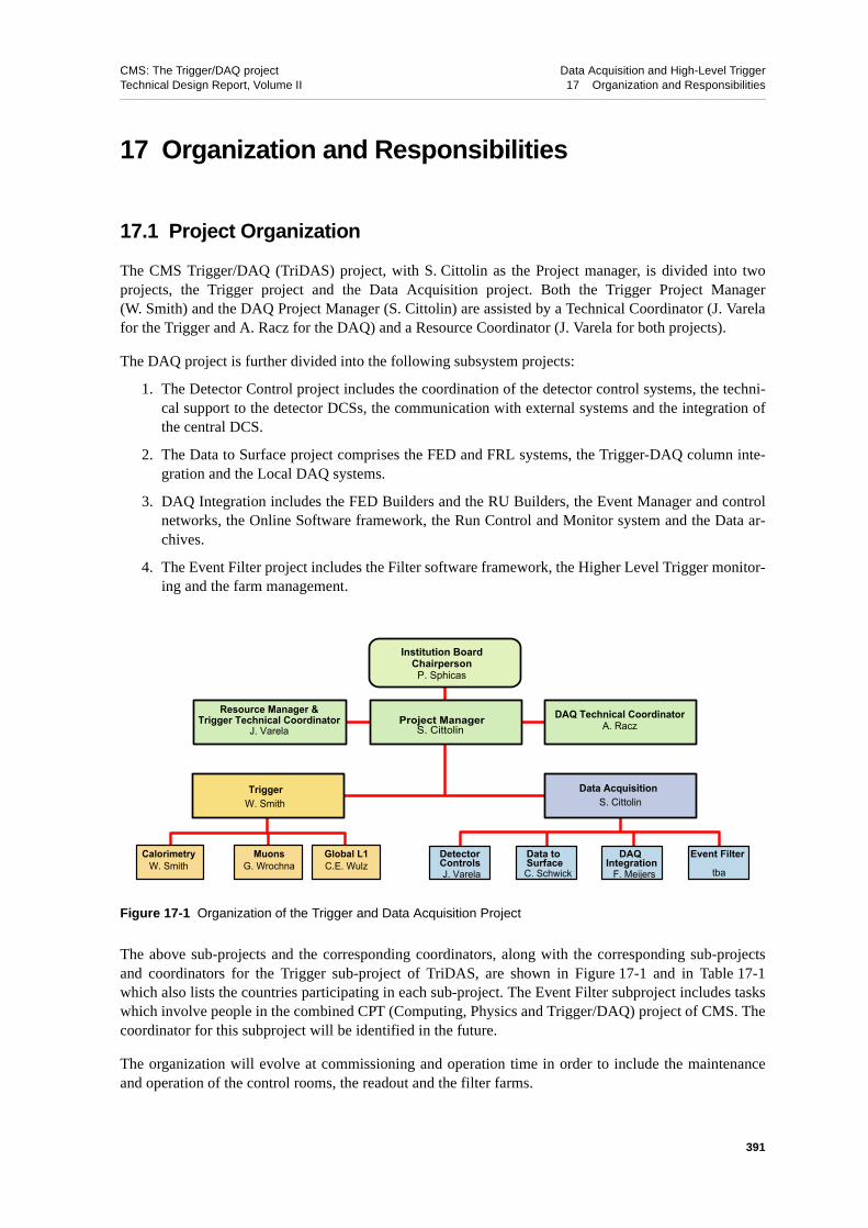
CMS: The Trigger/DAQ project Data Acquisition and High-Level TriggerTechnical Design Report, Volume II 17 Organization and Responsibilities
17 Organization and Responsibilities
17.1 Project Organization
The CMS Trigger/DAQ (TriDAS) project, with S. Cittolin as the Project manager, is divided into twoprojects, the Trigger project and the Data Acquisition project. Both the Trigger Project Manager(W. Smith) and the DAQ Project Manager (S. Cittolin) are assisted by a Technical Coordinator (J. Varelafor the Trigger and A. Racz for the DAQ) and a Resource Coordinator (J. Varela for both projects).
The DAQ project is further divided into the following subsystem projects:
1. The Detector Control project includes the coordination of the detector control systems, the techni-cal support to the detector DCSs, the communication with external systems and the integration ofthe central DCS.
2. The Data to Surface project comprises the FED and FRL systems, the Trigger-DAQ column inte-gration and the Local DAQ systems.
3. DAQ Integration includes the FED Builders and the RU Builders, the Event Manager and controlnetworks, the Online Software framework, the Run Control and Monitor system and the Data ar-chives.
4. The Event Filter project includes the Filter software framework, the Higher Level Trigger monitor-ing and the farm management.
The above sub-projects and the corresponding coordinators, along with the corresponding sub-projectsand coordinators for the Trigger sub-project of TriDAS, are shown in Figure 17-1 and in Table 17-1which also lists the countries participating in each sub-project. The Event Filter subproject includes taskswhich involve people in the combined CPT (Computing, Physics and Trigger/DAQ) project of CMS. Thecoordinator for this subproject will be identified in the future.
The organization will evolve at commissioning and operation time in order to include the maintenanceand operation of the control rooms, the readout and the filter farms.
Figure 17-1 Organization of the Trigger and Data Acquisition Project
Data to Surface
Event Filter
C. Schwick tba
DetectorControlsJ. Varela
Project ManagerS. Cittolin
Institution BoardChairpersonP. Sphicas
DAQ Technical CoordinatorA. Racz
Data AcquisitionS. Cittolin
TriggerW. Smith
Resource Manager &Trigger Technical Coordinator
J. Varela
CalorimetryW. Smith
Global L1C.E. Wulz
MuonsG. Wrochna
DAQ Integration
F. Meijers
391

CMS: The Trigger/DAQ project Data Acquisition and High-Level TriggerTechnical Design Report, Volume II 17 Organization and Responsibilities
17.2 Overall Schedule
The schedule is divided into six tasks:
1. R&D program,
2. Preseries production,
3. Online software,
4. Mass Production and Procurement,
5. Installation and Integration
6. Commisioning.
Figure 17-2 shows the detailed time lines within each task.
The R&D program is expected to be completed by the middle of 2003. Preseries production will com-mence at the begining of 2003 and mass “production” in early 2004. It is expected that installation inUSC55 will commence in April 2005 while integration will commence in July 2005. CMS is expected tobe ready to take data at the end of March 2007.
The current plan calls for only partial completion of the DAQ system at that point in time. In particular,the full system necessary for the readout of the CMS subdetectors and the transportation of the signals tothe surface counting room will be in place. The first stage of the Event Builder will thus be completely in-stalled.
The design of the second stage of the Event Builder comprising eight Readout Unit Builders and their as-sociated Filter Subfarms allows a staged deployment. It is planned to install a single Readout Unit Builderby the end of 2005 and up to four by the end of 2006. This would allow a maximum Level-1 rate of50 kHz at the start of the LHC in 2007. The system will be completed, for a 100 kHz event rate capability,by the end of 2008.
Progress towards the schedule is monitored internally by the Trigger/DAQ group every six months.Progress is also officially reported once per year through the CMS Annual Review (AR) and at more fre-quent intervals through reporting of the CMS L2 and L1 DAQ milestones to the LHCC.
Table 17-1 Subprojects, participating countries and coordinators in the DAQ project.
Subsystem Countries Coordinator
Detector Control System CERN J. Varela
Data to Surface CERN, Italy, Switzerland, UK, US C. Schwick
DAQ Integration Belgium, CERN, Greece, Italy, Switzerland, US F. Meijers
Event Filter Austria, CERN, France, Hungary, Switzerland, US TBA
392

CMS: The Trigger/DAQ project Data Acquisition and High-Level TriggerTechnical Design Report, Volume II 17 Organization and Responsibilities
17.3 Costs and Resources
The cost estimate for the CMS DAQ is based on a detailed breakdown of the components of each subsys-tem. The price of custom-designed items is estimated from the costs of the final prototypes of the R&Dprogram extrapolated to the preseries production.
A large fraction of the total costs are from off-the-shelf items such as cables, fibers, PCs, network inter-faces, switches and data storage devices. The cost of these items is estimated from prices known todayversus performance trends extrapolated to the expected purchase date. For example a one year delay inpurchase of PCs should result in a 25% drop in cost for the equivalent CPU power.
Figure 17-3 displays the expected costs for each subsystem in the period 2003 through 2008. It is as-sumed that the deployment of the Event builder is completed by 2008.
Figure 17-2 Schedule of the Data Acquisition project.
Tasks
1.1 DAQ-TDR1.2 DAQ-TDR released1.3 FRL final prototype1.4 FRL Proto ready1.5 Filter Unit demonstrator1.6 FU/ORCA complete demo
2.1 Subfarm test stand2.2 Test results for complete subfarm delivered2.3 DAQ demonstrator2.4 Det. in SX readout by local DAQ/DCS2.5 Subfarm/column integration2.6 FS in DAQ column, data challenge delivere2.7 EF Preseries2.8 Preseries Subfarm installed and ready2.9 FED builder preseries2.10 RU_builder preserie2.11 RU_builder preserie complete
3.1 Commissioning3.2 Preparatory Release to sub-detector3.3 Preseries Release3.4 Slice Release3.5 Slice integration3.6 Slice readout working3.7 Integral Release3.8 Operational Release
4.1 D2S full production4.2 D2S production done4.3 RB procurement DAQ.04.4 EF procurement DAQ.0
5.1 USC55 ready for crate install5.2 DAQ installation in USC555.3 DAQ installation in USC done: local DAQ5.4 SCX ready for DAQ install5.5 DAQ installation in SCX5.6 DAQ installation in SCX done5.7 Fibers from USC to SCX installed
6.1 DAQ integration6.2 Central DCS integration6.3 Trigger/DAQ integration6.4 TRIDAS/Detector integration
1 R&D program
2 Preseries
3 On-line software
4 Mass Production/Procurement
5 Installation
6 Integration/commisionning
7 Detector ready for DAQ integration
8 CMS Ready to take data
Dec 15 ’02
Jul 1 ’03
Feb 17 ’03
Dec 8 ’03
Apr 1 ’05
Jun 18 ’04
Jan 14 ’05
Dec 21 ’05
Aug 11 ’03May 17 ’04
Nov 15 ’04Nov 15 ’04 Apr 29 ’05
Apr 29 ’05Mar 13 ’06
Dec 11 ’06
May 10 ’05
Apr 30 ’05
Apr 26 ’06Jul 31 ’05
Jul 31 ’05Dec 22 ’06
Jul 31 ’05 Jan 12 ’06Apr 27 ’06 Oct 11 ’06
Jan 1 ’07 Mar 23 ’07Jan 1 ’07
Mar 30 ’07
2002 2003 2004 2005 2006 2007
393

CMS: The Trigger/DAQ project Data Acquisition and High-Level TriggerTechnical Design Report, Volume II 17 Organization and Responsibilities
The total project cost in the years 2006 through 2008 as a function of the Level-1 readout rate capabilitywith such a deployment strategy is displayed in Figure 17-4. In the figure, the entry “DAQ infrastructure”refers to all the DAQ elements necessary to equip the detector readout (i.e. the “Data to Surface”, the De-tector Control System, and the DAQ Integration).
17.4 References
17-1 CMS Milestones, CERN/LHCC 2002-035/G_015 30 Sep 2002. Available as edms document 357999 (http://edms.cern.ch/document/357999/1.)
Figure 17-3 Cost estimate (in kCHF) for the Data Acquisition project.
Figure 17-4 DAQ project cost projection, in MCHF, as a function of time.
0
1000
2000
3000
4000
5000
6000
7000
8000
Year
Exp
endi
ture
per
yea
r [k
CH
F]
Event FilterReadout BuilderData to SurfaceDetector ControlsPreseriesDAQ Integration
TOTALsExpenditures2003 2004 2005 2006 2007 2008
503878938744
8981879
920
25372
000
0376
92
468
151100
180939276
2906
25191184
0
269564368
4904
100827634372
4490
184
8776
019732623
000
4596
019731749
000
3722
Level-1 maximum rates 50kHz 100kHz
Total(MCHF)/Rate(kHz) 2006 2007 2008
DAQ infrastructure 100% 8.7Level-1 50.0 kHz 17.1Level-1 100.0 kHz 25.4
394

CMS: The Trigger/DAQ project Data Acquisition and High-Level TriggerTechnical Design Report, Volume II
Appendix
395

CMS: The Trigger/DAQ project Data Acquisition and High-Level TriggerTechnical Design Report, Volume II
396

CMS: The Trigger/DAQ project Data Acquisition and High-Level TriggerTechnical Design Report, Volume II A Overview of Switching Techniques and Technologies
A Overview of Switching Techniques and Technologies
A.1 Queuing Architectures
A generic switch can consist of a combination of basic switching elements (e.g. crossbars) and bufferingelements that are used for the instantaneous absorption of traffic bursts. By definition, any such buffer, ina switch with 2N ports, must be able to handle a traffic N times faster than the link speed if the switch isnot going to block on some outputs. Given a basic switching element, there are three types of buffering,referred to as “Input Queuing”, “Output Queuing” and “Combined Input Output Queuing”. The threequeuing types work according to what their names would imply:
• Input Queuing (IQ): here the switch has FIFOs on each switch input port. Requests, fromthe Network Interface Cards (NICs) connected to each port result in the immediate storage,into these input FIFOs, of the data from the NICs.
• Output Queuing (OQ): here the switch has FIFOs on each switch output port. Packets/cellsarriving from other parts of the switch, and destined to a NIC connected to an “output”switch port are buffered in these FIFOs.
• Combined Input Output Queuing (CIOQ): here the switch employs both input and outputqueue switches. The situation is shown schematically in Figure A-1. This figure, in one,clearly illustrates the IQ and OQ cases independently (so, for example, an IQ switch simplydoes not have the output FIFOs).
As expected, the four queuing architectures have been studied extensively. In what follows we summarizesome key features and conclusions, relevant to switch efficiency, of all the R&D in this field.
Foremost, is the proof that IQ switches employing only a single FIFO per input port suffer from the“head-of-line” blocking effect, and as a result, the effective switch bandwidth can be limited to just 59%of the total available one [A-1]. Head-of-line blocking is a condition arising from the FIFO nature of thequeued requests (on input). Three different cases of head-of-line blocking are displayed in Figure A-2.
Head-of-line blocking is, by definition, not present in OQ switches. In fact, fully non-blocking switchesin practice utilize OQ FIFOs. The problem with OQ switching is that for a non-blocking architecture, thebandwidth of the memory used for the output FIFOs quickly becomes prohibitively large. Take a switchwith N input and N output ports. For this switch to appear like a genuine cross-bar, i.e. a non-blocking
Figure A-1 Schematic representation of a switching fabric with both Input and Output Queuing.
Output 1
Output N
Input 1
Input N
397

CMS: The Trigger/DAQ project Data Acquisition and High-Level TriggerTechnical Design Report, Volume II A Overview of Switching Techniques and Technologies
switch, the output FIFOs must be capable of receiving data from all N ports “at the same time”, which inpractice means that the write-access to these FIFOs is N times faster than the input link speeds. Thisquickly leads to technologically impossible (or, once possible, very expensive) demands on these FIFOs.Take, as an example, the case of a 1,000 port switch with Gb/s links, like the one required by the EventBuilder. A OQ switch with these features would have to employ memories functioning at a throughput of500x1Gb/s = 500 Gb/s. Even with the assumption of a data path to these memories which is as wide as512 bits, this would imply 1ns access times. This situation should be contrasted by the equivalent need fora IQ switch, where the (input) FIFOs simply have to run at the link speed of 1Gb/s, which for the same ul-tra-wide path of 512 bits assumed before would translate to a 0.5 µs access time (in practice, of course, 50ns memories with 16/32 bit wide paths are used).
In fact, OQ switches for even smaller configurations (like 64×64) are a challenge today. The conclusion isthat, while OQ-based switches can indeed provide close to 100% efficiency, such switches are impossi-ble, or very difficult, to manufacture (especially with a large number of ports).
Recently, the networking and computing industries have been devoting significant resources to studyingthe combination of the IQ and OQ schemes into the Combined scheme (CIOQ). One major result, is thata CIOQ switch can be made to behave identically to a (hypothetical) OQ switch with the same number ofports and link speed if it employs, internally, only a factor 4 speed-up (as opposed to the factor of N endedby the OQ switch). This is a very encouraging result for potential consumers of cross-bar-like switcheswith large numbers of ports (e.g. like the Event Builder).
A.2 Myrinet Technology and Products
A.2.1 Network Technology
Myrinet is a packet switched network. A packet consists of a routing header, followed by an arbitrarylength payload and terminated by a trailer that includes a CRC byte computed on the entire packet (seeFigure A-3). The routing header is used by the switches, which strip these header bytes as they steer thepacket through the network. Hence, the full route is determined at the sender, known as source-routing.
A Myrinet link is full duplex with a speed of 2 Gbps in each direction. Communication is reliable withvery low bit error rates (below 10-15). There are three physical media available;
• byte-wide parallel, called SAN,
• serial HSSDC (High-Speed Serial Data Connector) [A-2] and
Figure A-2 Three different sources of the head-of-line blocking effect. In all three cases port 2 is idle, thus low-ering the switch utilization efficiency.
1
2
1
2
1
2
(a) The packet destined for port 2 is blocked by the packet destined for port 1
(b) The packet destined for port 2 is blocked by the packet waiting for port 1
(b) No packet is available for port 2
12 12 1
1
398

CMS: The Trigger/DAQ project Data Acquisition and High-Level TriggerTechnical Design Report, Volume II A Overview of Switching Techniques and Technologies
• fibre (50/125 multimode).
The parallel SAN is actually 10 bits wide (it includes a data/control and backpressure bit) and the serialis-ing/deserialising process includes a 8/10 bit conversion. Hence, the baud rate on the serial medium is ac-tually 2.5 Gbps. The serial copper and fibre media are the same physical media as Infiniband 1x.
The building block of a Myrinet network is a 16-port switching chip, called Xbar16. It can be used to con-struct an 16 port switch or to interconnect them to build networks of various topologies of varying sizes.The most common topologies are Clos networks.
The crossbar switches employ wormhole routing. The routing decision is made as soon as the packetheader arrives, the stripped header is then sent to the chosen output link and the rest of the packet followswithout being internally buffered. The packet header creates a temporary circuit (wormhole), which clos-es as the trailer passes through each device. Thus, a worm can stretch across many nodes and links at anytime. Wormhole routing minimises latency and buffering requirements compared to switches using storeand forward techniques. It also has the advantage that it allows arbitrary length packets.
When the desired output port is not available, the worm is stalled and this information is propagated up-stream using back-pressure flow control. This flow control is basically Xon/Xoff and utilises a small'slack' buffer at the receive port of the link to absorb the reaction delay. The back pressure signal is trans-mitted over the link in the opposite direction.
The network link level flow control guarantees the delivery of packets at the expense of an increased po-tential of mutual blocking in the switches and, hence, a reduced maximum utilisation of the network.
Myrinet does not support multicast or broadcast in hardware, which is problematic in wormhole-routednetworks due to the difficulty of performing flow control over a multicast tree. Thus, multicasting has tobe done in software by multicopy unicasting.
A.2.2 The Network Interface Card
A simplified schematic of the network interface card is shown in Figure A-4. A Myrinet host adapter con-tains a LANai chip with a RISC processor core, an interface to the external bus and the entire interface tothe Myrinet link integrated in one VLSI chip. From LANai version 10 onwards, the LANai integratesmore than one Myrinet link port.
In addition to the LANai there are fast local SRAM and a PCI interface on the adapter card. The SRAMserves as staging memory for buffering packets and also as the code and data memory of the LANai proc-essor.
There are a number of DMA engines on the NIC: Each Myrinet port interface has a separate send and re-ceive DMA engine that are used between the network FIFOs and the staging memory on the card. In ad-dition, a separate chip implements a PCI DMA engine that is used for moving data between the SRAMand the host main memory over the PCI-bus via the LANai external bus. It can act as a bus master to gath-
Figure A-3 Myrinet packet structure.
Routing header CRC
Payload
399

CMS: The Trigger/DAQ project Data Acquisition and High-Level TriggerTechnical Design Report, Volume II A Overview of Switching Techniques and Technologies
er data blocks from or scatter to the host memory over the PCI bus. At the same time, the DMA enginecomputes a datagram checksum of the data it transfers. All DMA engines can work in parallel which al-lows pipelined operation.
The LANai processor executes a customizable Myrinet control program (MCP). A typical MCP supervis-es the host and link DMA engines, interacts with the host and implements a communication protocol.
More detailed characteristics of the NIC are given in Table A-1.
Figure A-4 Block diagram of the Myrinet NIC. Shown is the LANai9 based M3S-PCI64B. The NIC based onLANai10 has multiple packet interfaces and associated SerDes, integrated PCI-X interface, higher bandwidthinternal bus and faster RISC.
Table A-1 Myrinet NIC features.
product M3-PCI64B to be announced
host interface PCIbus 64bit/66 MHz PCI-X
LANai9 LANai10
RISC clock 133 MHz 300 MHz
local bus 64 bit / 132 MHz 64 bit / 300 MHz
local memory size 2 MByte 2 MBytes
local memory bandwidth 1056 MByte/s 2400 MByte/s
effective Myrinet link speed 2 Gbps 2 Gbps
number of Myrinet ports 1 2
port interface Myrinet Chameleon (Myrinet,Infini-band,Ethernet)
PCI DMA engine chained blocks chained blocks
link SDMA, RDMA engine single block multiple blocks
PCIDMA chip LANai9 chip H
ost
Inte
rface
RIS
C13
2 M
Hz
M3S-PCI64B
SERDES10/8b
Fast Local memory2 MBytes
PCIBridge
PCIBridge HSSDC
SAN
(125 MHz, NRZ)
32-64 bit
33(66) MHz
Data 64bit (66 MHz)Address
Send DMA
Recv DMA
Packet Interface
8+2
8+2
400

CMS: The Trigger/DAQ project Data Acquisition and High-Level TriggerTechnical Design Report, Volume II A Overview of Switching Techniques and Technologies
A.2.3 Products
Myricom introduced in 2000 the third generation Myrinet products, called Myrinet-2000. These have aneffective link speed of 2 Gbps. Current crossbar chips have 16 bidirectional ports. Information on theseproducts can be found at [A-3].
A.3 References
A-1 M.G. Hluchyj and M.J. Karol,”Queueing in High-Performance Packet Switching”,IEEE Journal on selected areas in communications, 6 (1988).
A-2 HSSDC, (High Speed Serial Data Connector) is defined in the FibreChannel FC-PH2 standard. (http://www.fibrechannel.com)
A-3 Myrinet products from Myricom, Inc.,Arcadia, CA, USA, see http://www.myri.com
401

CMS: The Trigger/DAQ project Data Acquisition and High-Level TriggerTechnical Design Report, Volume II A Overview of Switching Techniques and Technologies
402

CMS: The Trigger/DAQ project Data Acquisition and High-Level TriggerTechnical Design Report, Volume II B Event Builder Prototypes and Simulation
B Event Builder Prototypes and Simulation
B.1 EVB Performance with Myrinet Switches
This section reports on simulation results of the EVB performance of switching fabrics based on Myrinetcrossbars. The aim is to determine the efficiency of the utilisation of the network bisection bandwidth forevent building traffic without the use of traffic shaping techniques.
In order to estimate the effect of blocking at the maximum network utilisation, a number of NxN squarenetworks are considered, all composed of 8×8 (i.e. 16 port) crossbars with N sources sending to N desti-nations. Hence, the traffic is strictly unidirectional. (ignoring back-pressure)
• 8×8 crossbar
• 64×64 delta network. This network has a single path between any source-destination pair. Thesources and destinations are on opposite sides of the network. Note that mixing sources and desti-nations on the same crossbar would lead to a potential deadlock.
• 64×64 three stage Clos network. Here multiple paths are possible between any source-destinationpair. When operating with a fixed path assignment (for example choosing the intermediate crossbarnumber as the output port number of the destination crossbar), this network is equivalent to thetwo-stage delta network, except that it is dead-lock free. Alternatively, one can choose a randompath and the results presented below are with this algorithm.
• 64×64 folded Clos network. This network is the same as the previous, except that here the sourcesand destinations are mixed on the same crossbar. Hence, the links between the outer layers and in-termediate layer are utilised in both directions.
The maximum utilisation of the network is defined as the total saturation throughput divided by the bisec-tion bandwidth and has been determined by simulation. The simulation models a network of Myrinetcrossbars with circulating token arbitration (see Appendix C). No overhead is assumed. Two cases areconsidered, random traffic and event building without traffic shaping. Simulation results for random traf-fic provide a sanity check while the EVB traffic pattern delivers performance estimates of the EVB sys-tem. The results are presented in Table B-1.
Table B-1 Maximum network utilisation.
8×8 64×64 64×64 64×64
crossbar delta network Clos network folded Clos
number of stages 1 2 3 3
switches per stage 1 8 8 8
paths for each source-destination pair 1 1 8 8
random traffic 62% 45% 35% 47%
EVB traffic - fixed size 100% multiple states
EVB traffic - variable size average=2k, rms=1kaverage=2k, rms=2k
70%55%
47%36%
34%25%
48%38%
403

CMS: The Trigger/DAQ project Data Acquisition and High-Level TriggerTechnical Design Report, Volume II B Event Builder Prototypes and Simulation
In the case of random traffic each source sends independently to a destination chosen according to a uni-form distribution. The packets are of fixed size. The maximum utilisation for a single stage is estimated tobe 61.9%, which is in agreement with the analytical value of 61.8% for a 8×8 crossbar with an inputqueue. The maximum utilisation for multiple stages is reduced to 45% and 35%, for two and three stages,respectively. This is expected because of the increasing potential for blocking at the additional layers. Thewormhole routing implies that a blocked packet will also block other packets along it’s path back to thesource, since there is essentially no buffering in the switches and the path stays allocated until the trailer isthrough. The folded Clos performs considerably better than the unfolded one.
In the case of event building, each event has to be assigned to a destination. With trivial assignment, eventnumber n is sent to destination d (d=0,..,N-1) according to d=mod(n,N). For the multistage networks analternative assignment which reflects the structure of the underlying network is d = 8*mod(n,4) + n/8.Each event fragment is sent as a single packet, which is possible with Myrinet as packets can be of arbi-trary size and the maximum length is not limited.
For fixed size fragments the utilisation reaches 100% for the 8×8 crossbar after the first 8 events. The net-works composed of crossbars exhibit more states than the 100% efficient one, and depending on the ini-tial condition and the destination assignment algorithm, the traffic can lock into one of them.
For variable size fragments, the coherent event building pattern is disturbed. Fragment sizes are generatedindependently for all sources and according to a log-normal distribution. The parameters are set to an av-erage of 2 kB and RMS equal to 1 kB and 2 kB. It can be seen that for these conditions the maximum uti-lisation follows the same trend as for the case of random traffic and that the performance is reduced withincreasing fluctuations of the event sizes.
B.2 Gigabit Ethernet Layer-2 Frame Test-benches
The measurements on the two test-benches described here were made before the two-staged event builderdesign was introduced. The fragment size was then expected to be around 2 kB, so throughput measure-ments were made with fragment sizes up to 4 kB only. An operating system with lower overhead was se-lected in order to achieve good performance also with small fragment sizes.
B.2.1 Single-chassis Configuration for 15 x 15 Event Builder
The 15×15 Gigabit Ethernet Event Builder test-bench comprises 30 PCs emulating the RUs and BUs. Inaddition, one PC serves as the event manager BM. The Gigabit Ethernet NIC of each host is connected toa FastIron-8000 switch from Foundry Networks [B-1]. A fully populated FastIron switch comprises 8modules with 8 Gigabit Ethernet ports each, connected to a crosspoint backplane. Each module contains2 MB of shared memory to buffer packets. The bandwidth of the memory system and backplane is dimen-sioned such that the switch is fully non-blocking. In the present configuration the switch is half populated(see Figure B-1). Details on the host configuration can be found in Table B-2.
The application software running on the PCs implements the event building protocol shown inFigure B-2, using Layer-2 frames to transmit data. To reduce congestion at the output ports, each BU re-quests event fragments from each RU sequentially. This is similar to the destination based traffic shaping.However, several events are built concurrently in order to use the links efficiently. The protocol has beenaugmented with a sequence number check, time out and retry mechanism to recover from occasionalpacket loss.
404

CMS: The Trigger/DAQ project Data Acquisition and High-Level TriggerTechnical Design Report, Volume II B Event Builder Prototypes and Simulation
The throughput per node as a function of the fragment size is shown in Figure B-3, together with the cal-culated maximum performance taking header sizes into account. It reaches 116 MB/s, which correspondsto nearly 100 % utilization of the available bandwidth. The saw-tooth structure is due to the fact that noaggregation of event fragments into packets is performed. For a fragment size of 2 kB the achievedthroughput per node is 105 MB/s. The size of the Event Builder is varied from 1×1 to 15×15 inFigure B-4 for a number of fragment sizes. It can be seen that the throughput scales with the size of theconfiguration. The measurements were carried out with a maximum fragment size of 4 kB. The 16 kB
Table B-2 Configuration of hosts used in EVB Gigabit Ethernet prototype.
Configuration element Equipment type
Host Pentium-III PCs with i840 chipset
PCIbus 64b/66MHz
Gigabit Ethernet NIC SysKonnect SK9821[B-2]
Operating System vxWorks real-time OS
Figure B-1 15×15 Gigabit Ethernet configuration.
Figure B-2 Event Building protocol used for Ethernet Prototypes.
1
1
2
2
3
3
4
4
5 6 7 8 9 10 11 12 13 14 15
1 2 3 4 5 6 7 8 9 10 11 12 13 14 15
EVM
RUs
BUs
BU
BU
EVM
EVM
RU1RU1
RU2 RU3 RUn
allocate
confirm
sendcache
405

CMS: The Trigger/DAQ project Data Acquisition and High-Level TriggerTechnical Design Report, Volume II B Event Builder Prototypes and Simulation
fragment size now expected in the RU Builder will lead to a slightly better utilization of the bandwidth,assuming no packet losst.
B.2.2 A Multi-chassis Switching Network for a 48×48 Event Builder
This study was made to get experience in constructing a large switch through cascading several smallerones, so that this option can be followed if economically attractive at time of purchase. One issue is thatthis requires multiple paths between the switches, which is normally not allowed in Ethernet. Another is-sue is to check how efficiently a multi-chassis switching network could operate with event building traf-fic.The studies were done with Fast Ethernet (100 Mbps) in order reduce the cost of the test setup.
The configuration tested is a 48×48 event builder in a folded-Clos topology (see Figure B-5). In a fold-ed-Clos topology, the number of ports in the intermediate layer is a factor two less than in a Clos topolo-gy. This optimization is possible by mixing RUs and BUs on the same switch and hence utilising the full-
Figure B-3 Throughput per node vs. size for the 15×15 Gigabit Ethernet EVB.
Figure B-4 Throughput per node vs. N×N for a Gigabit Ethernet EVB for different fragment sizes.
0
20
40
60
80
100
120
140
0 500 1000 1500 2000 2500 3000 3500 4000
Fragment Size [Bytes]
Thro
ughp
ut p
er n
ode
[MB
/s]
1 Gbpscalculationdata
0
20
40
60
80
100
120
140
0 2 4 6 8 10 12 14 16N
Thro
ughp
ut p
er n
ode
[MB
/s]
4000 bytes2000 bytes400 bytes
406
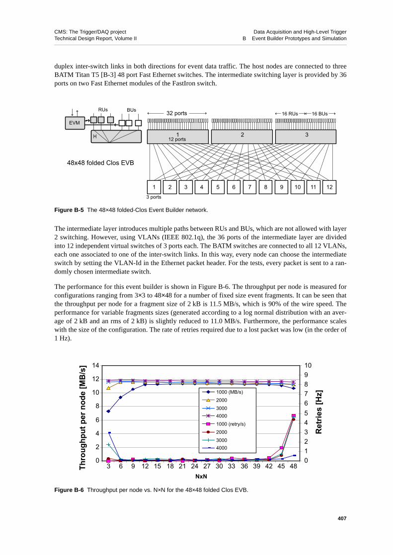
CMS: The Trigger/DAQ project Data Acquisition and High-Level TriggerTechnical Design Report, Volume II B Event Builder Prototypes and Simulation
duplex inter-switch links in both directions for event data traffic. The host nodes are connected to threeBATM Titan T5 [B-3] 48 port Fast Ethernet switches. The intermediate switching layer is provided by 36ports on two Fast Ethernet modules of the FastIron switch.
The intermediate layer introduces multiple paths between RUs and BUs, which are not allowed with layer2 switching. However, using VLANs (IEEE 802.1q), the 36 ports of the intermediate layer are dividedinto 12 independent virtual switches of 3 ports each. The BATM switches are connected to all 12 VLANs,each one associated to one of the inter-switch links. In this way, every node can choose the intermediateswitch by setting the VLAN-Id in the Ethernet packet header. For the tests, every packet is sent to a ran-domly chosen intermediate switch.
The performance for this event builder is shown in Figure B-6. The throughput per node is measured forconfigurations ranging from 3×3 to 48×48 for a number of fixed size event fragments. It can be seen thatthe throughput per node for a fragment size of 2 kB is 11.5 MB/s, which is 90% of the wire speed. Theperformance for variable fragments sizes (generated according to a log normal distribution with an aver-age of 2 kB and an rms of 2 kB) is slightly reduced to 11.0 MB/s. Furthermore, the performance scaleswith the size of the configuration. The rate of retries required due to a lost packet was low (in the order of1 Hz).
Figure B-5 The 48×48 folded-Clos Event Builder network.
Figure B-6 Throughput per node vs. N×N for the 48×48 folded Clos EVB.
1 2
32 ports
12 ports
3 ports
3 4 5 6 7 8 9 10 11 12
16 RUs
EVM
RUs BUs
1 2 3
16 BUs
48x48 folded Clos EVB
0
2
4
6
8
10
12
14
3 6 9 12 15 18 21 24 27 30 33 36 39 42 45 48NxN
Thro
ughp
ut p
er n
ode
[MB/
s]
012345678910
Ret
ries
[Hz]1000 (MB/s)
2000300040001000 (retry/s)200030004000
407

CMS: The Trigger/DAQ project Data Acquisition and High-Level TriggerTechnical Design Report, Volume II B Event Builder Prototypes and Simulation
The conclusion is that it is possible to construct composite switching networks for Layer-2 frame switch-ing out of smaller switches if they support VLANs. It also seems possible to achieve high efficiency,when using such networks for event building. More studies are however needed to verify that this holdsalso for Gigabit Ethernet, rather than FastEthernet.
B.3 Gigabit Ethernet TCP/IP Test-benches
This section presents the results of event building using TCP/IP over Gigabit Ethernet. Using TCP/IPrather than Layer-2 frames has a number of advantages. Foremost, it provides a reliable transport servicethat removes the need for the event building application to detect and deal with lost packets. TCP/IP alsoprovides flow control and congestion control. Flow control tries to avoid buffer overruns at end points,whereas congestion control tries to prevent packet loss in intermediate nodes (switches or routers). Be-sides these technical merits, TCP/IP also provides a solution based on standard software. HoweverTCP/IP is more demanding on host resources and the scaling properties for event builder traffic at highload are still unknown.
B.3.1 Point-to-point Streaming Tests
TCP/IP performance is highly dependent on NIC and host CPU performance and on the TCP/IP protocolstack implementation of the host-OS. The TCP/IP performance has been measured for a number of differ-ent NICs and hosts. One-way streaming tests were performed on host PCs running Linux 2.4. One hostrepeatedly sent fixed sized messages whilst another received them.
The PCs are based on the Supermicro 370DLE motherboard with a 64b/66MHz PCI-bus, equipped with a1 GHz Pentium-III CPU. The Ethernet frames are of the standard size (MTU=1500). The standard TCPoptions were used, except for the sizes of the send and receive socket buffers which were set to 256 kB.Note, that by default TCP uses the Nagle algorithm which can combine several TCP segments into apacket, to increase efficiency but at the cost of latency. The one-way streaming throughput is shown inFigure B-7 as a function of the message size. It can be seen that there is a significant variation in the per-formance between the NICs. The AceNIC[B-4] reaches a maximum throughput of about 88 MB/s for siz-es above 800 B (70% of the link bandwidth), whereas the RM674TX1 [B-5] NIC reaches about 115 MB/sfor sizes above 2 kB (92% of the link bandwidth).
The tests were repeated with the NICs configured to use Jumbo frames (MTU=9000). These results arecompared with those obtained with standard frame sizes in Figure B-8. A significant improvement can beobserved.
Further point-to-point tests were performed with a two-rail system based on two AceNIC NICs per PC.The 1 GHz Pentium-III based PC used in the tests above was found not to be powerful enough to drivethe two links close to the link bandwidth2. However, with a 2 GHz Pentium-IV Xeon based PC, an aggre-gate throughput of about 247 MB/s was reached using jumbo frames. Measurements with this platformare presented in Figure B-9. Here the two-rail configuration is compared with the one-rail, both for stand-ard and Jumbo frames. Similar performance has been obtained with NICs based on the family of Intel8254xx Ethernet controllers.
1. The RM674TX is based on the Intel 82544 Ethernet controller.
2. This corresponds to the empirical rule that 1 Hz of CPU is required per bps transmitted.
408

CMS: The Trigger/DAQ project Data Acquisition and High-Level TriggerTechnical Design Report, Volume II B Event Builder Prototypes and Simulation
B.3.2 Event Building Tests
The TCP/IP option has been evaluated using the same test-bench (see Section 6.5.2.3, "Test-bench Re-sults for Layer-2 Frames") as was used for the studies of the event building with Ethernet Layer-2 frames.Briefly, it comprises 64 Pentium-III based PCs (750 MHz or 1 GHz) with AceNIC NICs connected to aFastIron-8000 switch. The switch model used does not support Jumbo frames. Therefore, the presentstudies are restricted to standard frames. The trigger is not emulated and the throughput measured corre-sponds to the saturation limit.
The application software running on the PCs implements the event building protocol discussed inSection 5.3.2.1, "Event Flow Protocols", using TCP socket connections to transmit data. Each instance ofthe RU, BU or BM application runs as a single process on its host. The select mechanism is used for the
Figure B-7 Streaming TCP/IP performance for various NICs (AceNIC[B-4], RM674TX[B-5], SK9821[B-2], Net-gear[B-6]). Hosts are used based on 1 GHz Intel Pentium-III CPUs and Ethernet frames of standard size(MTU=1500).
Figure B-8 Streaming TCP/IP performance for Jumbo frames compared to standard frames. Hosts with 1 GHzIntel Pentium-III CPUs are used.
Thro
ughp
ut [
MB
/s]
0
20
40
60
80
100
120
100 1000 10000 100000
Message Size [Bytes]
link BW (1Gbps)RM674TXAceNICNetgearSK-9821
Thro
ughp
ut [
MB
/s]
0
20
40
60
80
100
120
140
100 1000 10000 100000
Message Size [Bytes]
link BW (1Gbps)RM674TX - MTU=9000RM674TX AceNIC - MTU=9000AceNIC
409

CMS: The Trigger/DAQ project Data Acquisition and High-Level TriggerTechnical Design Report, Volume II B Event Builder Prototypes and Simulation
synchronous I/O multiplexing to send and receive data via the socket connections to all remote applica-tions participating in the event building.
The control messages are bundled for efficiency reasons. The request messages from BU to RU and theallocation or clear messages between BU and BM aggregate 8 and 16 logical messages, respectively. Fur-thermore, each BU builds 64 events concurrently.
B.3.2.1 1×1 EVB
As a first step, tests have been done with a simpler configuration based on just two nodes; one RU andone BU. These are connected directly, i.e. without a switch between them. This 1×1 Event Builder doesnot include a BM. The function of the BM to allocate events to BUs is anyhow not needed, as there isonly a single BU.
The throughput per node versus fragment size is shown in Figure B-10, and is compared to the one-waystreaming throughput discussed in the previous section. Results are given, both for normal and Jumboframes. It can be seen that the event builder throughput is significantly lower than to the one-way stream-ing throughput. This holds in particular for smaller fragment sizes. It should be noted that the event build-ing application is more complex, because communication is full duplex and the receiving of messages hasto be done in at least two steps1. The throughput per node at a size of 16 kB is about 76 MB/s for standardframes and 95 MB/s for Jumbo frames.
B.3.2.2 31×31 EVB with BM
Studies were done with the 31×31 EVB configuration, including a BM. The throughput per node as afunction of the fragment size is shown in Figure B-11. For a size of 16 kB the achieved throughput pernode is about 75 MB/s. This throughput corresponds to 85% of the measured one-way streaming through-put (88 MB/s). It should be noted that due to this limitation of the host and/or NIC, the switch load is onlyabout 60%.
Figure B-9 Streaming TCP/IP performance for a two-rail compared to one-rail configuration with standard andJumbo frames. The NIC used is AceNIC. Hosts with 2 GHz Pentium-IV Xeon CPUs are used.
1. the header including the size of the message must be read before the variable sized message body
0
50
100
150
200
250
100 1000 10000 100000
Thro
ughp
ut [
MB
/s]
Message Size [Bytes]
link BW (1Gbps)AceNIC 2-rail MTU=9000AceNIC 2-rail MTU=1500
AceNIC 1-rail MTU=9000AceNIC 1-rail MTU=1500
410

CMS: The Trigger/DAQ project Data Acquisition and High-Level TriggerTechnical Design Report, Volume II B Event Builder Prototypes and Simulation
The size of the Event Builder is varied from 3x3 to 31x31 in Figure B-12 for the nominal case of variablesize fragments with an average of 16 kB and an rms of 8 kB. It can be seen that the throughput per nodescales approximately with the size of the configuration and a value of about 75 MB/s is achieved.
Figure B-10 Throughput per node vs. fragment size for a TCP/IP 1×1 EVB. The vertical dotted line indicates afragment size of 16 kB.
Figure B-11 Throughput per node vs. fragment size for a TCP/IP 31×31 EVB with BM.
0
20
40
60
80
120
100
140
100 1000 10000 100000Fragment Size [Bytes]
link BW (1Gbps)TCP 1-way stream MTU=9000TCP 1-way stream MTU=1500TCP EVB 1x1 MTU=1500TCP EVB 1x1 MTU=9000
Thro
ughp
ut p
er n
ode
[MB
/s]
Thro
ughp
ut p
er n
ode
[MB
/s]
Fragment Size [Bytes]
0
20
40
60
80
100
120
140
100 1000 10000 100000
link BW (1Gbps)TCP/IP EVB 31x31+BM
411

CMS: The Trigger/DAQ project Data Acquisition and High-Level TriggerTechnical Design Report, Volume II B Event Builder Prototypes and Simulation
B.4 Simulation of Myrinet Event Builder
A successful simulation of the EVB is one that aids the understanding of the system’s functions and alsopredicts convincingly the behaviour of the system in different contexts and with different parameters.Given that a full prototype of the final system cannot be built due to the resources currently available animportant element provided by simulation is the expected behaviour of the full final system once all thecomponents are combined.
In what follows, after a short introduction to the simulation package, an overview of the modelling of sin-gle EVB components and EVB networks is given. Data and simulation results are compared and a fore-cast of the EVB performance with LANai10 based hardware is made. A forecast for a full sized RUBuilder and FED Builder is presented in Section 6.7.1.
B.4.1 Simulation Package
The Ptolemy package [B-7], developed at the University of California at Berkeley, provides a frameworkfor the simulation of complex and heterogeneous systems. For the implementation of the EVB simulationthe discrete event (DE) domain was used. The DE domain in Ptolemy is designed for time-oriented simu-lations of systems such as communication networks. Actions are described as the exchange of “Particles”between objects. These objects, called “stars” in the Ptolemy terminology, can receive Particles over oneor many ports and trigger the emission of new Particles. Stars represent functional units like the ReadoutUnit or the Builder Unit.
The Ptolemy environment provides a hierarchical organization of all its objects. As an example, stars canbe grouped together into “galaxies”, and these galaxies can communicate with other galaxies or withstars. Proceeding further, one can define a universe as a combination of stars and galaxies with no exter-nal ports. A universe represents a complete simulation model. In the case of the Event Builder model de-scribed later, it is made of a single galaxy by interconnecting ports from different stars.
Figure B-12 Throughput per node vs. N×N for a TCP/IP EVB. The fragment sizes are generated according to alog-normal distribution with an average of 16 kB and an rms of 8 kB.
Thro
ughp
ut p
er n
ode
[MB
/s]
0
20
20
40
60
80
100
120
140
0 5 10 15 25 30
N for NxN EVB
link BW (1Gbps)TCP EVB NxN+BM frag size = 16 kB, rms = 8 kB
412

CMS: The Trigger/DAQ project Data Acquisition and High-Level TriggerTechnical Design Report, Volume II B Event Builder Prototypes and Simulation
Ptolemy has been developed in C++ using object-oriented software which supports extensibility andmodularity. Extensions to existing stars and creation of new stars can thus be accomplished easily withthe aid of various objects and classes provided by Ptolemy. The analysis package ROOT [B-8] has beenadded for data analysis and for automatic job submission. It allows also to resolve the EVB traffic on thesingle packet scale. To reduce processing times, a front-end is being developed to utilize a computer farmand run multiple simulations in parallel.
In the EVB simulation within the DE domain, a Particle represents an event that corresponds to a changeof the system state. Events can be network messages, DMA transfers, busy states etc. The DE schedulerprocesses events in chronological order. Each particle has an associated time stamp which is generated bythe birth-giving star based on the input event that triggered the generation and the latency of the action.
In the simulation, the EVB is resolved into functional units implemented as stars which will be describedin detail in the following sections. The EVB communication protocol of the different units is implement-ed as it is used in the real EVB system, as described in Chapter 4.
B.4.2 Simulation of EVB Components
An overview of the EVB components that have been implemented is given in Table B-3. Either the FEDBuilder or the RU Builder can currently be simulated. FED and RU Builder combined in a single systemhave not been simulated. Since the RU will have sufficient memory to be decoupled from statistical fluc-tuations of the FED Builder the full system’s performance is governed by the least performant componentof the FED Builder / RU Builder system. Figure B-13 shows a schematic of the structure of the simulationwith its components and the relation between them.
B.4.2.1 Data Sources
The data chain begins with the RU or FRL respectively. Components in the readout chain prior to theRU/FRL are not implemented. The data source is modelled with a random generator of fragment sizes,the probability distribution can be freely chosen and different for each RU/FRL. Predefined analyticalfunctions (boxcar, normal, log-normal as defined in Table B-4) or histograms can be used to define theprobability density function (pdf).
The flexible design of the data source allows to study various scenarios of data conditions. It is also pos-sible to vary the correlation of fragment sizes between data sources from 0% to 100%. The correlation isdefined as the linear correlation coefficient r:
, with , x and y being fragment sizes of a pair of data sources.
Besides correlation, other aspects of the study of data conditions were unbalanced fragment sizes andpathologically large fragments. The imbalance of input was parametrized with the imbalance ratio R de-fined as R = Lmax / Lmin , with Lmax the maximum average fragment size and Lmin the minimum averagefragment size of an ensemble of data inputs.
Table B-3 Overview of data sources and sinks in the simulation.
Schema Source Sink Other
FED Builder FRL RUI Trigger
RU Builder RU BU EVM
SSSr yyxxxy /= ∑ −−= ))(( yyxxS xy
413
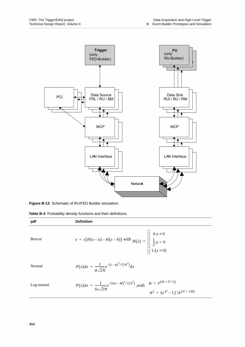
CMS: The Trigger/DAQ project Data Acquisition and High-Level TriggerTechnical Design Report, Volume II B Event Builder Prototypes and Simulation
Figure B-13 Schematic of RU/FED Builder simulation.
Table B-4 Probability density functions and their definitions.
pdf Definition
Boxcar with
Normal
Log-normal ,with
LA
MCP
Data Sink
FU(only RU-Builder)
Data Source
MCP
LA
PCIData Source
MCP
LA
PCI
Network
Data SourceFRL / RU / BM
Trigger(only FED-Builder)
MCP
LAN Interface
PCI
LA
MCP
Data Sink
FU(only RU-Builder)
LAN Interface
MCP
Data SinkRUI / BU / RM
FU(only RU-Builder)
y c H x a–( ) H x b–( )–[ ]= H x( )
0 x; 0<12--- x 0=;
1 x 0>( );
=
P x( )dx1
σ 2π--------------e
x µ–( )22σ2( )⁄–
dx=
µ e M S2 2⁄+( )=P x( )dx
1
Sx 2π-----------------e
x M–ln( )22S
2( )⁄–=
σ2 e( S2 1– ) e⋅ S2 2M+( )=
414

CMS: The Trigger/DAQ project Data Acquisition and High-Level TriggerTechnical Design Report, Volume II B Event Builder Prototypes and Simulation
Pathologically large fragments, or “jumbo fragments”, where simulated by injecting a single large frag-ment, with a size of 200 kB, at a defined time into one data source and observe the behaviour of the sys-tem.
B.4.2.2 FRL Model (FED Builder)
The FRL represents the first element in the data flow of the FED Builder simulation. The FED level is im-plicit in the data source and the merging of FEDs can be emulated by providing adequate fragment sizedistributions. The PCI bus is modelled with priority queues and arbitration for different access modes,and comprises detailed timings for set-ups and transmission of data. The interface to the network is donewith the NIC model described in Appendix B.4.2.9. No network traffic shaping is done in the FED Build-er case, but maximal transfer units (MTU) can be employed.
The FRL is connected to a trigger (described in Appendix B.4.2.4) and can throttle in case it is not capa-ble of keeping up with the trigger rate. Analogous to the real system the memory is limited and is settablewith a parameter.
B.4.2.3 RUI Model (FED Builder)
The RUI is collecting the data fragments created by the FRLs. It assembles super-fragments and forwardsthem to the RUs. The collecting of fragments and the assembling of the super-fragments are modelled inthe simulation. The RUI is implemented without a detailed modelling of the PCI bus and it is assumedthat forwarding of the super-fragments to the RUs is negligible compared to the time needed to collectfragments. The RUI model is used to study the performance of super-fragment building and the memoryusage.
B.4.2.4 Trigger Model (FED Builder)
The trigger model in the simulation is a simple object which emits trigger signals with a Poisson time dis-tribution with adjustable mean. The trigger can be throttled by external objects and monitors the efficien-cy. The trigger efficiency is defined as ε=Nacp/Ntotwith Nacp the number of issued trigger signals in theunthrottled state and Ntot the total number of trigger events.
The trigger is a global module which connects to all FED Builders in case of multiple FED Builders.
B.4.2.5 RU Model (RU Builder)
The RU model features similar components as the FRL. It includes the PCI model and the NIC model, butit does not connect to a trigger. The data source is modelled in the same way as in the FRL. Since su-per-fragments are injected independently of the trigger, it is assumed that the FED Builder, i.e. RUI, satu-rates the RU. Limitations in the performance of the RU Builder are thus not caused by the FED Builder,but by genuine RU properties and represent the saturation limit.
The forwarding of super-fragments to the network is done via the NIC. The same protocol as in the realhardware has been implemented. The packing of super-fragments into MTUs and the Barrel Shifter proto-col are driven by the NIC.
The event building protocol has been implemented. The RU can operate with and without EVM1. Studieswithout EVM have been useful to verify the simulation with data obtained from the test-bench.
415

CMS: The Trigger/DAQ project Data Acquisition and High-Level TriggerTechnical Design Report, Volume II B Event Builder Prototypes and Simulation
B.4.2.6 BU Model (RU Builder)
Similar to the RUI model the PCI bus is not included in the simulation of the BU. It is assumed that thetransmission time of super-fragments from the RU to the BU will be long compared to the transmission ofsuper-fragments from the receiving NIC to the BU and that the PCI will not severely limit the transmis-sion of control messages.
The BU can be operated with and without EVM. When the EVM is absent, the BU will act as a pure sink.As for the RU the full event building protocol has been implemented. Optionally the assembly and ship-ping of complete events to the FUs can be invoked. The resources and the packing factor of control mes-sages in the BU are configurable.
B.4.2.7 EVM Model (RU Builder)
The EVM model consists of an RM, BM, trigger and an RCN. The RM associates Event_IDs with triggerevents and distributes the information to the RUs. The RM maps each trigger to an available Event_IDand sends the information with minimal latency to all RUs. The BM serves newly allocated Event IDs toBUs according to their requests. An allocated Event ID becomes available again as soon as it is releasedby the BU. The RCN can be implemented as a separate network, but by default the Myrinet RU Builderswitch is used. In a configuration with EVM the RM is connected to the BU side and the BM to the RUside.
The EVM is configurable. Parameters include the event table size, packing factor of control messages,RCN bandwidth and trigger rates.
B.4.2.8 FU Model (RU Builder)
The FUs are modelled as a simple extension to the BU in case an EVM is present. The FUs are connectedto the BU over an idealized network. Each FU has settable processing time distributions and memorysize. Typically eight FUs were connected to one BU.
B.4.2.9 NIC Model
Before data can be send to or received from the network they have to be copied from the host memoryinto the memory of the NIC or vice versa. Thus, the NIC model is included in all models which are con-nected to the Myrinet network: FRL, RUI, RU, BU and EVM.
The copy process uses both DMA and programmed I/O modes to transfer data via the PCI bus. The laten-cy of the transfer process is modelled in detail taking into account the finite memory bandwidth of thePCI bus, its usage, and processing times. In case of the RUI and the BU models, the communication be-tween NIC and RUI/BU is processed directly, bypassing the DMA and Programmed I/O modelling.
The NIC is modelled with two stars, the MCP star and the Network Interface (NI) star. The physical trans-port and first protocol layer are restricted to Myrinet networks in the simulation. The MCP star modelsthe custom firmware running on the RISC processor in the NIC and the NI star simulates the actual hard-ware interfacing to the network. The latencies introduced by the NIC are given by the processing timesfor distinct tasks. These processing times are given as parameters to the NIC star and have been deter-
1. In this case the Event ID allocation is done by the BU itself, using a static algorithm.
416

CMS: The Trigger/DAQ project Data Acquisition and High-Level TriggerTechnical Design Report, Volume II B Event Builder Prototypes and Simulation
mined from test-bench set-ups. Thus the simulation requires no “free” parameters, beyond those obtaina-ble from point-to-point measurements.
The NIC model can simulate LANai9 and LANai10 hardware, the difference being that LANai9 has one2 Gb/s port whereas LANai10 will provide two 2 Gb/s ports and will allow higher processing speeds rel-ative to LANai9 hardware due to faster memory, a faster processor and an improved DMA architecture.Since the LANai10 is not yet available, the anticipated performance has been estimated by reducing theprocessing times by a factor two and adding a second port in the simulation.
B.4.2.10 Single Switch Elements
Implementations of single crossbar switch elements with 8 ports and 16 ports have been made by others[B-9], corresponding to Myrinet Xbar8 and Xbar16 switches. A round robin token arbitration scheme hasbeen added. The implementation follows closely the Myrinet network technology using wormhole rout-ing, back-pressure flow control and small slack buffers as described in detail in Appendix A.2.1.
B.4.3 FED Builder Simulation
The FED Builder is the first stage of the event building process. Fragments are supplied by one or twoFEDs to one FRL and the data of eight FRLs are assembled into a super-fragment in a RUI. The simula-tion integrates the data source in the FRL-model, which allows to study the dependency of the perform-ance on various data conditions.
The interconnect between FRLs and RUIs is formed by one or two 16 ports crossbar switches for LANai9and LANai10 hardware, respectively. Hence in the LANai10 case, two independent rails are available.The FRL and RUI models connect via the NIC model to the network. The trigger model is employed toprovide trigger signals to the FRL model. The FRL can throttle the trigger if the rate is exceeding its ca-pacity.
The FED Builder operates in a pure push manner, incoming fragments on the FRL side are pushed to theirdestination on the RUI side and no traffic shaping as in the case of the RU Builder is employed. Theswitch utilization can be improved dividing fragments into packets of a maximum size (MTU), so largefragments get divided into multiple smaller packets. This reduces the effect of output port blocking bylarge fragments, since other senders can deliver their packets interleaved and continue with the next desti-nation.
The throughput of a simulated LANai9 FED Builder without MTUs for different distribution types iscompared to test-bench data in Figure B-14. The distributions differ in width, while the mean is fixed to2 kB and the pdf is a log-normal. In general a good agreement between data and simulation is observed.
Starting from the good description of the current test-bench hardware different scenarios where simulatedto investigate the influence of data conditions, the performance of LANai10 hardware, and the usage ofMTUs. The fundamental “figure-of-merit” is the maximal trigger rate the FED Builder can accept withoutthrottling the trigger.
The trigger efficiency was scanned for different trigger rates to establish, that the maximal trigger rate isdetermined by the saturation throughput divided by the average fragment size. The result is shown inFigure B-15 for LANai9 and LANai10 hardware with and without the usage of MTU and a log-normalfragment size distribution with a mean of 2 kB and an rms of 2 kB. The trigger efficiency starts to degrade
417
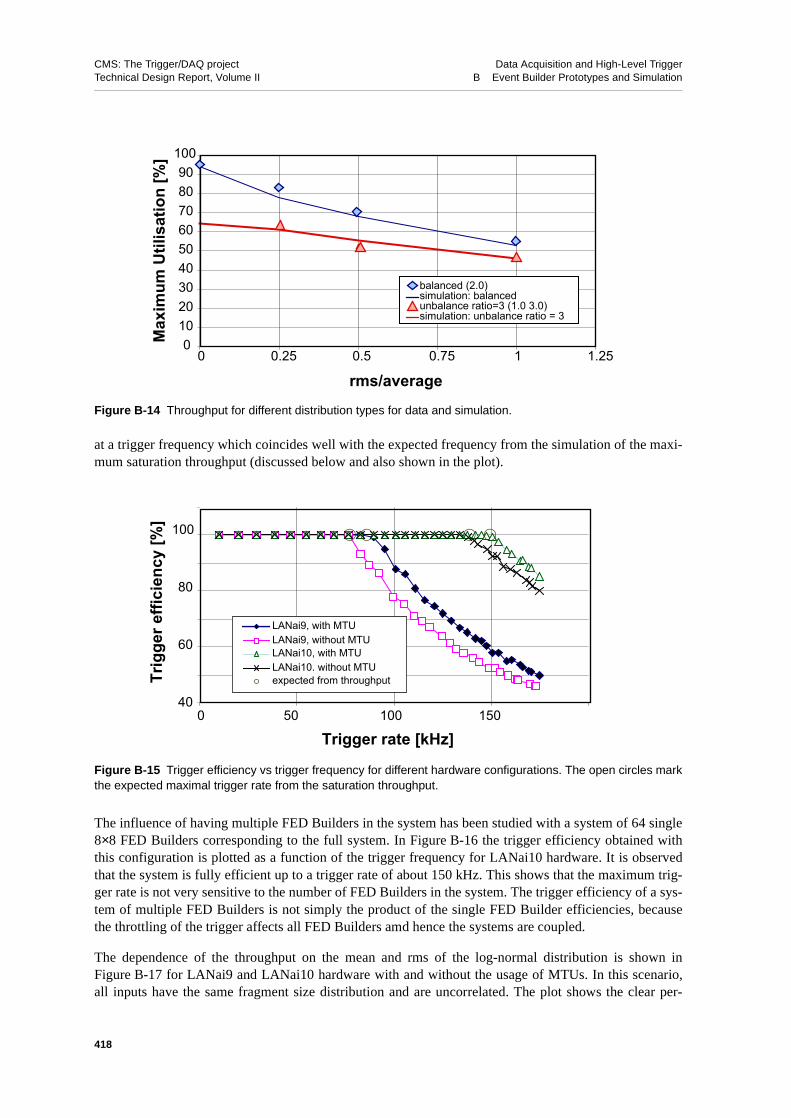
CMS: The Trigger/DAQ project Data Acquisition and High-Level TriggerTechnical Design Report, Volume II B Event Builder Prototypes and Simulation
at a trigger frequency which coincides well with the expected frequency from the simulation of the maxi-mum saturation throughput (discussed below and also shown in the plot).
The influence of having multiple FED Builders in the system has been studied with a system of 64 single8×8 FED Builders corresponding to the full system. In Figure B-16 the trigger efficiency obtained withthis configuration is plotted as a function of the trigger frequency for LANai10 hardware. It is observedthat the system is fully efficient up to a trigger rate of about 150 kHz. This shows that the maximum trig-ger rate is not very sensitive to the number of FED Builders in the system. The trigger efficiency of a sys-tem of multiple FED Builders is not simply the product of the single FED Builder efficiencies, becausethe throttling of the trigger affects all FED Builders amd hence the systems are coupled.
The dependence of the throughput on the mean and rms of the log-normal distribution is shown inFigure B-17 for LANai9 and LANai10 hardware with and without the usage of MTUs. In this scenario,all inputs have the same fragment size distribution and are uncorrelated. The plot shows the clear per-
Figure B-14 Throughput for different distribution types for data and simulation.
Figure B-15 Trigger efficiency vs trigger frequency for different hardware configurations. The open circles markthe expected maximal trigger rate from the saturation throughput.
0102030405060708090
100
0 0.25 0.5 0.75 1 1.25
rms/average
Max
imum
Util
isat
ion
[%]
balanced (2.0)simulation: balancedunbalance ratio=3 (1.0 3.0)simulation: unbalance ratio = 3
40
60
80
100
0 50 100 150
Trigger rate [kHz]
Trig
ger e
ffici
ency
[%]
LANai9, with MTULANai9, without MTULANai10, with MTULANai10. without MTUexpected from throughput
418

CMS: The Trigger/DAQ project Data Acquisition and High-Level TriggerTechnical Design Report, Volume II B Event Builder Prototypes and Simulation
formance gain when the two-rail LANai10 hardware is employed, and also demonstrates the beneficialeffect of using MTUs.
The performance of the FED Builder is sensitive to the fragment size distributions of the FRL. The casewhere a set of FRLs send more data on average than the rest of the FRLs was studied by varying the im-balance parameter for a configuration with 4 FRLs above and 4 below the average (4-4), and another con-figuration with 1 above and 7 below the average (1-7). The result for LANai9 and LANai10 hardwarewith and without MTU is shown in Figure B-18.
For LANai10 hardware, the target throughput of 200 MB/s is sustained for the “4-4” configuration up toR values of 3.5, while for the “1-7” configuration the limit is reached at R=1.9. Although the “1-7” con-figuration seems to be more sensitive to R, it should be noted that in terms of the actual maximum aver-
Figure B-16 Trigger efficiency vs. trigger rate for 64 8×8 FED Builders and a log-normal fragment size distribu-tion with a mean of 2 kB and a rms of 2 kB.
Figure B-17 Dependence of the throughput per node on the mean and RMS of the input distribution to theFRLs. The rms is is set equal to the mean of the log-normal distribution.
60
0
80
100
0 50 100 150
Trigger rate [kHz]
Trig
ger e
ffici
ency
[%]
0
50100
150
200
250
300
350
10 100 1000 10000
Average fragment size, rms [Bytes]
Thro
ughp
ut p
er n
ode
[MB
/s]
LANai10, with MTULANai10, w/o MTULANai9, with MTULANai9, w/o MTU
419

CMS: The Trigger/DAQ project Data Acquisition and High-Level TriggerTechnical Design Report, Volume II B Event Builder Prototypes and Simulation
age fragment size the values do not differ by much, namely 3.1 kB for the “4-4” configuration and 3.4 kBfor the “1-7” configuration.
The correlation of fragment sizes between different FRLs is very likely to occur, since the data volume ofmany detector components is determined by the multiplicity of the underlying minimum bias events. Thesensitivity of the FED Builder performance has been studied by varying the linear correlation coefficientbetween the FRL data sources for a log-normal distribution with an average of 2 kB and an rms of 2 kB.The results for LANai9 and LANai10 hardware with and without MTU is shown in Figure B-19. The cor-relation of fragment sizes has a negligible influence on the performance over the full range of the correla-tion coefficient r.
The behaviour of the FED Builder has been studied for the special case that one FRL sends a very largefragment, so called “jumbo fragment”. The FRL will have enough memory (1 MB) to buffer and send this“jumbo fragment”. However, the input port of the RUI will not be accessible by the other FRLs during thetransmission of the jumbo fragment and thus a serious degradation of performance might occur if the oth-er FRLs are stalled and have to wait for the input to the specific RUI to become available. The “jumbofragment” scenario was studied for a one rail LANai9 and a two rail LANai10 network with and without
Figure B-18 Throughput vs. the imbalance parameter R, shown for LANai9 and LANai10 hardware with andwithout usage of MTUs for both 4-4 and 1-7 scenarios.
Thro
ughp
ut p
er n
ode
[MB
/s]
0
50
100
150
200
250
300
1 2 3 4 5 6
Imbalance ratio R
LANai10 4-4LANai10 1-7LANai9 4-4LANai9 1-7
a) with Maximal Transfer Unit (MTU)
0
50
100
150
200
250
300
1 2 3 4 5 6
Imbalance ratio R
Thro
ughp
ut p
er n
ode
[MB
/s] LANai10 4-4
LANai10 1-7LANai9 4-4LANai9 1-7
b) without Maximal Transfer Unit (MTU)
420

CMS: The Trigger/DAQ project Data Acquisition and High-Level TriggerTechnical Design Report, Volume II B Event Builder Prototypes and Simulation
usage of MTU. The size of the “jumbo fragment” was set to 200 kB. The average throughput of all FRLnodes as a function of time is monitored. The injection time of the “jumbo fragment” is at t = 10 ms in theFRL. The fragment has to be transported to the NIC memory and is buffered there until it is sent off to thenetwork. The storage period in the NIC depends on the NIC memory size and utilization, and on the drainspeed. The time the fragment needs from the creation in the FRL until it reaches the network is of the or-der of 5ms for a one-rail LANai9 builder and only 2.5 ms for a two-rail LANai10 builder since the latterprovides roughly twice the bandwidth of the former.
The behaviour of the throughput is shown in Figure B-20 for LANai9 and LANai10 hardware, with andwithout MTUs. A substantial degradation of throughput is seen only for LANai9 hardware in the case thatno MTUs are used (Figure B-20 a)). At transmission time (t=14ms) the throughput for the nodes nottransmitting the “jumbo fragment” drops to zero, while one node (full circle) uses the switch exclusively.If MTUs are used, the switch output port is no longer blocked by one large fragment but other fragmentscan interleave (Figure B-20 b)). The behaviour is not critical for LANai10 even in the case without MTU.Here, the second rail prevents a blocking of the output ports (Figure B-20 c)). The nodes not transmittingthe “jumbo fragment” can still use half of the bandwidth of the FED Builder, while the node with the“jumbo fragment” uses one link exclusively and the second one for fragments of “normal” size.
A microscopic view of the incident is shown in Figure B-21 for LANai9 and LANai10 hardware. The plotfocuses on the FRL which produces the “jumbo fragment”. Here the event numbers in the system areplotted versus the time of creation in the FRL. The dots correspond to the creation of an event fragmentassociated to an event number in the FRL. The network is blocked without the employment of MTUs.Only one fragment, the jumbo fragment, is being transmitted through the switch. No other fragments arebeing received, which can be seen by the absence of points during the super-fragment transmission timeat around 14ms for LANai9 hardware. If MTUs are used, the super-fragment is no longer exclusively us-ing one output link, but the segmentation allows other senders to deliver their packets. This is shown inthe plot, where the dots with constant event number are the MTUs belonging to the “jumbo fragment” (att=10ms) being created in the FRL, while the other dots clearly show the progression of the FED Buildertraffic even during the transmission time at about t=14ms.
Figure B-19 Throughput vs. correlation coefficient between the FRL data sources for a log-normal distributionwith 2 kB mean and 2 kB rms.
0
50
100
150
200
250
300
350
0 0.2 0.4 0.6 0.8 1
Correlation r
Thro
ughp
ut p
er n
ode
[MB/
s]
LANai10 with MTULANai10 without MTULANai9 with MTULANai9 without MTU
421

CMS: The Trigger/DAQ project Data Acquisition and High-Level TriggerTechnical Design Report, Volume II B Event Builder Prototypes and Simulation
a) LANai9, no MTU b) LANai9, with MTU
c) LANai10, no MTU d) LANai10, with MTU
Figure B-20 Throughput per node as a function of time for 8 FRL nodes. A “jumbo fragment” is injected att=10ms and propagates to the network at about t = 15ms (LANai9) and t = 12.5ms (LANai10). The full circlesshow the throughput of the FRL node with the “jumbo fragment”, the empty circles show the 7 other FRL nodes.
Figure B-21 Event numbers in the system vs. time. A “jumbo fragment” is injected at t=10 ms.
Time [mus]
10000 12000 14000 16000 18000 20000
Thro
ughp
ut p
er n
ode
[MB
/s]
0
50
100
150
200
250
0
20
40
60
80
100
120
140
160
180
200
220
Time [mus]
10000 12000 14000 16000 18000 20000
Thro
ughp
ut p
er n
ode
[MB
/s]
Time [mus]
10000 12000 14000 16000 18000 20000
Thro
ughp
ut p
er n
ode
[MB
/s]
0
50
100
150
200
250
300
350
400
Time [mus]
10000 12000 14000 16000 18000 20000
Thro
ughp
ut p
er n
ode
[MB
/s]
0
50
100
150
200
250
300
350
400
1000
1200
1400
1600
1800
2000
2200
10000 11000 12000 13000 14000 15000 16000
Time [ µs]
Even
t ID
LANai10, with MTULANai10, no MTULANai9, with MTULANai9, no MTU
422

CMS: The Trigger/DAQ project Data Acquisition and High-Level TriggerTechnical Design Report, Volume II B Event Builder Prototypes and Simulation
B.4.4 RU Builder Simulation
The scope of the RU Builder simulation is to verify results obtained with test-bench set-ups and to predicton the basis of the reliable description of the test-bench data the performance of the final system withLANai10 hardware.
The simulation of the RU Builder closely follows the set-up of the test-benches (see Chapter 6.5, "RUBuilder") as well as the layout proposed for the final system (see Chapter 4.3, "RU Builder"), which in-cludes the EVM. The FED Builder has not been included in the simulation of the RU Builder. The datasource is integrated into the RU model. As explained above, the coupling between both builders is low, sothat each subsystem can be studied independently of the other as it was done with the test-benches.
Extensive studies of the throughput dependence on the fragment size allowed to verify the detailed modelof the hardware in the simulation. Especially the preparation of packets in the NIC, which has to keep upwith the barrel shifter cycle, is a time critical process since it puts the NIC to the limit of its processingpower and internal memory bandwidth. A detailed description of the internals of the NIC can be found inChapter A.2, "Myrinet Technology and Products".
Special attention has been paid to reproduce the measurement which can be seen as a benchmark test forthe simulation. The result is shown in Figure B-22 where the simulation results are compared with thedata obtained from the test-bench operating with 32 RUs and 32 BUs, and no EVM present. In the casethat no EVM is present it is assumed that the BUs will always have allocated Event_IDs available. Thetwo simulation curves differ in the assumptions of the memory bandwidth internally available to the NICprocessor. If multiple DMAs are executed, the remaining memory bandwidth available can limit the exe-cution time of the program running on the NIC processor. To model this, the processing times were in-creased depending on the number of ongoing DMAs. The lower curve implements this “memorychoking” effect, while the upper curve assumes that sufficient bandwidth is available. The data points be-low a fragment size of 2 kB and above 6 kB are well described by the simulation without memory chok-ing, while the data points in between are better described by the model with “memory choking”. Since thedata-points are enclosed in between the two bands, the bands can be seen as the level of uncertainty in thesimulation. The operation point of the RU Builder will be at 16 kB corresponding to the average size of asuper-fragment, where the influence of the memory choking is insignificant.
Figure B-22 Throughput per node as a function of the fragment size for a 32×32 network and LANai9 hard-ware. The bands represent the simulation result for two different performance assumptions. The symbols showthe data points obtained with the prototype.
0
50
100
150
200
250
300
10 1000 100000
Fragment size [Bytes]
Thro
ughp
ut p
er n
ode
[MB
/s]
DataSimulation 1Simulation 2
423

CMS: The Trigger/DAQ project Data Acquisition and High-Level TriggerTechnical Design Report, Volume II B Event Builder Prototypes and Simulation
The final system will have an EVM with an RM on the BU side and an BM on the RU side. The effect ofthe addition of an EVM has been studied. The EVM model is described in Chapter B.4.2.7, "EVM Model(RU Builder)". The addition is expected to affect the performance of the RU Builder since firstly one portof the builder is used for the EVM, and, secondly, the distribution of Event_ID, or rather a shortage ofthem, can delay the sending of fragments and thus degrade the performance. The first cause of degrada-tion is inherent to the design and irreducible. The effect of the second cause is dependent on the numberof available resources and the servicing times.
The simulation is compared to data obtained with the test-bench set-up in a configuration of 31 RUs, 31BUs and one BM and no packing of control messages (see Figure B-23). The BM serves newly allocatedEvent_IDs to BUs according to their requests. An allocated Event_ID becomes available as soon as it isreleased by the BU.
The performance of the final 64×64 system has been simulated based on the parameters describing the32×32 test-bench and is shown in Figure B-24 with BM. The scaling of the system is as expected for abarrel shifter. The performance with BM is slightly better than for the 32×32 configuration since the frac-tion of ports used to transfer event data is 63/64 compared to 31/32. The performance of the anticipatedLANai10 hardware is shown in the same plot. Compared to the FED Builder with LANai10, only one railis used. The plateau is now attained already at smaller fragment sizes because the NIC is now faster andhas time to accommodate more messages in one barrel shifter packet.
Figure B-23 Throughput per node vs. fragment size for a 31×31 RU Builder with BM. Simulation results anddata are compared.
0
50
200
150
100
250
10 1000 100000
Fragment size [Bytes]
Thro
ughp
ut p
er n
ode
[MB
/s]
DataSimulation 1Simulation 2
424

CMS: The Trigger/DAQ project Data Acquisition and High-Level TriggerTechnical Design Report, Volume II B Event Builder Prototypes and Simulation
B.5 References
B-1 FastIron switch from Foundry Networks, see http://www.foundry.com
B-2 SK9821 from SysKonnect, see http://www.syskonnect.com
B-3 Titan switch from BATM, see http://www.batm.com
B-4 AceNIC from Alteon Corp., see http://www.alteon.com
B-5 RM674TX from Ramix Corp., see http://www.ramix.com
B-6 Netgear NIC from Netgear Corp., see http://www.netgear.com
B-7 The Ptolemy Project, see http://ptolemy.berkeley.edu/
B-8 R. Brun and F. Rademakers, “ROOT - An object oriented data analysis framework”, Nucl. Inst. Meth. in Phys. Res. A 389 (1997) 81-86;ROOT, see http://root.cern.ch/
B-9 J-P. Dufey et al.,”The LHCb Trigger and Data Acquisition”, IEEE Trans. Nucl. Sci., 47 (2000) 86;B. Rensch, “A Few Results from EvtBldg-Sim”, Niels Bohr Institute, Copenhagen, 1998.
Figure B-24 Throughput vs. fragment size for a 63×63 RU Builder with BM for LANai9 and LANai10 hardware.
Fragment size [Bytes]
Thro
ughp
ut p
er n
ode
[MB
/s]
0
50
100
150
200
250
300
10 1000 100000
LANai9 withLANai10 withLANai9 w/o BMLANai10 w/o
BMBM
BM
425

CMS: The Trigger/DAQ project Data Acquisition and High-Level TriggerTechnical Design Report, Volume II B Event Builder Prototypes and Simulation
426

CMS: The Trigger/DAQ project Data Acquisition and High-Level TriggerTechnical Design Report, Volume II C Event Flow Control Protocols in RU Builder
C Event Flow Control Protocols in RU Builder
All entities in the Readout Unit Builder communicate with each other via message-passing, using apeer-to-peer communication model. The full set of messages in the EVB is shown in Figure C-1 andFigure C-2. Within this communication model, we define a transaction to be the collection of all messag-
Figure C-1 BU, EVM and RU interaction diagram in the Readout Unit Builder.
Figure C-2 EVM to RU interaction in the Readout Unit Builder.
BU
EVM
RU
allocate (Profile,Destination_Cookie)confirm (Event identifier)
clear (Event identifier,Destination_Cookie)
send (Event identifier,Destination_Cookie)
send (Event identifier,Destination_Cookie)
cache (Event identifier,Destination_Cookie,Fragment identifier,Fragment data)
cache (Event identifier,Destination_Cookie,Fragment identifier,Fragment data)
readout (Event identifier)
EVM
RU
427

CMS: The Trigger/DAQ project Data Acquisition and High-Level TriggerTechnical Design Report, Volume II C Event Flow Control Protocols in RU Builder
es associated with a single desired function in the system. As an example, in Figure C-1, the allocationtransaction consists of two messages: the message allocate from the BU to the EVM, requesting a newevent and the associated response, from the EVM to the BU, confirm.
C.1 Transactions in the RU Builder
There are four possible transactions:
(a) Allocation: the goal of this transaction is to provide a BU with the identification tag (event_ID)of an event that is present in the Readout Units, for processing by the HLT algorithm in the FilterFarm Nodes.
(b) Deallocation: the goal of this transaction is to notify the EVM that an event has been complete-ly processed and therefore that all DAQ resources taken up by the event (its identification tag, aswell as the memory space in the RUs) can be released. Following this mesage, a BU no longer hasthe event in question allocated to itself.
(c) Event Data Transfer: the goal of this transaction is to transfer the data corresponding to oneevent from the Readout Units to the Filter Units. Filter Units request data only from events that arecurrently allocated to them.
(d) Readout: the goal of this transaction is to provides the RU with the identification tag for eachnew event in their memory. This tag will be used to address all data corresponding to this event un-til the next readout transaction with the same identification tag.
Transactions (b) and (d) are single-message (or, “one-way”) transactions: only one entity in each case (theBU for the deallocation and the EVM for the readout) sends a message. The correct response form the re-ceiving subsystem is to be assumed. Transactions (a) and (c) are dual-message transactions, in the sensethat the receiver of the first message of the transaction must send a message to complete the transaction.Dual-message transactions are characterized by the inclusion, in the message, of a Destination_Cookie,which is a tag generated by the originator of the transaction (which, so far, can only be a BU) for the fol-lowing purposes:
(a) providing the receiver of the first message in the transaction with a unique tag identifying thesender. This tag carries not only a single integer, but also a field that is unique to each sender. Thisprevents other BUs from sending messages with a different BU being the recipient of the response(this can arise if the BU is in error). This second field can be thought of as a “password” for the BUto the EVM.
(b) matching (by the sender of the first message) of the second message of the transaction to thefirst message of the transaction, i.e. identifying this second message as a response
Transactions (a) and (b) take place through the Builder Control Network. Transaction (d) takes placethrough the Readout Control Network. We refer to transactions (a), (b) and (d) as “Control Transac-tions”.Transaction (c), the most complicated one, takes place across two networks: the request for data(send) is sent via the BCN, whereas the response from the RU (cache) is sent via the Builder Data Net-work. We refer to transaction (c) as a “Data Transaction”.
The three transactions related to bringing an event into a processor in the farm (i.e. the allocation, datatransfer and deallocation transactions) are asynchronous with respect to the readout transaction. However,the EVM is charged with ensuring that events allocated to BUs always correspond to events that (a) havebeen read out already and (b) have not been cleared. A possible extension of this rule is that the sameevent is sent to multiple destinations. The exact criteria under which such a decision would be made are
428

CMS: The Trigger/DAQ project Data Acquisition and High-Level TriggerTechnical Design Report, Volume II C Event Flow Control Protocols in RU Builder
not defined at this point, however this capability (on the EVM’s part) is one that is currently deemed po-tentially useful in the future. In summary, the interactions shown in Figure C-1 and Figure C-2 are logi-cally linked by the EVM, which, in the absence of a decision to send the same event to multiple BUs,guarantees that the BU-related transactions refer to genuinely new events in the DAQ.
C.2 Command Flow (Control Transactions)
As stated previously, there are three control transactions: Allocation and Deallocation of events, and theReadout transaction.
C.2.1 Allocate
The allocation transaction is initiated by the Builder Units. A BU that has space available for the recep-tion of another event (for HLT processing) sends an allocate message to the EVM. The message carriestwo pieces of information:
(a) An event profile: this is a tag describing the type of event to be allocated. It is essentially a“trigger-type” specification.
(b) A cookie (Destination_Cookie): this is a tag created by the BU for its own internal use. Thiscookie, being internal to the BU, can contain any information whatsoever, in addition to any infor-mation relevant to identifying the transaction. As an example, this tag could also contain the iden-tification (or address, or number) of the Filter Node (in the Filter Unit) that is to process the event.While this information is not necessary, it is deemed potentially useful in designing the BU.
The response to the allocate message from the BU to the EVM is a confirm message from the EVM to theBU in question. This confirm message carries two pieces of information:
(a) Event_ID: this is a tag identifying the event uniquely to all active entities in the Event Builder(i.e. RU, EVM and BU). All future transactions relevant to this event will use this Event_ID.
(b) A cookie (Destination_Cookie): this is a direct copy of the equivalent information sent by theBU to the EVM with the allocate message.
Possible Errors in this transaction are:
(a) The non-reception of the allocate command by the EVM: this has no adverse effects on the op-eration of the Event Builder, other than a buffer in the BU remaining unused until the next BU re-set.
(b) The reception of the allocate command by the EVM, but with an incorrect content; there arethree possibilities in this case. The worst-case is that the entire message arrives in an unintelligibleform. This is equivalent to the non-reception of the message and is treated similarly.
The second worst case is that the Destination_Cookie placed in the message is incorrect in the firstplace. As an example, an errant BU may send an allocate command to the EVM placing in themessage the address of another BU. To avoid this problem, the Destination_Cookie for each BUshould be made unique to each BU. The cookie should further not be “known” to the other BUs.An example of such a mechanism is the generation, at initialization, at each BU, of a randomnumber that is communicated, along with the BU number, to the EVM. The combination of thesetwo numbers can then serve as the logical equivalent of a “username” and “password” for all futuretransactions to the EVM. One may wonder whether this “password” or “key” is necessary, since he
429

CMS: The Trigger/DAQ project Data Acquisition and High-Level TriggerTechnical Design Report, Volume II C Event Flow Control Protocols in RU Builder
EVM can always use the source identification in the incoming stream (e.g. in TCP/IP the source isidentified). In such cases, there is no need for the BU to include its identification in the actual datastream sent to the EVM, and the possibility of the eror just described vanishes.
The third error case is that of a Destination_Cookie that does not conform to what the EVM ex-pects from this BU. In this case, the EVM simply ignores the request. (Alternatives are to answerwith an illegal event_ID, e.g. -1, in the confirm message, thus indicating to the BU that somethingwent wrong. The advantage of this is that the BU can immediately identify the problem and poten-tially take corrective actions — or even retry the command).
C.2.2 Clear
This transaction consists of a single message, clear, sent from the BU to the EVM. It carries twopieces of information:
(a) Event_ID: this is a tag identifying the event to be released from the Event Builder.
(b) A cookie (Destination_Cookie): this is a tag created by the BU for its own internal use. Themain reason for having this tag in this message is to enable the cross-check described in the errorconditions below.
Possible Errors in this transaction are:
(a) The non-reception of the clear command by the EVM: this has no adverse effects on the opera-tion of the Event Builder, other than a buffer in the RU remaining unused until the next EVM reset.Alternatively, the EVM monitoring process may decide to release such an event_ID once a(long-enough, programmable) timeout period has expired.
(b) The reception of the clear command by the EVM, but with an incorrect content; there are twopossibilities in this case. The worst-case is that the entire message arrives in an unintelligible form.This is equivalent to the non-reception of the message and is treated similarly.
The second possibility is that the Event_ID or the Destination_Cookie placed in the message is in-correct As an example, an errant BU may request the clearing of an event that is not allocated to it-self. The error is recognised (by the EVM) via the “username”-”password” combination in theDestination_Cookie, along with a comparison of whether the event in question was indeed allocat-ed to the BU in question. The EVM reaction, upon the detection of this error condition is, again, toignore the request. The EVB can thus continue its operation, and the only side-effect will be that abuffer in the RUs remains unused until such time that the EVM is either reset or, driven by a time-out, decides to clear the event in question on its own.
C.2.3 Readout (of a New Event Accepted by the Level-1 Trigger)
This transaction consists of a single message, readout, sent from the EVM to all the Readout Units. It car-ries the following information:
(a) Event_ID: this is a tag identifying the event from now onwards, up until the next readout com-mand, with the same event_ID, is issued.
(b) The Level 1 trigger information which allows for cross checking the event identity
430

CMS: The Trigger/DAQ project Data Acquisition and High-Level TriggerTechnical Design Report, Volume II C Event Flow Control Protocols in RU Builder
Possible Errors in this transaction are:
(a) The non-reception of the readout command by all the RUs: the result of this error is that theEVM “thinks” that a new event is now available for processing, when in fact no such new event ispresent. Later, when the BU requests the data for the event, it will receive the data corresponding tothe old event, if any, that was actually tagged with this event_ID. To avoid processing this event asecond time (and possibly even writing it eventually to storage multiple times, an error that wouldgo undetected unless some central intelligence in the Computing Services keps track of all theevents forwarded to storage during an entire Run) the BU must have access to some informationrelated to the actual event that the EVM intended to have read out by the RUs. This implies that theEvent_ID tag returned by the EVM to the BU (in the confirm message) must include some tag rel-evant to the actual Level-1 Trigger that generated this event. The BU can then, upon reception ofthe new event data, compare the tag present in the data to that from the confirm command. For thatreason, the Event_ID tag contains, as part of the unique Event Identifier, a trigger counter (a mo-notonously incrementing integer).
(b) The non-reception of the command by only a few RUs. The error is identified (by the BU thatwill eventually receive the data) via the Event_ID contents just described. The BU is then free todecide whether the number of RUs with the wrong event data is small (and thus the event can stillbe used) or to simply request a clear for the event (after notifying the Run Control System, ofcourse).
(c) The reception of the message by the RUs, but with incorrect contents. There are two types oferror here: (a) the Event_ID received is not the same as the one sent out by the EVM (due to somedata corruption in the transmission) and (b) the Event_ID provided by the EVM itself is incorrect.Case (a) is easily covered by introducing the requirements that the RCN, and the full data transportmechanism over this network, has the ability to flag all data corruption cases (e.g. via a CRC).
Case (b) is a serious error: it can occur if and only if, the EVM, i.e. the controller of the EVB, hasdeveloped a major error. Moreover, the potential overwrite of some other event (possibly in transit)can lead to many unpredictable error conditions. There is, furthermore, no way of identifying thiserror condition. Therefore there must be a locking mechanism so that an event fragment may notbe deleted or overwritten while it is still being worked on by the system. This may necessitate anexplicit clear command which instucts the RU to recycle that event fragment space. A second con-clusion is related to which Event_ID has been sent out (errantly) by the EVM. There are two possi-bilities: first, this wrong Event_ID corresponds to an Event already freed by the BU that owned it.This case does not result in an adverse behavior of the Event Builder. The second possibility is thatthe wrong Event_ID corresponds to an Event that is currently allocated to some BU which is ana-lysing it. The exact effect of this error depends on the relative timing between the BU accesses tothe Event data and the readout of the new event by the RUs.
There are, again, two sub-cases: first, the BU has completed the analysis of the Event and currentlyhas a full copy of the event data. Second, it is still analysing this event — this includes the casewhere the event has been accepted, but the BU has yet to request or receive the last fragments fromthe event. The first case results in the event that was just read in being overwitten later withouthaving passed the HLT filter. The second case can be detected by the BU via a cross-comparison ofthe event’s internal data (bunch crossing number, Level-1 accept, etc.). The fundamental problemthat this analysis reveals is that the entire sequence of overwriting an event without the originalever going through the HLT process is undetectable. There are two design options, therefore: one,to include an independent clear message (from the EVM to all the RUs) indicating the availabilityof an Event_ID for a future readout. This message is, essentially, a protection against the EVM lat-er sending an “illegal” Event_ID, i.e. an Event_ID that is still in use. The second option is to as-sume that the EVM monitoring process will be capable of identifying this error. Note that the
431

CMS: The Trigger/DAQ project Data Acquisition and High-Level TriggerTechnical Design Report, Volume II C Event Flow Control Protocols in RU Builder
fraction of events for which this error occurs will be very small (due to the inherently small proba-bility of the EVM providing the wrong Event_ID), but also because of the small time interval dur-ing which the error can take place in this undetected way.
An alternative to allowing (albeit with a very small frequency) the occurrence of this error is to in-troduce a second EVM in the system. This second EVM will not be active, like the main EVM, butit will be an engine that (a) performs the same tasks as the real EVM and (b) receives form themain EVM, like all the RUs, the readout signal via the RCN. This second EVM is then a naturalmonitor of the main EVM: this includes both its decisions and the “other side” (the receiving side)of the RCN. Yet another possibility is that one of the lines of the RCN outputs is sent back into themain EVM which can then know whether there was a global “blackout” on the RCN output. All ofthese options have different merits but also introduce complexity into the system. The decision onwhich one will be adopted, however, can be delayed at this point in time.
C.3 Data Flow (Data Transactions)
There is only one data transaction, the send/cache combination between BUs and RUs. The send com-mand is sent by the BU that has this event allocated to itself. The cache command is sent by the RU, in re-sponse to the send command, and contains the data from the event requested. The send command carriestwo pieces of information:
(a) Event_ID: this is the tag identifying the event whose data should be sent back to the BU
(b) Destination_Cookie: this is the destination identification (together with any “password” infor-mation and transaction identification the BU may decide to add) provided by the BU. The RUcould use this information to determine the address of the BU that is requesting the data.
The response to the send message from the BUs to the RUs is a cache message from the RUs to the BUs.The message contains the data requested. The cache command caries the following four pieces of infor-mation:
(a) Event_ID: this is a tag identifying the event whose data is included in the cache message. Itshould, under normal operating conditions, be equal to the Event_ID in the send message.
(b) Destination_Cookie: this is the same tag as the one contained in the send message.
(c) Fragment identifier: this is a tag identifying the RU that has sent the cache command.
(d) Fragment data: this is the data corresponding to the event sent.
Possible errors in this transaction are:
(a) The Event_ID requested by the BU in question is one corresponding to an Event that is not al-located to this BU. This may result in the RU sending an extra copy to this errant BU. There is noother adverse effect on the EVB.
(b) The Event_ID in the cache message does not correspond to the one in the send message. TheBU can simply ignore such replies and report them to the error monitor.
(c) Mismatch in the Destination_Cookie between the send and cache commands. This error is iden-tified by the BU which can choose to drop the cache message and continue its operation (after no-tifying the error monitor).
(d) No response (i.e. no cache message) to the send from one or more RUs. The BU decides, aftersome appropriately long and programmable timeout period, that the request will not be fullfilled. It
432

CMS: The Trigger/DAQ project Data Acquisition and High-Level TriggerTechnical Design Report, Volume II C Event Flow Control Protocols in RU Builder
can then decide (this will depend on the frequency of this error) either to request the same dataagain, to simply discard the event, or to forward the incomplete event.
(e) The fragment data do not correspond to the Event_ID requested, but all other parameters in thecache message are correct. This is recognised by the BU which then reports (to the error monitor)that the RU in question (or the FEDs connected to it) is out of synchronization.
C.4 Summary
From the above analysis we conclude that the Event_ID tag must be associated with:
1. A Trigger number (used, as explained above) to recover from the non-reception of the readoutcommand by the RUs
2. An “event number” with a finite range (of, say, 100,000). Any new event accepted by the Level-1is given a (free) number out of this range.
Similarly, the Destination_Cookie must contain the following information:
1. A BU identifier, used by the EVM and the RU for the response message
2. A BU “password”, used by the EVM to ensure that the BU issuing the command is not going tooverwite some other BU, but also by the BU itself, when the cookie returns to ensure that the com-mand is one that should have been sent to it and not another BU
3. Tags identifying the transaction in a BU-implementation way. This enables the BU to declare atransaction complete in an efficient way.
Optional tags are any other information the BU may decide to include in the cookie to facilitate its han-dling of the response message (e.g. for a cache message, the cookie could include the internal BU buffernumber).
433

CMS: The Trigger/DAQ project Data Acquisition and High-Level TriggerTechnical Design Report, Volume II C Event Flow Control Protocols in RU Builder
434
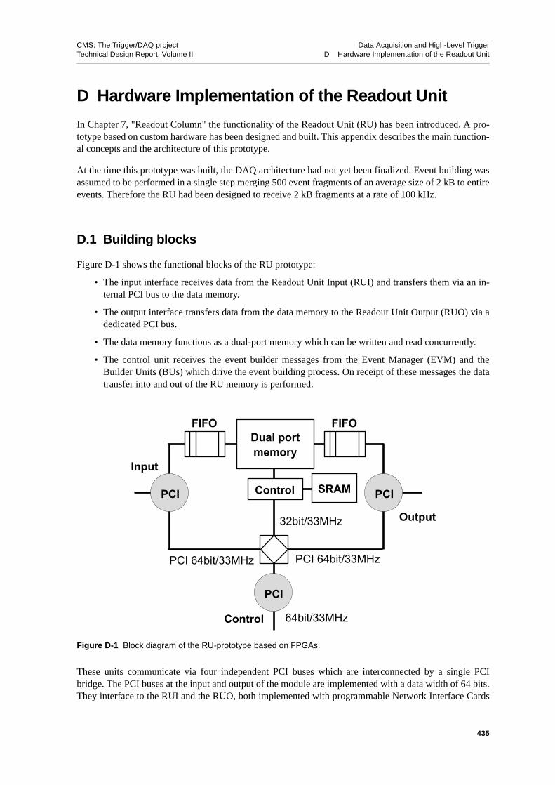
CMS: The Trigger/DAQ project Data Acquisition and High-Level TriggerTechnical Design Report, Volume II D Hardware Implementation of the Readout Unit
D Hardware Implementation of the Readout Unit
In Chapter 7, "Readout Column" the functionality of the Readout Unit (RU) has been introduced. A pro-totype based on custom hardware has been designed and built. This appendix describes the main function-al concepts and the architecture of this prototype.
At the time this prototype was built, the DAQ architecture had not yet been finalized. Event building wasassumed to be performed in a single step merging 500 event fragments of an average size of 2 kB to entireevents. Therefore the RU had been designed to receive 2 kB fragments at a rate of 100 kHz.
D.1 Building blocks
Figure D-1 shows the functional blocks of the RU prototype:
• The input interface receives data from the Readout Unit Input (RUI) and transfers them via an in-ternal PCI bus to the data memory.
• The output interface transfers data from the data memory to the Readout Unit Output (RUO) via adedicated PCI bus.
• The data memory functions as a dual-port memory which can be written and read concurrently.
• The control unit receives the event builder messages from the Event Manager (EVM) and theBuilder Units (BUs) which drive the event building process. On receipt of these messages the datatransfer into and out of the RU memory is performed.
These units communicate via four independent PCI buses which are interconnected by a single PCIbridge. The PCI buses at the input and output of the module are implemented with a data width of 64 bits.They interface to the RUI and the RUO, both implemented with programmable Network Interface Cards
Figure D-1 Block diagram of the RU-prototype based on FPGAs.
Dual portmemory
Control
Control
FIFO FIFO
SRAM
Input
Output
PCI 64bit/33MHzPCI 64bit/33MHz
64bit/33MHz
32bit/33MHz
PCI PCI
PCI
435

CMS: The Trigger/DAQ project Data Acquisition and High-Level TriggerTechnical Design Report, Volume II D Hardware Implementation of the Readout Unit
(NICs). The control bus and the internal PCI bus are 32 bits wide. All buses are clocked at 33 MHz. Thecontrol messages for event building in principle can be received via any of the three PCI interfaces, sinceall PCI buses are interconnected by a bridge. In the tests performed, the messages from the EVM havebeen received via the interface to the host PC whereas the Builder Unit requests were issued by the RUO.
D.2 RU Memory Design
The memory of the RU is the main data buffer in the Readout Column. It is required to buffer the datastream of at least one second of data taking at full level 1 trigger rate. With a mean event fragment size of2 kB this means a buffer memory of at least 200 MB. The RU implements its main buffer with a cost ef-fective DIMM II memory module which is available on the PC market. Modules with up to 512 MB canbe used. Since the memory is accessed simultaneously from the input and the output of the RU, some ar-bitration logic is needed to control the data traffic.
D.2.1 Data Input and Data Output Stream
At 100 kHz trigger rate and an average event fragment size of 2 kB the data throughput of the RU is200 MB/s. Event fragments are stored in the buffer memory until they are requested by a BU. The incom-ing and the outgoing data streams are asynchronous to each other. Therefore the data memory is designedas a dual ported memory which can be written an read simultaneously. The memory bus operates at a fre-quency of 66 MHz with a data width of 64 bits. The resulting memory bandwidth of 528 MB/s is sharedbetween the input stage and the output stage. The control logic of the memory ensures that the memorycan be written and read with 200 MB/s concurrently.
D.2.2 Memory Organization
The order in which the BUs request event fragments from the RU is in general different from the order inwhich fragments are stored in the RU. Since in addition the fragments have a variable length, a MemoryManagement Unit (MMU) has been developed. The entire memory space is divided into fixed size blocks(the size of the blocks is programmable). Pointers to available memory blocks are held in a list imple-mented as a FIFO. Incoming data is written into as many data blocks as needed to hold the entire frag-ment. The information on how the blocks are chained is held in a separate RAM table. Once the fragmenthas been transferred to the output, the corresponding memory blocks are made available to newly incom-ing data by writing their pointers back into the list.
D.3 Event Fragment Control Logic
Incoming event fragments are associated with an unique event identifier received from the event manager.The same event identifier is used by the BU to request a specific event fragment. This means that the RUmust be able to find the chain of memory blocks associated to a specific event identifier, in order to trans-fer the corresponding data to the RUO. For this purpose a look-up table is implemented in the RU. It isaddressed with the event identifier and contains data fragment descriptors which contain information rel-evant for the efficient data transfer to the RUO.
436

CMS: The Trigger/DAQ project Data Acquisition and High-Level TriggerTechnical Design Report, Volume II E Fault Tolerance of Distributed Systems
E Fault Tolerance of Distributed Systems
The main issue is how to demonstrate the fault tolerance properties of a distributed system. There are twomethods that have been used in the field of computer science:
• formal correctness proofs
• fault injection
Although formal methods provide valuable tools for identifying errors in some contexts, these tools lackthe sensitivity, for example, to detect timing problems which are crucial for the DAQ system. Hence thesemethods are not considered in this document.
Before discussing the fault-injection procedure, the overall program is defined:
1. The current DAQ system design is supplemented in places that have been identified as potentialsources of faults with additional functionality or improved components.
2. The design is established to be fault-tolerant after the current design is supplemented with the ele-ments in the previous step. To do this, it is demonstrated that the current system and its associatedprotocols are such that all transient faults are handled in real-time and that, after relatively short pe-riods of time, the system resumes its correct operation.
3. The implementation of the established fault-tolerant protocols is tested by using prototype softwareand hardware developed in the context of the CMS-DAQ R&D. This the step where fault-injectiontests are carried out
Step-3, which is usually not included in error analyses of DAQ systems, is particularly important becausefault-handling code is exercised only when a fault occurs. Given that the occurrence of faults should bethe exception, rather than the rule, such code is therefore either not tested, or is only minimally tested. Toestablish the correctness and scaling of the fault handling mechanisms in the design, fault injection at thelevel of the prototype Event Builder and in a simulation of the full CMS system is used to establish thecorrectness of the actual implementation.
E.1 Failure Modes of Distributed Systems
In order to define the possible failure modes of distributed systems, the general properties of a distributedsystem must be defined.
A distributed system is a collection of nodes, where a node is any device or software package which has aself-contained function. For example, an Event Manager process running in a computer is a node; similar-ly for Readout Units or Builder Units. Another type of node particular to CMS is the Front-end ReadoutLink hardware module. In general, a node provides a service. A service-provider executes a collection ofoperations which can be self-triggered by passage of time or can be triggered by client-requests. Our Da-ta-Acquisition system is therefore a collection of nodes or service-providers which interact with one an-other. An example is when an Event-Manager provides to a Builder-Unit an identification of the nextevent waiting to be assembled upon request from it. In return, the Builder-Unit notifies the event managerof the completion of the event assembly.
A server may implement its service by using the services of other servers. For example, the Event-Man-ager application, in providing a service to the Builder-Unit, can use a "Datagram" service which sendsmessages as sequences of packets; the Datagram server might in turn depend on the physical communica-
437

CMS: The Trigger/DAQ project Data Acquisition and High-Level TriggerTechnical Design Report, Volume II E Fault Tolerance of Distributed Systems
tion server which is used. Thus, the user/client and resource/server names are relative to the “depends” re-lation: what is a resource or server at a certain level of abstraction can be a client or a user at another levelof abstraction [E-1].
A server performs a correct service if it behaves in a manner consistent with its service specification; thatis, its outputs of internal state-transitions are correct. A failure occurs when the delivered service no long-er complies with the agreed description of the system’s expected service [E-2]. Failure is a property of theexternal behaviour of a service-providing system — which is itself a manifestation of its internal statesand state transitions [E-3]. A service may not, and generally does not, always fail in the same way. Theways a service can fail are its failure modes.
In a distributed system, a node is an appropriate unit of failure. The node implementation maps internalnode failures into simple external failure modes [E-4]. Faults which affect only the internal state of anode, but do not propagate to the rest of the system can not affect the correctness of the behaviour (or in-tegrity) of the entire system [E-5]. The failure modes of nodes are thus defined in terms of the messagesthat faulty nodes send or do not send. Such nodes can fail, according to the service specification domainsdescribed above, by producing messages with erroneous content, messages that arrive untimely, or indeed“impromptu” messages that should never have been sent at all [E-6].
E.1.1 Fault Model Hierarchy
A subset of possible transaction faults in a computing system which is relevant to CMS-DAQ is shown inFigure E-1.Incorrect timing with a correct result is called a timing fault. In a timing fault, the correct re-sult is delivered from a component either too early, too late or never. Timing faults can affect either acomputational process or an inter-node message. Timing faults in processes that do not affect the associat-
Figure E-1 Possible transaction faults in a computing system relevant to CMS-DAQ system. A detailed analysiscan be found in references [E-1] and [E-2].
Incorrect Computation
Timing Message Corruption
Spurious Messages
Replication Generation
Accelerated Delay Omission
Incorrect Timing but Correct Result
Incorrect Result
Internode Message
Early Late Never
438

CMS: The Trigger/DAQ project Data Acquisition and High-Level TriggerTechnical Design Report, Volume II E Fault Tolerance of Distributed Systems
ed node’s output are not considered. Process timing that do affect output lead to one of the other faulttypes shown in Figure E-1.
• accelerated fault: a message is delivered before it is expected.
• delay faults message arrives at a destination later than expected.
• omission fault: a message never arrives. An omission fault can occur at the node level and can beeither a send or a receive omission, or it can occur at the link level.
• link omission fault: occurs when a communication link drops one or more messages.
• receive omission: occurs when a node fails to receive a required message and behaves asthough it did not arrive.
• send omission occurs when a node fails to send a required message. Send omissions are par-ticularly important since they can be used to emulate fail-silent1, crash2, and fail-stop3
faults. From the communication standpoint, all three of these fault types can be emulated bysend omission on all messages.
An incorrect result produced at a correct time can also be seen by a client as a timing fault. This can hap-pen when the time at which a message is sent depends on a computed result. In fact, depending on how itis used, an incorrect result can lead to almost any type of fault. Two other types of such faults are messagecorruption and spurious messages.
In message corruption, the contents of a message are changed. Either field of a message, header or data,can be corrupted. The resulting error behaviour of the receiver depends on the which field within theheader gets corrupted. Since message corruption can occur prior to a message being encoded for transmis-sion, coding techniques are not sufficient to handle this type of fault.
A spurious message occurs when a node receives a message that it is not expecting. Spurious messagescan occur in a variety of situations. For example, some failure modes may result in message replication,i.e. multiple copies of a message being sent. Other failure modes may cause message generation, where amessage is produced when it should not be. A message which is sent to the wrong destination causes aspurious message at the new destination and an omission at the intended destination.
Faults occurring in the Event Builder can be analyzed at two abstraction levels: a system level and a spe-cific component level. System-level faults are those faults that are independent of the specifics of the im-plementation of the system-components. On the other hand, specific-element faults depend on the detailsof the implementation. By using an abstraction at the system or functional level, faults specific to thefunctionality of the system can be analyzed. The relation of system-level faults to specific-element faultsis a many-to-many association. Each system-level fault originates from one or more lower-level faults. Asan illustration, consider the case of a bit-flip failure in a packet header. As a result of such a bit-flip fault,the possible system-level failure is a miss-routed message, which results in an omission failure and a spu-rious message. Note that the final observable, the omission failure of the current example, may arise be-cause of numerous faults, for example, from a buffer overflow in a receiver Network-Interface-Card.
The system-level abstraction has the advantage of analysing the system without a reference to a particularimplementation. As long as the faults belonging to the lower level and the system-level abstractions havethe same coverage, in the following analysis it will be sufficient to consider only the system level faults.
1.A fail-silent node stops producing messages although its internal state may continue to be updated.2.In a crash fault, the node stops sending messages and the internal state may be lost completely.3.A fail-stop node halts but maintains the internal state it had just prior to halting.
439

CMS: The Trigger/DAQ project Data Acquisition and High-Level TriggerTechnical Design Report, Volume II E Fault Tolerance of Distributed Systems
A transient fault [E-4] is a class of faults which exist only for a short interval of time and disappear with-out an explicit repair action from a higher authority. A transient fault might lead the system into an errorstate which can be permanent. If this error state is not detected and handled properly, it will lead to a sys-tem failure which will degrade the system availability and reliability. A system with the ability to recoverfrom inconsistent states caused by transient faults without an outside intervention and regardless of thefault’s origin, is said to be a self-stabilizing system [E-2].
The DAQ system will automatically recover to a consistent state if all sub-systems recover within a finitetime interval from inconsistent states. This self-stabilizing property of the event-building part of the DAQsystem can be guaranteed even in the case of transient faults. However, the self-stabilizing property doesnot necessarily guarantee a continuous reliability.
E.2 Fault Classification
In a distributed system, faults occurring in a subsystem can affect overall system behaviour only if theypropagate into other subsystems. Inversely, faults which affect only the internal state of a subsystem, butdo not propagate to the rest of the system, cannot affect the correctness of the behaviour of the entire sys-tem. This property allows the emulation of each possible failure by a corresponding transaction failure[E-6]. Another consequence of this property is that the origin of a fault cannot be identified uniquely.
An in-depth study of this classification of transaction faults has been done in [E-1]. A specific implemen-tation in the domain of performance evaluation using fault-injection techniques is described in [E-6]. Theanalysis can be significantly simplified, if only the possible observable transaction failures relevant toCMS are considered, as shown in Figure E-1.
In the classification of Figure E-1 there are three main classes of faults: those relating to timing, messagecorruption and spurious messages. In order to prove that the design is fault-tolerant, it must be shown thatthere are three and only three fault classes and that there exist such protocol extensions that are can detectand recover from these faults. The first part of the proof is not tractable formally, and therefore complete-ness cannot be claimed. Instead the analysis proceeds with a description of all possible faults that can beidentified.
E.3 References
E-1 C. Flaviu, “Understanding Fault-Tolerant Distributed Systems”, CACM, February 1991.
E-2 J. C. Laprie, “Dependability: Basic Concepts and Terminology”, IFIP WG 10.4 Dependable Computing and Fault Tolerance. Springer,1992
E-3 J. Rushby, “Critical System Properties: Survey and Taxonomy”, Reliability Engineering and System Safety, 43 (1194) 189.
E-4 H. Kopetz, “Real-Time Systems: Design Principles for Distributed Embedded Applications”, Kluwer Academic Publishers, 1997.
E-5 D. M. Blough and T. Torii, “Fault-Injection-Based Testing of Fault-Tolerant Algorithms”, in Message-Passing Parallel Computers, IEEE 27th Annual International Symposium on Fault Tolerant Computing, 1997.
E-6 C. Flaviu, “Abstraction for Fault-Tolerance”, 13th IFIP World Computer Congress, Hamburg, 1994.
440

CMS: The Trigger/DAQ project Data Acquisition and High-Level TriggerTechnical Design Report, Volume II F Summary of Level-1 Trigger
F Summary of Level-1 Trigger
The Level-1 Trigger System [F-1] is organized into three major subsystems: the Level-1 calorimeter trig-ger, the Level-1 muon trigger, and the Level-1 global trigger. The muon trigger is further organized intosubsystems representing the 3 different muon detector systems, the Drift Tube Trigger in the barrel, theCathode Strip Chamber (CSC) trigger in the endcap and the Resistive Plate Chamber (RPC) trigger cov-ering both barrel and endcap. The Level-1 muon trigger also has a global muon trigger that combines thetrigger information from the DT, CSC and RPC trigger systems and sends this to the Level-1 global trig-ger. A diagram of the Level-1 Trigger system is shown in Figure F-1.
The data used as input to the Level-1 Trigger system as well as the input data to the global muon trigger,global calorimeter trigger and the global trigger are transmitted to the DAQ for storage along with theevent readout data. In addition, all trigger objects found, whether they were responsible for the Level-1Trigger or not, are also sent. The decision whether to trigger on a specific crossing or to reject that cross-ing is transmitted via the Trigger Timing and Control system to all of the detector subsystem front-endand readout systems.
F.1 Calorimeter Trigger Description
The calorimeter trigger begins with (0.35η×0.35φ) trigger tower energy sums formed by the ECAL,HCAL and HF upper level readout Trigger Primitive Generator (TPG) circuits from the individual calo-rimeter cell energies. For the ECAL, these energies are accompanied by a bit indicating the transverse ex-tent of the electromagnetic energy deposit. For the HCAL, the energies are accompanied by a bitindicating the presence of minimum ionizing energy. The TPG information is transmitted over high speedcopper links to the Regional Calorimeter Trigger (RCT), which finds candidate electrons, photons, taus,and jets. The RCT separately finds both isolated and non-isolated electron/photon candidates. The RCTtransmits the candidates along with sums of transverse energy to the Global Calorimeter Trigger (GCT).
Figure F-1 Overview of the Level-1 Trigger system.
HFenergy
HCALenergy
ECALenergy
RPChits
DThits
CSChits
RegionalCal. Trigger
GlobalCal. Trigger
PatternComp-arator
segmentfinder
segmentfinder
track finder
track finder
Global Muon Trig ger
Global Trigger TTC System TRK,ECAL,HCAL,MU
quietregions
& mip bits
DAQ
triggerprimitivedata
inputdata
triggerobjects
441
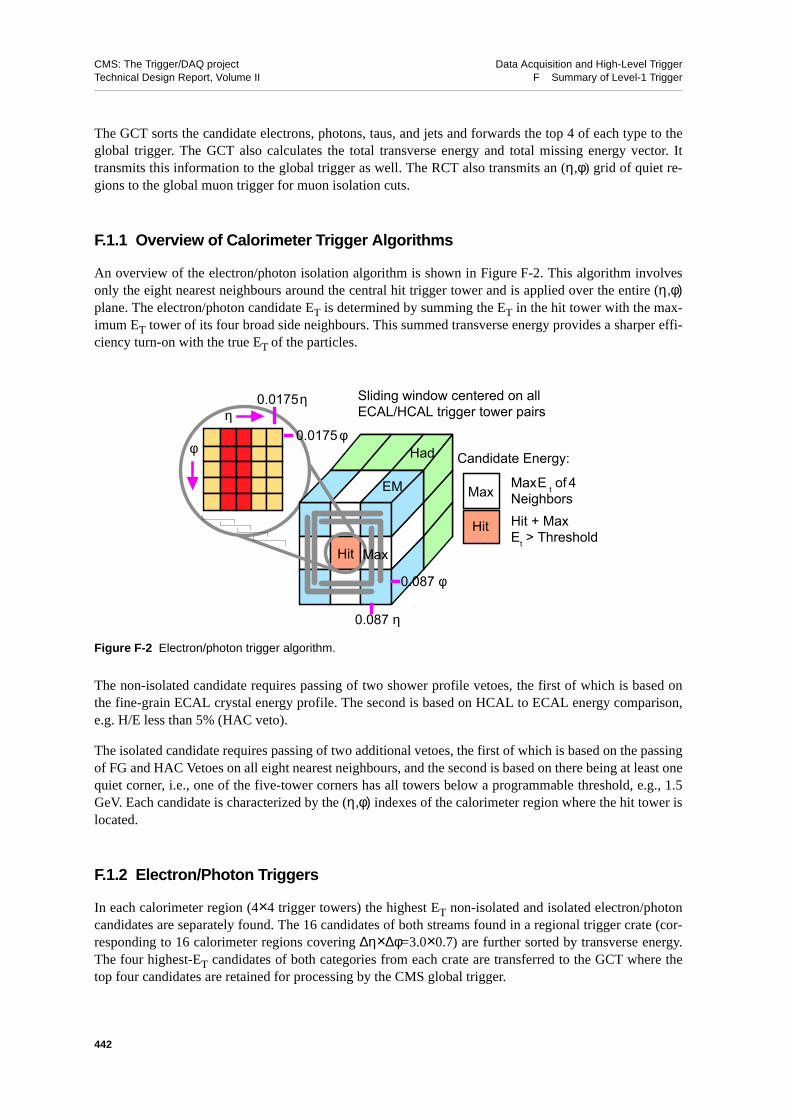
CMS: The Trigger/DAQ project Data Acquisition and High-Level TriggerTechnical Design Report, Volume II F Summary of Level-1 Trigger
The GCT sorts the candidate electrons, photons, taus, and jets and forwards the top 4 of each type to theglobal trigger. The GCT also calculates the total transverse energy and total missing energy vector. Ittransmits this information to the global trigger as well. The RCT also transmits an (η,φ) grid of quiet re-gions to the global muon trigger for muon isolation cuts.
F.1.1 Overview of Calorimeter Trigger Algorithms
An overview of the electron/photon isolation algorithm is shown in Figure F-2. This algorithm involvesonly the eight nearest neighbours around the central hit trigger tower and is applied over the entire (η,φ)plane. The electron/photon candidate ET is determined by summing the ET in the hit tower with the max-imum ET tower of its four broad side neighbours. This summed transverse energy provides a sharper effi-ciency turn-on with the true ET of the particles.
The non-isolated candidate requires passing of two shower profile vetoes, the first of which is based onthe fine-grain ECAL crystal energy profile. The second is based on HCAL to ECAL energy comparison,e.g. H/E less than 5% (HAC veto).
The isolated candidate requires passing of two additional vetoes, the first of which is based on the passingof FG and HAC Vetoes on all eight nearest neighbours, and the second is based on there being at least onequiet corner, i.e., one of the five-tower corners has all towers below a programmable threshold, e.g., 1.5GeV. Each candidate is characterized by the (η,φ) indexes of the calorimeter region where the hit tower islocated.
F.1.2 Electron/Photon Triggers
In each calorimeter region (4×4 trigger towers) the highest ET non-isolated and isolated electron/photoncandidates are separately found. The 16 candidates of both streams found in a regional trigger crate (cor-responding to 16 calorimeter regions covering ∆η×∆φ=3.0×0.7) are further sorted by transverse energy.The four highest-ET candidates of both categories from each crate are transferred to the GCT where thetop four candidates are retained for processing by the CMS global trigger.
Figure F-2 Electron/photon trigger algorithm.
Sliding window centered on allECAL/HCAL trigger tower pairs
Max E t of 4NeighborsHit + MaxEt > Threshold
Hit
Max
Candidate Energy:
0.0175 η
φ
η
Hit
0.087 η
0.087 φ
Max
0.0175 φHad
EM
442

CMS: The Trigger/DAQ project Data Acquisition and High-Level TriggerTechnical Design Report, Volume II F Summary of Level-1 Trigger
The nominal electron/photon algorithm allows both non-isolated and isolated streams. The non-isolatedstream uses only the hit tower information except for adding in any leakage energy from the maximumneighbour tower. This stream will be used at low luminosity to provide the B-electron trigger. The isola-tion and shower shape trigger cuts are programmable and can be adjusted to the running conditions. Forexample, at high luminosity the isolation cuts could be relaxed to take into account higher pile-up ener-gies. The specification of the electron/photon triggers also includes the definition of the η−φ region whereit is applicable. In particular, it is possible to define different trigger conditions (energy thresholds, isola-tion cuts) in different rapidity regions.
The efficiency of the electron/photon algorithm, as a function of the electron transverse momentum, fordifferent thresholds applied at Level-1, is shown in Figure F-3. Also shown in Figure F-3 is the efficiency,as function of pseudorapidity for electrons with PT=35 GeV/c.
To connect the Level-1 threshold to an effective requirement on the electron transvsers momentum, theelectron PT at which the Level-1 Trigger is 95% efficient, is determined as function of the Level-1 thresh-old. This is shown in Figure F-4.
Figure F-3 The efficiency of the Level-1 Trigger for single electrons as a function of the electron PT. On theright, the efficiency, as function of η, for electrons with PT=35 GeV/c.
Figure F-4 The electron ET at which the Level-1 Trigger is 95% efficient as a function of the Level-1 threshold.
0
0.2
0.4
0.6
0.8
1
0 5 10 15 20 25 30 35 40 45 50
1034
14 18 22 26 30
16 20 24 28
Electron Pt [GeV]
95% 90%
Effic
ienc
y
0.6
0.7
0.8
0.9
1
-2 -1 0 1 2
Effic
ienc
y
η
0
5
10
15
20
25
30
35
40
45
50
0 5 10 15 20 25 30 35 40 45 50
Level-1 threshold [GeV]
T90 = 4.12 + 0.981 * TL-1
T95 = 5.34 + 1.010 * TL-1
Elec
tron
Pt [
GeV
]
443

CMS: The Trigger/DAQ project Data Acquisition and High-Level TriggerTechnical Design Report, Volume II F Summary of Level-1 Trigger
From this result, the rate for electron/photon triggers as a function of the effective cut on the ET, i.e. of thepoint at which the trigger is 95% efficient, can be computed. Figure F-5 shows the rates for single elec-trons as a function of the ET of the electron (95% point).
Double, triple and quad electron/photon triggers can be defined. The requirements on the objects of amulti electron/photon trigger, namely the energy threshold, the cluster shape and isolation cuts and the(η,φ) region, are set individually. Requirements on the (η,φ) separation between objects can also be de-fined. The rate for two-electron/photon triggers is shown in Figure F-6.
Figure F-5 The rate of the single electron/photon Level-1 Trigger at low (left) and high (right) luminosity.
Figure F-6 The rate of the double electron/photon Level-1 Trigger at low (left) and high (right) luminosity.
1
10
10 2
10 3
20 25 30 35 40 451
10
10 2
10 3
20 25 30 35 40 45
Level-1 ET (95%) [GeV]
Rat
e [k
Hz]
Level-1 single e.m.1034/cm2/s
AllAfter FG + HoEAfter isolation
10-1
1
10
2
20 25 30 35 40 4510
-1
1
10
10 2
20 25 30 35 40 45
Level-1 ET (95%) [GeV]
Rat
e [k
Hz]
Level-1 single e.m.2x1033/cm2/s
AllAfter FG + HoEAfter isolation
10-1
1
10
10 2
10 15 20 2510
-1
1
10
10 2
10 15 20 25
Level-1 ET(95%) [GeV]
Rat
e [k
Hz]
Level-1 double e.m.2x1033/cm2/s
AllAfter FG + HoEAfter isolation
10-1
1
10
10 2
10 15 20 2510
-1
1
10
10 2
10 15 20 25
Level-1 ET(95%) [GeV]
Rat
e [k
Hz]
Level-1 double e.m.1034/cm2/s
AllAfter FG + HoEAfter isolation
444

CMS: The Trigger/DAQ project Data Acquisition and High-Level TriggerTechnical Design Report, Volume II F Summary of Level-1 Trigger
F.1.3 Jet and τ Triggers
The jet trigger uses the transverse energy sums (em+had) computed in calorimeter regions (4×4 triggertowers), except in the HF region where it is the trigger tower itself. The input tower ET is coded in an 8 bitlinear scale with programmable resolution. Values exceeding the dynamic range are set to the maximum.The subsequent summation tree extends to a 10 bit linear scale with overflow detection. Simulation stud-ies showed that a scale of 10 bits with LSB=1 GeV gives adequate jet trigger performance.
The jet trigger uses a 3×3 calorimeter region sliding window technique which spans the complete (η,φ)coverage of the CMS calorimeters (Figure F-7) seamlessly. The central region ET is required to be higherthan the eight neighbour region ET values. In addition, the central region ET is required to be greater thana fixed value, e.g., 5 GeV, to suppress spurious soft.
The jets and τs are characterized by the transverse energy ET in 3×3 calorimeter regions. The summationspans 12×12 trigger towers in barrel and endcap or 3×3 larger HF towers in the HF. The φ size of the jetwindow is the same everywhere. The η binning gets somewhat larger at high η due to the size of calorim-eter and trigger tower segmentation. The jets are labelled by (η,φ) indexes of the central calorimeter re-gion.
Single and three-prong decays of τ leptons form narrow clusters of energy deposits in the calorimeter.Since the decays involve charged pions which deposit energies in the hadron calorimeter, the elec-tron/photon trigger does not capture them. Therefore, the transverse profiles of active tower patterns areanalysed to tag narrow jets as potential τ lepton decays. An active tower is defined as a trigger tower withECAL or HCAL ET above a separately programmable threshold. The calorimeter region has τ-veto setON if the active towers do not form any of the 8 patterns shown in the Figure F-7, i. e., the pattern is notconfined within 2×2 contiguous trigger towers of the calorimeter region. A jet is defined as “τ-like” ifnone of the 9 calorimeter region τ-veto bits are ON. The τ-veto bits are therefore used for both τ-like en-ergy deposit identification and quite stringent isolation. This strict isolation requirement is tolerable be-cause such cuts are necessary to find τs even in later offline analysis.
In addition counters of the number of jets above programmable thresholds in various η regions are pro-vided to give the possibility of triggering on events with a large number of low energy jets. Jets in the for-
Figure F-7 Jet and τ trigger algorithms.
TriggerTower
E CAL
HCAL
= 0.348PbWO4 Crystal
= 1.04
445

CMS: The Trigger/DAQ project Data Acquisition and High-Level TriggerTechnical Design Report, Volume II F Summary of Level-1 Trigger
ward and backward HF calorimeters are sorted and counted separately. This separation is a safetymeasure to prevent more background susceptible high η region from masking central jets. Although thecentral and forward jets are sorted and tracked separately through the trigger system, the global triggercan use them seamlessly as the same algorithm and resolutions are used for the entire η−φ plane.
Single, double, triple and quad jet (τ) triggers are possible. The single jet (τ) trigger is defined by thetransverse energy threshold, the (η,φ) region of validity and eventually by a prescaling factor. Prescalingwill be used for low energy jet (τ) triggers, necessary for efficiency measurements. The multi jet (τ) trig-gers are defined by the number of jets (τs) and their transverse energy thresholds, by a minimum separa-tion in (η,φ), as well as by a prescaling factor. The global trigger accepts the definition, in parallel, ofdifferent multi jet (τ) triggers conditions.
The four highest energy central and forward jets, and central τs in the calorimeter are selected. Jets and τsoccurring in a calorimeter region where an electron is identified are not considered. The selection of thefour highest energy central and forward jets and of the four highest energy τs provides enough flexibilityfor the definition of combined triggers.
Figure F-8 shows the Level-1 rates for jet triggers at low and high luminosity. Another quantity of inter-est, which is also useful in making comparisons between different algorithms and different detectors, isthe rate as a function of the generator-level jet ET by plotting the rate for the cut on offline jet ET thatgives 95% efficiency for the generator-level jet ET. This is shown in Figure F-9
F.1.4 Energy Triggers
The ET triggers use the transverse energy sums (em+had) computed in calorimeter regions (4×4 triggertowers in barrel and endcap). Ex and Ey are computed from ET using the coordinates of the calorimeter re-gion center. The computation of missing transverse energy from the energy in calorimeter regions doesnot affect significantly the resolution for trigger purposes.
The missing ET is computed from the sums of the calorimeter regions Ex and Ey. The sum extends up tothe end of forward hadronic calorimeter, i.e., |η|=5. The missing ET triggers are defined by a threshold
Figure F-9 Rate for the cut on Level-1 jet ET that is 95% efficient for jets with generator-level ET of the valuegiven on the x-axis versus generator-level ET. Left: low luminosity; right: high luminosity.
L = 2x1033cm-2s-1
L1 jets
Single JetDouble JetTriple JetQuad Jet
Particle Jet Et, 95% Eff [GeV]
Rat
e [H
z]
10-2
10-1
1
10
10 2
10 3
10 4
10 5
10 6
10 7
0 200 400 600 800 1000
L = 1034cm-2s-1
L1 JetsSingle JetDouble JetTriple JetQuad Jet
Particle Jet Et, 95% Eff [GeV]
Rat
e [H
z]
10-2
10-1
1
10
10 2
10 3
10 4
10 5
10 6
10 7
0 200 400 600 800 1000
446

CMS: The Trigger/DAQ project Data Acquisition and High-Level TriggerTechnical Design Report, Volume II F Summary of Level-1 Trigger
value and by a prescaling factor. The global trigger accepts the definition, in parallel, of different missingET triggers conditions.
The total ET is given by the sum of the calorimeter regions ET. The sum extends up to the end of forwardcalorimeter, i.e., |η|=5. The total ET triggers are defined by a threshold value and by a prescaling factor.The global trigger accepts the definition, in parallel, of different total ET triggers conditions. The total en-ergy trigger is implemented with a number of thresholds which are used both for trigger studies and forinput to the luminosity monitor. Some of these thresholds are used in combination with other triggers.Other thresholds are used with a prescale and one threshold is used for a stand-alone trigger. The lowerthreshold ET trigger also provides a good diagnostic for the calorimeter and its trigger.
The HT trigger is defined as the scalar sum of the ET of jets above a programmable threshold with a typi-cal value of jet ET > 10 GeV. This trigger is not as susceptible as the total ET given by the sum of the cal-orimeter regions ET deposits to both noise and pileup effects. The Although total ET is a necessarytechnical trigger, it has limited use from physics point of view. The HT trigger can capture high jet multi-plicity events such as those from fully hadronic top decay, hadronic decays of squarks and gluinos. Al-though these events have several hundred GeV/c2 energy, they may actually fail the jet triggers becauseindividual jet ETs may be quite a bit softer than the sustainable thresholds. In addition, the HT trigger canuse individually calibrated jet energies unlike the total ET trigger which cannot be easily calibrated.
F.2 Muon Trigger Description
Each of the Level-1 muon trigger systems has its own trigger logic. The RPC strips are connected to aPattern Comparator Trigger (PACT), which is projective in η and φ. The PACT forms trigger segmentswhich are connected to segment processors which find the tracks and calculate the PT. The RPC logic alsoprovides some hit data to the CSC trigger system to improve resolution of ambiguities caused by 2 muonsin the same CSC.
The Cathode Strip Chambers form Local Charged Tracks (LCT) from the Cathode Strips, which are com-bined with the Anode wire information for bunch crossing identification on a Trigger Motherboard TheLCT pattern logic assigns a PT and quality, which is used to sort the LCT on the Motherboard and the
Figure F-8 Level-1 jet trigger rates for low and high luminosity.
L = 1034
cm-2s
-1
L1 JetsSingle JetDouble JetTriple JetQuad Jet
Calibrated Et Cutoff [GeV]
Rat
e [H
z]
10-2
10-1
1
10
10 2
10 3
10 4
10 5
10 6
10 7
0 200 400 600 800 1000
L = 1034
cm-2s-1
L1 JetsSingle JetDouble JetTriple JetQuad Jet
Calibrated Et Cutoff [GeV]R
ate
[Hz]
10-2
10-1
1
10
10 2
10 3
10 4
10 5
10 6
10 7
0 200 400 600 800 1000
447
CMS: The Trigger/DAQ project Data Acquisition and High-Level TriggerTechnical Design Report, Volume II F Summary of Level-1 Trigger
Muon Port Card that collects LCTs from up to 9 CSC chambers. The top 3 LCTs from all the MPCs in asector are transmitted to the CSC Track Finder, which combines the LCTs into full muon tracks and as-signs PT values to them. The CSC and Drift Tube Track-Finders exchange track segment information inthe region where the chambers overlap.
The Barrel Muon Drift Tubes are equipped with Bunch and Track Identifier (BTI) electronics that findstrack segments from coincidences of aligned hits in 4 layers of one drift tube superlayer. The track seg-ments positions and angles are sent to the Track Correlator (TRACO), which attempts to combine the seg-ments from the two Super Layers (SL) measuring the φ coordinate. The best combinations from allTRACOs of a single chamber together with the SL η segments are collected by the Trigger Server. TheTrigger Server then sends the best two segments (if found) to the Track Finder, which combines the seg-ments from different stations into full muon tracks and assigns PT values to them.
The Global Muon Trigger sorts the RPC, DT and CSC muon tracks, converts these tracks into the same η,φ and PT scale, and validates the muon sign. It then attempts to correlate the CSC and DT tracks with RPCtracks. It also correlates the found muon tracks with an η-φ grid of quiet calorimeter towers to determineif these muons are isolated. The final ensemble of muons are sorted based on their initial quality, correla-tion and pT and then the 4 top muons are sent to the Global Trigger.
F.2.1 Overview of Muon Trigger Algorithms
The logical structure of the Muon Trigger is shown in Figure F-10. DT and CSC electronics first processthe information from each chamber locally. Therefore they are called local triggers. As a result one vector(position and angle) per muon per station is delivered. Vectors from different stations are collected by theTrack Finder (TF) which combines them to form a muon track and assigns a transverse momentum value.TF plays the role of a regional trigger. Up to 4 best (highest PT and quality) muon candidates from eachsystem are selected and sent to the Global Muon Trigger.
In the case of RPC there is no local processing apart from synchronisation and cluster reduction. Hitsfrom all stations are collected by PACT logic. If they are aligned along a possible muon track, a pT valueis assigned and the information is sent to the Muon Sorter. The Muon Sorter selects 4 highest pT muonsfrom the barrel and 4 from the endcaps and sends them to the Global Muon Trigger. The Global MuonTrigger compares the information from TF (DT/CSC) and PACT (RPC). Quiet bits delivered by the Calo-rimeter Trigger are used to form an isolated muon trigger. The 4 highest pT muons in the whole event arethen transmitted to the Global Trigger. Finally transverse momentum thresholds are applied by the GlobalTrigger for all trigger conditions.
F.2.2 Drift Tube Trigger
The drift chambers deliver data for track reconstruction and triggering on different data paths. The localtrigger is based on two SL in the φ view of the muon station. The trigger front-end, called the Bunch andTrack Identifier (BTI), is used in the φ view and the θ view to perform a rough muon track fit in one sta-tion measuring position and direction of trigger candidate tracks with at least three hits, in different planesof a Super Layer (SL). The algorithm fits a straight line within programmable angular acceptance. TheBTI performs the bunch crossing assignment of every found muon track candidate. The algorithm used inthe device is a generalization of the mean-timer method [F-2].
Since this method must foresee alignment tolerances and needs to accept alignments of only three hits, thealgorithm can generate false triggers. Hence in the bending plane a system composed by a Track Correla-
448

CMS: The Trigger/DAQ project Data Acquisition and High-Level TriggerTechnical Design Report, Volume II F Summary of Level-1 Trigger
tor (TRACO) and a chamber Trigger Server (TS) is used to filter the information of the two φ SLs of achamber in order to lower the trigger noise. The TRACO/TS block selects, at every cycle among the trig-ger candidates, at most two tracks with the smallest angular distances (i.e. higher PT) with respect to theradial direction to the vertex.
Track segments found in each station are then transmitted to a regional trigger system called Drift TubeTrack Finder (DTTF). The task of the Track Finder is to connect track segments delivered by the stationsinto a full track and assign a transverse momentum value to the finally resolved muon track. The systemis divided in sectors, each of them covering 30° in the φ angle. Each Sector Processor is logically dividedin three functional units - the Extrapolator Unit (EU), the Track Assembler (TA) and the AssignmentUnits (AU), as shown in Figure F-11.
The Extrapolator Unit attempts to match track segments pairs of distinct stations. Using the spatial coor-dinate φ and the bending angle of the source segment, an extrapolated hit coordinate is calculated. Thetwo best extrapolations per each source are forwarded to the Track Assembler. The Track Assembler at-tempts to find at most two tracks in a detector sector with the highest rank, i.e. exhibiting the highestnumber of matching track segments and the highest extrapolation quality.Once the track segment data areavailable to the Assignment Unit, memory based look up tables are used to determine the transverse mo-mentum, the φ and η coordinates, and a track quality.
Figure F-10 Block diagram of the Level-1 muon trigger.
Quiet Bits from Calo Trigger
To Global Trigger
Global Muon Trigger
CSCEndcap
Wirecards
Stripcards
Motherboard
Port card
CSCCathode Strip Ch.
Track Finder
DTTFDrift Tube
Track Finder
TriggerServer
TRACOTrack Correlator
BTIBunch & Time IO
CSCSorter
DT Sorter
DTBXBarrel
RPCSorter
PACTPattern
Comparator
RPC
449

CMS: The Trigger/DAQ project Data Acquisition and High-Level TriggerTechnical Design Report, Volume II F Summary of Level-1 Trigger
F.2.3 CSC Trigger
The task of the Cathode Strip Chamber (CSC) Track-Finder is to reconstruct tracks in the CSC endcapmuon system and to measure the transverse momentum (PT), pseudo-rapidity (η), and azimuthal angle (φ)of each muon. The measurement of PT by the CSC trigger uses spatial information from up to three sta-tions to achieve a precision similar to that of the DT Track-Finder despite the reduced magnetic bendingin the endcap. The CSC Local Trigger provides high rejection power against these backgrounds by find-ing muon segments, also referred to as Local Charged Tracks (LCTs), in the 6-layer endcap muon CSCchambers. Muon segments are first found separately by anode and cathode electronics (see Figure F-12)and then time correlated, providing precision measurement of the bend coordinate position and angle, ap-proximate measurement of the non-bend angle coordinate, and identification of the correct muon bunchcrossing with high probability.
The primary purpose of the CSC anode trigger electronics is to determine the exact muon bunch crossingwith high efficiency. Since the drift time can be longer than 50 ns, a multi-layer coincidence technique inthe anode “Local Charged Track” (LCT) pattern circuitry is used to identify a muon pattern and find thebunch crossing.
The primary purpose of the CSC cathode trigger electronics is to measure the φ coordinate precisely to al-low a good muon momentum measurement up to high momentum. The charge collected on an anode wireproduces an opposite-sign signal on several strips, and precision track measurement is obtained by chargedigitization and precise interpolation of the cathode strip charges. The six layers are then brought into co-
Figure F-11 Principle of the Drift Tube track finder algorithm. The “three-step” scheme utilized is shown. On theleft side, the pairwise matching algorithm is described. An extrapolated hit coordinate is calculated using the f1coordinate and the bending angle of the source segment. The match is considered successful if a target seg-ment is found at the extrapolated coordinate, inside a certain extrapolation window.
extrapolationresult "1/0"
track found(TS1, TS2, TS3, TS4)
TS1, TS2,TS3, TS4
p
Assi
gnm
ent U
nit
trac
k cl
asse
s se
lect
or
extrapolationwindow
muon station 4
muon station 3
muon station 2
muonstation 1
track segment
f2 - f1
quality
φ
η
T
Momentum allocationAssignement
UnitTrack
AssemblerPairwise Matching
Extrapolation
450

CMS: The Trigger/DAQ project Data Acquisition and High-Level TriggerTechnical Design Report, Volume II F Summary of Level-1 Trigger
incidence in LCT pattern circuitry to establish position of the muon to an RMS accuracy of 0.15 stripwidths. Strip widths range from 6-16 mm.
Cathode and anode segments are brought into coincidence and sent to CSC Track Finder electronicswhich links the segments from the endcap muon stations. Each Track Finder unit finds muon tracks in a60o sector. A single extrapolation unit forms the core of the Track-Finder trigger logic. It takes the threedimensional spatial information from two track segments in different stations, and tests if those two seg-ments are compatible with a muon originating from the nominal collision vertex with a curvature consist-ent with the magnetic bending in that region. Each CSC Track Finder can find up to three muoncandidates. A CSC muon sorter module selects the four best CSC muon candidates and sends them to theGlobal Muon Trigger.
F.2.4 RPC Trigger
The RPC pattern Trigger Logic (PACT) is based on the spatial and time coincidence of hits in four RPCmuon stations (see Figure F-13). Because of energy loss fluctuations and multiple scattering there aremany possible hit patterns in the RPC muon stations for a muon track of defined transverse momentumemitted in a certain direction. Therefore, the PACT should recognize many spatial patterns of hits for agiven transverse momentum muon. In order to trigger on a particular hit pattern in the RPCs left by amuon, the PACT electronics performs two functions: requires time coincidence of hits in patterns rangingfrom 3-out-of-4 muon stations to 4 out of 6 muon stations along a certain road and assigns a pT value. Thecoincidence gives the bunch crossing assignment for a candidate track. The candidate track is formed by apattern of hits that matches with one of many possible patterns pre-defined for muons with defined trans-verse momenta. The pT value is thus given. The pre-defined patterns of hits have to be mutually exclusivei.e. a pattern should have a unique transverse momentum assignment. The patterns are divided into class-es with a transverse momentum value assigned to each of them. PACT is a threshold trigger; it gives amomentum code if an actual hit pattern is straighter than any of pre-defined patterns with a lower momen-tum code. The patterns will depend on the direction of a muon i.e. on φ and η.
Figure F-12 Principle of the CSC local trigger.
( ‡ 4 )
123456
b.x.( ‡ 2 )
23456
1
Layer
Strip Time(b.x.)
Cathode LCT cards Anode LCT cards
HitsLCT
Early n/hit
451

CMS: The Trigger/DAQ project Data Acquisition and High-Level TriggerTechnical Design Report, Volume II F Summary of Level-1 Trigger
F.2.5 Global Muon Trigger (GMT)
The Regional Muon Trigger reconstructs muon candidates in both the barrel and the endcap regions out ofhits or track segments found at the muon stations. For RPCs this is the Pattern Comparator Trigger(PACT) covering the entire η-region. The DTs and CSCs have separate track finders. The GMT receivesthe best four barrel DT and the best four endcap CSC muons and combines them with 4+4 muons sent bythe RPC PACT. It performs a matching based on the proximity of the candidates in (η,φ) space. If twomuons are matched their parameters are combined to give optimum precision. If a muon candidate cannotbe confirmed by the complementary system quality criteria can be applied to decide whether to forward it.The GMT also contains logic to cancel ghost tracks that arise when a single muon is found by more thanone muon system and is not otherwise matched, such as at the boundary between the DT and CSC muonsystems. The selected muon candidates are ranked based on their transverse momentum, quality and tosome extent pseudorapidity and the best four muon candidates in the entire CMS detector are sent to theGlobal Trigger.
The Global Muon Trigger also receives information from the calorimeters. The Regional CalorimeterTrigger sends two bits based on energy measurements representing isolation and compatibility with aminimum ionizing particle in ∆η × ∆φ = 0.35 × 0.35 trigger regions. The GMT extrapolates the muontracks back to the calorimeter trigger towers and appends the corresponding ISO (isolation) and MIP(minimum ionizing particle) bits to the track data consisting of pT, sign of the charge, η, φ and quality.
F.2.6 Muon Trigger Performance
A simulation of the Level-1 Muon Trigger has been implemented in the ORCA software framework, withemphasis on performing operations that are exactly bit-compatible with the operations performed bythose electronic boards for which prototypes and firmware exist.
The efficiency of the Global Muon Trigger to identify single muons as a function of the generated trans-verse momentum is shown in Figure F-14 for several Level-1 thresholds. The muons were generated flatin pseudorapidity in |η|<2.1. The Level-1 thresholds shown are defined to correspond to 90% efficiency.The sharpness of the turn-on curves is determined by the PT resolution obtained by the GMT, which is
Figure F-13 RPC Trigger principle.
2T
4T
0
4 0
5 1
6 3
8 5... 9 8 7 6 5 4 3 2 1
MS 4
MS 3
MS 2
MS 1
LATCHES
LATCHES
PT
coding
452

CMS: The Trigger/DAQ project Data Acquisition and High-Level TriggerTechnical Design Report, Volume II F Summary of Level-1 Trigger
shown explicitly in Figure F-15 by the distribution of the quantity (1/PTrec −1/PT
gen) / (1/PTgen), where
PTgen and PT
rec are the generated and reconstructed transverse momenta, respectively. Muons from W de-cays at high luminosity form the reference sample for the PT resolution. The distributions are broken upinto three pseudorapidity intervals: barrel (|η|<0.8), overlap (0.8<|η|<1.2) and endcap (1.2<|η|<2.1). Theoffset in the average value of these distribution from zero is due to the 90% efficiency threshold definitionadopted by the Level-1 Trigger. Finally, Figure F-16 shows the efficiency of the GMT to reconstruct sin-gle muons from W decays at high luminosity as a function of pseudorapidity.
The single muon trigger rate of the Global Muon Trigger as a function of the PT threshold for both lowand high luminosity is shown in Figure F-17. Also shown is the generated single muon rate and the trig-ger rates that would occur if the RPC system or the combined DT/CSC systems operated standalone,without the optimization of the GMT.
Contours of equal rate from the Level-1 single and di-muon triggers, in the plane of the applied PT thresh-olds, are shown in Figure F-18 for low and high luminosity. The threshold for the di-muon trigger applies
Figure F-14 Efficiency of the Level-1 Muon Trigger to identify single muons above several PT thresholds as afunction of the generated PT, for three pseudorapidity intervals: a) |η|<0.8, b) 0.8<|η|<1.2, and c) 1.2<|η|<2.1.
Figure F-15 Distribution of (1/PTrec −1/PT
gen) / (1/PTgen), where PT
gen and PTrec are the generated and
reconstructed (by the Level-1 Trigger) transverse momenta respectively, shown in three pseudorapidity inter-vals: a) |η|<0.8, b) 0.8<|η|<1.2, and c) 1.2<|η|<2.1.
(GeV/c)genTp
0 20 40 60 80 100
|<0.
8η
GM
T E
ffic
ien
cy (
%),
|
0
20
40
60
80
100
10 GeV/c
20 GeV/c
30 GeV/c
40 GeV/c
a) barrel
(GeV/c)genTp
0 20 40 60 80 100|<
1.2
ηG
MT
Eff
icie
ncy
(%
), 0
.8<|
0
20
40
60
80
100
10 GeV/c
20 GeV/c
30 GeV/c
40 GeV/c
b) overlap
(GeV/c)genTp
0 20 40 60 80 100
|<2.
1η
GM
T E
ffic
ien
cy (
%),
1.2
<|
0
20
40
60
80
100
10 GeV/c
20 GeV/c
30 GeV/c
40 GeV/c
c) forward
/ ndf 2χ 1.321 / 20
Constant 7.29
Mean -0.1708
Sigma 0.1735
-1 -0.8 -0.6 -0.4 -0.2 -0 0.2 0.4 0.6 0.8 10
1
2
3
4
5
6
7
8
/ ndf 2χ 1.321 / 20
Constant 7.29
Mean -0.1708
Sigma 0.1735
/ ndf 2χ 0.5688 / 24
Constant 0.6964
Mean -0.1932
Sigma 0.2214
-1 -0.8 -0.6 -0.4 -0.2 -0 0.2 0.4 0.6 0.8 10
0.1
0.2
0.3
0.4
0.5
0.6
0.7
0.8
0.9
/ ndf 2χ 0.5688 / 24
Constant 0.6964
Mean -0.1932
Sigma 0.2214
/ ndf 2χ 0.8105 / 29
Constant 2.084
Mean -0.2083
Sigma 0.2052
-1 -0.8 -0.6 -0.4 -0.2 -0 0.2 0.4 0.6 0.8 10
0.2
0.4
0.6
0.8
1
1.2
1.4
1.6
1.8
2
2.2
/ ndf 2χ 0.8105 / 29
Constant 2.084
Mean -0.2083
Sigma 0.2052
(a) (b) (c)
453
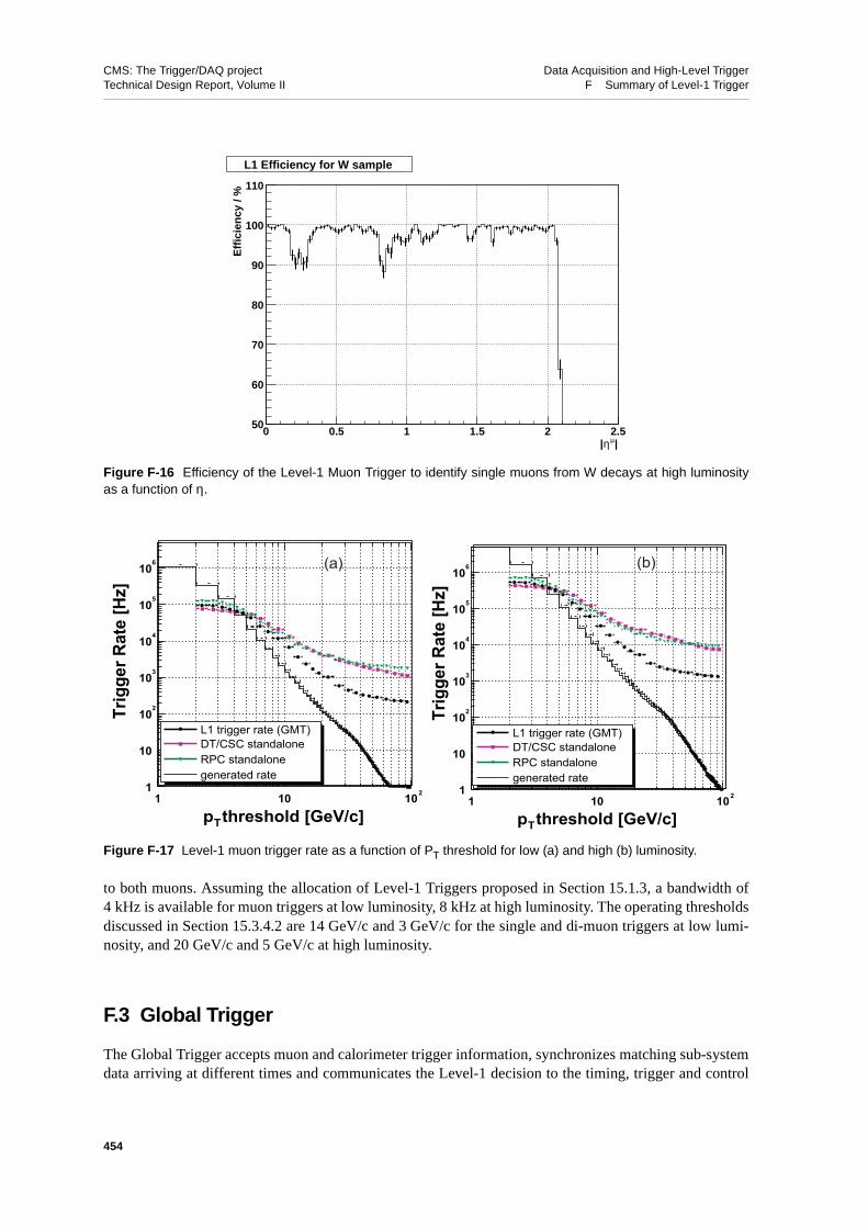
CMS: The Trigger/DAQ project Data Acquisition and High-Level TriggerTechnical Design Report, Volume II F Summary of Level-1 Trigger
to both muons. Assuming the allocation of Level-1 Triggers proposed in Section 15.1.3, a bandwidth of4 kHz is available for muon triggers at low luminosity, 8 kHz at high luminosity. The operating thresholdsdiscussed in Section 15.3.4.2 are 14 GeV/c and 3 GeV/c for the single and di-muon triggers at low lumi-nosity, and 20 GeV/c and 5 GeV/c at high luminosity.
F.3 Global Trigger
The Global Trigger accepts muon and calorimeter trigger information, synchronizes matching sub-systemdata arriving at different times and communicates the Level-1 decision to the timing, trigger and control
Figure F-16 Efficiency of the Level-1 Muon Trigger to identify single muons from W decays at high luminosityas a function of η.
Figure F-17 Level-1 muon trigger rate as a function of PT threshold for low (a) and high (b) luminosity.
|µη|0 0.5 1 1.5 2 2.5
Eff
icie
ncy
/ %
50
60
70
80
90
100
110
L1 Efficiency for W sample
threshold [GeV/c]Tp1 10 102
Trig
ger R
ate
[Hz]
1
10
102
103
104
105
106
L1 trigger rate (GMT)DT/CSC standaloneRPC standalonegenerated rate
threshold [GeV/c]Tp1 10 102
Trig
ger R
ate
[Hz]
1
10
102
103
104
105
106
L1 trigger rate (GMT)DT/CSC standaloneRPC standalonegenerated rate
(a) (b)
454
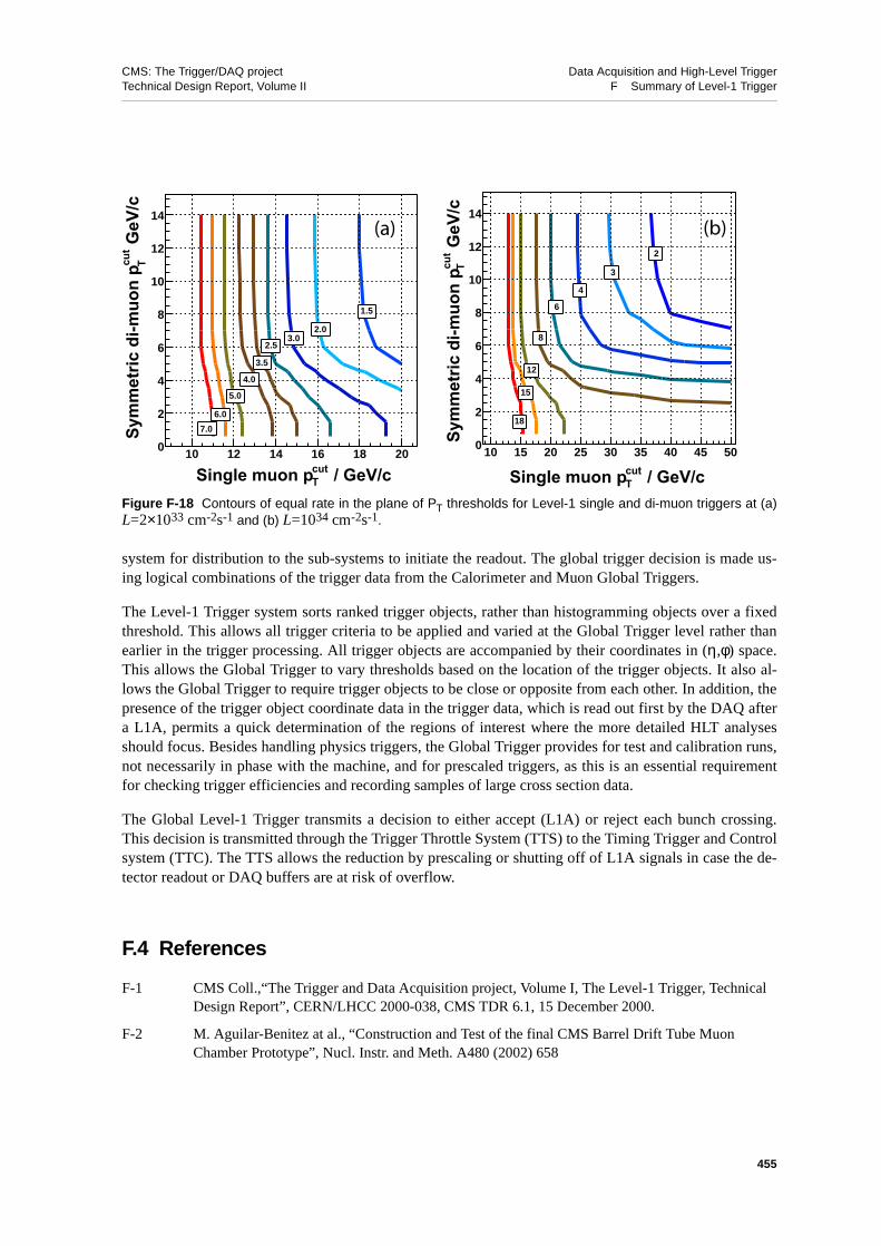
CMS: The Trigger/DAQ project Data Acquisition and High-Level TriggerTechnical Design Report, Volume II F Summary of Level-1 Trigger
system for distribution to the sub-systems to initiate the readout. The global trigger decision is made us-ing logical combinations of the trigger data from the Calorimeter and Muon Global Triggers.
The Level-1 Trigger system sorts ranked trigger objects, rather than histogramming objects over a fixedthreshold. This allows all trigger criteria to be applied and varied at the Global Trigger level rather thanearlier in the trigger processing. All trigger objects are accompanied by their coordinates in (η,φ) space.This allows the Global Trigger to vary thresholds based on the location of the trigger objects. It also al-lows the Global Trigger to require trigger objects to be close or opposite from each other. In addition, thepresence of the trigger object coordinate data in the trigger data, which is read out first by the DAQ aftera L1A, permits a quick determination of the regions of interest where the more detailed HLT analysesshould focus. Besides handling physics triggers, the Global Trigger provides for test and calibration runs,not necessarily in phase with the machine, and for prescaled triggers, as this is an essential requirementfor checking trigger efficiencies and recording samples of large cross section data.
The Global Level-1 Trigger transmits a decision to either accept (L1A) or reject each bunch crossing.This decision is transmitted through the Trigger Throttle System (TTS) to the Timing Trigger and Controlsystem (TTC). The TTS allows the reduction by prescaling or shutting off of L1A signals in case the de-tector readout or DAQ buffers are at risk of overflow.
F.4 References
F-1 CMS Coll.,“The Trigger and Data Acquisition project, Volume I, The Level-1 Trigger, Technical Design Report”, CERN/LHCC 2000-038, CMS TDR 6.1, 15 December 2000.
F-2 M. Aguilar-Benitez at al., “Construction and Test of the final CMS Barrel Drift Tube Muon Chamber Prototype”, Nucl. Instr. and Meth. A480 (2002) 658
Figure F-18 Contours of equal rate in the plane of PT thresholds for Level-1 single and di-muon triggers at (a)L=2×1033 cm-2s-1 and (b) L=1034 cm-2s-1.
/ GeV/ccutTSingle muon p
10 12 14 16 18 20
GeV
/ccu
tT
Sym
met
ric d
i-muo
n p
0
2
4
6
8
10
12
14
7.0
6.0
5.0
4.0
3.5
3.02.5
2.0
1.5
/ GeV/ccutTSingle muon p
10 15 20 25 30 35 40 45 50 G
eV/c
cut
TSy
mm
etric
di-m
uon
p0
2
4
6
8
10
12
14
18
15
12
8
6
4
3
2
(a) (b)
455

CMS: The Trigger/DAQ project Data Acquisition and High-Level TriggerTechnical Design Report, Volume II F Summary of Level-1 Trigger
456

CMS: The Trigger/DAQ project Data Acquisition and High-Level TriggerTechnical Design Report, Volume II G Extending the Use of Tracking in the HLT
G Extending the Use of Tracking in the HLT
The systematic optimization of the track reconstruction code and the extensive use of “regional” and“conditional” track reconstruction, described in Section 14.4.3, allow fast and robust tagging and detailedcharacterization of electrons, muons and tau's, as well as of b-jets with displaced vertices, with sufficientspeed to be used for a large fraction of, and possibly the full, Level-1 event rate, at both low and high lu-minosity.
The optimization of track reconstruction in the HLT has made rapid progress in the past year, and is stillongoing. In what follows, ways in which extended use of track reconstruction may be applied to furtherimprove the CMS HLT filters are illustrated with a few specific examples.
The HLT strategy described below does not use the standard Level-2 muon selection and instead uses thepartial tracking algorithms described in Section 14.4.3. The main components are the same as the stan-dard track reconstruction: fast and efficient pixel reconstruction, aggressive track seed filtering using pri-mary vertex information and Level-1 muon trigger information; partial track reconstruction using filteredseeds. For B physics, vertex and mass constraints are then used for the final event selection, while forb-jet tagging, the corresponding tagging algorithm is used.
G.1 Benchmark Channels for Inclusive jet b-tagging
Final states which contain b-jets have been proposed as very promising Higgs discovery channels. In thissection the selection efficiencies using a b-tag right after the Level-1 selection for two channels is studied:
• WH→µνbb, with a Higgs mass of 115 GeV/c2, triggered at Level-1 by a high-PT muon
• fully hadronic decays of ttH→bjjbjjbb, with a Higgs mass of 120 GeV/c2
The cross sections and rates of these channels, together with those of the main backgrounds expected, aregiven in Table G-1. The main process which contributes to the rate for the first channel derives from theWjj→µjjX production, in which the muon can come either from the direct leptonic W decay as well asfrom other muons present in the event, such as for instance c-quark semi-leptonic decays. This processhas a cross section of about 16 nb. Despite the larger cross section, the Z/γ→µjjX process has less impactdue to its softer muon PT spectrum. For the ttH channel the main background arises from QCD jets. Thisbackground can be reduced by requiring the presence of at least two or three identified b-jets.
G.1.1 WH with H Decaying to Jets
The study has been performed at low luminosity for the staged pixel detector case. Events are triggered atLevel-1 by a muon with PT>10 GeV/c at least two Level-1 jets with ET>20 GeV and |η|<5, giving a totalrate of 2.2 kHz. A muon track is then searched for directly in the tracker using a regional approach. Re-gional seeds are made of combinations of pixel hits in a cone of size |∆η|<0.1 and ∆φ<0.3 around the Lev-el-1 muon direction, centered in the origin with a tolerance of 15 cm along the z direction, a maximum 2Dimpact parameter of 100 µm and a PT>10 GeV/c. For the signal events there is almost always a singlecandidate track and the efficiency to find such a track is about 90%. The muon track z impact point de-fines the z coordinate for the primary vertex of the event with 50 µm precision. Muon isolation is then re-quired: tracks with PT>1 GeV/c are reconstructed within a cone of |∆η|<0.2 and ∆φ<0.2 around the muondirection, compatible from coming within a cylinder of 1 mm diameter and length, centered on the previ-ously found primary vertex. The event is rejected if the PT sum of the tracks found, excluding the muon
457

CMS: The Trigger/DAQ project Data Acquisition and High-Level TriggerTechnical Design Report, Volume II G Extending the Use of Tracking in the HLT
track, exceeds 3 GeV/c. The time for the two above steps is less than 150 ms on an Intel 1 GHz Pen-tium-III CPU. Two calorimetric jets are further required to be within the tracker acceptance. Tracks ofPT>2 GeV/c and a maximum of 7 hits are then reconstructed in cone of ∆η<0.4 and ∆φ<0.4 around the jetdirections and compatible with coming from the primary vertex. A simple b-tag algorithm is applied tothe jets, as outlined in Section 15.6.1, which requires two tracks with a 2D impact parameter significancelarger than 2. The time to reconstruct those tracks and apply the b-tag is about 130 ms per jet. Details canbe found in reference [G-1].
The main background comes from QCD events in which at least one muon triggered the Level-1 selec-tion. Figure G-1 shows the rate for minimum-bias events and the efficiency for the signal events as afunction of the single muon threshold as measured by the muon Level-1. Already at this stage, for a muonPT threshold of 15 GeV/c, the background rate is decreased from 2.7 kHz to about 1.6 Hz while a globalefficiency of 13% for at least one b-jet tagged is maintained.
The above selection is also very efficient for top-quark semileptonic decays and can be used as an alterna-tive with respect to the inclusive single-muon selection described in Section 15.3.3, if two calorimetricjets are present. In particular, taking into account that the Wjj cross section with two jets with ET>15 GeVwithin the tracker acceptance is about one third of the inclusive W cross section, the use of the above se-lection might allow to redirect the muon HLT resources to other interesting channels [G-1].
G.1.2 ttH Fully Hadronic Decays
Final states containing many b-jets have an enormous background from QCD multi jet production. Whena muon from the W decay is present, this channel can be easily selected at trigger level. Nevertheless, pre-liminary studies have shown [G-2] a valuable increase in the discovery potential by using in addition thefully hadronic ttH decays, which instead must be triggered against the large QCD background.
Table G-1 Cross sections and rates for different final states, together with the kinematic cuts applied at genera-tion level.
Process
Kinematic cutsCross
section
Rate at 2×1033 cm-2 s-1
(Hz)PT
µ
(GeV/c)|ηµ|
PThard
(GeV/c)
WH→µνbb 0.131 pb 2.62 10-4
ttH→bjjbjjbb 0.36 pb 7.2 10-4
Wjj→µjjX >3 <2.5 16 nb 32.5
Z/γ→µjjX >3 <2.5 22 nb 44.2
QCD 1 GeV/c< PTµ< 4 GeV/c 1 - 4 <2.5 15-50, >170 17 µb 34 103
QCD 4 GeV/c< PTµ< 10 GeV/c 4 - 10 <2.5 15-50, >170 9.8 µb 20 103
QCD PTµ> 10 GeV/c >10 <2.5 15-50, >170 0.53 µb 1.1 103
QCD 0<PThard<15 0 - 15 52.4 mb 1 108
QCD 50<PThard<80 50 - 80 24 µb 48 103
QCD 80<PThard<120 80 - 120 3.4 µb 6.8 103
QCD 120<PThard<170 120 - 170 0.57 µb 1.1 103
458

CMS: The Trigger/DAQ project Data Acquisition and High-Level TriggerTechnical Design Report, Volume II G Extending the Use of Tracking in the HLT
At Level-1 events are selected using a calorimetric jet trigger. The efficiency for this channel at Level-1,as a function of the cut on the calibrated jet ET, for jets with |η| < 2.5, is shown in Figure G-2 (left). It ispossible to achieve 25% efficiency on the signal by requiring 4 jets with ET >75 GeV and a rate, at low lu-minosity, of ~10 Hz (Figure 15-39).
The HLT selection requires a number of jets to be identified as b-jets. The jets are preselected requiringET>50 GeV. The primary vertex is reconstructed using pixel lines with PT>2 GeV/c. The region of inter-est is defined as a cone of 0.4 around the jet direction, while partial track reconstruction stops when givehits are found. The b-tag algorithm is the one described in Section 15.6, which requires two tracks withlarge significance on the transverse impact parameter measurement. Figure G-2 (right) shows the effi-ciency for the signal selection versus the background rate, at low luminosity, for different cuts on thetransverse impact parameter significance of the track. It is possible to reduce the QCD rate to about 10 Hzrequiring a b-tag on the leading jet with 50% of signal efficiency [G-3].
Figure G-1 Rate for minimum-bias events (left) and efficiency for signal events (right) as a function of the singlemuon threshold as measured by the muon Level-1 Trigger.
Figure G-2 Efficiency to select ttH events. On the left: as a function of the calibrated jet ET of the first four jetswithin the tracker acceptance. On the right: as a function of the QCD rate. The two curves show the effect ofb - tagging at least one jet or at least two jets in the event. The different points refer to different b - tag condi-tions.
L=2x1033cm-2s-1 staged Pixel [7 hits]
L1 ptµ [GeV/c]
Rat
e [H
z] 1 Isolated Muon and 2 jets Et cor>20 GeV |η|<5
+ 2 central leading jets + at least 1 jet b-tagged
10-1
1
10
10 2
10 3
10 4
10 15 20 25 30 35
L=2x1033cm-2s-1 staged Pixel [7 hits]
L1 ptµ [GeV/c]
Sele
ctio
n Ef
ficie
ncy
W(→
µν)H
(→bb
-- )
1000 evts/year
500 evts/year
100 evts/year
1 Isolated Muon and 2 jets Et cor>20 GeV |η|<5
+ 2 central leading jets + at least 1 jet b-tagged
0
0.1
0.2
0.3
0.4
0.5
0.6
10 15 20 25 30 35
0
0.2
0.4
0.6
0.8
1
0 25 50 75 100 125 150 175 200 225 250
1 jets 2 jets 3 jets
Calibrated jet ET (GeV)
Sel
ectio
n E
ffici
ency
ttH
4 jets
0
0.1
0.2
0.3
0.4
0.5
0.6
0.7
0.8
0.9
1
1 10 102
103
QCD Rate (Hz)
Sel
ectio
n E
ffici
ency
ttH
At Least 1 b-Tagged Jet
At Least 2 b-Tagged Jet
At Least 4 Jets with ET> 50(GeV)
459

CMS: The Trigger/DAQ project Data Acquisition and High-Level TriggerTechnical Design Report, Volume II G Extending the Use of Tracking in the HLT
G.2 Exclusive B-physics Triggers
Due to the large bb cross section, even a fully efficient b-tag cannot retain all b-hadron decays to allowthe selection of exclusive decays. Instead such decays must be reconstructed within the large background.The B-physics selection is triggered at Level-1 by the presence of one or two muons. The aim of the HLTselection is to reconstruct the decays either of the associated b hadron or those of the two muons (such asin the case of the J/ψ decays), by using invariant mass and displaced vertices cuts.
Results on three channels, whose selection relies on track reconstruction after a Level-1 muon trigger areshown:
• Bs→J/ψφ→µµΚΚ
• Bs→µµ
• b→µ+Bs →π Ds→φ(ΚΚ)π.
From the results of the first and second channel, an inclusive trigger path for J/ψ→µµ is also derived.
Table G-2 lists the data samples used for the signal and background. To save CPU time, events were gen-erated and selected with the following requirements:
• within the Pythia generator the PThard of the hard interaction has to be larger than 1 GeV/c;
• in the case of the fully hadronic channel, one b-hadron is forced to decay into a muon;
• The second b-hadron is forced to decay via the signal channel, and its decay products are requiredto satisfy the PT cuts listed in Table G-2.
The algorithms for the reconstruction of the primary vertex and charged particle tracks were developedfor inclusive jets are thus not optimal for use with the relatively low-ET b-jets involved in typical B sam-ples. In particular, the minimum PT of the decay tracks needs to be reconstructed from about 700 MeV/c.In order to limit the large number of seeds for this low PT value only those seeds which are close to the zcoordinate of the interaction point that produced the bb pair are considered. The seeds are reconstructedusing the Fast Track seed generator based on pixel detectors.
G.2.1 B Decays to Muon Final States
Events are triggered at Level-1 requiring at least two muon candidates with PT>4 GeV/c and oppositecharge. Two slightly different trigger strategies for Bs →µµ and Bs→J/ψφ are described below.
Table G-2 Cuts at generator level and cross sections for the samples used.
Kinematic cuts Bs→J/ψ φ→µµΚΚ Bs→µµb→µ+Bs→ πDs→φ(ΚΚ)π
Inclusive muon sample
pµT,ph
T,|η| 2 GeV/c, 0.5 GeV/c, 2.5 2 GeV/c, -,2.5 4 GeV/c, 0.5 GeV/c, 2.5
4 GeV/c
cross section (fb) 97 103 92 13 103 24 1012
460

CMS: The Trigger/DAQ project Data Acquisition and High-Level TriggerTechnical Design Report, Volume II G Extending the Use of Tracking in the HLT
G.2.1.1 Bs → µµ Selection
Events are required to have two oppositely-charged isolated muons coming from a common displacedvertex and having an invariant di-muon mass close to the nominal Bs mass. At a first stage, the fast seedgenerator reconstructs all pixel hit pairs which can be assigned to the tracks with PT > 4 GeV/c and trans-verse impact parameter smaller than 0.1 cm. The reconstructed track pairs are used for a first reconstruc-tion of the primary vertex. The three most significant primary vertices are retained per event. At a secondstage hit pairs are filtered using the vertex constraint and the regions defined by the Level-1 muons(∆η<0.5 and ∆φ<0.8 ± 0.4 correction). Filtered hit pairs are then used for the reconstruction of tracks.This reconstruction is stopped when one of the following three conditions are met: (a) the track PT is low-er than 4 GeV/c at 5 σ, or (b) 6 hits along the trajectory are found, or if (c) the relative resolution on PT issmaller than 2%. The reconstructed tracks are back propagated to the origin using the standard smoothingprocedure. If and only if two opposite charged tracks are reconstructed, the algorithm checks the invariantmass which has to be in 150 MeV/c2 from the Bs mass (Figure G-3). In order to suppress combinatorial
background, tracks are vertexed and retained if the χ2 is smaller than 20 and the decay length distance inthe transverse plane is larger than 150 µm. The algorithm described uses all the ingredients required bythe offline selection [G-4] but with much softer cuts to keep the useful events for further analysis. Theglobal selection efficiency on the signal events is 5% and the timing is on average 240 ms on a 1 GHz In-tel Pentium-III CPU, so it could be implemented at the HLT stage. The estimated background rate is be-low 2 Hz (Table G-3).
G.2.1.2 Bs → J/ψ φ→µµ ΚΚ Selection
Muons from J/ψ decays are reconstructed in the same way as for the ones of the Bs→µµ reconstruction,except the fact the a slightly tighter cuts on the di-muon mass and secondary vertex are required to keep
Figure G-3 Invariant mass distribution for Bs→µµ decays. Left: in the HLT; right: offline reconstruction.
Table G-3 Trigger efficiencies, number of events/10 fb-1 and background rate for Bs → µµ reconstruction (seetext). The global efficiency is the efficiency of the combined Level-1 and HLT selections.
L1 Trigger Efficiency HLT efficiency Global Efficiency Events/10 fb-1 Trigger Rate
15.2% 33.5% 5.1% 47 <1.7 Hz
461

CMS: The Trigger/DAQ project Data Acquisition and High-Level TriggerTechnical Design Report, Volume II G Extending the Use of Tracking in the HLT
the background rate at acceptable level. The mass window is decreased to 100 MeV/c2 (Figure G-4) andthe secondary vertex has to be at least 200 µm from the beam with a vertex χ2 < 10.
This di-muon selection leads to an inclusive rate of about 15 Hz for low luminosity, 90% of which com-posed of J/ψ from b decays. This selection is sufficiently inclusive to allow further offline selections,such as identifying J/ψK0
s decays. This first stage takes on average 260 ms and can be run on every eventpassing the Level-1 Trigger. The full reconstruction of the Bs is more demanding in CPU time and there-fore must be run at Level-3 to reduce the rate below 1 Hz. To select the kaon tracks coming from the φmeson, all track seeds within a cone of ∆R<1.5 around the reconstructed J/ψ direction are reconstructedup to 6 hits or the relative uncertainty on PT becomes smaller than 2%. Charged tracks of opposite signare then paired and retained if the invariant mass is within 10 MeV/c2 of the φ mass. Once a candidate isfound the invariant mass of the J/ψ and φ system is computed and the Bs candidate is retained if it fallswithin 60 MeV/c2 of the Bs mass. To further decrease the background, the Bs vertex is required to satisfyχ2<200.
Table G-4 shows the efficiencies and yields for signal events together with the rates from backgrounds atlow luminosity. The average execution time for signal and background events on a 1 GHz Intel Pen-tium-III CPU is about 260 ms for the reconstruction of the J/ψ and 800 ms for the reconstruction of thefull Bs, out of which about 400 ms is spent on the reconstruction of the φ.
G.2.1.3 b → µ + Bs → π + Ds→ φ(ΚΚ)π Selection
This study has been performed for low luminosity. The Level-1 Trigger is based either on a single muonor on the combination of a low-PT muon and a relatively ET jet. Table G-5 shows the expected triggerrates as a function of the different cuts on the muon and the soft jet. Table G-6 shows the yields for signalevents. The machine conditions and the instantaneous luminosity may well allow running the Level-1Trigger using lower thresholds than the nominal ones, which have been determined for a luminosity of for
Figure G-4 Mass resolutions for φ, J/ψ and Bs signal candidates.
Table G-4 Trigger efficiencies, number of events/10 fb-1 and background rate for Bs → J/ψ φ reconstruction.
Level-1 Muon Efficiency
Level-2 Efficiency Level-2 Rate
Level-3 Efficiency Level-3 Rate Events/10 fb-1
16.5% 13.7% 14.5 Hz 8.7% <1.7 Hz 83800
462

CMS: The Trigger/DAQ project Data Acquisition and High-Level TriggerTechnical Design Report, Volume II G Extending the Use of Tracking in the HLT
discovery. The HLT trigger strategy is based mainly on the reconstruction of the different resonances inthe decay.
The pixel primary vertex finder is reconstructed as in Section 14.4.2. Tracks are reconstructed withPT>0.7 GeV/c and with 3 hits only: two in the pixel detector and one in the first layer of the silicon detec-tor, to allow for sufficiently large lever arm. To reduce execution time, seeds are requested to come fromthe primary vertex z location ±1 mm. A search is then made for the φ, Ds and Bs candidates using the fol-lowing three requirements: ∆R(ΚΚ )<0.3, ∆R(φπ)<1.2 and ∆R(Dsπ)<3.0.
Figure G-5 shows the invariant mass resolutions for the φ, Ds and Bs candidates. The main cuts are basedon invariant mass and the pT of the three resonances. A 3D reconstruction of the Ds vertex is also per-formed. The details can be found in reference [G-4].
The signal efficiency after all these cuts is about 10%, while the background is suppressed by a factor250. The mean execution time for signal and background events, referred to a single 1 GHz Intel Pen-tium-III CPU, is 640 ms. The number of signal events will depend on the allowed bandwidth given to thischannel, according to the instantaneous luminosity of LHC. From the above tables even a relatively largethreshold of 14 GeV/c gives a rate of 3 kHz after Level-1. Since the allowed bandwidth would be lowerthan this, it is necessary to scale the rate, which can be either done scaling the rate of the lowest possiblemuon PT bin or scale each bin in PT such that the overall sum matches the allowed band. On the other
Table G-5 HLT (Level-1) rates, in kHz, as a function of the cuts on themuon and the jet.
Muon pT (GeV/c)
Rate (kHz)
ET>0 GeV ET>20 GeV ET>30 GeV
4 0.27 (50) 0.15 (15) 0.08 (5.7)
5 0.19 (33) 0.10 (11) 0.06 (4.2)
6 0.16 (26) 0.082 (8.5) 0.055 (3.6)
7 0.11 (18) 0.062 (6.2) 0.045 (2.7)
10 0.037 (6.4) 0.021 (2.5) 0.014 (1.3)
14 0.017 (3.2) 0.010 (1.3) 0.008 (0.7)
Table G-6 Number of signal events after HLT (Level-1) trigger as afunction for different values of the Level-1 selection cuts for an inte-grated luminosity of 20 fb-1.
Muon pT (GeV/c)
Number of events (1000)
ET>0 GeV ET>20 GeV ET>30 GeV
4 11K (106 K) 4.8 K (34 K) 2.3 K (14 K)
5 8 K (78 K) 3.6 K (28 K) 2 K (12 K)
6 7.4 K (65 K) 3.1 K (24 K) 1.5 K (11 K)
7 5.6 K (48 K) 2.4 K (20 K) 1.3 K (9.4 K)
10 2.0 K (20 K) 1.0 K (9.6 K) 0.6 K (5.3 K)
14 1K (11 K) 0.5 K (5.4 K) 0.3 K (3. K)
463

CMS: The Trigger/DAQ project Data Acquisition and High-Level TriggerTechnical Design Report, Volume II G Extending the Use of Tracking in the HLT
hand the quality of the analysis will depend on the total number of events, the fraction of signal eventsand their dilution factor [G-4]. By rising the muon PT the signal fraction and dilution increases mildly[G-5], while the total number of events decreases. Therefore it is better to fill the allowed bandwidth withevents with the lowest possible muon PT and downscale only the bin which would be needed for fillingthe band. For example, referring to Table G-5, for an allowed bandwidth of 5 kHz, all events with muonPT>14 GeV/c shoud be kept, while events with 10 GeV/c<PT<14 GeV/c should be scaled by a factor two.
G.3 References
G-1 R. Ranieri, “A High-Level Trigger Selection of WH→µνbb using the Tracker and b-jets”, CMS Note 2002/048.
G-2 V. Drollinger, PhD Thesis, IEKP, Karlsruhe University, Germany. CMS 2001-028/THESIS.
G-3 D. Benedetti, L. Fano, “Study of High Level b-trigger Selection of ttH Fully Hadronic Decays”, CMS Note 2002/044.
G-4 A. Giassi, F. Palla and A. Starodumov, “Study for a High-Level Trigger for the decay channel Bs→π +Ds→ φ(KK)ππ ”, CMS Note 2002/045.
G-5 Z. Xie, PhD Thesis, Scuola Normale Superiore, Pisa, Italy. CMS 2001-018/THESIS.
Figure G-5 Invariant mass distribution of φ, Ds and Bs candidates.
0
50
100
150
200
250
300
350
400
0.98 0.99 1 1.01 1.02 1.03 1.04 1.05 1.060
50
100
150
200
250
300
350
400
0.98 0.99 1 1.01 1.02 1.03 1.04 1.05 1.06
σ=5 MeV
M (GeV)
Arb
itrar
y un
its
0
25
50
75
100
125
150
175
200
225
1.8 1.85 1.9 1.95 2 2.05 2.1 2.15 2.20
25
50
75
100
125
150
175
200
225
1.8 1.85 1.9 1.95 2 2.05 2.1 2.15 2.2
σ=25 MeV
MDs (GeV)
Arb
itrar
y un
its
0
10
20
30
40
50
60
70
80
5.1 5.2 5.3 5.4 5.5 5.6 5.70
10
20
30
40
50
60
70
80
5.1 5.2 5.3 5.4 5.5 5.6 5.7
σ=95 MeV
MBs (GeV)
Arb
itrar
y un
its
464

CMS: The Trigger/DAQ project Data Acquisition and High-Level TriggerTechnical Design Report, Volume II CMS Trigger/DAQ project: Members and Contributors
CMS Trigger/DAQ project: Members and Contributors
Current participants in the CMS TriDAS Collaboration, as well as contributors to the High-Level Trigger, by Country and Institute.
Institut für Hochenergiephysik der OeAW, Wien, AUSTRIAW. Adam, H. Bergauer, C. Deldicque, J. Erö, R. Fruehwirth, A. Jeitler, K. Kastner, S. Kostner, N. Neumeister1, M. Padrta, P. Porth, H. Rohringer, H. Sakulin, J. Strauss, A. Taurok, G. Walzel, C.-E. Wulz
Vrije Universiteit Brussel, Brussel, BELGIUMS. Lowette, B. Van De Vyver1
Université Libre de Bruxelles, Bruxelles, BELGIUMG. De Lentdecker, P. Vanlaer
Université Catholique de Louvain, Louvain-la-Neuve, BELGIUMC. Delaere, V. Lemaitre, A. Ninane, O. van der Aa
Institute for Nuclear Research and Nuclear Energy, Sofia, BULGARIAJ. Damgov
Helsinki Institute of Physics, Helsinki, FINLANDK. Banzuzi, V. Karimäki, R. Kinnunen, T. Lampén, K. Lassila-Perini, V. Lefébure1, J. Nysten, E. Pietarinen2, D. Ungaro, M. Voutilainen
Laboratoire Leprince-Ringuet, Ecole Polytechnique, IN2P3-CNRS, Palaiseau, FRANCEP. Busson
Institut de Recherches Subatomiques, IN2P3-CNRS - ULP, LEPSI Strasbourg, UHA Mulhouse, Stras-bourg, FRANCET. Todorov
RWTH, I. Physikalisches Institut, Aachen, GERMANYB. Schwering
Institut für Experimentelle Kernphysik, Karlsruhe, GERMANYP. Gras
University of Athens, Athens, GREECEG. Daskalakis, A. Sfyrla
Institute of Nuclear Physics "Demokritos", Attiki, GREECEM. Barone, T. Geralis, C. Markou, K. Zachariadou
KFKI Research Institute for Particle and Nuclear Physics, Budapest, HUNGARYP. Hidas
Tata Institute of Fundamental Research - EHEP, Mumbai, INDIAS. Banerjee, K. Mazumdar1
Tata Institute of Fundamental Research - HECR, Mumbai, INDIAS. Banerjee
Università di Bari, Politecnico di Bari e Sezione dell' INFN, Bari, ITALYM. Abbrescia, A. Colaleo, M. D’Amato, N. De Filippis, D. Giordano, F. Loddo, M. Maggi, L. Silvestris, G. Zito
Università di Bologna e Sezione dell' INFN, Bologna, ITALYS. Arcelli, D. Bonacorsi, P. Capiluppi, G.M. Dallavalle, A. Fanfani, C. Grandi, S. Marcellini, A. Montanari, F. Odorici, R. Travaglini
Università di Catania e Sezione dell' INFN, Catania, ITALYS. Costa, A. Tricomi
Università di Firenze e Sezione dell' INFN, Firenze, ITALYV. Ciulli, N. Magini, R. Ranieri
Laboratori Nazionali di Legnaro dell' INFN, Legnaro, ITALY (associated institute)L. Berti, M. Biasotto, M. Gulmini1, G. Maron, N. Toniolo, L. Zangrando
465

CMS: The Trigger/DAQ project Data Acquisition and High-Level TriggerTechnical Design Report, Volume II CMS Trigger/DAQ project: Members and Contributors
Università di Padova e Sezione dell' INFN, Padova, ITALYM. Bellato, U. Gasparini, S. Lacaprara, P. Ronchese, S. Ventura
Università di Perugia e Sezione dell' INFN, Perugia, ITALYD. Benedetti, M. Biasini, L. Fanò, L. Servoli
Università di Pisa, Scuola Normale Superiore e Sezione dell' INFN, Pisa, ITALYG. Bagliesi, T. Boccali, S. Dutta, S. Gennai, A. Giassi, F. Palla, G. Segneri, A. Starodumov3
Università di Roma I e Sezione dell' INFN, Roma, ITALYP. Meridiani, G. Organtini
Università di Torino e Sezione dell' INFN, Torino, ITALYN. Amapane, F. Bertolino, R. Cirio
Chonnam National University, Kwangju, KOREAJ.Y. Kim, I.T. Lim, K.J. Ma
Seoul National University, Seoul, KOREAK.K. Joo, B.J. Kim, S.B. Kim, I.H. Park
Sungkyunkwan University, Suwon, KOREAB.G. Cheon, Y.I. Choi
Kyungpook National University, Taegu, KOREAK. Cho, S.W. Ham, D.H. Kim, G.N. Kim, W.Y. Kim, J.Y. Lee, S.K. Oh, Y.D. Oh, S.R. Ro, D.C. Son
National Centre for Physics, Quaid-I-Azam University, Islamabad, PAKISTANA. Osman1
Institute of Experimental Physics, Warsaw, POLANDK. Bunkowski, M. Cwiok, W. Dominik, K. Doroba, M. Kazana, J. Krolikowski, I. Kudla, M. Pietrusinski, K. Pozniak8, W. Zabolotny8, P. Zych
Soltan Institute for Nuclear Studies, Warsaw, POLANDM. Górski, L. Goscilo, G. Wrochna, P. Zalewski
Laboratório de Instrumentação e Física Experimental de Partículas, Lisboa, PORTUGALR. Alemany-Fernandez, C. Almeida, N. Almeida, J. Da Silva, M. Santos, I. Teixeira, J.P. Teixeira, J. Varela, N. Vaz Cardoso
Joint Institute for Nuclear Research, Dubna, RUSSIAV. Konoplyanikov, A. Urkinbaev
Institute for Nuclear Research, Moscow, RUSSIAA. Toropin4
Institute for Theoretical and Experimental Physics, Moscow, RUSSIAV. Gavrilov, V. Kolosov, A. Krokhotine, A. Oulianov, N. Stepanov
Moscow State University, Moscow, RUSSIAO.L. Kodolova1, I. Vardanyan
Vinca Institute of Nuclear Sciences, Belgrade, SERBIAJ. Ilic, G. Skoro
Universidad Autónoma de Madrid, Madrid, SPAINC. Albajar, J.F. Trocóniz
Instituto de Física de Cantabria (IFCA), CSIC-Universidad de Cantabria, Santander, SPAINA. Calderon, M.A. Lopez Virto, R. Marco, C. Martinez Rivero, F. Matorras, I. Vila
Universität Basel, Basel, SWITZERLANDS. Cucciarelli, M. Konecki
CERN, European Organization for Nuclear Research, Geneva, SWITZERLANDS. Ashby, D. Barney, P. Bartalini, R. Benetta, V. Brigljevic, G. Bruno, E. Cano, S. Cittolin, A. Csilling, A. De Roeck, P. Favre, A. Frey, W. Funk, D. Futyan, D. Gigi, F. Glege, J. Gutleber, M. Hansen, V. Innocente, C. Jacobs, W. Jank, M. Kozlovszky, H. Larsen, M. Lenzi, I. Magrans, M. Mannelli, F. Meijers, E. Meschi, L. Mirabito5, S.J. Murray, A. Oh, L. Orsini, C. Palomares Espiga, L. Pollet, A. Racz, S. Reynaud, D. Samyn, P. Scharff-Hansen, C. Schwick, G. Sguazzoni, N. Sinanis, P. Sphicas6, A. Strandlie, B.G. Taylor, I. Van Vulpen,
466

CMS: The Trigger/DAQ project Data Acquisition and High-Level TriggerTechnical Design Report, Volume II CMS Trigger/DAQ project: Members and Contributors
J.P. Wellisch, M. Winkler
Paul Scherrer Institut, Villigen, SWITZERLANDD. Kotlinski
Universität Zürich, Zürich, SWITZERLANDK. Prokofiev, T. Speer
Cukurova University, Adana, TURKEYI. Dumanoglu
University of Bristol, Bristol, UNITED KINGDOMD.S. Bailey, J.J. Brooke, D. Cussans, G.P. Heath, D. Machin, S.J. Nash, D.M. Newbold, M.G. Probert
Rutherford Appleton Laboratory, Didcot, UNITED KINGDOMJ.A. Coughlan, R. Halsall, W.J. Haynes, I.R. Tomalin
Imperial College, University of London, London, UNITED KINGDOMN. Marinelli, A. Nikitenko3, S. Rutherford, C. Seez1
Brunel University, Uxbridge, UNITED KINGDOMO. Sharif
University of California, Davis, Davis, California, USAR. Breedon, P.T. Cox, P. Murray, M. Tripathi
University of California, San Diego, La Jolla, California, USAS. Bhattacharya, J.G. Branson, I. Fisk, J. Letts, M. Mojaver, H.P. Paar, E. Trepagnier
University of California, Los Angeles, Los Angeles, California, USAR. Cousins, S. Erhan, J. Hauser, P. Kreuzer, M. Lindgren, J. Mumford, P. Schlein, Y. Shi, B. Tannenbaum, V. Valuev, M. Von Der Mey
California Institute of Technology, Pasadena, California, USAV. Litvine, S. Shevchenko, R. Wilkinson
University of California, Riverside, Riverside, California, USAI. Andreeva1, R. Clare, S. Villa
University of Florida, Gainesville, Florida, USAD. Acosta, D. Bourilkov7, A. Korytov, A. Madorsky, G. Mitselmakher, J.L. Rodriguez, B. Scurlock
Fermi National Accelerator Laboratory, Batavia, Illinois, USAS. Aziz, M. Bowden, J.E. Elias, G. Graham, D. Green, M. Litmaath, V. O’Dell, N. Ratnikova, I. Suzuki, H. Wenzel
University of Maryland, College Park, Maryland, USAS. Abdullin3, D. Baden, S.C. Eno, T. Grassi, S. Kunori
Boston University, Boston, Massachusetts, USAG. Antchev7, E. Hazen, J. Rohlf, S. Wu
Northeastern University, Boston, Massachusetts, USAI. Osborne, L. Taylor, L. Tuura
Massachusetts Institute of Technology, Cambridge, Massachusetts, USAS. Pavlon, K. Sumorok, S. Tether
University of Mississippi, University, Mississippi, USAL.M. Cremaldi, D. Sanders, D. Summers
Princeton University, Princeton, New Jersey, USAW.C. Fisher, J. Mans, D. Stickland, C. Tully, T. Wildish, S. Wynhoff
Rice University, Houston, Texas, USAB.P. Padley
University of Wisconsin, Madison, Wisconsin, USAP. Chumney, S. Dasu, F.R. Di Lodovico, M. Jaworski, J. Lackey, W.H. Smith
467

CMS: The Trigger/DAQ project Data Acquisition and High-Level TriggerTechnical Design Report, Volume II CMS Trigger/DAQ project: Members and Contributors
1: Also at CERN, European Organization for Nuclear Research, Geneva, Switzerland 2: Now at Department of Physical Sciences, University of Helsinki, Finland 3: Also at Institute for Theoretical and Experimental Physics, Moscow, Russia 4: Also at Università di Pisa, Scuola Normale Superiore e Sezione dell' INFN, Pisa, Italy 5: Also at Institut de Physique Nucléaire de Lyon, IN2P3-CNRS, Univ. Lyon I, Villeurbanne, France 6: Also at MIT, Cambridge, USA and University of Athens, Greece 7: Also at Institute for Nuclear Research and Nuclear Energy, Sofia, Bulgaria8: Also at Institute of Electronic Systems, Technical University of Warsaw, Poland
468