IOP PUBLISHING SMART MATERIALS AND STRUCTURES

Smart Mater. Struct. 17 (2008) 065023 (12pp) doi:10.1088/0964-1726/17/6/065023

The application of statistical patternrecognition methods for damage detectionto field dataA Cheung1, C Cabrera1, P Sarabandi1, K K Nair1, A Kiremidjian1

and H Wenzel2

1 Department of Civil and Environmental Engineering, Stanford University, MC 4020,Stanford, CA 94305-4020, USA2 VCE Holding GmbH, Hadikgasse 60, A-1140 Wien, Austria

E-mail: cheunga@stanford.edu, ccabrera@stanford.edu, psarabandi@stanford.edu,kknair@stanford.edu, ask@stanford.edu and Wenzel@vce.at

Received 31 January 2008, in final form 12 September 2008Published 30 October 2008Online at stacks.iop.org/SMS/17/065023

AbstractRecent studies in structural health monitoring have shown that damage detection algorithmsbased on statistical pattern recognition techniques for ambient vibrations can be used tosuccessfully detect damage in simulated models. However, these algorithms have not beentested on full-scale civil structures, because such data are not readily available. A uniqueopportunity for examining the effectiveness of these algorithms was presented when data weresystematically collected from a progressive damage field test on the Z24 bridge in Switzerland.This paper presents the analysis of these data using an autoregressive algorithm for damagedetection, localization, and quantification. Although analyses of previously obtainedexperimental or numerically simulated data have provided consistently positive diagnosisresults, field data from the Z24 bridge show that damage is consistently detected, however notwell localized or quantified, with the current diagnostic methods. Difficulties with datacollection in the field are also revealed, pointing to the need for careful signal conditioning priorto algorithm application. Furthermore, interpretation of the final results is made difficult due tothe lack of detailed documentation on the testing procedure.

(Some figures in this article are in colour only in the electronic version)

1. Introduction

Structural health monitoring (SHM) for civil engineeringapplications is taking advantage of the latest technologiesin sensors, wireless networks, and data analysis methodsto protect civil infrastructure and preserve safety. SHMconsists of damage diagnosis and residual life prognosis.The goal of damage diagnosis is to detect, localize, andquantify structural damage arising from a variety of sources,including long-term degradation such as corrosion and short-term events such as earthquakes, and then to inform decision-makers about the proper responsive action. Interest in usingwireless sensing networks for structural health monitoring hasincreased as more research demonstrates successful applicationto increasingly complex structures. Wireless networks aredesirable, because they are cheaper and easier to install and

maintain than equivalent wired networks. However, theyrequire that the power consumption be minimal thus making itnecessary to limit data transmission (Straser and Kiremidjian1998).

One method of detecting damage in a structure isby measuring the structural response through strain oracceleration. The premise is that changes to structuralproperties caused by damage will change the way a structureresponds to any excitation, including ground motions.Vibration based damage detection methods have traditionallybeen based on system identification techniques (Doeblinget al 1996). Recent research has shown that statistical signalprocessing and pattern recognition techniques can be usedto diagnose damage successfully. Worden et al (1999) usedthe Mahalanobis distance to identify damage applying outlier

0964-1726/08/065023+12$30.00 © 2008 IOP Publishing Ltd Printed in the UK1

Smart Mater. Struct. 17 (2008) 065023 A Cheung et al

analysis. Their work was followed by several papers by Farrarand Sohn (2000), Sohn et al (2001a, 2001b), Farrar et al(2004, 2005), Worden et al (2003), Manson et al (2003a,2003b) Nair et al (2006) and Nair and Kiremidjian (2007). Theadvantage of using statistical methods is that a single vibrationtime history can be analyzed independently of all other signalscollected elsewhere in the structure. This allows damagedetection algorithms to be embedded at the sensor level,resulting in significant savings in power and computationaltime, both of which are necessary for the implementation ofa fully wireless network. This method has been successfullyapplied to numerically simulated damage to an experimentalstructure, such as the ASCE Benchmark Structure (Nair et al2006). However, computer simulations and even small-scalelaboratory test structures cannot fully duplicate the dynamicresponse of actual structures. More importantly, the inputambient vibrations imposed on actual structures are much morerandom and unpredictable than those used in most computerand laboratory simulations.

In order to test the effectiveness of damage detectionalgorithms on actual structures a suitable experiment must bedesigned. Such an experiment either requires a full or near full-scale test involving large facilities or an actual structure thatcan be subjected to controlled damage tests. For this reason,suitable experimental data are difficult to find. However,recent progressive damage tests performed on the Z24 bridgein Switzerland provide a large amount of experimental datawith which damage detection algorithms can be tested (Wenzel2005).

The purpose of this study is to test the robustness ofthe damage detection algorithm based on autoregressive timeseries modeling and statistical pattern recognition techniques,which were developed by Nair et al (2006), Nair andKiremidjian (2007), and Sohn et al (2001a, 2001b) in detectingand quantifying structural damage induced by pier settlement,using acceleration data from the Z24 bridge progressivedamage test. In addition, several modifications have beenmade to the original algorithm to enable more robust diagnosis.In particular, during the analysis of the data, it was foundthat a cumulative damage measure, which is the sum of theincremental damage measures between successive test cases,is able to characterize increasing damage in the form of piersettlement. This paper is organized in the following manner.First, the statistical pattern recognition methods for damagedetection are summarized. A new damage measure based onthe Mahalanobis distance is introduced. Next, the bridge anddata acquisition project are discussed. Finally, the cumulativedamage measure is introduced, and the results obtained fromtesting the algorithm on the Z24 bridge data are presented anddiscussed.

2. Overview of the damage detection algorithm

Statistical pattern recognition based damage detection algo-rithms are based on the hypothesis that a structure’s vibrationtime history will change with the onset of damage (Sohn et al2001a, 2001b, Nair et al 2006). Because the time historieshave complex signatures making them difficult to compare, it

is desirable to extract features from the signal referred to asdamage sensitive features (DSFs), with which damage can betracked. Nair et al (2006) have shown that decreases in a struc-ture’s stiffness due to damage will result in changes to AR co-efficients for acceleration time series collected under ambientvibrations. Thus AR coefficients are an appropriate DSF.

Damage is evaluated according to a pattern classificationframework. A pattern classification algorithm, accordingto Sohn et al (2001a, 2001b) involves the followingsteps: (i) evaluation of a structure’s operational environment,(ii) acquisition of structural response measurements and dataprocessing, (iii) extraction of features that are sensitiveto damage, and (iv) development of statistical models forfeature discrimination. In this study the structural responsemeasurements are acceleration time histories, and the DSFsare AR coefficients. Two methods for feature discriminationare proposed. Hypothesis testing using a t-test is performedas specified by Nair et al (2006); however it is shown thata normalized mean-difference value works just as well. Inaddition, a new multivariate damage measure (DM) basedon the Mahalanobis distance is proposed. The Mahalanobisdistance was used by Worden et al (1999) to determineoutliers in a signal for damage detection purposes. In thispaper the Mahalanobis distance is used to quantify damageextent. However, identifying damage location is complicatedand is beyond the scope of this paper. Each step in thedamage detection algorithm is explained in further detail in thefollowing sections.

3. Data preprocessing

Data preprocessing is done to remove or minimize dependenceon variable environmental conditions and to identify conditionswhere sensors have probably malfunctioned. Acceleration timeseries collected from field experiments often show a drift inthe signal. Linear drift is simple to correct. Nonlinear drift,however, is significantly more difficult to identify and correct(see Boore et al 2002). In this paper, time series exhibitingnonlinear drift were discarded while those exhibiting lineardrift were detrended. Linear drift can be removed by fittinga line to the signal using least squares methods and thensubtracting that line from the signal, thus removing the trend.

After detrending, additional preprocessing is doneto minimize the dependence on load and environmentalconditions. Sohn et al (2001a, 2001b) show that normalizingand standardizing the acceleration time history x(t) by

x(t) = (x(t) − μ)

σ(1)

where μ is the mean of the signal and σ is its standarddeviation, is required in order to minimize the effect of loadand environmental conditions on the AR coefficients. All timehistories examined in this study are filtered using equation (1)prior to application of the AR model.

As with all experiments, sensors may malfunction andproduce corrupt data. Review of the data collected atthe Z24 bridge show that 298 out of approximately 4000acceleration time histories collected during the test were

2

Smart Mater. Struct. 17 (2008) 065023 A Cheung et al

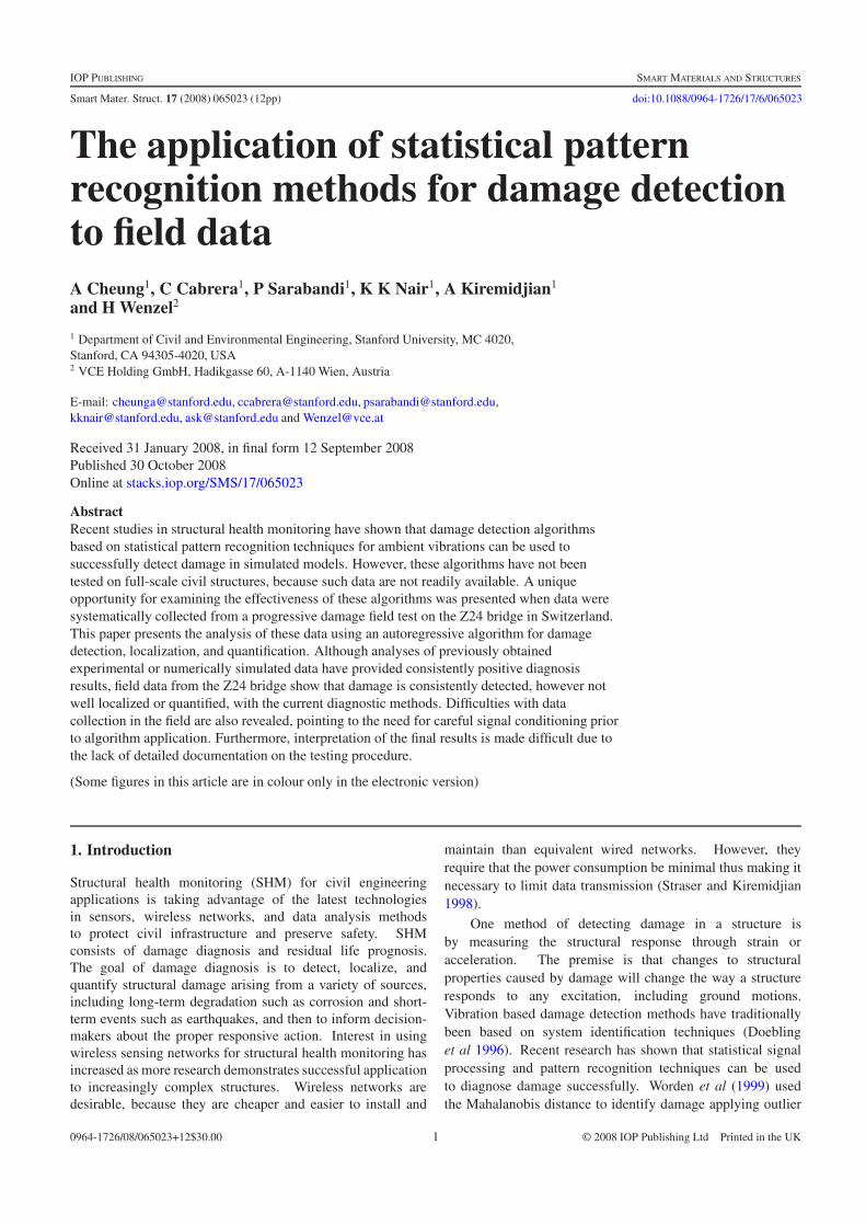
Figure 1. Example of corrupt time history.

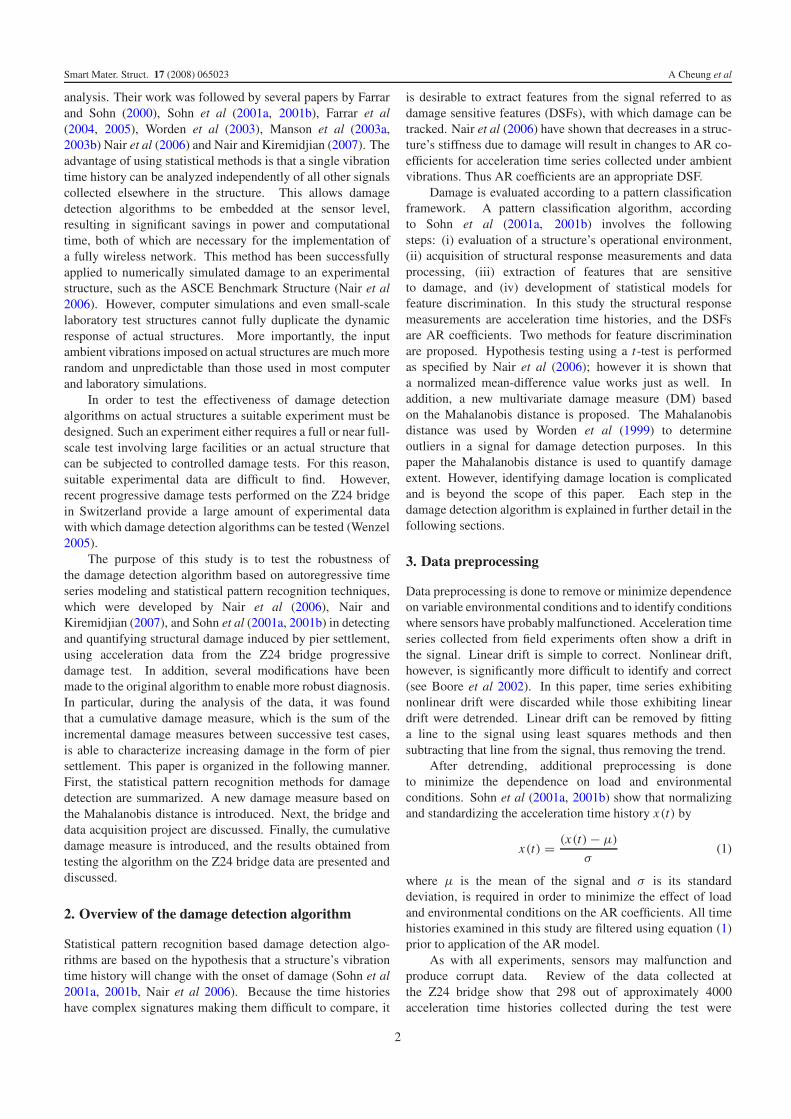
Figure 2. Example of corrupt time history.

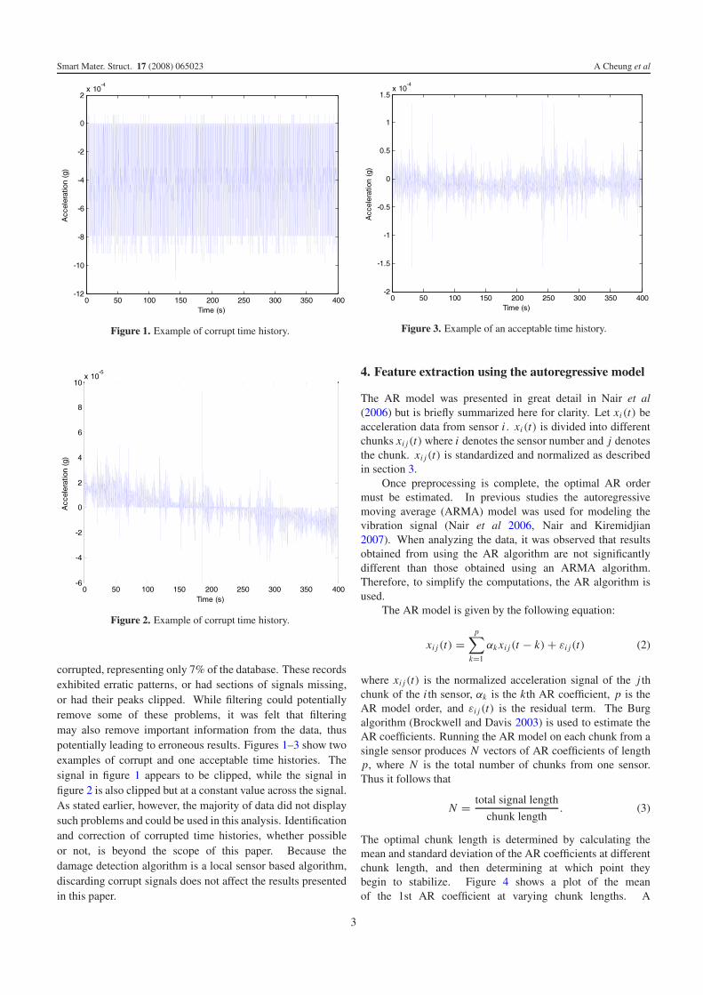
corrupted, representing only 7% of the database. These recordsexhibited erratic patterns, or had sections of signals missing,or had their peaks clipped. While filtering could potentiallyremove some of these problems, it was felt that filteringmay also remove important information from the data, thuspotentially leading to erroneous results. Figures 1–3 show twoexamples of corrupt and one acceptable time histories. Thesignal in figure 1 appears to be clipped, while the signal infigure 2 is also clipped but at a constant value across the signal.As stated earlier, however, the majority of data did not displaysuch problems and could be used in this analysis. Identificationand correction of corrupted time histories, whether possibleor not, is beyond the scope of this paper. Because thedamage detection algorithm is a local sensor based algorithm,discarding corrupt signals does not affect the results presentedin this paper.

Figure 3. Example of an acceptable time history.

4. Feature extraction using the autoregressive model

The AR model was presented in great detail in Nair et al(2006) but is briefly summarized here for clarity. Let xi(t) beacceleration data from sensor i . xi(t) is divided into differentchunks xi j(t) where i denotes the sensor number and j denotesthe chunk. xi j(t) is standardized and normalized as describedin section 3.

Once preprocessing is complete, the optimal AR ordermust be estimated. In previous studies the autoregressivemoving average (ARMA) model was used for modeling thevibration signal (Nair et al 2006, Nair and Kiremidjian2007). When analyzing the data, it was observed that resultsobtained from using the AR algorithm are not significantlydifferent than those obtained using an ARMA algorithm.Therefore, to simplify the computations, the AR algorithm isused.

The AR model is given by the following equation:

xi j(t) =p∑

k=1

αk xi j(t − k) + εi j(t) (2)

where xi j(t) is the normalized acceleration signal of the j thchunk of the i th sensor, αk is the kth AR coefficient, p is theAR model order, and εi j(t) is the residual term. The Burgalgorithm (Brockwell and Davis 2003) is used to estimate theAR coefficients. Running the AR model on each chunk from asingle sensor produces N vectors of AR coefficients of lengthp, where N is the total number of chunks from one sensor.Thus it follows that

N = total signal length

chunk length. (3)

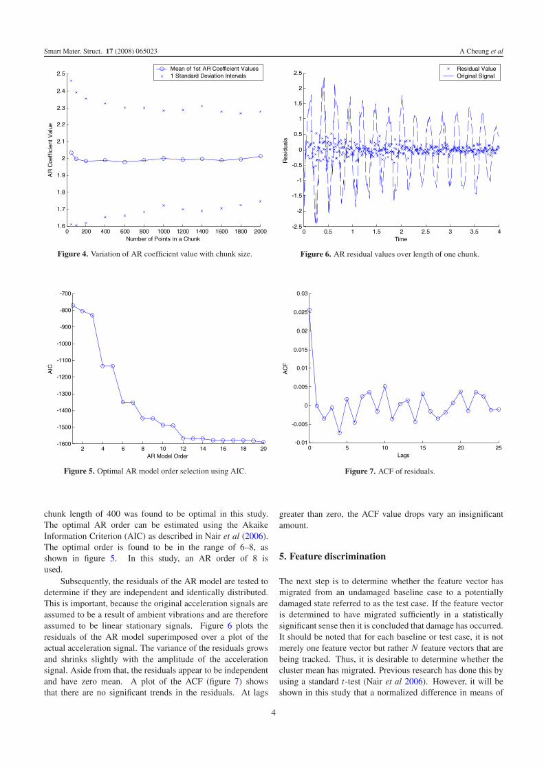
The optimal chunk length is determined by calculating themean and standard deviation of the AR coefficients at differentchunk length, and then determining at which point theybegin to stabilize. Figure 4 shows a plot of the meanof the 1st AR coefficient at varying chunk lengths. A

3

Smart Mater. Struct. 17 (2008) 065023 A Cheung et al

Figure 4. Variation of AR coefficient value with chunk size.

Figure 5. Optimal AR model order selection using AIC.

chunk length of 400 was found to be optimal in this study.The optimal AR order can be estimated using the AkaikeInformation Criterion (AIC) as described in Nair et al (2006).The optimal order is found to be in the range of 6–8, asshown in figure 5. In this study, an AR order of 8 isused.

Subsequently, the residuals of the AR model are tested todetermine if they are independent and identically distributed.This is important, because the original acceleration signals areassumed to be a result of ambient vibrations and are thereforeassumed to be linear stationary signals. Figure 6 plots theresiduals of the AR model superimposed over a plot of theactual acceleration signal. The variance of the residuals growsand shrinks slightly with the amplitude of the accelerationsignal. Aside from that, the residuals appear to be independentand have zero mean. A plot of the ACF (figure 7) showsthat there are no significant trends in the residuals. At lags

Figure 6. AR residual values over length of one chunk.

Figure 7. ACF of residuals.

greater than zero, the ACF value drops vary an insignificantamount.

5. Feature discrimination

The next step is to determine whether the feature vector hasmigrated from an undamaged baseline case to a potentiallydamaged state referred to as the test case. If the feature vectoris determined to have migrated sufficiently in a statisticallysignificant sense then it is concluded that damage has occurred.It should be noted that for each baseline or test case, it is notmerely one feature vector but rather N feature vectors that arebeing tracked. Thus, it is desirable to determine whether thecluster mean has migrated. Previous research has done this byusing a standard t-test (Nair et al 2006). However, it will beshown in this study that a normalized difference in means of

4

Smart Mater. Struct. 17 (2008) 065023 A Cheung et al

the baseline and test case suffice to show whether sufficientmigration has occurred.

In order to perform the calculations, however, the properdamage sensitive feature must first be formulated. As statedbefore, the DSF is a function of the AR coefficients, butdefining this function is not trivial. After extensive study ofthe data, it was observed that the first AR coefficient aloneis sufficient to capture the migration of the feature vectors.More complex combinations of AR coefficients tested did notsignificantly improve the performance of the algorithm.

The standard t-test can be used to determine whetherthe AR coefficient mean has changed significantly. The nullhypothesis H0 is that the AR coefficients from the base caseand test case are given by the same distribution. The t-statisticis calculated according to the following formula:

t = (μ2 − μ1)

Sp√

1n1

+ 1n2

(4)

Sp =√

(n1 − 1)σ 21 + (n2 − 1)σ 2

2

n1 + n2 − 2(5)

where μ1 and μ2 are the mean of the AR coefficients fromthe base case and test case, σ1 and σ2 are their standarddeviations, and n1 and n2 are the number of observations withineach group. Using the cdf of the t-distribution, p values arecalculated from the t-statistic, representing the probability ofobserving the current data, given that the null hypothesis istrue. A level of significance α can be set at which the nullhypothesis is either rejected or accepted.

The problem with this framework is that the level ofsignificance α necessary in order to conclude that damagehas or has not occurred is not predetermined. Concludingthat the AR coefficients represent two separate populationsis not useful if that does not correspond to physical damage.What is desired is the threshold of how far apart the ARcoefficient clusters need to be in order to conclude that damagehas occurred. Thus, a form of supervised learning is requiredby which the damage detection algorithm uses training datawhere the damage state is known beforehand in order todetermine this threshold. Since a supervised learning approachis necessary anyway, another approach is to simply take thedifference in means between the two AR coefficient clusters,and then determine a damage threshold, thereby avoiding thet-test altogether. A normalized mean distance measure γ ischosen, given by the formula

γ = μ1 − μ2

σ1 + σ2(6)

where μ1 and μ2 are the mean of the AR coefficients from thebase case and test case respectively, σ1 and σ2 are their standarddeviations respectively.

Another method of measuring the migration of the featurevector clusters is by computing the centroid to centroiddistance between the undamaged cluster and test cluster.One advantage of using this method is that by consideringthe multivariate centroid distance, the effects of several ARcoefficients can be considered in this damage measure. It is

5

0

0

0.5

1

1.5

2 -2.5

-2

-1.5

-1

-0.5

0

-5

AR

3

AR1 AR2

Base CaseTest Case

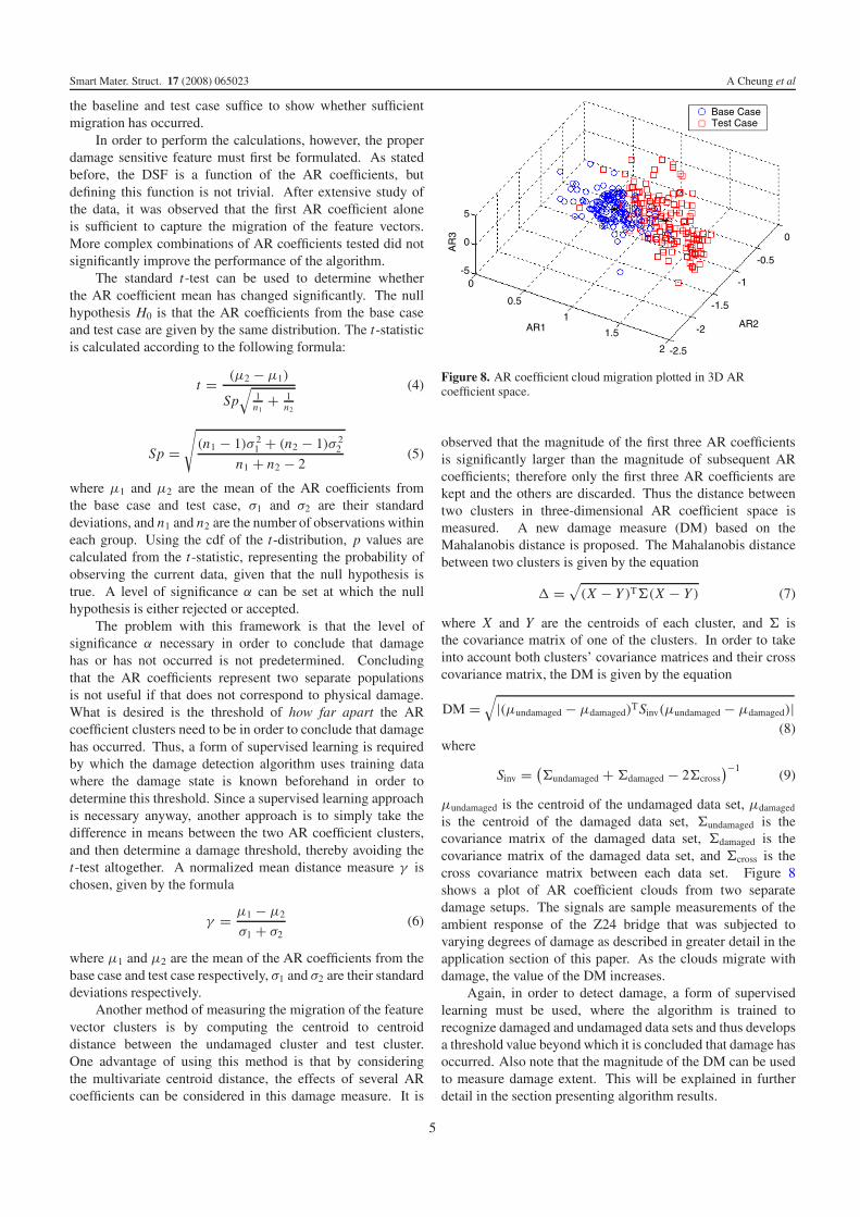
Figure 8. AR coefficient cloud migration plotted in 3D ARcoefficient space.

observed that the magnitude of the first three AR coefficientsis significantly larger than the magnitude of subsequent ARcoefficients; therefore only the first three AR coefficients arekept and the others are discarded. Thus the distance betweentwo clusters in three-dimensional AR coefficient space ismeasured. A new damage measure (DM) based on theMahalanobis distance is proposed. The Mahalanobis distancebetween two clusters is given by the equation

� =√

(X − Y )T�(X − Y ) (7)

where X and Y are the centroids of each cluster, and � isthe covariance matrix of one of the clusters. In order to takeinto account both clusters’ covariance matrices and their crosscovariance matrix, the DM is given by the equation

DM =√

|(μundamaged − μdamaged)TSinv(μundamaged − μdamaged)|(8)

where

Sinv = (�undamaged + �damaged − 2�cross

)−1(9)

μundamaged is the centroid of the undamaged data set, μdamaged

is the centroid of the damaged data set, �undamaged is thecovariance matrix of the damaged data set, �damaged is thecovariance matrix of the damaged data set, and �cross is thecross covariance matrix between each data set. Figure 8shows a plot of AR coefficient clouds from two separatedamage setups. The signals are sample measurements of theambient response of the Z24 bridge that was subjected tovarying degrees of damage as described in greater detail in theapplication section of this paper. As the clouds migrate withdamage, the value of the DM increases.

Again, in order to detect damage, a form of supervisedlearning must be used, where the algorithm is trained torecognize damaged and undamaged data sets and thus developsa threshold value beyond which it is concluded that damage hasoccurred. Also note that the magnitude of the DM can be usedto measure damage extent. This will be explained in furtherdetail in the section presenting algorithm results.

5

Smart Mater. Struct. 17 (2008) 065023 A Cheung et al

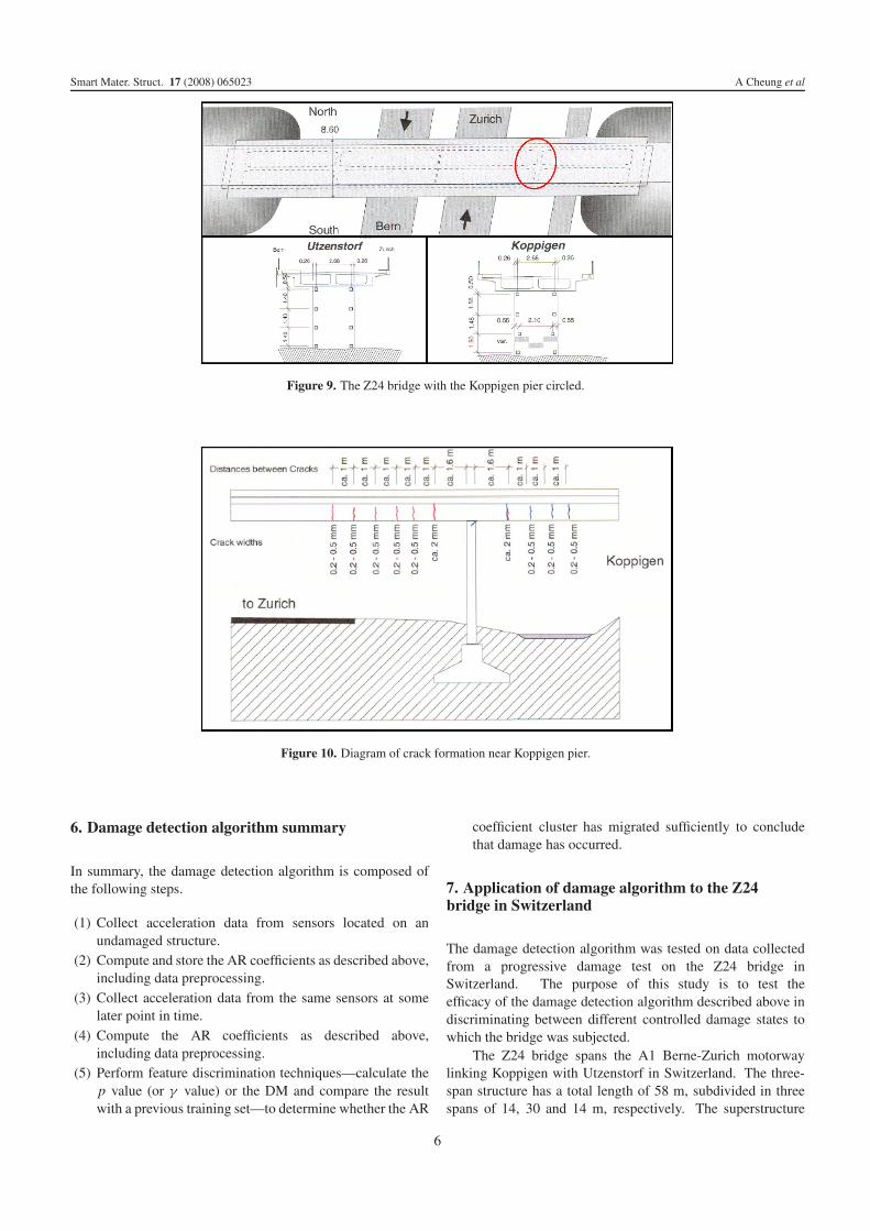
Figure 9. The Z24 bridge with the Koppigen pier circled.

Figure 10. Diagram of crack formation near Koppigen pier.

6. Damage detection algorithm summary

In summary, the damage detection algorithm is composed ofthe following steps.

(1) Collect acceleration data from sensors located on anundamaged structure.

(2) Compute and store the AR coefficients as described above,including data preprocessing.

(3) Collect acceleration data from the same sensors at somelater point in time.

(4) Compute the AR coefficients as described above,including data preprocessing.

(5) Perform feature discrimination techniques—calculate thep value (or γ value) or the DM and compare the resultwith a previous training set—to determine whether the AR

coefficient cluster has migrated sufficiently to concludethat damage has occurred.

7. Application of damage algorithm to the Z24bridge in Switzerland

The damage detection algorithm was tested on data collectedfrom a progressive damage test on the Z24 bridge inSwitzerland. The purpose of this study is to test theefficacy of the damage detection algorithm described above indiscriminating between different controlled damage states towhich the bridge was subjected.

The Z24 bridge spans the A1 Berne-Zurich motorwaylinking Koppigen with Utzenstorf in Switzerland. The three-span structure has a total length of 58 m, subdivided in threespans of 14, 30 and 14 m, respectively. The superstructure

6

Smart Mater. Struct. 17 (2008) 065023 A Cheung et al

Μ

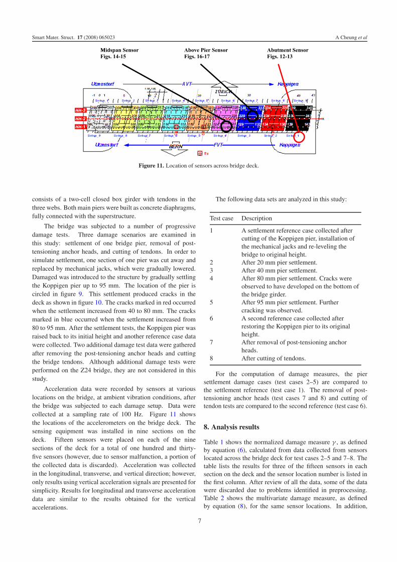
Figure 11. Location of sensors across bridge deck.

consists of a two-cell closed box girder with tendons in thethree webs. Both main piers were built as concrete diaphragms,fully connected with the superstructure.

The bridge was subjected to a number of progressivedamage tests. Three damage scenarios are examined inthis study: settlement of one bridge pier, removal of post-tensioning anchor heads, and cutting of tendons. In order tosimulate settlement, one section of one pier was cut away andreplaced by mechanical jacks, which were gradually lowered.Damaged was introduced to the structure by gradually settlingthe Koppigen pier up to 95 mm. The location of the pier iscircled in figure 9. This settlement produced cracks in thedeck as shown in figure 10. The cracks marked in red occurredwhen the settlement increased from 40 to 80 mm. The cracksmarked in blue occurred when the settlement increased from80 to 95 mm. After the settlement tests, the Koppigen pier wasraised back to its initial height and another reference case datawere collected. Two additional damage test data were gatheredafter removing the post-tensioning anchor heads and cuttingthe bridge tendons. Although additional damage tests wereperformed on the Z24 bridge, they are not considered in thisstudy.

Acceleration data were recorded by sensors at variouslocations on the bridge, at ambient vibration conditions, afterthe bridge was subjected to each damage setup. Data werecollected at a sampling rate of 100 Hz. Figure 11 showsthe locations of the accelerometers on the bridge deck. Thesensing equipment was installed in nine sections on thedeck. Fifteen sensors were placed on each of the ninesections of the deck for a total of one hundred and thirty-five sensors (however, due to sensor malfunction, a portion ofthe collected data is discarded). Acceleration was collectedin the longitudinal, transverse, and vertical direction; however,only results using vertical acceleration signals are presented forsimplicity. Results for longitudinal and transverse accelerationdata are similar to the results obtained for the verticalaccelerations.

The following data sets are analyzed in this study:

Test case Description

1 A settlement reference case collected aftercutting of the Koppigen pier, installation ofthe mechanical jacks and re-leveling thebridge to original height.

2 After 20 mm pier settlement.3 After 40 mm pier settlement.4 After 80 mm pier settlement. Cracks were

observed to have developed on the bottom ofthe bridge girder.

5 After 95 mm pier settlement. Furthercracking was observed.

6 A second reference case collected afterrestoring the Koppigen pier to its originalheight.

7 After removal of post-tensioning anchorheads.

8 After cutting of tendons.

For the computation of damage measures, the piersettlement damage cases (test cases 2–5) are compared tothe settlement reference (test case 1). The removal of post-tensioning anchor heads (test cases 7 and 8) and cutting oftendon tests are compared to the second reference (test case 6).

8. Analysis results

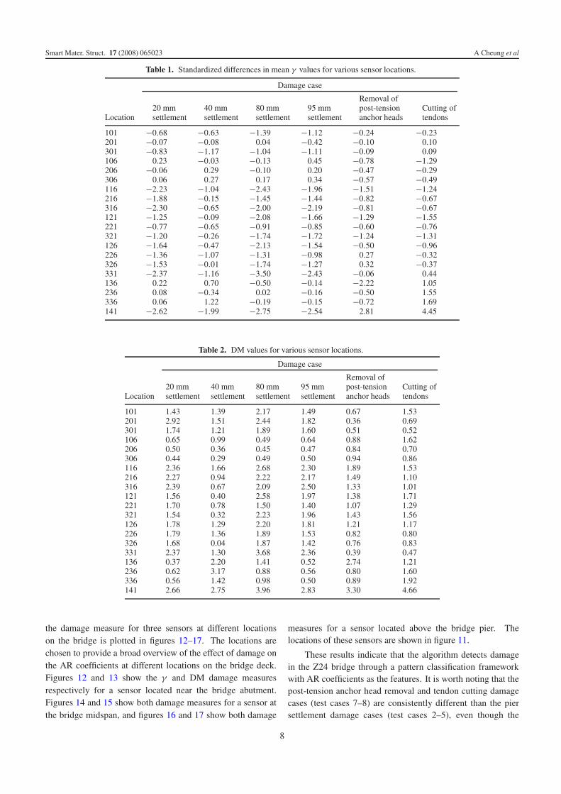
Table 1 shows the normalized damage measure γ , as definedby equation (6), calculated from data collected from sensorslocated across the bridge deck for test cases 2–5 and 7–8. Thetable lists the results for three of the fifteen sensors in eachsection on the deck and the sensor location number is listed inthe first column. After review of all the data, some of the datawere discarded due to problems identified in preprocessing.Table 2 shows the multivariate damage measure, as definedby equation (8), for the same sensor locations. In addition,

7

Smart Mater. Struct. 17 (2008) 065023 A Cheung et al

Table 1. Standardized differences in mean γ values for various sensor locations.

Damage case

Location20 mmsettlement

40 mmsettlement

80 mmsettlement

95 mmsettlement

Removal ofpost-tensionanchor heads

Cutting oftendons

101 −0.68 −0.63 −1.39 −1.12 −0.24 −0.23201 −0.07 −0.08 0.04 −0.42 −0.10 0.10301 −0.83 −1.17 −1.04 −1.11 −0.09 0.09106 0.23 −0.03 −0.13 0.45 −0.78 −1.29206 −0.06 0.29 −0.10 0.20 −0.47 −0.29306 0.06 0.27 0.17 0.34 −0.57 −0.49116 −2.23 −1.04 −2.43 −1.96 −1.51 −1.24216 −1.88 −0.15 −1.45 −1.44 −0.82 −0.67316 −2.30 −0.65 −2.00 −2.19 −0.81 −0.67121 −1.25 −0.09 −2.08 −1.66 −1.29 −1.55221 −0.77 −0.65 −0.91 −0.85 −0.60 −0.76321 −1.20 −0.26 −1.74 −1.72 −1.24 −1.31126 −1.64 −0.47 −2.13 −1.54 −0.50 −0.96226 −1.36 −1.07 −1.31 −0.98 0.27 −0.32326 −1.53 −0.01 −1.74 −1.27 0.32 −0.37331 −2.37 −1.16 −3.50 −2.43 −0.06 0.44136 0.22 0.70 −0.50 −0.14 −2.22 1.05236 0.08 −0.34 0.02 −0.16 −0.50 1.55336 0.06 1.22 −0.19 −0.15 −0.72 1.69141 −2.62 −1.99 −2.75 −2.54 2.81 4.45

Table 2. DM values for various sensor locations.

Damage case

Location20 mmsettlement

40 mmsettlement

80 mmsettlement

95 mmsettlement

Removal ofpost-tensionanchor heads

Cutting oftendons

101 1.43 1.39 2.17 1.49 0.67 1.53201 2.92 1.51 2.44 1.82 0.36 0.69301 1.74 1.21 1.89 1.60 0.51 0.52106 0.65 0.99 0.49 0.64 0.88 1.62206 0.50 0.36 0.45 0.47 0.84 0.70306 0.44 0.29 0.49 0.50 0.94 0.86116 2.36 1.66 2.68 2.30 1.89 1.53216 2.27 0.94 2.22 2.17 1.49 1.10316 2.39 0.67 2.09 2.50 1.33 1.01121 1.56 0.40 2.58 1.97 1.38 1.71221 1.70 0.78 1.50 1.40 1.07 1.29321 1.54 0.32 2.23 1.96 1.43 1.56126 1.78 1.29 2.20 1.81 1.21 1.17226 1.79 1.36 1.89 1.53 0.82 0.80326 1.68 0.04 1.87 1.42 0.76 0.83331 2.37 1.30 3.68 2.36 0.39 0.47136 0.37 2.20 1.41 0.52 2.74 1.21236 0.62 3.17 0.88 0.56 0.80 1.60336 0.56 1.42 0.98 0.50 0.89 1.92141 2.66 2.75 3.96 2.83 3.30 4.66

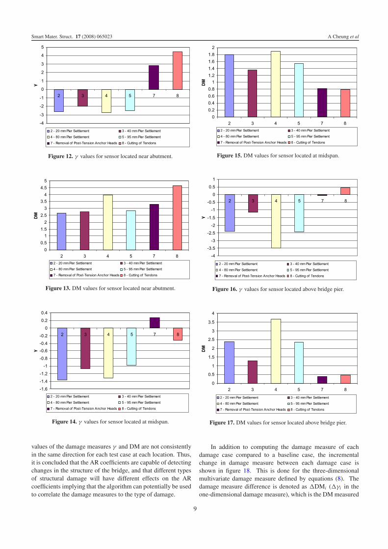
the damage measure for three sensors at different locationson the bridge is plotted in figures 12–17. The locations arechosen to provide a broad overview of the effect of damage onthe AR coefficients at different locations on the bridge deck.Figures 12 and 13 show the γ and DM damage measuresrespectively for a sensor located near the bridge abutment.Figures 14 and 15 show both damage measures for a sensor atthe bridge midspan, and figures 16 and 17 show both damage

measures for a sensor located above the bridge pier. Thelocations of these sensors are shown in figure 11.

These results indicate that the algorithm detects damagein the Z24 bridge through a pattern classification frameworkwith AR coefficients as the features. It is worth noting that thepost-tension anchor head removal and tendon cutting damagecases (test cases 7–8) are consistently different than the piersettlement damage cases (test cases 2–5), even though the

8

Smart Mater. Struct. 17 (2008) 065023 A Cheung et al

Figure 12. γ values for sensor located near abutment.

Figure 13. DM values for sensor located near abutment.

Figure 14. γ values for sensor located at midspan.

values of the damage measures γ and DM are not consistentlyin the same direction for each test case at each location. Thus,it is concluded that the AR coefficients are capable of detectingchanges in the structure of the bridge, and that different typesof structural damage will have different effects on the ARcoefficients implying that the algorithm can potentially be usedto correlate the damage measures to the type of damage.

Figure 15. DM values for sensor located at midspan.

Figure 16. γ values for sensor located above bridge pier.

Figure 17. DM values for sensor located above bridge pier.

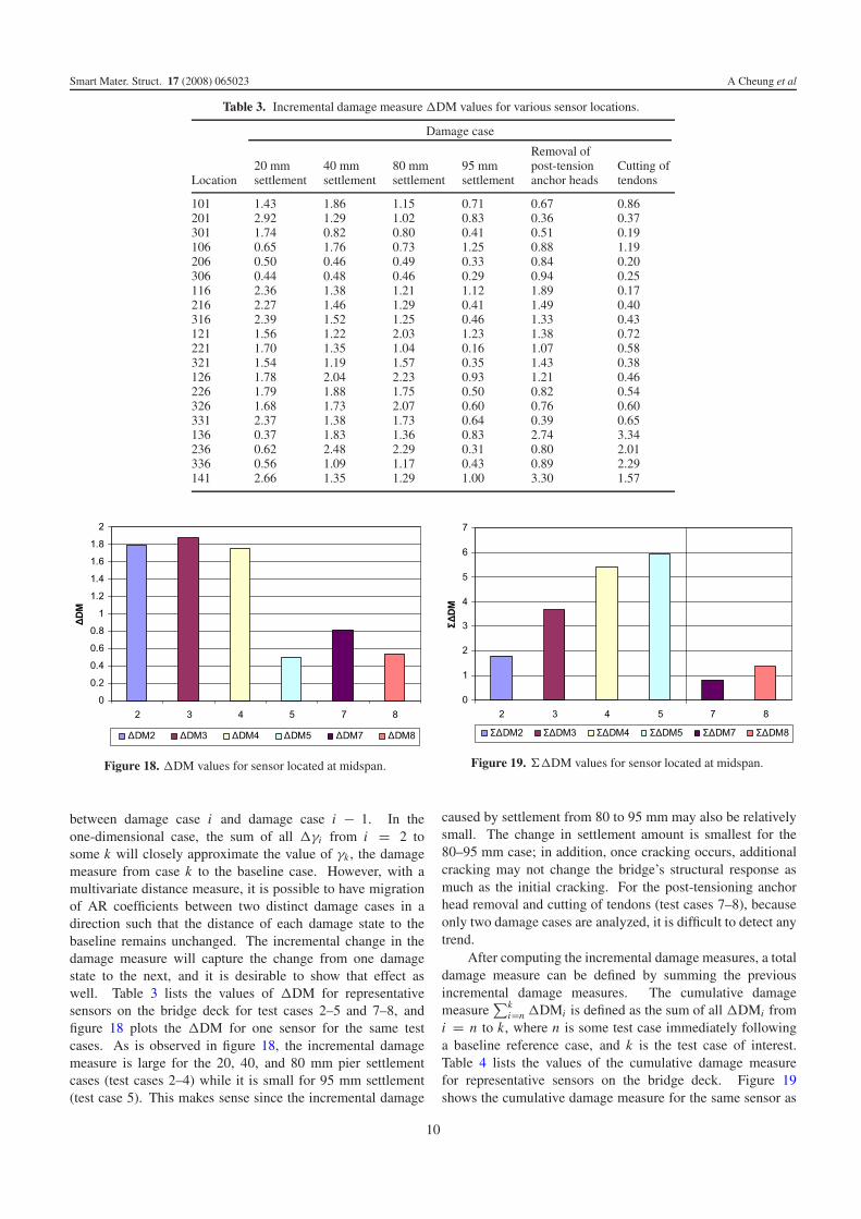
In addition to computing the damage measure of eachdamage case compared to a baseline case, the incrementalchange in damage measure between each damage case isshown in figure 18. This is done for the three-dimensionalmultivariate damage measure defined by equations (8). Thedamage measure difference is denoted as �DMi (�γi in theone-dimensional damage measure), which is the DM measured

9

Smart Mater. Struct. 17 (2008) 065023 A Cheung et al

Table 3. Incremental damage measure �DM values for various sensor locations.

Damage case

Location20 mmsettlement

40 mmsettlement

80 mmsettlement

95 mmsettlement

Removal ofpost-tensionanchor heads

Cutting oftendons

101 1.43 1.86 1.15 0.71 0.67 0.86201 2.92 1.29 1.02 0.83 0.36 0.37301 1.74 0.82 0.80 0.41 0.51 0.19106 0.65 1.76 0.73 1.25 0.88 1.19206 0.50 0.46 0.49 0.33 0.84 0.20306 0.44 0.48 0.46 0.29 0.94 0.25116 2.36 1.38 1.21 1.12 1.89 0.17216 2.27 1.46 1.29 0.41 1.49 0.40316 2.39 1.52 1.25 0.46 1.33 0.43121 1.56 1.22 2.03 1.23 1.38 0.72221 1.70 1.35 1.04 0.16 1.07 0.58321 1.54 1.19 1.57 0.35 1.43 0.38126 1.78 2.04 2.23 0.93 1.21 0.46226 1.79 1.88 1.75 0.50 0.82 0.54326 1.68 1.73 2.07 0.60 0.76 0.60331 2.37 1.38 1.73 0.64 0.39 0.65136 0.37 1.83 1.36 0.83 2.74 3.34236 0.62 2.48 2.29 0.31 0.80 2.01336 0.56 1.09 1.17 0.43 0.89 2.29141 2.66 1.35 1.29 1.00 3.30 1.57

Figure 18. �DM values for sensor located at midspan.

between damage case i and damage case i − 1. In theone-dimensional case, the sum of all �γi from i = 2 tosome k will closely approximate the value of γk , the damagemeasure from case k to the baseline case. However, with amultivariate distance measure, it is possible to have migrationof AR coefficients between two distinct damage cases in adirection such that the distance of each damage state to thebaseline remains unchanged. The incremental change in thedamage measure will capture the change from one damagestate to the next, and it is desirable to show that effect aswell. Table 3 lists the values of �DM for representativesensors on the bridge deck for test cases 2–5 and 7–8, andfigure 18 plots the �DM for one sensor for the same testcases. As is observed in figure 18, the incremental damagemeasure is large for the 20, 40, and 80 mm pier settlementcases (test cases 2–4) while it is small for 95 mm settlement(test case 5). This makes sense since the incremental damage

Figure 19. ��DM values for sensor located at midspan.

caused by settlement from 80 to 95 mm may also be relativelysmall. The change in settlement amount is smallest for the80–95 mm case; in addition, once cracking occurs, additionalcracking may not change the bridge’s structural response asmuch as the initial cracking. For the post-tensioning anchorhead removal and cutting of tendons (test cases 7–8), becauseonly two damage cases are analyzed, it is difficult to detect anytrend.

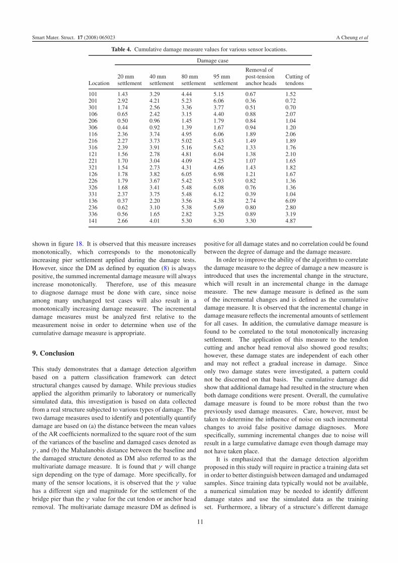
After computing the incremental damage measures, a totaldamage measure can be defined by summing the previousincremental damage measures. The cumulative damagemeasure

∑ki=n �DMi is defined as the sum of all �DMi from

i = n to k, where n is some test case immediately followinga baseline reference case, and k is the test case of interest.Table 4 lists the values of the cumulative damage measurefor representative sensors on the bridge deck. Figure 19shows the cumulative damage measure for the same sensor as

10

Smart Mater. Struct. 17 (2008) 065023 A Cheung et al

Table 4. Cumulative damage measure values for various sensor locations.

Damage case

Location20 mmsettlement

40 mmsettlement

80 mmsettlement

95 mmsettlement

Removal ofpost-tensionanchor heads

Cutting oftendons

101 1.43 3.29 4.44 5.15 0.67 1.52201 2.92 4.21 5.23 6.06 0.36 0.72301 1.74 2.56 3.36 3.77 0.51 0.70106 0.65 2.42 3.15 4.40 0.88 2.07206 0.50 0.96 1.45 1.79 0.84 1.04306 0.44 0.92 1.39 1.67 0.94 1.20116 2.36 3.74 4.95 6.06 1.89 2.06216 2.27 3.73 5.02 5.43 1.49 1.89316 2.39 3.91 5.16 5.62 1.33 1.76121 1.56 2.78 4.81 6.04 1.38 2.10221 1.70 3.04 4.09 4.25 1.07 1.65321 1.54 2.73 4.31 4.66 1.43 1.82126 1.78 3.82 6.05 6.98 1.21 1.67226 1.79 3.67 5.42 5.93 0.82 1.36326 1.68 3.41 5.48 6.08 0.76 1.36331 2.37 3.75 5.48 6.12 0.39 1.04136 0.37 2.20 3.56 4.38 2.74 6.09236 0.62 3.10 5.38 5.69 0.80 2.80336 0.56 1.65 2.82 3.25 0.89 3.19141 2.66 4.01 5.30 6.30 3.30 4.87

shown in figure 18. It is observed that this measure increasesmonotonically, which corresponds to the monotonicallyincreasing pier settlement applied during the damage tests.However, since the DM as defined by equation (8) is alwayspositive, the summed incremental damage measure will alwaysincrease monotonically. Therefore, use of this measureto diagnose damage must be done with care, since noiseamong many unchanged test cases will also result in amonotonically increasing damage measure. The incrementaldamage measures must be analyzed first relative to themeasurement noise in order to determine when use of thecumulative damage measure is appropriate.

9. Conclusion

This study demonstrates that a damage detection algorithmbased on a pattern classification framework can detectstructural changes caused by damage. While previous studiesapplied the algorithm primarily to laboratory or numericallysimulated data, this investigation is based on data collectedfrom a real structure subjected to various types of damage. Thetwo damage measures used to identify and potentially quantifydamage are based on (a) the distance between the mean valuesof the AR coefficients normalized to the square root of the sumof the variances of the baseline and damaged cases denoted asγ , and (b) the Mahalanobis distance between the baseline andthe damaged structure denoted as DM also referred to as themultivariate damage measure. It is found that γ will changesign depending on the type of damage. More specifically, formany of the sensor locations, it is observed that the γ valuehas a different sign and magnitude for the settlement of thebridge pier than the γ value for the cut tendon or anchor headremoval. The multivariate damage measure DM as defined is

positive for all damage states and no correlation could be foundbetween the degree of damage and the damage measure.

In order to improve the ability of the algorithm to correlatethe damage measure to the degree of damage a new measure isintroduced that uses the incremental change in the structure,which will result in an incremental change in the damagemeasure. The new damage measure is defined as the sumof the incremental changes and is defined as the cumulativedamage measure. It is observed that the incremental change indamage measure reflects the incremental amounts of settlementfor all cases. In addition, the cumulative damage measure isfound to be correlated to the total monotonically increasingsettlement. The application of this measure to the tendoncutting and anchor head removal also showed good results;however, these damage states are independent of each otherand may not reflect a gradual increase in damage. Sinceonly two damage states were investigated, a pattern couldnot be discerned on that basis. The cumulative damage didshow that additional damage had resulted in the structure whenboth damage conditions were present. Overall, the cumulativedamage measure is found to be more robust than the twopreviously used damage measures. Care, however, must betaken to determine the influence of noise on such incrementalchanges to avoid false positive damage diagnoses. Morespecifically, summing incremental changes due to noise willresult in a large cumulative damage even though damage maynot have taken place.

It is emphasized that the damage detection algorithmproposed in this study will require in practice a training data setin order to better distinguish between damaged and undamagedsamples. Since training data typically would not be available,a numerical simulation may be needed to identify differentdamage states and use the simulated data as the trainingset. Furthermore, a library of a structure’s different damage

11

Smart Mater. Struct. 17 (2008) 065023 A Cheung et al

patterns can be built over time for purposes of training damagedetection algorithms and these can be repeated for variousstructures.

The effects of damage to a large structure are oftencomplex with numerous locations of damage and varied typesand amounts of damage. Thus, as the complexity of thestructure increases, the damage measures are likely to identifythe damage occurrence; however, the correlation to the typeof damage will become increasingly more difficult. However,careful examination of the structure and the types of damagethat can occur locally in close proximity of a sensor can behelpful in narrowing down the many options to a manageablesize. Furthermore, use of different sensors and sensorsspecialized for specific type of damage (e.g. corrosion sensors,strain sensor, in addition to vibration sensors) can greatlyenhance our ability to more reliably predict the amount andtype of damage.

Acknowledgments

This research was partially supported by the National ScienceFoundation through an NEES Grant and by a grant fromthe National Institute from Standards and Technology, ATPContract. The authors gratefully acknowledge their support.

References

Boore D M, Stephens C D and Joyner W B 2002 Comments onbaseline correction of digital strong-motion data: examplesfrom the 1999 hector mine, California earthquake Bull. Seismol.Soc. Am. 92 1543–60

Brockwell R J and Davis R A 2003 Introduction to Time Series andForecasting 2nd edn (Berlin: Springer) p 456

Doebling S W, Farrar C R, Prime M B and Shevitz D W 1996Damage identification and health monitoring of structural andmechanical systems from changes in their vibration

characteristics: a literature review Los Alamos NationalLaboratory Report LA-13070-MS

Farrar C R and Sohn H 2000 Pattern recognition for structural healthmonitoring Workshop on Mitigation of Earthquake Disaster byAdvanced Technologies (Las Vegas, NV, Nov.–Dec.)

Farrar C R, Sohn H and Park G 2004 A statistical pattern recognitionparadigm for structural health monitoring Proc. 9th ASCE JointSpecialty Conf. on Probabilistic Mechanics and StructuralReliability (Albuquerque, NM, July)

Farrar C R, Worden K, Manson G and Park G 2005 Fundamentalaxioms of structural health monitoring Proc. 5th Int. Workshopon Structural Health Monitoring (Stanford, CA, Sept.)

Manson G, Worden K and Allman D J 2003a Experimental validationof structural health monitoring methodology II: noveltydetection on a laboratory structure J. Sound Vib. 259 345–63

Manson G, Worden K and Allman D J 2003b Experimentalvalidation of structural health monitoring methodology III:novelty detection on a laboratory structure J. Sound Vib.259 365–85

Nair K K and Kiremidjian A S 2007 Time series based structuraldamage detection algorithm using gaussian mixtures modelingASME J. Dyn. Syst. Meas. Control 129 258–93

Nair K K, Kiremidjian A S and Law K H 2006 Time series baseddamage detection and localization algorithm with application tothe ASCE benchmark structure J. Sound Vib. 291 349–68

Sohn H, Farrar C R, Hunter H F and Worden K 2001a Applying theLANL statistical pattern recognition paradigm for structuralhealth monitoring to data from a surface-effect fast patrol boatLos Alamos National Laboratory Report LA-13761-MS

Sohn H, Farrar C R, Hunter N F and Worden K 2001b Structuralhealth monitoring using statistical pattern recognitiontechniques ASME J. Dyn. Syst. Meas. Control 123 706–11(Special issue on Identification of Mechanical Systems)

Straser E G and Kiremidjian A S 1998 A modular wireless damagemonitoring system forstructures Report No. 128 John A BlumeEarthquake Engineering Center, Stanford, CA

Wenzel H 2005 personal communicationWorden K, Manson G and Allman D J 2003 Experimental validation

of structural health monitoring methodology I: novelty detectionon a laboratory structure J. Sound Vib. 259 323–43

Worden K, Manson G and Fieller N R 1999 Damage detection usingoutlier analysis J. Sound Vib. 229 647–67

12