statistical pattern recognition - sharif

Statistical Pattern Recognition

A Brief Mathematical ReviewHamid R. Rabiee

Jafar Muhammadi, Ali Jalali, Alireza Ghasemi

Spring 2013ttp://ce.sharif.edu/courses/91-92/2/ce725-1/

Sharif University of Technology, Computer Engineering Department, Pattern Recognition Course2

Agenda

Probability theory

Distribution Measures

Gaussian distribution

Central Limit Theorem

Information Measure

Distances

Linear Algebra


Probability Space

A triple of (Ω, F, P)

Ω: represents a nonempty set, whose elements are sometimes known as outcomes or states of nature (Sample Space)

F: represents a set, whose elements are called events. The events are subsets of Ω. F should be a “Borel Field”.

If a field has the property that, if the sets A1, A2,...,An,... belong to it, then so do the sets A1+A1+...+An+... and A1.A1.....An...., then the field is called a Borel field.

P: represents the probability measure.

Fact: P(Ω) = 1


Random Variables

Random variable is a “function” (“mapping”) from a set of possible

outcomes of the experiment to an interval of real (complex) numbers.

In other words:

Examples:Mapping faces of a dice to the first six natural numbers.

Mapping height of a man to the real interval (0,3] (meter or something else).

Mapping success in an exam to the discrete interval [0,20] by quantum 0.1

( ):

:X F IFX rI R

⎧⎧ →⎪⊆Ω⎪ ⎪⎪⎨ ⎨⎪ ⎪ =⊆⎪ ⎪⎩ ⎩ β


Random Variables (Cont’d)

Random VariablesDiscrete

Dice, Coin, Grade of a course, etc.

Continuous

Temperature, Humidity, Length, etc.

Random VariablesReal

Complex


Density/Distribution Functions

Probability Mass Function (PMF)Discrete random variables

Summation of impulses

The magnitude of each impulse represents the probability of occurrence of the outcome

PMF values are probabilities.

Example I:Rolling a fair dice

1 2 3 4 5 6

61

⎟⎠⎞⎜

⎝⎛βX

( )XP


Density/Distribution Functions (Cont’d)

Example II:Summation of two fair dices

Note : Summation of all probabilities should be equal to ONE. (Why?)

61

⎟⎠⎞⎜

⎝⎛βX

( )XP



Probability Density Function (PDF)Continuous random variables

The probability of occurrence of will be0 ,2 2

dx dxx x x⎛ ⎞⎟⎜ ⎟∈ − +⎜ ⎟⎜ ⎟⎜⎝ ⎠

⎟⎠⎞⎜

⎝⎛βX

( )XP

x

( )xP

( ).P x dx



Cumulative Distribution Function (CDF)Both Continuous and Discrete

Could be defined as the integration of PDF

Some CDF properties

Non-decreasing

Right Continuous

F(-infinity) = 0

F(infinity) = 1

( ) ( ) ( )

( ) ( ).

X

x

X X

CDF x F x P X x

F x f x dx−∞

= = ≤

= ∫⎟⎠⎞⎜

⎝⎛βX

( )XPDF


Famous Density Functions

Some famous masses and densitiesUniform Density

Gaussian (Normal) Density

Exponential Density

( )( )

( )2

22.1 ,. 2

x

f x e Nμσ μ σ

σ π

−−

= =

a1

⎟⎠⎞⎜

⎝⎛βX

( )XP

a

πσ 2.1

⎟⎠⎞⎜

⎝⎛βX

( )XP

μ

( ) ( ) ( )( )1 .f x U end U begina

= −

( ) ( ) . 0. .

0 0

xx e x

f x e U xx

λλ λλ

−−

⎧⎪ ≥⎪= = ⎨⎪ <⎪⎩


Joint/Conditional Distributions

Joint Probability Functions

Example I

In a rolling fair dice experiment represent the outcome as a 3-bit digital number “xyz”.

( ),

1 0; 061 0; 131, 1; 031 1; 160 . .

X Y

x y

x y

f x y x y

x y

OW

⎧⎪ = =⎪⎪⎪⎪⎪ = =⎪⎪⎪⎪⎪⎪= = =⎨⎪⎪⎪⎪ = =⎪⎪⎪⎪⎪⎪⎪⎪⎩

1 001

4 1005 101

xyz

2 0103 011

6 110

→→→→→→

( ) ( )

( )

,

,

,

,

X Y

yx

X Y

F x y P X x and Y y

f x y dydx−∞−∞

= ≤ ≤

= ∫ ∫


Joint/Conditional Distributions (Cont’d)

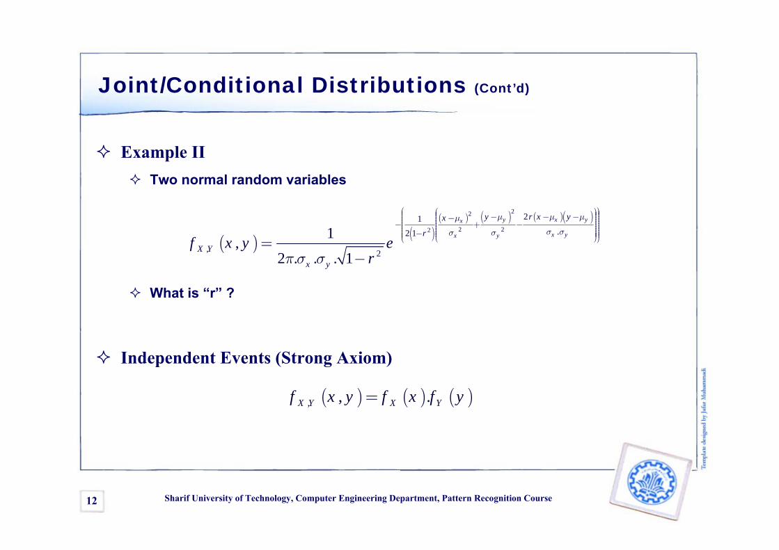
Example IITwo normal random variables

What is “r” ?

Independent Events (Strong Axiom)

( ) ( )( ) ( ) ( )( )22

2 22

21.2 1

, 2

1,2 . . . 1

y x yx

x yx y

y r x yx

r

X Y

x y

f x y er

μ μ μμσ σσ σ

π σ σ

⎛ ⎞⎛ ⎞⎟⎟⎜ ⎜ ⎟⎟− − −⎜ ⎜ − ⎟⎟⎜ ⎜ ⎟⎟⎜ ⎟⎜ ⎟− + −⎜ ⎟⎜ ⎟⎟⎜ ⎟⎜ ⎟⎟⎜ ⎜ ⎟⎟⎜ − ⎜ ⎟⎟⎟⎜⎜ ⎟⎜ ⎝ ⎠⎝ ⎠=−

( ) ( ) ( ), , .X Y X Yf x y f x f y=



Obtaining one variable densitydensity functions

DistributionDistribution functions can be obtained just from the density functions. (How?)

( ) ( )

( ) ( )

,

,

,

,

X X Y

Y X Y

f x f x y dy

f y f x y dx

∞

−∞∞

−∞

=

=

∫

∫



Conditional Density Function

Probability of occurrence of an event if another event is observed (we know what “Y” is).

Bayes’ Rule

( ) ( )( )

, ,X YX Y

Y

f x yf x y

f y=

( )( ) ( )

( ) ( )

.

.

XY XX Y

XY X

f y x f xf x y

f y x f x dx∞

−∞

=

∫



Example IRolling a fair dice

X : the outcome is an even number

Y : the outcome is a prime number

Example IIJoint normal (Gaussian) random variables

( ) ( )( )

1, 161 3

2

P X YP X Y

P Y= = =

( ) ( )2

21

2 1

2

12 . . 1

yx

x y

yx rr

X Y

x

f x y er

μμσ σ

π σ

⎛ ⎞⎟⎜ ⎛ ⎞ ⎟− ⎟⎜ ⎜ − ⎟⎟⎜ ⎜ ⎟⎟⎜ ⎜ ⎟− − × ⎟⎜ ⎟⎜ ⎟ ⎟⎜ ⎜ ⎟ ⎟⎟⎜ ⎟⎜⎜ ⎟− ⎝ ⎠⎜ ⎟⎜⎝ ⎠=−



Conditional Distribution Function

Note that “y” is a constant during the integration.

( ) ( )

( )

( )

( )

,

,

,

,

X Y

x

X Y

x

X Y

X Y

F x y P X x while Y y

f x y dx

f t y dt

f t y dt

−∞

−∞∞

−∞

= ≤ =

=

=

∫

∫

∫



Independent Random Variables

( ) ( )( )( ) ( )( )

( )

, ,

.

X YX Y

Y

X Y

Y

X

f x yf x y

f y

f x f yf y

f x

=

=

=


Distribution Measures

Most basic type of descriptor for spatial distributions, include:Mean Value

Variance & Standard Deviation

Covariance

Correlation Coefficient

Moments


Expected Value

Expected value ( population mean value)

Properties of Expected Value

The expected value of a constant is the constant itself. E[b]= b

If a and b are constants, then E[aX+ b]= a E[X]+ b

If X and Y are independent RVs, then E[XY]= E[X ]* E[Y]

If X is RV with PDF f(X), g(X) is any function of X, then,

if X is discrete

if X is continuous

E[ ( )] ( ) ( )g X xf x xf x dx∞

−∞= =∑ ∫

E[ ( )] ( ) ( )g X g X f x=∑

[ ( )] ( ) ( )E g X g X f x dx∞

−∞= ∫


Variance & Standard Deviation

Let X be a RV with E(X)=u, the distribution, or spread, of the X values around the

expected value can be measured by the variance ( is the standard deviation of X).

The Variance Properties

The variance of a constant is zero.

If a and b are constants, then

If X and Y are independent RVs, then

xδ

2 2

2

2 2 2 2

var( ) ( )

( ) ( )

( ) ( ) [ ( )]

x

x

X E X

X f x

E X E X E X

δ μμ

μ

= = −= −

= − = −

∑

2var( ) var( )aX b a X+ =

var( ) var( ) var( )X Y X Y+ = +var( ) var( ) var( )X Y X Y− = +


Covariance

Covariance of two RVs, X and Y: Measurement of the nature of the association

between the two.

Properties of Covariance:If X, Y are two independent RVs, then

If a, b, c and d are constants, then

If X is a RV, then

Covariance ValueCov(X,Y) is positively big = Positively strong relationship between the two.

Cov(X,Y) is negatively big = Negatively strong relationship between the two.

Cov(X,Y)=0 = No relationship between the two.

( , ) [( )( )] ( )x y x yCov X Y E X Y E XYμ μ μ μ= − − = −

( ) ( ) ( ) 0x y x yCov E XY E x E yμ μ μ μ= − = − =

( , ) cov( , )Cov a bX c dY bd X Y+ + =2 2( ) ( )xCov E X Var Xμ= − =


Variance of Correlated Variables

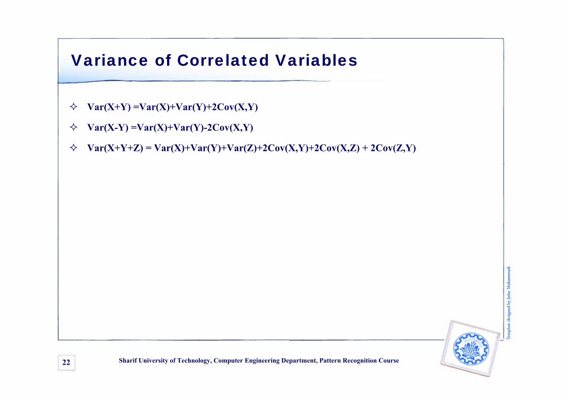
Var(X+Y) =Var(X)+Var(Y)+2Cov(X,Y)

Var(X-Y) =Var(X)+Var(Y)-2Cov(X,Y)

Var(X+Y+Z) = Var(X)+Var(Y)+Var(Z)+2Cov(X,Y)+2Cov(X,Z) + 2Cov(Z,Y)


Covariance Matrices

If X is a n-Dim RV, then the covariance defined as:

whose ijth element σij is the covariance of xi and xj:

then

[( )( ) ]tx xE∑ = − −x μ x μ

( , ) [( )( )], , 1, , .i j ij i i j jCov x x E x x i j dσ μ μ= = − − = …

211 12 1 1 12 1

221 22 2 21 2 2

21 2 1 2

d d

d d

d d dd d d d

σ σ σ σ σ σσ σ σ σ σ σ

σ σ σ σ σ σ

⎡ ⎤⎡ ⎤⎢ ⎥⎢ ⎥⎢ ⎥⎢ ⎥∑ = =⎢ ⎥⎢ ⎥⎢ ⎥⎢ ⎥⎢ ⎥⎣ ⎦ ⎣ ⎦


Covariance Matrices (cont’d)

Properties of Covariance Matrix:

If the variables are statistically independent, the covariances are zero, and the covariance matrix is diagonal.

noting that the determinant of Σ is just the product of the variances, then we can write

This is the general form of a multivariate normal density function, where the covariance matrix is no longer required to be diagonal.

2 21 1

2 212 2

2 2

0 0 1/ 0 00 0 0 1/ 0

0 0 0 0 1/d d

σ σσ σ

σ σ

−

⎡ ⎤ ⎡ ⎤⎢ ⎥ ⎢ ⎥⎢ ⎥ ⎢ ⎥∑ = ⇒ ∑ =⎢ ⎥ ⎢ ⎥⎢ ⎥ ⎢ ⎥⎢ ⎥ ⎢ ⎥⎣ ⎦ ⎣ ⎦

21( ) ( )tx μ

σ−⎛ ⎞−

⇒ = − ∑ −⎜ ⎟⎝ ⎠

x μ x μ

11 ( ) ( )2

1/ 2/ 2

1( )(2 )

t

dp x e

π

−− − ∑ −=

∑

x μ x μ


Correlation Coefficient

Correlation: Knowing about a random variable “X”, how much

information will we gain about the other random variable “Y” ?

The population correlation coefficient is defined as

The Correlation Coefficient is a measure of linear association between two

variables and lies between -1 and +1

-1 indicating perfect negative association

+1 indicating perfect positive association

cov( , )

x y

X Yρδ δ

=


Moments

Momentsnth order moment of a RV X is the expected value of Xn:

Normalized form (Central Moment)

Mean is first moment

Variance is second moment added by the square of the mean.

( )( )nn XM E X μ= −

( )nnM E X=


Moments (cont’d)

Third MomentMeasure of asymmetry

Often referred to as skewness

Fourth Moment

Measure of flatness

Often referred to as Kurtosis

3( ) ( )s x f x dxμ∞

−∞

= −∫

If symmetric s= 0

4( ) ( )k x f x dxμ∞

−∞

= −∫

small kurtosis large kurtosis


Sample Measures

Sample: a random selection of items from a lot or population in order to evaluate

the characteristics of the lot or population

Sample Mean:

Sample Variance:

Sample Covariance:

Sample Correlation:

3th center moment

4th center moment

1

nii

x x=

= ∑2

21

( )1

nx i

X XSn=

−=

−∑( )( )

( , )1

i iX X Y YCov X Y

n− −

=−

∑

( )( ) /( 1)i i

x y

X X Y Y nCorr

S S− − −

= ∑3

1

( )1

n

i

X Xn=

−−∑

4

1

( )1

n

i

X Xn=

−−∑


Gaussian distribution

( )( )

( )2

22.1 ,. 2

x

f x e Nμσ μ σ

σ π

−−

= =


More on Gaussian Distribution

The Gaussian Distribution Function Sometimes called “Normal” or “bell shaped”

Perhaps the most used distribution in all of science

Is fully defined by 2 parameters

95% of area is within 2σ

Normal distributions range from minus infinity to plus infinity

-4 -3 -2 -1 1 2 3 4

0.1

0.2

0.3

0.4

Gaussian with μ=0 and σ=1

( )( )

( )2

22.1 ,. 2

x

f x e Nμσ μ σ

σ π

−−

= =πσ 2.

1

⎟⎠⎞⎜

⎝⎛βX

( )XP

μ


More on Gaussian Distribution (Cont’d)

Normal Distributions with the Same Variance but Different Means

Normal Distributions with the Same Means but Different Variances


More on Gaussian Distribution

Standard Normal Distribution

A normal distribution whose mean is zero and standard deviation is one is called the

standard normal distribution.

any normal distribution can be converted to a standard normal distribution with simple algebra. This makes calculations much easier.

2121( )

2

xf x e

π−

=

XZ μσ−=


Gaussian Function Properties

Gaussian has relatively simple analytical properties

It is closed under linear transformation

The Fourier transform of a Gaussian is Gaussian

The product of two Gaussians is also Gaussian

All marginal and conditional densities of a Gaussian are Gaussian

Diagonalization of covariance matrix rotated variables are independent

Gaussian distribution is infinitely divisible


Why Gaussian Distribution?

Central Limit TheoremWill be discussed later

Binomial distribution

The last row of Pascal's triangle (the binomial distribution) approaches a sampled Gaussian function as the number of rows increases.

Some distribution cab be estimated by Normal distribution for sufficiently

large parameter valuesBinomial distribution

Poisson distribution


Covariance Matrix Properties

[ ]E Xμ=

( )T TE XX μμΣ = −

var( ) var( ) TAX a A X A+ =cov( , ) cov( , )TX Y Y X=

1 2 1 2cov( , ) cov( , ) cov( , )X X Y X Y X Y+ = +

var( ) var( ) var( ) cov( , ) cov( , )X Y X Y X Y Y X+ = + + +

cov( , ) cov( , ) TAX BY A X Y B=

[( [ ])( [ ]) ]TE X E X X E XΣ = − −



Why is The Gaussian PDF is so applicable? Central Limit Theorem

Illustrating CLT

a) 5000 Random Numbers

b) 5000 Pairs (r1+r2) of Random Numbers

c) 5000 Triplets (r1+r2+r3) of Random Numbers

d) 5000 12-plets (r1+r2+…+r12) of Random Numbers


Central Limit Theorem says that

we can use the standard normal approximation of the sampling distribution

regardless of our data. We don’t need to know the underlying probability distribution of the data to make use of sample statistics.

This only holds in samples which are large enough to use the CLT’s “large sample properties.” So, how large is large enough?

Some books will tell you 30 is large enough.

Note: The CLT does not say: “in large samples the data is distributed normally.”



Two Normal-like distributions

T-Student Distribution

Chi-Squared Distribution

22 2 ( / 2) 1 / 2/ 2

1 1( ) ( )( / 2) 2

vvf e

vχχ χ − −=

Γ

( ) ( 1) / 221 / 2( ) 1

( / 2)

vv tf tvv vπ

− +⎡ ⎤ ⎡ ⎤Γ +⎢ ⎥⎣ ⎦ ⎢ ⎥= +⎢ ⎥Γ ⎣ ⎦


Information Measure Criteria

Information gainLet pi be the probability that a sample in D belongs to class Ci (estimated by |Ci|/|D|)

Expected information (entropy) needed to classify a sample in D:

Information needed to classify a sample in D, after using A to split D into v partitions :

Information gained by attribute A

m

i 2 ii 1

Info(D) p log (p )=

=−∑

vj

A jj 1

|D |Info (D) Info(D )

|D|== ×∑

AGain(A) Info(D) Info (D)= −



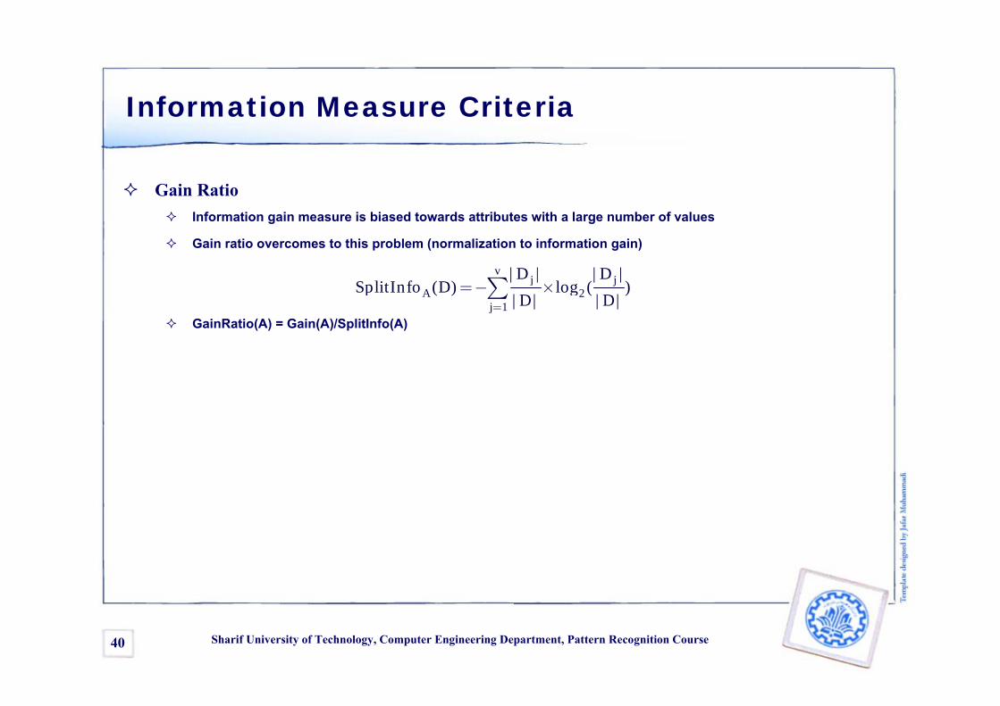
Gain RatioInformation gain measure is biased towards attributes with a large number of values

Gain ratio overcomes to this problem (normalization to information gain)

GainRatio(A) = Gain(A)/SplitInfo(A)

vj j

A 2j 1

|D | |D |SplitInfo (D) log ( )

|D| |D|==− ×∑



Gini indexIf a data set D contains examples from n classes, gini index, gini(D) is defined as

If a dataset D is split on A into two subsets D1 and D2, the gini index gini(D) is defined as

Reduction in Impurity:

The attribute provides the largest reduction in impurity is the best

n 2gini(D) 1 p jj 1

= − ∑=

1 21 2A

|D | |D |(D) gini( ) gini( )gini D D|D| |D|

= +

Agini(A) gini(D) gini (D)Δ = −



ComparisonInformation gain:

biased towards multivalued attributes

Gain ratio:

tends to prefer unbalanced splits in which one partition is much smaller than the others

Gini index:

biased to multivalued attributes

has difficulty when # of classes is large

Tends to favor tests that result in equal-sized partitions and purity in both partitions


Distances

Each clustering problem is based on some kind of “distance” between points.An Euclidean space has some number of real-valued dimensions and some data points.

A Euclidean distance is based on the locations of points in such a space.

A Non-Euclidean distance is based on properties of points, but not their “location” in a

space.

Distance MatricesOnce a distance measure is defined, we can calculate the distance between objects.

These objects could be individual observations, groups of observations (samples) or populations of observations.

For N objects, we then have a symmetric distance matrix D whose elements are the distances between objects i and j.


Axioms of a Distance Measure

d is a distance measure if it is a function from pairs of points to reals such

that:1. d(x,y) > 0.

2. d(x,y) = 0 iff x = y.

3. d(x,y) = d(y,x).

4. d(x,y) < d(x,z) + d(z,y) (triangle inequality ).

For the purpose of clustering, sometimes the distance (similarity) is not

required to be a metricNo Triangle Inequality

No Symmetry


Distance Measures

Minkowski Distance The Minkowski distance of order p between two points is defined as:

L2 Norm (Euclidean Distance): p=2

L1 Norm (Manhattan Distance): p=1

L∞ Norm: p= ∞

1

1

n ppi i

kx y

=

⎛ ⎞−⎜ ⎟⎝ ⎠∑


Euclidean Distance (L1, L∞ Norm)

L1 Norm: sum of the differences in each dimension.Manhattan distance = distance if you had to travel along coordinates only.

L∞ norm : d(x,y) = the maximum of the differences between x and y in

any dimension.

x = (5,5)

y = (9,8)

L2-norm:

dist(x,y) = √(42+32) =5

L1-norm:dist(x,y) = 4+3 = 7

4

35

L∞ -norm:dist(x,y) = Max(4, 3) = 4


Mahalanobis Distance

Distances are computed based on means, variances and covariances for

each of g samples (populations) based on p variables.

Mahalanobis distance “weights” the contribution of each pair of variables

by the inverse of their covariance.

are samples means.

is the Covariance between samples.

2 1( ) ( )Tij i j i jD μ μ μ μ−= − Σ −

,i jμ μ

Σ


KL Divergence

Defined between two probability distributions

Measures the expected number of extra bits in case of using Q rather than P

Can be used as a distance measure when feature vectors form distributions

However, it is not a true metricTriangle equality and symmetry do not hold

Symmetric variants have been proposed

KLi

log P(i)D (P ||Q) P(i)

log Q(i)=∑


Linear Algebra – Review on Vectors

N-dimensional vectors

Unit Vector:Any vector with magnitude equal to one

Inner product: Given two vectors v=(x1,x2,x3,…,xn) and w=(y1,y2,y3,…,yn)

[ ]1

T

1 n

n

x

v x x

x

⎡ ⎤⎢ ⎥⎢ ⎥= =⎢ ⎥⎢ ⎥⎢ ⎥⎣ ⎦

T||v|| v v=

1 1 2 2 n nv .w x y x y x y= + + +


More About Vectors

Geometrically-based definition of dot product

Orthonormal VectorsA set of vectors x1,x2,…,xn is called orthonormal if

Any basis (x1, x2, . . . , xn) can be converted to an orthonormal basis (o1, o2, . . . , on) using the Gram-Schmidt orthogonalization procedure.

v.w || v ||.||w ||.cos( ) ( is the smallest angle between v and w)= θ θ

j

Ti

1 if i jx x

0 if i j

⎧ =⎪⎪=⎨⎪ ≠⎪⎩


Vector Space

Given a set of objects W we see that W is a vector space if

In general, F is the set of real numbers and W is a set of vectors

A linear combination of vectors v1,…vk is defined as

c1,…ck are scalars

Spanning

We say that the set of vectors S=(v1,…vk ) span a space W if every vector in W can be written as a linear combination of the vectors in S

u v W for all F and u,v Wλ + ∈ λ∈ ∈

1 1 2 2 k kv c v c v c v= + +


Linear Independence

A set of vectors v1,…,vk is linearly independent if:c1v1 + c2v2 + . . . + ck vk = 0 implies c1 = c2 = . . . = ck = 0

Geometric interpretation of linear independence

In R2 or R3, two vectors are linearly independent if they do not lie on the same line.

In R3, there vectors are linearly independent if they do not lie in the same plane.


Basis

A set of vectors S=(v1, ..., vk) is said to be a basis for a vector space W if(1) the vjs are linearly independent

(2) S spans W

Warning: The vectors forming a basis are not necessarily orthogonal !

Theorem I: If V is an n-dimensional vector space, and if S is a set in V with

exactly n vectors, then S is a basis for V if either S spans V or S is linearly

independent.


Matrices

Matrix transpose

(AB)T=BTAT

Symmetric matrix : AT=A

11 12 1n 11 21 m1

21 22 2n 12 22 m2T

m1 mn 1n 2n mn

a a . . a a a . . a

a a . . a a a . . a

A , A. . . . . . . . . .

. . . . . . . .

a . . . a a a . . a

⎡ ⎤ ⎡ ⎤⎢ ⎥ ⎢ ⎥⎢ ⎥ ⎢ ⎥⎢ ⎥ ⎢ ⎥⎢ ⎥ ⎢ ⎥= =⎢ ⎥ ⎢ ⎥⎢ ⎥ ⎢ ⎥⎢ ⎥ ⎢ ⎥⎢ ⎥ ⎢ ⎥⎢ ⎥ ⎢ ⎥⎣ ⎦ ⎣ ⎦


Linear Algebra – Determinant

Determinant

det(AB)= det(A)det(B)

Eigenvectors and Eigenvalues

Characteristic equation

Determinant & Eigen values

ni j

ij n n ij ij ij ijj 1

A [a ] ; det(A) a A ; i 1,....n; A ( 1) det(M )+×

== = = = −∑

j j j jAe e , j 1,...,n; ||e || 1=λ = =

ndet[A I ] 0−λ =

n

jj 1

det[A]=

= λ∏


Matrix Inverse

Matrix inverse (matrix must be square)The inverse A-1 of matrix A has the property: AA-1=A-1A=I

A-1 exists only if det(A)≠0

Singular: the inverse of A does not exist

ill-conditioned: A is nonsingular but close to being singular

Some properties of the inverse:det(A-1) =det(A)-1

(AB)-1=B-1A-1

(AT )-1 = (A-1)T


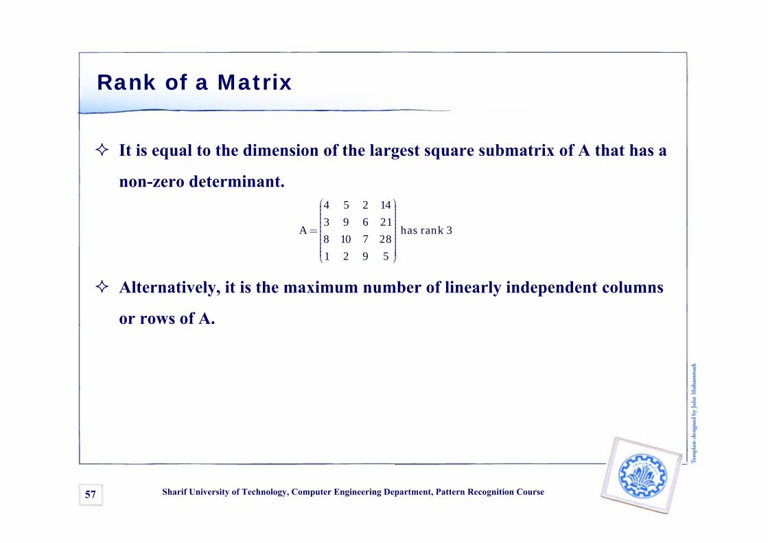
Rank of a Matrix

It is equal to the dimension of the largest square submatrix of A that has a

non-zero determinant.

Alternatively, it is the maximum number of linearly independent columns

or rows of A.

4 5 2 14

3 9 6 21A has rank 3

8 10 7 28

1 2 9 5

⎛ ⎞⎟⎜ ⎟⎜ ⎟⎜ ⎟⎜ ⎟⎜ ⎟⎜ ⎟= ⎟⎜ ⎟⎜ ⎟⎜ ⎟⎜ ⎟⎜ ⎟⎟⎜⎝ ⎠


Matrix Properties Based on Rank

If A is m×n, rank(A) ≤ min m, n

If A is n×n, rank(A) = n iff A is nonsingular (i.e., invertible).

If A is n×n, rank(A) = n iff det(A)≠0 (full rank).

If A is n×n, rank(A) < n iff A is singular


Any Question

End of Lecture 2

Thank you!Spring 2013

http://ce.sharif.edu/courses/91-92/2/ce725-1/

statistical pattern recognition - sharif

Documents