recognition template matching o chamfer matching statistical pattern recognition (spr) robust...
TRANSCRIPT
RecognitionTemplate Matching
o Chamfer MatchingStatistical Pattern Recognition (SPR)Robust object recognition using a cascade of Haar classifiers (Haar)Performance
RecognitionBased on A Practical Introduction to Computer Vision with
OpenCV by Kenneth Dawson-Howe © Wiley & Sons Inc. 2014 Slide 1

Template Matching - Topics Applications Matching criteria Use of Fourier space Use of chamfering Control strategies
RecognitionBased on A Practical Introduction to Computer Vision with
OpenCV by Kenneth Dawson-Howe © Wiley & Sons Inc. 2014 Slide 2
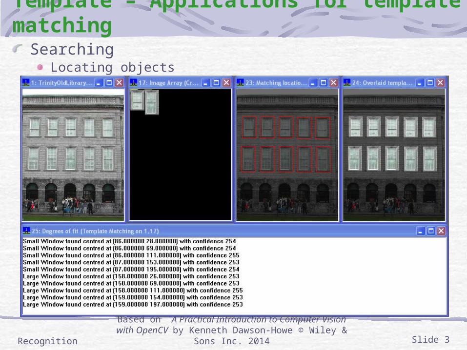
Template – Applications for template matching Searching
Locating objects
RecognitionBased on A Practical Introduction to Computer Vision with
OpenCV by Kenneth Dawson-Howe © Wiley & Sons Inc. 2014 Slide 3
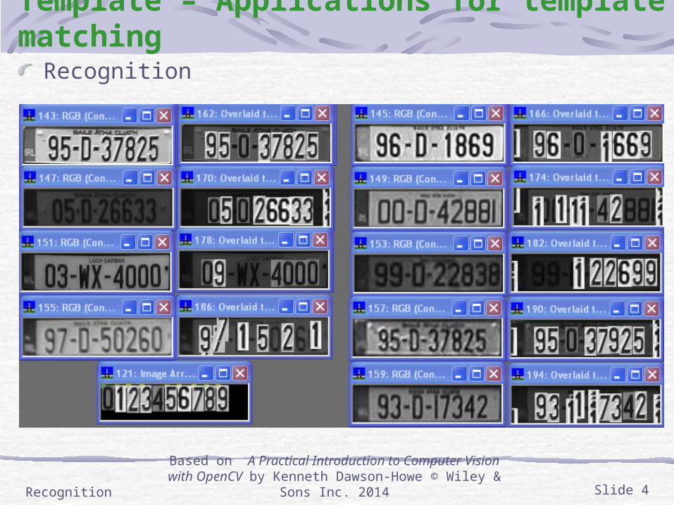
Template – Applications for template matching Recognition
RecognitionBased on A Practical Introduction to Computer Vision with
OpenCV by Kenneth Dawson-Howe © Wiley & Sons Inc. 2014 Slide 4
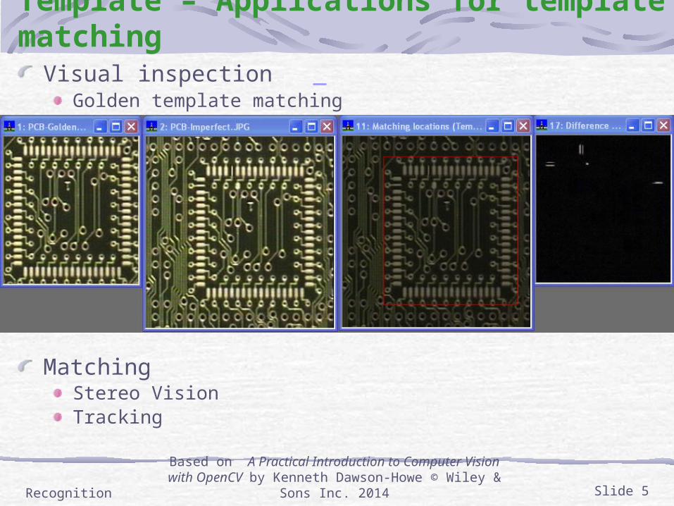
Template – Applications for template matching Visual inspection
Golden template matching
MatchingStereo VisionTracking
RecognitionBased on A Practical Introduction to Computer Vision with
OpenCV by Kenneth Dawson-Howe © Wiley & Sons Inc. 2014 Slide 5
Template – Matching AlgorithmBasic Algorithm
Inputs – Image & ObjectFor every possible position of the object in the image
Evaluate a match criterionSearch for local maxima of the match criterion above some threshold
Problems‘Every possible position’?‘Match criterion’ ‘Local maxima above some threshold’
RecognitionBased on A Practical Introduction to Computer Vision with
OpenCV by Kenneth Dawson-Howe © Wiley & Sons Inc. 2014 Slide 6
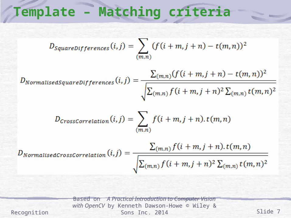
Template – Matching criteria
RecognitionBased on A Practical Introduction to Computer Vision with
OpenCV by Kenneth Dawson-Howe © Wiley & Sons Inc. 2014 Slide 7
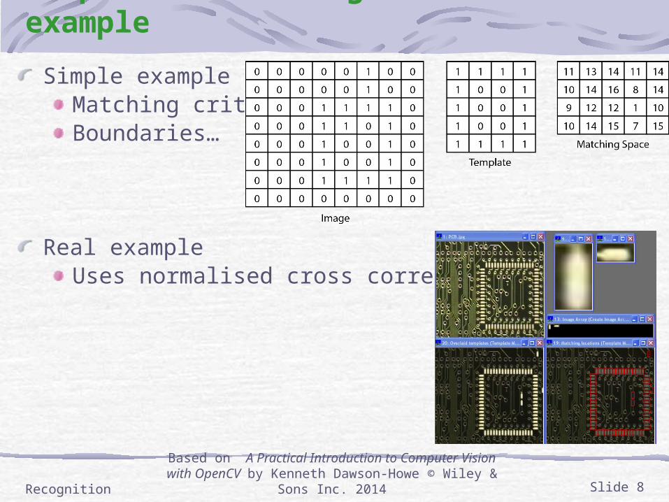
Template – Matching criteria example
Simple exampleMatching criteriaBoundaries…
Real example Uses normalised cross correlation.
RecognitionBased on A Practical Introduction to Computer Vision with
OpenCV by Kenneth Dawson-Howe © Wiley & Sons Inc. 2014 Slide 8
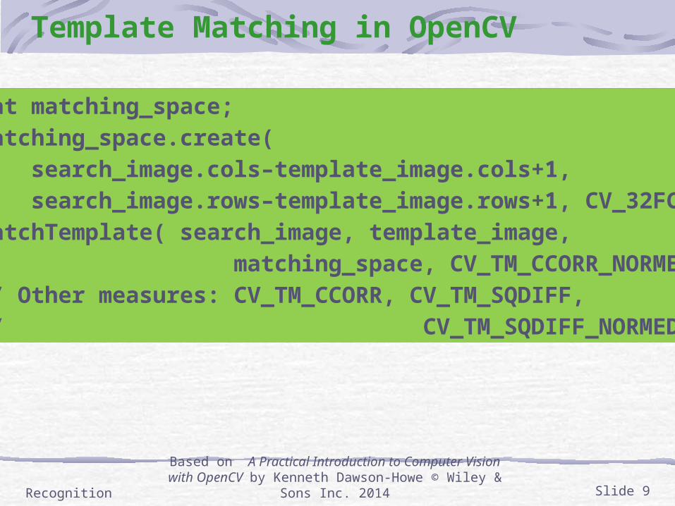
Template Matching in OpenCV
RecognitionBased on A Practical Introduction to Computer Vision with
OpenCV by Kenneth Dawson-Howe © Wiley & Sons Inc. 2014 Slide 9
Mat matching_space;
matching_space.create(
search_image.cols–template_image.cols+1,
search_image.rows–template_image.rows+1, CV_32FC1 );
matchTemplate( search_image, template_image,
matching_space, CV_TM_CCORR_NORMED );
// Other measures: CV_TM_CCORR, CV_TM_SQDIFF,
// CV_TM_SQDIFF_NORMED
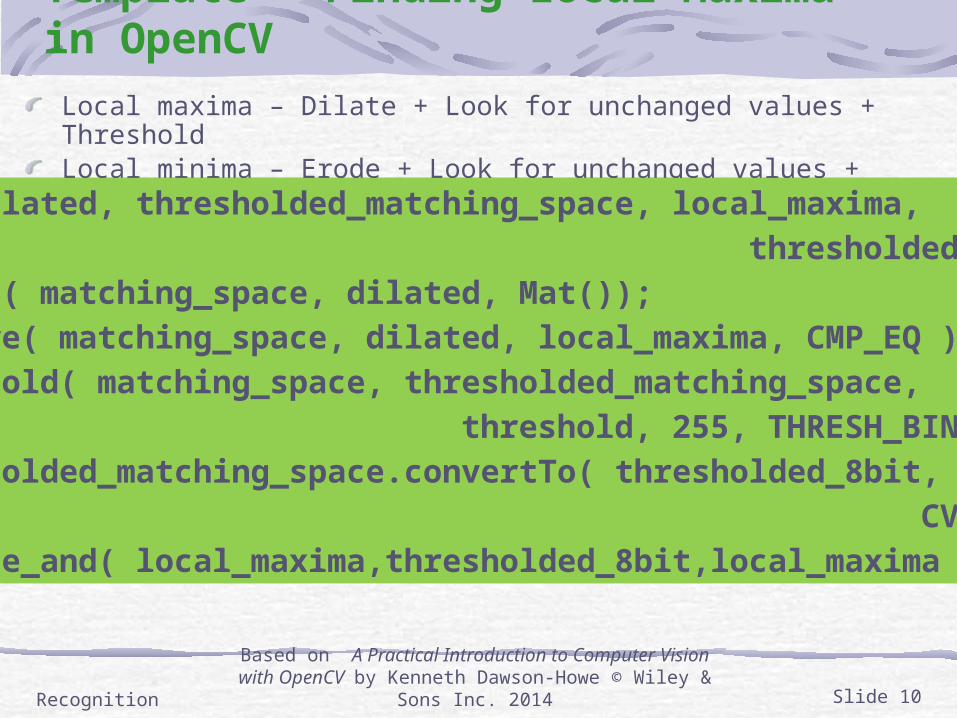
Template – Finding Local Maxima in OpenCVLocal maxima – Dilate + Look for unchanged values + ThresholdLocal minima – Erode + Look for unchanged values + Threshold
RecognitionBased on A Practical Introduction to Computer Vision with
OpenCV by Kenneth Dawson-Howe © Wiley & Sons Inc. 2014 Slide 10
Mat dilated, thresholded_matching_space, local_maxima,
thresholded_8bit;
dilate( matching_space, dilated, Mat());
compare( matching_space, dilated, local_maxima, CMP_EQ );
threshold( matching_space, thresholded_matching_space,
threshold, 255, THRESH_BINARY );
thresholded_matching_space.convertTo( thresholded_8bit,
CV_8U );
bitwise_and( local_maxima,thresholded_8bit,local_maxima );
Template – Control Strategies for MatchingGoal: Localise close copies
Size, orientationGeometric distortion
Use an image hierarchyLow resolution firstLimit higher resolution search
Search higher probability locations firstKnown / learnt likelihoodFrom lower resolution
RecognitionBased on A Practical Introduction to Computer Vision with
OpenCV by Kenneth Dawson-Howe © Wiley & Sons Inc. 2014 Slide 11
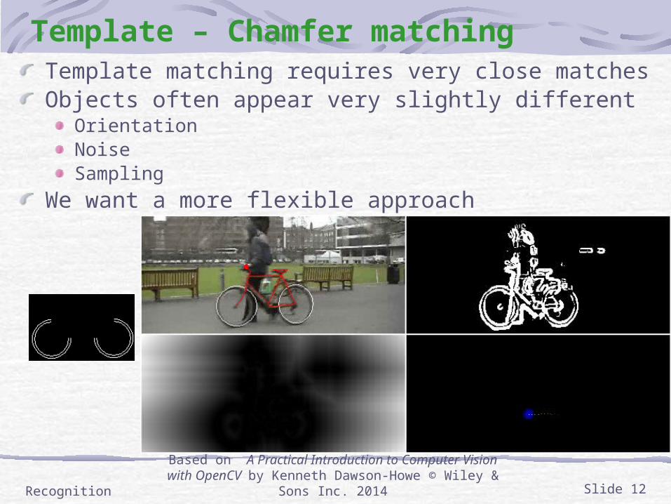
Template – Chamfer matchingTemplate matching requires very close matchesObjects often appear very slightly different
OrientationNoiseSampling
We want a more flexible approach
RecognitionBased on A Practical Introduction to Computer Vision with
OpenCV by Kenneth Dawson-Howe © Wiley & Sons Inc. 2014 Slide 12
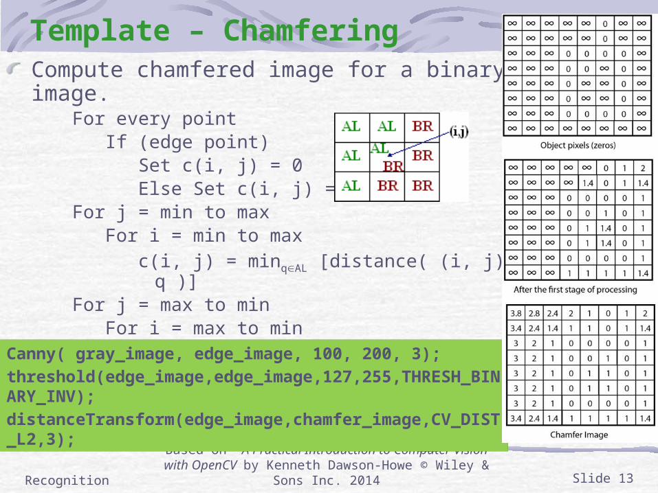
Template – ChamferingCompute chamfered image for a binary edge image.
For every pointIf (edge point)
Set c(i, j) = 0Else Set c(i, j) = ∞
For j = min to maxFor i = min to max
c(i, j) = minqAL [distance( (i, j), q ) + f( q )]For j = max to min
For i = max to minc(i, j) = minqBR [distance( (i, j), q ) + f( q )]
RecognitionBased on A Practical Introduction to Computer Vision with
OpenCV by Kenneth Dawson-Howe © Wiley & Sons Inc. 2014 Slide 13
Canny( gray_image, edge_image, 100, 200, 3);
threshold(edge_image,edge_image,127,255,THRESH_BINARY_INV);
distanceTransform(edge_image,chamfer_image,CV_DIST_L2,3);
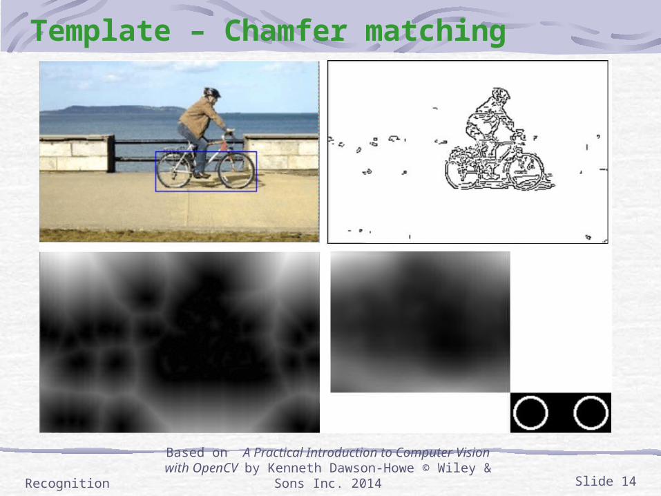
Template – Chamfer matching
RecognitionBased on A Practical Introduction to Computer Vision with
OpenCV by Kenneth Dawson-Howe © Wiley & Sons Inc. 2014 Slide 14
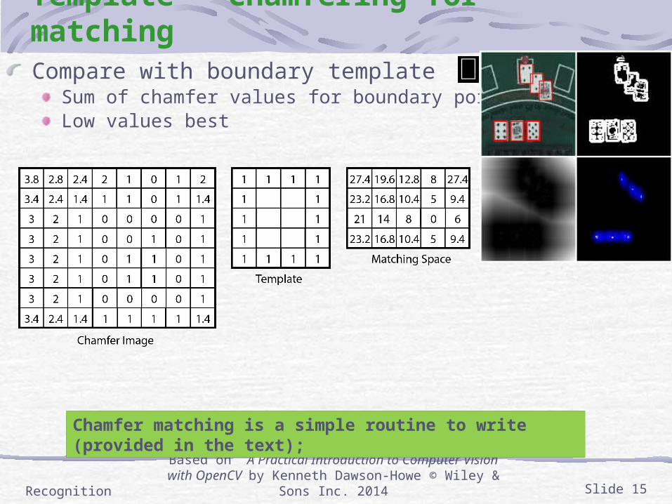
Template – Chamfering for matchingCompare with boundary template
Sum of chamfer values for boundary pointsLow values best
RecognitionBased on A Practical Introduction to Computer Vision with
OpenCV by Kenneth Dawson-Howe © Wiley & Sons Inc. 2014 Slide 15
Chamfer matching is a simple routine to write (provided in the text);
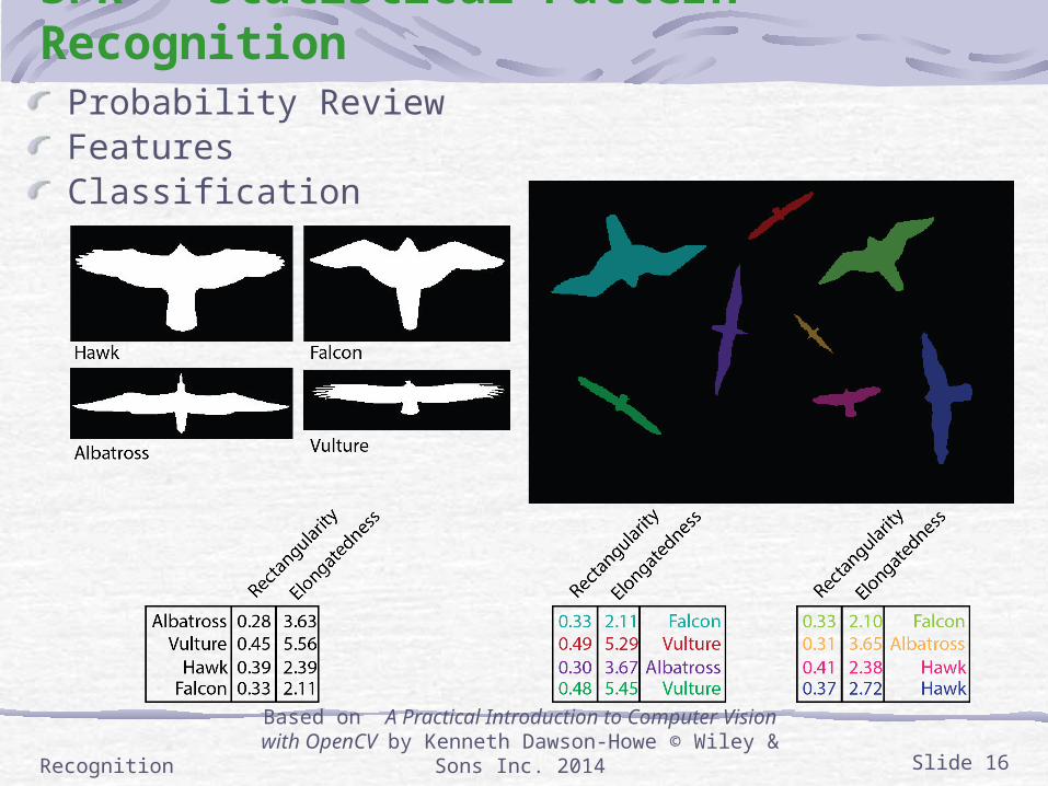
SPR – Statistical Pattern RecognitionProbability ReviewFeaturesClassification
RecognitionBased on A Practical Introduction to Computer Vision with
OpenCV by Kenneth Dawson-Howe © Wiley & Sons Inc. 2014 Slide 16
SPR – Probabitity Review – BasicsP(A) = limn N(A) / nProbability of two events A and B:
Independent: P(AB) = P(A)P(B)
Dependent:P(AB) = P(A|B)P(B)
Conditional Probability P(A|B)
Typical problem:Given some evidence x from an unknown object.What class Wi is the object?Training
A-priori probability – p(x | Wi)Relative probability – p(Wi)
A-posteriori probability – p(Wi | x)
RecognitionBased on A Practical Introduction to Computer Vision with
OpenCV by Kenneth Dawson-Howe © Wiley & Sons Inc. 2014 Slide 17
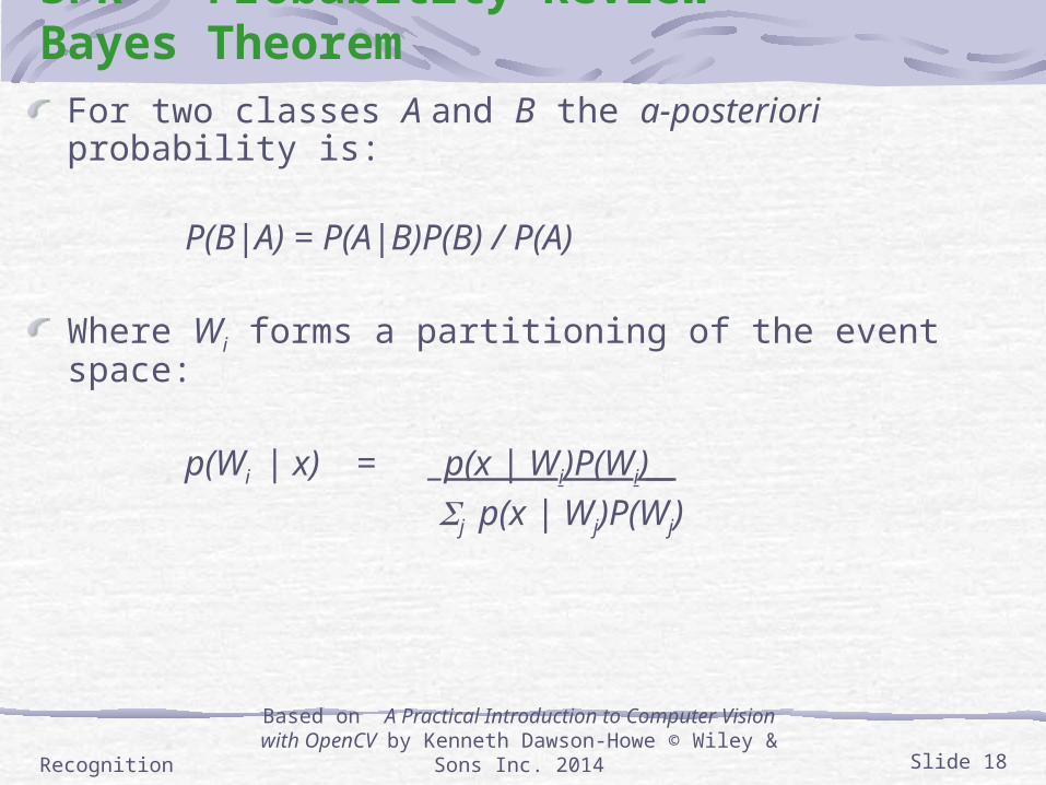
SPR – Probabitity Review – Bayes TheoremFor two classes A and B the a-posteriori probability is:
P(B|A) = P(A|B)P(B) / P(A)
Where Wi forms a partitioning of the event space:
p(Wi | x) = _p(x | Wi)P(Wi)__ j p(x | Wj)P(Wj)
RecognitionBased on A Practical Introduction to Computer Vision with
OpenCV by Kenneth Dawson-Howe © Wiley & Sons Inc. 2014 Slide 18
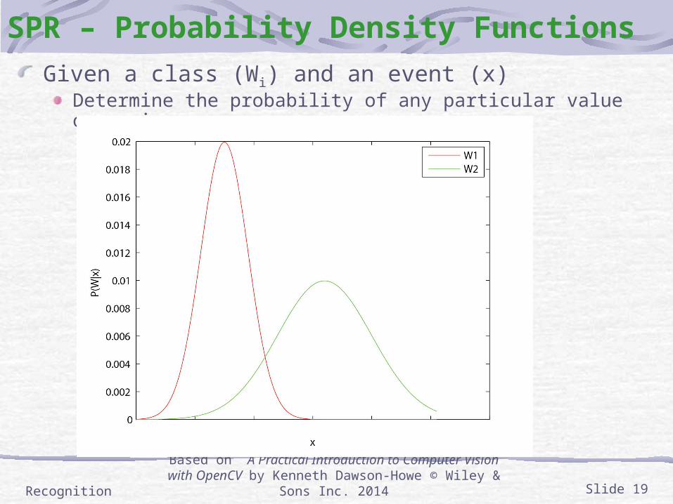
SPR – Probability Density FunctionsGiven a class (Wi) and an event (x)
Determine the probability of any particular value occurring…
RecognitionBased on A Practical Introduction to Computer Vision with
OpenCV by Kenneth Dawson-Howe © Wiley & Sons Inc. 2014 Slide 19
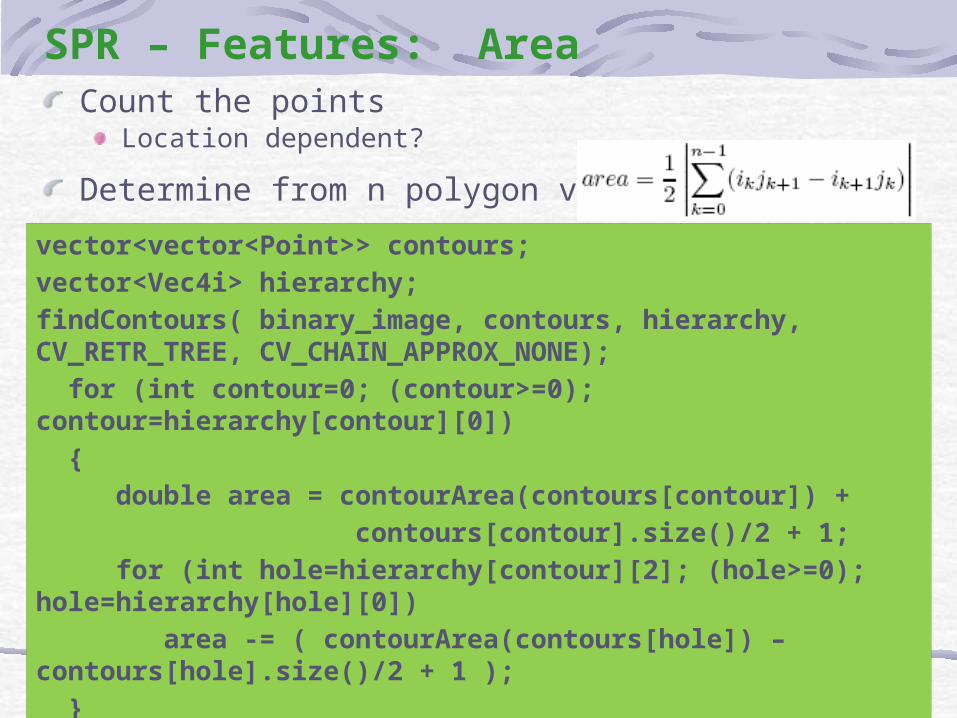
SPR – Features: Area Count the points
Location dependent?
Determine from n polygon vertices
RecognitionBased on A Practical Introduction to Computer Vision with
OpenCV by Kenneth Dawson-Howe © Wiley & Sons Inc. 2014 Slide 20
vector<vector<Point>> contours;
vector<Vec4i> hierarchy;
findContours( binary_image, contours, hierarchy, CV_RETR_TREE, CV_CHAIN_APPROX_NONE);
for (int contour=0; (contour>=0); contour=hierarchy[contour][0])
{
double area = contourArea(contours[contour]) +
contours[contour].size()/2 + 1;
for (int hole=hierarchy[contour][2]; (hole>=0); hole=hierarchy[hole][0])
area -= ( contourArea(contours[hole]) – contours[hole].size()/2 + 1 );
}
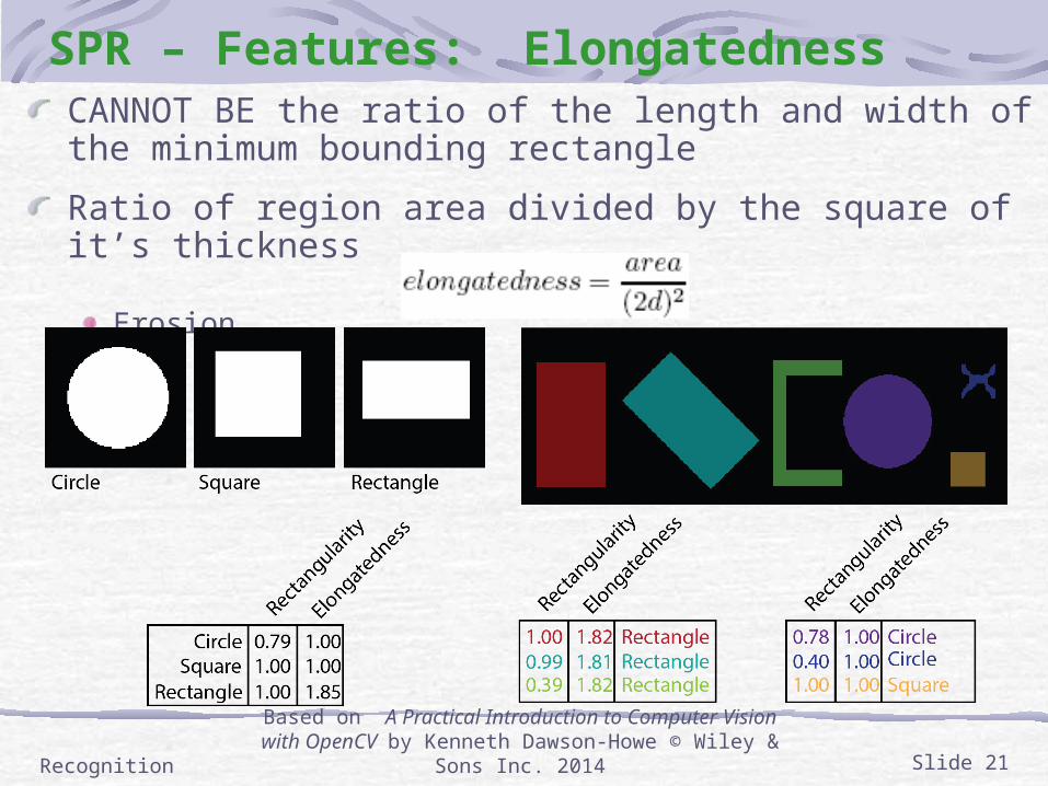
CANNOT BE the ratio of the length and width of the minimum bounding rectangle
Ratio of region area divided by the square of it’s thickness
Erosion
SPR – Features: Elongatedness
RecognitionBased on A Practical Introduction to Computer Vision with
OpenCV by Kenneth Dawson-Howe © Wiley & Sons Inc. 2014 Slide 21
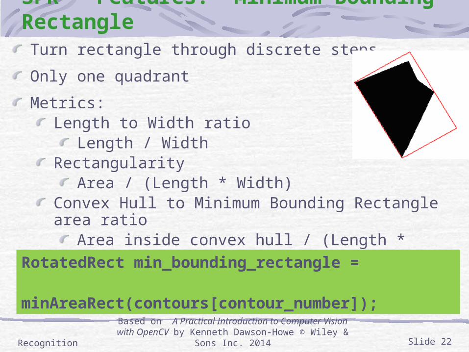
SPR – Features: Minimum Bounding Rectangle Turn rectangle through discrete steps
Only one quadrant
Metrics:Length to Width ratio
Length / WidthRectangularity
Area / (Length * Width)Convex Hull to Minimum Bounding Rectangle area ratio
Area inside convex hull / (Length * Width)
RecognitionBased on A Practical Introduction to Computer Vision with
OpenCV by Kenneth Dawson-Howe © Wiley & Sons Inc. 2014 Slide 22
RotatedRect min_bounding_rectangle =
minAreaRect(contours[contour_number]);
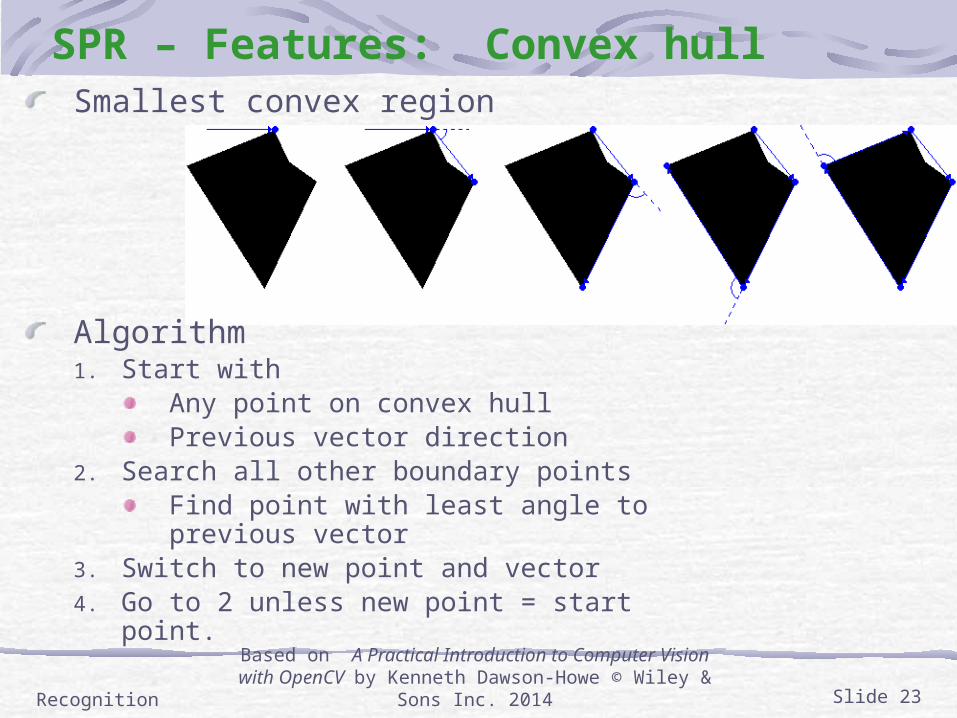
SPR – Features: Convex hull Smallest convex region
Algorithm1. Start with
Any point on convex hullPrevious vector direction
2. Search all other boundary pointsFind point with least angle to previous vector
3. Switch to new point and vector4. Go to 2 unless new point = start point.
RecognitionBased on A Practical Introduction to Computer Vision with
OpenCV by Kenneth Dawson-Howe © Wiley & Sons Inc. 2014 Slide 23

SPR – Features: Convex hull
RecognitionBased on A Practical Introduction to Computer Vision with
OpenCV by Kenneth Dawson-Howe © Wiley & Sons Inc. 2014 Slide 24
vector<vector<Point>> hulls(contours.size());
for (int contour=0; (contour<contours.size()); contour++)
{
convexHull(contours[contour], hulls[contour]);
}
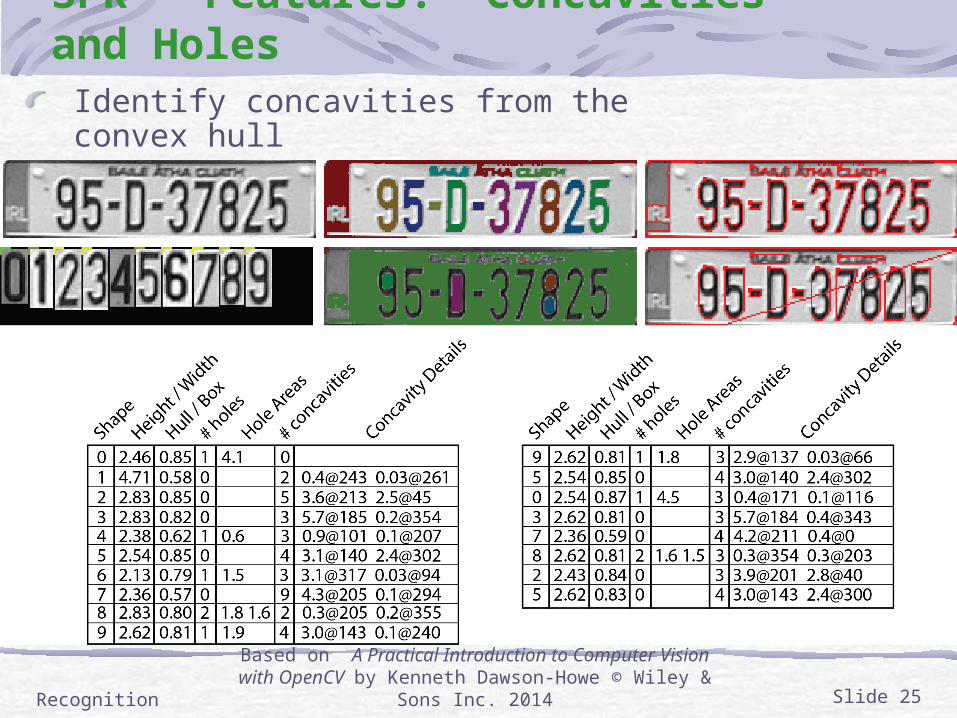
SPR – Features: Concavities and Holes Identify concavities from the convex hullIdentify holes in the binary shape
RecognitionBased on A Practical Introduction to Computer Vision with
OpenCV by Kenneth Dawson-Howe © Wiley & Sons Inc. 2014 Slide 25
SPR – Features: Concavities and Holes
RecognitionBased on A Practical Introduction to Computer Vision with
OpenCV by Kenneth Dawson-Howe © Wiley & Sons Inc. 2014 Slide 26
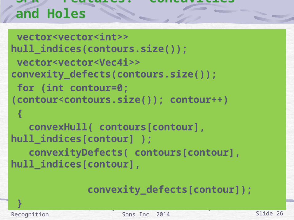
vector<vector<int>> hull_indices(contours.size());
vector<vector<Vec4i>> convexity_defects(contours.size());
for (int contour=0; (contour<contours.size()); contour++)
{
convexHull( contours[contour], hull_indices[contour] );
convexityDefects( contours[contour], hull_indices[contour],
convexity_defects[contour]);
}
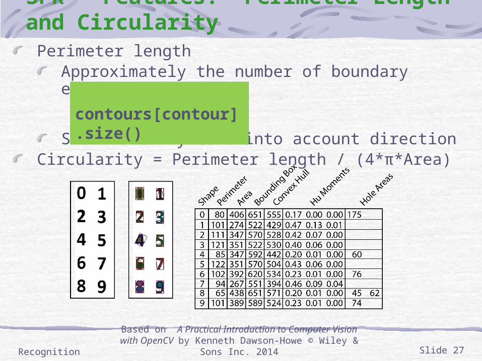
SPR – Features: Perimeter Length and CircularityPerimeter length
Approximately the number of boundary elements
Should really take into account directionCircularity = Perimeter length / (4*π*Area)
RecognitionBased on A Practical Introduction to Computer Vision with
OpenCV by Kenneth Dawson-Howe © Wiley & Sons Inc. 2014 Slide 27
contours[contour].size()
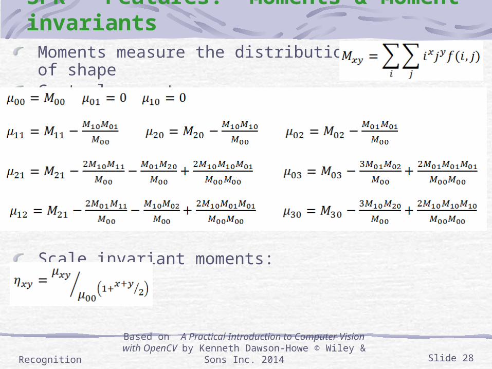
SPR – Features: Moments & Moment invariantsMoments measure the distribution of shapeCentral moments:
Scale invariant moments:
RecognitionBased on A Practical Introduction to Computer Vision with
OpenCV by Kenneth Dawson-Howe © Wiley & Sons Inc. 2014 Slide 28
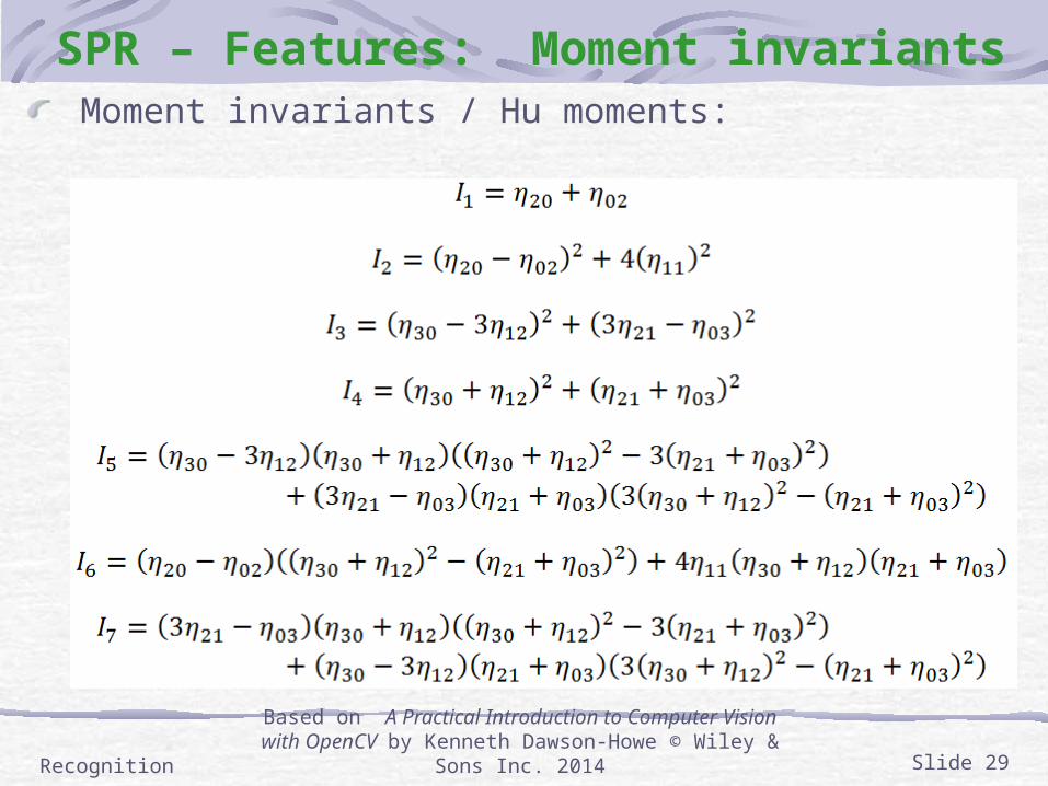
SPR – Features: Moment invariantsMoment invariants / Hu moments:
RecognitionBased on A Practical Introduction to Computer Vision with
OpenCV by Kenneth Dawson-Howe © Wiley & Sons Inc. 2014 Slide 29
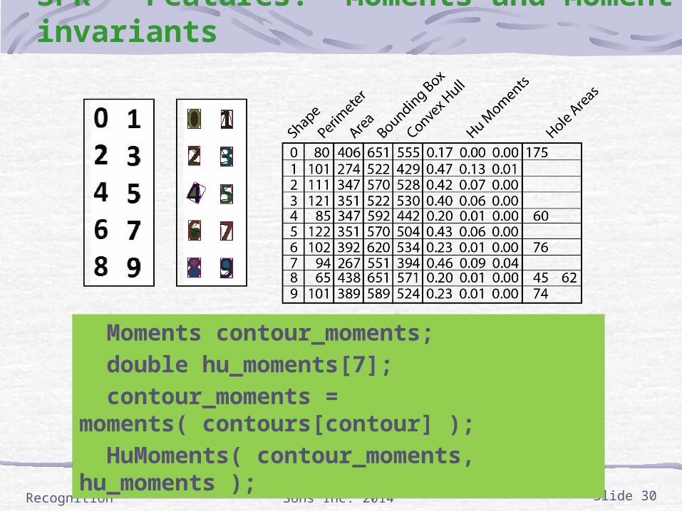
SPR – Features: Moments and Moment invariants
RecognitionBased on A Practical Introduction to Computer Vision with
OpenCV by Kenneth Dawson-Howe © Wiley & Sons Inc. 2014 Slide 30
Moments contour_moments;
double hu_moments[7];
contour_moments = moments( contours[contour] );
HuMoments( contour_moments, hu_moments );
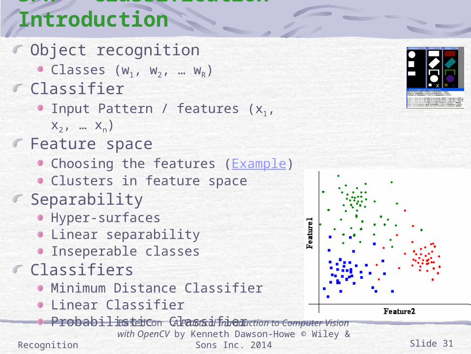
SPR – Classification – Introduction Object recognition
Classes (w1, w2, … wR)Classifier
Input Pattern / features (x1, x2, … xn)Feature space
Choosing the features (Example)Clusters in feature space
SeparabilityHyper-surfacesLinear separabilityInseperable classes
ClassifiersMinimum Distance ClassifierLinear ClassifierProbabilistic Classifier
RecognitionBased on A Practical Introduction to Computer Vision with
OpenCV by Kenneth Dawson-Howe © Wiley & Sons Inc. 2014 Slide 31
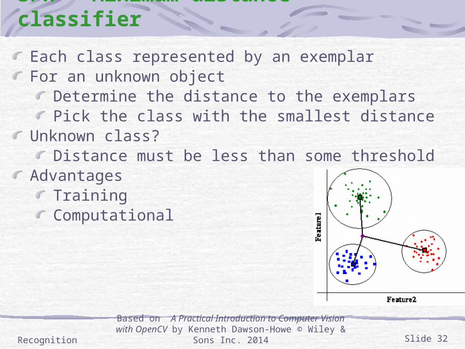
SPR – Minimum distance classifier
Each class represented by an exemplarFor an unknown object
Determine the distance to the exemplarsPick the class with the smallest distance
Unknown class?Distance must be less than some threshold
AdvantagesTrainingComputational
RecognitionBased on A Practical Introduction to Computer Vision with
OpenCV by Kenneth Dawson-Howe © Wiley & Sons Inc. 2014 Slide 32
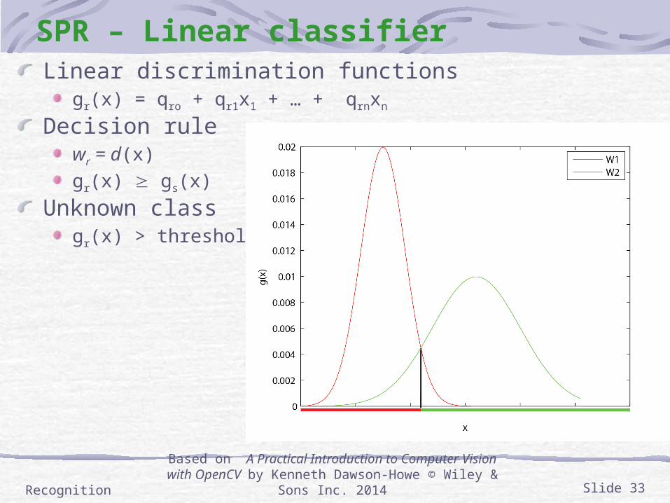
SPR – Linear classifierLinear discrimination functions
gr(x) = qro + qr1x1 + … + qrnxn
Decision rulewr = d(x)gr(x) gs(x)
Unknown classgr(x) > threshold
RecognitionBased on A Practical Introduction to Computer Vision with
OpenCV by Kenneth Dawson-Howe © Wiley & Sons Inc. 2014 Slide 33
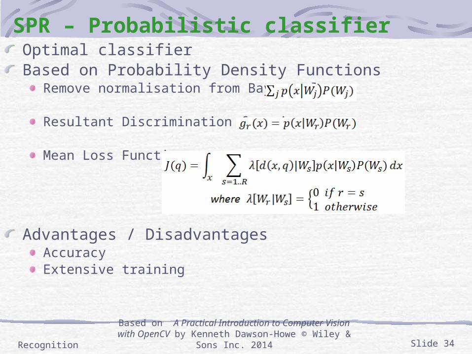
SPR – Probabilistic classifierOptimal classifierBased on Probability Density Functions
Remove normalisation from Bayes rule…
Resultant Discrimination function:
Mean Loss Function:
Advantages / DisadvantagesAccuracyExtensive training
RecognitionBased on A Practical Introduction to Computer Vision with
OpenCV by Kenneth Dawson-Howe © Wiley & Sons Inc. 2014 Slide 34
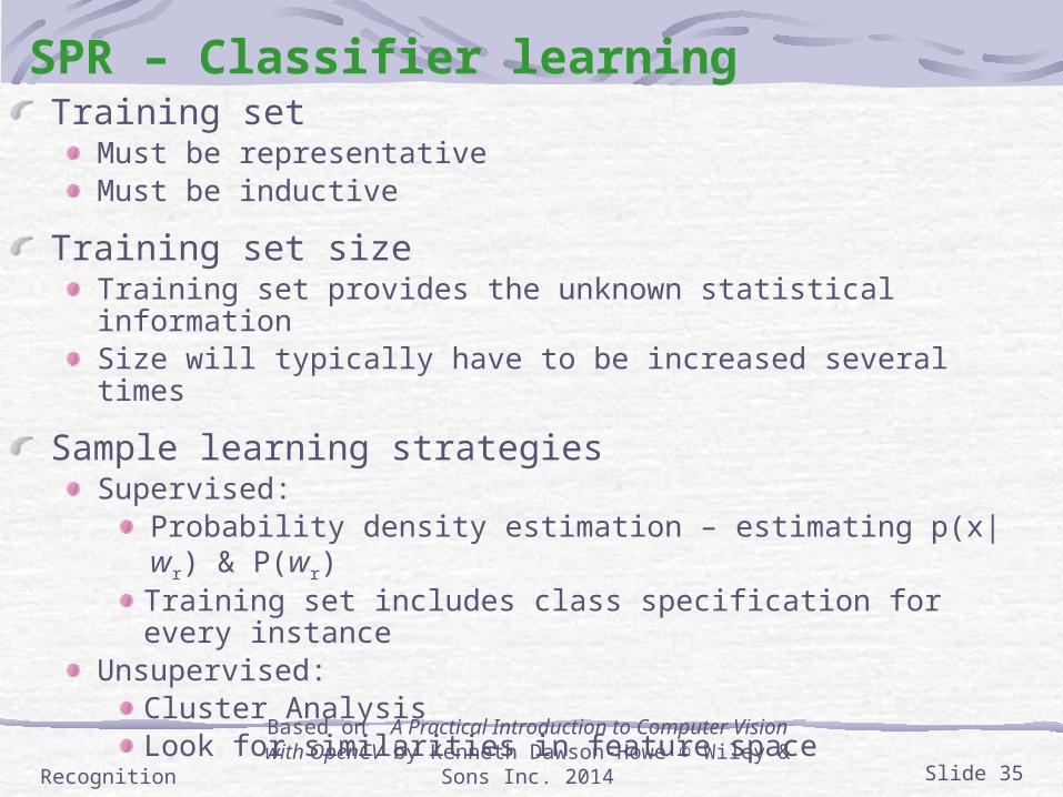
SPR – Classifier learningTraining set
Must be representativeMust be inductive
Training set sizeTraining set provides the unknown statistical information Size will typically have to be increased several times
Sample learning strategiesSupervised:
Probability density estimation – estimating p(x|wr) & P(wr) Training set includes class specification for every instance
Unsupervised:Cluster AnalysisLook for similarities in feature space
RecognitionBased on A Practical Introduction to Computer Vision with
OpenCV by Kenneth Dawson-Howe © Wiley & Sons Inc. 2014 Slide 35
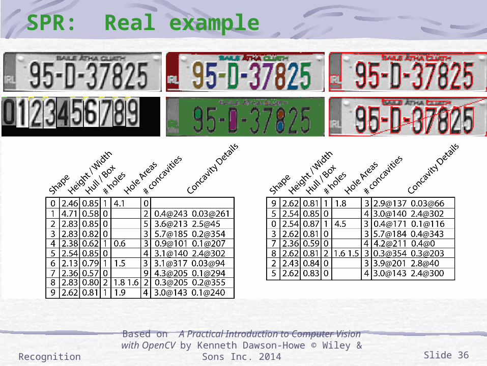
SPR: Real example
RecognitionBased on A Practical Introduction to Computer Vision with
OpenCV by Kenneth Dawson-Howe © Wiley & Sons Inc. 2014 Slide 36
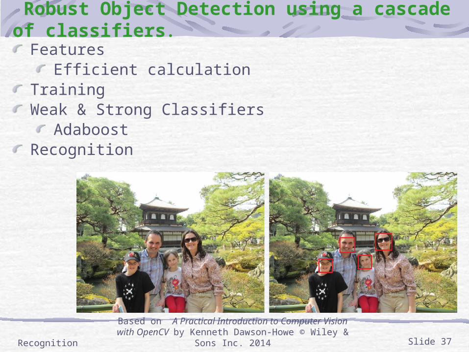
Haar – Robust Object Detection using a cascade of classifiers.
FeaturesEfficient calculation
TrainingWeak & Strong Classifiers
AdaboostRecognition
RecognitionBased on A Practical Introduction to Computer Vision with
OpenCV by Kenneth Dawson-Howe © Wiley & Sons Inc. 2014 Slide 37
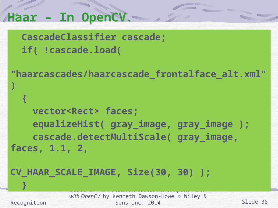
Haar – In OpenCV.
RecognitionBased on A Practical Introduction to Computer Vision with
OpenCV by Kenneth Dawson-Howe © Wiley & Sons Inc. 2014 Slide 38
CascadeClassifier cascade;
if( !cascade.load(
"haarcascades/haarcascade_frontalface_alt.xml" )
{
vector<Rect> faces;
equalizeHist( gray_image, gray_image );
cascade.detectMultiScale( gray_image, faces, 1.1, 2,
CV_HAAR_SCALE_IMAGE, Size(30, 30) );
}
Haar – OverviewTraining using a number of positive and negative samples
Uses simple (Haar like) featuresEfficient calculation…
Selects a large number of these features during training to create strong classifiers
Links a number of strong classifiers into a cascade for recognitionEfficiency…
Can work at different scales
RecognitionBased on A Practical Introduction to Computer Vision with
OpenCV by Kenneth Dawson-Howe © Wiley & Sons Inc. 2014 Slide 39

Haar – FeaturesFeatures determined as the difference of the sums of a number of rectangular regions
Place the mask in a specific locationand at a specific scaleThen subtract the sum of the ‘white pixels’from the sum of the ‘black pixels’
Why does this work?
RecognitionBased on A Practical Introduction to Computer Vision with
OpenCV by Kenneth Dawson-Howe © Wiley & Sons Inc. 2014 Slide 40
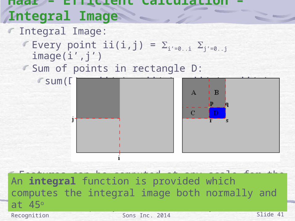
Haar – Efficient Calculation – Integral ImageIntegral Image:
Every point ii(i,j) = i’=0..i j’=0..j image(i’,j’)Sum of points in rectangle D:
sum(D) = ii(p) + ii(s) – ii(q) – ii(r)
Features can be computed at any scale for the same cost
RecognitionBased on A Practical Introduction to Computer Vision with
OpenCV by Kenneth Dawson-Howe © Wiley & Sons Inc. 2014 Slide 41
An integral function is provided which computes the integral image both normally and at 45o
Haar – TrainingNumber of possible features.
the variety of feature typesallowed variations in size and position
Training mustIdentify the best features to use at each stageTo do this positive and negative samples are needed…
RecognitionBased on A Practical Introduction to Computer Vision with
OpenCV by Kenneth Dawson-Howe © Wiley & Sons Inc. 2014 Slide 42
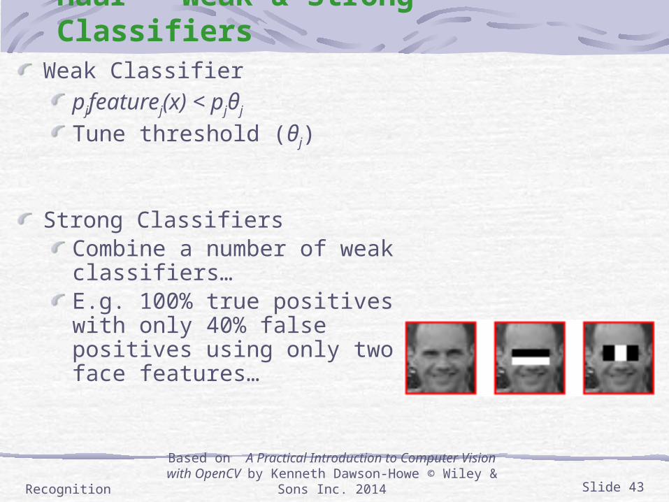
Haar – Weak & Strong ClassifiersWeak Classifier
pjfeaturej(x) < pjθj Tune threshold (θj)
Strong ClassifiersCombine a number of weak classifiers…E.g. 100% true positives with only 40% false positives using only two face features…
RecognitionBased on A Practical Introduction to Computer Vision with
OpenCV by Kenneth Dawson-Howe © Wiley & Sons Inc. 2014 Slide 43
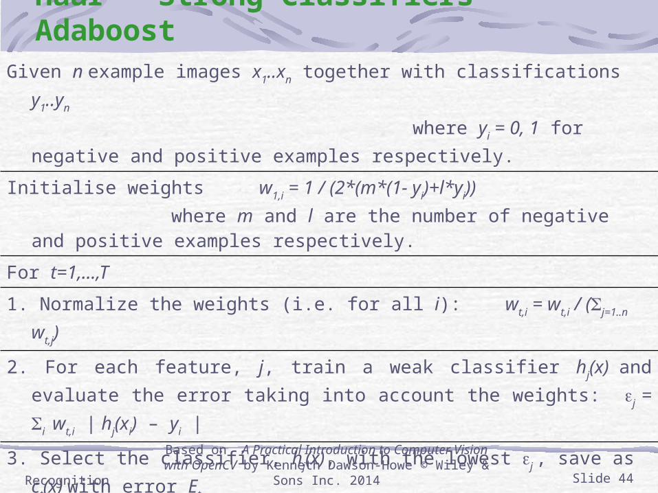
Haar – Strong Classifiers – AdaboostGiven n example images x1..xn together with classifications y1..yn
where yi = 0, 1 for negative and positive examples respectively.
Initialise weights w1,i = 1 / (2*(m*(1- yi)+l*yi)) where m and l are the number of negative and positive examples respectively.
For t=1,…,T
1. Normalize the weights (i.e. for all i): wt,i = wt,i / (j=1..n wt,j)
2. For each feature, j, train a weak classifier hj(x) and evaluate the error taking into account the weights: j = i wt,i | hj(xi) – yi |
3. Select the classifier, hj(x), with the lowest j , save as ct(x) with error Et
4. Update the weights (i.e. for all i): wt+1,i = wt,i t(1- ei )
where ei = | ct(xi) – yi | and t = Et / (1–Et)
The final strong classifier is: h(x)= 1 if t=1..T αtct(x) ½ t=1..T αt ,
0 otherwise where αt = log 1/t
RecognitionBased on A Practical Introduction to Computer Vision with
OpenCV by Kenneth Dawson-Howe © Wiley & Sons Inc. 2014 Slide 44
Haar – Classifier cascadeObject recognition is possible with a single strong classifier
To improve detection rates AND to reduce computation time:A cascade of strong classifiers can be usedEach stage either accepts or rejectsOnly those accepted pass to the next stage
Efficient computation…
Strong classifiers trained using AdaBoostOn the remaining set of data
RecognitionBased on A Practical Introduction to Computer Vision with
OpenCV by Kenneth Dawson-Howe © Wiley & Sons Inc. 2014 Slide 45
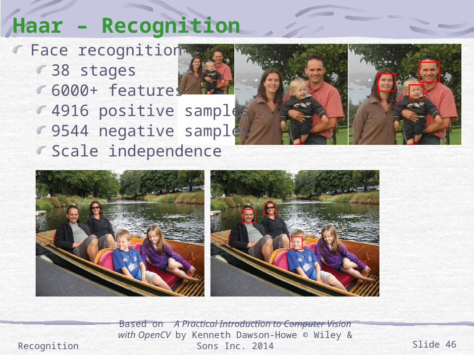
Haar – RecognitionFace recognition
38 stages6000+ features4916 positive samples9544 negative samplesScale independence
RecognitionBased on A Practical Introduction to Computer Vision with
OpenCV by Kenneth Dawson-Howe © Wiley & Sons Inc. 2014 Slide 46
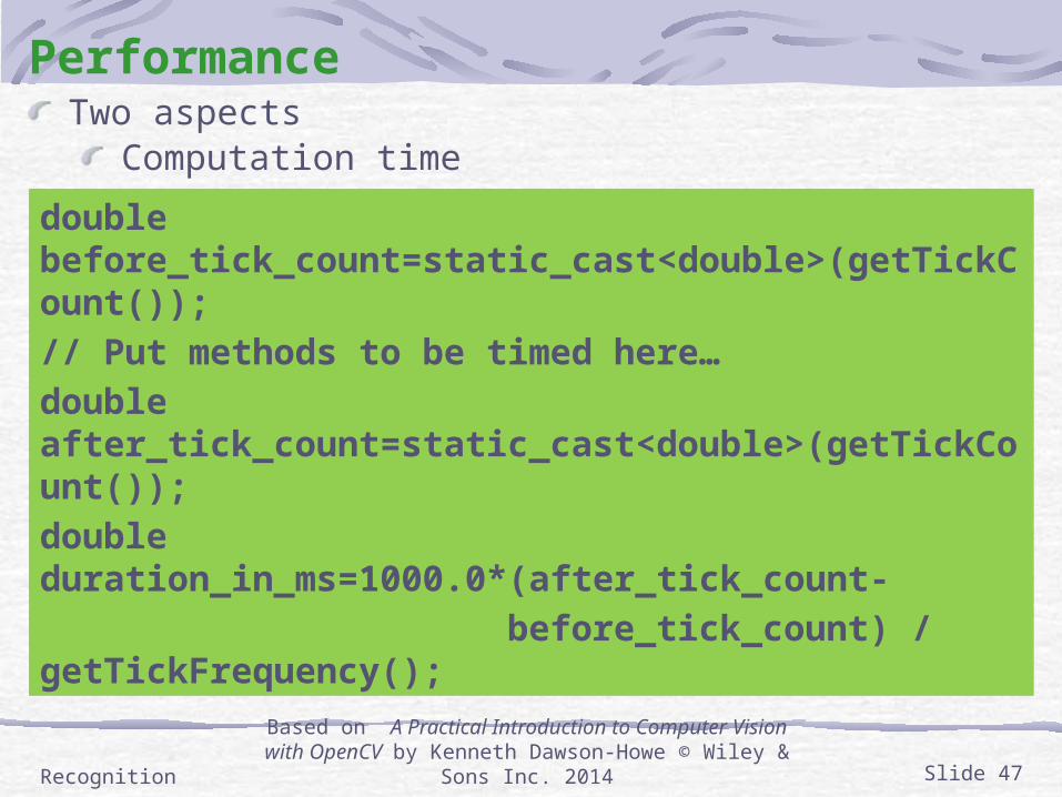
PerformanceTwo aspects
Computation time
Success and failure ratesWhat is the correct answer?
We need ground truthHow do we assess success?
We need metrics.
RecognitionBased on A Practical Introduction to Computer Vision with
OpenCV by Kenneth Dawson-Howe © Wiley & Sons Inc. 2014 Slide 47
double before_tick_count=static_cast<double>(getTickCount());
// Put methods to be timed here…
double after_tick_count=static_cast<double>(getTickCount());
double duration_in_ms=1000.0*(after_tick_count-
before_tick_count) / getTickFrequency();
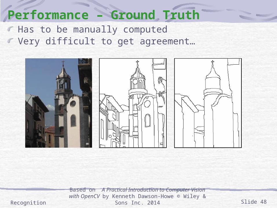
Performance – Ground TruthHas to be manually computedVery difficult to get agreement…
RecognitionBased on A Practical Introduction to Computer Vision with
OpenCV by Kenneth Dawson-Howe © Wiley & Sons Inc. 2014 Slide 48
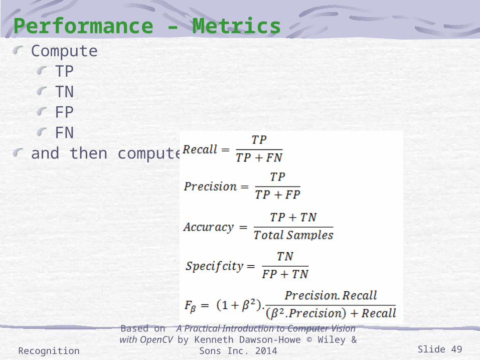
Performance – MetricsCompute
TPTNFPFN
and then compute…
RecognitionBased on A Practical Introduction to Computer Vision with
OpenCV by Kenneth Dawson-Howe © Wiley & Sons Inc. 2014 Slide 49
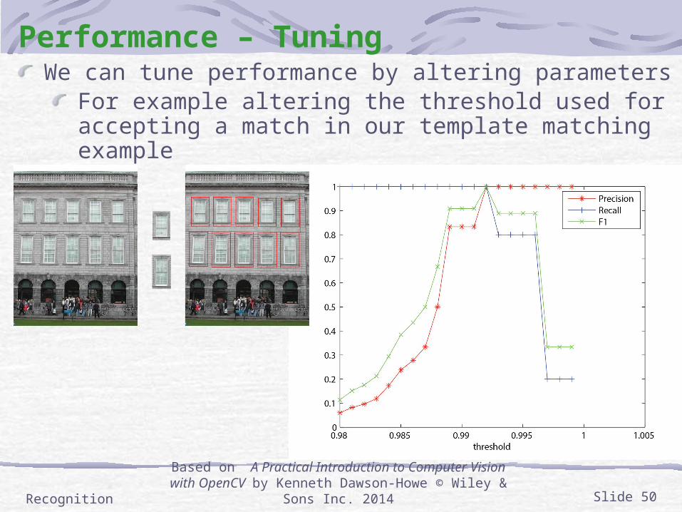
Performance – TuningWe can tune performance by altering parameters
For example altering the threshold used for accepting a match in our template matching example
RecognitionBased on A Practical Introduction to Computer Vision with
OpenCV by Kenneth Dawson-Howe © Wiley & Sons Inc. 2014 Slide 50
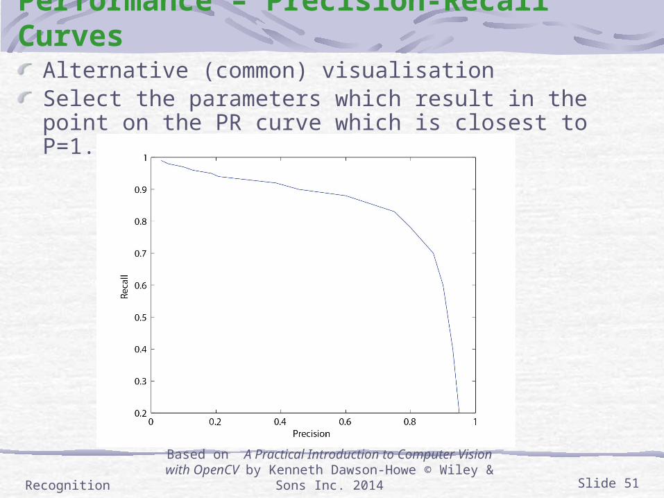
Performance – Precision-Recall CurvesAlternative (common) visualisationSelect the parameters which result in the point on the PR curve which is closest to P=1.0, R=1.0
RecognitionBased on A Practical Introduction to Computer Vision with
OpenCV by Kenneth Dawson-Howe © Wiley & Sons Inc. 2014 Slide 51