social proximity and bureaucrat performance:...

Social Proximity and Bureaucrat Performance:Evidence from India∗

Guo Xu, Marianne Bertrand and Robin Burgess†

February 18, 2018Preliminary draft

Abstract

How does social proximity affect bureaucrat performance? Using exogenous vari-ation in social proximity generated by an allocation rule, we find that bureaucratsassigned to their home states are perceived to be more corrupt and less able to with-stand illegitimate political pressure. These effects are driven by the more corrupt statesand concentrated among officers with higher social proximity within their state. Homestate officers are also more likely to remain in their state, are reshuffled more frequentlyand more likely to serve on the boards of private companies while holding public of-fice. These patterns are consistent with social proximity adversely impacting bureaucratperformance through local capture.

JEL classification: D73, H11, O10

∗Contact details: [email protected] (corresponding author), [email protected],[email protected]. First draft: December 2017.†Marianne Bertrand [University of Chicago Booth School of Business: Mari-

[email protected]]; Robin Burgess [London School of Economics (LSE): [email protected]];Guo Xu [University of Berkeley, Haas School of Business: [email protected]]

1

1 Introduction

Bureaucrats are a key determinant of state capacity (Besley and Persson 2009, Finan et al.2015): they are responsible for raising revenue, providing public services and implementingreforms. Understanding how to improve the allocation of talent within the public sectorcan have potentially large impacts on development and growth.

This paper studies the allocation of talent in organizations by asking how social prox-imity between bureaucrats and their assigned workplace affects performance. In studyingthe role of social proximity in the allocation of talent, we provide empirical evidence on thecentral tension between delegation and control. On the one hand, the principal can assignbureaucrats to socially proximate environments to leverage private information. On theother hand, the principal must retain control so bureaucrats do not abuse their informa-tional advantage for private gain (Aghion and Tirole 1997). This trade-off is particularlyimportant in public organizations, as a defining feature of bureaucrats is their expertise(Niskanen 1971, Banks and Weingast 1992, Alesina and Tabellini 2007).

We study one of the most important bureaucracies: the Indian Administrative Service(IAS). This is the elite civil service of India, comprised of around 3,000 centrally recruitedsenior civil servants who head up the upper echelons of the bureaucracy. These bureau-crats head up all government departments at the state level in India. These officers aretherefore important for the implementation of state-level policies and for providing a reg-ulatory environment conducive to economic growth (Asher and Novosad 2015, Bertrand etal. 2017).

Empirically, we exploit variation in social proximity using plausibly exogenous variationin the assignment of officers to their home state. Social proximity, as captured by geograph-ical distance and shared language, captures key aspects of local information (Fisman et al.2017, Huang et al. 2017). Assigning workers to an area with shared language, culture orvalues may increase performance by allowing workers to harness private information andsocial incentives. Social proximity however may also decrease performance as workers abuselocal networks to engage in corrupt behavior (Ashraf and Bandiera 2017).

Our empirical strategy leverages knowledge of the home state assignment rule to isolatea source of variation that (i) predicts the allocation to home state and (ii) is uncorrelatedwith observable individual background characteristics of the officers. In balancing the aimto equalize the quality of administrators across the states of India and to allow officers toserve in their home state at the same time, the IAS uses a rule-based mechanism to deploynewly recruited officers to states. While higher ranked officers are more likely to be assignedto their home state, we exploit the fact that officers are grouped according to their caste× home state bracket when ranked in the allocation process. This implies that officerswho are the only candidate in their bracket in a given year of intake are allocated to theirhome state with near certainty. Variation in the bracket size, however, depends on whetherofficers from the same caste and state passed the competitive entry exam in the same year.We argue and provide evidence that officers are, conditional on the selection bracket, asgood as randomly assigned to their home state.

2

The main finding is that home state allocated officers perform worse than comparableofficers who are allocated to non-home states. Instrumental variable estimates suggestthat officers allocated to their home state are deemed to be more corrupt and less ableto withstand illegitimate political pressure. This effect is primarily driven by the morecorrupt and less developed home states. The negative home state effect is weaker for higherability officers, as measured using the entry exam scores. Consistent with the evidencefrom subjective ratings, we find that home state officers are less likely to work outside theirstate and subject to more political interference, as measured by shorter job postings andgreater transfers. Finally, by matching IAS officers to company registries, we find that homestate officers are more likely to serve in both public and private boards. These firms arealso more likely to be based in the same state, thus reflecting the officer’s greater accessto local networks. Taken together, the results suggest that social proximity may decreaseperformance by increasing the likelihood of local capture.

These findings are important as the question of how to allocate talent is central inorganizations. Focusing on the one-off and life-long deployment of officers to states allowsus to isolate bureaucrat-workplace match effects, thus providing novel evidence in a settingthat hitherto primarily focused on the incentivizing role of frequent transfers (Iyer and Mani2012, Jia 2015, Xu 2017). Our findings resonate well with the historical literature whichhighlights the tension between the need for local knowledge and the challenge of captureand clientelism in settings ranging from the administration of Empire to the allocation ofmodern day civil servants and ambassadors (Kirk-Greene 2000, Newbury 2003, Greif 2007).1

2 Background and Data

The Indian Administrative Service (IAS), the successor of the Indian Civil Service (ICS), isthe elite administrative civil service of the Government of India.2 In 2014 the IAS had anoverall strength of around 3,600 centrally recruited officers. These officers are civil serviceleaders, occupying key positions critical for policy implementation. The most senior civilservice positions - the Cabinet Secretary of India, the Chief Secretary of States, heads ofall state and federal government departments - are occupied by IAS officers.

The recruitment of officers is based on the performance in the Civil Service Exam, whichis annually organized by the Union Public Service Commission (UPSC). Entry into the IASis extremely competitive, with several hundred thousand applicants competing for a smallnumber of spots. In 2015, for example, 465,882 UPSC exam takers faced only 120 IAS slots.Those who do not qualify for the IAS may obtain positions in less competitive civil servicestreams such as the Indian Police Service (IPS), the Indian Forest Service (IFS), the IndianRevenue Service (IRS) or the state civil services. The highest performing exam takers are

1In Imperial China, for example, the “rule of avoidance” prevented district magistrates to serve in theirhome districts during the Sui Dynasty. The issue of local capture in the US Foreign Service, for example, isreferred to as ”localitis” and frequent rotation has been mentioned as a means to prevent local entrenchment(Jonsson and Hall 2005). Steiner (2015) describes the historical challenge to ”balance the need for linguisticsand regional expertise against the dangers of ’localitis’ and excessive isolation.”

2The description of the study setting and context borrows heavily from Bertrand et al. 2017.

3

typically offered slots in the IAS. There are quotas for the reserved castes, namely the OtherBackward Castes (OBC), Scheduled Castes (SC) and Scheduled Tribes (ST). Once selected,IAS officers are allocated to a state cadre. The assignment to a state is typically fixed forlife,3and officers are attached to their state cadre even when serving in Delhi or abroad. Afterselection and allocation to a state cadre, IAS officers undergo training at the Lal BahadurShastri National Academy of Administration (LBSNAA) and in the states. The two-yeartraining consists of one year academic training at the LBSNAA (“course work”) and oneyear practical training (“district training”). After training, recruits are initially placed inthe district administration (e.g. as district collectors), and are subsequently promoted tohigher level positions. Finally, retirement occurs at 60 years of age for both male and femaleofficers (58 years before 1998).

2.1 Data and empirical setting

We leverage several datasets for our study. The main dataset on performance indicatorsand background characteristics comes from Bertrand et al. (2017).

Subjective performance ratings. Bertrand et al. (2017) introduce a new frameworkto measure the performance of civil servants based on subjective performance ratings. Per-formance scores were collected for a cross-section of centrally recruited IAS officers workingin the 14 major states of India4 with at least 8 years of tenure. These scores were providedby a wide range of stakeholders in each state, ranging from IAS officers, state civil servants,politicians (MLA) to representatives of media, business and NGOs. Each officer was scoredon a scale of 1 (low) to 5 (high), covering five dimensions of performance: effectiveness,probity, the ability to withstand illegitimate political pressure, pro-poor orientedness andoverall performance. Overall, the survey covered 1,450 bureaucrats who were serving in2012-13 and with at least 8 years of tenure. This corresponds to a coverage rate of 71%.

Administrative data. We link the survey data on performance with administrativedata from the descriptive rolls, the inter-se-seniority lists and the executive sheets. Thedescriptive rolls contain a rich set of individual background characteristics for 5,635 officerswho entered between 1975-2005. Characteristics range from year of birth, their home state,caste, family background, educational degrees and work experience. The inter-se-senioritylists cover 4,107 officers from 1972-2009. This dataset provides information about theallocation of officers to states as well as their scores on the entry exam, training course andoverall rank. Finally, the executive record sheets cover the postings of 10,817 IAS officerswho entered between 1949-2014. These records contain detailed information about postingsand payscales, allowing us to track the progression of IAS officers over time. After linkingall sources, the final dataset covers up to 1,888 IAS officers who entered between 1976-2005.

Table 1 reports the mean and standard deviation of the performance scores. The samplesizes range from N = 15, 153 for the probity measure to N = 17, 753 for the effectiveness

3The only exception for transfers across states in in the case of marriage to another IAS officer. Thesecases, however, have to be approved on case-by-case basis and are rare.

4These are: Andhra Pradesh, Bihar, Gujarat, Haryana, Karnataka, Kerala, Madhya Pradesh, Maharash-tra, Orissa, Punjab, Rajasthan, Tamil Nadu, Uttar Pradesh and West Bengal.

4

measure. The number of complete assessments across all dimensions is N = 14, 037. Wewere able to elicit scores for about 70% of all IAS officers in our sample. All dimensions arecorrelated, with the highest correlation being between pro-poor orientation and the abilityto withstand illegitimate political pressure.

Table 2 compares the average individual characteristics of officers who are allocated totheir home state vs. those who are not. The sample comprises all IAS officers who enteredbetween 1975-2005. The table compares both the raw average (Column 3) and the averagedifference within each year of intake (Column 4). In accordance with the merit-based homestate allocation, home state allocated officers tend to rank, on average, higher. Within agiven intake, officers who receive their home state rank on average 17 positions higher thanthose who do not. The non-random allocation for home state officers also translates intosignificant differences on other margins: home state allocated officers are, on average, lesslikely to be from the Other Backward Castes and more likely from Scheduled Castes. Moregenerally, a joint hypothesis test rejects the null that home state allocated officers are, onaverage, comparable to non-home state officers.

2.2 Allocation Rule

We describe the rule governing the allocation of IAS officers to state cadres in detail asthis will generate the critical source of variation.5 We focus on the allocation rule that hasbeen in place between throughout most of the cohorts 1984-2005. The allocation follows astrict rule-based procedure. After entering the IAS following the UPSC exams, centrallyrecruited IAS officers are allocated to 24 cadres. These cadres typically map directly intothe Indian states.6 The allocation process can be broadly divided into three steps: In thefirst step, IAS applicants are asked to declare their preference to remain in their home state(referred to as insider preference). In the second step, the overall number of vacancies andthe corresponding quotas for castes and insiders are determined. In the final step, vacanciesand officers are matched in the actual allocation process.

Step 1. IAS officers declare their cadre preferences by first stating their preference toremain in their state of residence. For the year where we observe the home state declaration(2006), nearly all IAS officers exercise this option. The declared preferences however do notguarantee the actual allocation as the assignment depends on the availability of vacancies.

Step 2. The total number of vacancies is determined by the state government withthe Department of Personnel and Training. Typically, the overall number of vacancies ina given year depend on the shortfall from the total number of IAS officers designated to astate (the cadre strength). This cadre strength is defined by the ”cadre strength fixationrules”, whereby larger states are assigned more IAS officers. These rules are seldom revised

5The exact documentation can be found in the IAS guidelines. Refer to the original official notifications:13013/2/2010-AIS-I, 29062/1/2011-AIS-I and 13011/22/2005-AIS-I published in the Department of Person-nel and Training, Ministry of Personnel, Public Grievances and Pensions, Government of India. Note thatwe describe the dominant allocation rule in our study period 1976-2005. The rule was reformed in 2008.

6Smaller states, however, are grouped into three joint cadres, which are Assam-Meghalaya, Manipur-Tripura and AGMUT (Arunachal Pradesh, Goa, Mizoram and Union Territories (Delhi)). We did notsurvey states with pooled cadres due to logistical constraints.

5

so the designated state cadre strength is fixed over longer periods. The vacancies arethen broken down by quotas on two dimensions: caste and home preference. There arethree categories for castes: General (unreserved) caste, Scheduled Caste/Tribes (SC/ST)and Other Backward Castes (OBC). The designation of vacancies to these caste categoriesare made based on predefined national quotas. The actual assignment of each vacancyto a caste is randomized using a rotating roster. In terms of preferences, vacancies arebroken down into ”insider” and ”outsider” vacancies. Insider vacancies are to be filledby IAS officers from the same state who declared their home state preference at timeof application. The ratio of insider to outsider vacancies is 1:2, with the assignment ofvacancies to ”insider” or ”outsider” category following the repeating sequence O-I-O. Thedetermination of vacancies is illustrated in Appendix Figure A1. The result of this procedureis a list denoting the number of vacancies for each state and the corresponding quotas bycaste status (SC/ST/OBC) and home state (insider/outsider) as shown in Appendix FigureA2.

Step 3. The final allocation process is based on merit as determined by the ranking inthe UPSC entry exam, the vacancies available and the preference stated. Before the officersare allocated, the candidates are ranked and assigned a serial number in the order of merit,as determined by the UPSC exam. Appendix Figure A3 shows this ranking along withthe officers’ caste and home preference. The highest scoring candidate for the 2006 intake,for example, was Mutyalaraju Revu who belongs to the OBC category and indicated hispreference to be assigned to his home state Andhra Pradesh.

Home state assignment. The insider vacancies are allocated as far as exact matchesalong caste and home state preference (the allocation ”bracket”) permit. If the number ofmatches exceed the vacancies, the higher ranking IAS officer is given preference. Given theexact match along caste and home state required for slotting, however, many insider va-cancies typically remain unfilled. In this case, the caste requirement is successively relaxed,eventually opening to outsiders.7

Non-home state assignment. The allocation of the ”outsiders” and those who failedto be allocated to their preferred home state (and are consequently converted to outsiders)is done according to a rotating roster system. In a nutshell, the rotating roster is designedto ensure that each state receives, on average, candidates of similar quality across years.8

The critical feature for our empirical strategy is that home state officers are grouped andranked within caste × home state brackets in each year of intake. The size of the bracketwill vary across years depending on how many candidates from the same home state andcaste pass the entry exam. This is the identifying source of variation we exploit. Whilethe allocation rule for outsiders saw minor adjustments over time, this feature of the homestate allocation has remained constant throughout the cohorts we study.9

7The exact details are not directly relevant for our identification strategy and are therefore omitted forbrevity. For completeness, refer to Appendix C.1.

8Again, the exact details are not directly relevant for our identification strategy and we therefore referto Appendix C.2.

9Between 1978-1984, officers were allowed to also declare preferred “zones” (i.e. groups of states) forthe outsider allocation (the “Limited Zonal Preference System”). After 2008 (and thus beyond our study

6

3 Determinants of home state allocation

3.1 Empirical strategy

The key empirical challenge to estimating the causal effect of home state allocations isthat the assignment of IAS candidates to home cadres is, unlike the overall assignmentrule, non-random. Indeed, under the allocation rule outlined above, higher ranked IASofficers are given priority in their declared preference to be allocated to their home state.As higher ranked officers are prioritized for their home state allocation (Bhavnani and Lee2017), a simple comparison between home state vs. non home state officers is likely to yieldupwardly biased estimates of the effect of home allocation on bureaucratic performance. Wetherefore require an instrument that predicts the likelihood of an officer receiving a homestate allocation, but that is otherwise not correlated with the outcomes of interest.

Our empirical strategy exploits knowledge of the rule-based home state allocation: weargue that home state allocation is, conditional on the allocation rule, as good as randomlyassigned. Specifically, we predict home state allocation using the fact that the ranking ofIAS officers for home state allocation occurs within pre-defined brackets. Instead of givingofficers priority in their home state preference in descending order of their overall rank,officers are ranked within ”brackets” based on their year of intake, home state and caste(e.g. 2015-Gujarat-OBC). Depending on corresponding vacancies, officers are then slottedwithin descending order of rank within their bracket.

One important implication of this rule is that there will be variation in the numberof officers who are competing for home state allocations in the same bracket over time.To illustrate this, Figure 1 plots the share of home state allocations and the number ofcandidates for the Uttar Pradesh-Scheduled Caste bracket for different years of intake.As the figure shows, of course, home state allocations never occur in years when there isno scheduled caste candidate from Uttar Pradesh. More importantly, it is apparent fromthe figure that whether or not an IAS officer gets assigned to his or her home state is(mechanically) negatively correlated to the total number of officers in the same bracket.10

More generally, Figure 2 plots the probability of a home state allocation for a givenofficer as a function of the number of candidates in the same bracket relative to being asingle candidate. Compared to a single candidate, having another candidate in the samebracket decreases the probability of a home state allocation by 15% points. The probabilityis 54% points lower when facing more than 8 other candidates. Most of the variation inthe number of candidates, however, occurs between a single and two candidates. 42% ofthe allocation brackets comprise only a single candidate, and 21% contain two candidates.Only 9.6% of the brackets contain more than 8 candidates.11

In light of this, we propose to predict home state allocation using a dummy that equals 1if the officer is the only candidate in his or her year of intake-home state and caste bracket,

period), officers were allowed to declare their preferences beyond a home state allocation by ranking thestates in their preferred order (the “Merit-cum-preference system”).

10Appendix Figures A5 to A8 summarize the variation across time for all states and caste bins.11These brackets are located in large states such as Uttar Pradesh. See Appendix Table B1 for a summary

of the bracket sizes by states.

7

0 otherwise. This captures not only the most relevant margin of variation but is also thecleanest case: provided a vacancy is available, a single candidate IAS officer who indicateda home preference will surely be allocated to the home state. The main results, however,also hold up using the total number of candidates as an instrument.

It is important to stress that whether or not a given officer is the single candidate intheir bracket is exogenous: it depends solely on whether someone else from the same casteand the same home state in the very same year qualified for the IAS, which itself dependssolely on the results of the Civil Service Exam. To formally test this, Table 3 comparesindividual characteristics of IAS officers who are single candidates vs. those who facemultiple candidates for the intake years 1975-2005. While there remain average differencesin the raw comparison, these differences vanish once we compare within the year of intakeand within the same home state-caste bracket (Column 4). Once we control for the exactallocation rule, officers who are single candidate vs. multiple candidates are by and largeon average comparable on observables. The only statistically significant difference is ongender, which is likely to be based on spousal transfers. Our results, however, also holdwhen confining the sample to only male IAS officers (which comprise 86% of the officers inour sample). We cannot reject the joint equality of means along the rich set of individualcharacteristics.

More formally, we predict the home allocation for individual i as follows:

homei = β × onlyK(i)T (i) + δ′xi + νK(i) + δT (i) + εi (1)

where homei = 1 if the officer i is allocated to the home state. The dummy onlyK(i)T (i) = 1if the officer was the only candidate in the caste-home state cell k = K(i) in the intake yeart = T (i). νK(i) are fixed effects for the allocation ”bracket” (caste (GEN, OBC, SC, ST) ×home state) and δT (i) are intake year fixed effects. xi are additional controls for individualcharacteristics: they include UPSC rank FEs, gender, as well as educational and careerbackgrounds. εi, the error term, is clustered at the home state-caste-intake level. This isthe level at which the instrument varies.

Table 4 reports the estimates for equation (1). Controlling for intake year fixed effectsand caste-home state fixed effects, officers who are the single candidate in their home state-caste bracket are 22.8% points more likely to be allocated to the home state (Column 1).The coefficient remains stable when holding constant the overall rank of the candidate(Column 2) and controlling for a rich set of individual characteristics (Column 3). The firststage is strong: compared to the mean of the dependent variable (27.6%), being an onlycandidate increases the probability of a home state allocation by 90%. Finally, Column 4conducts a placebo exercise by using variation in the officer’s corresponding home state-castebracket size in the two previous and future intake years. This exercise is also summarizedin Figure 3, which plots the estimated coefficients for the impact of being an only candidatefor two periods around an officer’s year of intake. As the figure shows, it is only thecontemporaneous bracket size that determines the propensity of a home state allocation.The estimates for the leads and lags are close to zero and statistically insignificant. Given

8

the exogenous nature of the variation in being a single candidate, the inclusion of a rich set ofindividual-level controls leaves the point estimates nearly unchanged. Overall, the results inTables 3, 4 , and Figure 3 lend support to the validity of the instrument, providing evidencefor both a first-stage and balance across a rich set of observable individual characteristics.

Having established the first-stage, Table 5 shows that home state assignments indeedgo with higher social proximity. As expected, home state allocated officers are more likelyto serve closer to their home districts, as measured by the distance (in miles) between theallocated state’s administrative capital and the officer’s home district. The instrumentalvariable estimate, for example, suggests that the home districts of officers allocated to theirhome state lie, on average, 495 miles closer to the state’s administrative capital (Column1, Panel B). This is an important metric as officers serve a majority of their assignments inthe state capital, and as physical proximity is also highly correlated with social proximity(Huang et al. 2017). Indeed, as shown in Column 2, officers allocated to their home statesare also more likely to speak the allocated state’s first language as their native language.Boasting 23 official languages, there exists substantial variation in the first languages spokenacross India and linguistic proximity is therefore an important measure of social proximity.The large magnitude of the increase once again confirms the role of home allocations inincreasing social proximity.

4 Home state allocation and performance

We estimate the effect of home state allocation by comparing officers who enter the IASas the single candidate in their home state × caste bracket to officers who enter withmultiple peers from the same state and caste. Specifically, we estimate for officer i rated byrespondent j,

yij = β × ̂homei(onlyK(i)T (i)) + δ′xi + θj + νK(i) + δT (i) + εij (2)

where yij is the performance score of the officer by survey respondent j in 2012-13. Weinstrument home state allocation using a dummy that is 1 if the IAS officer is the onlycandidate in the home state-caste bracket in that intake year, 0 otherwise. As before, xi isa rich set of individual-level controls. θj is a respondent fixed effect, νK(i) is the fixed effectfor the allocation ”bracket” (caste × home state), δT (i) are intake year fixed effects and εij

is the error term which we cluster at the intake year-home state-caste level (the level atwhich the instrument varies) and the individual-level i (as a single officer is rated by severalrespondents).

The key parameter of interest is β, which captures the performance difference betweena home state vs. non-home state officer. Equation (2) makes precise where the identifyingvariation is coming from. Intuitively, we compare the perceived performance of officers whoare single candidates in their allocation bracket to those who are not, conditional on theselection rule, as implemented using the νK(i) fixed effects. Holding the caste × home statebracket constant, the identifying assumption is that variation in being a single candidate

9

(or not) in the allocation bracket at entry into IAS across different years of intake does notdirectly affect performance other than through the home state allocation rule.

Table 6 presents the performance results. Panel A reports the OLS estimates whilePanel B reports the IV estimates. All columns use the same specification, except thatwe vary the dependent variable to span the five dimensions of bureaucrat performancecollected in our 360 survey. While OLS estimates suggest that home state allocated officersperform, if anything, better than non-home state officers, the IV estimates yield consistentlynegative effects. This pattern can be rationalized in light of our discussion of the home stateallocation rule and the evidence in Table 2, which led us to expect that the OLS estimateswould be upward-biased. In terms of point estimates, home state allocated officers areperceived to perform worse on all margins. Most importantly, home state allocated officersare perceived to be statistically significantly more corrupt and less likely to withstandillegitimate political pressure. The magnitudes are large. For the inability to withstandillegitimate political pressure, the effect represents a 11% decline when evaluated againstthe mean of the dependent variable. Finally, Figure 4 provides visual evidence for thiseffect. Mirroring the visual evidence in Figure 3, we find that leads and lags in beingthe only candidate does not affect the perceived ability to withstand illegitimate politicalpressure. The contemporaneous impact of being an only candidate, coinciding with thehigher propensity of home state allocation in Figure 3, however, is negative. As before,given the plausibly exogenous variation in entering as the only candidate in a selectionbracket, the inclusion of a rich set of individual-level controls does not substantially affectthe point estimates. The combined results thus provide suggestive evidence that socialproximity, as measured by home allocation, negatively impact bureaucratic performance.

These results are robust to changes in specification and subsamples. The main results,for example, are robust when using the total number of candidates in a selection bracketto instrument for the likelihood of a home state allocation (Appendix Table B2). Theresults are also robust when dropping the pre-1984 intakes, where the allocation rule for“outsiders” differed slightly from the 1984-2008 rule. In addition, a potential concern withsubjective measures is that these may not reflect objective performance. To the extentthat respondents perceive home state officers to be more corrupt (even absent objectiveevidence), the results may merely reflect bias and not actual performance differences. Weassessed the possibility of bias by conducting the following robustness check: if the resultsreflect biased perceptions, we may expect the negative effects to be primarily driven bythose who did not directly interact with the officer. The results in Appendix Table B3,however, suggest that the negative gap is driven by those who have directly interacted withthe given IAS officer. When breaking down the result by stakeholder, we find that thenegative gap is driven by reports from colleagues of home state officers. That said, we findnotable differences across stakeholder groups: while IAS officers and their colleagues in thestate civil service perceive home state officers to be unable to withstand illegitimate politicalpressure, politicians (MLA) themselves disagree, reporting a higher score on the ability towithstand pressure (Appendix Table B4). We find no evidence that the perceptions of home

10

state officers are less noisy, as measured by the standard deviation of the 360 scores providedfor a given officer across different respondents.12 (Appendix Table B5).

4.1 State-level and individual-level heterogeneity

Our results so far suggest that officers allocated to their home state are deemed to be morecorrupt and less able to withstand illegitimate political pressure than officers who are allo-cated to other states. As we discussed earlier, there are competing views about the possibleeffects of social proximity on bureaucratic performance. Greater social proximity meansthat bureaucrats have more information about the local context, and find it easier to com-municate with the citizens they are serving. Better information and lower communicationcosts may improve bureaucratic performance. Moreover, local bureaucrats may simply caremore about helping the communities they are representing due to the personal ties theyhave to these communities. On the other hand, local officers may be more susceptible tocapture by the political elite; also, their deeper personal networks in the community theyserve may provide more opportunities for bribe taking as well as a more efficient technologyfor bribe extraction. We therefore explore several sources of heterogeneity to shed light onthe mechanisms underlying the effects.

If a home state allocation increases bureaucratic corruption and reduces the ability ofbureaucrats to withstand illegitimate political pressure, we may expect these effect to belarger in states with weaker institutions, e.g. states where bureaucrats and politicians mayhave more discretion to bend the rules for their private benefits. To test this, Figure 5breaks down the effect for the ability to withstand illegitimate political pressure by state tostudy the heterogeneity across India. We focus on reduced forms as the corresponding first-stages are weaker due to the finer bins arising from having to estimate state-specific homestate effects. We observe substantial heterogeneity across states: the negative home stateeffect is largest in Karnataka, Bihar, and Gujarat. Karnataka and Bihar are consistentlyranked among the most corrupt regions of India. In contrast, this negative effect is close tozero or even reverted in Punjab, West Bengal and Andhra Pradesh. To understand whetherthe observed state-level heterogeneity is systematically related to measures of corruptionand development, Table 7 allows the impact to vary by the average state-level corruption,as measured by the Transparency International Index used in Fisman et al. (2014), and theHuman Development Index in 2007. Table 7 confirms the visual evidence. The negativeeffect on the ability to withstand illegitimate political pressure is driven by the corrupt(Column 1) and less developed states (Column 2). Interestingly, the role of corruption inmagnifying the negative impact of home state allocations also persists once holding constantdifferences in development (Column 3).

To try to further unpack these different forces, we harness the rich individual charac-teristics to also explore heterogeneity on the individual-level. The results are reported inTable 8. We find no evidence that the home state effect significantly varies by the IAS

12The sample size declines as we require the same respondent to be rated by two different respondents inorder to compute the standard deviation.

11

officer’s family background, as measured by the father’s occupation. If anything, the pointestimates suggest that the negative effects are somewhat larger for those with fathers in lowskilled occupations or working in the private sector, while the negative effect is attenuatedfor those with fathers working in the public sector. The impact also does not significantlyvary by urban/rural background. The only dimension along which we observe significantheterogeneity is the entry exam score. We find that the negative effect is weaker or fullymitigated for individuals with higher exam scores.

5 Mechanisms and direct measures

5.1 Home state allocation and postings

We now turn our attention to direct evidence for the observed mechanism. To do so, weleverage the executive sheets to extend the cross-section into an individual-year panel. Thisallows us to trace out the difference between home vs. non-home officers over the course oftheir careers. For a given IAS officer i in year t, we estimate:

yit = Σ7j=2βj1[expit = j] × onlyK(i)T (i) + τt + θi + εin (3)

where yit is the outcome for individual i in year t. Importantly, the panel setting allowsus to include individual (θi) and year (τt) fixed effects. Since the individual FEs absorbthe home state dummy, we focus on tracing out the relative difference over time. This isdone by estimating the gap for different tenure bins j. We divide the overall tenure periodinto seven bins that mirror the time-based payscale progression: 1-3 years (Payscale 1), 4-8years (Payscale 2), 9-12 years (Payscale 3), 13-15 years (Payscale 4), 16-24 years (Payscale5), 25-29 years (Payscale 6), and more than 30 years (Payscale 7). As before, we focus onreduced forms as the corresponding first-stages are weaker due to the finer bins arising fromhaving to estimate tenure-specific home state effects.

Consistent with the view that home state allocations are more desirable, we find thathome state officers are more likely to remain in their allocated states (Table 9, Column1-2). Home state officers are less likely to be on deputation in other states (Column 1) andless likely to go to Delhi (Column 2). Home state officers are less likely to be delayed forpromotions (Column 3), but do not occupy more important portfolios (Column 4).

As Table 6 reported, the negative performance effects for home state officers are primar-ily driven by higher perceived corruption and lower ability to withstand illegitimate politicalpressure. While it is difficult to directly measure either dimension, we probe deeper to studythe career dynamics of home state officers. We focus on transfers as a key measure of polit-ical interference. In the absence of discretion in wage setting and firing, frequent rotation isa common tool for politicians to control bureaucrats (Iyer and Mani 2012). Indeed, as Table9, Column 5 shows, home state officers are more likely to be transferred. The gap increasesover time, as seen also in Figure 6. Finally, we find no marked difference on suspensions- if anything, home state officers are less likely to be suspended in the early part of theircareer, and more likely to be suspended later on (Column 6).

12

5.2 Home state allocation and board memberships

If bureaucrats allocated to their home state are more corrupt and likely to be subject to localcapture, we expect home state officers to be more embedded in the state. While measuringillicit transactions is difficult in this setting, we focus on (private) board membership as ameasure of non-work related activities. While many senior IAS officers occupy key positionsin state owned enterprises and public undertakings, serving in boards of private businessesis more likely to reflect private returns to holding office. Board membership is also a suitablemeasure of networks (Kramarz and Thesmar 2013).

Using public data on board memberships obtained data from the Ministry of CorporateAffairs’s Registrar of Companies, we match IAS officers to boards of all registered companiesbased on their full name and birth date. Our sample covers all IAS officers who enteredbetween 1975-2005. As of February 2018, 17% of the IAS officers in our sample are servingas directors on the board of companies. Nearly all of these companies are unlisted (99%)and companies limited by shares (98%). 65% of the companies are public or state-ownedfirms, with the remainder covering private sector firms.

The availability of addresses for all registered firms allows us to examine the location ofthe firms. We collapse the board memberships for each individual on the state-level. Thisallows us to compare whether the observed increase in board membership for home stateofficers is driven by board memberships in firms operating in the same state. We estimatethe number of board memberships individual i holds for firms located in state s as:

yis = β × is homeis + γ × is homeis × alloc homeis + δi + θs + εis (4)

where is homei = 1 if state s is the home state of the IAS officer i and where alloc homei =1 if the officer was actually allocated to serve as an IAS officer in his or her home state.As before, home allocation is instrumented using only candidatei, a dummy that is 1 if theIAS officer entered as a single candidate in his or her allocation bracket and 0 if the officerentered with multiple candidates in the same bracket. The coefficients δi and θs are IASofficer and state FEs. The standard errors are clustered at the individual level i and theallocated state × home state level.

Specification (4) allows us to assess whether the same IAS officer is more likely to serveas a director in boards of firms from their home state, and how that propensity varies bywhether the officer is actually allocated to serve in the home state. The results are presentedin Table 10. IAS officers are 15.2% points more likely to sit in boards of firms from theirhome state (Column 1). Compared to the mean of the dependent variable, the magnitude iseconomically large. In Column 2, we ask whether the higher propensity to serve in boardsof companies registered in an officer’s home state depends on whether the officer is actuallyallocated to serve in the state. Interestingly, the positive effect is driven by being actuallyallocated to (and hence physically present in) their home state (Column 2). The extent towhich the effect is driven by the actual home state allocation varies by whether the firm ispublic or private: while membership in boards of home state firms is solely driven by theactual allocation to the home state for public firms (Column 3), IAS officers are also more

13

likely to sit in boards of private firms from their home state, even if they are not allocatedto work in their home state. This difference is likely to reflect the fact that overseeing publiccompanies is indeed a duty of many senior IAS officers, while private board membershipsmay also reflect private activities outside of their duties. Finally, Column 5 also comparesthe size of the firms by counting the number of firms that are above the median in terms ofauthorized capital. Consistent with previous results, home state officers not only serve inmore boards, but also in larger firms (Column 5).

6 Conclusion

It is an open question whether allocating bureaucrats to serve in the places they originatefrom would enhance or depress their performance. Ties to home may enhance their com-mittment to and knowledge of home populations. Ceteris paribus, home allocations mighttherefore lead officers to put in greater effort and to be more effective in the execution oftheir duties. And importantly this gain in performance could be achieved without payingthe officer more. This is in line with a recent literature in service delivery that argues thatpublic servants recruited in their place of origin are likely to be more committed and havegreater knowledge of the local area than outsiders.

Cutting against this is the argument that ties to home might be exploited for privategain. This might either be because the opportunities for corruption are greater for homeofficers which are more trusted and better connected or because (for similar reasons) theyare more likely to be captured by politicians and other members of the local elite. Herethe ceteris paribus argument cuts the other way – home to home allocations might leadofficers to put more effort into enriching themselves or others rather than in serving thelocal citizenry. In this case gains in performance can be obtained by allocating publicservants away from the areas they orginiated from without changing the pay of officers.

References

Aghion, P. and J. Tirole (1997): “Formal and Real Authority in Organizations,” Journal ofPolitical Economy, 105, 1-29

Alesina, A. and G. Tabellini (2007): “Bureaucrats or Politicians? Part I: A Single Pol-icy Task,” American Economic Review, 97, 169-179.

Asher, S. and P. Novosad (2017): “Politics and Local Economic Growth: Evidence fromIndia,” American Economic Journal: Applied Economics, 9, 229-273.

Ashraf, N. and O. Bandiera (2017): “Social Incentives in Organizations,” In preparationfor the Annual Review of Economics

Banks, J. S. and B. R. Weingast (1992): “The Political Control of Bureaucracies under

14

Asymmetric Information,” American Jo 1urnal of Political Science, 36, 509-524.

Bertrand, M., R. Burgess, A. Chawla, and G. Xu (2017): “The Glittering Prizes: Ca-reer Incentives and Bureaucrat Performance,” mimeo.

Bhavnani, R. and Lee, A. (2017): “Local Embeddedness and Bureaucratic Performance:Evidence from India”, Journal of Politics

Besley, T. and T. Persson (2009): “On Origins of State Capacity: Property Rights, Taxa-tion, and Politics”, American Economic Review, 99, 1218-44.

Finan, F., and B. A. Olken, and R. Pande (2015): “The Personnel Economics of the State,”NBER Working Paper 21825.

Fisman, R. and Schulz, F. and Vig, V. (2014): “The Private Returns to Public Office”,Journal of Political Economy, 122 (4), 806-862.

Fisman, R. and D. Paravisini, and V. Vig (2017): “Cultural Proximity and Loan Out-comes,” American Economic Review, 107, 457-92.

Greif, A. (2007): “The Impact of Administrative Power on Political and Economic De-velopment: Toward Political Economy of Implementation”, mimeo

Huang, Z. L. Li, G. Ma, and L. C. Xu (2017): “Hayek, Local Information, and Com-manding Heights: Decentralizing State-Owned Enterprises in China,” American EconomicReview, 107, 2455-78.

Iyer, L. and A. Mani (2012): “Travelling Agents: Political Change and BureaucraticTurnover in India,” The Review of Economics and Statistics, 94, 723-739.

Jia, R. M. Kudamatsu, and D. Seim (2015): “Political Selection in China: The Com-plementary Roles of Connections and Performance,” Journal of the European EconomicAssociation, 13, 631-668.

Kirk-Greene, A. (2000): “Britain’s Imperial Administrators, 1858-1966”, Palgrave Macmil-lan.

Newbury, C. (2003): “Patrons, Clients, and Empire: Chieftaincy and Over-rule in Asia,Africa, and the Pacific”, Oxford University Press.

Niskanen, W. (1971): “Bureaucracy and Representative Government”, Aldine Publishing

15

Company.

Xu, G. (2017): “The Costs of Patronage: Evidence from the British Empire”, mimeo

16

Figures

Figure 1: Home state allocation and allocation bracket size

01

23

45

Num

ber

0.2

.4.6

.81

Shar

e of

can

dida

tes

allo

cate

d to

hom

e st

ate

1975 1980 1985 1990 1995 2000 2005Year

Share home allocations # candidatesUttar Pradesh - Scheduled Caste (SC)

Notes: Bar chart shows the share of home state allocations among Scheduled Castes in Uttar Pradesh1975-2015. Scatter plot denotes the number of potential candidates in the home state allocation bracketUttar Pradesh-Scheduled Castes (SC) in a given year.

17

Figure 2: Predicting home state allocation using allocation bracket size

0.1

.2.3

.4Sh

are

of h

ome

stat

e x

cast

e br

acke

ts

-.6-.4

-.20

Diff

pro

b of

hom

e st

ate

(rela

tive

to s

ingl

e ca

ndid

ate)

1 2 3 4 5 6 7 >=8# candidates in home state-caste bracket

Impact on home allocation 95% CIDistribution of allocation brackets

Notes: Relating the probability of home state allocation to the number of candidates in the sameintake-year-home state-caste bracket. Estimates based on regressing the home state allocation dummyon dummies for the number of potential candidates in the intake year-home state-caste bracket, cadreFEs and home state-caste FEs. All estimates show differences relative to being the single candidate(the omitted category). Showing 90% confidence intervals based on standard errors clustered at thecaste-home state-intake year level.

18

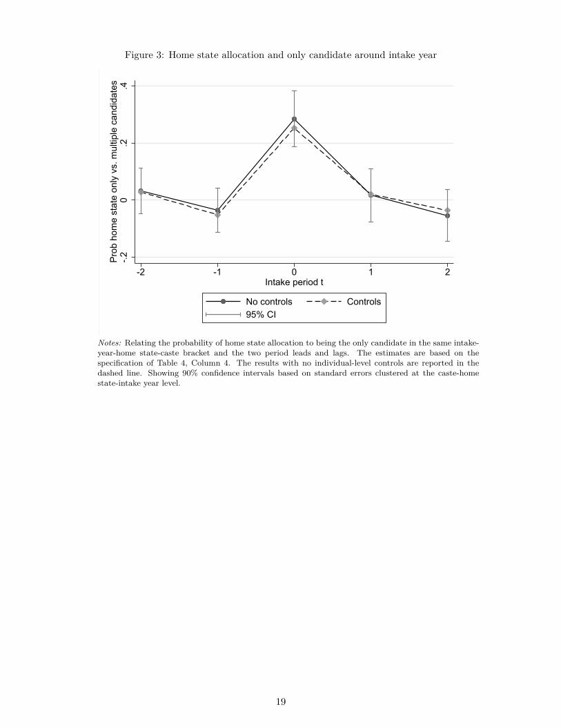
Figure 3: Home state allocation and only candidate around intake year

-.20

.2.4

Prob

hom

e st

ate

only

vs.

mul

tiple

can

dida

tes

-2 -1 0 1 2Intake period t

No controls Controls95% CI

Notes: Relating the probability of home state allocation to being the only candidate in the same intake-year-home state-caste bracket and the two period leads and lags. The estimates are based on thespecification of Table 4, Column 4. The results with no individual-level controls are reported in thedashed line. Showing 90% confidence intervals based on standard errors clustered at the caste-homestate-intake year level.

19

Figure 4: Home state allocation and ability to withstand illegitimate political pressure

-.15

-.1-.0

50

.05

.1W

ithst

andi

ng p

ress

ure

only

vs.

mul

tiple

can

dida

tes

-2 -1 0 1 2Intake period t

No controls Controls95% CI

Notes: Relating the ability to withstand illegitimate political pressure to being the only candidate inthe same intake-year-home state-caste bracket and the two period leads and lags. The estimates arebased on the specification of Table 6. The results with no individual-level controls are reported in thedashed line. Showing 90% confidence intervals based on standard errors clustered at the caste-homestate-intake year level.

20

Figure 5: Ability to withstand illegitimate political pressure and only candidate

Karn

atak

a

Biha

r

Guj

arat

Mad

hya

Prad

esh

Mah

aras

htra

Raj

asth

an

Har

yana

Oris

sa

Tam

il N

adu

Utta

r Pra

desh

Kera

la

Punj

ab Wes

t Ben

gal

Andh

ra P

rade

sh

-1.5

-1-.5

0.5

Impa

ct o

f onl

y ca

ndid

ate

on w

ithst

andi

ng p

oliti

cal p

ress

ure

Rank

Notes: Reduced form effect of only candidate on the ability to withstand illegitimate political pressure,separately estimated for each major state of India. Showing 90% confidence intervals based on standarderrors clustered at the caste-home state-intake year level.

21

Figure 6: Transfers per year and only candidate

0.2

.4.6

.81

Tran

sfer

s pe

r yea

r onl

y vs

. mul

tiple

can

dida

tes

4-8 9-12 13-15 16-24 25-29 >=30Years into IAS

Notes: Reduced form effect of only candidate on the number of transfers per year, separately estimatedfor tenure bins corresponding to the time-based promotion payscales. Showing 90% confidence intervalsbased on standard errors clustered at the caste-home state-intake year level.

22

Tables

Table 1: 360 performance scores by home state allocation

(1) (2) (3) (4) (5)Mean SD Ratings Officers Coverage

Effectiveness on the job 3.730 1.077 17,753 1,472 72.01%Probity of IAS officer 3.670 1.105 15,153 1,451 70.98%Withstanding illegitimate pressure 3.523 1.094 16,728 1,471 71.96%Sensitive towards poorer 3.527 1.141 17,047 1,471 71.96%Overall rating 3.646 1.057 17,698 1,472 72.01%

Notes: Performance scores for the cross-section of rated IAS officers in 2012-13. Reporting the descriptivestatistics (mean and standard deviation) for the subjective measures, where the scores range from 1(lowest) to 5 (highest). Column 3 and 4 report the total number of ratings and the total number of ratedofficers. Column 5 reports the coverage rate for the sample population of all active, centrally recruitedIAS officers with at least 8 years of tenure in 2012/13.

23

Table 2: IAS officer characteristics by home state allocation

(1) (2) (3) (4)Allocation Diff Home-Non-home

Means Home Non-Home Raw Within intakeUPSC Rank 44.483 56.091 -11.607*** -14.959***

(1.732) (1.791)Female 0.107 0.134 -0.027 -0.020

(0.017) (0.017)Urban 0.728 0.722 0.006 -0.002

(0.022) (0.023)Entry age 25.443 25.704 0.261** -0.022

(0.112) (0.108)Distinction 0.326 0.322 0.004 0.006

(0.024) (0.024)STEM 0.590 0.616 -0.025 -0.004

(0.025) (0.025)OBC 0.059 0.119 -0.059*** -0.024*

(0.015) (0.012)SC 0.168 0.116 0.052*** 0.061***

(0.017) (0.019)ST 0.078 0.059 0.019 0.022

(0.012) (0.014)Previous: Education/Research 0.173 0.147 0.026 -0.007

(0.018) (0.019)Previous: Finance/Banking 0.055 0.049 0.006 -0.002

(0.011) (0.012)Previous: None 0.294 0.299 0.005 0.010

(0.023) (0.023)Previous: Private/SOE 0.114 0.118 -0.003 0.008

(0.016) (0.017)Previous: Public 0.326 0.345 -0.018 0.003

(0.024) (0.025)Previous: Public - AIS 0.034 0.039 -0.005 -0.012

(0.009) (0.009)Cohort size 7.685 6.306 1.379*** 1.003***

(0.200) (0.388)Caste fractionalization 0.326 0.344 -0.017 0.025**

(0.011) (0.011)Intake year FEs - - - YDiff jointly zero: p-value 0.000*** 0.000***Observations 542 1326 1888 1888

Notes: Unit of observation is the IAS officer. Columns 1-2 show the mean characteristics for those whoreceived the home allocation and those who did not. Column 3 is the raw difference in means betweenhome and non-home allocated officers. Column 4 shows the mean difference among officers of the sameintake year. UPSC Rank is the entry exam (UPSC) rank in the intake year. Female is a dummy that is1 if the IAS officer is female. Urban is a dummy that is 1 if the IAS officer is from an urban background.Entry age is the age at which the IAS officer entered the IAS. Distinction is a dummy that is 1 if the IASofficer received an academic distinction. STEM is a dummy that is 1 if the IAS officer studied a STEMor Economics degree. Previous job: are categories for the previous positions the IAS officer held beforeentering IAS. OBC/SC/ST are dummies if the IAS officer is from Other Backward Castes, ScheduledCastes, Scheduled Tribes. Cohort size is the total number of officers allocated to same state in sameyear. Caste fractionalization is the fractionalization index for the cohort based on the caste categories.Robust standard errors. * p < 0.1, ** p < 0.05, *** p < 0.01.

24

Table 3: IAS officer characteristics by allocation bracket size (one vs. many candidates)

(1) (2) (3) (4)Candidates in bracket Diff Only-Many

Means Only (1) Many (>1) Raw Within bracketUPSC Rank 65.56 51.01 14.555*** -1.266

(2.401) (1.900)Female 0.185 0.119 0.066*** 0.074**

(0.022) (0.034)Urban 0.694 0.728 -0.034 0.039

(0.030) (0.038)Age at entry 26.446 25.512 0.933*** -0.087

(0.149) (0.199)Distinction 0.334 0.321 0.012 0.041

(0.032) (0.042)STEM 0.586 0.612 0.025 0.015

(0.033) (0.043)Previous: Education/Research 0.099 0.163 -0.064*** -0.012

(0.024) (0.028)Previous: Finance/Banking 0.041 0.052 -0.010 -0.017

(0.015) (0.020)Previous: None 0.305 0.297 0.008 0.002

(0.031) (0.041)Previous: Private/SOE 0.107 0.119 -0.011 -0.002

(0.022) (0.031)Previous: Public 0.417 0.328 0.088*** 0.002

(0.032) (0.045)Previous: Public - AIS 0.028 0.039 -0.010 0.026

(0.013) (0.017)Cohort size 5.355 7.100 -1.744*** 0.076

(0.274) (0.254)Caste fractionalization 0.425 0.329 0.096*** 0.003

(0.014) (0.017)Intake year FEs - - - YHome state-Caste FEs - - - YDiff jointly zero: p-value 0.000*** 0.556Observations 242 1646 1888 1880

Notes: Unit of observation is the IAS officer. Columns 1-2 show the mean characteristics for those whoare the only candidate in the intake year-home state-caste bracket. Column 3 is the raw difference inmeans between those who are only candidates and those with many candidates in the intake year-homestate-caste bracket. Column 4 shows the mean difference among officers of the same intake year andwithin the same home state-caste bracket. Rank is the overall rank in the intake year. Female is adummy that is 1 if the IAS officer is female. Urban is a dummy that is 1 if the IAS officer is froman urban background. Entry age is the age at which the IAS officer entered the IAS. Distinction is adummy that is 1 if the IAS officer received an academic distinction. STEM is a dummy that is 1 if theIAS officer studied a STEM or Economics degree. Previous job: are categories for the previous positionsthe IAS officer held before entering IAS. Cohort size is the total number of officers allocated to samestate in same year. Caste fractionalization is the fractionalization index for the cohort based on the castecategories. Robust standard errors. * p < 0.1, ** p < 0.05, *** p < 0.01.

25

Table 4: Predicting home state assignment with allocation rule

(1) (2) (3) (4)Allocated to home state

Mean of dep. var 0.276 0.276 0.276 0.285Only candidate 0.228*** 0.241*** 0.250*** 0.285***

(0.042) (0.046) (0.046) (0.050)Intake year FEs Y Y Y YHome state × Caste FEs Y Y Y YRank FEs - Y Y YIndividual controls - - Y YLeads and lags (2) - - - YObservations 1,880 1,868 1,868 1,700

Notes: Unit of observation is the IAS officer. Relating home state allocation to the instrument. Theinstrument only candidate is a dummy that is 1 if the IAS officer was the only candidate in the intakeyear-home state-caste bracket. Rank FEs are fixed effects for each rank in the entry exam. Individualcontrols are: age at entry, female dummy, a dummy for coming from an urban background, havingreceived an academic distinction, a STEM or Economics degree, dummies for previous job type. Robuststandard errors clustered at the caste-home state-intake year level. * p < 0.1, ** p < 0.05, *** p < 0.01.

26

Table 5: Social proximity and home state allocation

(1) (2)Distance home district Same language

Mean of dep. var 455.5 0.388Panel A: OLSHome state -482.150*** 0.692***

(16.116) (0.022)Panel B: IVHome state -495.720*** 0.829***

(87.548) (0.130)Kleibergen-Paap F -statistic 34.000 29.836Intake year FEs Y YHome state × Caste FEs Y YRank FEs Y YIndividual controls Y YObservations 1,625 1,868

Notes: Unit of observation is the IAS officer. Relating measures of social proximity to home stateallocation. Home state is a dummy that is 1 if the officer was allocated to his or her state of permanentdomicile. The instrument only candidate is a dummy that is 1 if the IAS officer was the only candidate inthe intake year-home state-caste bracket. Distance to home town is the distance (in miles) between theallocated state’s state capital and the officer’s home district. Same language is a dummy that is 1 if theIAS officer’s mother tongue is the first official language in the state. Rank FEs are fixed effects for eachrank in the entry exam. Individual controls are: age at entry, female dummy, a dummy for coming froman urban background, having received an academic distinction, a STEM or Economics degree, dummiesfor previous job type. Robust standard errors clustered at the caste-home state-intake year level. *p < 0.1, ** p < 0.05, *** p < 0.01.

27

Table 6: 360 performance ratings and home state allocation

(1) (2) (3) (4) (5)Effective Probity Pressure Pro-poor Overall

Mean of dep. var 3.730 3.671 3.524 3.528 3.647Panel A: OLSHome state 0.007 0.005 -0.001 0.020 0.050*

(0.026) (0.030) (0.026) (0.027) (0.029)Panel B: IVHome state -0.034 -0.202* -0.381*** -0.112 -0.103

(0.107) (0.119) (0.121) (0.113) (0.127)Kleibergen-Paap F -statistic 46.470 56.885 46.495 45.626 46.168Home state × Caste FEs Y Y Y Y YIntake year FEs Y Y Y Y YRespondent FEs Y Y Y Y YState × Tenure FEs Y Y Y Y YRank FEs Y Y Y Y YIndividual controls Y Y Y Y YObservations 17,744 15,128 16,712 17,037 17,689

Notes: Unit of observation is the score for a given IAS officer in 2012-13 with at least 8 years of tenure.Relating five measures of performance (effectiveness, probity, ability to withstand illegitimate politicalpressure, pro-poor orientedness and overall rating) to home state allocation. Home state is a dummythat is 1 if the IAS officer is allocated to his or her state of origin. Only candidate is a dummy that is 1 ifthe IAS officer was the only candidate in the intake year-home state-caste bracket. Panel A presents theOLS estimates. Panel B presents the IV results. Caste FEs are dummies for OBC, SC, ST. Individualcontrols are: rank FEs for each rank in the entry exam, age at entry, female dummy, a dummy forcoming from an urban background, having received an academic distinction, a STEM or Economicsdegree, dummies for previous job type. Standard errors clustered at the caste-home state-intake yearand individual IAS officer level. * p < 0.1, ** p < 0.05, *** p < 0.01.

28

Table 7: Withstanding pressure, home state allocation and state-level heterogeneity

(1) (2) (3)Withstanding pressure

Mean of dep. var 3.497 3.524 3.497Only candidate -0.142*** -0.138*** -0.142***

(0.041) (0.038) (0.041)× TI corruption index -0.110*** -0.117**

(0.036) (0.054)× Human Development Index 0.724** -0.087

(0.306) (0.451)Home state × Caste FEs Y Y YIntake year FEs Y Y YRespondent FEs Y Y YState × Tenure FEs Y Y YRank FEs Y Y YIndividual controls Y Y YObservations 15,644 16,712 15,644

Notes: Unit of observation is the IAS officer-year. Relating the ability to withstand illegitimate politicalpressure to home state allocation. Home state is a dummy that is 1 if the IAS officer is allocated tohis or her state of origin. The instrument only candidate is a dummy that is 1 if the IAS officer wasthe only candidate in the intake year-home state-caste bracket. TI corruption index is the state-levelTransparency International corruption index from 2005 as used by Fisman et al. (2014). The HDI is thestate-level Human Development Index in 2007. Caste FEs are dummies for OBC, SC, ST. Rank FEsare fixed effects for each rank in the entry exam. Individual controls are: age at entry, female dummy,a dummy for coming from an urban background, having received an academic distinction, a STEM orEconomics degree, having worked in education/research, private sector/SOE, public sector, public AIS.Standard errors clustered at the caste-home state-intake year and individual IAS officer. * p < 0.1, **p < 0.05, *** p < 0.01.

29

Table 8: Withstanding pressure, home state allocation and individual heterogeneity

(1) (2) (3) (4) (5) (6)Withstanding pressure

Mean of dep. var 3.524 3.524 3.524 3.524 3.524 3.524Only candidate -0.136*** -0.117*** -0.126*** -0.196*** -0.183*** -0.065

(0.038) (0.043) (0.040) (0.055) (0.062) (0.042)× Father ag/wage laborer -0.098

(0.074)× Father private sector -0.054

(0.080)× Father public sector 0.096

(0.066)× Urban background 0.062

(0.072)× UPSC test score 0.145***

(0.035)Home state × Caste FEs Y Y Y Y Y YIntake year FEs Y Y Y Y Y YRespondent FEs Y Y Y Y Y YState × Tenure FEs Y Y Y Y Y YRank FEs Y Y Y Y Y YIndividual controls Y Y Y Y Y YObservations 16,712 16,712 16,712 16,712 16,712 16,712

Notes: Unit of observation is the IAS officer-year. Relating the ability to withstand illegitimate politicalpressure to home state allocation. Home state is a dummy that is 1 if the IAS officer is allocated to hisor her state of origin. The instrument only candidate is a dummy that is 1 if the IAS officer was theonly candidate in the intake year-home state-caste bracket. Caste FEs are dummies for OBC, SC, ST.Rank FEs are fixed effects for each rank in the entry exam. Individual controls are: age at entry, femaledummy, a dummy for coming from an urban background, having received an academic distinction, aSTEM or Economics degree, having worked in education/research, private sector/SOE, public sector,public AIS. Standard errors clustered at the caste-home state-intake year and individual IAS officer. *p < 0.1, ** p < 0.05, *** p < 0.01.

30

Table 9: Posting type and home state allocation - Reduced form

(1) (2) (3) (4) (5) (6)Other state In Delhi Payscale Important Transfers Suspended

Mean of dep. var 0.0199 0.176 3.273 0.243 0.846 0.777Only candidate -0.007 -0.004 -0.005 -0.037** -0.021 -0.243***× 4-8 years (0.007) (0.008) (0.019) (0.015) (0.040) (0.074)Only candidate -0.027*** -0.053*** 0.010 -0.007 0.048 -0.480**× 9-12 years (0.009) (0.020) (0.025) (0.019) (0.049) (0.227)Only candidate -0.022* -0.101*** 0.140*** -0.006 0.140** 0.017× 13-15 years (0.013) (0.031) (0.040) (0.029) (0.063) (0.867)Only candidate -0.005 -0.036 0.063* -0.011 0.222*** -0.549× 16-24 years (0.011) (0.033) (0.035) (0.026) (0.074) (0.465)Only candidate -0.002 -0.152*** 0.067 -0.007 0.453*** -0.266× 25-29 years (0.011) (0.048) (0.071) (0.048) (0.142) (1.297)Only candidate -0.004 -0.287*** 0.239*** 0.034 0.530* 6.108× >= 30 years (0.009) (0.070) (0.091) (0.101) (0.288) (7.438)Individual FEs Y Y Y Y Y YYear FEs Y Y Y Y Y YTenure FEs Y Y Y Y Y YTest (p-value): all=0 0.011** 0.000*** 0.000*** 0.703 0.000*** 0.580Observations 41,677 41,677 41,676 41,677 41,677 41,677

Notes: Unit of observation is the IAS posting. Relating career outcomes to home state allocation. Otherstate is a dummy that is 1 if the officer is currently serving in another state. In Delhi is a dummy thatis 1 if the officer is serving in the Central Government. Payscale denotes the payscale of the IAS officer(1-7) in a given year. Important is the share of important positions held in a given year. Transfers isthe number of transfers in a given year. Suspended is a dummy that is 1 if the IAS officer is suspended(scaled × 100). Home state is a dummy that is 1 if the IAS officer is allocated to his or her state oforigin. The instrument only candidate is a dummy that is 1 if the IAS officer was the only candidatein the intake year-home state-caste bracket. Tenure FEs are fixed effects for each year of experience inthe IAS. Standard errors clustered at the caste-home state-intake year and individual IAS officer level.* p < 0.1, ** p < 0.05, *** p < 0.01.

31

Table 10: Board membership and home state allocation, by state

(1) (2) (3) (4) (5)Sits in # company boards in state Top 50%

Total Public Private firmMean of dep. var 0.0281 0.0281 0.0194 0.00765 0.0160Home state 0.152*** -0.221* -0.142* -0.078 -0.103*

(0.035) (0.121) (0.077) (0.053) (0.062)× Allocated home state 1.358*** 0.921*** 0.421** 0.693***

(0.446) (0.288) (0.200) (0.231)Kleibergen-Paap F -statistic - 47.494 47.494 47.494 47.494Individual FEs Y Y Y Y YState FEs Y Y Y Y YObservations 48,369 48,369 48,369 48,369 48,369

Notes: Unit of observation is the IAS officer-state pair. Sample of all IAS officers who entered between1975-2005. Relating membership in boards of companies in different states of India in 2018 to home stateallocation. Home state is a dummy that is 1 if the state is the IAS officer’s home state. Allocated homestate is a dummy that is 1 if the IAS officer was actually allocated to his/her home state. Columns 2-5report the instrumental variable estimates, where Home state × Allocated home state is instrumentedusing Home state × Only candidate. Member of company boards (#) is the number of boards in a statean IAS officer is member of, as registered by the Ministry of Corporate Affairs. Public/private breakdown the total number by whether firms are state-owned or private. Top 50% firm is the number offirms that are above median in terms of authorized capital. Standard errors clustered at the individualIAS officer level and the bilateral state × home state level. * p < 0.1, ** p < 0.05, *** p < 0.01.

32

A Appendix Figures

Figure A1: Determination of vacancies: Example 2006

Illustrating the assignment of categories (caste and home preference) to vacancies through the rosterrandomization for the year 2006. Vacancies are earmarked by caste status (O.B.C. denotes other back-ward castes, S.C./S.T. scheduled castes/tribes and unreserved the general castes) and home state (“I”denotes insider vacancies reserved for applicants from the same state; “O” denotes outsider vacanciesreserved for applicants from other states). The assignment occurs through a number line.

33

Figure A2: Assignment of categories (caste and home preference) to vacancies throughroster randomization

The final distribution of vacancies by state and caste/home quota for the year 2006. Vacancies areearmarked by caste status (O.B.C. denotes other backward castes, S.C./S.T. scheduled castes/tribesand unreserved the general castes) and home state (insider vacancies are reserved for applicants fromthe same state; outsider vacancies are reserved for applicants from other states).

34

Figure A3: Merit-based (UPSC rank) allocation based on caste and home preference match

Illustrating the ranking of candidates using the intake year of 2006. Candidates in a given year of intakeare ranked in descending order based on the UPSC entry exam score. Home state denotes the state fromwhich the candidate applied from. Category denotes the caste of the candidate, where O.B.C. denotesother backward castes, S.C. scheduled castes, S.T. scheduled tribes and General the unreserved castes.Whether home state opted denotes if the applicant indicated a preference to be allocated to the homestate.

35

Figure A4: Rotation of state groups over years

Division of state cadres into four groups and the rotation of groups in the order of IAS officer allocationover time, as illustrated by the group order in 2006. The groups of states rotate each year. In 2007, forexample, the order changes to Group II, Group III, Group IV, Group I.

36

Figure A5: Home state allocation and allocation bracket size: GEN

010

2030

400

1020

3040

010

2030

40

010

2030

40

0.2

.4.6

.81

0.2

.4.6

.81

0.2

.4.6

.81

0.2

.4.6

.81

1975 1985 1995 2005

1975 1985 1995 2005 1975 1985 1995 2005 1975 1985 1995 2005

Andhra Pradesh Bihar Gujarat Haryana

Himachal Pradesh Karnataka Kerala Madhya Pradesh

Maharashtra Orissa Punjab Rajasthan

Tamil Nadu Uttar Pradesh West Bengal

Share home allocations # candidates

Num

ber

Figure A6: Home state allocation and allocation bracket size: OBC

05

1015

05

1015

05

1015

05

1015

0.2

.4.6

.81

0.2

.4.6

.81

0.2

.4.6

.81

0.2

.4.6

.81

1975 1985 1995 2005

1975 1985 1995 2005 1975 1985 1995 2005 1975 1985 1995 2005






Num

ber

37

Figure A7: Home state allocation and allocation bracket size: SC

02

46

02

46

02

46

02

46

0.2

.4.6

.81

0.2

.4.6

.81

0.2

.4.6

.81

0.2

.4.6

.81

1975 1985 1995 2005

1975 1985 1995 2005 1975 1985 1995 2005 1975 1985 1995 2005






Num

ber

Figure A8: Home state allocation and allocation bracket size: ST

01

23

40

12

34

01

23

4

01

23

4

0.2

.4.6

.81

0.2

.4.6

.81

0.2

.4.6

.81

0.2

.4.6

.81

1975 1985 1995 2005

1975 1985 1995 2005 1975 1985 1995 2005 1975 1985 1995 2005






Num

ber

38

B Appendix Tables

39

Table B1: Share of home allocated and only candidates by home state × caste brackets

(1) (2) (3) (4) (5) (6) (7) (8) (9) (10) (11) (12)General caste Other Backward Castes Scheduled Castes Scheduled Tribes

Home state N Home Only N Home Only N Home Only N Home OnlyAndhra Pradesh 105 0.30 0.03 6 0.17 0.17 49 0.20 0.08 9 0.33 0.33Bihar 272 0.21 0.01 44 0.18 0.05 5 0.80 1.00 14 0.21 0.21Gujarat 11 0.64 0.73 0 0.00 0.00 5 0.40 0.60 0 0.00 0.00Haryana 67 0.27 0.04 4 0.00 1.00 17 0.47 0.53 0 0.00 0.00Himachal Pradesh 10 0.40 0.50 0 0.00 0.00 3 0.67 1.00 13 0.54 0.69Karnataka 36 0.50 0.36 11 0.09 0.27 11 0.18 0.27 9 0.33 0.78Kerala 48 0.46 0.10 11 0.18 0.45 2 0.50 0.50 0 0.00 0.00Madhya Pradesh 60 0.50 0.08 3 0.33 0.67 9 0.56 0.78 0 0.00 0.00Maharashtra 44 0.50 0.20 16 0.19 0.19 18 0.44 0.44 5 0.20 1.00Orissa 79 0.29 0.09 2 0.00 1.00 7 0.29 0.14 4 0.00 0.50Punjab 127 0.16 0.02 0 0.00 0.00 30 0.20 0.20 0 0.00 0.00Rajasthan 87 0.32 0.02 16 0.25 0.19 19 0.37 0.37 33 0.12 0.15Tamil Nadu 57 0.49 0.05 50 0.12 0.00 27 0.41 0.22 2 1.00 1.00Uttar Pradesh 397 0.20 0.00 25 0.20 0.08 32 0.47 0.31 3 0.00 1.00West Bengal 30 0.47 0.23 1 0.00 1.00 7 0.29 0.14 3 0.67 1.00

Notes: Reporting the total number of officers (N), the share of officers allocated to their home state (Home) and the share of only officers (Only) by the home state ×caste allocation brackets. Sample covers intake of all IAS officers between 1976-2005 from the 14 main states of India for which 360 performance scores were collected.

40

Table B2: 360 scores and home state allocation - linear IV

(1) (2) (3) (4) (5)Home state allocation=1

Mean of dep. var 0.363 0.365 0.359 0.359 0.362Panel A: First-stageOnly candidate -0.021*** -0.020*** -0.021*** -0.021*** -0.021***

(0.004) (0.004) (0.004) (0.004) (0.004)Panel B: 2SLS-IV

Effective Probity Pressure Pro-poor OverallMean of dep. var 3.730 3.671 3.524 3.528 3.647Home state 0.026 -0.366** -0.285** -0.157 -0.058

(0.117) (0.155) (0.134) (0.132) (0.132)Kleibergen-Paap F -statistic 32.896 29.771 33.430 33.076 32.709Home state × Caste FEs Y Y Y Y YIntake year FEs Y Y Y Y YRespondent FEs Y Y Y Y YState × Tenure FEs Y Y Y Y YRank FEs Y Y Y Y YIndividual controls Y Y Y Y YObservations 17,744 15,128 16,712 17,037 17,689

Notes: Unit of observation is the score for a given IAS officer in 2012-13 with at least 8 years of tenure.Relating five measures of performance (effectiveness, probity, ability to withstand illegitimate politicalpressure, pro-poor orientedness and overall rating) to home state allocation. Home state is a dummythat is 1 if the IAS officer is allocated to his or her state of origin. The instrument is the total numberof candidates in a given bracketintake year-home state-caste bracket. Caste FEs are dummies for OBC,SC, ST. Rank FEs are fixed effects for each rank in the entry exam. Individual controls are: age atentry, female dummy, a dummy for coming from an urban background, having received an academicdistinction, a STEM or Economics degree, a dummy for entering directly after completing education.Standard errors clustered at the caste-home state-intake year level and individual-level. * p < 0.1, **p < 0.05, *** p < 0.01.

41

Table B3: 360 performance ratings and home state allocation by stakeholder


Mean of dep. var 3.730 3.671 3.524 3.528 3.647Only candidate -0.118* -0.098 -0.207*** -0.056 -0.172***

(0.066) (0.069) (0.056) (0.064) (0.066)× State civil service 0.098 0.034 0.069 -0.099 0.135

(0.080) (0.088) (0.094) (0.080) (0.102)× Politicians (MLA) 0.163* -0.033 0.245*** 0.059 0.172*

(0.093) (0.116) (0.075) (0.116) (0.097)× Large firms 0.168** 0.056 0.064 0.062 0.220***

(0.078) (0.078) (0.070) (0.074) (0.070)× Media 0.162* -0.034 0.244*** 0.057 0.169*

(0.092) (0.116) (0.075) (0.116) (0.096)× NGO 0.108 0.044 0.090 0.025 0.220**

(0.085) (0.111) (0.095) (0.113) (0.098)Home state × Caste FEs Y Y Y Y YIntake year FEs Y Y Y Y YRespondent FEs Y Y Y Y YState × Tenure FEs Y Y Y Y YRank FEs Y Y Y Y YIndividual controls Y Y Y Y YStakeholder FEs Y Y Y Y YObservations 17,744 15,128 16,712 17,037 17,689

Notes: Unit of observation is the score for a given IAS officer in 2012-13 with at least 8 years of tenure.Relating five measures of performance (effectiveness, probity, ability to withstand illegitimate politicalpressure, pro-poor orientedness and overall rating) to home state allocation. Home state is a dummythat is 1 if the IAS officer is allocated to his or her state of origin. The instrument only candidate is adummy that is 1 if the IAS officer was the only candidate in the intake year-home state-caste bracket.Estimates are relative to assessments provided by IAS officers. Caste FEs are dummies for OBC, SC, ST.Rank FEs are fixed effects for each rank in the entry exam. Individual controls are: age at entry, femaledummy, a dummy for coming from an urban background, having received an academic distinction, aSTEM or Economics degree, a dummy for entering directly after completing education. Standard errorsclustered at the caste-home state-intake year level and individual-level. * p < 0.1, ** p < 0.05, ***p < 0.01.

42

Table B4: 360 performance ratings and home state allocation by info source


Mean of dep. var 3.730 3.671 3.524 3.528 3.647Only candidate 0.015 -0.068 -0.171** -0.043 -0.027

(0.053) (0.076) (0.072) (0.073) (0.066)× Network -0.055 -0.047 0.042 -0.013 -0.046

(0.065) (0.087) (0.082) (0.090) (0.072)× Media -0.025 0.002 0.039 0.009 -0.002

(0.054) (0.082) (0.073) (0.074) (0.066)Home state × Caste FEs Y Y Y Y YIntake year FEs Y Y Y Y YRespondent FEs Y Y Y Y YState × Tenure FEs Y Y Y Y YRank FEs Y Y Y Y YIndividual controls Y Y Y Y YStakeholder FEs Y Y Y Y YObservations 17,744 15,128 16,712 17,037 17,689

Notes: Unit of observation is the score for a given IAS officer in 2012-13 with at least 8 years of tenure.Relating five measures of performance (effectiveness, probity, ability to withstand illegitimate politicalpressure, pro-poor orientedness and overall rating) to home state allocation. Home state is a dummythat is 1 if the IAS officer is allocated to his or her state of origin. The instrument only candidate is adummy that is 1 if the IAS officer was the only candidate in the intake year-home state-caste bracket.Estimates are relative to assessments based on personally knowing the IAS officer. Network (Media) isa dummy that is 1 if the respondent knows the given officer through his/her social network (media).Caste FEs are dummies for OBC, SC, ST. Rank FEs are fixed effects for each rank in the entry exam.Individual controls are: age at entry, female dummy, a dummy for coming from an urban background,having received an academic distinction, a STEM or Economics degree, a dummy for entering directlyafter completing education. Standard errors clustered at the caste-home state-intake year level andindividual-level. * p < 0.1, ** p < 0.05, *** p < 0.01.

43

Table B5: Standard deviation of 360 performance ratings and home state allocation

(1) (2) (3) (4) (5)Standard deviation in residual 360 scores

Effective Probity Pressure Pro-poor OverallMean of dep. var 0.685 0.833 0.764 0.782 0.806Home state -0.194 -0.057 -0.147 -0.198 0.042

(0.190) (0.240) (0.209) (0.227) (0.217)Home state × Caste FEs Y Y Y Y YIntake year FEs Y Y Y Y YState × Tenure FEs Y Y Y Y YRank FEs Y Y Y Y YIndividual controls Y Y Y Y YStakeholder FEs Y Y Y Y YObservations 1,165 1,116 1,161 1,164 1,169

Notes: Unit of observation is the SD for scores given to an IAS officer in 2012-13 with at least 8 years oftenure. Relating the SD of all five measures of performance (effectiveness, probity, ability to withstandillegitimate political pressure, pro-poor orientedness and overall rating) to home state allocation. Thestandard deviation is calculated based on the 360 scores after partialling out respondent fixed effects.Home state is a dummy that is 1 if the IAS officer is allocated to his or her state of origin. The instrumentonly candidate is a dummy that is 1 if the IAS officer was the only candidate in the intake year-homestate-caste bracket. Estimates are relative to assessments based on personally knowing the IAS officer.Network (Media) is a dummy that is 1 if the respondent knows the given officer through his/her socialnetwork (media). Caste FEs are dummies for OBC, SC, ST. Rank FEs are fixed effects for each rankin the entry exam. Individual controls are: age at entry, female dummy, a dummy for coming from anurban background, having received an academic distinction, a STEM or Economics degree, a dummy forentering directly after completing education. Standard errors clustered at the caste-home state-intakeyear level and individual-level. * p < 0.1, ** p < 0.05, *** p < 0.01.

44

Table B6: Visibility of IAS officer and home state allocation, by stakeholder

(1) (2) (3) (4) (5) (6)Dummy=1 if IAS officer is known

Pooled Civil service MLA Firms Media NGOMean of dep. var 0.206 0.265 0.175 0.185 0.208 0.139IVHome state 0.004 -0.060 0.006 -0.028 0.047 0.125*

(0.044) (0.046) (0.075) (0.057) (0.072) (0.064)Kleibergen-Paap F -statistic 34.865 38.683 34.865 35.698 33.821 34.865Home state × State FEs Y Y Y Y Y YHome state × Caste FEs Y Y Y Y Y YIntake year FEs Y Y Y Y Y YState FEs × Tenure FEs Y Y Y Y Y YRank FEs Y Y Y Y Y YIndividual controls Y Y Y Y Y YObservations 89,723 29,617 15,060 14,839 15,147 15,060Notes: Unit of observation is the score for a given IAS officer in 2012-13 with at least 8 years of tenure.Relating five measures of performance (effectiveness, probity, ability to withstand illegitimate politicalpressure, pro-poor orientedness and overall rating) to home state allocation. Home state is a dummy thatis 1 if the IAS officer is allocated to his or her state of origin. Only candidate is a dummy that is 1 if theIAS officer was the only candidate in the intake year-home state-caste bracket. Caste FEs are dummiesfor OBC, SC, ST. Rank FEs are fixed effects for each rank in the entry exam. Individual controls are: ageat entry, female dummy, a dummy for coming from an urban background, having received an academicdistinction, a STEM or Economics degree, a dummy for entering directly after completing education.Standard errors clustered at the caste-home state-intake year level and individual-level. * p < 0.1, **p < 0.05, *** p < 0.01.

45

C Appendix Documentation

C.1 Converting unmatched insider allocations

In presence of open unreserved insider vacancies, the unreserved insider vacancy can beallocated to insider IAS officers from SC/ST and OBC (following the exact order) if there isan SC/ST (or OBC) outsider vacancy to allow for the exchange: For example, if Gujarat hasreceived two unreserved insider vacancies but only one Gujarati general caste to fill the firstslot, the second slot is opened to Gujarati SC/ST insiders, and if those are not available, toOBC insiders. The reallocation, however, is only permitted when there is a correspondingoutsider vacancy that can be converted to an unreserved outsider vacancy to maintain thequota among the caste vacancies. A Gujarati insider SC/ST then can only fill the unreservedinsider vacancy if a SC/ST outsider vacancy is available for exchange. Similar rules applyfor unfilled SC/ST or OBC insider vacancies. Open SC/ST insider vacancies that couldnot be filled are first relaxed to allow for OBC insider candidates and then to generalcandidates. Open OBC vacancies, similarly, can first be filled by SC/ST insider candidatesand then by general candidates (in both cases provided there is a corresponding outsiderslot for exchange). Any remaining open insider vacancies that could not be filled despitethe relaxation of the quotas are converted to outsider vacancies to ensure all vacancies arefilled.

C.2 Outsider allocation

The allocation of the outsiders and those who failed to be allocated to their preferred homestate (and are consequently converted to outsiders) is done according to a rotating rostersystem. The roster is created by arranging all 24 cadres in alphabetical order and dividingthem into four groups. These groups are devised on the basis of an average intake by eachgroup, which over a period of time is roughly equal:

1. Group I: Andhra Pradesh, Assam-Meghalaya, Bihar, Chhattisgarh and Gujarat

2. Group II: Haryana, Himachal Pradesh, Jammu & Kashmir, Jharkhand, Karnataka,Kerala and Madhya Pradesh

3. Group III: Maharashtra, Manipur-Tripura, Nagaland, Orissa, Punjab, Rajasthan andSikkim

4. Group IV: Tamil Nadu, AGMUT (UT Cadre), Uttaranchal, Uttar Pradesh and WestBengal

The outsider candidates are allocated in the order of merit across the four groups forthe outsider available vacancies (including those that have been converted from insidervacancies). In the first cycle, all candidates are allocated to their matching caste vacancyin the four states of Group I, starting with Andhra Pradesh. In the second cycle, theremaining candidates are allocated to their matching caste vacancies in Group II and so on.

46

Since states who receive officers earlier in the allocation process will receive higher rankedrecruits, the order of the groups shuffles each year to ensure that all states receive officersof comparable quality. In Appendix Figure A4, for example, Group III is the first group in2006, followed by Group IV, Group I and Group II. In the subsequent year, the groups willrotate and the allocation of outsiders will commence with Group II first, followed by GroupIII, Group IV and Group I.

47

social proximity and bureaucrat performance:...

Documents