serial data analysis tools - teledyne lecroy
TRANSCRIPT

Eye Doctor™ Serial Data Analysis Tools
Operator’s Manual July 2007

LeCroy Corporation
700 Chestnut Ridge Road Chestnut Ridge, NY 10977–6499 Tel: (845) 578 6020, Fax: (845) 578 5985
Internet: www.lecroy.com
© 2007 by LeCroy Corporation. All rights reserved.
LeCroy, ActiveDSO, WaveLink, JitterTrack, WavePro, WaveMaster, WaveSurfer, WaveExpert, WaveJet, and Waverunner are registered trademarks of LeCroy Corporation. Other product or brand names are trademarks or requested trademarks of their respective holders. Information in this publication supersedes all earlier versions. Specifications subject to change without notice.
Manufactured under an ISO 9000 Registered Quality Management System
Visit www.lecroy.com to view the certificate.
This electronic product is subject to disposal and recycling regulations that vary by country and region. Many countries prohibit the disposal of waste electronic equipment in standard waste receptacles.
For more information about proper disposal and recycling of your LeCroy product, please visit www.lecroy.com/recycle.
EYEDR-OM-E Rev A
915050-00 Rev A

Eye Doctor Operator’s Manual
EYEDR-OM-E Rev A 1
BLANK PAGE ........................................................................................................................... 2
INTRODUCTION........................................................................................................................ 3
VIRTUAL PROBING.................................................................................................................. 4 Eye Doctor Virtual Probe Option................................................................................................................................ 4 Configuration of Virtual Probing in the Processing Web: Introduction ....................................................................... 5 Virtual Probing Dialog ................................................................................................................................................ 7
System Description File ...................................................................................................................................... 7 Design and Implementation Rules...................................................................................................................... 8
Input/Output ............................................................................................................................................................. 11 Log ........................................................................................................................................................................... 12 Compile Button......................................................................................................................................................... 13 Configuration of Virtual Probing in the Processing Web: Details ............................................................................. 14 Helper Processors.................................................................................................................................................... 15
Reframer ........................................................................................................................................................... 15 Sparser ............................................................................................................................................................. 16 Interpolator........................................................................................................................................................ 17
System Description File Compiler............................................................................................................................ 18 File Overview .................................................................................................................................................... 18 Statements........................................................................................................................................................ 18 Defining a System............................................................................................................................................. 25 Log Messages................................................................................................................................................... 30 S-Parameter Files ............................................................................................................................................. 38 Mixed-mode S-parameters ............................................................................................................................... 39
System Descriptions ................................................................................................................................................ 42 Measurement Configuration ............................................................................................................................. 42 Output Configuration......................................................................................................................................... 46
EQUALIZER EMULATION ...................................................................................................... 52 Eye Doctor Equalization Option ............................................................................................................................... 52 Configuration of Equalizer Emulation in the Processing Web ................................................................................. 52
Basic Equalized Receiver Configuration .......................................................................................................... 57 Feed Forward Equalizer (FFE) Configuration................................................................................................... 59 Decision Feedback Equalizer (DFE) Configuration .......................................................................................... 60
Connection of the Equalized Receiver..................................................................................................................... 61 Equalized Receiver Example ................................................................................................................................... 62

Eye Doctor
2 EYEDR-OM-E Rev A
BLANK PAGE

Eye Doctor Operator’s Manual
EYEDR-OM-E Rev A 3
Introduction Eye Doctor is a software tool that operates inside of LeCroy oscilloscopes. The tool consists of two major features:
• Virtual Probing (enabled by the EYEDR_VP option).
• Ideal Equalizer Emulation (enabled by the EYEDR_EQ option).
The Virtual Probing feature enables a variety of advantages in signal probing situations including:
• the ability to compensate for probe loading effects by allowing you to see waveforms that occur in a circuit as they would with and without the probe connected to it.
• the ability to acquire waveforms that occur in locations other than the probing point.
• the ability to acquire waveforms that would occur in circuit configurations different from the configuration actually used for the measurement.
The Ideal Equalizer Emulation feature enables the emulation of various equalizer configurations including:
• linear transversal, tapped delay line, and linear feed-forward equalizers.
• clock recovery.
• decision feedback equalization (DFE).
The equalizer emulation feature allows you to see the recovered data, clock, and equalized waveform. The equalizers can be specified by tap delay, number of taps, and tap coefficients, or the equalizers can be automatically trained to optimize settings, utilizing blind adaptation.

Eye Doctor
4 EYEDR-OM-E Rev A
Virtual Probing In order to use the virtual probing feature, you should verify that you have at least one of the following requirements:
• the need to compensate for probe effects, both loading and through response.
• the need to see probed waveforms as if the probe were not connected to the circuit.
• the need to see waveforms at locations in a circuit other than the probing location.
• the need to see waveforms in circuit configurations other than the circuit configuration in which the measurement is taking place.
If you have these requirements, the virtual probing feature will come in handy. In order to use virtual probing, you will need the following:
• an accurate and complete description of the circuit configuration, both in the probing configuration and the configuration in which you want to see the virtual waveforms.
• accurate and complete measurements, models, or assumptions about the behavior of the various circuit components in the system, including the probing elements and the oscilloscope.
You will provide this information to the oscilloscope through two key types of files:
• system description file – a file that describes the various circuit descriptions to the oscilloscope.
• S-parameter files – Touchstone format files that describe, through S-parameters, the behavior of the circuit components.
Of course, you will also need the EYEDR_VP option installed on your oscilloscope.
The following sections step you through basic usage of virtual probing, followed by details of operation.
Eye Doctor Virtual Probe Option The Eye Doctor Virtual Probe option might already be loaded on your oscilloscope. Go to Help – About to show the dialog that contains the list of software options. If the list includes the option code EYEDR_VP, then your oscilloscope has already been outfitted with the Eye Doctor Virtual Probe option. If not, then installation of the option is accomplished and verified through the Utilities menu. The option requires a unique option key.
In order to obtain the option key for the EYEDR_VP option, you must provide the oscilloscope ID and the Serial # of the oscilloscope to LeCroy. LeCroy will then provide an option key consisting of 16 hexadecimal digits for entry. Correct installation of the key is indicated by the presence of the EYEDR_VP option under “Installed Option Keys.”

Eye Doctor Operator’s Manual
EYEDR-OM-E Rev A 5
In addition to the option key, your oscilloscope must have firmware version 5.0.4 or higher. Your current firmware version can be found on the Status tab of the Utilities Setup dialog.
The EYEDR_VP option enables the virtual probing features, along with the processing web editor. The processing web editor allows editing of processing configurations through a unique graphical user interface.
Configuration of Virtual Probing in the Processing Web: Introduction The processing web editor is accessed through the Math Setup menu.
The Math main dialog indicates how the math functions are defined, and provides tabs for each of the definable math functions. Selecting any math function tab allows you to configure a math function.
Along the left side of each math setup dialog there are four options for math function configuration. These are single, dual, graph, and web edit. Web edit is only available with the web editing option (enabled by the EYEDR option, as well as with the XWEB option). When web edit is selected, the processing web can be accessed through the Show Processing Web button.
When the processing web opens, you will find all possible waveform sources on the left and all possible waveform outputs on the right. In this case, F1, F2, F3, and F4 are defined as processing web edit waveforms, so icons for these functions are shown in the Web Editor. Functions that are not defined as “web edit” are not shown.

Eye Doctor
6 EYEDR-OM-E Rev A
To access the Eye Doctor components, select the Add Math button. This displays a dialog containing all math functions available on your oscilloscope. Select the Eye Doctor category to display all of the Eye Doctor math functions. When used within the web editor, these functions are referred to as processors.
Select VirtualProbe for the Virtual Probing component. The Virtual Probing component (an eight-input, eight-output processor) appears in the processing web. A dialog in the lower right corner allows access to the internal configuration dialog by means of the Settings button.

Eye Doctor Operator’s Manual
EYEDR-OM-E Rev A 7
Virtual Probing Dialog
The Virtual Probing dialog has several sections:
1. System Description File Designation.
2. Design and Implementation Rules.
3. Input/Output.
4. View Log Button.
5. Compile Button. System Description File
This entry box allows selection of the text file used to provide a system description. This file and file format will be described below in great detail. Accompanied by reference S-parameter data, this file provides the complete circuit description and behavior in the desired configuration for the virtual probing system. Also, it will reference measurement (input) nodes and output nodes of the circuit.

Eye Doctor
8 EYEDR-OM-E Rev A
Design and Implementation Rules
The design and implementation rules that govern the behavior of the system include
• min and max sample rate for which virtual probing is allowed, along with the intended sample rate
• time length
• filter die down amounts
• measurement filter bandwidth and order
In operation, the sample rate is derived from the sample rate of the waveform connected to the first input pin of the processing component (labeled In0). Until the component is hooked up, and actual waveforms are being processed, it is helpful to provide the intended system sample rate so that the system can be preconfigured. You do this by specifying the sample rate. However, this number may change when the component is processing actual waveforms; i.e., the system will adapt to changing sample rates during operation.
Some sample rates, on the other hand, simply do not make sense for component operation. For example, if you have S-parameter data going out to 20 GHz intended for virtual probing of a 10 Gb/s serial data system, it will not make sense for this component to operate below 40 GS/s. This is because a 40 GS/s sample rate dictates a 20 GHz Nyquist rate. So, the min sample rate is set to 40 GHz to handle changes in oscilloscope sample rate. Furthermore, there may be situations where maximum sample rates are undesirable, as well. Bracket the intended sample rate with the min and max. If the system is designed to operate at only one sample rate, set the min, max, and intended sample rate to the same value.
The Time Length is used to control the internal frequency resolution and absolute maximum impulse response length. The Filter Die Down amount is utilized to truncate the impulse response from the maximum amount governed by the time length to a smaller length that includes only the portion of the impulse response actually needed for reasonable accuracy, and to create impulse responses with proper cause and effect relationships.
The Measurement Bandwidth and Filter Order are used to control the bandwidth and filter order of a filter applied to account for the bandwidth of the oscilloscope and probing system.
Time Length
The time length defines the absolute maximum size of the impulse response, and therefore the internal frequency resolution. All S-parameter data is internally interpolated to match a frequency resolution capable of creating impulse responses with the desired maximum length.
The maximum impulse response length is important for two reasons. One is that, in some systems with long cables or backplanes, reflections and the effects of reflections take a long time to propagate. The virtual probing feature has no knowledge of these propagation times, since system behavior is provided as S-parameter data. Therefore, you must provide a number that is appropriate for your system. Usually, this number is at least four or five times the propagation time from a transmitter source to either the oscilloscope input or the receiver in the system, whichever is larger. If reflections are not large, this number can be made smaller. Generally, aside from system compilation time, this number can be safely made rather large (therefore defaulting to 20 ns).
The time length must also be made large enough to retain proper cause and effect relationships. This is because the virtual probing component utilizes FFT methods to determine system impulse responses. FFT methods suffer from the fact that when you take the inverse FFT (to create a finite impulse response — FIR — filter), there are sometimes causality issues, since the impulse response is actually the response to a train of pulses. Sometimes, bumps in the impulse response appear earlier in time than the response when, in fact, they are due to effects that occur after the response. Making the time duration large helps to eliminate these possibilities by setting the space between impulses in the impulse train far apart, thereby allowing large time separation between the impulse responses.

Eye Doctor Operator’s Manual
EYEDR-OM-E Rev A 9
Example of wrong cause/effect relationship
Example of correct cause/effect relationship
Filter Die Down
The Filter Die Down defines the length of the impulse response. The length of the impulse response extends from time zero to the last time that the magnitude of the response dips below this value. It is used to:
• limit the impulse response to a length that can reduce computation by not considering unimportant bumps in the response.
• reduce cause and effect relationship problems.
Since the height of an impulse response varies with sample rate, the amount specified is normalized to a particular sample rate: 20 GS/s. This means that if the actual sample rate utilized were, for example, 200 GS/s, the die down amount actually used internally will be 1/10th of the number specified.
The die down amount calculated internally is used as a threshold value. Internally, after a filter impulse response is generated, the system scans backward and forward in time starting at time zero and retains the impulse response from time zero out to the last point that is above this threshold.
Take the impulse responses shown in Figure 1and Figure 2 below. Figure 1, is a system with a time length of 20 ns, and a die down amount of 0.001. In this case, the major bumps end around 5 ns, but the portion all the way out to 18 ns is included. Utilization of this impulse response requires a filter that is almost 400 taps long. Also, while not happening in this case, the last bumps that occur at 18 ns could actually be occurring prior to the main bump starting at -2 ns.

Eye Doctor
10 EYEDR-OM-E Rev A
2 0 2 4 6 8 10 12 14 16 180.05
0
0.05
0.1
0.15
. Figure 1 – Virtual Probe Impulse Response (0.001 Filter Die Down Amount)
In the impulse response shown in Figure 2, the die down amount is set at 0.003. Notice that the impulse response has been shortened to around 5 ns (about 120 taps). There is no real loss of accuracy, since the portion from 5 to 18 ns is not overly significant. Furthermore, it is more likely that this impulse response represents a proper cause and effect relationship.
2 0 2 4 6 8 10 12 14 16 180.05
0
0.05
0.1
0.15
. Figure 2 – Virtual Probe Impulse Response (0.003 Filter Die Down Amount)
Measurement Bandwidth and Filter Order
In the process of calculating internal filters for virtual probing, the possibility exists for filters that produce excessive amounts of boost especially at high frequencies. Often, this is due to the fact that the oscilloscope channel or probing element has limited bandwidth and filter calculations extend to high frequencies. Said more generally, whenever the path from the transmitter to the oscilloscope channel contains more high frequency attenuation (less bandwidth) than the path to the virtual probing points, internal filters generated for virtual probing will tend to contain unintended high frequency boost.
Since the purpose of virtual probing is not to extend bandwidth, entering the aggregate probe and oscilloscope channel bandwidth can mitigate these effects.
In addition to oscilloscope and probe effects, often models provided for devices have limited bandwidth, as well, and are often measured with less high frequency accuracy. In these cases, it is useful to enter a number for the measurement bandwidth that reflects the accuracy of high frequencies. In other words, the measurement bandwidth should be set appropriately for the bandwidth of various system components.
The filter utilized for handling the measurement bandwidth is generally a high order filter. It is implemented as a filter that has a magnitude response given by a Butterworth filter of a given order. The phase response is always

Eye Doctor Operator’s Manual
EYEDR-OM-E Rev A 11
linear. The default value is 20, which is a very high order filter, but for sharper cutoff, higher orders can be used. A filter rolls off at 20 dB/decade (or 6 dB/octave) more for every increase in filter order.
Input/Output The Input/Output box contains the Input Pin Assignments and Output Pin Assignments. These Pin assignments are the names of the voltage nodes described in the system description file assigned to the input and output pins of the component. The boxes in the dialog are read-only and are filled in after successful compilation of the system description file specified.
Since the pin assignments depend on the system description file, the names are not known until the system description file is compiled — when the file is compiled, these names are filled in, directing you to ensure that the correct connections are made.
For example, if a system description file described measurement nodes labeled sc1 and sc2 (corresponding, for example, to oscilloscope channels 1 and 2) and the output nodes were labeled lpe and lme, then the Input/Output box might show the following after compilation:
These pin assignments dictate the following connections for the component:
Note that the eight input and output pin assignments reflect the eight input and output pins. In practice, usually only a small number of either is actually used.

Eye Doctor
12 EYEDR-OM-E Rev A
Log During compilation of the system description file, there are many things that need to go right in order for the system to properly operate. In order to see the compilation status, a log is provided. An example is shown below:

Eye Doctor Operator’s Manual
EYEDR-OM-E Rev A 13
The log shows the compilation progress in reverse order; the top line is the last message logged. The log can be exported to a text file and cleared. The complete log listing from the text file is shown next:
0 11.20.2006 17:03:05 Informational File: C:\NetList.txt (null)
1 11.20.2006 17:03:05 Informational Devices Counted: 8 (null)
2 11.20.2006 17:03:05 Informational Nodes Counted: 8 (null)
3 11.20.2006 17:03:20 Informational 8 Devices Assigned (null)
4 11.20.2006 17:03:20 Informational 8 Nodes Assigned (null)
5 11.20.2006 17:03:20 Informational Device Connections and Nodes Verified (null)
6 11.20.2006 17:03:20 Informational 4 Stimuli Assigned (null)
7 11.20.2006 17:03:20 Informational System Defined (null)
8 11.20.2006 17:03:20 Informational Measures Counted: 2 (null)
9 11.20.2006 17:03:20 Informational Outputs Counted: 2 (null)
10 11.20.2006 17:03:20 Informational Degrees of Freedom Specified: 2 (null)
11 11.20.2006 17:03:20 Informational With Respect to 4 Stimuli Specified (null)
12 11.20.2006 17:03:20 Informational Measures, Outputs and StimDefs Assigned (null)
13 11.20.2006 17:03:20 Informational Stimulus and Node Vector Built (null)
14 11.20.2006 17:03:21 Informational System Characteristics Matrix Built and Inverted (null)
15 11.20.2006 17:03:21 Informational System Characteristics Matrix and Stimuli Vector Reduced(null)
16 11.20.2006 17:03:21 Informational Node Voltage Vector Built (null)
17 11.20.2006 17:03:21 Informational Voltage Extraction Matrix Built (null)
18 11.20.2006 17:03:21 Informational Writing Filters (null)
19 11.20.2006 17:03:21 Informational Filter: Filter_lpe_DueTo_sc1_20p0.txt (null)
20 11.20.2006 17:03:21 Informational Filter: Filter_lpe_DueTo_sc2_20p0.txt (null)
21 11.20.2006 17:03:21 Informational Filter: Filter_lme_DueTo_sc1_20p0.txt (null)
22 11.20.2006 17:03:21 Informational Filter: Filter_lme_DueTo_sc2_20p0.txt (null)
23 11.20.2006 17:03:21 Informational Reading Filters (null)
24 11.20.2006 17:03:21 Informational Output Selection: lpe (null)
25 11.20.2006 17:03:21 Informational Filter: Filter_lpe_DueTo_sc1_20p0.txt (null)
26 11.20.2006 17:03:21 Informational Filter: Filter_lpe_DueTo_sc2_20p0.txt (null)
27 11.20.2006 17:03:21 Informational Output Selection: lme (null)
28 11.20.2006 17:03:21 Informational Filter: Filter_lme_DueTo_sc1_20p0.txt (null)
29 11.20.2006 17:03:21 Informational Filter: Filter_lme_DueTo_sc2_20p0.txt (null)
The log and log file contain messages that are informational, warnings, or errors. If a compilation succeeds, the log contains only informational messages. If the compilation fails, it will show one or more errors. The log file contains descriptions of all log messages and their meaning to help you debug problems with the system description files.
Compile Button The compile button is used to force system file compilation prior to the processing of waveforms. It is useful because you will need to compile the file in order to see the input and output pin assignment names prior to hooking up the component. Also, it is more expedient to deal with compilation errors prior to actually running the component in the system, where it becomes more difficult to control the oscilloscope due to waveform processing.

Eye Doctor
14 EYEDR-OM-E Rev A
Configuration of Virtual Probing in the Processing Web: Details Once the component has been placed in the processing web, the next steps are to:
1. edit and select the system description file.
2. set the min, max, and intended sample rates, making sure that the intended sample rate is within the min and max specified.
3. select the time length and filter die down value.
4. open the log.
5. compile the system.
6. review the log and ensure that the compilation is successful. If unsuccessful, repeatedly modify the system description file, clear the log, and recompile until the compilation is successful.
7. examine the input and output pin assignments.
8. connect the component pins appropriately in the processing web by connecting the appropriate channel and math inputs and outputs to the component.
9. set the oscilloscope to the correct sample rate.
10. trigger the oscilloscope, allowing waveforms to be produced and processed.
Connection of component pins is done by selecting a pin and dragging to the desired connection point.
As an example, suppose a system description file described measurement nodes labeled sc1 and sc2 (corresponding, for example, to oscilloscope channels 1 and 2) and the output nodes were labeled lpe and lme, for positive and negative voltages at a load, respectively. Suppose further that we are interested in the differential voltage developed at the load. A system might be connected as follows:
Here, oscilloscope channels 1 and 2 are connected to input pins 0 and 1, respectively. Furthermore, a difference component (one that takes the difference of two waveforms) is connected to output pins Out0 and Out1. The output of the difference component is connected to a reframer component, and the output of the reframer (see the Reframer, section of the manual) is connected to F1, indicating that math function F1 now produces the waveform

Eye Doctor Operator’s Manual
EYEDR-OM-E Rev A 15
corresponding to the differential voltage at the load by processing the waveforms acquired on oscilloscope channels 1 and 2.
(The Reframer component is explained in the Helper Processors section of this chapter.)
Once F1 is turned on by selecting Math Setup… from the menu bar, and the oscilloscope is triggered, you will see your waveforms, as shown below:
Note that there will be gaps in the waveform, usually on both the right and left portions of the screen. This is due to the fact that the filter that produces these waveforms requires startup samples for the FIR filter employed, and because the waveforms provided by the virtual probing component are either delayed or advanced in time. These gaps can be removed by zooming the waveform horizontally. Shown above is the virtually probed differential waveform at the receiver due to a 10 Gb/s signal probed at the transmitter.
Helper Processors There are several helper processors that help in dealing with floating point waveforms and with sample rates. These are:
• Reframer – handles upper and lower bounds on floating point waveforms for display and downstream processing.
• Sparser – lowers the sample rate of (decimates) a waveform.
• Interpolator – increases the sample rate of (upsamples) a waveform. Reframer
The reframer handles vertical reframing of floating point waveforms, meaning it handles how the waveform will be interpreted when it needs to be displayed on the screen, or when it needs to be converted into fixed point format for fixed point waveform processors. In essence, it sets a good upper and lower extent for the waveform.
The controls on the dialog consist of the following possibilities:
• Fit Every Time – a new frame is determined for every new waveform. This is very slow because it requires all of the data points from the input waveform – something you want to avoid.

Eye Doctor
16 EYEDR-OM-E Rev A
• Fit Frame To Data Once – allows you to set the frame once a waveform has been acquired and to keep it that way forever after – this is the most useful situation. Once you have waveforms available in the system and you know the sizes, you press this button and it determines the frame from the waveforms.
• Using Region – this allows you to center the waveform in the entire screen (All) or the lower or upper half of the screen. All is recommended.
• One Click Larger – the vertical frame is set so that the waveform fills the entire extent of the frame (to the next highest 1, 2, 5 sequence of vertical scale). If you think the waveform might still go outside these extents based on the use of the Fit Frame To Data Once button, you can set this to one click larger to make the frame a little bigger to handle these possibilities.
In the Eye Doctor System, a reframer should be placed on the output of any component that produces floating point waveforms. These are identified with turquoise colored output pins (as on the Virtual Probe component) as opposed to blue pins which are integer waveforms. Sparser
The sparser is a component that downsamples a waveform. In general, this is not necessary as you will tend to acquire waveforms at the appropriate sample rates, but sometimes it is useful to lower the sample rate of a waveform to either increase the speed of processing or to reduce excessively large sample rates that can appear especially when Eye Doctor is used with the LeCroy WaveExpert series of oscilloscopes. For example, a WaveExpert can generate waveforms with, for example, 512 points per unit interval. When this is performed on a 6 Gb/s waveform, for example, it produces a waveform with a sample rate of just over 3 TS/s. This is overkill for processing and may produce many problems, with speed of processing being perhaps the most obvious one.
The Virtual Probing component is restricted to a maximum sample rate of 500 GS/s, which is still usually overkill. For a 6 Gb/s waveform, it is usually not necessary to sample in excess of approximately 40 GS/s. This means that on a WaveExpert, you can usually safely sample at about 8 samples per UI. This would be recommended for processing. If you have a waveform that has already been acquired at extremely high sample rates, you can place sparsing components on the waveform to decrease the sample rate by throwing away samples.

Eye Doctor Operator’s Manual
EYEDR-OM-E Rev A 17
The sparser dialog has two controls:
• Sparsing factor – the factor by which to reduce the sample rate.
• Sparsing offset – the sample point offset of the waveform to begin sparsing.
Leave sparsing offset at zero and set the sparsing factor to the amount by which you want to reduce the sample rate. In the above example, where a 6 Gb/s waveform was acquired with 512 points per UI, set the sparsing factor to 76 to reduce the sample rate to around 40 GS/s. Of course, when you do this, you will need to ensure that aliasing does not occur. Aliasing occurs if there is signal content present above ½ the resulting sample rate (above 20 GHz in this case). Interpolator
The interpolator increases the sample rate of a waveform. It does so by interpolating new points. Interpolation is always valid when there is no aliasing (i.e., all of the original waveform content appears lower than ½ the sample rate of the waveform). Interpolation is useful in Eye Doctor to produce waveforms that are smoother and make better looking eye patterns.
The Interpolator has several controls:
• Linear, Cubic, SinX/X – controls how the interpolation is performed. Use SinX/X.
• Upsample by – controls the upsample factor, which is the amount by which the sample rate is to be increased.

Eye Doctor
18 EYEDR-OM-E Rev A
• Only by 2, 5… - controls the granularity of the Upsample by control. Generally, only numbers in a 1, 2, 5 sequence can be selected like 2, 5, 10, 20, 50, 100, etc. Checking this box allows any integer number to be selected.
System Description File Compiler File Overview
A system description file is a text file that describes the system. Only lines in the file that begin with a period are considered to contain a valid statement. Lines that do not begin with a period are simply ignored and can be used for comments.
All statements begin with a period. They are:
• .Device – Declares a device, a device name, the number of ports, and its behavior (i.e., what its S-parameters are).
• .Node – Declares a voltage node, a name, and two ports of two devices associated with the node. It defines a port-to-port connection between two devices.
• .Stim – Declares a stimulus and the device and port from the origin of the stimulus.
• .Meas – Declares a voltage measurement node. It defines the voltage nodes on which the resultant filters will operate.
• .Output – Declares a voltage output node. It defines the voltage nodes that the resultant filters will produce.
• .StimDef – Declares new stimuli and the relationship of these new stimuli to the stimuli declared through the .Stim statement.
Statements
.Device
The device statement is used to declare the devices in your system. A device is considered as a circuit element (defined with S-parameters) with a name and a given number of ports.
.Device [Name] [NumPorts] [Type]
[Name] is an alphanumeric string and must be unique for each device declared in the system.
[NumPorts] is the number of ports in the device.
[Type] is the type of device and can be one of the following keywords:
• File.
• IdealThru.
• IdealTermination.
• IdealOpen.
• IdealShort.
• IdealPowerSplitter.
• SingleEndedToMixedModeConverter.
• R.
• L.
• C.
File is the only device type that utilizes an S-parameter file. For system components that are assumed ideal, you can use the ideal types (with loss of accuracy if the components do not actually match these ideal types). Some ideal types, like the IdealTee should truly be used as ideal types (the tee, for example, connects multiple device ports together and is truly ideal). The S-parameter file is the common interface for both measured and modeled

Eye Doctor Operator’s Manual
EYEDR-OM-E Rev A 19
devices. If you take VNA or TDNA measurements of devices, you simply export these as Touchstone format S-parameter files and declare them here. Similarly, if you have models of devices from microwave simulators or electromagnetic system solvers, you would similarly export the S-parameter files in Touchstone format and use them here. Almost all microwave modeling and simulation packages have this export capability.
File
The device type File instructs the system to get the S-parameters for the device from a file, whose name directly follows the word file in the device declaration.
The file name must be delimited by double quotes.
The extension of the file must be .s[NumPorts]p, and must reflect an S-parameter file with the same number of ports as specified in the device declaration.
An example is
.Device transmissionLine 4 file "tline.s4p"
where, in this example, the device is named transmissionLine, has four ports, and has S-parameters that come from the file named tline.s4p. Note that the 4 in the file extension matches the number of ports declared.
S-parameter file paths are always assumed relative to the path containing the system description file. In other words, if declared as a file name only, they refer to files contained in the same directory as the system description file. This allows designs to be kept in a directory together with the S-parameter files that are easily relocated on the disk.
IdealThru
The device type IdealThru instructs the system to use a model of an ideal thru for the device. An ideal thru must have an even number of ports, with the first half considered as the input ports and the second half considered as the output ports. The ideal thru has a reflection coefficient of zero at all ports, and directly connects to one other port and is isolated from all other ports.
An example is
.Device transmissionLine 4 IdealThru
This example would create a four-port section called transmissionLine. The section would have S-parameters of
⎥⎥⎥⎥
⎦
⎤
⎢⎢⎢⎢
⎣
⎡
=
0010000110000100
S
which means that signals pass from port 1 to 3 and 3 to 1 uniquely with no return loss and no interaction. Similarly, signals pass from port 2 to 4 and 4 to 2 uniquely with no return loss.
IdealTermination
The device type IdealTermination instructs the system to use a model of an ideal, perfect termination. The S-parameters of an ideal termination are zero everywhere.
An example is
.Device termination 2 IdealTermination
This example would create a two-port section called termination. The section would have S-parameters of zero everywhere.
IdealShort
The device type IdealShort instructs the system to use a model of an ideal, perfect short. The S-parameters of an ideal short are zero everywhere, except the reflection coefficient of the port, which is -1.
A P-port ideal short has S-parameters of:

Eye Doctor
20 EYEDR-OM-E Rev A
⎥⎥⎥⎥
⎦
⎤
⎢⎢⎢⎢
⎣
⎡
−
−−
=
1...00............0...100...01
S
An example is:
.Device termination 1 IdealShort
This example would create a one-port section called termination. The section would have S-parameters of:
[ ]1−=S
IdealOpen
The device type IdealOpen instructs the system to use a model of an ideal, perfect open. The S-parameters of an ideal open are zero everywhere, except the reflection coefficient of the port, which is 1.
A P-port ideal open has S-parameters of:
⎥⎥⎥⎥
⎦
⎤
⎢⎢⎢⎢
⎣
⎡
=
1...00............0...100...01
S
An example is:
.Device termination 2 IdealOpen
This example would create a two-port section called termination. The section would have S-parameters of:
⎥⎦
⎤⎢⎣
⎡=
1001
S
IdealPowerSplitter
The device type IdealPowerSplitter instructs the system to use a model of an ideal, perfect resistive power splitter. An ideal resistive power splitter is a device that presents a perfect match to an input at all ports, and transfers power evenly from one port to all others. The device is symmetric.
A P-port ideal power splitter has S-parameters of:
⎥⎥⎥⎥⎥⎥⎥
⎦
⎤
⎢⎢⎢⎢⎢⎢⎢
⎣
⎡
−−
−−
−−
=
0...1
11
1............
11...0
11
11...
110
PP
PP
PP
S
An example is:
.Device split0 3 IdealPowerSplitter
This would declare a device named split0 with 3 ports, having S-parameters given by:
⎥⎥⎥
⎦
⎤
⎢⎢⎢
⎣
⎡=
011101110
21S

Eye Doctor Operator’s Manual
EYEDR-OM-E Rev A 21
SingleEndedToMixedModeConverter
The device type SingleEndedToMixedModeConverter instructs the system to use a model of a device that converts single-ended signals into mixed-mode signals. It is a device that has exactly four ports. Ports 1 and 2 are single-ended. Ports 3 and 4 are differential and common-mode, respectively.
A SingleEndedToMixedModeConverter has the following S-parameters:
⎥⎥⎥⎥
⎦
⎤
⎢⎢⎢⎢
⎣
⎡
−−
⋅=
0011001111001100
21S
An example is:
.Device modeconv 4 SingleEndedToMixedModeConverter
This would declare a SingleEndedToMixedModeConverter named modeconv.
Note that this component has several key uses. One is that it can be used to interface to devices with mixed-mode S-parameters provided. Another is that it can be used to convert mixed-mode to single-ended. Finally, when two of these devices are connected back-to-back, they can be used to expose a differential or common-mode node. In other words, if two of these devices are utilized with pins 3 and 4 connected together, then the connection node can be used as a waveform output point, therefore enabling direct probing of the differential or common-mode signal. In this case, you must take one precaution. Differential voltages and common-mode signals using S-parameters use a slightly different equation than we are used to. We generally think of the differential voltage as being the positive minus the negative voltage. Furthermore, we think of the common-mode voltage as being the average of the positive and negative voltages. In mixed-mode S-parameters, this differential voltage is divided by 2 and the common-mode voltage is multiplied by 2 . You will only need to worry about this complexity if you are using a common-mode or differential mode pin of a converter as a measurement or output node.
R, L, and C
The device type R, L, and C instructs the system to use a model of an ideal resistor, inductor, or capacitor. The R is followed by the resistance in Ohms. The L is followed by the inductance in henrys. The C is followed by the capacitance in farads. These are devices that have either one or two ports, where in the one-port case, one side of the device is assumed connected to ground. A complex impedance Z has the following S-parameters:
0202
02
ZZZZZZ
S⋅+
⎥⎦
⎤⎢⎣
⎡⋅
⋅
= (two-port case)
00
ZZZZ
+−
=Γ (one-port case)
For the three cases, this complex impedance is defined as:
RZ = (resistor)
LfjZ ⋅⋅⋅⋅= π2 (inductor)
CfjZ
⋅⋅⋅⋅=
π21 (capacitor)
An example is:
.Device termp 2 R 50
This would declare a resistor named termp with two leads and a resistance of 50 Ohms.
Eye Doctor
22 EYEDR-OM-E Rev A
Note: The resistor device can also be used to make a hard ground connection by declaring a one-port device with 0 Ohms.
.Node
A node is defined as a connection between one device port and another, and defines a unique point in the circuit that has a voltage. The voltage is assumed to be the scaled sum of waves propagating in both directions.
.Node [NodeName] [DeviceName0] [Port0] [DeviceName1] [Port1]…[DeviceNameN][PortN]
[NodeName] is alphanumeric, and must be unique for each node declared in the system; or it can be specified as a # if you don’t care what node name gets applied. When specified with a #, an arbitrary, unique name will be assigned to the node by the system compiler. A node must not have the same name as a device, otherwise unpredictable operation can result.
[DeviceName0] is the name of the first device.
[Port0] is the port number of the first device.
[DeviceName1] is the name of the second device.
[Port1] is the port number of the second device.
[DeviceNameN] is the name of the Nth device.
[PortN] is the port number of the Nth device.
All Devices named must be specified somewhere in the file with a .Device statement. All ports specified must exist within the device specified.
An example is
.Device D1 2 file “source.s2p”
.Device TLine 4 file “line.s4p”
.Node # D1 2 TLine 3
In this example, the .Node command declares an arbitrarily named voltage node defined as the connection from port 2 of the device named D1 to port 3 of the device named TLine.
.Meas
The goal of the system definition is to generate filters that produce output waveforms based on acquired measured waveforms. The .Meas statement declares nodes that are measured. As such, it defines a voltage measurement point within the system (i.e., a node defining waveforms acquired by the oscilloscope).
.Meas [NodeName]
[NodeName] is the name of a node that will be measured. The name must be declared somewhere with a .Node command. Since measured node names must be known, the node name in the .Node statement and in the .Meas statement must not have been declared as #.
Once the system description file has been compiled, the [NodeName] will appear on the dialog in the input section (see Input/Output) where you will be directed to connect the appropriate input to the Virtual probe component to the input waveform source.
An example is:
.Node V1 D1 2 TLine 3
.Meas V1
In this example, there is a node named V1 that connects port 2 of D1 to port 3 of Tline. V1 is declared as a measurement node.
.Output
The goal of the system definition is to generate filters that produce output waveforms based on acquired measured waveforms. The .Output statement declares nodes that are produced (i.e., are output). As such, it defines a voltage output point within the system (i.e., a node defining waveforms produced by the oscilloscope, based on measured waveforms).

Eye Doctor Operator’s Manual
EYEDR-OM-E Rev A 23
.Output [NodeName]
[NodeName] is the name of a node that will be output. The name must be declared somewhere with a .Node command. Since output node names must be known, the node name in the .Node statement and in the .Meas statement must not have been declared as #.
Once the system description file has been compiled, the [NodeName] will appear on the dialog in the output section (see Input/Output) where you will be directed to connect the appropriate output from the Virtual probe component to any downstream processors.
An example is:
.Node VP T 1 TLine 2
.Output VP
In this example, there is a node named VP that connects port 1 of T to port 2 of Tline. VP is declared as an output node (i.e., a node whose waveform will be provided by this system).
.Stim
A stimulus is defined as a power wave emanating from a device. It is used to tell the virtual probing component where the sources of waves in the system originate. For example, when probing a serial data signal, the waves generally emanate from a transmitter somewhere.
.Stim [Name] [Device] [Port]
[Name] is alphanumeric, and must be unique for a stimulus declared in the system.
[Device] is the name of the device from which the stimulus emanates. The name of the device must be declared somewhere using a .Device statement.
[Port] is the port number of the device from which the stimulus emanates. The port number must correspond to a valid device port declared somewhere, using a .Device statement.
An example is
.Device D1 2 file “source.s2p”
.Stim p D1 1
In this example, the .Stim statement declares that a stimulus named p emanates from port 1 of the device named D1.
.StimDef
The .StimDef is the most complicated portion of this system.
In this system, you declare measurement nodes (through the .Meas statement), at least one output node (through the .Output statement), and stimuli (through the .Stim statement). The goal of the system is to produce waveforms at nodes declared by the .Output statement based on waveforms measured at nodes declared by the .Meas statement. The system definition compiler can only do that if the number of measure nodes matches the number of stimuli applied. In many cases, this cannot be achieved. A good example is the case where a differential voltage is measured at some system point (presumably with a differential probe), but there is a differential source declared in the system that has two stimuli: the plus and minus sides of the transmitter.
In this case, there are two degrees of freedom (two stimuli) with only one measurement (the differential measurement). In order to resolve this, you must either add another measurement, which might be impossible, or make an assumption to reduce the number of degrees of freedom. The degrees of freedom are set with a .StimDef statement.
In the case of the differential measurement, it would seem reasonable to either measure the balance of the source separately, or to assume that it is balanced (often a good assumption).
Let’s say that you have two stimuli named p and m emanating from a differential transmitter, and you have a single differential measurement point called VMD. You could reduce the degrees of freedom from two to one by stating a new stimulus (let’s say VDT), and stating that p is ½ VDT and m is –½ VDT, thereby assuming a balanced drive. In this situation, you have now declared a relationship between a new stimulus VDT and the two

Eye Doctor
24 EYEDR-OM-E Rev A
other stimuli p and m. This declared relationship means that there is only one actual stimulus in the system named VDT (the others are constrained, based on this stimulus) and, therefore, only one degree of freedom. Of course, your results will depend on the validity of this assumption.
The relationship between the stimuli needed to solve the system and the stimuli declared through .Stim statements is made as follows:
.StimDef [F0] [F1] … [FN] defines [S0] [S1] … [SM] as [relS0F0] [relS0F1] … [relS0FN] … [relS1F0] [relS1F1] … [relS1FN] … [relSMF0] [relSMF1] … [relSMFN]
[F0] is the name of a new stimulus 0.
[F1] is the name of a new stimulus 1.
[FN] is the name of stimulus N.
[S0] is the name of a stimulus 0 declared somewhere with a .Stim statement.
[S1] is the name of a stimulus 1 declared somewhere with a .Stim statement.
[SM] is the name of a stimulus M declared somewhere with a .Stim statement.
[relS0F0] is the relationship between the new stimulus F0 and defined stimulus S0.
[relS0F1] is the relationship between the new stimulus F1 and defined stimulus S0.
[relS0FN] is the relationship between the new stimulus FN and defined stimulus S0.
[relS1F0] is the relationship between the new stimulus F0 and defined stimulus S1.
[relS1F1] is the relationship between the new stimulus F1 and defined stimulus S1.
[relS1FN] is the relationship between the new stimulus FN and defined stimulus S1.
[relSMF0] is the relationship between the new stimulus F0 and defined stimulus SM.
[relSMF1] is the relationship between the new stimulus F1 and defined stimulus SM.
[relSMFN] is the relationship between the new stimulus FN and defined stimulus SM.
The statement implies the relationship:
⎥⎥⎥⎥
⎦
⎤
⎢⎢⎢⎢
⎣
⎡
⋅
⎥⎥⎥⎥
⎦
⎤
⎢⎢⎢⎢
⎣
⎡
=
⎥⎥⎥⎥
⎦
⎤
⎢⎢⎢⎢
⎣
⎡
FN
FF
relSMFNrelSMFrelSMF
FNrelSFrelSFrelSFNrelSFrelSFrelS
SM
SS
...10
...10............1...11010...1000
...10
An example is in order.
Suppose you have two identical sources in a system definition presumed to be driven by the same stimuli. Since the two sources would be declared as two devices, and the stimuli names need to be unique, all of the stimuli names would be different. For example:
.Device Source0 2 file “source.s2p”
.Device Source1 2 file “source.s2p”
.Stim pe Source0 1
.Stim me Source0 2
.Stim pm Source1 1
.Stim mm Source1 2
There are four stimuli in this system. Let’s further assume that you will measure at two nodes in the system. You will need to reduce the number of degrees of freedom in this system from four to two. But, we already stated that the sources are producing the same stimuli. In this case, let’s assume that pe is identical to pm and mm is identical to me. We declare two new stimuli called p and m, and four equations:

Eye Doctor Operator’s Manual
EYEDR-OM-E Rev A 25
ppe = , ppm = , mme = , and mmm = .
In matrix form, this is:
⎥⎦
⎤⎢⎣
⎡⋅
⎥⎥⎥⎥
⎦
⎤
⎢⎢⎢⎢
⎣
⎡
=
⎥⎥⎥⎥
⎦
⎤
⎢⎢⎢⎢
⎣
⎡
mp
mmmepmpe
10100101
and, therefore, we would declare this relationship with the following statement:
.StimDef p m defines pe pm me mm as 1 0 1 0 0 1 0 1
This statement takes the four original degrees of freedom (pe, pm, me and mm) and reduces this to two degrees of freedom (p and m), thus making it possible to use two measurement nodes. Defining a System
The steps required to define a system are:
1. Draw boxes for all devices in the system.
2. Write definitions for all of the devices drawn (usually file names of S-parameter files).
3. Label the port numbers of the devices drawn (making sure that the port numbers correspond to the ports in the S-parameter files).
4. Draw connections from device ports to other device ports.
5. Draw stimuli as arrows inside devices driving out of the ports and label each stimulus with a unique name.
6. Label measurement nodes.
7. Label output nodes.
8. Draw new stimuli corresponding to the number of measurement nodes, and draw lines with weights from these new stimuli to the previously drawn stimuli.
A system drawn in this manner can now be converted to a system definition file:
1. Write a device declaration for all devices shown in the system drawing. Make sure that you include declarations for tees.
2. Write a node declaration for all device connections. Where a node is neither measured nor output, use # for the name.
3. Write a stimulus declaration for each stimulus emanating from a device port.
4. Write measurement node declarations for measured nodes.
5. Write output node declarations for output nodes.
6. Write a stimdef that defines the relationship between the new stimuli and the stimuli defined in stimulus declarations.

Eye Doctor
26 EYEDR-OM-E Rev A
Example 1
Suppose you want to probe a differential line directly at a transmitter and have the system produce the differential signal seen by the receiver. A system drawing might look like this:
In generating this drawing, we followed the steps outlined previously:
1. Drew boxes for all devices in the system:
a. D1 – the differential source.
b. D2 – the differential transmission line.
c. D3 – the differential termination.
d. D4 – the probe.
e. D5 – the oscilloscope.
2. Wrote the file names that contain the S-parameters for all of the devices.
3. Labeled the port numbers of the devices drawn. Note that upon inspection of the S-parameters for the transmission line, we found that ports 1 and 3 represented the near end and ports 2 and 4 represented the far end, so the symbol had to get turned so that the port numbering matched the measurements in the files.
4. Drew connections from device ports to other device ports.
5. Drew stimuli p and m shown emanating from the differential source.
6. Labeled measurement node VMD at the oscilloscope input.
7. Labeled output nodes VRP and VRM at termination.
8. Drew stimulus VT that defines stimuli P as ½ VT and M as –½ VT.

Eye Doctor Operator’s Manual
EYEDR-OM-E Rev A 27
When we then convert this drawing to a system definition file, we get this:
Note the steps taken in generating this file:
1. Wrote a device declaration for all devices shown in the system drawing D1 through D5.
2. Wrote a node declaration for all device connections.
3. Wrote a stimulus declaration for stimuli P and M emanating from port 1 and 2, respectively, of D1.
4. Declared measurement node VMD.
5. Declared output nodes VRP and VRM.
6. Declared the stimulus VRM that defines P and M, using the following relationship:
VTMP
⋅⎥⎥⎥
⎦
⎤
⎢⎢⎢
⎣
⎡
−=⎥
⎦
⎤⎢⎣
⎡
21
21
Example 2
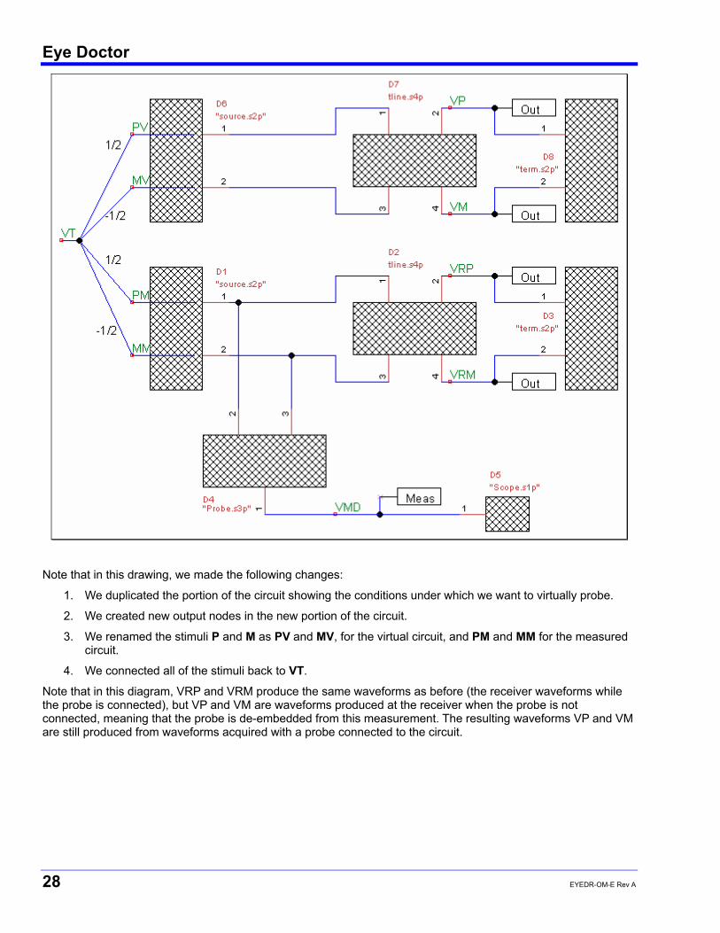
In the previous example, we described a system used to virtually probe the receiver with a probe connected at the transmitter. It is important to note that that example produced output waveforms at the receiver based on waveforms received by the oscilloscope with the probe inserted. In other words, the waveforms produced by such a measurement are waveforms that are only present when the probe is in the circuit. Suppose you want to see waveforms that appear at the receiver when the probe is not connected to the circuit.
To do this, we modify the drawing as follows:
.Device D1 2 File "source.s2p"
.Device D2 4 File "tline.s4p"
.Device D3 2 File "term.s2p"
.Device D4 3 File "Probe.s3p"
.Device D5 1 File "Scope.s1p"
.Node # D1 1 D4 2 D2 1
.Node # D1 2 D4 3 D2 3
.Node VRP D2 2 D3 1
.Output VRP
.Node VRM D2 4 D3 2
.Output VRM
.Node VMD D4 1 D5 1
.Meas VMD
.Stim P D1 1
.Stim M D1 2
.StimDef VT defines P M as 0.5 -0.5
Eye Doctor
28 EYEDR-OM-E Rev A
Note that in this drawing, we made the following changes:
1. We duplicated the portion of the circuit showing the conditions under which we want to virtually probe.
2. We created new output nodes in the new portion of the circuit.
3. We renamed the stimuli P and M as PV and MV, for the virtual circuit, and PM and MM for the measured circuit.
4. We connected all of the stimuli back to VT.
Note that in this diagram, VRP and VRM produce the same waveforms as before (the receiver waveforms while the probe is connected), but VP and VM are waveforms produced at the receiver when the probe is not connected, meaning that the probe is de-embedded from this measurement. The resulting waveforms VP and VM are still produced from waveforms acquired with a probe connected to the circuit.

Eye Doctor Operator’s Manual
EYEDR-OM-E Rev A 29
The system description file for this new system looks like this:
.Device D1 2 File "source.s2p"
.Device D2 4 File "tline.s4p"
.Device D3 2 File "term.s2p"
.Device D4 3 File "Probe.s3p"
.Device D5 1 File "Scope.s1p"
.Device D6 2 File "source.s2p"
.Device D7 4 File "tline.s4p"
.Device D8 2 File "term.s2p"
.Node # D1 1 D4 2 D2 1
.Node # D1 2 D2 3 D4 3
.Node VRP D2 2 D3 1
.Output VRP
.Node VRM D2 4 D3 2
.Output VRM
.Node VMD D4 1 D5 1
.Meas VMD
.Node # D6 1 D7 1
.Node VP D7 2 D8 1
.Output VP
.Node VM D7 4 D8 2
.Output VM
.Node # D7 3 D6 2
.Stim PM D1 1
.Stim MM D1 2
.Stim PV D6 1
.Stim MV D6 2
.StimDef VT defines PM MM PV MV as 0.5 -0.5 0.5 -0.5

Eye Doctor
30 EYEDR-OM-E Rev A
Log Messages
MESSAGE MEANING
(Error) < File Parsing > File Not Found: [Filename] The name of the system description file was not found.
Corrective action is to verify that the name of the file is spelled correctly and that the file exists in the directory specified.
(Informational) < File Parsing > File: [FileName] The name of the system description file is shown as the file being parsed.
(Error) < File Parsing > Null Node Name A node declaration has been found with no node name.
All nodes declared must have a node name followed by a device name and device port number and at least one more device name and device port number.
Corrective action is to examine the file and find the .Node statement that is not followed by a node name, a device name, a device port number and at least one more device name and device port number.
(Error) < File Parsing > Null Device Port Number A node declaration has been found that is not followed by a node name and pairs of device names and device port numbers.
All nodes declared must have a node name followed by a device name and device port number and at least one more device name and device port number.
Corrective action is to examine the file and find the .Node statement that is not followed by a node name, a device name, a device port number and at least one more device name and device port number.
It is important to node that all tokens on a node declaration line are interpreted and device names and port numbers must come in pairs.
(Error) < File Parsing > Nodes must connect at least two device ports
All nodes declared must have a node name followed by a device name and device port number and at least one more device name and device port number.
A node declaration has been found that does not meet this criteria.
Corrective action is to examine the file and find the .Node statement that is not followed by a node name, a device name, a device port number and at least one more device name and device port number.
(Informational) < File Parsing > Devices Counted: [NumDevices]
The number of devices in the system is shown.
(Informational) < File Parsing > Nodes Counted: [NumNodes]
The number of nodes in the system is shown.
(Error) < File Parsing > No Devices There are no devices in the file.
Corrective action is to examine the file and verify that all devices are declared using the .Device statement.

Eye Doctor Operator’s Manual
EYEDR-OM-E Rev A 31
(Error) < File Parsing > Null Device Name A device declaration has been found with no device name.
All devices declared with the .Device statement must have a name supplied (the name is needed to assign nodes to device ports).
Corrective action is to examine the file and ensure that all .Device statements are immediately followed by a device name.
(Error) < File Parsing > Number of Ports: [NumPorts] Invalid
A device has been found with an illegal number of ports.
This usually occurs when the syntax of a .Device declaration is incorrect, as when the device name is not shown or has spaces in it. It can also occur if 0 or negative numbers of ports are declared.
(Error) < File Parsing > Filename must be surrounded by quotes
FileName Given as: [line]
An S-parameter file name has been specified, but the quotes that delimit the filename could not be found.
All S-parameter file names must be enclosed in quotes (to avoid the situation where filenames have spaces embedded).
Corrective action is to enclose all S-parameter filenames in quotes.
(Error) < File Parsing > S-parameter file not read
FileName: [FileName]
The S-parameter file specified was not read.
This occurs when the file is not in a proper Touchstone format. However, there is wide variation in the look of Touchstone files.
Corrective action is to ensure that the file specified actually exists in the directory specified, and that it is a Touchstone format file. If this does not work, try deleting all information from the file except for the line that begins with # (like # MHz S MA R 50.00) and the numbers. If this works, but is inconvenient (for example, you need to edit all of your VNA file outputs), then make sure LeCroy knows about this so we can try to properly accommodate the file format.
Another thing to make sure of is that the amount of S-parameters provided for each frequency matches the number of ports. For example, a file with the extension .s4p defines four-port S-parameters; therefore, for each frequency, there must be 16 S-parameters provided (usually 32 numbers representing the magnitude and phase of the 16 S-parameters).

Eye Doctor
32 EYEDR-OM-E Rev A
(Error) < File Parsing > S-parameter file wrong number of ports
FileName: [FileName]
Wanted: [NumPortsWanted] - Got: [NumPortsGotten]
This means that the number of ports in the S-parameter file does not match the number of ports declared for the device. For example, a 2 port device declaration needs to have an S-parameter file with the extension .s2p.
Corrective action is to ensure that the number of device ports declared is correct and that the extension of the S-parameter file properly matches the desired number of device ports. Note that the S-parameter file format is implied by the extension; so, generally, you cannot correct this problem simply by changing the extension of the S-parameter file.
(Error) < File Parsing > IdealThru must have even number of ports
An idealThru has been declared where the number of ports is not even.
An ideal thru is a device that connects the first half of the ports to the second half of the ports. For example, a four-port ideal thru connects port 1 to port 3 and port 2 to port 4. Therefore, the number of ports must be even.
Corrective action is to confirm that you want an ideal thru for a device, or to correct the number of ports in the device.
(Error) < File Parsing > SingleEndedToMixedModeConverter must have 4 ports
A SingleEndedToMixedModeConverter has been declared where the number of ports is not four.
A SingleEndedToMixedModeConverter has two single-ended ports (ports 1 and 2) and a differential and common-mode port (ports 3 and 4) and, therefore, has exactly four ports.
Corrective action is ensure that this device is declared with four ports.
(Error) < File Parsing > No resistor value provided
A resistor has been declared with no resistance value.
Corrective action is to provide the resistance value.
(Error) < File Parsing > Wrong number of resistor ports
A resistor has been declared with a number of ports other than one or two.
A resistor must be declared with either one or two ports. If declared with one port, the other lead of the resistor is assumed connected to ground.
Corrective action is to ensure that resistors are declared with either one or two ports.
Eye Doctor Operator’s Manual
EYEDR-OM-E Rev A 33
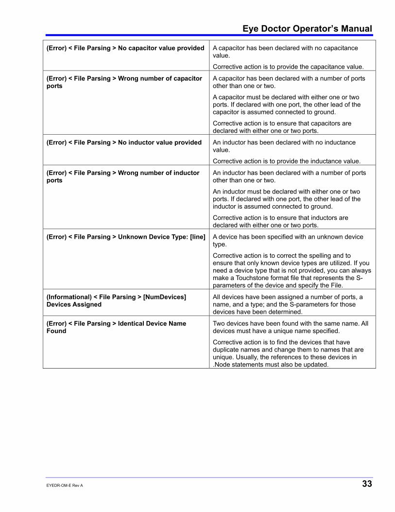
(Error) < File Parsing > No capacitor value provided
A capacitor has been declared with no capacitance value.
Corrective action is to provide the capacitance value.
(Error) < File Parsing > Wrong number of capacitor ports
A capacitor has been declared with a number of ports other than one or two.
A capacitor must be declared with either one or two ports. If declared with one port, the other lead of the capacitor is assumed connected to ground.
Corrective action is to ensure that capacitors are declared with either one or two ports.
(Error) < File Parsing > No inductor value provided
An inductor has been declared with no inductance value.
Corrective action is to provide the inductance value.
(Error) < File Parsing > Wrong number of inductor ports
An inductor has been declared with a number of ports other than one or two.
An inductor must be declared with either one or two ports. If declared with one port, the other lead of the inductor is assumed connected to ground.
Corrective action is to ensure that inductors are declared with either one or two ports.
(Error) < File Parsing > Unknown Device Type: [line] A device has been specified with an unknown device type.
Corrective action is to correct the spelling and to ensure that only known device types are utilized. If you need a device type that is not provided, you can always make a Touchstone format file that represents the S-parameters of the device and specify the File.
(Informational) < File Parsing > [NumDevices] Devices Assigned
All devices have been assigned a number of ports, a name, and a type; and the S-parameters for those devices have been determined.
(Error) < File Parsing > Identical Device Name Found
Two devices have been found with the same name. All devices must have a unique name specified.
Corrective action is to find the devices that have duplicate names and change them to names that are unique. Usually, the references to these devices in .Node statements must also be updated.

Eye Doctor
34 EYEDR-OM-E Rev A
(Error) < File Parsing > Total Number of Device Ports Must be Even
The sum of all device ports in the system is not even.
In the system description, all ports of all devices must be connected to one and only one port of another device. This cannot occur unless the number of device ports is even.
Corrective action is to ensure that all devices have the correct number of ports and that the intent is to connect all of the device ports. If a device port is meant to be unconnected, declare a one-port device of type IdealOpen and connect the port of this device to the intended device port.
(Error) < File Parsing > Number of Ports and Nodes don't match
The total number of device ports is not twice the number of nodes declared.
In the system description, all ports of all devices must be connected to one and only one port of another device. This cannot occur unless the number of device ports is twice the number of nodes declared.
Corrective action is to ensure that all devices have the correct number of ports, that all node declarations have been made connecting all of the device ports, and that the intent is to connect all of the device ports. If a device port is meant to be unconnected, declare a one-port device of type IdealOpen and connect the port of this device to the intended device port.
(Error) < File Parsing > Bad Node Connection
From [ConnectionFromPortName] [ConnectionFromPortNum] To [ConnectionToPortName][ConnectionToPortNum]
A node connection is incorrect. This means either
• one of the device names in the .Node statement could not be found
• one of the port numbers in the .Node statement references a port not found in a device
Corrective action is to verify that the devices named actually exist and that the port numbers specified exist within the devices.
(Informational) < File Parsing > [NumNodes] All of the nodes have successfully been assigned to devices.
(Error) < File Parsing > Device Port Not Connected
Device:[DeviceName] Port:[PortNum]
A port of a device was found that is not connected.
Corrective action is to look at the port number and device name stated and ensure that a .Node statement properly specifies a connection from that device name to that port number. A device port cannot be left unconnected. If the intent is that it is actually left open, declare a one-port ideal open and connect the port of the device to the ideal open.
(Error) < File Parsing > Device Port Connection Incorrect
Device:[DeviceName] Port:[PortNum] - to node labelled [NodeName]?
This is usually an internal error (i.e., should not be encountered if everything else works properly). It means that the system has failed an internal consistency check such that, after the node assignments, the node cannot be found connected to a device.
(Informational) < File Parsing > Device Connections and Nodes Verified
All ports of all devices are correctly assigned to nodes.

Eye Doctor Operator’s Manual
EYEDR-OM-E Rev A 35
(Error) < File Parsing > Stimulus with no name found
A .Stim statement was declared, but no name was stated.
Corrective action is to find the .Stim statement in the file and ensure that the stimulus has a name assigned.
(Error) < File Parsing > Stimulus [StimName] - no device name found
The device named in a .Stim statement could not be found.
Corrective action is to verify the spelling of the device named.
(Error) < File Parsing > Stimulus [StimName] invalid device/port assignment
To Device:[DeviceName] Port:[PortNum]
The device port specified by a .Stim statement does not exist.
Corrective action is to verify that the spelling of the device named is correct and that the port number referenced exists in the device.
(Error) < File Parsing > No Stimuli assigned No .Stim statements were found.
Corrective action is to assign stimuli with the .Stim statement.
(Informational) < File Parsing > [NumStims] Stimuli Assigned
The stimuli defined in the .Stim statements were successfully assigned.
(Informational) < File Parsing > System Defined The system was defined.
This means that a system that allows the calculation of voltages at various nodes with respect to stimuli applied exists. It does not yet mean that voltages at output nodes can be defined in terms of voltages at input nodes.
(Error) < File Parsing > System Not Defined The system could not be defined.
This error should be accompanied by other errors that caused this error. Corrective action is to correct those other errors.
(Error) < File Parsing > .Meas declaration with no node name
A .Meas statement was found without a node name.
All .Meas statements must consist of a node name that specifies a valid node in the system.
Corrective action is to find the .Meas statement with no node name specified and ensure that a valid node name is specified.
(Error) < File Parsing > .Output declaration with no node name
A .Output statement was found without a node name.
All .Output statements must consist of a node name that specifies a valid node in the system.
Corrective action is to find the .Output statement with no node name specified and ensure that a valid node name is specified.
(Error) < File Parsing > Multiple .Stimdef statements found
There can be only one .Stimdef statement in a system description file.
Corrective action is to ensure that there is only one .Stimdef statement.

Eye Doctor
36 EYEDR-OM-E Rev A
(Error) < File Parsing > StimDef with No Actual Stim names
A .Stimdef statement was found with no names of stimuli between the .Stimdef statement and the keyword ‘defines’ in the statement.
Corrective action is to add the stimuli to the .Stimdef statement.
(Error) < File Parsing > Stimdef missing ‘defines’ keyword
A .Stimdef statement was found without the ‘defines’ keyword.
All .Stimdef statements must contain the keywords ‘defines’ and ‘as’.
Corrective action is to verify that the .Stimdef statement is written in the correct form.
(Error) < File Parsing > StimDef with No Stim names A .Stimdef statement was found with no names of stimuli between the word ‘defines’ and the word ‘as’.
(Error) < File Parsing > Stimdef missing ‘as’ keyword
A .Stimdef statement was found without the ‘as’ keyword.
All .Stimdef statements must contain the keywords ‘defines’ and ‘as’.
Corrective action is to verify that the .Stimdef statement is written in the correct form.
(Error) < File Parsing > Stimdef with incorrect numbers defining stimuli relationship
A .Stimdef statement was found without the ‘as’ keyword.
All .Stimdef statements must contain the keywords ‘defines’ and ‘as”. Furthermore, the number of keywords between the .Stimdef and the ‘defines’ keyword defines the number of degrees of freedom. The number of keywords between the ‘defines’ and ‘as’ keyword defines the number of stimuli. The numbers that follow the ‘as’ keyword defines relationships between these degrees of freedom and stimuli. The amount of numbers that define this relationship must be equal to the number of degrees of freedom multiplied by the number of stimuli.
Corrective action is to verify that the .Stimdef statement is written in the correct form.
(Error) < File Parsing > No Measures Found No .Meas statements were found.
Corrective action is to insert .Meas statements stating the nodes where actual waveform acquisitions take place.
(Error) < File Parsing > No Outputs Found No .Output statements were found.
Corrective action is to insert .Output statements stating the nodes where you want to see waveforms output.
(Informational) < File Parsing > Measures Counted: [NumMeas]
Measures were found and assigned.
(Informational) < File Parsing > Outputs Counted: [NumOut]
Outputs were found and assigned.

Eye Doctor Operator’s Manual
EYEDR-OM-E Rev A 37
(Informational) < File Parsing > Degrees of Freedom Specified: [NumDeg]
With Respect to [NumStims]
The number of degrees of freedom in the system has been determined (from a .StimDef statement) based on a number of stimuli.
(Informational) < File Parsing > Measures, Outputs and StimDefs Assigned
The measure nodes, output nodes, and stimuli have been assigned.
(Informational) < System Def > Stimulus and Node Vector Built
A vector of voltage node names and stimuli has been built.
(Informational) < System Def > System Characteristics Matrix Built and Inverted
For each frequency, the system characteristics matrices have been determined from the S-parameters supplied and inverted.
(Informational) < System Def > System Characteristics Matrix and Stimuli Vector Reduced
Once the S-parameter matrices for each frequency are built and inverted, the matrices are reduced in order, based on the number of stimuli. This is a calculation optimization.
(Informational) < System Def > Node Voltage Vector Built
The inverted, reduced systems characteristics matrices are multiplied by the voltage extraction matrix and the node voltage vector. The node voltage vector has been built.
(Informational) < System Def > Voltage Extraction Matrix Built
The inverted, reduced systems characteristics matrices are multiplied by the voltage extraction matrix and the node voltage vector. The voltage extraction matrix has been built. The voltage extraction matrix is one that converts a and b power waves in the system to actual voltages.
(Error) < System Def > Measure Voltage [VoltageName] Not Found
A voltage node declared with a .Meas statement was not found. Corrective action is to verify that the spelling of the node named is correct and that the node exists.
(Error) < System Def > Matrix Not Invertible The number of measure nodes does not match the number of stimuli defined in the .StimDef statement. In order to produce filters, the number of stimuli defined immediately after the .Stimdef statement (before the word ‘defines’) must match identically the number of .Meas nodes. Currently, the system does not handle over-constrained cases (one where the number of measure nodes exceeds the number of stimuli). Corrective action is to add or reduce the number of measure nodes or add or reduce the number of stimuli so that the necessary condition is met.
(Error) < System Def > Output Voltage [VoltageName] Not Found
A voltage node declared with a .Output statement was not found. Corrective action is to verify that the spelling of the node named is correct and that the node exists.
(Informational) < System Def > Writing Responses Writing the frequency responses that will define the filters to disk.
(Informational) < System Def > Response: [ResponseFileName]
Writing a particular frequency response to disk that will define a particular filter.
(Informational) < System Def > Writing Filters Writing the filter impulse responses to disk.

Eye Doctor
38 EYEDR-OM-E Rev A
(Informational) < System Def > Filter: [FilterFileName]
Writing a particular impulse response to disk.
(Informational) < Filters > Reading Filters Reading filters from the disk.
(Informational) < Filters > Output Selection: [OutputName]
Names the output that has been selected.
(Informational) < Filters > Filter: [FilterFileName] Names the filter on the disk that is being read.
S-Parameter Files
Touchstone Format
Touchstone is a file format used for specifying S-parameters. It is a standard that is commonly adopted by vector network analyzers (VNAs), time-domain network analyzers (TDNA) and EDA tools such as microwave simulators. The Virtual Probing component interprets Touchstone files in the following manner:
1. The extension must be in the form “.s[N]p” where [N] corresponds to the number of ports in the device. For example, a two port S-parameter file has an extension “.s2p”.
2. Lines cannot be longer than 2000 characters.
3. Lines beginning with ‘!’ are comment lines. Comments must be at the front of the file. No comments are allowed once the frequencies and S-parameter values start.
4. There should be at least one line that begins with ‘#’. This line is a line that contains tokens that help interpret the S-parameters. Valid tokens are:
a. Hz – frequencies are in Hz.
b. MHz – frequencies are in MHz.
c. GHz – frequencies are in GHz.
d. MA – S-parameters are in magnitude/angle form where the magnitudes are true magnitudes and the angle is in degrees.
e. RI – S-parameters are in real/imaginary form.
f. DB – S-parameters are in magnitude/angle form where the magnitude is in decibels and the angle is in degrees.
5. If the above tokens are not found, the frequencies are assumed to be in MHz, and the S-parameters are assumed to be in magnitude/angle form.
6. The S-parameters for each frequency are assumed to be listed as [frequency] (S11) (S12) …(S1[N]) (S21) (S22) … (S2[N]) … (S[N]1) (S[N]2) … (S[N][N]), where N is the number of ports dictated by the file extension, except for two-port S-parameters which are assumed to be listed as [frequency] (S11) (S21) (S12) (S22) according to the standard.
7. All S-parameters are assumed to be 50 Ohm. In S-parameter files, on the line beginning with ‘#’, usually there is a token pair: R [Z0] where [Z0] is the characteristic impedance. We assume Z0 is 50 and ignore these tokens.
8. All frequencies are assumed to go from the first frequency listed to the last frequency listed with constant frequency spacing.
Other Notes about S-parameter file interpretation and usage.
S-parameters provided to the virtual probe will tend to have various frequency scales, differing in both resolution (frequency spacing) and range (start frequency and end frequency). The virtual probe component will resample all S-parameter sets onto a new frequency scale dictated by the system sample rate (half the sample rate will be the last frequency) and the time length (see Time Length) – where the time length dictates the new frequency resolution. In performing this resampling, it is important to understand that the resolution may be higher or lower than the original resolution and that the frequency range may require extrapolation of points. When the frequency
Eye Doctor Operator’s Manual
EYEDR-OM-E Rev A 39
range is higher than that provided in the S-parameter data (i.e. the S-parameters are not provided to half the system sample rate), then the S-parameter data will be set to zero at these extra required data points. Furthermore, most S-parameter data does not go to DC, because VNAs don’t measure data to DC, and therefore the DC response is also extrapolated by setting the low frequency points equal to the first frequency provided in the S-parameter data.
What this means is that it is helpful to follow some simple rules that will maximize the effectiveness of the virtual probe:
1. Take S-parameter data as low in frequency as the VNA allows to minimize DC extrapolation errors.
2. Take S-parameter data up to one half of the system sample rate. In other words, if you are going to supply waveforms to the virtual probe at 40 GS/s, it is good to provide data up to 20 GHz. Otherwise, if the frequency content of the signal provided to the system is much lower, then it is unnecessary to sample at a high sample rate anyway.
3. Take S-parameter data with sufficient frequency resolution. The resolution that needs to be provided depends on the electrical lengths of the circuit elements involved. In other words, if you have a cable that is 5 ns long, and there are reflections going on in the system, then taking data at maybe one tenth the minimum frequency resolution of 1/5 ns = 200 MHz (like 20 MHz) is a good idea. Said differently, in a more practical manner, if there are lots of bumps and wiggles in the S-parameters that are narrow in frequency, then you will need to measure S-parameter data with an appropriate frequency resolution to capture these bumps and wiggles. Usually the narrowness of the bumps and wiggles becomes smaller when the electrical lengths of circuit elements becomes longer.
Mixed-mode S-parameters
Mixed-mode S-parameters are S-parameters that were devised to help in the analysis of differential systems. In differential systems, they are more meaningful to examine than single-ended S-parameters. There is an equivalence between single-ended and mixed-mode S-parameters and used properly, there is no need (other than examination of the parameters as previously mentioned) to use mixed-mode S-parameters in simulation or in virtual probing. That being said, there are often times when mixed-mode S-parameters are all that is available. For example, many VNAs will output S-parameters as mixed-mode, if so instructed. Furthermore, some systems will measure only portions of the mixed-mode parameters, so some mention is deserved here.
A four port device, such as a differential transmission line is represented as single-ended S-parameters as a four by four matrix. The individual S-parameters are not overly useful for examination unless the two differential lines are not coupled. When the lines are coupled, it is necessary to convert them to mixed-mode S-parameters for examination. This is accomplished through well known formulas and results in another four by four matrix. This matrix can be further thought of as four quadrants of two by two S-parameters.
In single-ended S-parameters, we consider the S-parameters to represent relationships between incident and reflected waves at each of the four ports. In mixed-mode S-parameters, we assume that the two leftmost ports and the two rightmost ports of the single-ended network represent the positive and negative lines of a differential signal. In mixed-mode S-parameters, we think of the two leftmost ports and the two rightmost ports as the differential and common mode components and further think of the mixed-mode S-parameters as presenting relationships between incident and reflected differential and common mode components. Sometimes, a simplification is used and we ignore the common mode ports (assume that they don’t exist), consider only the differential mode, and further assume that no “mode conversion” takes place. In this simplification, we think of the differential line represented as a two port device with two differential mode ports. The two port S-parameters in this case represent the differential-differential mode response of the network.
Before continuing, it must be reiterated that while this assumption can sometimes be useful in the examination of the behavior of the differential line, this oversimplification is seldom necessary when using the virtual probe component and we recommend the use of the single-ended four port S-parameter representation.
If mixed-mode S-parameters are supplied, some very important complications and considerations must be taken into account:
1. The reference impedance for the differential mode S-parameters are assumed to be 100 Ohms (i.e. a perfect differential match is a 100 Ohm differential termination).
2. The reference impedance for the common mode S-parameters are assumed to be 25 Ohms (i.e. a perfect common mode match is a 25 Ohm common mode termination.

Eye Doctor
40 EYEDR-OM-E Rev A
3. You must be very careful to identify the differential and common mode ports – it is less easy to distinguish this in mixed-mode S-parameters than in single-ended S-parameters.
If you are provided with mixed-mode S-parameters in this form, you can directly use them with the virtual probe, provided you utilize single-ended to mixed-mode converters (see
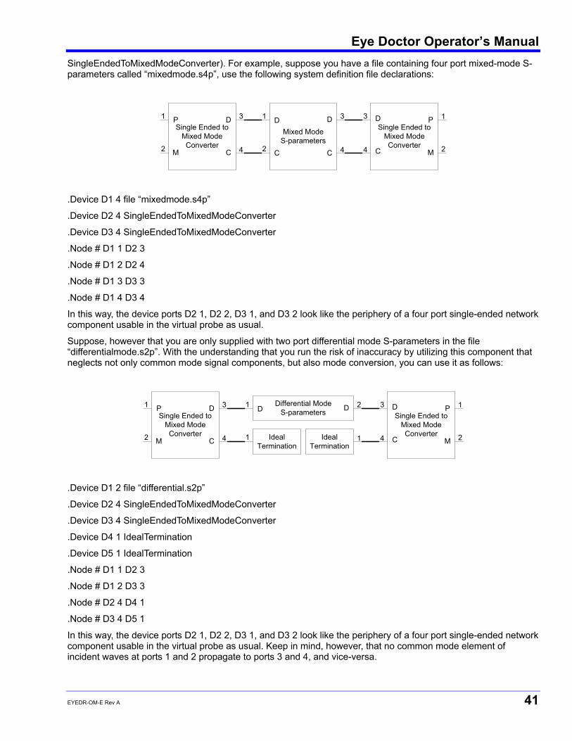
Eye Doctor Operator’s Manual
EYEDR-OM-E Rev A 41
SingleEndedToMixedModeConverter). For example, suppose you have a file containing four port mixed-mode S-parameters called “mixedmode.s4p”, use the following system definition file declarations:
Mixed ModeS-parameters
Single Ended toMixed ModeConverter
Single Ended toMixed ModeConverter
1 D D
C C
D
C
D
C
P
M
P
M
1
2
3
42
3
4
3
4
1
2
.Device D1 4 file “mixedmode.s4p”
.Device D2 4 SingleEndedToMixedModeConverter
.Device D3 4 SingleEndedToMixedModeConverter
.Node # D1 1 D2 3
.Node # D1 2 D2 4
.Node # D1 3 D3 3
.Node # D1 4 D3 4
In this way, the device ports D2 1, D2 2, D3 1, and D3 2 look like the periphery of a four port single-ended network component usable in the virtual probe as usual.
Suppose, however that you are only supplied with two port differential mode S-parameters in the file “differentialmode.s2p”. With the understanding that you run the risk of inaccuracy by utilizing this component that neglects not only common mode signal components, but also mode conversion, you can use it as follows:
IdealTermination
IdealTermination
Differential ModeS-parametersSingle Ended to
Mixed ModeConverter
Single Ended toMixed ModeConverter
1 D DD
C
D
C
P
M
P
M
1
1
2
12
3
4
3
4
1
2
.Device D1 2 file “differential.s2p”
.Device D2 4 SingleEndedToMixedModeConverter
.Device D3 4 SingleEndedToMixedModeConverter
.Device D4 1 IdealTermination
.Device D5 1 IdealTermination
.Node # D1 1 D2 3
.Node # D1 2 D3 3
.Node # D2 4 D4 1
.Node # D3 4 D5 1
In this way, the device ports D2 1, D2 2, D3 1, and D3 2 look like the periphery of a four port single-ended network component usable in the virtual probe as usual. Keep in mind, however, that no common mode element of incident waves at ports 1 and 2 propagate to ports 3 and 4, and vice-versa.

Eye Doctor
42 EYEDR-OM-E Rev A
Mixed-mode S-parameters are an invitation to mistakes in simulation and in virtual probing and certainly the use of two port differential-mode-only views of differential network elements is dangerous. Even when signals only contain differential components (i.e. perfectly balanced transmitters), it is important to note that usually there is some amount of mode conversion at either the transmitter or receiver termination and that common mode signals will usually be present and will usually have some effect on the differential mode signals.
System Descriptions The most important concept to Virtual Probing, and the most abstract, is the system diagram that describes the problem to be solved. This section attempts to provide insight into making the diagram that is later converted to a system description file.
In order to most easily understand how to generate this diagram, it helps to divide the problem into two pieces:
1. The measurement configuration – describes how the waveforms move in the system and get into the oscilloscope.
2. The output configuration – describes desired system output waveforms.
Once both the measurement and output configurations have been drawn, both are tied together through related stimuli. Measurement Configuration
The first concept is listed below:
The system diagram must contain all circuit elements in the measurement configuration, including all devices that drive signals into the circuit, and all oscilloscope channels being utilized for the measurement.
This is the absolute minimum configuration, since it describes how signals are generated in the system and how they get to the oscilloscope inputs. It means that:
• Signals cannot come from sources that are not described by the diagram, otherwise these signals will be incorrectly interpreted. Examples of this are cross-talk and power supply noise.
• The oscilloscope channel (a one-port device describing the oscilloscope’s termination) must be shown in the diagram. Furthermore, the node at the oscilloscope connection must be labeled and called out in the system description file in a .Meas statement.
• All places that a waveform can go and reflect from interfaces must be shown.
Some popular examples are shown. Notes about these configurations follow:

Eye Doctor Operator’s Manual
EYEDR-OM-E Rev A 43
Single-Ended High Impedance Probe Connection at Transmitter
Differential High Impedance Probe Connection at Transmitter
VD
1
2
3
4
D3
1
D4
P
C1
1
2
D2
M
Meas
-0.5
1
2
D1
0.5
1
2
3
D5
Meas
1 2
D2
1 2
D3
C2
C1
1
2
D6
1
D5
P
M
Meas
1
D4
1
2
3
4
D7
1
2
D1

Eye Doctor
44 EYEDR-OM-E Rev A
Single-Ended 50 Ohm Probe Connections at Transmitter
50 Ohm Differential Probe Connection at Transmitter
Single-Ended High Impedance Probe Connection at Receiver
1
2
D6
Meas
M
1 2
D2
1
D4
1 2
D3
1
D5
C2
1
2
D1
1
2
3
4
D7
P
Meas
C1
M
P
1
2
3
D3
-0.5
Meas
0.5 1
VD
1
2
D1
C1
C 1
2
D
1 2
D
P
M
Mea
1
D
Mea
1
D
1 2
D
C

Eye Doctor Operator’s Manual
EYEDR-OM-E Rev A 45
Differential High Impedance Probe Connection at Receiver
-0.5
0.5
Meas
M
P
1
D4
1
2
3
4
D3
1
2
D2
1
2
3
D5
VD
1
2
D1
C1
Single-Ended 50 Ohm Probe Connections at Receiver
1
2
3
4
D6
M
1 2
D2
1 2
D3
1
D4
C11
2
D1
P
Meas
1
D5
Meas
C2
50 Ohm Differential Probe Connection at Receiver
M
P
1
2
3
D3
-0.5
Meas
0.51
2
3
4
D4
1
D2
VD
1
2
D1
C1
Notes:

Eye Doctor
46 EYEDR-OM-E Rev A
1. In all diagrams, transmitters are on the left, backplanes are in the middle represented as four port devices, and terminations are at the right.
2. In all cases, high impedance probes are a “tee” in the line (i.e. join to the node with a dot). Fifty (50) Ohm probes terminate the line.
3. Scope channels are a one port element (termination) with the node between the oscilloscope channel and the probing element labeled and designated as a measure. The labeled node is the voltage developed at the oscilloscope channel port and represents a voltage seen by the oscilloscope.
4. Stimuli emanate from both device ports of the transmitter and are designated P and M (for the plus and minus signals, respectively).
5. In the case of differential measurements, there are two stimuli, but only a single measurement node. Therefore, to a single degree of freedom is shown as VD with the stimuli P and M shown related to VD assuming perfect balance. (i.e. P is ½ of VD and M is -½ of VD). This would be called out in a .Stimdef statement (e.g. .Stimdef VD defines P M as 0.5 -0.5).
6. All elements shown in these measurement configurations are important and cannot be ignored. They are all part of the circuit in the measurement.
Output Configuration
The output configuration is a diagram showing the transmitter in a configuration containing nodes that are defined as outputs of the system. When the output configuration and nodes are found in the measurement configuration, then the process is straightforward. In this case, label nodes in the measurement configuration as outputs. In this situation, we can say that the waveforms of interest are those within the circuit with the measurement hardware connected. In other words, the Virtual Probe component will show waveforms that are present in the circuit while the probes are connected.
There are many ways that the output configuration can be different from the measurement configuration. Some common situations are:
1. The output configuration is the same as the measurement configuration, with the only difference being that the probes are not connected. This will generally only be the case for high-impedance probes. In this case, waveforms produced by the virtual probe are waveforms that would be present if the probes weren’t present. This is called probe de-embedding.
2. The output configuration consists of completely different hardware. This can include different transmitter input return loss characteristics, different backplanes, and different terminations. This is called emulation. In emulation configurations, different hardware characteristics can be tried out by simply modifying software characteristics. Often, the characteristics in this configuration are produced through system simulators. In this manner, hardware can be tried without ever even producing it physically.
3. The nodes declared as outputs are at different locations than where the probes are connected. In this way the Virtual Probe component produces waveforms at locations other than the probing point. Sometimes these probing points are inaccessible.
Output Configuration Matches Measurement Configuration
When the desired system waveforms are found in the measurement configuration all that is required is to label the output nodes in the measurement configuration diagram. An example is:

Eye Doctor Operator’s Manual
EYEDR-OM-E Rev A 47
C1
1
2
D1
1 2
D2
1 2
D3
1
D4
1
D5
1
2
D
Meas
Meas
C2
1
2
3
4
D7
P
M
Out
Out
RXM_PR
RXP_PR
C1
1
2
D1
1 2
D2
1 2
D3
1
D4
1
D5
1
2
D
Meas
Meas
C2
1
2
3
4
D7
P
M
Out
Out
RXM_PR
RXP_PR
This is the measurement configuration above (see Single-Ended High Impedance Probe Connection at Receiver). The output nodes RXP_PR and RXM_PR have been added. In this situation, the virtual probe component would produce waveforms at the receiver that are present while the probe is connected. This situation is useful for seeing accurate waveforms at the receiver with any non-ideal probe characteristics affecting the measurement.

Eye Doctor
48 EYEDR-OM-E Rev A
Another example is:
C1
1
2
D1
1
2
D
P
M
1
2
3
4
D3
1
D4
Meas
1
2
3
D5
VD
0.5
-0.5
Out
Out
RXP_PR
RXM_PR
This is the measurement configuration above (see Differential High Impedance Probe Connection at Transmitter) The output nodes RXP_PR and RXM_PR have been added. In this situation, the virtual probe component would produce waveforms at the receiver that are present while the probe is connected at the transmitter. This situation is useful for seeing accurate waveforms at the receiver with any non-ideal probe characteristics affecting the measurement.
Output Configurations Without Probe Connections
In the previous section, we showed output configurations that match the measurement configuration. The output nodes in the measurement configuration show waveforms affected by the probes. Often, it is desirable to see waveforms that would be present without the probes connected. This is accomplished by simply redrawing the measurement configuration, but without the probes connected. The only complexity is that the stimuli must be tied somehow to a number of degrees of freedom that match the number of measurement nodes in the system. An example shows how this is accomplished:

Eye Doctor Operator’s Manual
EYEDR-OM-E Rev A 49
C1
1
2
D1
1 2
D2
1 2
D3
1
D4
1
D5
1
2
D
Meas
Meas
C2
1
2
3
4
D7
PM
MM
Out
Out
RXM_PR
RXP_PR
RXP1
2
D8
1
2
D9
1
2
3
4
D10
PO
MO
Out
Out
RXM
P
M
This is the configuration from the last section, where an output configuration has been added to the circuit. The output configuration is a duplicate of the measurement configuration where the probes are not present. New output nodes RXP and RXM have been added, in addition to RXP_PR and RXM_PR. While RXP_PR shows waveforms present at the receiver with the probe connected, RXP shows waveforms that would be present if the probes were not connected. This is useful for two key reasons:
1. RXP and RXM show what the system performance would be without the probes interfering. In other words, within certain constraints, RXP and RXM will show the same waveform regardless of the characteristics of the probes D2 and D3 and oscilloscope channel return loss D4 and D5. This is useful for compliance testing where the probe is de-embedded from the measurement.
2. RXP and RXM can be compared to RXP_PR and RXM_MR to see how the probe is affecting the waveforms at the receiver during the measurement. This is important because it is very difficult usually to understand the affect that probes have on the measurement, even when provided good measurement data of the probe characteristics. Using Virtual Probing, it becomes possible to see this.
Note that the stimuli have been named PO, MO, PM and MM and have been associated directly with two degrees of freedom, P and M to match the number of measurement nodes. In the system description file, after the stimuli have been defined, a .Stimdef statement would tie these together (e.g. .Stimdef P M defines PO MO PM MM as 1 0 0 1 1 0 0 1). This because PO is 1 times P plus 0 times M, MO is 0 times P plus 1 times M, PM is 1 times P plus 0 times M, and MM is 0 times P plus 1 times M.

Eye Doctor
50 EYEDR-OM-E Rev A
Here’s another example:
C1
1
2
D1
1
2
D
PM
MM
1
2
3
4
D3
1
D4
Meas
1
2
3
D5
0.5
-0.5
Out
Out
RXP_PR
RXM_PR
RXP1
2
D6
PO
MO
1
2
D7
1
2
3
4
D8
VD
0.5
-0.5
Out
Out
RXM
This configuration is the same as the last example except with a differential probe probing at the transmitter. New output nodes RXP and RXM have been added, in addition to RXP_PR and RXM_PR. While RXP_PR shows waveforms present at the receiver with the probe connected, RXP shows waveforms that would be present if the probes were not connected. Note that in this case the stimuli PO, MO, PM, MM are related to the single degree of freedom VD as PO and PM are ½ of VD and MO and MM are -½ of VD, therefore the .Stimdef would look like:
.Stimdef VD defines PO MO PM MM as 0.5 -0.5 0.5 -0.5

Eye Doctor Operator’s Manual
EYEDR-OM-E Rev A 51
Here is an example of a differing output configuration with completely different hardware:
1 2
D1
PO
MO
1
2
D
1 2
D2
1
D3
Out
C2MM
1
2
D5
1
2
D6
Out
RXP
RXM
P
M
Meas
Meas
C1PM
1
D4
1
2
3
4
D8
In this configuration, we see that the measurement configuration is one previously shown (see Single-Ended 50 Ohm Probe Connections at Transmitter) where the transmitter is driven directly into oscilloscope channel inputs. The output configuration consists of the same transmitter, but includes a backplane channel and termination. The output nodes RXP and RXM show what the receiver waveform would look like if this transmitter drove the given backplane into the given termination. In this manner, complete backplane emulation is accomplished, but with real transmitter waveforms. This configuration is useful for testing a transmitter in various channel and termination conditions.

Eye Doctor
52 EYEDR-OM-E Rev A
Equalizer Emulation The equalizer emulation feature of Eye Doctor allows you to emulate ideal equalizers.
The Ideal Equalizer Emulation feature enables the emulation of various equalizer configurations, including:
• linear transversal, tapped delay line, linear feed-forward equalizers.
• clock recovery.
• decision feedback equalization.
The equalizer emulation feature allows you to see the recovered data, clock, and equalized waveform. The equalizers can be specified by tap delay, number of taps, and tap coefficients or they can be automatically trained to optimize settings utilizing blind adaptation.
Eye Doctor Equalization Option The Eye Doctor Equalization option might already be loaded on your oscilloscope. Go to Help – About to show the dialog that contains the list of software options. If the list includes the option code EYEDR_EQ, then your oscilloscope has already been outfitted with the Eye Doctor Equalization option. If not, then installation of the option is accomplished and verified through the Utilities menu. The option requires a unique option key.
In order to obtain the option key for the EYEDR_EQ option, you must provide the oscilloscope ID and the Serial # of the oscilloscope to LeCroy. LeCroy will then provide an option key consisting of 16 hexadecimal digits for entry. Correct installation of the key is indicated by the presence of the EYEDR_EQ option under “Installed Option Keys.”
In addition to the option key, your oscilloscope must have firmware version 5.0.4 or higher. Your current firmware version can be found on the Status tab of the Utilities Setup dialog.
The EYEDR_EW option enables the equalizer emulation features, along with the processing web editor. The processing web editor allows editing of processing configurations through a unique graphical user interface.
Configuration of Equalizer Emulation in the Processing Web The processing web editor is accessed through the Math Setup dialog.

Eye Doctor Operator’s Manual
EYEDR-OM-E Rev A 53
The Math main dialog indicates how the math functions are defined, and provides tabs for each of the definable math functions. Selecting any math function tab allows you to configure a math function.
Along the left-hand side of each math setup dialog there are four options for math function configuration. These are single, dual, graph, and web edit. Web edit is only available with the web editing option (enabled by EYEDR). When web edit is selected, the processing web can be accessed through the Show Processing Web button.
When the processing web opens, you will find all possible waveform sources on the left and all possible waveform outputs on the right (in this case, F1, F2, F3, and F4 are defined as processing web edit waveforms, so these pins are seen on the right).

Eye Doctor
54 EYEDR-OM-E Rev A
To access the Eye Doctor components, select the Add Math button. This displays a dialog containing all math functions available on your oscilloscope. Select the Eye Doctor category to display all of the Eye Doctor processors.
Select EqRcv for the Equalizer Emulation component. The Equalizer Emulation component appears in the processing web. It is a one-input, four-output processor. A dialog is present in the lower right-hand corner that allows access to the internal configuration dialog.

Eye Doctor Operator’s Manual
EYEDR-OM-E Rev A 55
Here the equalized receiver component is shown (along with the virtual probing component previously explained). The goal will be to equalize the waveform at the receiver provided by the virtual probing component.
The input pin to the equalizer receiver component is an analog serial data waveform: ideally, the waveform that appears at the receiver in a system.
The four output pins are:
• Out – the equalized waveform that appears at the input to the slicer in the emulated receiver.
• Data – an ideal data waveform representing the waveform at the output of the slicer in the emulated receiver.
• Clock – an ideal clock waveform representing the clock recovered by the receiver.
• Error – The difference between the waveform at the input to the slicer and the data waveform at the output of the slicer (Out – Data). This signal is used to determine a noise signal with smaller noise signals representing better equalization. This signal can be used with external, user defined equalizer optimization algorithms.

Eye Doctor
56 EYEDR-OM-E Rev A
The equalized receiver is a component actually made up of several internal processors. These processors are all available for use independently within the processing web and include:
• an equalizer optimizer component – determines optimum FFE and DFE coefficients from the input waveform.
• a tapped delay line equalizer – provides linear, feed-forward equalization.
• Time Interval Error component – acts as a PLL that extracts the clock from the tapped delay line equalizer component output.
• a decision feedback equalizer/receiver component – provides decision feedback equalization and serves to determine the decoded data and extracted clock.
• track components that convert the decision feedback, data, and clock times and levels into waveforms.
• a difference component that subtracts the decision feedback from the tapped delay line equalizer output to form the equalized waveform at the slicer input.
• float waveform reframer – frames the outputs appropriately.
It is normally not necessary to build the equalized receiver component from the individual components in the processing web.
Returning to the equalized receiver component, once the component is placed in the processing web, press the Settings button to access the pop-up dialog that sets the configuration. There are three tabs on the dialog:
• Basic – the dialog where you configure the basic characteristics of the serial data waveform, such as bit rate, thresholds, and ideal levels; and where you configure the parameters for the automatic equalizer optimization.
• FFE – the dialog where you configure the linear, feed-forward, tapped delay line equalizer.
• DFE – the dialog where you configure the decision feedback equalizer and slicer.

Eye Doctor Operator’s Manual
EYEDR-OM-E Rev A 57
Basic Equalized Receiver Configuration
The basic equalized receiver configuration dialog provides the capability to:
• configure the basic attributes of the serial data signal.
• configure the equalizer optimization.
The basic attributes of the signal include the Bit Rate, the Threshold that determines the decoding of the bits, and the ideal -1 (0) and +1 (1) levels of the bits. The ideal levels are considered the optimum voltages that the serial data waveform should occupy at the time the bit determination is made by the slicer.
The equalizer optimization settings determine how the equalizers are automatically optimized. Since the equalizer is optimized without utilizing the internal clock recovery component, the framing granularity is used to determine how many gradations are necessary in determining the proper phase of the recovered clock for optimization; it is advisable to leave this number unchanged.
The number of Training Bits is the number of unit intervals to use from the input waveform for equalizer optimization. The number is restricted to a range to avoid overly large or small numbers of waveform points to be used for optimization.
The time and memory required for the calculation will depend on the number of training bits:
• 500≈Bits : 5 seconds = low memory.
• 2000≈Bits : 30 seconds = moderate memory.
• 5000≈Bits : 2 minutes = large amounts of memory.
Note: For large values of training bits (i.e., commensurate large numbers of waveform points used for optimization), the oscilloscope may take an inordinate amount of time to do the calculation, and use up all available memory. Currently, there is no protection from this situation and you must carefully consider the number of training bits used for training. If in doubt, leave the value of Min and Max points at the default values.
During training, the system will not train if the number of input waveform points is less than the Min Training Points. Otherwise, it will use the minimum of the number of waveform points available and the Max Training Points specified.
Weights controls the optimization objective – in some cases you want to optimize edge placement and in other cases you want to optimize the voltage level at the center of the UI where the decision is made. In some cases you want some blend of weighting. Edge Weight and Center Weight allow you to choose this weighting. Internally, the weights are normalized to be value specified divided by the sum of the two weights, so weighting each as 1.0 (the maximum weight) is the same as weighting each as 0.5 (the normalized value).

Eye Doctor
58 EYEDR-OM-E Rev A
The Linear Tapped Delay Line Equalizer optimization is specified by selecting the number of desired taps, from 0 to 20. A specification of 0 means that the FFE is not used. A specification of one tap means that the FFE provides only gain/attenuation and is the minimum setting. Otherwise, the pre-cursor taps determine the cursor location within the taps specified. As an example, if four taps are specified and one pre-cursor tap is specified, the resulting filter will have four coefficients, with coefficient 1 (the second coefficient) representing the cursor.
The Decision Feedback Equalizer optimization is specified by selecting the number of taps from 0 to 20. A specification of zero means that the DFE is not used. The first tap (tap 0) is taken directly from the slicer output. Subsequent taps are taken from delayed versions of the slicer output.
It is important to note that none of the equalizer optimization settings have any effect on the processing of waveforms (only on the filter optimizations) and, as such, has no effect until filter training commences.
To train the equalizer on an input waveform, make all of the aforementioned configurations and press the Train button in the dialog.
To clear the equalizer so that it performs no actual equalization, press the Clear button in the dialog.

Eye Doctor Operator’s Manual
EYEDR-OM-E Rev A 59
Note: Equalizer training will not take place unless the following criteria are met:
1) a waveform is present at the input pin of the component.
2) a consumer of an output pin of the component is active.
To ensure this is the case, view the output waveforms from the equalized receiver prior to equalizer training.
The result of the equalizer optimization is to update the configuration of the FFE and DFE in the other setup dialogs. Specifically:
• The number of FFE delay taps is set to the number of taps specified.
• FFE Tap Delay is set according to the bit rate and the number of samples per UI.
• FFE Tap Weights are set optimally.
• DFE Delay Taps is set according to the number of taps specified.
• DFE Tap Weights are set optimally. Feed Forward Equalizer (FFE) Configuration
The FFE configuration sets the configuration of the linear tapped delay line equalizer. Usually, these values are set as a result of equalizer optimization. You can view the results in this dialog, or set them manually or by using your own optimization algorithms.
The values in this dialog page directly determine how waveforms are processed, and changing these values will have immediate effects on waveforms being displayed.
The configuration of the FFE includes:
• The number of FFE Delay Taps.
• The number of pre-cursor Taps.
• Tap Delay (usually 1 or ½ the unit interval).
• Tap Weights – the filter coefficients.
The filter output is always taken from the cursor tap (The tap with a tap number corresponding to the number of pre-cursor taps).

Eye Doctor
60 EYEDR-OM-E Rev A
Decision Feedback Equalizer (DFE) Configuration
The DFE configuration sets the configuration of the decision feedback equalizer. Usually, these values are set as a result of equalizer optimization. You can view the results in this dialog, or set them manually or by using your own optimization algorithms.
The values in this dialog page directly determine how waveforms are processed, and changing these values will have immediate effects on waveforms being displayed.
The configuration of the DFE includes:
• the number of DFE Delay Taps.
• the Tap Weights – the filter coefficients.
During operation, the DFE performs the following operations:
1. On falling clock edges, the waveform at the input to the slicer is sliced, meaning that it is compared to the threshold value. If it is above the threshold value, the voltage is set to the ideal +1 voltage previously described. If is below the threshold, it is set to the ideal -1 voltage previously described.
2. The sliced voltage is presented to a line of delay taps (one tap per UI).
3. On the rising edge of the clock, the DFE filter (of given length and coefficients) is applied to the sliced voltage values in, and at the front of, the delay taps.
4. The DFE filter output is fed to a differential element that subtracts the DFE filter output from the input to the DFE component, and presents it to the slicer.
5. Steps 1-4 are repeated. Note: The DFE filter is a filter applied to voltages, not ones and zeros.
Note: Normally, an actual DFE tries to apply the feedback immediately after the decision has been made (i.e., as soon as the waveform is sliced) to give it time to affect subsequent decisions. This DFE is ideal in the sense that the feedback signal can be applied instantaneously. However, the feedback is held off until the rising clock edge so that the resulting eye can be realistically analyzed for jitter measurement reasons.
The DFE and slicer configuration has two additional elements:
• Clock Adjust.
• Erasure DFE.

Eye Doctor Operator’s Manual
EYEDR-OM-E Rev A 61
Since there is often an optimal setting of the clock relative to the data entering the slicer, the clock placement is adjustable. The clock adjustment is such that if positive numbers are entered, the clock moves backward relative to the data and the data is sampled earlier. Note: The equalizer optimization does not utilize the same clock extraction as the PLL. Therefore it is sometimes necessary to adjust the clock following equalizer training to obtain the same, optimal result.
DFEs are prone to burst errors (i.e., errors that, once created, run for a long time). The DFE’s propensity to create burst errors is based on the fact that the effectiveness of the DFE to aid in the accurate decoding of bits depends on its ability to accurately decode bits — a circular situation. Depending on the strength of DFE applied, a single bit error may lead to a long run of errors. To improve the situation, erasure DFE is used. Erasure DFE effectively sets a band around the threshold value. When the signal falls inside this band at the time of slicing, this indicates an uncertainty in the bit decoding, and the receiver, although obliged to decode the bit, can decide not to apply this bit to the decision feedback, since the decoding was not certain enough. In operation, if erasure DFE is utilized and the signal is within the voltage delta about the threshold specified, a voltage value that is the average of the ideal +1 and -1 values is applied to the DFE delay taps, thus causing the bit to have no effect on decision feedback. Note: When erasure DFE is used, erasures appear in the decoded-data waveform as data bits that end up half way in between the ideal voltage levels for the bits.
Connection of the Equalized Receiver
A connectivity diagram of the equalized receiver component is shown above. This connection allows the unequalized waveform to arrive at F1, the equalized waveform to arrive at F2, and the data and clock waveform to be shown on F3 and F4, respectively. An upsampler was placed in-line to create better looking waveforms.

Eye Doctor
62 EYEDR-OM-E Rev A
Equalized Receiver Example The remainder of the equalized receiver information is provided by using an example.
Consider the situation in which the waveform probed at the receiver is a 7.75 Gb/s NRZ 127 bit pattern. Consider that the ideal levels of the waveform are 200 mV and -200 mV with the threshold being at 0. We want to see the unequalized waveform on F1, the equalized waveform at F2, and the data and clock waveforms on F3 and F4.
This leads to settings as shown in the basic configuration of the equalized receiver:
The math waveforms are turned on using the math setup menu:
You will see the unequalized waveform at the receiver on the top, followed by the same unequalized waveform (we have not yet optimized the equalizer), followed by the data waveform, followed by the clock waveform.
Note especially that the unequalized waveform has a gap at left and right due to filtering considerations in generating the waveform at the receiver; the waveforms output from the equalizer have these same gaps. Furthermore, the data and clock waveforms exhibit startup issues; here the clock takes almost 40 ns to get going. Usually, you do not want to see the startup situation. Since the oscilloscope does not receive a continuous waveform on each waveform acquisition, it will need to start things up. To avoid seeing this lag, zoom in sufficiently on the waveform. Note: To avoid seeing startup issues with the equalizer, do not adjust the timebase setting of the acquisition system; this will not accomplish the objective. Use the zoom feature instead.

Eye Doctor Operator’s Manual
EYEDR-OM-E Rev A 63
Since all of these waveforms need to be zoomed together, use the MultiZoom capability to lock the zooms of the traces.
In the figure above, Zoom Setup… is selected from the Math drop-down menu. Then the MultiZoom tab is selected, and Multi-Zoom is turned On. All of the desired math traces for the Multi-Zoom are selected. The Auto-Scroll controls to the right are used to scroll through the zoomed traces.

Eye Doctor
64 EYEDR-OM-E Rev A
At this point, it is useful to superimpose the unequalized, equalized, and data waveforms on top of each other. This is done by selecting Display in the menu bar, then Dual grid. Select the math trace, then touch Next Grid:
At this point, all waveforms appear in the top grid except for the clock waveform, which appears at the bottom. By looking at the decoded-data waveform, you can see that there are many bit errors, and the data is clearly not decoded well due to the distortion of the waveform.

Eye Doctor Operator’s Manual
EYEDR-OM-E Rev A 65
We configure the equalizer optimization for equal weighting of the edge and center, three FFE taps (center tapped) with two samples per UI, and two DFE taps:
Pressing the Train button causes the equalizer to be optimized with these settings, and you will see changes in the displayed waveforms:
We see that the equalized waveform performs much better and the decoded bits are correct.

Eye Doctor
66 EYEDR-OM-E Rev A
The FFE and DFE tabs show the equalizer settings resulting from the optimization:
At this point you can experiment with your own equalizer optimization settings, or select your own equalizer tap and coefficient values.
More importantly, you can analyze the jitter with the normal SDA functionality. To do this, you should zoom out on the waveforms (to get at least a few patterns on the screen).

Eye Doctor Operator’s Manual
EYEDR-OM-E Rev A 67
When using Eye Doctor in conjunction with the SDA analysis software, and especially if the DFE is used, ensure that you uncheck the Recover clock checkbox, and use the clock provided at the equalized receiver component output.
When using the recovered clock from the equalized receiver component, it helps to use an upsampler to improve the time resolution of the clock edges. This is done by selecting Add Math, then Interpolate from the pop-up menu.
Alternately, it is advantageous to place an upsampler in front of the equalizer component (in which case, it is usually not necessary to upsample the clock waveform).
§ § §